������������������� �� ������������������������������������������������������

10.5121/ijsea.2010.1202 14

Optimized Test Sequence Generation from Usage Models using Ant Colony

Optimization

Praveen Ranjan Srivastava1, Nitin Jose2, Saudagar Barade3, Debopriyo Ghosh4

1,2,3,4 Departments of Computer Science and Information Systems, BITS-Pilani

Pilani - 333031, Rajasthan, India 1, 2, 3, 4{praveenrsrivastava, jose.nitin, ssbarde, debopriyoghosh} @gmail.com

ABSTRACT Software Testing is the process of testing the software in order to ensure that it is free of errors and produces the desired outputs in any given situation. Model based testing is an approach in which software is viewed as a set of states. A usage model describes software on the basis of its statistical usage data. One of the major problems faced in such an approach is the generation of optimal sets of test sequences. The model discussed in this paper is a Markov chain based usage model. The analytical operations and results associated with Markov chains make them an appropriate choice for checking the feasibility of test sequences while they are being generated. The statistical data about the estimated usage has been used to build a stochastic model of the software under test. This paper proposes a technique to generate optimized test sequences from a markov chain based usage model. The proposed technique uses ant colony optimization as its basis and also incorporates factors like cost and criticality of various states in the model. It further takes into consideration the average number of visits to any state and the trade-off between cost considerations and optimality of the test coverage.

KEYWORDS Model Based Testing, Software Testing, Markov Chain, Ant Colony Optimization, usage model, test sequence generation, stochastic process

1. INTRODUCTION Software Engineering [1] is the use of concrete engineering principles to create cost-efficient and reliable softwares. A trivial definition of Software testing [1], [2] is that it is the process of checking the software for any errors or bugs. A more detailed look into the software testing process reveals that it uses a large number of techniques to ensure that the software accords with the user requirements and that it is reliable. At a very primary level, software testing can be divided into two broad categories namely whitebox testing [1] and blackbox testing [1]. The whitebox approach involves the internal program structure of the software whereas the black box approach [3], [4] views the software as a function which accept some input and produces some desired output. The testing process checks whether any given input yields the expected output. “Model based testing (MBT) is the automation of the design of black-box tests” [2]. It essentially follows the principle of viewing the software as a set of states (S0, S1, … , Sn) where each Si in (S0, S1, … , Sn) can be thought of as the state of the software after a series of inputs to the software (say i0, i1, … , in ) . Model based testing is basically a manifestation of the black box testing [1]. The actual outputs are compared with the expected outputs and a report is generated. To further enhance the capabilities of model based testing we use statistical data. Statistical model based testing uses statistical data of one or more of the software’s attributes to model the software under test (SUT). Markov chains [5] are an appropriate choice for statistical

������������������� �� ������������������������������������������������������

15

model based testing as their inherent properties facilitate the checking of the feasibility of test sequences as they are being generated. In mathematics, a Markov chain [5] is a random process where all information about the future state can be deduced from the current state i.e. there is no need to keep information about the past. The Markov chain based statistical MBT uses markov chains to model the SUT. It was introduced by Whittaker, Thomason, Walton, Poore and others (refer [6], [7], [8], [9]) and is a very effective way of modeling a software under test. It is based on the distribution of operational frequencies among the states in the model. Every state of the SUT will not be operated or used at the same frequency and hence this fact can be exploited in building a model that is based on this operational frequency. This will give an effective way to identify paths in the model which are of greater importance and hence in greater need of being tested. The model which will be used in this paper is a usage model [10]. The usage model consists of a set of states with transitions between them. The transitions are weighed by the probability of the transition. Now, it would be a cost intensive and time consuming task to test all the possible combinations of states and transitions (exhaustive testing [1]). It is necessary to identify an optimal set of walks in the model (called test sequences) which will be sufficient to test a SUT successfully, without resorting to exhaustive testing. SECTION 2, 3, 4, 5 will have an elaborate discussion about the modeling technique discussed above and further discuss a technique for generating optimal test sequences from such a model. A major constraint in any software development process is cost. Cost can be described as a function of the effort which needs be invested in any process. It is commonly expressed in terms of person-months [1]. In order to generate an optimized set of test sequences it is essential to include cost-efficiency. Namely, all states and transitions should be covered in the minimum cost possible. In the technique proposed it has been ensured that cost considerations are being taken into account. The cost_limit factor explained in SECTION 5 addresses this issue. Ant colony optimization (ACO) fits quite well into the problem solution as it in itself is a stochastic process. Markov chain based usage models have been used for the application of ACO because it is desirable to bring some order into the stochastic process of ACO. The ants will make a more precise decision if the operational frequency also acts as a guide during the walk, and hence we arrive to a more effective result; converging quickly to them. Doerner and Gutjahr [11] have used ACO for test sequence generation in markov chain based usage models, but the proposed technique discussed in this paper, also takes into consideration the criticality of the states and the need to cover the most critical states and their attached transitions, even if cost limitations are very strict. The average number of visits to each state [12] have been further incorporated. It is yet another important measure of usage of the software under test. Hence, the proposed technique generates optimal test sequences, so that exhaustive testing can be avoided while incurring minimum cost overheads. A layout of the following sections is as follows. Section 2 discusses the basics of markov chain based usage model. Section 3 discusses the concept of average number of visits to any state. Section 4 discusses Ant Colony Optimization. Section 5 discusses a new stochastic technique for generating test sequence generation from markov usage models. Section 6 analyses the results obtained. Section 7 compares the results obtained from the discussed technique to the results of some existing and previously proposed techniques. Section 8 discusses the conclusions from our work.

2. MARKOV CHAIN BASED USAGE MODEL Markov chain usage based models are built and used to model an SUT on the basis of its expected usage once it has been released. It can be a powerful tool to analyze the usage of the software and further generate test sequences and test cases, having a clear idea of the stopping criteria [10], [6], [13], [14]. They can be essentially viewed as directed graphs with the weights attached to the edges (or transitions). The weights are the probability of the corresponding transition, which in this case, is the operational frequency or the probability of the transition occurring. Consider a graph described by a tuple (V,E). Here V and E are the set vertices (or states as in this case) and the set of edges (or transitions as in this case), respectively. The

������������������� �� ������������������������������������������������������

16

weight attached to the edges is the probability pij = p(j / i) where i, j � ∈ V and {i,j} ∈ E. Before such a model is built, certain assumptions have been made. Namely, (1) all states of the SUT are known, (2) all the transitions are known, (3) the probability of the occurrence of each of the transition is known. Talking about a state in the model doesn’t necessarily mean that it refers to different components or modules of the software. State in a more generic way refers to a state that one might encounter, once a series of inputs have been fed to the system. Each state will have a set of inputs that lead to it from preceding states and a set of inputs that lead out to other states. This is analogous to a finite state machine [15] in the automata theory. Now another question that has been encountered is regarding the methods of estimating the transitional probabilities. A software in use can be an easy subject as the usage patterns are already known. But for a software that has not been released estimating the usage patterns becomes a tricky task. The operational frequency of any given SUT can be estimated by interacting with the target users. Another more reliable method could be estimating the usage by looking at previous versions or prototypes [6] of the software, if any. If no such preceding versions are available for study then similar softwares or systems which have already been released can be used to study usage patterns. Once all this data has been collected one can move ahead to building a model. An example has been given below in Figure 1.

Figure1. A sample model of a web based database interaction service

Figure 1 shows an example a usage model. If we visualize this as a directed graph G (V,E), with the set of vertices V = {Entry, Login, Generate_Report, Change_Profile, Exit} and the set of edges{ { Entry, Login }, { Login, Generate_Report}, { Login, Change_Profile }, { Login, Exit }, { Generate_Report, Exit },{ Change_Profile, Exit } }. The transitional probabilities have been assigned to all the edges in the Figure 1. At any given node, the sum of all the probabilities attached to the outgoing transitions is 1. This is quite evident by the fact that probability of transition from any given state, which has only one outgoing transition, is 1 (except for Exit state which acts like a sink). Furthermore, it must be noted that the probability attached to any edge i,j where {i,j}� ∈ E and i, j ∈ V is essentially the conditional probability pij = p(j/i) i.e. the probability of j occurring given that current state is i.

2.1. Criticality of the state Testing is the most cost intensive phases of software development. It has been estimated that testing consumes 40 to 50 percent of the development effort [1]. Hence it is obvious that cost

������������������� �� ������������������������������������������������������

17

consideration will come into play. Although, work has been done on maintaining a trade-off between cost considerations and coverage [11], it is necessary to ensure that even if full coverage may not be possible at a given strict cost limitation; it must be ensured that all the critical states must be covered and consequently their attached transitions be covered. Hence, one more aspect which needs to be taken into consideration is the criticality of any given state. Now estimation of the criticality of any state and measuring it by a quantifiable metric is a task which must involve both the user and the developer. They will have a differing perspective about the importance of any part of the software. One more important source could perhaps be the project manager. So in order to maintain a fair view about the criticality, we are assuming that these values have been taken for each state from the project manager, developer and user. These values are on a scale of 1 to 100 and each value is the average of all three values i.e. from the project manager, developer and the user. In the following sections criticality of any given state i will be denoted by CRi.

3. AVERAGE NUMBER OF VISITS The average number of visits [12] to any state is yet another measure of operational frequency. It is a measure of how many times a state will be visited. Calculation of this metric is based on the values of average number of visits of the preceding states and the transitional probability between the current state and its preceding states. Similar work has been in done on average visit length at any given state by Prowell [10], [13], [16]. Once again the model is visualized as a graph G (V,E). For any given node i ∈ V the value of average visits is given by AVi. The following formula gives this value.

AVi = Σ AVk x pik (1)

For all k = 0 to n. where n is the total number of nodes. And i,k ∈ V. pik is the transitional probability of {i,k}∈ E. Hence this value can be calculated using the above formula. It must be noted that when i = k this formula becomes recursive. AV1 = 1 and AVn = 0 where n is the exit state. This has been taken so because the exit state will obviously have a large number of visits but in the case of test sequence generation exit state is an eventuality in all test sequences (except for infinite loops which would be of no use in any case). Hence giving the exit state a higher value will not yield anything.

4. ANT COLONY OPTIMIZATION The idea of ant colony optimization is as its name suggests, inspired from the ant colonies. Each ant moves along some unknown path in search of food and while it goes it leaves behind a trail of what is known as pheromone. The special feature of this pheromone is that it evaporates with time such that as time proceeds, the concentration of the pheromone decreases on any given path. Now it’s obvious that the path with maximum pheromone is the one that has been traversed the most recently or in fact by most number of ants and hence the most desirable for following ant. The idea of ant colony optimization was first given by Colorni, Dorigo and Maniezzo [17] [18]. This work was further taken ahead by Dorigo and Di Caro [19]. The choice of a heuristic technique is quite justified, as the use of any classic greedy approach shows very poor results [11]. The use of ant colony optimization is further justified by the graph structure that is being used for the type of model discussed. A brief description about how the ant colony optimization works is as follows. For a directed graph G (V,E) the pheromone levels on any edge {i,j}∈ Ε is denoted by τij. An ant traverses the graph, moving from one node to the next bases its choice of next node, on the probability which is calculated by the following formula. When the ant is at any node i, the probability that it will move to next node j is Pij is given by

Pij = {(τij)α x (ηij)β } / Σ (τij)α x (ηij)β (2)

������������������� �� ������������������������������������������������������

18

The summation is for all {i,j} ∈ E and i, j ∈ V. Here α and β are two constants. τij is the pheromone level on edge {i,j}. ηij is the desirability of edge {i,j}. This factor will be discussed later. Now once you have the values of Pij for all j such that {i,j} ∈ Ε the ant will move to node j such the value of Pij is maximum. The pheromone level denoted by τij for any edge {i,j} ∈ Ε will be updated as times passes. The update is as follows

τij = (1 − r) τij + ∆τij (3)

where r is the rate of evaporation of pheromone and ∆τij is the amount of pheromone deposited by ant when it traverses {i,j} edge.

5. PROPOSED TECHNIQUE FOR GENERATING TEST SEQUNECES Now before the technique for generating test sequences is discussed it should be assumed that model has been built and that criticality values (CRi for all i ∈ V) have been estimated as described in SECTION 2.1. All the transitional probabilities are assumed to be known and estimated as described in SECTION 2. Figure 2.describes the architecture of the proposed technique. The input is taken in the form of the markov usage model of the SUT. First the average number of visits is calculated; then the ant colony optimization algorithm is applied to generate test sequences. The generation of test sequences continue till the cost limit is not exceeded or till a set of optimized test sequences is not achieved.

Figure 2. Architecture of the proposed technique

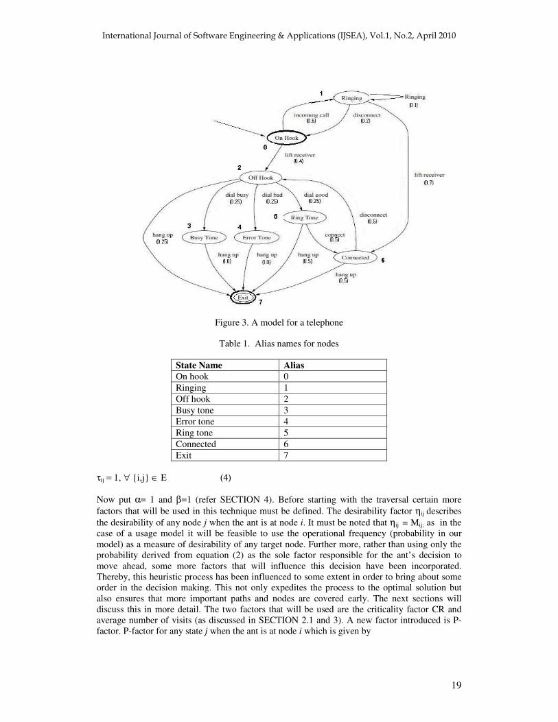
As described in Figure 2 the technique starts with calculating the average visit number of visits of all states (AVi for all i ∈ V) as described in SECTION 3. The telephone model [16] described in Figure 3 will be used henceforth for describing this technique. It is a model for telephone. The model consists of set of nodes V which consists of {ON HOOK}, {RINGING}, {OFF HOOK}, {BUSY TONE}, {ERROR TONE}, {RING TONE}, {CONNECTED}, {EXIT} The exit state is essentially a sink i.e. there are no outgoing transitions from it. The set of transitions or edges as in this case are as follows

{{ON HOOK},{RINGING}}, {{ON HOOK},{OFF HOOK}}, {{RINGING},{ON HOOK}}, {{RINGING},{RINGING}}, {{OFF HOOK},{BUSY TONE}}, {{OFF HOOK},{ERROR TONE}}, {{OFF HOOK},{RING TONE}}, {{RING TONE},{CONNECTED}}, {{CONNECTED},{OFF HOOK}}, {{RINGING},{CONNECTED}}, {{OFF HOOK},{EXIT}}, {{BUSY TONE},{EXIT}}, {{ERROR TONE},{EXIT}}, {{RING TONE},{EXIT}}, {{CONNECTED},{EXIT}}

Now for convenience sake, state names will be substituted with aliases as described in Table 1. The transitional probabilities along the transitional stimuli have been tabulated in Table 2. In order to implement this model a matrix M (n x n) is used, where n is number of nodes. Each Mij in the matrix, is the value of the probability of the transition from node i to j. If no such transition exists, the value is 0. Now we start implementing ant colony optimization to the graph to obtain test sequences. The pheromone levels on all edges are initialised to a value of 1.

������������������� �� ������������������������������������������������������

19

Figure 3. A model for a telephone

Table 1. Alias names for nodes

State Name Alias On hook 0 Ringing 1 Off hook 2 Busy tone 3 Error tone 4 Ring tone 5 Connected 6 Exit 7

τij = 1, ∀ {i,j} ∈ Ε (4)

Now put α= 1 and β=1 (refer SECTION 4). Before starting with the traversal certain more factors that will be used in this technique must be defined. The desirability factor ηij describes the desirability of any node j when the ant is at node i. It must be noted that ηij = Mij; as in the case of a usage model it will be feasible to use the operational frequency (probability in our model) as a measure of desirability of any target node. Further more, rather than using only the probability derived from equation (2) as the sole factor responsible for the ant’s decision to move ahead, some more factors that will influence this decision have been incorporated. Thereby, this heuristic process has been influenced to some extent in order to bring about some order in the decision making. This not only expedites the process to the optimal solution but also ensures that more important paths and nodes are covered early. The next sections will discuss this in more detail. The two factors that will be used are the criticality factor CR and average number of visits (as discussed in SECTION 2.1 and 3). A new factor introduced is P-factor. P-factor for any state j when the ant is at node i which is given by

������������������� �� ������������������������������������������������������

20

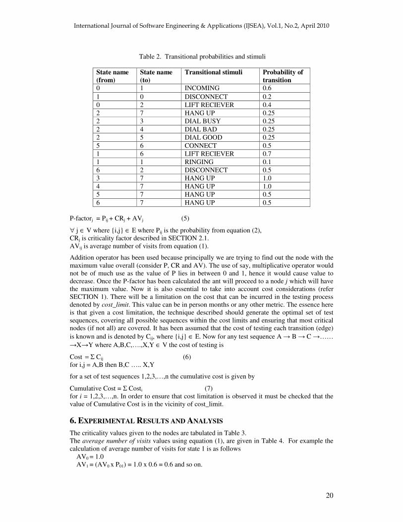
Table 2. Transitional probabilities and stimuli

State name (from)

State name (to)

Transitional stimuli Probability of transition

0 1 INCOMING 0.6 1 0 DISCONNECT 0.2 0 2 LIFT RECIEVER 0.4 2 7 HANG UP 0.25 2 3 DIAL BUSY 0.25 2 4 DIAL BAD 0.25 2 5 DIAL GOOD 0.25 5 6 CONNECT 0.5 1 6 LIFT RECIEVER 0.7 1 1 RINGING 0.1 6 2 DISCONNECT 0.5 3 7 HANG UP 1.0 4 7 HANG UP 1.0 5 7 HANG UP 0.5 6 7 HANG UP 0.5

P-factorj = Pij + CRj + AVj (5)

∀ j ∈ V where {i,j} ∈ Ε where Pij is the probability from equation (2), CRj is criticality factor described in SECTION 2.1. AVij is average number of visits from equation (1).

Addition operator has been used because principally we are trying to find out the node with the maximum value overall (consider P, CR and AV). The use of say, multiplicative operator would not be of much use as the value of P lies in between 0 and 1, hence it would cause value to decrease. Once the P-factor has been calculated the ant will proceed to a node j which will have the maximum value. Now it is also essential to take into account cost considerations (refer SECTION 1). There will be a limitation on the cost that can be incurred in the testing process denoted by cost_limit. This value can be in person months or any other metric. The essence here is that given a cost limitation, the technique described should generate the optimal set of test sequences, covering all possible sequences within the cost limits and ensuring that most critical nodes (if not all) are covered. It has been assumed that the cost of testing each transition (edge) is known and is denoted by Cij, where {i,j} ∈ Ε. Now for any test sequence A � B � C �…… �X�Y where A,B,C,….,X,Y ∈ V the cost of testing is

Cost = Σ Cij (6) for i,j = A,B then B,C ….. X,Y

for a set of test sequences 1,2,3,…,n the cumulative cost is given by

Cumulative Cost = Σ Costi (7) for i = 1,2,3,…,n. In order to ensure that cost limitation is observed it must be checked that the value of Cumulative Cost is in the vicinity of cost_limit.

6. EXPERIMENTAL RESULTS AND ANALYSIS The criticality values given to the nodes are tabulated in Table 3. The average number of visits values using equation (1), are given in Table 4. For example the calculation of average number of visits for state 1 is as follows

AV0 = 1.0 AV1 = (AV0 x P01) = 1.0 x 0.6 = 0.6 and so on.

������������������� �� ������������������������������������������������������

21

Table 3. Criticality values

Node (state) Criticality 0 9.0 1 8.0 2 10.0 3 30.0 4 26.0 5 27.0 6 45.0 7 0.0

Table 4. Average number of visits

Node (state) Average visits 0 1.0 1 0.6 2 0.635 3 0.1 4 0.1 5 0.1 6 0.47 7 0.0

Now as the ant approaches from node to make the first decision i.e. either {0,1} or {0,2}, it is assumed that this decision is random. Ant colony optimization has been avoided at this stage in order to avoid bias towards any branch of the graph emanating from this start state. Any branch emanating from this point carrying a very critical state could force the ants to move over this same path over and over again leaving other less critical paths unvisited for a long time (eventually they will be covered in any case). Once the ant makes this first decision it makes calculations of the P-factors of all nodes immediately reachable from the current node and as described above makes the traversal to the node with the maximum P-factor. Now many such ants are consequently made to traverse the graph. Each leaves its own pheromone trail and hence guides the subsequent ants to the optimal paths. The pheromone levels are updated periodically according to equation (3). Figure 4 shows three paths obtained by three ants in their traversals. Each path is essentially a test sequence. As the test sequences are being generated the Cumulative Cost (equation (7)) is simultaneously calculated. The moment it approaches or exceeds the cost_limit the process is stopped. Once it has been ensured that all the critical nodes and their attached transitions have been covered in the test sequences, the subsequent traversals focus on covering the unvisited nodes and edges giving them a priority over visited, yet more critical nodes (with a higher P-factor). This has been done to ensure complete coverage as long as the cost limitations allow it. In this example it is clear the most critical states (refer Table 3) are 3, 4, 5 and 6. A sample traversal (see test sequence-1 Figure 4) of the model using proposed technique is given below.

The ant starts at start state 0. Say the random decision taken is to go ahead to state 2. So the status of current sequence is 0 � 2. At state 2 the ant has to calculate the P-factor values of all the states that can be reached from 2 in one transition. Namely, these states are 3, 4, 5and 7. The P-factor values calculated is as follow. Using equation (5) for P-factor

������������������� �� ������������������������������������������������������

22

Figure 4. Illustration of some of the test sequences covered

P-factor3 = P23 + CR3 + AV3 = 30.138 Where, P23 = {(τij)α x (ηij)β } / Σ (τij)α x (ηij)β = {(1.0)1 x (0.25)2} /6.5 = 0.3824

Putting these values in equation (2)

CR3 = 30.0 from Table 2

AV3 = 0.1 from Table 3

Similarly, P-factor4 = P24 + CR4 + AV4 = 26.138 P-factor5 = P25 + CR5 + AV5 = 27.138 P-factor7 = P27 + CR7 + AV7 = 0.0384 Hence the ant selects state 3 for next transition. The test sequence till now is 0 � 2 � 3. At state 3 the only transition possible is {3,7}. Final test sequence generated is 0 � 2 � 3 � 7.

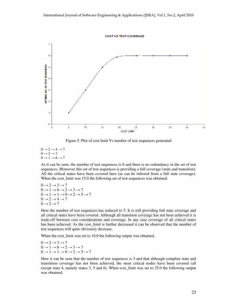
Following are some of the outputs obtained at various cost_limit values. In each of the following obtained outputs, the number of critical states covered will be checked. This is done in order to verify whether the critical states are being covered even under very strict cost limitations. The following test sequences were obtained when cost_limit was 20.0.

0 � 2 � 3 � 7 0 � 1 � 6 � 2 � 3 � 7 0 � 1 � 1 � 0 � 2 � 5 � 7

������������������� �� ������������������������������������������������������

23

Figure 5. Plot of cost limit Vs number of test sequences generated

0 � 2 � 4 � 7 0 � 2 � 7 0 � 1 � 6 � 7

As it can be seen, the number of test sequences is 6 and there is no redundancy in the set of test sequences. Moreover this set of test sequences is providing a full coverage (state and transition). All the critical states have been covered here (as can be inferred from a full state coverage). When the cost_limit was 15.0 the following set of test sequences was obtained.

0 � 2 � 3 � 7 0 � 1 � 6 � 2 � 3 � 7 0 � 1 � 1 � 0 � 2 � 5 � 7 0 � 2 � 4 � 7 0 � 2 � 7

Here the number of test sequences has reduced to 5. It is still providing full state coverage and all critical states have been covered. Although all transition coverage has not been achieved it is trade-off between cost considerations and coverage. In any case coverage of all critical states has been achieved. As the cost_limit is further decreased it can be observed that the number of test sequences will quite obviously decrease.

When the cost_limit was set to 10.0 the following output was obtained.

0 � 2 � 3 � 7 0 � 1 � 6 � 2 � 3 � 7 0 � 1 � 1 � 0 � 2 � 5 � 7

Here it can be seen that the number of test sequences is 3 and that although complete state and transitions coverage has not been achieved, the most critical nodes have been covered (all except state 4, namely states 3, 5 and 6). When cost_limit was set to 25.0 the following output was obtained.

������������������� �� ������������������������������������������������������

24

Figure 6. Plot of cost limit Vs number of critical nodes covered

0 � 2 � 3 � 7 0 � 1 � 6 � 2 � 3 � 7 0 � 1 � 1 � 0 � 2 � 5 � 7 0 � 2 � 4 � 7 0 � 2 � 7 0 � 1 � 6 � 7

It is evident that this is same result as when the limit was 20.0. Similar results were obtained when the cost_limit was set to values above 25.0. So it can be inferred that after a certain threshold value of cost_limit the there is no change in the output and that further cost investment is not required. The optimal test sequence set (giving full coverage) is obtained at a certain threshold value. A similar trend is seen in case of number of critical nodes covered. In Figure 4 and 5 the cost_limit has been plotted versus the number of test sequences and the number of critical nodes covered. It is clearly visible that after the threshold value of 20.0 the curve is a constant.

7. COMPARISON WITH EXISTING TECHNIQUES Li and Lam [20] have worked on the use of Ant colony optimization in test sequence generation in a state based approach to testing. But the work does not factor in criticality of the states or give conclusively optimized test sequences. A comparative study has been made using results obtained by applying the above mention technique [20] and the proposed technique. This work has been chosen for a comparative study because as per our research this is the only work that incorporates ACO in model based testing, and the purpose of this comparative study is to prove that a markov chain usage model is better than a simple state based model for the application of ACO. An equal number of test sequences are generated by both the techniques. These are test sequences generated by traversals by equal number of ants. The comparative study has been made on the basis of the number of nodes and edges covered in the same number of traversals. The n test sequences considered here are derived from the first n traversals of the model. This

������������������� �� ������������������������������������������������������

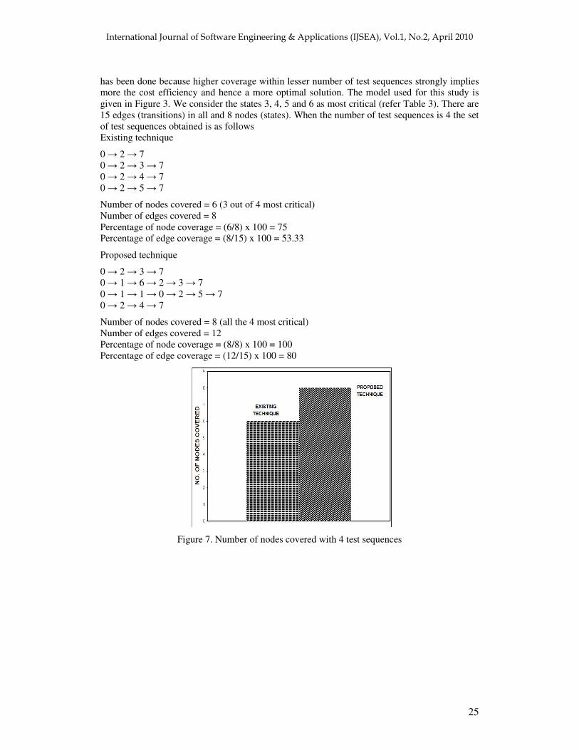
25

has been done because higher coverage within lesser number of test sequences strongly implies more the cost efficiency and hence a more optimal solution. The model used for this study is given in Figure 3. We consider the states 3, 4, 5 and 6 as most critical (refer Table 3). There are 15 edges (transitions) in all and 8 nodes (states). When the number of test sequences is 4 the set of test sequences obtained is as follows Existing technique

0 � 2 � 7 0 � 2 � 3 � 7 0 � 2 � 4 � 7 0 � 2 � 5 � 7

Number of nodes covered = 6 (3 out of 4 most critical) Number of edges covered = 8 Percentage of node coverage = (6/8) x 100 = 75 Percentage of edge coverage = (8/15) x 100 = 53.33

Proposed technique

0 � 2 � 3 � 7 0 � 1 � 6 � 2 � 3 � 7 0 � 1 � 1 � 0 � 2 � 5 � 7 0 � 2 � 4 � 7

Number of nodes covered = 8 (all the 4 most critical) Number of edges covered = 12 Percentage of node coverage = (8/8) x 100 = 100 Percentage of edge coverage = (12/15) x 100 = 80

Figure 7. Number of nodes covered with 4 test sequences

������������������� �� ������������������������������������������������������

26

Figure 8. Number of edges covered with 4 test sequences

Figure 7 and Figure 8 show a graph describing the results obtained above. When the number of test sequences is 4 the set of test sequences obtained is as follows

Existing technique

0 � 2 � 7 0 � 2 � 3 � 7

Number of nodes covered = 4 (1 out of 4 most critical) Number of edges covered = 3 Percentage of node coverage = (4/8) x 100 = 50 Percentage of edge coverage = (3/15) x 100 = 20

Proposed technique

0 � 2 � 3 � 7 0 � 1 � 6 � 2 � 3 � 7

Number of nodes covered = 6 (2 out of 4 most critical) Number of edges covered = 6 Percentage of node coverage = (6/8) x 100 = 75 Percentage of edge coverage = (6/15) x 100 = 40

Figure 9. Number of nodes covered with 2 test sequences

������������������� �� ������������������������������������������������������

27

Figure 10. Number of edges covered with 2 test sequences

Figure 9 and Figure 10 show a graph describing the results obtained above. It is quite evident that the proposed technique not only ensures a better coverage but also ensures that the more critical states are covered too. Doerner and Gutjahr [11] have used Ant colony optimization to generate test sequences from markov chain based models. But the technique described [11] does not take the criticality of the states into account. The technique proposed in this paper uses criticality of state explicitly as well computes its own measure (average number of visits) to gauge the criticality of any state. It gives better coverage of critical nodes, especially when there are strict cost limitations. Under such conditions although a lesser number of test sequences are generated, the set is optimal for that given cost. This is a very desirable result.

8. CONCLUSIONS The above discussed technique has proven to be effective in generating optimal set of test cases from a markov chain based usage model. Especially with the growth in software with extensive graphical interfaces, usage modelling will prove to be very fruitful. The technique takes into account the average number of visits to any state; this is a very important factor when testing graphical interfaces. The discussed technique has also proved to be capable of deriving test cases with priority given to the most critical states and transitions. Even with strict cost limitations it has been observed that the most critical states have been covered. Future works upon this technique could involve the presence of multiple transitional probabilities between states [6]. The use of ant colony optimization has proven to be effective and provides an efficient means to generate test sequences especially in graph based models. The complexity of algorithm used in this technique is O (n2) for a traversal and hence proves to be efficient and less computation intensive.

REFERENCES [1] R. Pressman (2001) Software Engineering – A Practitioner’s Approach. 5th edition. New York,

NY: McGraw Hill.

[2] M. Utting and B. Legeard (2007) Practical Model Based Testing – A tools approach. San Francisco, CA: Morgan Kaufmann.

[3] G. J. Myers (1979) The Art of Software Testing. New York: Wiley

[4] D. M. Woit, (1992) “Realistic expectations of random testing”, CRL Rep. 246, McMaster Univ., Hamilton, ON, Canada.

[5] J. Keilson (1979) Markov Chain Models; Rarity and Exponentiality. New York, NY: Springer-Verlag.

������������������� �� ������������������������������������������������������

28

[6] J. A. Whittaker and M. G. Thomason, (1994) “A markov chain model for statistical software testing”, IEEE Transactions on Software Engineering, vol. 20, no. 10, pp. 812-824.

[7] J.A. Whittaker and J. H. Poore, (1993) “Markov analysis of software specifications”, ACM Tran. Software Eng. Methodology, vol. 2, no. 1, pp. 93-106.

[8] G. Walton, J. Poore, C. Trammell, (1995) “Statistical testing of software based on a usage model”, Software: Practice and Experience, vol. 25, no. 1, pp. 97-108.

[9] J. A. Whittaker, (1992) “Markov chain techniques for software testing and reliability analysis”, Ph.D. dissertation, Dept. of Comput. Sci., Univ. of Tennessee, Knoxville, USA.

[10] S. J. Prowell, (2005) “Using markov chain usage models to test complex systems”, Proceedings of the 38th Annual Hawaii International Conference on System Sciences (HICSS'05), vol. 9, pp.318c, track 9.

[11] K. Doerner and W. J. Gutjahr, (2003) “Extracting test sequences from a markov software usage model by ACO”, GECCO 2003, LNCS, vol. 2724, pp. 2465-2476.

[12] K. Mark and L. Csaba, (2007) “Analysing customer behaviour model graph (CBMG) using markov chains”, 11th International Conference on Intelligent Engineering Systems, 2007. INES 2007, pp. 71-76.

[13] S. J. Prowell, (2003) Computations for Markov Chain Usage Models, Computer Science Technical Report UT-CS-03- 505, The University of Tennessee, Knoxville, TN, USA.

[14] K. D. Sayre, (1999) “Improved Techniques for Software Testing Based on Markov Chain Usage Models”, PhD thesis, The University of Tennessee, Knoxville, TN, USA.

[15] J. E. Hopcroft and J. D. Ullman (1979) Introduction to Automata Theory, Languages, and Computation, Reading, MA: Addison-Wesley.

[16] S. J. Prowell, (2003) “JUMBL: A Tool for Model-Based Statistical Testing”, at 36th Annual Hawaii International Conference on System Sciences (HICSS'03), HICSS, vol. 9, pp.337c, Track 9.

[17] M. Dorigo, V. Maniezzo, and A. Colorni (1991) The Ant System: An Autocatalytic Optimizing Process, Technical Report TR91-016, Politecnico di Milano.

[18] A. Colorni, M. Dorigo, and V. Maniezzo, (1991) “Distributed optimization by ant colonies”, Proceedings of ECAL'91, European Conference on Artificial Life, Elsevier Publishing, Amsterdam.

[19] M. Dorigo and G. Di Caro, (1999) “The Ant colony optimization meta-heuristic”, in D. Corne, M. Dorigo and F. Glover, editors, New Ideas in Optimization, McGraw-Hill, pp. 11-32.

[20] H. Li and C. P. Lam, (2004) “Software Test Data Generation using Ant Colony Optimization”, International Conference of Computational Intelligence, pp. 1-4.