1/25

Optimized Ogata quadrature andapplications to the Sivers Asymmetry

John Terry

University of California, Los Angeles

QCD Evolution WorkshopArgonne National Lab

May 15, 2019

2/25

Fit to Sivers asymmetry done in collaboration with

Miguel Echevarriaand Zhongbo Kang.

Optimized Ogata method is done in collaboration with

Zhongbo Kang,Alexei Prokudin,and Nobuo Sato.

3/25

Overview

1 Introduction to the Sivers Asymmetry

2 TMD Formalism for Sivers Asymmetry

3 Why we need high efficiency Fourier transforms

4 Preliminary Fit Results

5 Conclusions

4/25

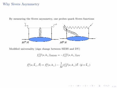
Why Sivers Asymmetry

By measuring the Sivers asymmetry, one probes quark Sivers functions

Modified universality (sign change between SIDIS and DY)

f⊥q1T (x, k⊥)|SIDIS = −f⊥q1T (x, k⊥)|DY

fq1 (x,~k⊥, ~S) = fq1 (x, k⊥)−1

Mf⊥q1T (x, k⊥)~S · (p× ~k⊥)

5/25

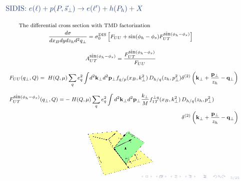
SIDIS: e(`) + p(P,~s⊥) → e(`′) + h(Ph) + X

The differential cross section with TMD factorization

dσ

dxBdydzhd2q⊥= σDIS

0

[FUU + sin(φh − φs)F

sin(φh−φs)UT

]

Asin(φh−φs)UT =

Fsin(φh−φs)UT

FUU

FUU (q⊥, Q) = H(Q,µ)∑q

e2q

∫d2k⊥d

2p⊥fq/p(xB , k2⊥)Dh/q(zh, p

2⊥)δ(2)

(k⊥ +

p⊥zh− q⊥

)

Fsin(φh−φs)UT (q⊥, Q) = − H(Q,µ)

∑q

e2q

∫d2k⊥d

2p⊥k⊥Mf⊥q1T (xB , k

2⊥)Dh/q(zh, p

2⊥)

δ(2)

(k⊥ +

p⊥zh− q⊥

)

6/25

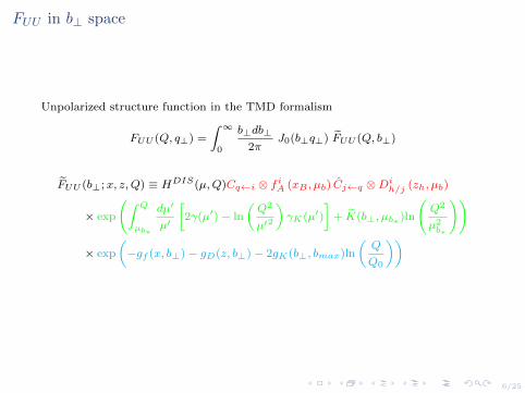
FUU in b⊥ space

Unpolarized structure function in the TMD formalism

FUU (Q, q⊥) =

∫ ∞0

b⊥db⊥2π

J0(b⊥q⊥) FUU (Q, b⊥)

FUU (b⊥;x, z,Q) ≡ HDIS(µ,Q)Cq←i ⊗ f iA (xB , µb) Cj←q ⊗Dih/j (zh, µb)

× exp

(∫ Q

µb∗

dµ′

µ′

[2γ(µ′)− ln

(Q2

µ′2

)γK(µ′)

]+ K(b⊥, µb∗ )ln

(Q2

µ2b∗

))

× exp

(−gf (x, b⊥)− gD(z, b⊥)− 2gK(b⊥, bmax)ln

(Q

Q0

))

7/25

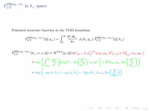
F sinφh−φsUT in b⊥ space

Polarized structure function in the TMD formalism

Fsin(φh−φs)UT (Q, q⊥) =

∫ ∞0

b2⊥db⊥

4πJ1(b⊥q⊥) F

sin(φh−φs)UT (Q, b⊥)

Fsin(φh−φs)UT (b⊥;x, z,Q) ≡ HDIS(µ,Q)∆Cq←i ⊗ f

⊥(1)1T (xB , µb∗ )Cj←q ⊗Dih/j (zh, µb∗ )

× exp

(∫ Q

µb∗

dµ′

µ′

[2γ(µ′)− ln

(Q2

µ′2

)γK(µ′)

]+ K(b⊥, µb∗ )ln

(Q2

µ2b∗

))

× exp

(−gT (x, b⊥)− gD(z, b⊥)− 2gK(b⊥, bmax)ln

(Q

Q0

))

8/25

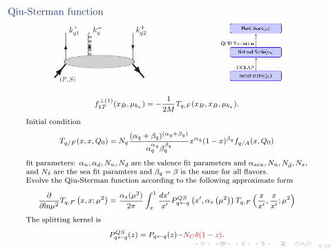
Qiu-Sterman function

f⊥(1)1T (xB , µb∗ ) = −

1

2MTq,F (xB , xB , µb∗ ).

Initial condition

Tq/F (x, x,Q0) = Nq(αq + βq)(αq+βq)

ααqq β

βqq

xαq (1− x)βqfq/A(x,Q0)

fit parameters: αu, αd, Nu, Nd are the valence fit parameters and αsea, Nu, Nd, Ns,and Ns are the sea fit paramters and βq = β is the same for all flavors.Evolve the Qiu-Sterman function according to the following approximate form

∂

∂lnµ2Tq,F

(x, x;µ2

)=αs(µ2)

2π

∫ 1

x

dx′

x′PQSq←q

(x′, αs

(µ2))Tq,F

( xx′,x

x′;µ2)

The splitting kernel is

PQSq←q(z) = Pq←q(z)−NCδ(1− z).

9/25

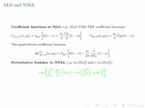
NLO and NNLL

Coefficient functions at NLO, e.g., NLO TMD PDF coefficient functions

Cq←q′ (x, µb) = δqq′

[δ(1− x) +

αs

π

CF

2(1− x)

]Cq←g(x, µb) =

αs

πTRx(1− x) .

The quark-Sivers coefficient function

∆CTq←q′ (x, µb) = δqq′

[δ(1− x)−

αs

2π

1

4NC(1− x)

]Perturbative Sudakov to NNLL (γK to O(α3

s) and γ to O(α2s))

exp

(∫ Q

µb∗

dµ′

µ′

[2γ(µ′)− ln

(Q2

µ′2

)γK(µ′)

])

10/25

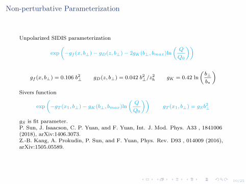
Non-perturbative Parameterization

Unpolarized SIDIS parameterization

exp

(−gf (x, b⊥)− gD(z, b⊥)− 2gK(b⊥, bmax)ln

(Q

Q0

))

gf (x, b⊥) = 0.106 b2⊥ gD(z, b⊥) = 0.042 b2⊥/z2h gK = 0.42 ln

(b⊥b∗

)Sivers function

exp

(−gT (x1, b⊥)− gK(b⊥, bmax)ln

(Q

Q0

))gT (x1, b⊥) = gSb

2⊥

gS is fit parameter.P. Sun, J. Isaacson, C. P. Yuan, and F. Yuan, Int. J. Mod. Phys. A33 , 1841006(2018), arXiv:1406.3073.Z.-B. Kang, A. Prokudin, P. Sun, and F. Yuan, Phys. Rev. D93 , 014009 (2016),arXiv:1505.05589.

11/25

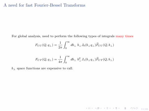
A need for fast Fourier-Bessel Transforms

For global analysis, need to perform the following types of integrals many times

FUU (Q, q⊥) =1

2π

∫ ∞0

db⊥ b⊥J0(b⊥q⊥)FUU (Q, b⊥)

FUT (Q, q⊥) =1

4π

∫ ∞0

db⊥ b2⊥J1(b⊥q⊥)FUT (Q, b⊥)

b⊥ space functions are expensive to call.

12/25

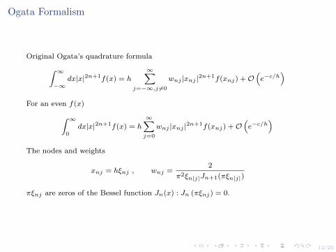
Ogata Formalism

Original Ogata’s quadrature formula∫ ∞−∞

dx|x|2n+1f(x) = h∞∑

j=−∞,j 6=0

wnj |xnj |2n+1f(xnj) +O(e−c/h

)For an even f(x)∫ ∞

0dx|x|2n+1f(x) = h

∞∑j=0

wnj |xnj |2n+1f(xnj) +O(e−c/h

)The nodes and weights

xnj = hξnj , wnj =2

π2ξn|j|Jn+1(πξn|j|)

πξnj are zeros of the Bessel function Jn(x) : Jn (πξnj) = 0.

13/25

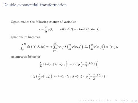
Double exponential transformation

Ogata makes the following change of variables

x =π

hψ(t) with ψ(t) = t tanh

(π2

sinh t)

Quadrature becomes∫ ∞0

dxf(x) Jn(x) ≈ πN∑j=1

wnj f(πhψ(xnj)

)Jn(πhψ(xnj)

)ψ′(xnj),

Asymptotic behavior

π

hψ (hξnj) ≈ πξnj

[1− 2 exp

(−π

2ehξnj

)]

Jn(πhψ(xnj)

)≈ 2πξnjJn+1(πξnj) exp

(−π

2ehξnj

).

14/25

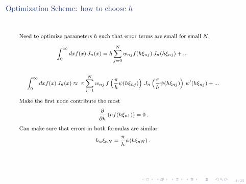
Optimization Scheme: how to choose h

Need to optimize parameters h such that error terms are small for small N .∫ ∞0

dxf(x) Jn(x) = hN∑j=0

wnjf(hξnj) Jn(hξnj) + ...

∫ ∞0

dxf(x) Jn(x) ≈ πN∑j=1

wnj f(πhψ(hξnj)

)Jn(πhψ(hξnj)

)ψ′(hξnj) + ...

Make the first node contribute the most

∂

∂h(hf(hξn1)) = 0 ,

Can make sure that errors in both formulas are similar

huξnN =π

hψ(hξnN ) .

15/25

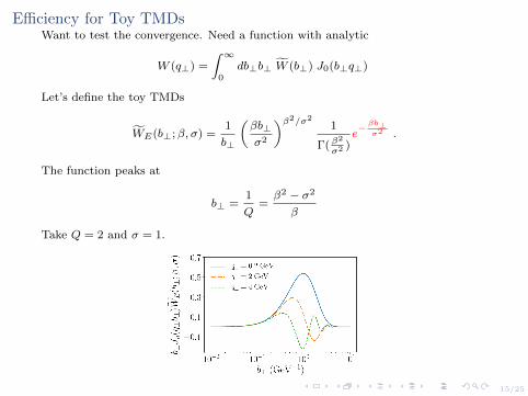
Efficiency for Toy TMDsWant to test the convergence. Need a function with analytic

W (q⊥) =

∫ ∞0

db⊥b⊥ W (b⊥) J0(b⊥q⊥)

Let’s define the toy TMDs

WE(b⊥;β, σ) =1

b⊥

(βb⊥σ2

)β2/σ21

Γ(β2

σ2 )e− βb⊥

σ2 .

The function peaks at

b⊥ =1

Q=β2 − σ2

β

Take Q = 2 and σ = 1.

16/25

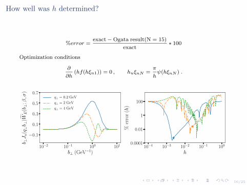
How well was h determined?

%error =exact−Ogata result(N = 15)

exact∗ 100

Optimization conditions

∂

∂h(hf(hξn1)) = 0 , huξnN =

π

hψ(hξnN ) .

10−2 10−1 100 101

b⊥ (GeV−1)

−0.1

0.1

0.3

0.5

0.7

b ⊥Jn(q⊥b ⊥

)WE

(b⊥

;β,σ

)

q⊥ = 0.2 GeV

q⊥ = 2 GeV

q⊥ = 4 GeV

10−4 10−3 10−2 10−1 100

h

100

1

0.01

0.0001

%er

ror

(h)

17/25

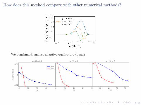
How does this method compare with other numerical methods?

We benchmark against adaptive quadrature (quad)

10 20 30 40N

0.01

1

100

%er

ror

(N)

q⊥/Q = 0.1

quad

ogata

10 20 30 40N

q⊥/Q = 1

10 30 50 70 90N

q⊥/Q = 2

18/25

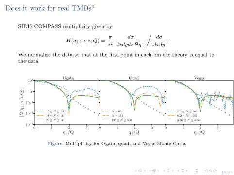
Does it work for real TMDs?

SIDIS COMPASS multiplicity given by

M(q⊥;x, z,Q) =π

z2

dσ

dxdydzd2q⊥

/dσ

dxdy,

We normalize the data so that at the first point in each bin the theory is equal tothe data

0 1 2 3

q⊥/Q

10−3

10−2

10−1

100

101

|M(q⊥

;x,z,Q

)|

Ogata

15 ≤ N ≤ 27

18 ≤ N ≤ 30

28 ≤ N ≤ 40

0 1 2 3

q⊥/Q

Quad

N = 65

N = 135

135 ≤ N ≤ 860

0 1 2 3

q⊥/Q

Vegas

231 ≤ N ≤ 263

602 ≤ N ≤ 657

3937 ≤ N ≤ 4054

Figure: Multiplicity for Ogata, quad, and Vegas Monte Carlo.

19/25

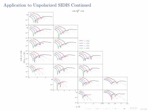
Application to Unpolarized SIDIS Continued

10−4

10−2

100

=⇒ Q2 =⇒

10−4

10−2

100

10−4

10−2

100 z =0.2

z =0.3

z =0.4

z =0.6

10−4

10−2

100

|M(q⊥

;x,z,Q

)|=⇒

x=⇒

0 2 4 610−4

10−2

100

0 1 2 3 410−4

10−2

100

0 1 2 3

q⊥/Q

10−4

10−2

100

0.0 0.5 1.0 1.5 2.0

Figure: Comparison of COMPASS multiplicities [?].

20/25

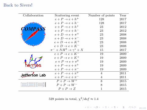
Back to Sivers!

Collaboration Scattering event Number of points Yeare+ P → e+ h+ 128 2017e+ P → e+ h− 128 2017e+ P → e+ h+ 23 2012e+ P → e+ h− 23 2012e+D → e+ π+ 23 2008e+D → e+ π− 23 2008e+D → e+K+ 23 2008e+D → e+K− 23 2008

π− +NH3 → γ∗ +X 15 2017e+ P → e+K− 19 2009e+ P → e+K+ 19 2009e+ P → e+ π0 19 2009e+ P → e+ π+ 19 2009e+ P → e+ π− 19 2009e+ P → e+ π+ 4 2011e+ P → e+ π− 4 2011P + P →W+ 8 2015P + P →W− 8 2015P + P → Z 1 2015

529 points in total, χ2/dof ≈ 1.4

21/25

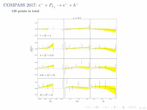
COMPASS 2017: e− + Ps⊥ → e− + h−

128 points in total

−0.05

0.00

0.05

1 < Q2 < 4

z > 0.1

−0.05

0.00

0.05

AS

iver

sU

T

4 < Q2 < 6.25

−0.05

0.00

0.05

6.25 < Q2 < 16

0.25 0.50 0.75 1.00 1.25

p⊥

−0.05

0.00

0.05

16 < Q2 < 81

0.2 0.4 0.6

xB

0.2 0.4 0.6

zh

22/25

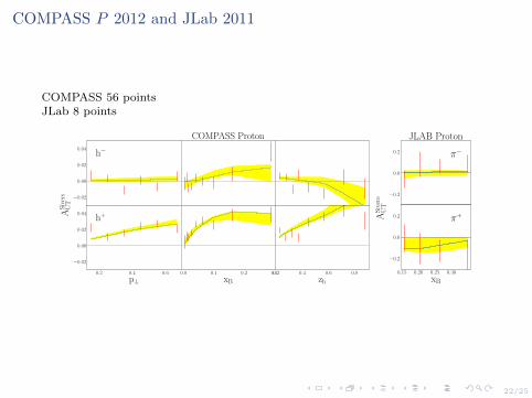
COMPASS P 2012 and JLab 2011

COMPASS 56 pointsJLab 8 points

−0.02

0.00

0.02

0.04

AS

iver

sU

T

h−

COMPASS Proton

0.2 0.4 0.6

p⊥

−0.02

0.00

0.02

0.04h+

0.0 0.1 0.2 0.3

xB

0.2 0.4 0.6 0.8

zh

xB

−0.2

0.0

0.2

AS

iver

sU

T

JLAB Proton

π−

0.15 0.20 0.25 0.30

xB

−0.2

0.0

0.2 π+

23/25

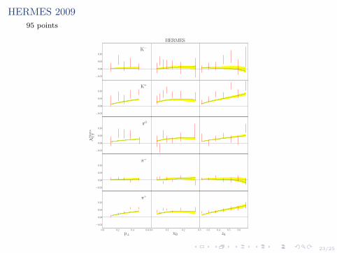
HERMES 2009

95 points

−0.05

0.00

0.05

0.10

K−

HERMES

−0.05

0.00

0.05

0.10

K+

−0.05

0.00

0.05

0.10

AS

iver

sU

T

π0

−0.05

0.00

0.05

0.10

π−

0.0 0.2 0.4 0.6

p⊥

−0.05

0.00

0.05

0.10

π+

0.0 0.1 0.2 0.3

xB

0.3 0.4 0.5 0.6

zh

24/25

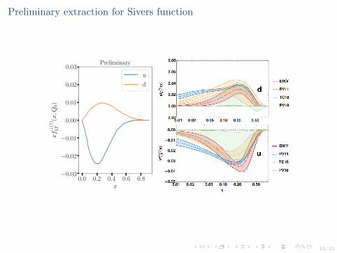
Preliminary extraction for Sivers function

0.0 0.2 0.4 0.6 0.8x

−0.03

−0.02

−0.01

0.00

0.01

0.02

0.03

xf⊥

(1)

1T(x,Q

0)

Preliminary

u

d

25/25

Conclusion

• We generated an optimized Ogata method, highly numerically efficient

• The method can be used for global analysis

• Ogata algorithm will be available open source in the future

• We can use the NLO/NNLL parameterization to describe SIDIS Sivers data

• We hope to soon describe the DY and vector boson data

Thanks!!