THE COOPER UNION FOR THE ADVANCEMENT OF SCIENCE AND ART

OPTIMIZATION OF THE RISE TIME FOR A SECONDORDER PITCH RATE CONTROL SYSTEM

"Group 2"

Advisors: Benjamin Davis, Hamid Ahmad CHE 488/ Fall 2011

1

I. ABSTRACT

This paper describes the tuning of an optimal proportional-integral (PI) controller to minimizerise time for an airplane pitch rate control system. The pitch rate control system, along withthe yaw and roll control systems, make up the backbone of an airplane flight control system.We present the transfer function of the system and impose stability constraints using Routh-Hurwitz tabulation. We must also impose constraints so that the system may be approximated asa standard form second order system, so that a closed-form rise time expression from Ogata [1]can be used. We rigorously prove that the objective function has a minimum over the feasible set.We design the optimal controller is designed using Matlab; the solution could be implementedas part of any airplane flight control system where the pitch dynamics can be modeled as firstorder.

2

II. INTRODUCTION

In aircraft flight systems, the primary concern is control over the principal axes: yaw, pitch,and roll to ensure a stable flight path. These axes are shown in Figure 1. Our focus in thispaper is the pitch rate control system. A control system is a system which attempts to maintaina quantity (or quantities) in a specified operating range. In a pitch rate control system, the pilotsets a desired pitch rate, and the system responds by adjusting the actual aircraft pitch rate.

Fig. 1: Diagram which illustrates principal axes of aircraft motion, from [2]

As this problem is a standard one present in nearly every aircraft flight control system, a vastnumber of controlling methods have been explored, for example [3], [4]. Pitch rate controllershave been implemented by using fuzzy controls [5], neural networks [6], and sliding modecontrol methods [7]. This project uses a PI controller, as implemented in a pitch rate controlsystem by [8].

PI controllers are used in a wide range of applications, but they are inherently linear and non-adaptive. As shown in [9], PI controller design based purely on system models gives generally“poor performance,” unless they are retuned with flight test data. A more advanced and suitablePI controller is adaptive in nature [10]. Therefore, for proper application of our optimal solutionusing a linear non-adaptive PI controller, the controller will need to be adjusted and verifiedwith flight test data. Simulations using a “crewed flight simulator” would also assist in adjustingthe controller and verifying functionality [11].

As our system is linear and time invariant (LTI), LTI theory can be applied to develop a systemmodel. Any LTI system can be completely characterized by its impulse response function. Theimpulse response g(t) is given by g(t) = c(t)|r(t)=δ(t), where c(t) is the output of the system,r(t) is the input to the system, and δ(t) denotes the dirac delta function. The impulse responsecan be used to determine the system response for any input r(t):

c(t) = g(t) ? r(t) (1)

where ? denotes convolution.

3

Because convolution computations can be tedious, we apply the Laplace transform to Equation(1) to transform from the time domain to the Laplace domain. The convolution in the time domainmaps to multiplication in the Laplace domain [1]:

L [c(t) = g(t) ? r(t)]

C(s) = G(s)R(s) (2)

G(s) in Equation (2) is defined as the transfer function of the system. Now, given any input inthe time domain, we apply the Laplace transform and multiply it with our transfer function tofind the response in the Laplace domain. By taking the inverse Laplace transform of this quantity,the response in the time domain can be obtained. This process is equivalent to convolving theinput in the time domain with the impulse response of the system.

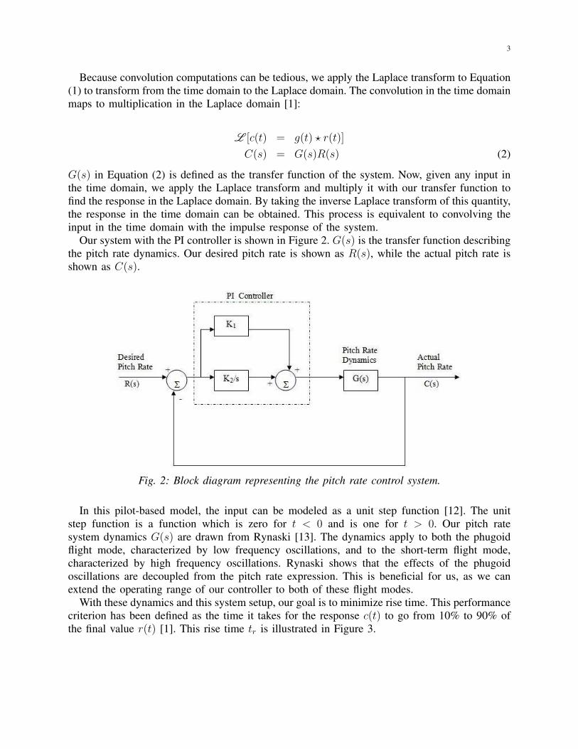
Our system with the PI controller is shown in Figure 2. G(s) is the transfer function describingthe pitch rate dynamics. Our desired pitch rate is shown as R(s), while the actual pitch rate isshown as C(s).

Fig. 2: Block diagram representing the pitch rate control system.

In this pilot-based model, the input can be modeled as a unit step function [12]. The unitstep function is a function which is zero for t < 0 and is one for t > 0. Our pitch ratesystem dynamics G(s) are drawn from Rynaski [13]. The dynamics apply to both the phugoidflight mode, characterized by low frequency oscillations, and to the short-term flight mode,characterized by high frequency oscillations. Rynaski shows that the effects of the phugoidoscillations are decoupled from the pitch rate expression. This is beneficial for us, as we canextend the operating range of our controller to both of these flight modes.

With these dynamics and this system setup, our goal is to minimize rise time. This performancecriterion has been defined as the time it takes for the response c(t) to go from 10% to 90% ofthe final value r(t) [1]. This rise time tr is illustrated in Figure 3.

4

Fig. 3: Diagram illustrating rise time tr [1].

III. PROBLEM DESCRIPTION

A zero, z, of a rational function f : C → C is a value such that f(z) = 0. If the Laurentseries of the function f(s) around a singular point p has a principal part that contains at leastone nonzero term, then we call p a pole of f(s) [14].

In general, we can express the transfer function of any second order system that contains nofinite zeros as follows:

Y (s) =ω2n

s2 + 2ζωns+ ω2n

(3)

where ωn is the undamped natural frequency and ζ is the damping ratio of the system [15]. Theseparameters determine the transient response characteristics, including rise time, of a second ordersystem. As described in [1], the rise time of this system due to a unit step input has an analyticalexpression given by:

tr =π − cos−1(ζ)

ωn√1− ζ2

(4)

For this project, the transfer function G(s) we used to model the pitch-rate command systemis given by:

G(s) =20

s+ 4.4, (5)

the model used in the NASA aircraft report [13]. When G(s) is placed in a unity feedback loopwith a PI controller, as shown in Figure 2, the closed loop transfer function of the completepitch-rate control system is given by M(s). For our system, M(s) is given by the followingequation:

M(s) =(K1 +K2/s)G(s)

1 + (K1 +K2/s)G(s)(6)

5

Substituting Equation (5) into Equation (6), M(s) reduces to the following expression:

M(s) =s(20K1) + 20K2

s2 + s(20K1 + 4.4) + 20K2

(7)

We see from Equation (7) that our pitch-rate control system is a secondorder system containingtwo poles and one zero. The transfer function cannot be expressed in the form given by Equation(3) because it contains a finite zero. Therefore, we cannot calculate the rise time of the systemdue to a unit step input directly from Equation (4). However, [16] outlines a procedure forsuppressing the effects of the finite zero on the system’s transient behavior, allowing us toapproximate our system as a second order system with no finite zero. With this approximation,we can calculate the rise time of the system from Equation (4).

The first step of this approximation procedure is to rewrite the transfer function in the form:

M(s) =(s+ α)(ω2

n/α)

s2 + 2ζωns+ ω2n

(8)

where s = −α is the zero of the system. We therefore rewrite Equation (7) as follows:

M(s) =(s+K2/K1)20K1

s2 + s(20K1 + 4.4) + 20K2

(9)

where −α= −K2/K1, 2ζωn = (20K1 + 4.4), and ω2n = 20K2. Solving the latter two equations

for ζ and ωn in terms of K1 and K2 we have:

ζ =20K1 + 4.4

2√20K2

(10)

ωn =√20K2 (11)

In order for the finite zero to be considered insignificant in regards to the transient behavior,the magnitude of the zero must be more than 5 times the magnitude of the real part of thecomplex conjugate poles [16]: ∣∣∣∣−K2

K1

∣∣∣∣ ≥ (5 + ε) |<(Pcomplex)| (12)

Pcomplex is either of the two complex poles of the system, as each have the same real part.Note that we choose the quantity ε > 0 to equal 10−10 in order to have a non-strict inequalityconstraint.

The poles of the system given by Equation (9) are the roots of the denominator D(s):

D(s) = s2 + s(20K1 + 4.4) + 20K2. (13)

From the quadratic formula, we see that −b2a

corresponds to the real part of the roots when theroots are a complex conjugate pair. Therefore we can rewrite Equation (12):∣∣∣∣−K2

K1

∣∣∣∣ ≥ (5 + ε) |−10K1 − 2.2| (14)

As it is not conventional to use the absolute value function when expressing constraints, werewrite the constraint into the following equivalent set:

6

K2

K1

≤ −(5 + ε)(10K1 + 2.2) (15)

K2

K1

≥ (5 + ε)(10K1 + 2.2) (16)

When determining the optimal values of K1 and K2, we must ensure that our system is stablefor our choices of K1 and K2. A system is stable when all the real parts of its poles are lessthan zero [15]. We use the modified Routh-Hurwitz (R-H) stability criterion [1] to determinewhich constraints on K1 and K2 guarantee stability. Rather than allowing poles to exist nearthe imaginary axis, the modified method ensures that the real parts of the poles are less than orequal to -0.5, giving us a larger stability margin [17].

The denominator polynomial given by Equation (13) is used in the stability criterion with thesubstitution s = z − 0.5. After substitution, we obtain:

D(z) = z2 + z(20K1 + 3.4)− 10K1 + 20K2 − 1.95 (17)

The Routh-Hurwitz array of this polynomial is shown below:

(1) (2) (3)z2 1 −10K1 + 20K2 − 1.95 0z1 20K1 + 3.4 0 0z0 −10K1 + 20K2 − 1.95 0 0

In order to satisfy the R-H criterion, all the entries in column (1) must be greater than orequal to zero. This gives us the following constraints on K1 and K2:

20K1 + 3.4 ≥ 0 (18)

−10K1 + 20K2 − 1.95 ≥ 0 (19)

Our final constraint on K1 and K2 is a transient response constraint. Figure 3 shows thetransient response of a second order system due to a unit step input. The rise time and maximumpeak overshoot (Mp) are depicted in the figure. Selection of the damping ratio ζ involves a trade-off between rise time and Mp. A smaller damping ratio decreases the rise time but increasesMp, while increasing the ratio increases the rise time and decreases Mp. A suggested dampingratio range is given by [16]:

0.4 ≤ ζ ≤ 0.7 (20)

Substituting Equation (10) into Equation (20), we have:

0.4 ≤ 20K1 + 4.4

2√20K2

≤ 0.7 (21)

As can be seen in Equation (21), to avoid division by zero and imaginary quantities, we mustimpose an additional constraint on K2:

K2 ≥ ε (22)

7

Our objective function for the optimization problem is given by Equation (4). The constraintsare given by equations (15), (16), (18), (19), and (21).

minimizeK1,K2∈R

π − cos−1(20K1+4.42√

20K2)√

4(5K2 − 25K21 − 11K1 − 1.21)

(23a)

subject to:K2

K1

≤ −(5 + ε)(10K1 + 2.2) (23b)

K2

K1

≥ (5 + ε)(10K1 + 2.2) (23c)

20K1 + 3.4 ≥ 0 (23d)

−10K1 + 20K2 − 1.95 ≥ 0 (23e)

0.4 ≤ 20K1 + 4.4

2√20K2

≤ 0.7 (23f)

K2 ≥ ε (23g)

This is a nonlinear problem (NLP) because the objective function is nonlinear, and there arenonlinear constraints. Figure 4 shows a plot of all the K1 and K2 values which satisfy theconstraint set. The precision in the computational evaluation is 0.01, which accounts for thespaces between the feasible points. The lines seen are formed of many feasible points. The setis not convex because there exists a line segment connecting two points within the set, such thatthe line segment does not lie completely within the set. The feasible set is not convex, thereforethis problem is not convex.

Fig. 4: Feasible set, determined by constraints.

8

IV. EXISTENCE OF MINIMUM PROOF

We can prove that our problem is feasible and that it has an optimal solution by using theWeierstrass theorem [18]. This theorem guarantees that a function that is continuous over a setachieves a minimum over the set if the set is closed and bounded. Therefore, we will begin byproving that the constraints on the decision variables K1 and K2 form a closed and bounded setof feasible points.

We see from Figure 4 that both K1 and K2 are bounded below and above. Because theconstraints (23b) - (23g) are non-strict inequalities, the set of feasible points is closed.

To show that our objective function (23a) is continuous, we first prove that the expressionsin the numerator and denominator of the objective function are continuous functions over thefeasible set.

For the denominator of the function to be continuous, the terms inside the square root mustbe greater than or equal to zero to avoid producing imaginary quantities. However, in order forthe objective function to be continuous, there must not be any division by zero. Therefore, theterms inside the square root must be strictly greater than zero:

4(5K2 − 25K21 − 11K1 − 1.21) > 0 (24)

Solving for K2

K2 > 5K21 + 2.2K1 + 0.242 (25)

Figure 5 shows the boundary given by Equation (25), along with the feasible set shownpreviously. Note that all the feasible points of our optimization problem satisfy the requirementgiven by Equation (25). Therefore, the expression in the denominator is continuous for allfeasible K1 and K2, and any discontinuity in the objective function due to division by zero isalso avoided.

Fig. 5: Feasible set with continuity constraint as per Equation (25).

9

For the numerator to be continuous, the argument of cos−1(ζ) must be of magnitude less thanor equal to 1. We show here that all feasible points fulfill this requirement. Recall Equation (10):

ζ =20K1 + 4.4

2√20K2

As the magnitude of ζ must satisfy our continuity requirement:∥∥∥∥20K1 + 4.4

2√20K2

∥∥∥∥ ≤ 1 (26)

Because K2 is greater than zero: ∣∣∣∣20K1 + 4.4

2√20K2

∣∣∣∣ ≤ 1 (27)

By further simplifying, we see:

|10K1 + 2.2|√20K2

≤ 1 (28)

From figure 4, K1 is always greater than -0.22, thus the numerator is always positive. Rewritingwith this realization:

10K1 + 2.2√20K2

≤ 1 (29)

Solving for K2, we find the requirement for continuity is the same as earlier, with equalityreplacing the strict inequality:

K2 ≥ 5K21 + 2.2K1 + 0.242 (30)

Thus as in Figure 5, all feasible points satisfy this requirement.The numerator and denominator are continuous functions over the feasible set, and because

the ratio of continuous functions is continuous, our objective function is continuous.Because our objective function is continuous over the feasible set, and the feasible set is

non-empty, closed and bounded, then by the Weierstrass theorem a minimum exists.

V. RESULTS

A. Solution MethodThere are a number of solvers available that can solve this type of optimization problem. The

LOQO software [19], developed by Robert Vanderbei and Hande Y. Benson uses an interior-point algorithm to solve this type of problem. The Matlab function fmincon is able to solvethis problem using either the active-set algorithm or the interior-point algorithm. We solve theoptimization problem using Matlab’s optimization toolbox, specifically, the “fmincon” solver[20] with the “active-set” algorithm. There are two variables, with 5 nonlinear constraints in theproblem; the total code is around 50 lines, including comments. The solution time is about 0.4s.

10

B. Solution AnalysisThe optimal gains K1 and K2 are found to be:

K1 = 0.3667

K2 = 10.7556

with the transfer function for the optimal system, M(s)opt, given by:

M(s)opt =s(7.3340) + 215.1120

s2 + s(11.7340) + 215.1120. (31)

The optimal rise time tr corresponding to this resulting system is:

tr = 0.1475s

Matlab’s “stepinfo” function [21] gives a rise time of tr = 0.0835s for the optimal system,a difference of t∆ = 0.064s, where our approximation overestimates rise time as compared toMatlab’s numerically approximated rise time. This difference in rise time (a factor of 1.8) isprimarily caused by our approximation using the dominant pole method. In this situation, whenusing rise time as a performance criterion, the dominant pole method creates the appearance ofdegraded system performance, when in fact the actual value is more agreeable.

The step response of M(s)opt system is shown in Figure 6. The damping ratio of this systemis found to be ζ = 0.4, a value which equals the Matlab numerical approximation. By examiningthe step response, we that the percent overshoot is within an acceptable operating range.

Fig. 6: Step response for optimal system.

C. Sensitivity AnalysisWe examine the effects of various changes in the problem parameters on the solution:

11

1) Stability Margin: To begin, we change the stability margin from 0.5 to 0.1, thereby allowingfor poles to move closer to the imaginary axis. This changes constraints given by Equation (23d)and Equation (23e). We rewrite the constraints to be:

20K1 + 4.2 ≥ 0

−2K1 + 20K2 − 0.43 ≥ 0

We find:

K1 = 0.3667

K2 = 10.7556

With a corresponding rise time of:

tr = 0.1475s

This is the same result as the original problem, and hence the reduced stability margin hasno effect on the optimal value for the system. Figure 6 still represents the output of the optimalsystem with the changed stability margin.

2) Damping Ratio: We tighten the constraint on the damping ratio given by Equation (23f)to be:

0.5 ≤ ζ ≤ 0.6

We find:

K1 = 0.1467

K2 = 2.6889

With a corresponding rise time of:

tr = 0.3298s

and a damping ratio of:

ζ = 0.5

As our original optimal solution corresponded to a ζ value of 0.4, this is no longer possiblewithin our new constraints. As mentioned earlier, ζ determines the maximum percent overshoot.By increasing the lower bound on ζ , we increase our restriction on percent overshoot, therefore,we also increase the lower bound on minimum rise time. Figure 7 shows this.

12

Fig. 7: Step response for system tightened ζ bounds.

By relaxing the constraint on the damping ratio given by Equation (23f) to be:

0.3 ≤ ζ ≤ 0.8

We find:

K1 = 15

K2 = 1.2869× 104

With a corresponding rise time of:

tr = 0.0039s

and a damping ratio of:

ζ = 0.3

As expected, the rise time decreased, as we allowed for ζ to approach a lower value. The K1

and K2 values are found to be outside the original feasible set. This is acceptable, as the feasibleset must be reevaluated with the new constraints. The step response can be seen in Figure 8.

13

Fig. 8: Step response for system slacked ζ bounds.

3) Dominant Poles: We increase the dominant poles requirement to now require the magnitudeof the zero in the transfer function to be 10 times the magnitude the real part of the dominantpole. This changes constraints given by Equation (23b) and Equation (23c) to be:

K2

K1

≤ −(10)(10K1 + 2.2)

K2

K1

≥ (10)(10K1 + 2.2)

We find:

K1 = 0.1000

K2 = 3.2000

With a corresponding rise time of:

tr = 0.2704s

This should not be compared with the previous results, as here we are changing the problemin a fundamental way. We are changing the permissible range of the zero, therefore we impacta parameter which allows for our approximation to even hold. Hence, we are changing thevery nature of our approximation. To check the effect of this in comparison to the initialproblem, we view the difference between our calculated rise time, and the rise time given byMatlab’s “stepinfo.” Matlab’s function gives a rise time of tr = 0.1746s. This is a differenceof t∆ = 0.0958s, with a factor of 1.6 difference between the two values. Therefore, by havingthe approximation restriction more stringent, we do increase the accuracy of the approximatedfunction, as expected.

14

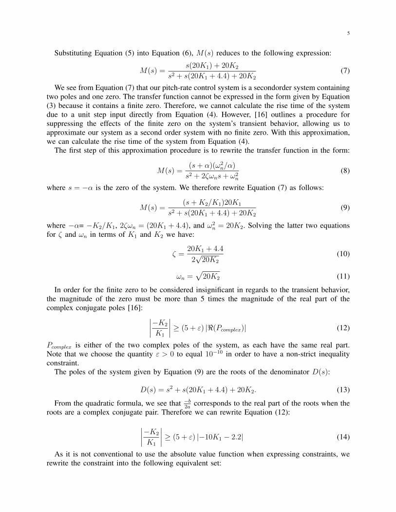
VI. CONCLUSIONS AND FUTURE WORK

The optimal K1 and K2 values which satisfy the constraints and give us the optimal rise timewere found to be K1 = 0.3667 and K2 = 10.7556, with an optimal rise time of tr = 0.1475s.We showed that the solution is insensitive to changes in constraints given by Equation (23d)and Equation (23e). We showed that the solution is sensitive to changes in constraints givenby Equation (23b), Equation (23c), and Equation (23f). This sensitivity was justified throughcontrol theory.

By using the dominant poles method to give a closed form solution of the rise time expression,we reduce the accuracy of the performance criterion. However, this is necessary, as the onlyother options either produce a lengthy (many page) expression for rise time, or give numericalapproximations for rise time. As it is required that we rigorously prove that a minimum existsfor the rise time objective function, such alternates are ruled out.

Initially, we attempted to formulate a general proof for showing the existence of a minimum.This method would not call for a closed form expression of rise time, and would use real analysisto show that the rise time function is guaranteed to be continuous [22]. From there, we wouldbe able to apply Weierstrass’ theorem to show that a minimum value exists. This would beespecially useful for higher order systems, as a closed form expression for rise time fails toexist past order two, unless the dominant pole method or other methods are applied to modelthe system as a second order.

The method involves showing that continuity is preserved through a series of steps. The firststep would be to show that the inverse Laplace transform of the step response, c(t), is continuous.Next, we show that the inverse function of the response, t(c), is continuous. Then, we show thatthe “first crossing function” (the time when the inverse function reaches a specified c(t)) of theinverse function at c(t) = 0.1 and c(t) = 0.9 is continuous. By subtracting these “first crossingfunctions”, we would have an expression for rise time. If the operations were shown to preservecontinuity, then the rise time function is shown to be continuous. This method is powerful inthat we do not necessarily need to evaluate all the expressions, but can still show that continuityis preserved. However, the mathematics proved way beyond our abilities, and such a methodwas abandoned.

This sidelined any attempt to move to a higher order representation of the system dynamics.We attempted to use fourth order system dynamics (fifth order closed loop transfer function) [8]but this proved too challenging. Use of even a second order representation of pitch rate dynamicsmakes it very difficult to keep our performance expressions in a closed form. Even by applyingthe dominant pole method to second order pitch rate dynamics (third order system) [12], wefound the percent overshoot is necessarily very large (over 80%). Therefore, in our paper weonly explore the problem with first order pitch rate dynamics.

A similar issue was encountered when expanding our work to include a derivative controller.This control element added an additional zero into our closed loop transfer function, which madeour previous rise time approximation infeasible. The only option in this case was the long andcalculation expensive method discussed earlier, which proved beyond our mathematical ability.

The necessity in proving rigorously that a minimum exists also impedes efforts to raise theorder of the pitch rate dynamics. In fact, it is almost definite that higher order systems cannotbe optimized with the requirement that existence of a minimum be proved.

With the current restrictions on the project, future work in optimizing rise time for pitch ratecontrol systems is very difficult. Even if the controls scheme is changed, the same issues wouldbe present, and the rise time expression would be very difficult to find. Future research into a

15

performance criterion that can be easily be expressed in a closed form would prove very usefulfor controls engineers.

16

REFERENCES

[1] K. Ogata, Modern Control Engineering. Englewood Cliffs, NJ: Prentice-Hall, 1970.[2] T. Benson. (2008) Aircraft rotations. [Online]. Available: http://www.grc.nasa.gov/WWW/k-12/airplane/rotations.html[3] D. McLean, “Globally stable nonlinear flight control system,” IEEE Proceedings Pt. D Control Theory and Applications,

vol. 130, no. 3, p. 93, May 1983.[4] D. Saussie et al., “Aircraft pitch rate control design with guardian maps,” in 18th Mediterranean Conf. Control Automation,

June 2010, pp. 1473 –1478.[5] S. Kamalasadan and A. Ghandakly, “Nonlinear fighter aircraft pitch-rate tracking using a multiple fuzzy reference model

adaptive controller,” in IEEE Int. Conf. Computational Intelligence for Measurement Systems and Applications, July 2005,pp. 44 – 49.

[6] S. Kamalasadan and A. Ghandakly, “A neural network parallel adaptive controller for fighter aircraft pitch-rate tracking,”IEEE Trans. Instrum. Meas., vol. 60, no. 1, pp. 258 –267, Jan. 2011.

[7] C. Hao et al., “Sliding mode controller design for an aircraft pitch rate track system,” in IEEE Int. Conf. on Networking,Sensing and Control, April 2008, pp. 1004 –1007.

[8] S. M. Shinners, Advanced Modern Control System Theory and Design. New York: Wiley, 1998.[9] F. Demourant et. al, “Falsification of an aircraft autopilot,” in American Control Conference, 2002. Proceedings of the

2002, vol. 1, 2002, pp. 803 – 808 vol.1.[10] L. Jinli and D. Manfeng, “Fuzzy adaptive pi control for near space aircraft electric propulsion system,” in Int. Conf.

Computer, Mechatronics, Control and Electronic Engineering, vol. 4, Aug. 2010, pp. 472 –475.[11] G. J. Balas et al., “Control of the f-14 aircraft lateral-direction axis during powered approach,” Journal of Guidance,

Control, and Dynamics, vol. 21, no. 6, pp. 258 –267, Nov. 1998.[12] C. Barbu et al., “Anti-windup design for manual flight control,” in Proc. American Control Conf., vol. 5, 1999, pp. 3186

–3190.[13] E. G. Rynaski, “The interpretation of flying qualities requirements for flight control system design,” unpublished.[14] J. W. Brown and R. V. Churchill, Complex Variables and Applications. New York: McGraw-Hill, 2009.[15] S. M. Shinners, Modern Control System Theory and Design. New York: Wiley, 1998.[16] M. Gopal, Control Systems Principles and Design. New Delhi, India: Tata McGraw Hill, 2002.[17] H. K. Ahmad, private communication, 2011.[18] E. K. Chong and S. H. Zak, An Introduction to Optimization. Hoboken, NJ: Wiley, 2008.[19] LOQO Users Manual, R. J. Vanderbei, 2006.[20] Product documentation: fmincon. [Online]. Available: http://www.mathworks.com/help/toolbox/optim/ug/fmincon.html[21] Product documentation: stepinfo. [Online]. Available: http://www.mathworks.com/help/toolbox/control/ref/stepinfo.html[22] S. M. Mintchev, private communication, 2011.

17

VII. MATLAB CODE

The following script runs the solution algorithm. We use the active set algorithm with the fminconsolver to find the optimal solution.

1 % Thi s s c r i p t r u n s t h e s o l u t i o n a l g o r i t h m . We use t h e a c t i v e s e t a l g o r i t h m2 % wi th t h e fmincon s o l v e r t o f i n d t h e o p t i m a l s o l u t i o n .34 c l e a r ; c l o s e a l l ; c l c ;5 k0 = [ 0 . 1 2 . 1 ] ; % s t a r t i n g g u e s s67 options = optimset ( ' A lgo r i t hm ' , ' a c t i v e−s e t ' ) ;8 [k ,fval ] = fmincon (@rise_time ,k0 , [ ] , [ ] , [ ] , [ ] , [ − 1 ] , [ 1 5 ] , @constraints ,options ) ;9

10 % P r i n t o p t i m a l k v a l u e s and r i s e t ime11 k12 rt = rise_time (k )1314 % P l o t s t e p r e s p o n s e15 den_a = 1 ;16 den_b = ( 2 0 . *k ( 1 ) + 4 . 4 ) ;17 den_c = 2 0 . *k ( 2 ) ;18 step (tf ( [ 2 0 *k ( 1 ) 20*k ( 2 ) ] , [den_a den_b den_c ] ) )

The following function gives rise time for an input K vector. This serves as our objectivefunction.

1 % F u n c t i o n t h a t g i v e s r i s e t ime f o r an i n p u t K v e c t o r . Th i s s e r v e s as our2 % o b j e c t i v e f u n c t i o n .34 f u n c t i o n f = rise_time (k )5 zeta = ( 2 0 . *k ( 1 ) + 4 . 4 ) . / ( 2 . * ( 2 0 . *k ( 2 ) ) . ˆ ( 1 / 2 ) ) ;6 w_n = (20*k ( 2 ) ) ˆ ( 1 / 2 ) ;7 f = ( p i − acos (zeta ) ) / ( (w_n ) * (1 − zeta ˆ 2 ) ˆ ( 1 / 2 ) ) ;

The following function serves to call our constraints for the fmincon solver.

1 % Thi s f u n c t i o n s e r v e s t o c a l l our c o n s t r a i n t s f o r t h e fmincon s o l v e r .23 f u n c t i o n [c ,ceq ] = constraints (k )45 % d e f i n i n g d e n o m i n a t o r o f t r a n s f e r f u n c t i o n ( c o e f f i c i e n t s o f p o l y n o m i a l )6 den_a = ones ( s i z e (k ( 1 ) ) ) ;7 den_b = ( 2 0 . *k ( 1 ) + 4 . 4 ) ;8 den_c = 2 0 . *k ( 2 ) ;9

10 % s t a b i l i t y c o n s t r a i n t s : by e n s u r i n g a l l p o l e s a r e t o t h e l e f t o f s igma =11 % −0.5 i n t h e s−p l a n e . t h e s e c o n s t r a i n t s were d e t e r m i n e d by a p p l i c a t i o n o f12 % t h e m o d i f i e d r o u t h−h u r w i t z c r i t e r i o n .1314 c1 = −3.4/20 − k ( 1 ) ;15 c2 = 1 0 . *k ( 1 ) − 2 0 . *k ( 2 ) + 1 . 9 5 ;1617 % z e r o s u p p r e s s i o n c o n s t r a i n t : t o s u p p r e s s t h e e f f e c t s o f t h e z e r o i n t h e n u m e r a t o r o f t h e ←↩

t r a n s f e r18 % f u n c t i o n . do ing so w i l l a l l o w us t o use t h e s t a n d a r d second o r d e r19 % e x p r e s s i o n s f o r r e s p o n s e c h a r a c t e r i s t i c s .2021 c3 = −abs (−k ( 2 ) . / k ( 1 ) ) + (5+ eps ) . * abs (−10.*k ( 1 ) − 2 . 2 ) ;2223 % c o n s t r a i n t on t h e damping r a t i o ( z e t a )2425 zeta = ( 2 0 . *k ( 1 ) + 4 . 4 ) . / ( 4 . * ( 5 . * k ( 2 ) ) . ˆ ( 1 / 2 ) ) ;26 c4 = ( 0 . 4 − zeta ) ;27 c5 = (zeta − 0 . 7 ) ;

18

2829 % c o n s t r a i n t v e c t o r i n form c <= 03031 c = [c1 ; c2 ; c3 ; c4 ; c5 ] ;3233 ceq = [ ] ;

The following script plots the feasible set to produce Figure 4. Note the commented code onthe bottom of the script, which creates Figure 5.

1 % Code t h a t p l o t s f e a s i b l e s e t f o r r i s e t ime o p t i m i z a t i o n problem f o r second o r d e r sys tem .23 c l e a r ; c l c ; c l o s e a l l ;45 % t e s t p o i n t s6 [k1 ,k2 ] = meshgr id ( −1 : . 0 1 : 1 5 ) ;78 % pre−a l l o c a t i n g memory9 c1 = z e r o s ( s i z e (k1 ) ) ;

10 c2 = z e r o s ( s i z e (k1 ) ) ;11 c3 = z e r o s ( s i z e (k1 ) ) ;12 c4 = z e r o s ( s i z e (k1 ) ) ;13 c4_a = z e r o s ( s i z e (k1 ) ) ;14 c4_b = z e r o s ( s i z e (k1 ) ) ;15 den_a = z e r o s ( s i z e (k1 ) ) ;16 den_b = z e r o s ( s i z e (k1 ) ) ;17 den_c = z e r o s ( s i z e (k1 ) ) ;18 zeta = z e r o s ( s i z e (k1 ) ) ;19202122 % d e f i n i n g d e n o m i n a t o r o f t r a n s f e r f u n c t i o n ( c o e f f i c i e n t s o f p o l y n o m i a l )23 den_a = ones ( s i z e (k1 ) ) ;24 den_b = ( 2 0 . *k1 + 4 . 4 ) ;25 den_c = 2 0 . *k2 ;26272829 % s t a b i l i t y c o n s t r a i n t s : e n s u r i n g a l l p o l e s a r e t o t h e l e f t o f s igma =30 % −0.5 i n t h e s−p l a n e . t h e s e c o n s t r a i n t s were d e t e r m i n e d by a p p l i c a t i o n o f31 % t h e m o d i f i e d r o u t h−h u r w i t z c r i t e r i o n .3233 c1 = (k1 >= −3.4 /20) ;34 c2 = (−10.*k1 + 2 0 . *k2 −1.95 >= 0) ;353637 % z e r o s u p p r e s s i o n c o n s t r a i n t : t o s u p p r e s s t h e e f f e c t s o f t h e z e r o i n t h e n u m e r a t o r o f t h e ←↩

t r a n s f e r38 % f u n c t i o n . do ing so w i l l a l l o w us t o use t h e s t a n d a r d second o r d e r39 % e x p r e s s i o n s f o r r e s p o n s e c h a r a c t e r i s t i c s .4041 c3 = ( abs (−k2 . / k1 ) >= (5+ eps ) . * abs (−10.*k1 − 2 . 2 ) ) ;4243 % c o n s t r a i n t on t h e damping r a t i o ( z e t a )4445 zeta = ( 2 0 . *k1 + 4 . 4 ) . / ( 4 . * ( 5 . * k2 ) . ˆ ( 1 / 2 ) ) ;46 c4_a = ( 0 . 4 <= zeta ) ;47 c4_b = (zeta <= 0 . 7 ) ;48 c4 = c4_a . *c4_b ;495051 % v e c t o r t h a t sums a l l s u c c e s s f u l c o n s t r a i n t s52 z = c1+c2+c3+c4 ;5354 % number o f f e a s i b l e p o i n t s : d i s p l a y e d on s c r e e n55 s i z e ( f i n d (z == 4) )565758 %% P l o t

19

5960 val = f i n d (z == 4) ;61 p l o t (k1 (val ) ,k2 (val ) , ' ks ' ) ;62 ho ld on ;6364 % below i s t h e p l o t o f t h e c u r v e used i n t h e c o n t i n u i t y p r o o f65 % x = [ − 1 : . 0 1 : 1 0 ] ;66 % y = ( 1 / 5 ) . * ( 2 5 . * x . ˆ 2 + 1 1 . * x + 1 . 2 1 ) ;67 % p l o t ( x , y ) ;