Optimization of Temporary Haul Road Design and Earthmoving Job Planning based on

Site Rough-grading Design

by

Chang Liu

A thesis submitted in partial fulfillment of the requirements for the degree of

Master of Science

in

Construction Engineering and Management

Department of Civil and Environmental Engineering

University of Alberta

© Chang Liu, 2014

ii

ABSTRACT

Site rough-grading operations are the preliminary work of the construction projects in remote

areas especially in Northern Alberta. Haulage cost typically accounts for around 30% of the total

cost of mass earthmoving projects. The temporary haul road network built in the earthmoving

field is one major factor influencing haulage cost and production efficiency, which remains an

empirical design problem at present. In order to convert it into an analytical problem, this study

firstly utilizes the Floyd-Warshall algorithm and linear programming model to formulate the

earthmoving planning based on a certain layout of temporary road network, shedding light on the

potential benefits of selecting routes and directions for handling earthmoving jobs. On the basis

of the optimization of earthmoving job planning, the optimization of layout of temporary road

network is further proposed by using multi-generation compete genetic algorithm. The

optimization approaches are explained in details through a practical application. Based on

analytical analysis and numerical applications, it is proved that the optimization approach can

reduce the total cost of the project and shortens its duration. In addition, simulation models are

used to prove the effectiveness and feasibility of optimization results. The study conducts

comprehensive and in-depth analyses to tackle the temporary haul road network design problem

in the context of earthworks planning, which can provide decision support in planning and

executing massive earthworks.

iii

PREFACE

This thesis is an original work by Chang Liu. No part of this thesis has been previously

published.

iv

ACKNOWLEDGEMENT

I sincerely thank Dr. Ming Lu, my supervisor and mentor. I am extremely grateful for his vision,

support, encouragement, and guidance for years during my study. His sound knowledge, deep

thinking, and academic rigor have led my way to the successful completion of my MSc program,

as well as motivated me to bring out myself.

Special thanks to Sam Johnson, Project Manager, Commercial / Civil, Alberta North, Graham

Management Services for sharing his vision and insight and providing case study support in the

present research. His continuous support and assistance helped me in collecting and sharing

project data, analyzing construction processes, and gaining insight into field operations, which

provided me a great opportunity to obtain experience and knowledge on earthworks design and

construction.

v

Table of Contents

1 Introduction .............................................................................................................................. 1

2 Literature Review..................................................................................................................... 6

2.1 Limitations in Previous Research and Practice .......................................................... 8

2.2 Overview of Present Research ................................................................................. 10

2.3 Differences from Previous Research........................................................................ 12

3 Optimizations Based on Temporary Haul Road Networks Design ........................................ 16

3.1 Proposed Methodology ............................................................................................ 16

3.2 Optimization of Earthmoving Job Planning ............................................................ 18

3.2.1 Gird Model ........................................................................................................ 18

3.2.2 Floyd-Warshall Algorithm ................................................................................ 21

3.2.3 Linear Programming Model .............................................................................. 25

3.2.4 Cost Evaluation ................................................................................................. 27

3.3 Layout Optimization of Temporary Haul Road Network ........................................ 30

3.3.1 Input Data.......................................................................................................... 32

3.3.2 0-1 Problem ....................................................................................................... 33

3.3.3 Optimization Algorithm (Genetic Algorithm) .................................................. 34

4 Case Study ............................................................................................................................. 39

4.1 Practical Application to Achieve Optimized Earthmoving Plan .............................. 39

4.1.1 Comparison between Layout Options ............................................................... 40

4.1.2 Effect of Grid Size Selection ............................................................................ 46

4.1.3 Summary ........................................................................................................... 48

4.2 Practical Application to Optimize Layout of Temporary Haul Road Network ........ 49

4.2.1 Overview of Earthmoving Project .................................................................... 49

4.2.2 Optimization of Temporary Road Network ...................................................... 50

4.2.3 Simulation with Earthmoving Plans ................................................................. 57

vi

4.2.4 Summary ........................................................................................................... 60

4.3 Validation of Layout Optimization Approach .......................................................... 61

4.4 Cost Saving of Optimization Method ...................................................................... 63

5 Conclusions and Further Research ......................................................................................... 64

5.1 Conclusions .............................................................................................................. 64

5.2 Limitations ............................................................................................................... 66

5.3 Future Research ....................................................................................................... 68

References ..................................................................................................................................... 70

APPENDIX A. Program for Optimized Earthmoving Plan .......................................................... 74

Achievement of Earthmoving Plan (Layout Option 3) ................................................... 76

APPENDIX B. Program for Optimization of Temporary Haul Road Network ............................ 78

MCGA Functions ............................................................................................................ 78

vii

LIST OF TABLES

Table 3.1 Variables for Road Sections ......................................................................................... 20

Table 3.2 Shortest Haul Time between Cells................................................................................ 24

Table 3.3 Optimized Earthmoving Plan ........................................................................................ 27

Table 3.4 Parameters of Multi-generation Compete Genetic Algorithm ...................................... 35

Table 4.1 Comparison between Haul Road Layout Options ........................................................ 42

Table 4.2 Optimized Earthmoving Job Plans based on Layout Option 1 ..................................... 43

Table 4.3 Optimized Earthmoving Job Plans based on Layout Option 3 ..................................... 44

Table 4.4 Comparison between Grid Sizes - Layout Option 1 ..................................................... 47

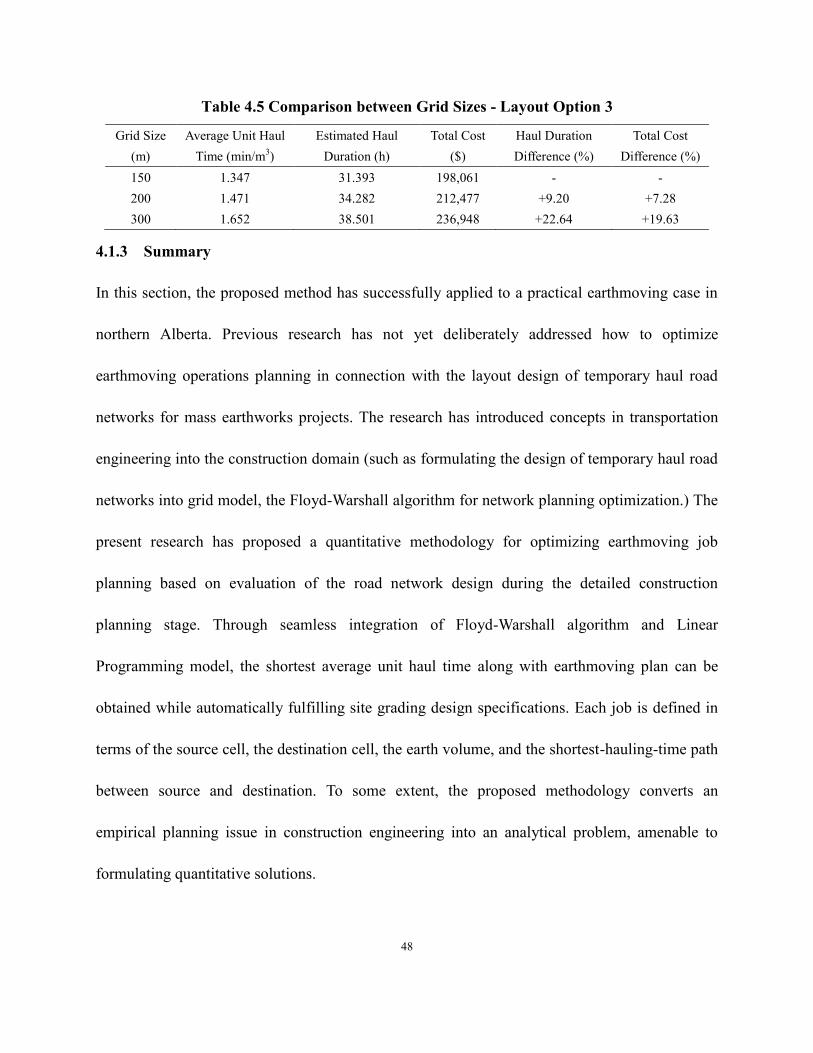
Table 4.5 Comparison between Grid Sizes - Layout Option 3 ..................................................... 48

Table 4.6 Comparison between Different Layouts ....................................................................... 53

Table 4.7 Optimized Earthmoving Plan based on the Optimal Layout ........................................ 54

Table 4.8 The Duration, Capacity and Resource of Tasks ........................................................... 59

Table 4.9 Comparison between Models........................................................................................ 62

viii

LIST OF FIGURES

Figure 1.1 Optimization Flowchart ................................................................................................. 4

Figure 2.1 AGTEK Interface .......................................................................................................... 6

Figure 3.1 Flowchart of the Methodology .................................................................................... 16

Figure 3.2 Distance between Two Accesses to Main Haul Road (D) .......................................... 19

Figure 3.3 Grid Model for Layout Design .................................................................................... 20

Figure 3.4 Earthmoving Volume of Cells (m3) ............................................................................. 26

Figure 3.5 Optimized Earthmoving Plan (m3) .............................................................................. 27

Figure 3.6 Flowchart of Layout Optimization .............................................................................. 31

Figure 3.7 Curved Alignment Represented by Diagonal Link ..................................................... 33

Figure 3.8 0-1 Model for Potential Temporary Road Networks ................................................... 34

Figure 3.9 Flowchart of Optimization Approach .......................................................................... 36

Figure 4.1 Volume of Cells based on Division of the Field (m3) ................................................. 39

Figure 4.2 Layout Option 1 ........................................................................................................... 41

Figure 4.3 Layout Option 2 ........................................................................................................... 41

Figure 4.4 Layout Option 3 ........................................................................................................... 41

Figure 4.5 Layout Option 4 ........................................................................................................... 41

Figure 4.6 Designed Cut and Fill Areas of Rough Grading Design ............................................. 50

Figure 4.7 Empirical Temporary Road Network .......................................................................... 50

Figure 4.8 Optimization of Temporary Road Network ................................................................ 51

Figure 4.9 Temporary Road Network Model based on Optimized Solutions .............................. 53

Figure 4.10 Simulation Model in Simphony Encoded with Earthmoving Plan ............................ 58

Figure 4.11 Code in the “Execution” Activity .............................................................................. 59

Figure 4.12 Cycle Time of Truck Loading ................................................................................... 60

ix

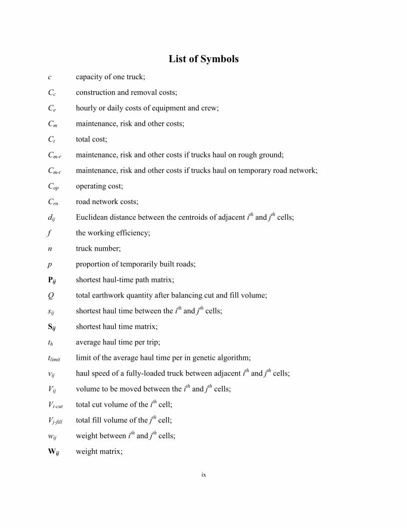
List of Symbols

c capacity of one truck;

Cc construction and removal costs;

Ce hourly or daily costs of equipment and crew;

Cm maintenance, risk and other costs;

Ct total cost;

Cm-r maintenance, risk and other costs if trucks haul on rough ground;

Cm-t maintenance, risk and other costs if trucks haul on temporary road network;

Cop operating cost;

Crn road network costs;

dij Euclidean distance between the centroids of adjacent ith

and jth

cells;

f the working efficiency;

n truck number;

p proportion of temporarily built roads;

Pij shortest haul-time path matrix;

Q total earthwork quantity after balancing cut and fill volume;

sij shortest haul time between the ith

and jth

cells;

Sij shortest haul time matrix;

th average haul time per trip;

tlimit limit of the average haul time per in genetic algorithm;

vij haul speed of a fully-loaded truck between adjacent ith

and jth

cells;

Vij volume to be moved between the ith

and jth

cells;

Vi-cut total cut volume of the ith

cell;

Vj-fill total fill volume of the jth

cell;

wij weight between ith

and jth

cells;

Wij weight matrix;

1

1 Introduction

The temporary road network design is a major factor influencing haulage cost and production

efficiency for mass earthworks in remote areas. So far the design of haul road network relies on

experience and there is no analytical method to achieve optimal layout. To increase the

earthmoving productivity and save cost, there is an immediate necessity to augment currently

empirical design methods with analytical methods.

In order to ensure safety and productivity of earthmoving operations in the preliminary

site-grading phase of developing infrastructure, mining and industrial projects, temporary haul

road networks are designed, developed, and maintained, which generally contain many

intersections and carry complicated traffic flows of heavy trucks. In current practice of mining

engineering, guidelines are generally available to regulate on all aspects of haul road design on

mining projects, including its alignment, surface, material and trucks operating on it so as to

ensure efficiency and safety; for instance, the road width should be 3 to 4 times the width of the

widest heavy hauler (Tannant and Regensburg 2001). Unlike the mining project, for site grading

and earthmoving operations over a large area, it is not realistic to link a loading area (cut) and a

dumpsite area (fill) by permanent haul roads. The common practice is to build a limited length of

temporary haul roads (e.g. gravel surfaced) along the critical truck hauling paths on site. Those

haul roads need to be maintained from time to time and eventually removed at the end of

2

construction. Trucks also need to operate on rough-ground roads, which require the frequent use

of graders or bulldozers to maintain serviceability.

As a critical component of planning mass earthworks projects, haul road network should be

well-planned and designed based on the available information such as site grading designs (cut

and fill design). As for haul road network layout design, there are two main tasks: 1) to design a

cost-efficient haul road network which is conducive to delivering the project within the expected

duration and budget; and 2) to achieve an execution earthmoving plan for the operators to

execute at the earthmoving stage. To achieve optimized earthmoving planning, the present

research connects the concepts in transportation engineering with construction engineering. To

further design an effective haul road network, the present research proposes a grid-based

temporary haul road network design and optimization method applicable to a site for which

grading design has been completed.

In Chapter 3, adding to the existing body of knowledge, a quantitative methodology for

optimizing the detailed planning of earthmoving jobs based on a particular temporary haul road

network design is proposed. Each job is defined in terms of the source cell, the destination cell,

the earth volume, and the shortest-hauling-time path between the source and destination.

Through seamless integration of the Floyd-Warshall algorithm and linear programming model,

following the existing haul road network, the shortest average unit haul time of trucks can be

3

obtained. Based on the resulting average unit haul time, cost equations are defined to account for

1) the direct truck-hauling crew cost and 2) building, maintenance and removal costs of

temporary haul roads. As such, the cost associated with executing the optimized earthmoving job

plan over a particular haul road network design can be readily assessed, making it

straightforward for project managers to evaluate the layout design.

Current empirical design methods cannot guarantee the generation of the most cost-effective

temporary haul road network design. Based on the evaluation criteria after establishing the

approach for achieving optimized earthmoving planning, different design layouts can be

compared with one another on the same basis, which provides the opportunity to optimize the

layout of temporary haul road network through heuristic searching algorithms. In Chapter 3, the

layout optimization method is also established on the basis of the Floyd-Warshall algorithm and

a linear programming model. Based on the genetic algorithm and the objective function defined

for genetic algorithm, the optimal layout design of temporary haul road network can be achieved

so that the decision-makers can finally benefit from an optimized layout in the planning stage.

The road planning problem is no longer empirical, and it becomes analytical and solvable as part

of earthworks design so to some extent the research successfully solves a subjective planning

problem in an objective fashion. The proposed approach could assist both experienced

decision-makers and junior engineers to identify an optimized temporary haul road network

design along with earthmoving operations planning.

4

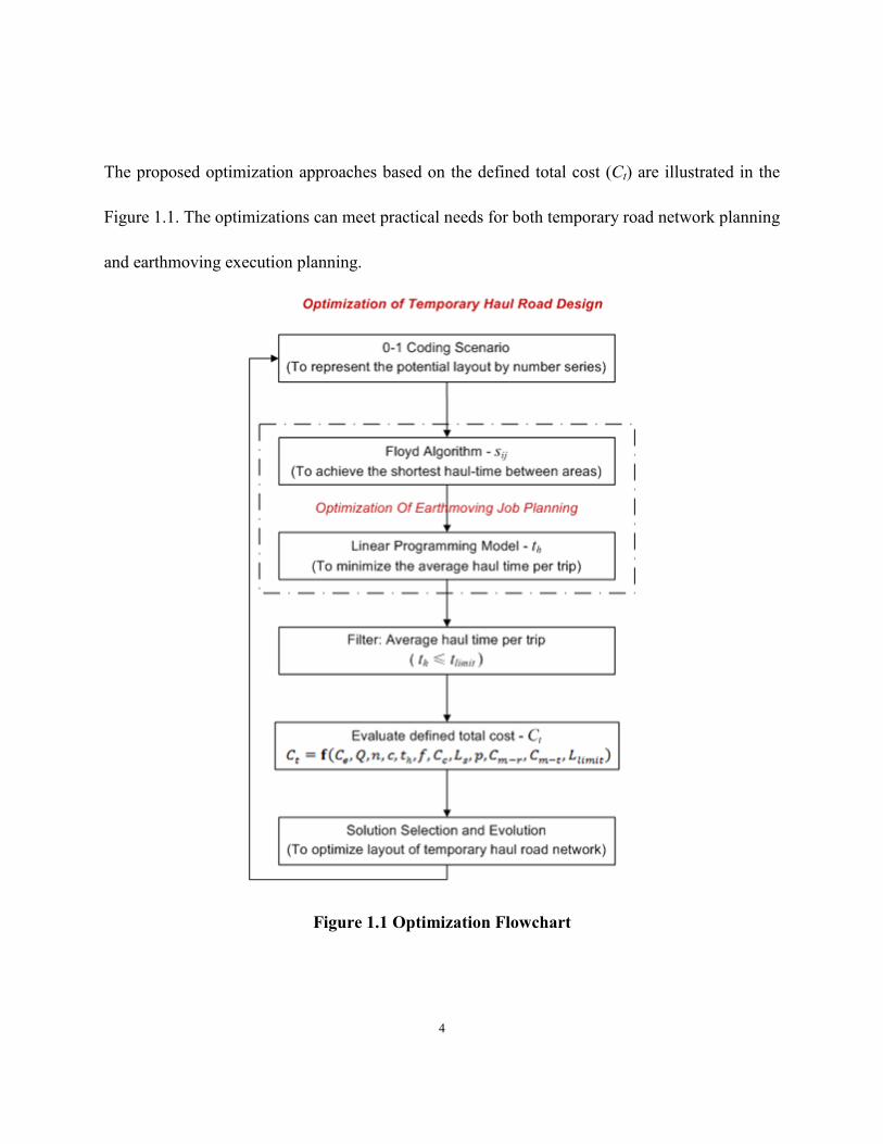
The proposed optimization approaches based on the defined total cost (Ct) are illustrated in the

Figure 1.1. The optimizations can meet practical needs for both temporary road network planning

and earthmoving execution planning.

Figure 1.1 Optimization Flowchart

5

The relationships between optimization of earthmoving job plan and optimization of temporary

haul road layout are demonstrated in the Figure 1.2. Although the optimization of earthmoving

job plan is embedded into the layout optimization at the planning stage, optimization of

earthmoving job plan can be performed separately based on the existing layout of haul road

network at the construction stage.

In Chapter 4, the proposed approaches are demonstrated in steps using numerical examples and

further applied in a case study which is a real-world massive earthmoving project in Northern

Alberta. Furthermore, simulation models are used as validation tool to prove the effectiveness

and feasibility of the optimization results. In addition, limitations of proposed methods and

conclusions are stated in Chapter 5.

6

2 Literature Review

Research has built a solid foundation for earthworks optimization, especially in regard to

balancing cut and fill volumes in site-grading design. Theoretically, it is widely held that project

cost can be minimized through formulating an optimal plan for transportation of materials

between cut sections and fill sections (Mayer and Stark 1981). Among the optimization

approaches, mass diagram is the simplest and the most commonly used especially for planning

linear construction projects such as road construction (Jayawardane and Harris 1990). To address

more complex problems, linear programming model plays the key role to minimize haul

distances and decide haul directions for earthmoving operations (Son et al. 2005). With the

ever-increasing computing power, large-scale optimizations for mass earthworks can be readily

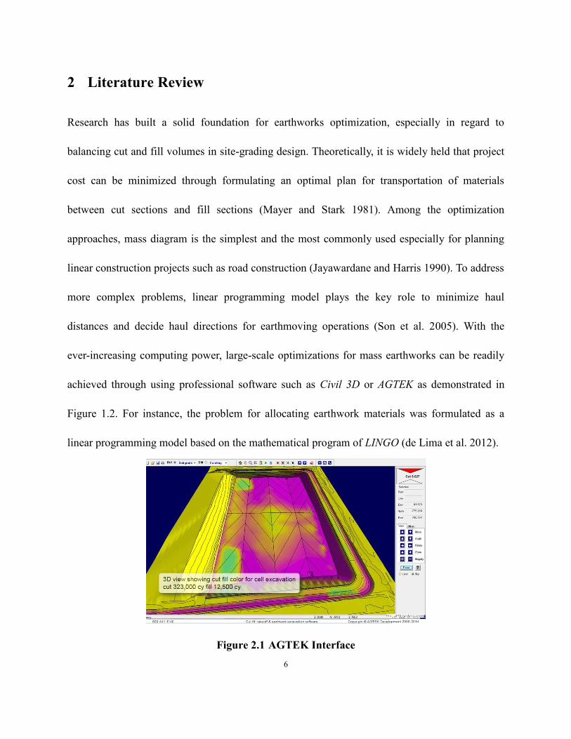
achieved through using professional software such as Civil 3D or AGTEK as demonstrated in

Figure 1.2. For instance, the problem for allocating earthwork materials was formulated as a

linear programming model based on the mathematical program of LINGO (de Lima et al. 2012).

Figure 2.1 AGTEK Interface

7

With the rapid development of computer technology, discrete event simulation has provided the

key methodology to lend effective, relevant decision support for productivity improvement on

earthworks projects. Discrete event simulation is a powerful tool to simulate earthmoving

operations by factoring in uncertainties. Simulation applications are mainly intended to guide

fleet selection and improve productivity of earthmoving operations. Resource-based earthmoving

simulation shows its great value in practical applications (Oloufa 1993; Shi and AbouRizk 1994;

Hajjar and AbouRizk 1997). With the introduction of evolutionary optimization algorithms,

earthwork simulation tools are further enhanced (Marzouk and Moselhi 2003). Integrating

pervious research, Moselhi and Alshibani (2009) developed the simulation model for large-scale

earthmoving operations. The researches provide insight for improving earthworks, but none has

yet formulated a quantitative approach to enhance the cost efficiency of hauling operations by

optimizing the design a haul road network. It is noteworthy that simulation research cannot help

to improve the layout of haul road network and therefore cannot help to establish the

fundamental theory for haul road network layout optimization.

The layout design of haul roads in earthworks can also be classified into “site layout planning

problem” in research. Site-layout plan optimization generally assumes the Euclidean distance

between two site locations as the travel distance by material handling resources (Zhang et al.

2008; Sanad et al. 2008; Said et al. 2013). It is noteworthy that Euclidean distances were also

applied in calculation of haul distances in earthworks design and planning (Son et al. 2005) and

8

average haul distance of trucks are essential criteria in real practice for decades, which can help

to estimate cycle time of trucks and direct cost.

2.1 Limitations in Previous Research and Practice

The temporary nature and the complexity inherent in designing an efficient haul road network

during the earthmoving operations planning stage have led to a lack of sophisticated guidelines

and a shortage of analytic techniques in the construction engineering and management domain.

Despite substantial advances, construction operations simulation and earthmoving optimization

research has not formalized methodologies that generate cost-effective plans for earthmoving

operations based on elaborate temporary haul road network design. This has partly accounted for

the fact that optimization results do not necessarily translate into efficiency and profitability in

practical applications.

Apparently, simulation models can provide practitioners with insight and lend them decision

support during the planning and execution stages of a construction project. On the other hand,

simulation models need to be built case by case, making a model specific to the input data

describing particular project scenarios and requiring significant efforts to update a model.

Additionally, in previous earthmoving simulation research, earthmoving jobs were assumed to be

well defined in terms of volume, source, and destination, while the research objectives were

largely to select the most efficient fleet and improve resource utilization by eliminating unwanted

9

waiting or queuing time. In general, earthmoving job planning integrated with the temporary

road network design has not yet been dealt with in an integrative fashion in previous simulation

research.

With regards to optimization research, research deliverables from the mathematical formulation

are generally given in the form of either a cut-and-fill-balanced earthworks design (Ji et al. 2009)

or minimized haul distances with haul directions for earthmoving operations (Son et al. 2005),

without factoring in the haul road network design. The conventional method is to represent the

haul distance by linking the centroid of a cut cell to that of a fill cell with a straight line section.

It should be pointed out, the Euclidean distance, which represents the point-to-point straight-line

path in a site layout model (as in Son et al. 2005), does not in general factor in a haul road

network on a construction site. This oversimplifies the haul road alignment design in practice

while also ignoring the cost and time implications of laying out temporary haul roads of different

grades (gravel road vs. rough ground) along different sections of the truck hauling path. As a

result, the haul distance estimate used in planning analyses can be significantly shorter than the

actual situation in the field; while given the same distance of a haul road section, the average

haul time of the truck can differ considerably when truck hauls on gravel surface instead of

rough ground.

Consequently, the research has not yet addressed the immediate needs of field personnel by

10

accounting for sufficient details on earthmoving job planning. As such, the cost efficiency gained

from optimization analysis cannot be clearly communicated and readily materialized in the field.

In order to overcome the identified limitations in previous simulation and optimization research,

the present research is intended to take an integrative approach to problem definition and

optimization formulation in such a way that the resulting haul road network layout design can be

passed to the superintendent in the field, along with the associated detailed earthmoving job plan.

2.2 Overview of Present Research

To address the “earthmoving job planning over haul road network” problem and assist in making

critical decisions in practice, this research is intended to add to the state of the art in construction

optimization and simulation by proposing a new methodology. The methodology optimizes the

planning of detailed earthmoving jobs based on a particular haul road network design, by

seamlessly integrating a linear programming model formulation and a shortest-path-finding

algorithm commonly applied in transportation engineering. As such, the objective of generating

earthmoving job plans and haul road network designs can be simultaneously fulfilled, achieving

both time-efficiency and cost-effectiveness.

In order for a contractor to justify the building and maintenance costs of temporary haul road

networks, project duration needs to be accelerated without significantly increasing the project

cost. In the present research, a cost function is defined to serve as an effective performance

11

measurement of the temporary haul road network design, which is based on 1) the average

hauling time per hauling trip resulting from the optimization analysis; and 2) the total length of

temporary haul road in the site. The cost function also accounts for direct truck-hauling crew

costs and indirect costs for constructing and maintaining temporary haul roads and rough-ground

roads. As such, the cost associated with executing the optimized earthmoving job plan over a

particular layout design of temporary haul road network can be readily estimated, making it

straightforward for project managers to compare alternatives and select the best one manual or

through heuristic searching algorithm.

In regards to earthmoving job planning optimization based on a detailed haul road network

design, the use of the haul time for a truck to move earth from the source location to the

destination location is a more appropriate performance measure than the haul distance due

mainly to two facts: 1) the turn-by-turn travel path on the haul road network needs to be

specified for each earthmoving job, while multiple path choices may exist between the same

origin and destination; 2) truck hauling speeds differ considerably on different types of roads in

the haul road network (temporary gravel-surfaced haul road vs. rough-ground road), while costs

to build and maintain various types of haul roads and rough-ground roads also markedly differ.

The remainder of this study starts with differentiating the long-haul vs. the short-haul problems

and two network optimization algorithms commonly applied in the transportation engineering

12

domain. Then, a grid-based temporary road network design method is introduced, applicable to a

typical site for which grading design and existing ground survey are completed. Further,

illustrated by a numerical case, mathematical formulations are provided for optimizing detailed

planning of earthmoving jobs based on a particular temporary haul road network design. Each

job is defined in terms of the source cell, the destination cell, the earth volume, and the

shortest-hauling-time path between source and destination cells. Next, a cost function is

established to ensure cost-effectiveness of the optimization results. To demonstrate the

application of the proposed methodology in a real-world setting, a case study is presented, in

which earthmoving plans based on alternative designs of temporary haul road networks are

generated and evaluated. Additionally, using the case study, the research also 1) validates the

haul road network design obtained from an independent optimization analysis by cross-checking

against the empirical design extracted based on the site layout of the actual case study; and 2)

sheds light on the effect of grid size selection upon sufficiency and accuracy of the proposed

grid-based methodology for haul road network design and earthmoving job plan. Conclusions are

drawn in the end in terms of academic and practical contributions of the present research along

with follow-up enhancements.

2.3 Differences from Previous Research

Short-Haul Problem vs. Long-haul Problem

Research has also addressed earthmoving operations in connection with planning long-distance

13

haul roads to export or import earth materials. A novel approach was developed for geography

information system (GIS)-based optimization of earthmoving site layout on a dam construction

project (Kang et al. 2013). The proposed approach was based on the Dijkstra’s algorithm, which

is essentially a shortest-path search algorithm in transportation engineering, mainly used for

route selection in tackling transportation and logistics problems. The same algorithm was also

used to optimize real-time operations of trucks in mining sites based on GPS, improving the

selection of routes (Choi and Nieto 2011).

It is noteworthy that for such long-haul problems, the cut and fill balance in the local site is

generally not an applicable constraint. A local site is commonly represented as one point on the

map associated with a particular quantity of earth to export or import. The site is connected to

nearby highways via access roads. As such, addressing long-haul problems is mainly concerned

with optimizing truck routing over a network of permanent roads and highways. In such cases,

the temporary haul road network design on a local site area is generally irrelevant. In contrast,

the problem of designing temporary haul road networks on an earthworks site can be treated as a

short-haul problem, which entails detailed analysis of earthmoving operations patterns between

multiple loading spots and multiple dumping spots.

The Floyd-Warshall algorithm is another classic algorithm for travel path optimization in the

transportation engineering domain. The Floyd-Warshall algorithm, originally developed by Floyd

14

(1962), has been used to solve a wide range of transport network planning and logistics planning

problems in transportation engineering (e.g. Pradhan and Mahinthakumar 2013; Dou et al. 2014).

Different from the Dijkstra’s Algorithm, the Floyd-Warshall algorithm is designed to handle a

large number of sources and thus provides an effective methodology to address the “earthmoving

job planning over haul road network” problem from the unique perspective of a

multi-source-multi-destination network planning problem in transportation engineering.

Rough-ground Road vs. Temporary Haul Road vs. Permanent Haul Road

In current practice of mining engineering, haul road design guidelines are already available to

regulate on all aspects of the haul road for mining projects, including its alignment, surface,

material and trucks operating on it so as to ensure efficiency and safety; for instance, the width of

haul road should be three to four times the width of the widest heavy hauler (Tannant and

Regensburg 2001). Unlike the mining project, for site grading and earthmoving operations over a

large area, it is not realistic to link a loading area (cut) and a dumpsite area (fill) by permanent or

semi-permanent haul roads since the project generally lasts several months. The common

practice is to build a limited length of temporary haul roads (e.g. gravel surfaced) along the

critical truck hauling paths on site. Those haul roads need to be maintained (e.g. watering) from

time to time and eventually removed at the end of construction. Haulers or trucks also need to

operate on original rough-ground of earthmoving field, which require the frequent use of graders

or bulldozers to maintain serviceability.

15

In the Guidelines for Mine Haul Road Design (Tannant and Regensburg 2001), haul roads are

categorized into temporary, semi-permanent and permanent haul road. The temporary road is

stated to be built with lower construction standards, which leads to higher rolling resistance. Due

to different needs in earthworks, transportation path with low traffic flow can be built with

low-standard temporary haul road or remain rough ground. Therefore, in a large-scale

earthmoving field, several different haul road sections comprise the temporary haul road network.

To quantitatively evaluate the cost-efficiency of certain layout of temporary haul road network, it

is meaningful to propose the analytical method and perform optimization. The decision makers

and project managers can benefit much through this study in earthworks.

16

3 Optimizations Based on Temporary Haul Road Networks Design

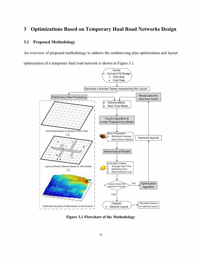
3.1 Proposed Methodology

An overview of proposed methodology to address the earthmoving plan optimization and layout

optimization of a temporary haul road network is shown in Figure 3.1.

Figure 3.1 Flowchart of the Methodology

17

The site grading design provides the main input and the site is divided into grids, with cell width

being 150 meters or 200 meters. Each line section linking the centroids of two adjacent cells in

the grid system horizontally, vertically, or diagonally is encoded as either 1 or 0, with “1” and “0”

denoting “gravel-surfaced haul road” and “rough-ground road”, respectively. Note allowing for

diagonally linking the centroids of two adjacent cells can effectively simplify any curved

alignment in haul road design. As such, a number series can be used to sufficiently represent a

potential layout design. Given the site grading design and the layout of the haul road network,

the earthwork volume matrix and the truck haul time matrix can be established. Then the

Floyd-Warshall algorithm and linear programming model are used to generate detailed

earthmoving job plans and identify particular truck-hauling paths for each earthmoving job. At

the end, the resulting earthmoving job plan is associated with the minimized average haul time

per trip based on a particular design. On the same basis, different alternatives of haul road

network designs for the same site can be analyzed and compared based on evaluation criteria

including average haul time, operating cost and road network cost. Thus the layout of temporary

road network can be improved gradually through heuristic searching algorithm and the optimal

layout can be finally achieved. In the following sections, important steps of the proposed

methodology are explained in details and illustrated by a numerical example.

18

3.2 Optimization of Earthmoving Job Planning

3.2.1 Gird Model

The grid model is applied to represent the potential layout of a temporary haul road network. It is

obvious that the grid size of a grid model is crucial to design the expected layout of road network.

Ideally, in order to increase the accuracy of earthworks quantity takeoff and haul time estimate,

the grid size should be as small as possible. Nonetheless, if grid size is so small that the field is

divided into a large number of cells, the road network design based on the grid system tends to

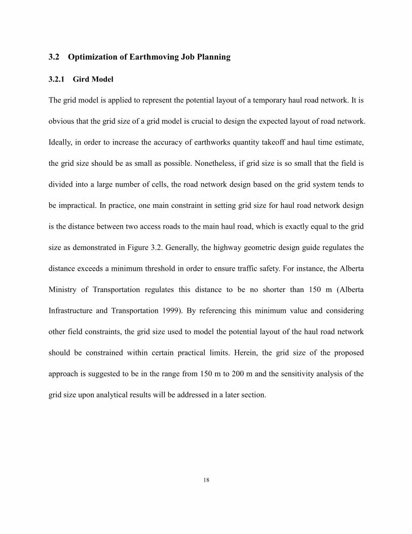
be impractical. In practice, one main constraint in setting grid size for haul road network design

is the distance between two access roads to the main haul road, which is exactly equal to the grid

size as demonstrated in Figure 3.2. Generally, the highway geometric design guide regulates the

distance exceeds a minimum threshold in order to ensure traffic safety. For instance, the Alberta

Ministry of Transportation regulates this distance to be no shorter than 150 m (Alberta

Infrastructure and Transportation 1999). By referencing this minimum value and considering

other field constraints, the grid size used to model the potential layout of the haul road network

should be constrained within certain practical limits. Herein, the grid size of the proposed

approach is suggested to be in the range from 150 m to 200 m and the sensitivity analysis of the

grid size upon analytical results will be addressed in a later section.

19

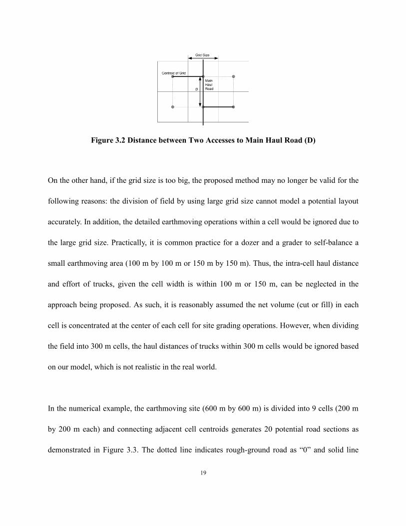
Figure 3.2 Distance between Two Accesses to Main Haul Road (D)

On the other hand, if the grid size is too big, the proposed method may no longer be valid for the

following reasons: the division of field by using large grid size cannot model a potential layout

accurately. In addition, the detailed earthmoving operations within a cell would be ignored due to

the large grid size. Practically, it is common practice for a dozer and a grader to self-balance a

small earthmoving area (100 m by 100 m or 150 m by 150 m). Thus, the intra-cell haul distance

and effort of trucks, given the cell width is within 100 m or 150 m, can be neglected in the

approach being proposed. As such, it is reasonably assumed the net volume (cut or fill) in each

cell is concentrated at the center of each cell for site grading operations. However, when dividing

the field into 300 m cells, the haul distances of trucks within 300 m cells would be ignored based

on our model, which is not realistic in the real world.

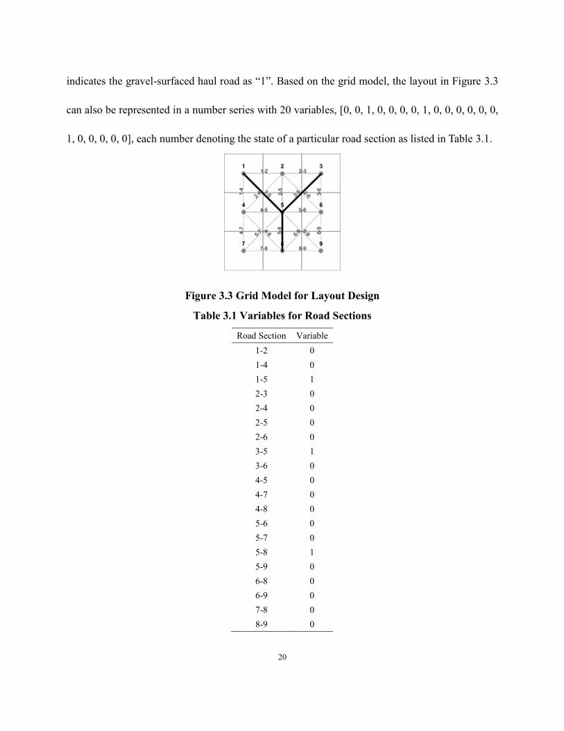
In the numerical example, the earthmoving site (600 m by 600 m) is divided into 9 cells (200 m

by 200 m each) and connecting adjacent cell centroids generates 20 potential road sections as

demonstrated in Figure 3.3. The dotted line indicates rough-ground road as “0” and solid line

20

indicates the gravel-surfaced haul road as “1”. Based on the grid model, the layout in Figure 3.3

can also be represented in a number series with 20 variables, [0, 0, 1, 0, 0, 0, 0, 1, 0, 0, 0, 0, 0, 0,

1, 0, 0, 0, 0, 0], each number denoting the state of a particular road section as listed in Table 3.1.

Figure 3.3 Grid Model for Layout Design

Table 3.1 Variables for Road Sections

Road Section Variable

1-2 0

1-4 0

1-5 1

2-3 0

2-4 0

2-5 0

2-6 0

3-5 1

3-6 0

4-5 0

4-7 0

4-8 0

5-6 0

5-7 0

5-8 1

5-9 0

6-8 0

6-9 0

7-8 0

8-9 0

21

3.2.2 Floyd-Warshall Algorithm

In the present research, the Floyd-Warshall algorithm is applied to identify the shortest-haul-time

path between a cut cell and a fill cell in the field, providing the crucial input in order to formulate

the optimal plan of earthmoving operations based on a haul road network design.

The optimization objective is to minimize the average haul time per trip while also identifying

the shortest origin-to-destination paths to move earth in the site. To identify the shortest path

between each pair of areas, all the combinations are enumerated and the solution is incrementally

improved until the solution reaches the minimum. The weight - which is assigned for each road

section connecting two adjacent cell centroids in the field grid - represents the haul time on the

corresponding road section. The weight matrix is calculated simply following the Eq. (1),

(1)

where wij is the weight between ith

and jth

cells, dij is the distance between centroids of adjacent

cells i and j and vij is the haul speed of a fully-loaded truck between adjacent cells i and j, which

is a variable depending on types of roads (gravel-surfaced haul road vs. rough-ground road).

In the numerical example, the haul speed of fully-loaded trucks on temporarily built

gravel-surfaced road and rough-ground road is assumed to be 27 km/h and 18 km/h, respectively.

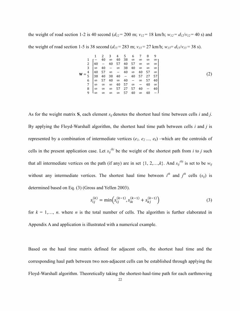
Given haul speeds and distances between cell centroids, the weight matrix W in terms of truck

hauling times can be determined by Eq. (2), where “∞” means no direct connection. For example,

22

the weight of road section 1-2 is 40 second (d12 = 200 m; v12 = 18 km/h; w12 = d12/v12 = 40 s) and

the weight of road section 1-5 is 38 second (d15 = 283 m; v15 = 27 km/h; w15= d15/v15 = 38 s).

[

]

(2)

As for the weight matrix S, each element sij denotes the shortest haul time between cells i and j.

By applying the Floyd-Warshall algorithm, the shortest haul time path between cells i and j is

represented by a combination of intermediate vertices (e1, e2 …, ek) –which are the centroids of

cells in the present application case. Let sij(k)

be the weight of the shortest path from i to j such

that all intermediate vertices on the path (if any) are in set {1, 2,…,k}. And sij(0)

is set to be wij

without any intermediate vertices. The shortest haul time between ith

and jth

cells (sij) is

determined based on Eq. (3) (Gross and Yellen 2003).

𝑠𝑖𝑗(𝑘) min(𝑠𝑖𝑗

(𝑘−1), 𝑠𝑖𝑘(𝑘−1) + 𝑠𝑘𝑗

(𝑘−1)) (3)

for k = 1,…, n. where n is the total number of cells. The algorithm is further elaborated in

Appendix A and application is illustrated with a numerical example.

Based on the haul time matrix defined for adjacent cells, the shortest haul time and the

corresponding haul path between two non-adjacent cells can be established through applying the

Floyd-Warshall algorithm. Theoretically taking the shortest-haul-time path for each earthmoving

23

job leads to the most time-efficient earthmoving operations on the road network.

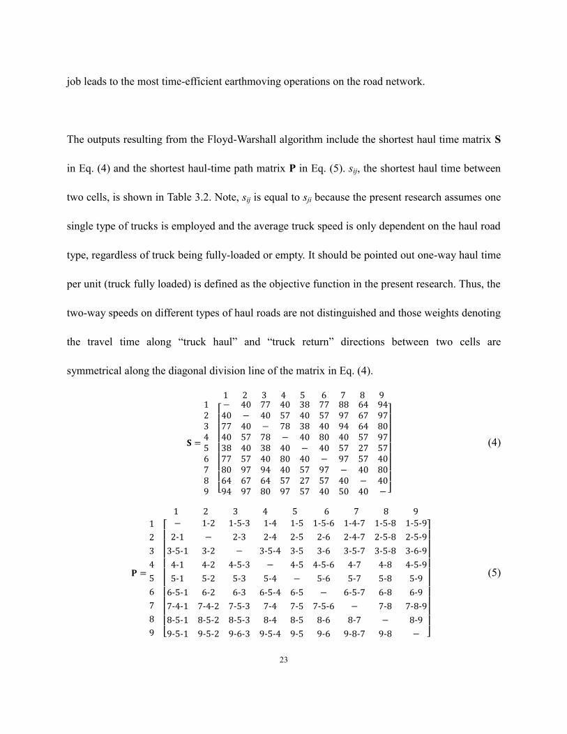
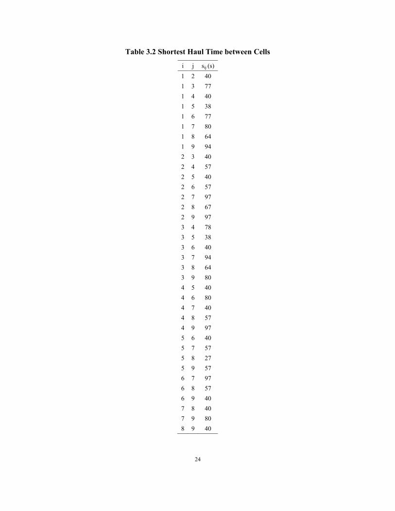
The outputs resulting from the Floyd-Warshall algorithm include the shortest haul time matrix S

in Eq. (4) and the shortest haul-time path matrix P in Eq. (5). sij, the shortest haul time between

two cells, is shown in Table 3.2. Note, sij is equal to sji because the present research assumes one

single type of trucks is employed and the average truck speed is only dependent on the haul road

type, regardless of truck being fully-loaded or empty. It should be pointed out one-way haul time

per unit (truck fully loaded) is defined as the objective function in the present research. Thus, the

two-way speeds on different types of haul roads are not distinguished and those weights denoting

the travel time along “truck haul” and “truck return” directions between two cells are

symmetrical along the diagonal division line of the matrix in Eq. (4).

𝐒

[

]

(4)

𝐏

[ - - - - - - - - - - - - -

- - - - - - - - - - -

- - - - - - - - - - - - -

- - - - - - - - - - -

- - - - - - - -

- - - - - - - - - - -

- - - - - - - - - - - - -

- - - - - - - - - - -

- - - - - - - - - - - - - ]

(5)

24

Table 3.2 Shortest Haul Time between Cells

i j sij (s)

1 2 40

1 3 77

1 4 40

1 5 38

1 6 77

1 7 80

1 8 64

1 9 94

2 3 40

2 4 57

2 5 40

2 6 57

2 7 97

2 8 67

2 9 97

3 4 78

3 5 38

3 6 40

3 7 94

3 8 64

3 9 80

4 5 40

4 6 80

4 7 40

4 8 57

4 9 97

5 6 40

5 7 57

5 8 27

5 9 57

6 7 97

6 8 57

6 9 40

7 8 40

7 9 80

8 9 40

25

3.2.3 Linear Programming Model

In addition to the shortest-haul-time path in the temporary haul road network, the optimal

earthmoving plan in terms of the volume, the source, and the destination of each job can be

generated at an upper level optimization formulation. As input data, the linear programming

model formulation requires the total cell volume matrix based on site grading design and the haul

time matrix resulting from the Floyd-Warshall algorithm. The total cut or fill volume of each cell

in the site grid system can be easily determined through gird-based quantity takeoff functions

available in current professional grading design and quantity takeoff software such as Civil 3D.

The resulting volume matrix serves as the boundary constraints in linear programming in terms

of the total cut or fill volume for each cell. Because the shortest haul time matrix is already

determined through Floyd-Warshall algorithm, the linear programming model demonstrated in

Eq. (6) can be used to generate detailed earthmoving jobs, achieving the minimized average

truck haul time per trip, given a certain temporary haul road network.

Min 𝑡ℎ ∑ ∑ 𝑠𝑖𝑗

𝑚𝑗=1

𝑛𝑖=1 𝑉𝑖𝑗

∑ ∑ 𝑉𝑖𝑗𝑚𝑗=1

𝑛𝑖=1

𝑠. 𝑡. ∑ 𝑉𝑖𝑗𝑚𝑗=1 𝑉𝑖−𝑐𝑢𝑡 , ≤ ≤ 𝑛

∑ 𝑉𝑖𝑗𝑛𝑖=1 𝑉𝑗−𝑓𝑖𝑙𝑙 , ≤ ≤ 𝑚

𝑉𝑖𝑗 ≥ , 𝑠𝑖𝑗 ≥

(6)

where th is the average haul time per trip, Vij is the volume to be moved between the ith

and jth

cells, Vi-cut is the total cut volume of the ith

cell, Vj-fill is the total fill volume of the jth

cell, and sij

is the shortest haul time between the ith

and jth

cells determined through applying the

Floyd-Warshall algorithm based on truck haul time between adjacent areas in the site.

26

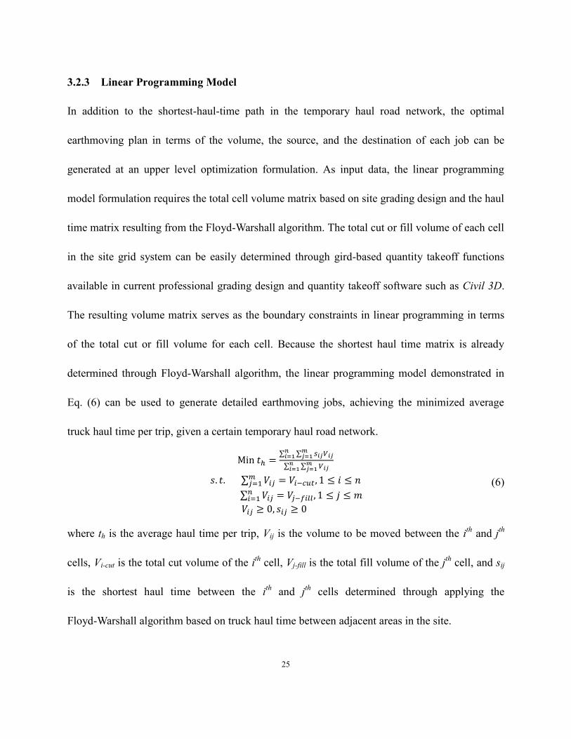
In the numerical example, the inputs of linear programming model include (1) the coefficients sij

in the shortest haul time matrix Sij and (2) the cell volumes, as shown in Figure 3.4. Note, the

number given in each cell represents its total volume of earthworks, with the minus sign “-”

denoting cut volume and the plus sign “+” denoting fill volume. Outputs of linear programming

model define specific earthmoving jobs, each being described by a specific source (cut cell), a

specific destination (fill cell), and a specific volume, along with a specific path. They can be

grouped together as the optimized earthmoving plan leading to the minimized average haul time

per trip.

Figure 3.4 Earthmoving Volume of Cells (m3)

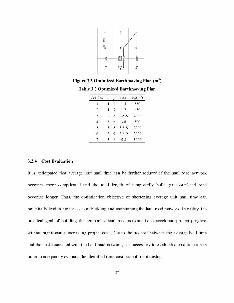
The proposed methodology, which is based on the integration of the Floyd-Warshall algorithm

and linear programming model, was coded into computer programs in Matlab in order to arrive

at the solutions. For the current case, the minimized average haul time is 52 s/m3 and the

earthmoving plan consisting of 7 jobs is demonstrated in Figure 3.5 and Table 3.3 ready for

execution at the construction stage.

27

Figure 3.5 Optimized Earthmoving Plan (m3)

Table 3.3 Optimized Earthmoving Plan

Job No. i j Path Vij (m3)

1 1 4 1-4 550

2 1 7 1-7 450

3 2 8 2-5-8 4000

4 3 6 3-6 800

5 3 8 3-5-8 2200

6 3 9 3-6-9 2000

7 5 8 5-8 5000

3.2.4 Cost Evaluation

It is anticipated that average unit haul time can be further reduced if the haul road network

becomes more complicated and the total length of temporarily built gravel-surfaced road

becomes longer. Thus, the optimization objective of shortening average unit haul time can

potentially lead to higher costs of building and maintaining the haul road network. In reality, the

practical goal of building the temporary haul road network is to accelerate project progress

without significantly increasing project cost. Due to the tradeoff between the average haul time

and the cost associated with the haul road network, it is necessary to establish a cost function in

order to adequately evaluate the identified time-cost tradeoff relationship.

28

The cost function should account for 1) direct truck hauling costs depending on the average unit

haul time and 2) costs relevant to building and maintaining temporary road networks, as in Eq.

(7). The direct truck-hauling cost (Cth) is given in Eq. (8) as the product of the hourly fleet cost

and total haul duration. The haul road network cost defined as Eq. (9) includes costs to build

gravel-surfaced haul roads and maintain both gravel surfaced and rough-ground haul roads.

𝐶𝑡 𝐶𝑡ℎ + 𝐶𝑟𝑛 (7)

𝐶𝑡ℎ 𝐶𝑒 ∙ 𝑇 (8)

𝐶𝑟𝑛 𝐶𝑐 + 𝐶𝑚 (9)

where Ct is the total cost, Cth is the direct truck-hauling cost, Crn is the road network related cost,

Ce is the hourly or daily cost of fleet equipment and crew, T is the total haul duration, Cc is the

construction and removal costs of the temporary haul road network related to lengths of roads of

various types, Cm is the maintenance, risk and other costs.

The total haul duration is estimated by Eq. (10),

𝑇 𝑄 (𝑛 ∙ 𝑐) ∙ 𝑡ℎ 𝑓 (10)

where Q is the total earthwork quantity in cubic meters (i.e. the total cut volume, which is equal

to the total fill volume for a cut-fill balanced grading site), n is the truck number (assuming the

use of a fleet of the same type of trucks), c is the volume capacity of one truck in cubic meters, th

is the average haul time which is actually the result of the above optimization analysis, and f is

29

the operations efficiency factor (45-min hour is generally applied in construction planning).

Due to the temporary nature of developing haul road networks on a mass earthworks project, the

maintenance cost of haul road can be simplified to be a function of the proportion of the length

of temporarily built gravel-surfaced haul roads over the total length of haul roads (including

rough-ground roads and gravel-surfaced haul roads). It is noteworthy that road maintenance costs

and vehicle operation/maintenance costs on rough ground roads and gravel-surfaced haul roads

differ substantially. Despite lower building cost, rough ground road is much more costly

considering such factors as frequent road maintenance, safety-related risks and more wear and

tear on tires and trucks.

Thus, the maintenance, risks and other cost as given in Eq. (11) is defined to account for the

effect of the proportion of temporarily built gravel-surfaced haul roads within the overall haul

road network on site.

𝐶𝑚 𝑝 ∙ 𝐶𝑚−𝑡 + ( 𝑝) ∙ 𝐶𝑚−𝑟 (11)

Where Cm-r is the maintenance, risk and other costs if trucks haul on rough-ground roads, Cm-t is

the maintenance, risk and other costs if trucks haul on gravel-surfaced haul roads, and p is the

proportion of temporarily built haul roads within the overall haul road network, which is the ratio

of the gravel-surfaced road length over the maximum road length in the current haul road

network design.

30

If there is no temporary gravel-surfaced haul road to be build, then p is 0%, and Cm will be

identical to the maintenance cost in connection with rough-ground roads Cm-r (Cm = Cm-r +

0%·Cm-t - 0%·Cm-r = Cm-r ). If trucks haul on gravel-surfaced haul roads across the entire site,

then p is 100%, and Cm will be equal to the maintenance cost in connection with temporarily

built haul roads Cm-t (Cm = Cm-r + 100 %·Cm-t - 100%·Cm-r = Cm-t ). Note comparing unit rates

($/km), Cm-r is generally much higher than Cm-t.

In order to ensure the cost-effectiveness of the road network design and the time-efficiency of the

derived earthmoving job plan, the cost of executing the optimized earthmoving job plan over a

particular road network design can be readily estimated by the established cost Eq. (7) to (9),

which will be demonstrated in the ensuing practical case study. This makes it straightforward for

project managers to compare multiple alternative designs and select the best one.

3.3 Layout Optimization of Temporary Haul Road Network

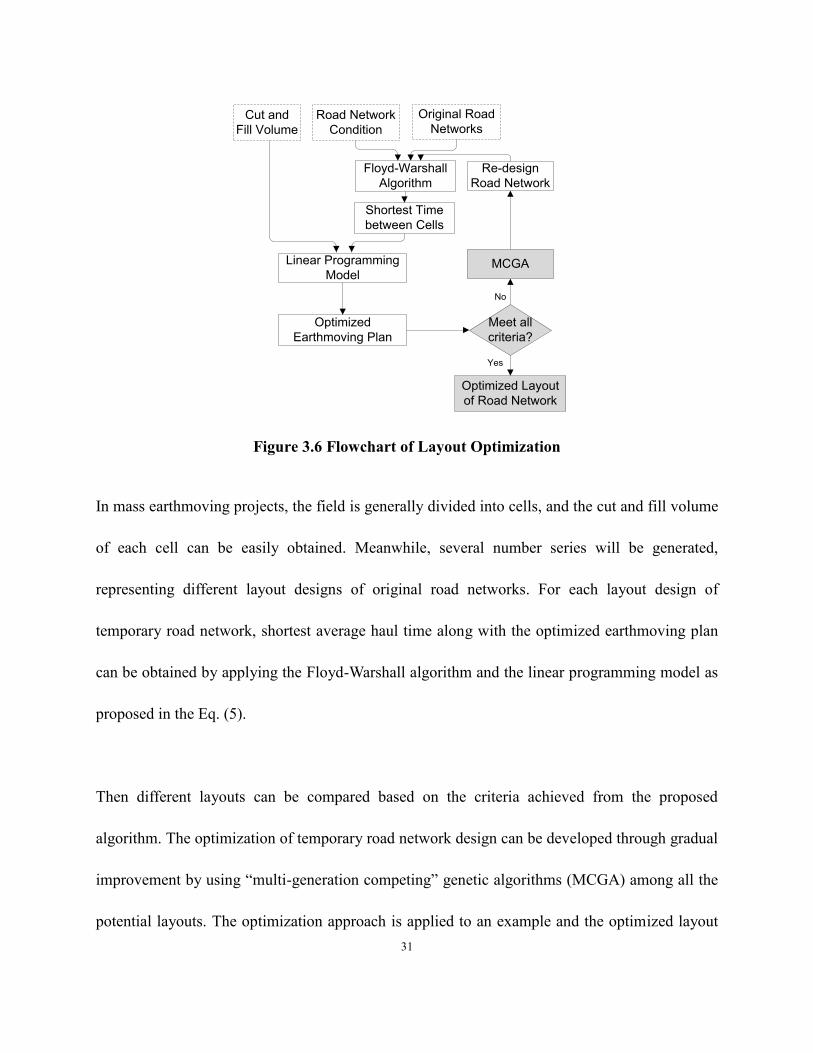
Based on Figure 3.1, Figure 3.6 further illustrates the details of proposed optimization approach

to achieve the optimized layout of temporary haul road network.

31

Cut and

Fill Volume

Road Network

Condition

Shortest Time

between Cells

Optimized

Earthmoving Plan

Re-design

Road Network

Original Road

Networks

Linear Programming

Model

Floyd-Warshall

Algorithm

MCGA

Optimized Layout

of Road Network

Meet all

criteria?

No

Yes

Figure 3.6 Flowchart of Layout Optimization

In mass earthmoving projects, the field is generally divided into cells, and the cut and fill volume

of each cell can be easily obtained. Meanwhile, several number series will be generated,

representing different layout designs of original road networks. For each layout design of

temporary road network, shortest average haul time along with the optimized earthmoving plan

can be obtained by applying the Floyd-Warshall algorithm and the linear programming model as

proposed in the Eq. (5).

Then different layouts can be compared based on the criteria achieved from the proposed

algorithm. The optimization of temporary road network design can be developed through gradual

improvement by using “multi-generation competing” genetic algorithms (MCGA) among all the

potential layouts. The optimization approach is applied to an example and the optimized layout

32

of temporary haul road network is eventually achieved. Simulation models encoded with

earthmoving plans are established in order to validate the optimization approach.

3.3.1 Input Data

According to the outline of earthmoving site, the field will be divided into cells, the cut and fill

volumes of cells is essential. Also, empirical or historical speed data of trucks is fundamental to

achieve optimized earthmoving plan. Therefore, to further achieve the optimized layout, the

inputs of proposed methodology include cut and fill data of the area (designed surface and raw

survey data preferred), different haul speeds of trucks on different surfaces, parameters of the

optimization algorithm and empirical or historical cost data as following:

Construction and removal costs of the gravel-surfaced temporary haul road;

Maintenance and other costs for the gravel-surfaced temporary haul roads and for rough

ground road respectively;

The maximum potential road length within the entire site area;

Mean truck-haul speed on temporary haul road;

Mean haul speed on rough ground;

Truck volume capacity;

Truck number;

Hourly cost of equipment and crew;

Working efficiency factor;

33

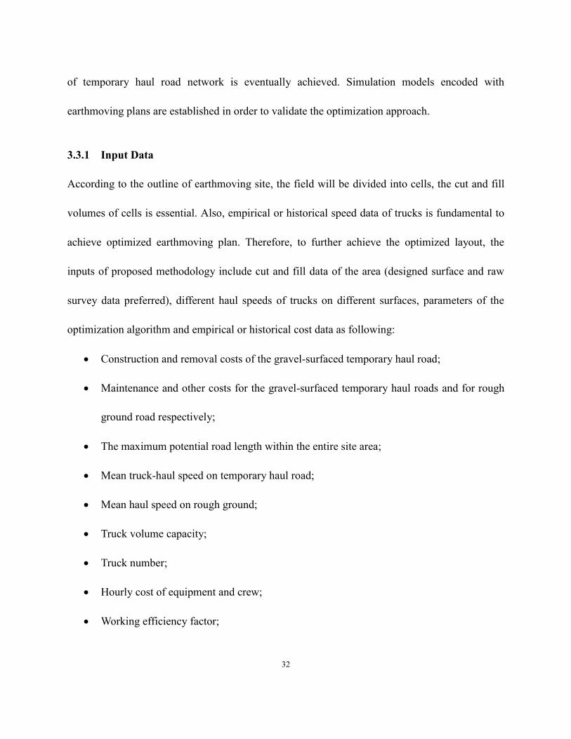
3.3.2 0-1 Problem

In this study, the haul road network layout design is based on a rectangular grid system with a

larger width that is applied to profile the site geometrically. The haul road alignment design is

constrained by the granularity of the grid system. Also, the curved alignment can be

approximated with by linking the centroids of two adjacent cells diagonally as demonstrated in

the Figure 3.7.

(a) Curved alignment (b) Road Network Model

Figure 3.7 Curved Alignment Represented by Diagonal Link

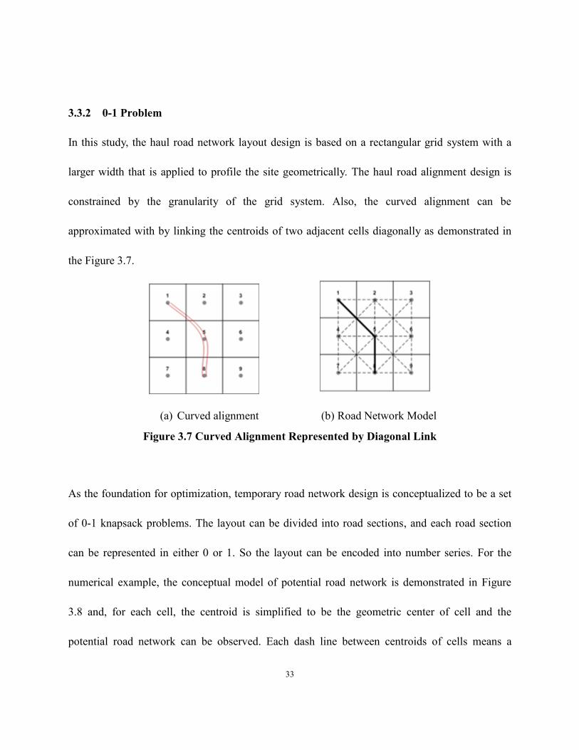
As the foundation for optimization, temporary road network design is conceptualized to be a set

of 0-1 knapsack problems. The layout can be divided into road sections, and each road section

can be represented in either 0 or 1. So the layout can be encoded into number series. For the

numerical example, the conceptual model of potential road network is demonstrated in Figure

3.8 and, for each cell, the centroid is simplified to be the geometric center of cell and the

potential road network can be observed. Each dash line between centroids of cells means a

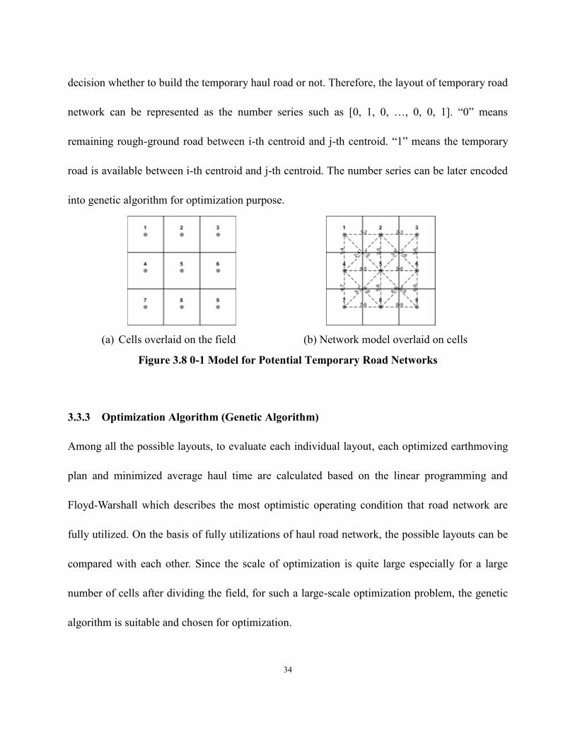
34

decision whether to build the temporary haul road or not. Therefore, the layout of temporary road

network can be represented as the number series such as [0, 1, 0, …, 0, 0, 1]. “0” means

remaining rough-ground road between i-th centroid and j-th centroid. “1” means the temporary

road is available between i-th centroid and j-th centroid. The number series can be later encoded

into genetic algorithm for optimization purpose.

(a) Cells overlaid on the field (b) Network model overlaid on cells

Figure 3.8 0-1 Model for Potential Temporary Road Networks

3.3.3 Optimization Algorithm (Genetic Algorithm)

Among all the possible layouts, to evaluate each individual layout, each optimized earthmoving

plan and minimized average haul time are calculated based on the linear programming and

Floyd-Warshall which describes the most optimistic operating condition that road network are

fully utilized. On the basis of fully utilizations of haul road network, the possible layouts can be

compared with each other. Since the scale of optimization is quite large especially for a large

number of cells after dividing the field, for such a large-scale optimization problem, the genetic

algorithm is suitable and chosen for optimization.

35

The optimization is accomplished through applying genetic algorithms to search the optimum

temporary road network design. Genetic algorithms have the limitation that it converges

towards a local optimum instead of the global optimum of the problem. MCGA, can address this

limitation to some extent and it confers the advantages including faster searching speed and

easier to achieve the global optimum (MCGA, Deng et al. 2007). Due to the significant

difference of computing time, multi-generation compete genetic algorithm is chosen and

programmed in MATLAB. The parameters of MCGA are given in the Table 3.4. The

Floyd-Warshall algorithm and linear programming model are embedded as the first two

consecutive analytical steps, which provide input to the GA optimization (referring to Fig. 3.9.).

Table 3.4 Parameters of Multi-generation Compete Genetic Algorithm

Variable Description

N Size of chromosomes depending on the temporary road network size;

MP Size of multi-generation;

NIND Number of individuals;

GGAP Generation gap;

MAXGEN Termination criteria which means the length of time during which minimum

value remains the same;

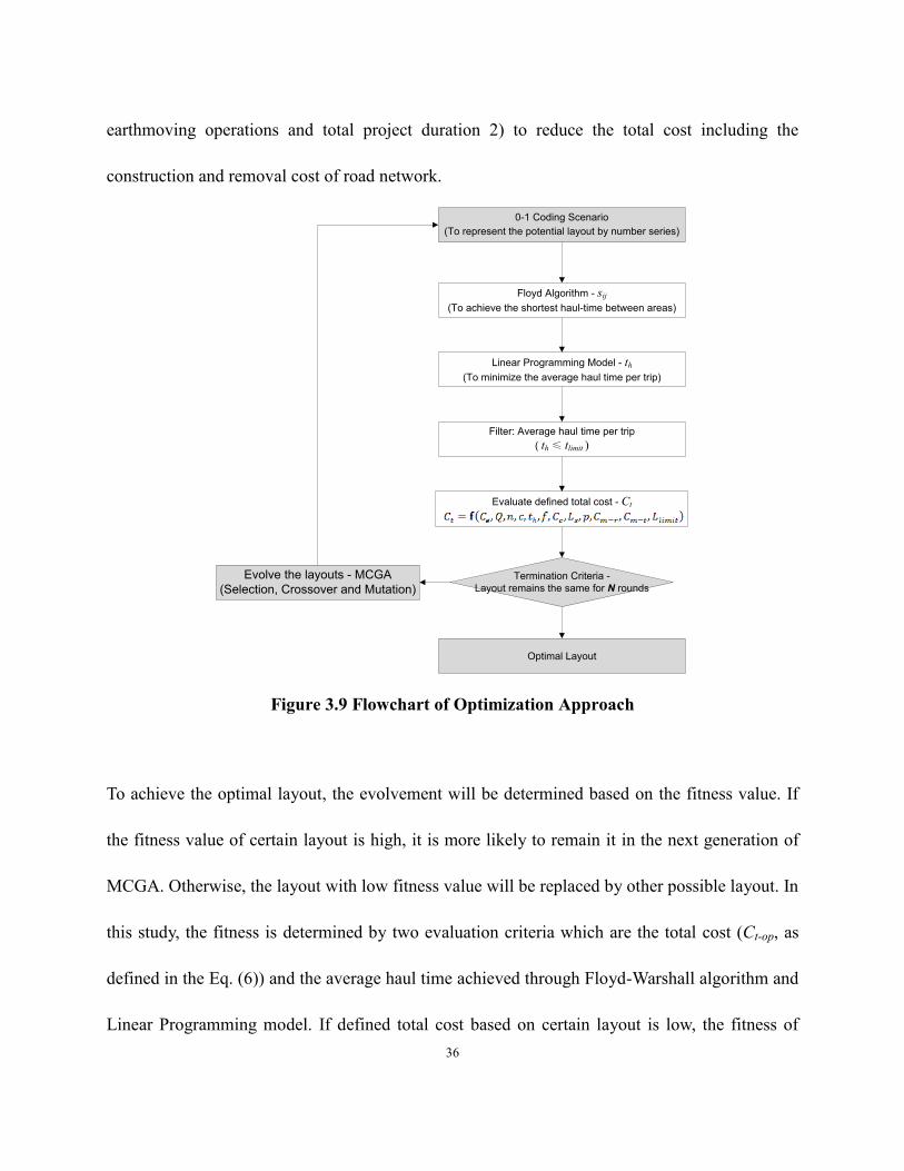
The flowchart of MCGA algorithm which is illustrated in Figure 3.9 indicates details in the

proposed optimization. After inputting the data including the earthwork design, the parameters of

genetic algorithm and empirical parameters of the objective function, the algorithm starts to

search for the optimized temporary road network. All the possible layout of temporary road

network is considered. When the termination criteria are reached, the optimal layout is obtained.

The purpose to achieve the optimized temporary haul road network is 1) to accelerate the

36

earthmoving operations and total project duration 2) to reduce the total cost including the

construction and removal cost of road network.

0-1 Coding Scenario

(To represent the potential layout by number series)

Floyd Algorithm - sij

(To achieve the shortest haul-time between areas)

Linear Programming Model - th

(To minimize the average haul time per trip)

Filter: Average haul time per trip

( th ≤ tlimit )

Evaluate defined total cost - Ct

Evolve the layouts - MCGA

(Selection, Crossover and Mutation)Termination Criteria -

Layout remains the same for N rounds

Optimal Layout

Figure 3.9 Flowchart of Optimization Approach

To achieve the optimal layout, the evolvement will be determined based on the fitness value. If

the fitness value of certain layout is high, it is more likely to remain it in the next generation of

MCGA. Otherwise, the layout with low fitness value will be replaced by other possible layout. In

this study, the fitness is determined by two evaluation criteria which are the total cost (Ct-op, as

defined in the Eq. (6)) and the average haul time achieved through Floyd-Warshall algorithm and

Linear Programming model. If defined total cost based on certain layout is low, the fitness of

37

layout will be high and it is more likely to be the optimal layout. If the average haul time based

on certain layout is beyond expected limit of average haul time, although defined total cost is low,

the fitness of the layout will be defined as zero and it will not become the optimal layout.

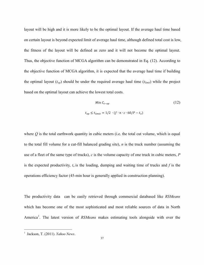
Thus, the objective function of MCGA algorithm can be demonstrated in Eq. (12). According to

the objective function of MCGA algorithm, it is expected that the average haul time if building

the optimal layout (top) should be under the required average haul time (tlimit) while the project

based on the optimal layout can achieve the lowest total costs.

𝑀 𝑛 𝐶𝑡−𝑜𝑝 (12)

𝑡𝑜𝑝 ≤ 𝑡𝑙𝑖𝑚𝑖𝑡 ∙ (𝑓 ∙ 𝑛 ∙ 𝑐 ∙ 𝑃 𝑡𝑜)

where Q is the total earthwork quantity in cubic meters (i.e. the total cut volume, which is equal

to the total fill volume for a cut-fill balanced grading site), n is the truck number (assuming the

use of a fleet of the same type of trucks), c is the volume capacity of one truck in cubic meters, P

is the expected productivity, to is the loading, dumping and waiting time of trucks and f is the

operations efficiency factor (45-min hour is generally applied in construction planning).

The productivity data can be easily retrieved through commercial databased like RSMeans

which has become one of the most sophisticated and most reliable sources of data in North

America1. The latest version of RSMeans makes estimating tools alongside with over the

1 Jackson, T. (2011). Yahoo News.

38

network storage and the archival of cost data on an Internet-based platform. Also, RSMeans

classifies methods by MasterFormat 2010 and publishes data including material cost, labor crew

rates, equipment rates, productivity information and market variations. Thus, to be aligned with

the productivity data definition for typical earthmoving methods as found in databases like

RSMeans, the proposed equation can be easily applied in real practice. (Refer to P52 for an

example in the case study).

Through the proposed approaches, from random starting points, the optimized layout of

temporary road network can be finally derived from alternatives. It is noteworthy that the

variable in the MCGA algorithm is a number series representing the layout of road network. In

short, in connection with each solution of the objective function, the Floyd-Warshall algorithm

along with the linear programming model is applied to any possible layout to determine its

average haul time and optimized earthmoving plan. The computing time of proposed

optimization approaches mainly depends on the problem size. For the small-scale optimization

where the field is divided into dozen cells, the computing time can be within minutes. However,

for the large-scale optimization where complicated earthmoving field is divided into more than

50 cells, the computing time can be in the order of hours.

<http://www.reedconstructiondata.com/Market-Intelligence/Articles/2011/11/RSMeans-Longest-

running-Publication-Building-Construction-Cost-Data-Celebrates-70-Years-RCD010936W/>

39

4 Case Study

4.1 Practical Application to Achieve Optimized Earthmoving Plan

To illustrate the application of the proposed methodology, a practical case is used to evaluate the

performance of the optimized earthmoving job plan based on a particular layout of the temporary

haul road network. The rough grading project is the preliminary work of a campsite construction

in northern Alberta, the site area of which is around 120 hectares. The survey data for the original

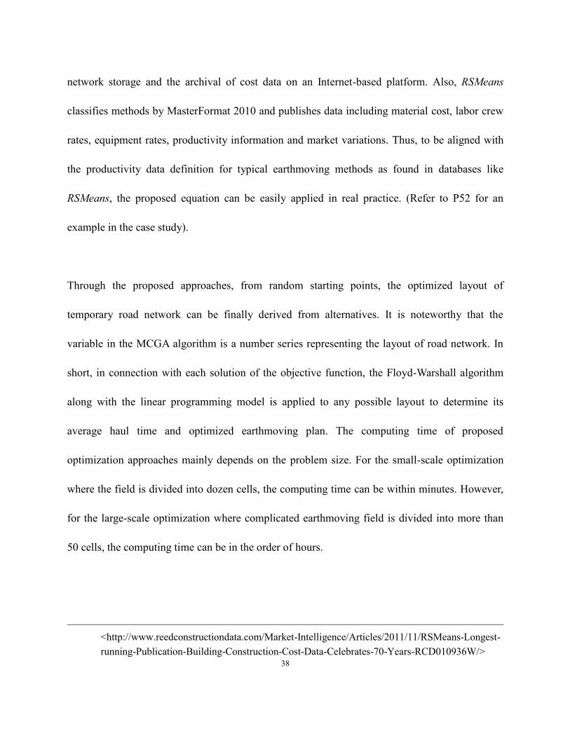
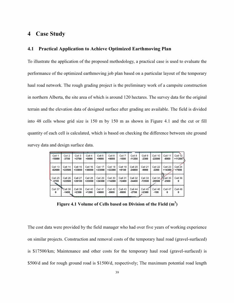
terrain and the elevation data of designed surface after grading are available. The field is divided

into 48 cells whose grid size is 150 m by 150 m as shown in Figure 4.1 and the cut or fill

quantity of each cell is calculated, which is based on checking the difference between site ground

survey data and design surface data.

Figure 4.1 Volume of Cells based on Division of the Field (m3)

The cost data were provided by the field manager who had over five years of working experience

on similar projects. Construction and removal costs of the temporary haul road (gravel-surfaced)

is $17500/km; Maintenance and other costs for the temporary haul road (gravel-surfaced) is

$500/d and for rough ground road is $1500/d, respectively; The maximum potential road length

40

within the entire site area is 5000 m; Mean truck-haul speed on temporary haul road is 36 km/h;

Mean haul speed on rough ground is 24 km/h; Truck volume capacity is 40 m3; Hourly cost of

equipment and crew is $5000/h; Working efficiency factor is 0.75; 8 trucks of the same type

make up the fleet. Based on the cost data, Eq. (13) to (16) can be evaluated for the purpose of

cost-benefit analysis. The total cost (Ct) is essentially a function depending on two variables,

namely: th (the average unit haul time in hour) and L (the total length of temporary

gravel-surfaced haul road in meter).

𝑇 𝑚3 ( ∙ 𝑚3) ∙ 𝑡ℎ . (13)

𝐶𝑡ℎ $ ℎ ∙ 𝑇 (14)

𝐶𝑟𝑛 $ 𝑚 ∙ 𝐿 + 𝐿 𝑚 ∙ $ ∙ 𝑇 + ( 𝐿 𝑚) ∙ $ ∙ 𝑇 (15)

𝐶𝑡 $ . ℎ ∙ . ∙ 𝑡ℎ + $ . 𝑚 ∙ 𝐿 𝐿 𝑚 ∙ $ ℎ ∙ . ∙ 𝑡ℎ (16)

4.1.1 Comparison between Layout Options

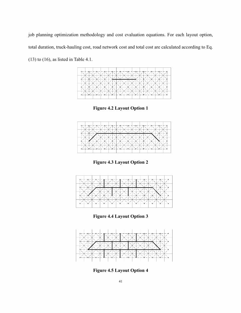
Based on input and empirical data from the site manager, comparison was made for four layout

options of the temporary haul road network with varied total length and configuration of

gravel-surfaced haul roads, as demonstrated with solid line sections in Figure 4.2 to Figure 4.5.

Among the four options, option 1 has the shortest total length of gravel-surfaced haul roads (450

m) with the simplest layout design; while option 4 features the longest gravel-surfaced haul road

(4024 m) and the most complicated configuration. The decision maker intends to identify the

layout option associated with the lowest total cost, by implementing the proposed earthmoving

41

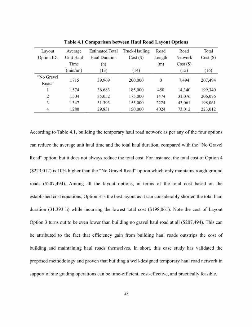
job planning optimization methodology and cost evaluation equations. For each layout option,

total duration, truck-hauling cost, road network cost and total cost are calculated according to Eq.

(13) to (16), as listed in Table 4.1.

Figure 4.2 Layout Option 1

Figure 4.3 Layout Option 2

Figure 4.4 Layout Option 3

Figure 4.5 Layout Option 4

42

Table 4.1 Comparison between Haul Road Layout Options

Layout

Option ID.

Average

Unit Haul

Time

(min/m3)

Estimated Total

Haul Duration

(h)

(13)

Truck-Hauling

Cost ($)

(14)

Road

Length

(m)

Road

Network

Cost ($)

(15)

Total

Cost ($)

(16)

“No Gravel

Road” 1.715 39.969 200,000 0 7,494 207,494

1 1.574 36.683 185,000 450 14,340 199,340

2 1.504 35.052 175,000 1474 31,076 206,076

3 1.347 31.393 155,000 2224 43,061 198,061

4 1.280 29.831 150,000 4024 73,012 223,012

According to Table 4.1, building the temporary haul road network as per any of the four options

can reduce the average unit haul time and the total haul duration, compared with the “No Gravel

Road” option; but it does not always reduce the total cost. For instance, the total cost of Option 4

($223,012) is 10% higher than the “No Gravel Road” option which only maintains rough ground

roads ($207,494). Among all the layout options, in terms of the total cost based on the

established cost equations, Option 3 is the best layout as it can considerably shorten the total haul

duration (31.393 h) while incurring the lowest total cost ($198,061). Note the cost of Layout

Option 3 turns out to be even lower than building no gravel haul road at all ($207,494). This can

be attributed to the fact that efficiency gain from building haul roads outstrips the cost of

building and maintaining haul roads themselves. In short, this case study has validated the

proposed methodology and proven that building a well-designed temporary haul road network in

support of site grading operations can be time-efficient, cost-effective, and practically feasible.

43

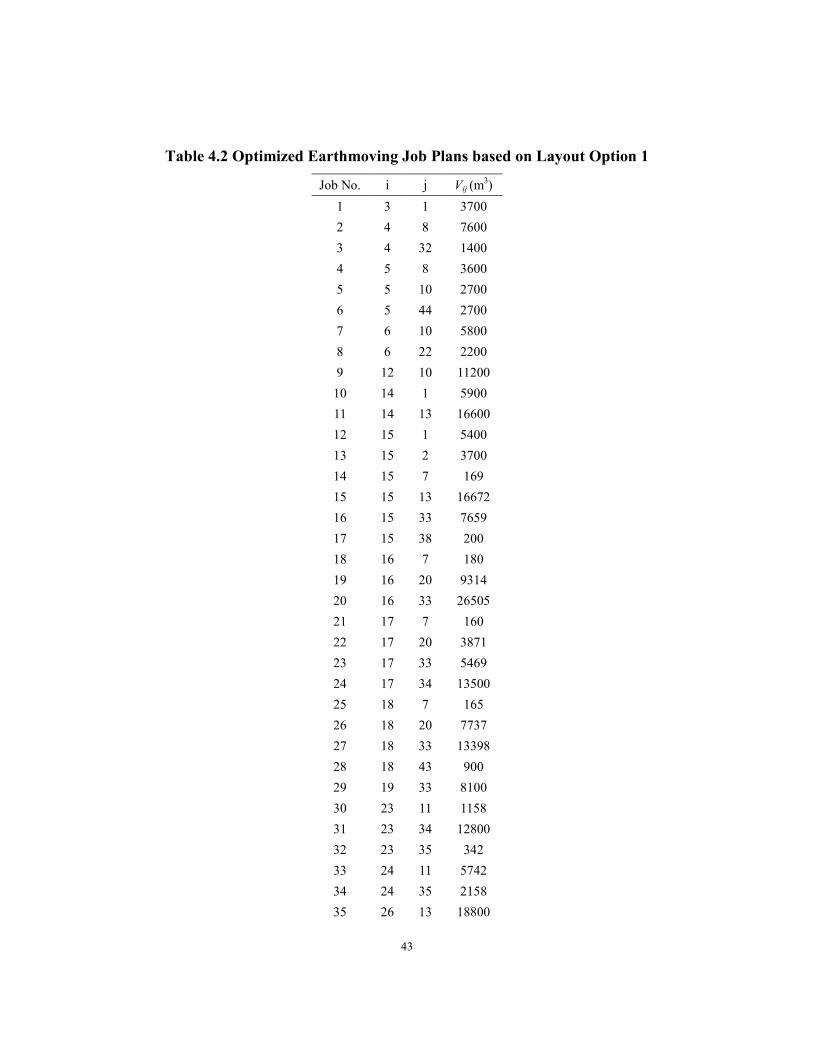
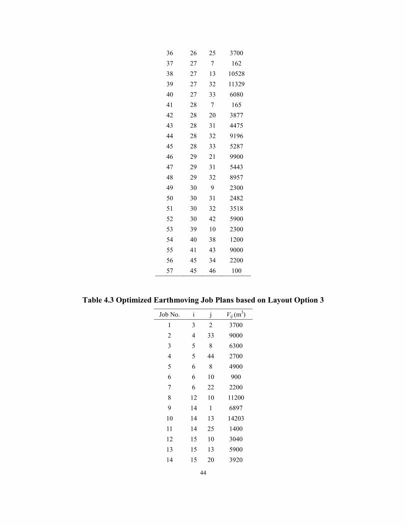
Table 4.2 Optimized Earthmoving Job Plans based on Layout Option 1

Job No. i j Vij (m3)

1 3 1 3700

2 4 8 7600

3 4 32 1400

4 5 8 3600

5 5 10 2700

6 5 44 2700

7 6 10 5800

8 6 22 2200

9 12 10 11200

10 14 1 5900

11 14 13 16600

12 15 1 5400

13 15 2 3700

14 15 7 169

15 15 13 16672

16 15 33 7659

17 15 38 200

18 16 7 180

19 16 20 9314

20 16 33 26505

21 17 7 160

22 17 20 3871

23 17 33 5469

24 17 34 13500

25 18 7 165

26 18 20 7737

27 18 33 13398

28 18 43 900

29 19 33 8100

30 23 11 1158

31 23 34 12800

32 23 35 342

33 24 11 5742

34 24 35 2158

35 26 13 18800

44

36 26 25 3700

37 27 7 162

38 27 13 10528

39 27 32 11329

40 27 33 6080

41 28 7 165

42 28 20 3877

43 28 31 4475

44 28 32 9196

45 28 33 5287

46 29 21 9900

47 29 31 5443

48 29 32 8957

49 30 9 2300

50 30 31 2482

51 30 32 3518

52 30 42 5900

53 39 10 2300

54 40 38 1200

55 41 43 9000

56 45 34 2200

57 45 46 100

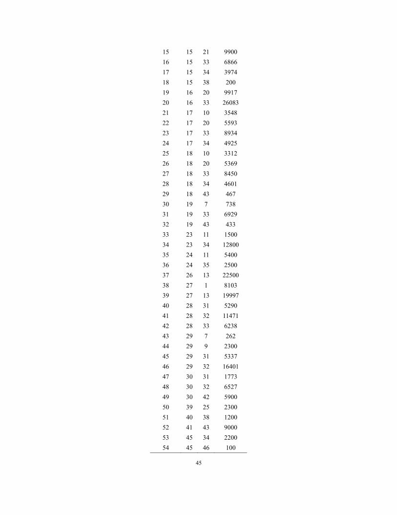
Table 4.3 Optimized Earthmoving Job Plans based on Layout Option 3

Job No. i j Vij (m3)

1 3 2 3700

2 4 33 9000

3 5 8 6300

4 5 44 2700

5 6 8 4900

6 6 10 900

7 6 22 2200

8 12 10 11200

9 14 1 6897

10 14 13 14203

11 14 25 1400

12 15 10 3040

13 15 13 5900

14 15 20 3920

45

15 15 21 9900

16 15 33 6866

17 15 34 3974

18 15 38 200

19 16 20 9917

20 16 33 26083

21 17 10 3548

22 17 20 5593

23 17 33 8934

24 17 34 4925

25 18 10 3312

26 18 20 5369

27 18 33 8450

28 18 34 4601

29 18 43 467

30 19 7 738

31 19 33 6929

32 19 43 433

33 23 11 1500

34 23 34 12800

35 24 11 5400

36 24 35 2500

37 26 13 22500

38 27 1 8103

39 27 13 19997

40 28 31 5290

41 28 32 11471

42 28 33 6238

43 29 7 262

44 29 9 2300

45 29 31 5337

46 29 32 16401

47 30 31 1773

48 30 32 6527

49 30 42 5900

50 39 25 2300

51 40 38 1200

52 41 43 9000

53 45 34 2200

54 45 46 100

46

Further scrutiny of the optimized earthmoving plans resulting from option 3 and option 4 leads to

one additional observation critical to earthmoving job planning: option 3 (54 jobs) reduces both

the minimized average haul time and the total job number when compared with layout option 1

(57 jobs). With three fewer jobs, option 3 can significantly reduce site mobilization efforts and

facilitate earthmoving operations, thus is preferred over option 1 from the perspective of field

execution. As a result, layout option 3 is deemed the best layout among the four options. In

reality, the total costs for option 1 and option 3 are close, so the optimized earthmoving plans

associated with the two options, listed in Table 4.2 and Table 4.3, can be both presented to the

field personnel, who would make the final choice by further evaluating the feasibility of field

implementation. In short, the proposed approach lends effective, transparent decision support to

guide practitioners in earthmoving job planning, temporary haul road network design and job

plan execution.

4.1.2 Effect of Grid Size Selection

As mentioned in the previous section, the distance between two access roads mainly decides the

grid size and 150 m is recommended as a proper choice. In order to shed light on the selection of

the grid size suitable for practical application, results from analyzing three cases with different

grid sizes (150 m, 200 m, 300 m) based on layout option 1 and layout option 3 are presented and

compared. The proposed methodology was repeated on two additional grid-size scenarios and the

47

final results are compared against the base-case scenario (150 m grid size), shown in Table 4.2

and Table 4.3 for layout option 1 and layout option 3, respectively.

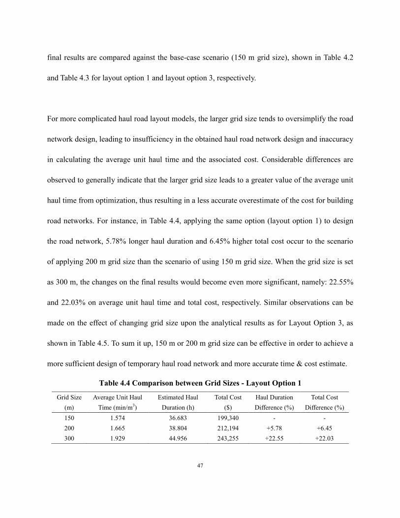
For more complicated haul road layout models, the larger grid size tends to oversimplify the road

network design, leading to insufficiency in the obtained haul road network design and inaccuracy

in calculating the average unit haul time and the associated cost. Considerable differences are

observed to generally indicate that the larger grid size leads to a greater value of the average unit

haul time from optimization, thus resulting in a less accurate overestimate of the cost for building

road networks. For instance, in Table 4.4, applying the same option (layout option 1) to design

the road network, 5.78% longer haul duration and 6.45% higher total cost occur to the scenario

of applying 200 m grid size than the scenario of using 150 m grid size. When the grid size is set

as 300 m, the changes on the final results would become even more significant, namely: 22.55%

and 22.03% on average unit haul time and total cost, respectively. Similar observations can be

made on the effect of changing grid size upon the analytical results as for Layout Option 3, as

shown in Table 4.5. To sum it up, 150 m or 200 m grid size can be effective in order to achieve a

more sufficient design of temporary haul road network and more accurate time & cost estimate.

Table 4.4 Comparison between Grid Sizes - Layout Option 1

Grid Size

(m)

Average Unit Haul

Time (min/m3)

Estimated Haul

Duration (h)

Total Cost

($)

Haul Duration

Difference (%)

Total Cost

Difference (%)

150 1.574 36.683 199,340 - -

200 1.665 38.804 212,194 +5.78 +6.45

300 1.929 44.956 243,255 +22.55 +22.03

48

Table 4.5 Comparison between Grid Sizes - Layout Option 3

Grid Size

(m)

Average Unit Haul

Time (min/m3)

Estimated Haul

Duration (h)

Total Cost

($)

Haul Duration

Difference (%)

Total Cost

Difference (%)

150 1.347 31.393 198,061 - -

200 1.471 34.282 212,477 +9.20 +7.28

300 1.652 38.501 236,948 +22.64 +19.63

4.1.3 Summary

In this section, the proposed method has successfully applied to a practical earthmoving case in

northern Alberta. Previous research has not yet deliberately addressed how to optimize

earthmoving operations planning in connection with the layout design of temporary haul road

networks for mass earthworks projects. The research has introduced concepts in transportation

engineering into the construction domain (such as formulating the design of temporary haul road

networks into grid model, the Floyd-Warshall algorithm for network planning optimization.) The

present research has proposed a quantitative methodology for optimizing earthmoving job

planning based on evaluation of the road network design during the detailed construction

planning stage. Through seamless integration of Floyd-Warshall algorithm and Linear

Programming model, the shortest average unit haul time along with earthmoving plan can be

obtained while automatically fulfilling site grading design specifications. Each job is defined in

terms of the source cell, the destination cell, the earth volume, and the shortest-hauling-time path

between source and destination. To some extent, the proposed methodology converts an

empirical planning issue in construction engineering into an analytical problem, amenable to

formulating quantitative solutions.

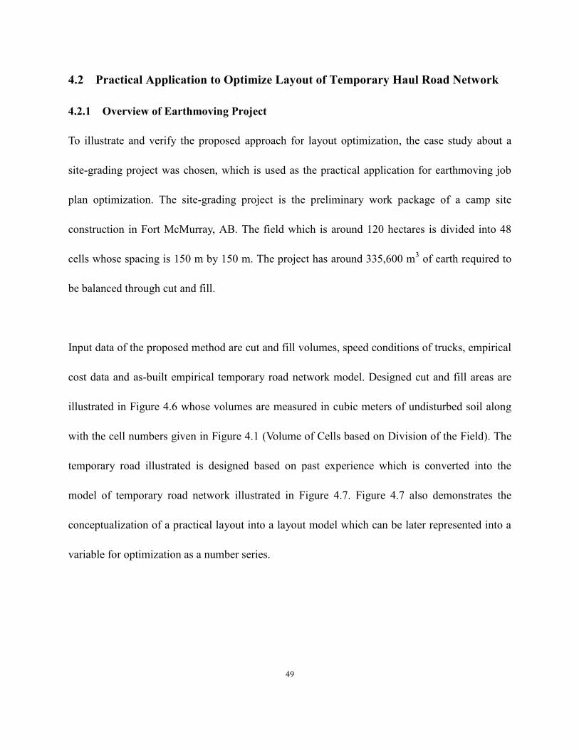
49

4.2 Practical Application to Optimize Layout of Temporary Haul Road Network

4.2.1 Overview of Earthmoving Project

To illustrate and verify the proposed approach for layout optimization, the case study about a

site-grading project was chosen, which is used as the practical application for earthmoving job

plan optimization. The site-grading project is the preliminary work package of a camp site

construction in Fort McMurray, AB. The field which is around 120 hectares is divided into 48

cells whose spacing is 150 m by 150 m. The project has around 335,600 m3 of earth required to

be balanced through cut and fill.

Input data of the proposed method are cut and fill volumes, speed conditions of trucks, empirical

cost data and as-built empirical temporary road network model. Designed cut and fill areas are

illustrated in Figure 4.6 whose volumes are measured in cubic meters of undisturbed soil along

with the cell numbers given in Figure 4.1 (Volume of Cells based on Division of the Field). The

temporary road illustrated is designed based on past experience which is converted into the

model of temporary road network illustrated in Figure 4.7. Figure 4.7 also demonstrates the

conceptualization of a practical layout into a layout model which can be later represented into a

variable for optimization as a number series.

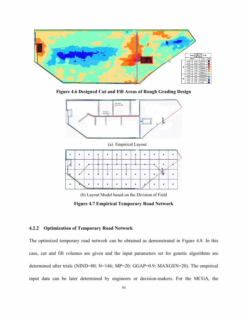
50

Figure 4.6 Designed Cut and Fill Areas of Rough Grading Design

(a) Empirical Layout

(b) Layout Model based on the Division of Field

Figure 4.7 Empirical Temporary Road Network

4.2.2 Optimization of Temporary Road Network

The optimized temporary road network can be obtained as demonstrated in Figure 4.8. In this

case, cut and fill volumes are given and the input parameters set for genetic algorithms are

determined after trials (NIND=80; N=146; MP=20; GGAP=0.9; MAXGEN=20). The empirical

input data can be later determined by engineers or decision-makers. For the MCGA, the

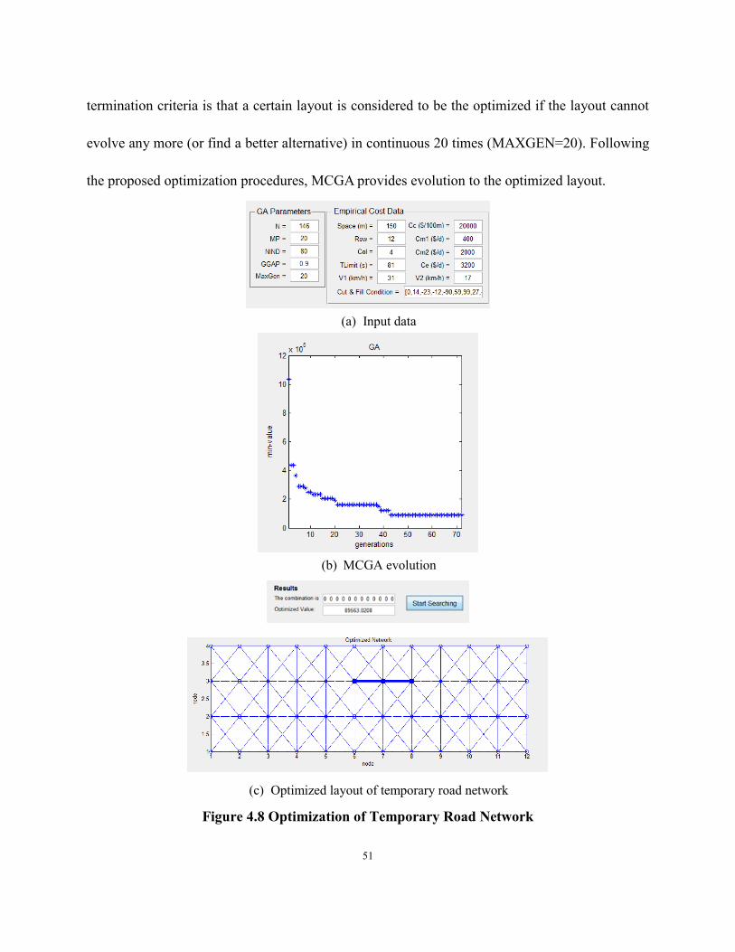
51

termination criteria is that a certain layout is considered to be the optimized if the layout cannot

evolve any more (or find a better alternative) in continuous 20 times (MAXGEN=20). Following

the proposed optimization procedures, MCGA provides evolution to the optimized layout.

(a) Input data

(b) MCGA evolution

(c) Optimized layout of temporary road network

Figure 4.8 Optimization of Temporary Road Network

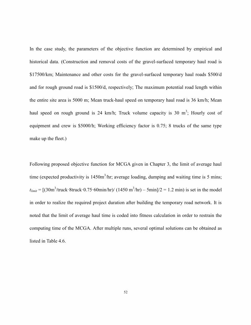
52

In the case study, the parameters of the objective function are determined by empirical and

historical data. (Construction and removal costs of the gravel-surfaced temporary haul road is

$17500/km; Maintenance and other costs for the gravel-surfaced temporary haul roads $500/d

and for rough ground road is $1500/d, respectively; The maximum potential road length within

the entire site area is 5000 m; Mean truck-haul speed on temporary haul road is 36 km/h; Mean

haul speed on rough ground is 24 km/h; Truck volume capacity is 30 m3; Hourly cost of

equipment and crew is $5000/h; Working efficiency factor is 0.75; 8 trucks of the same type

make up the fleet.)

Following proposed objective function for MCGA given in Chapter 3, the limit of average haul

time (expected productivity is 1450m3/hr; average loading, dumping and waiting time is 5 mins;

tlimit = [(30m3/truck·8truck·0.75·60min/hr)/ (1450 m

3/hr) – 5min]/2 = 1.2 min) is set in the model

in order to realize the required project duration after building the temporary road network. It is

noted that the limit of average haul time is coded into fitness calculation in order to restrain the

computing time of the MCGA. After multiple runs, several optimal solutions can be obtained as

listed in Table 4.6.

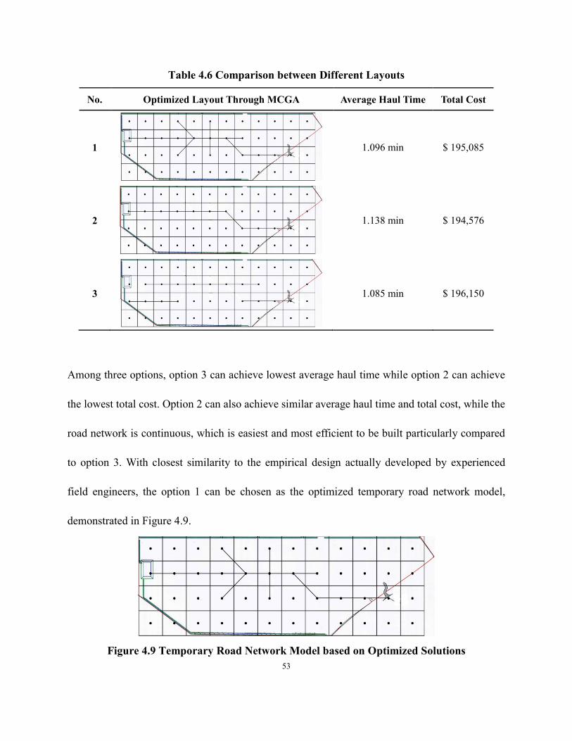
53

Table 4.6 Comparison between Different Layouts

No. Optimized Layout Through MCGA Average Haul Time Total Cost

1

1.096 min $ 195,085

2

1.138 min $ 194,576

3

1.085 min $ 196,150

Among three options, option 3 can achieve lowest average haul time while option 2 can achieve

the lowest total cost. Option 2 can also achieve similar average haul time and total cost, while the

road network is continuous, which is easiest and most efficient to be built particularly compared

to option 3. With closest similarity to the empirical design actually developed by experienced

field engineers, the option 1 can be chosen as the optimized temporary road network model,

demonstrated in Figure 4.9.

Figure 4.9 Temporary Road Network Model based on Optimized Solutions

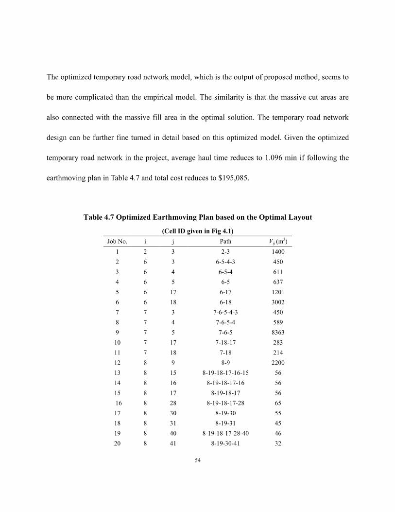
54

The optimized temporary road network model, which is the output of proposed method, seems to

be more complicated than the empirical model. The similarity is that the massive cut areas are

also connected with the massive fill area in the optimal solution. The temporary road network

design can be further fine turned in detail based on this optimized model. Given the optimized

temporary road network in the project, average haul time reduces to 1.096 min if following the

earthmoving plan in Table 4.7 and total cost reduces to $195,085.

Table 4.7 Optimized Earthmoving Plan based on the Optimal Layout

(Cell ID given in Fig 4.1)

Job No. i j Path Vij (m3)

1 2 3 2-3 1400

2 6 3 6-5-4-3 450

3 6 4 6-5-4 611

4 6 5 6-5 637

5 6 17 6-17 1201

6 6 18 6-18 3002

7 7 3 7-6-5-4-3 450

8 7 4 7-6-5-4 589

9 7 5 7-6-5 8363

10 7 17 7-18-17 283

11 7 18 7-18 214

12 8 9 8-9 2200

13 8 15 8-19-18-17-16-15 56

14 8 16 8-19-18-17-16 56

15 8 17 8-19-18-17 56

16 8 28 8-19-18-17-28 65

17 8 30 8-19-30 55

18 8 31 8-19-31 45

19 8 40 8-19-18-17-28-40 46

20 8 41 8-19-30-41 32

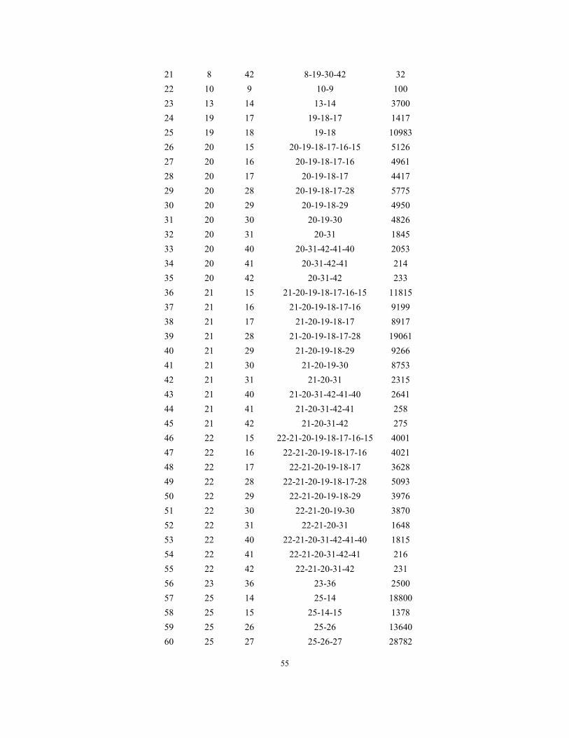
55

21 8 42 8-19-30-42 32

22 10 9 10-9 100

23 13 14 13-14 3700

24 19 17 19-18-17 1417

25 19 18 19-18 10983

26 20 15 20-19-18-17-16-15 5126

27 20 16 20-19-18-17-16 4961

28 20 17 20-19-18-17 4417

29 20 28 20-19-18-17-28 5775

30 20 29 20-19-18-29 4950

31 20 30 20-19-30 4826

32 20 31 20-31 1845

33 20 40 20-31-42-41-40 2053

34 20 41 20-31-42-41 214

35 20 42 20-31-42 233

36 21 15 21-20-19-18-17-16-15 11815

37 21 16 21-20-19-18-17-16 9199

38 21 17 21-20-19-18-17 8917

39 21 28 21-20-19-18-17-28 19061

40 21 29 21-20-19-18-29 9266

41 21 30 21-20-19-30 8753

42 21 31 21-20-31 2315

43 21 40 21-20-31-42-41-40 2641

44 21 41 21-20-31-42-41 258

45 21 42 21-20-31-42 275

46 22 15 22-21-20-19-18-17-16-15 4001

47 22 16 22-21-20-19-18-17-16 4021

48 22 17 22-21-20-19-18-17 3628

49 22 28 22-21-20-19-18-17-28 5093

50 22 29 22-21-20-19-18-29 3976

51 22 30 22-21-20-19-30 3870

52 22 31 22-21-20-31 1648

53 22 40 22-21-20-31-42-41-40 1815

54 22 41 22-21-20-31-42-41 216

55 22 42 22-21-20-31-42 231

56 23 36 23-36 2500

57 25 14 25-14 18800

58 25 15 25-14-15 1378

59 25 26 25-26 13640

60 25 27 25-26-27 28782

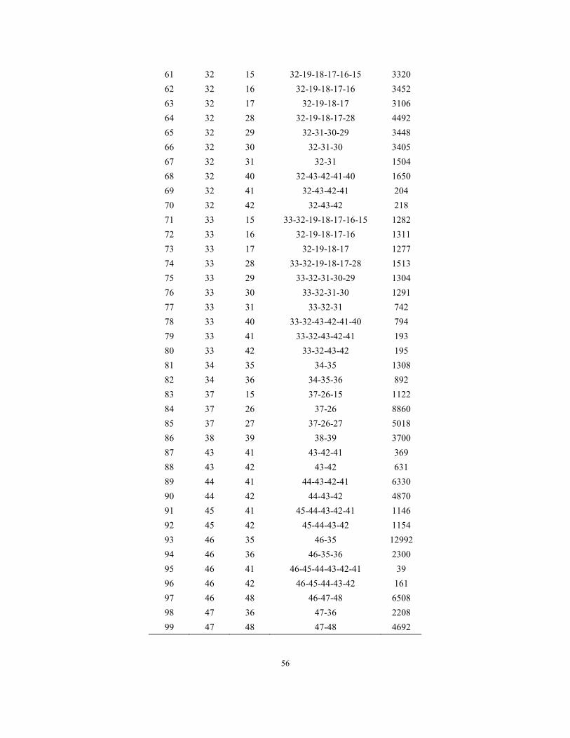
56

61 32 15 32-19-18-17-16-15 3320

62 32 16 32-19-18-17-16 3452

63 32 17 32-19-18-17 3106

64 32 28 32-19-18-17-28 4492

65 32 29 32-31-30-29 3448

66 32 30 32-31-30 3405

67 32 31 32-31 1504

68 32 40 32-43-42-41-40 1650

69 32 41 32-43-42-41 204

70 32 42 32-43-42 218

71 33 15 33-32-19-18-17-16-15 1282

72 33 16 32-19-18-17-16 1311

73 33 17 32-19-18-17 1277

74 33 28 33-32-19-18-17-28 1513

75 33 29 33-32-31-30-29 1304

76 33 30 33-32-31-30 1291

77 33 31 33-32-31 742

78 33 40 33-32-43-42-41-40 794

79 33 41 33-32-43-42-41 193

80 33 42 33-32-43-42 195

81 34 35 34-35 1308

82 34 36 34-35-36 892

83 37 15 37-26-15 1122

84 37 26 37-26 8860

85 37 27 37-26-27 5018

86 38 39 38-39 3700

87 43 41 43-42-41 369

88 43 42 43-42 631

89 44 41 44-43-42-41 6330

90 44 42 44-43-42 4870

91 45 41 45-44-43-42-41 1146

92 45 42 45-44-43-42 1154

93 46 35 46-35 12992

94 46 36 46-35-36 2300

95 46 41 46-45-44-43-42-41 39

96 46 42 46-45-44-43-42 161

97 46 48 46-47-48 6508

98 47 36 47-36 2208

99 47 48 47-48 4692

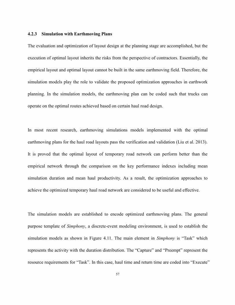
57

4.2.3 Simulation with Earthmoving Plans

The evaluation and optimization of layout design at the planning stage are accomplished, but the

execution of optimal layout inherits the risks from the perspective of contractors. Essentially, the

empirical layout and optimal layout cannot be built in the same earthmoving field. Therefore, the

simulation models play the role to validate the proposed optimization approaches in earthwork

planning. In the simulation models, the earthmoving plan can be coded such that trucks can

operate on the optimal routes achieved based on certain haul road design.

In most recent research, earthmoving simulations models implemented with the optimal

earthmoving plans for the haul road layouts pass the verification and validation (Liu et al. 2013).

It is proved that the optimal layout of temporary road network can perform better than the

empirical network through the comparison on the key performance indexes including mean

simulation duration and mean haul productivity. As a result, the optimization approaches to

achieve the optimized temporary haul road network are considered to be useful and effective.

The simulation models are established to encode optimized earthmoving plans. The general

purpose template of Simphony, a discrete-event modeling environment, is used to establish the

simulation models as shown in Figure 4.11. The main element in Simphony is “Task” which

represents the activity with the duration distribution. The “Capture” and “Preempt” represent the

resource requirements for “Task”. In this case, haul time and return time are coded into “Execute”

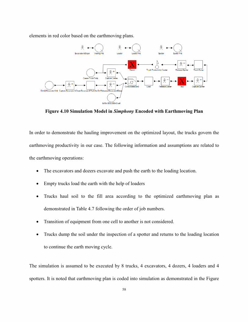
58

elements in red color based on the earthmoving plans.

Figure 4.10 Simulation Model in Simphony Encoded with Earthmoving Plan

In order to demonstrate the hauling improvement on the optimized layout, the trucks govern the

earthmoving productivity in our case. The following information and assumptions are related to

the earthmoving operations:

The excavators and dozers excavate and push the earth to the loading location.

Empty trucks load the earth with the help of loaders

Trucks haul soil to the fill area according to the optimized earthmoving plan as

demonstrated in Table 4.7 following the order of job numbers.

Transition of equipment from one cell to another is not considered.

Trucks dump the soil under the inspection of a spotter and returns to the loading location

to continue the earth moving cycle.

The simulation is assumed to be executed by 8 trucks, 4 excavators, 4 dozers, 4 loaders and 4

spotters. It is noted that earthmoving plan is coded into simulation as demonstrated in the Figure

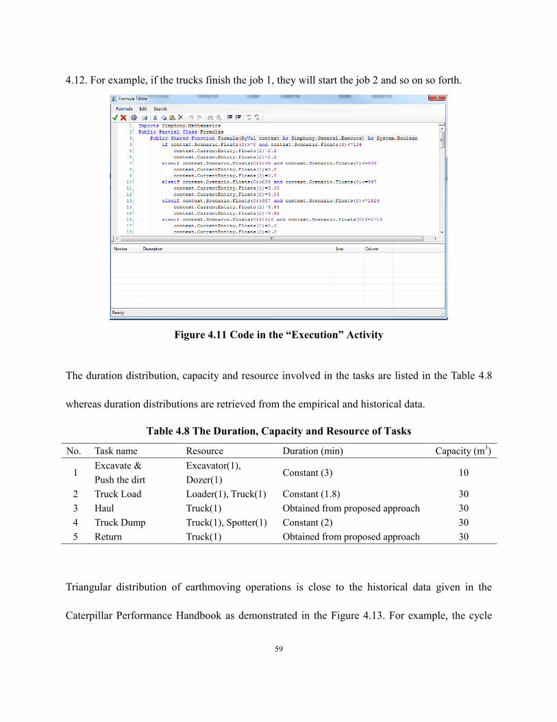
59

4.12. For example, if the trucks finish the job 1, they will start the job 2 and so on so forth.

Figure 4.11 Code in the “Execution” Activity

The duration distribution, capacity and resource involved in the tasks are listed in the Table 4.8

whereas duration distributions are retrieved from the empirical and historical data.

Table 4.8 The Duration, Capacity and Resource of Tasks

No. Task name Resource Duration (min) Capacity (m3)

1 Excavate &

Push the dirt

Excavator(1),

Dozer(1) Constant (3) 10

2 Truck Load Loader(1), Truck(1) Constant (1.8) 30

3 Haul Truck(1) Obtained from proposed approach 30

4 Truck Dump Truck(1), Spotter(1) Constant (2) 30

5 Return Truck(1) Obtained from proposed approach 30

Triangular distribution of earthmoving operations is close to the historical data given in the

Caterpillar Performance Handbook as demonstrated in the Figure 4.13. For example, the cycle

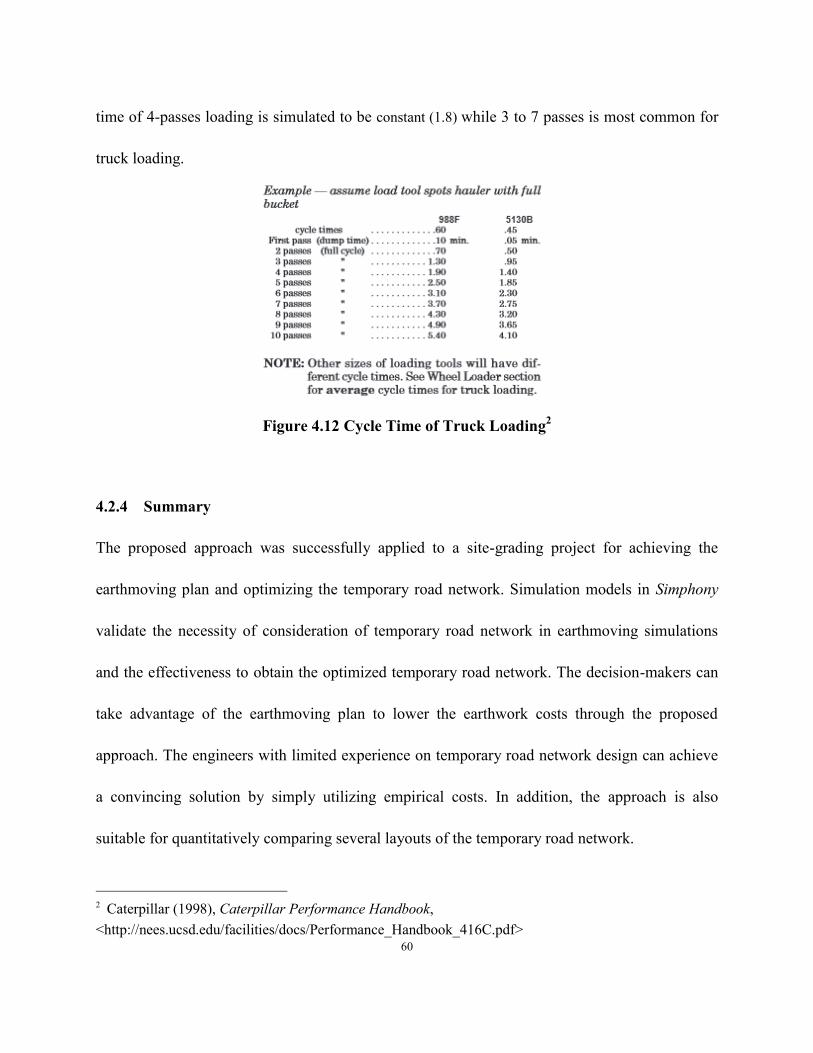
60

time of 4-passes loading is simulated to be constant (1.8) while 3 to 7 passes is most common for

truck loading.

Figure 4.12 Cycle Time of Truck Loading2

4.2.4 Summary

The proposed approach was successfully applied to a site-grading project for achieving the

earthmoving plan and optimizing the temporary road network. Simulation models in Simphony

validate the necessity of consideration of temporary road network in earthmoving simulations

and the effectiveness to obtain the optimized temporary road network. The decision-makers can

take advantage of the earthmoving plan to lower the earthwork costs through the proposed

approach. The engineers with limited experience on temporary road network design can achieve

a convincing solution by simply utilizing empirical costs. In addition, the approach is also

suitable for quantitatively comparing several layouts of the temporary road network.

2 Caterpillar (1998), Caterpillar Performance Handbook,

<http://nees.ucsd.edu/facilities/docs/Performance_Handbook_416C.pdf>

61

As the optimization approach cannot be detached from the empirical cost data and the conceptual

model of temporary road network, it is foreseen that there is a need to improve the reliability of

empirical cost data to achieve better optimized solutions. The space of cells varies depending on

conditions of test cases which should be further studied. In addition, the efficiency of the

optimization algorithm can be improved, which depends on complexity of the problem definition.

The further improvement of the proposed approach would be worthy of research to help

construction managers rely on a controllable and analytical method rather than experience for

critical decision making in earthmoving planning.

4.3 Validation of Layout Optimization Approach

If earthmoving simulations encoded with earthmoving plans pass verification and validation, the

entire optimization approach can be deemed useful. By comparing the minimized average haul

time, total duration and total cost, the optimized temporary road network performs better than the

empirical network. In order to validate the optimization approach, three simulation models

encoded with corresponding earthmoving plan are developed as follows:

1. Model encoded with earthmoving plan considering rough ground (no temporary road).

2. Model encoded with earthmoving plan considering empirical temporary road network.

3. Model encoded with earthmoving plan considering optimized temporary road network 1.

4. Model encoded with earthmoving plan considering optimized temporary road network 2.

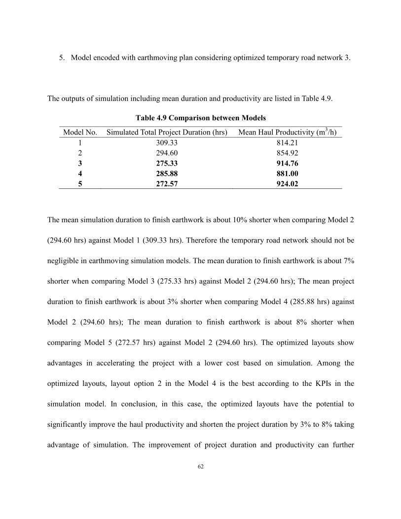
62

5. Model encoded with earthmoving plan considering optimized temporary road network 3.

The outputs of simulation including mean duration and productivity are listed in Table 4.9.

Table 4.9 Comparison between Models

Model No. Simulated Total Project Duration (hrs) Mean Haul Productivity (m3/h)

1 309.33 814.21

2 294.60 854.92

3 275.33 914.76

4 285.88 881.00

5 272.57 924.02

The mean simulation duration to finish earthwork is about 10% shorter when comparing Model 2

(294.60 hrs) against Model 1 (309.33 hrs). Therefore the temporary road network should not be

negligible in earthmoving simulation models. The mean duration to finish earthwork is about 7%

shorter when comparing Model 3 (275.33 hrs) against Model 2 (294.60 hrs); The mean project

duration to finish earthwork is about 3% shorter when comparing Model 4 (285.88 hrs) against

Model 2 (294.60 hrs); The mean duration to finish earthwork is about 8% shorter when

comparing Model 5 (272.57 hrs) against Model 2 (294.60 hrs). The optimized layouts show

advantages in accelerating the project with a lower cost based on simulation. Among the

optimized layouts, layout option 2 in the Model 4 is the best according to the KPIs in the

simulation model. In conclusion, in this case, the optimized layouts have the potential to

significantly improve the haul productivity and shorten the project duration by 3% to 8% taking

advantage of simulation. The improvement of project duration and productivity can further

63

benefit the contractor to reduce the fleet size if handling several earthworks at the same time.

4.4 Cost Saving of Optimization Method

Based on the simulation models, the analytical layout optimization method can increase the total

productivity by 3% to 8%, when compared against the empirical layout design method. The

increase of productivity will directly result in savings on total project duration and cost.

However, the total cost saving based on proposed optimization approaches can be far beyond the

magnitude of 3% to 8%, which is very conservative estimate and only accounts for the saving in

terms of truck hauling time and cost resulting from haul road network design optimization. For

inexperienced personnel, the improvement based on the optimization approach can be very

significant. Although experienced personnel can get close to the optimal design, they can be

further helped with earthmoving job plan optimization to save on operation time and cost. The

total saving resulting from the proposed framework implementing both layout design

optimization and earthmoving job planning optimization will be assessed through formal field

based or simulation based studies in the future.

64

5 Conclusions and Further Research

5.1 Conclusions

In reality, the goal of building the temporary haul road network is to accelerate project progress

without significantly increasing project cost. The research adds to the existing body of

knowledge by defining a cost function as an effective performance measurement of the

temporary haul road network design, based on the average unit haul time, direct truck-hauling

crew cost, and indirect costs for constructing and maintaining haul roads of various types. As

such, the associated cost of executing the optimized earthmoving plan over a particular

temporary haul road networks design can be readily estimated, making it straightforward for

project managers to compare feasible alternatives. The research deliverables will potentially be

of immediate use in practice and cater to the needs of earthworks contractors in terms of

enhancing current practices of planning earthmoving operations and designing temporary haul

road networks.

Analogous to the site grading design, the haul road network design is also based on a rectangular

grid system with a larger width that is applied to geometrically profile the site. Thus, the haul

road alignment design is constrained by the granularity of the grid system; curved alignment can

only be approximated by linking the centroids of two adjacent cells diagonally. In addition,

traffic control measures at intersections in the haul road network, such as yield/stop signs or

traffic lights are ignored in the present research due to the relatively light traffic volume in

65

comparison with the permanent road network design.

With application examples, the proposed methodology has justified that a well-designed

temporary road network can be time-efficient, cost-effective, thus worthy to be built. It is

emphasized that the proposed methodology for earthmoving job planning, haul road design, and

time-cost evaluation of operations only adds to knowhow and experience of practitioners,

providing decision support to enable them to improve performances in day-by-day practice.

The main contributions of this study include 1) adapting established concepts in transportation

engineering domain for practical applications in the construction engineering domain; 2)

improving earthmoving operations by factoring in the temporary haul road network which is not

taken seriously in previous research efforts; 3) converting an empirical temporary road planning

problem into an analytical optimization problem as part of earthworks design and earthmoving

operations planning.

In conclusion, the proposed approaches have been successfully applied to the site grading project

for optimizing the earthmoving operations plan and optimizing the temporary road network

design simultaneously. The simulation models established in Simphony are used to show the

necessity of consideration of temporary road networks in earthmoving simulations and validate

the effectiveness of the optimized temporary road network obtained from the proposed research.

66

The planners or decision-makers can take advantage of the optimized results (optimized

earthmoving plan and optimized temporary haul road network) in order to shorten the

earthmoving duration and lower the costs. Junior engineers with limited experience on temporary

road network design can deliver an impressive, practical solution by simply utilizing empirical

cost data. Also, for mass earthworks, the resulting time and cost savings through proposed

methods can obviously improve productivity and profitability for construction companies.

5.2 Limitations

To support critical decision-making in construction engineering, and to convert a purely

empirical planning problem into a quantitative, automated methodology, further improvements

on this research will be worthwhile and discussed as follows:

Earthmoving Field & Rectangular Gird

In the present research, the division of the field is straightforward and is based on the grid model,

making it reasonable to assume the center of each cell to be the centroid of each cell. However,

for the earthmoving fields with irregular shape or boundaries, the grid model to divide the field

requires further study and assumptions.

Cut-and-fill Balanced Design

The earthwork design is one essential input of proposed optimization approach. In the present

67

research, the earthwork design is required to be cut-and-fill balancing design especially for the

linear programming model. For unbalanced designs, preliminary data processing should be made

in order to achieve an “artificial balance.” For example, extra volume can be counted into the

volume of a specific cell on site. It is reasonable to assume that the extra cut volume to be moved

out of the field is treated as the “fill” volume of the entrance cell. Based on reasonable

assumptions, unbalanced designs can be artificially balanced prior to implementing the proposed

methodologies.

Temporary Haul Road Network

In earthmoving projects, due to different purposes to build the haul road, haul road networks can

be categorized into temporary, semi-permanent or permanent. Massive earthwork operations

serve as the preliminary work of construction and usually last several months which only require

a temporary road network. Therefore, if the haul road network is planned to become a permanent

road after completing the earthworks, the optimization approaches require further improvements.

Layout Optimization

The layout optimization in terms of temporary haul road network design is successfully applied

into the case study based on evaluation criteria including total cost and total duration. However,

the constructability of a temporary road network is not considered in the numerical criteria and

the objective function depends on a set of empirical cost data. The objective functions and

68

criteria for layout optimization require refinement in future study.

Earthmoving Fleet Design

The present research assumes a fixed truck fleet (quantity and type of trucks) to be available and

employed in the field and one single type of trucks is employed with the average truck speed

being only determined by the haul road type, regardless of truck being fully-loaded or empty.

Nonetheless, more sophisticated fleet design can be further added to the proposed optimization

problem scope in the future research as such needs arise from practice.

5.3 Future Research

Serving as the decision support tool, the optimization approaches cannot be detached from the

empirical cost data and the conceptual model of temporary road networks, which reside in the

mental model of experienced field personnel. It is foreseen that there is a need to improve the

reliability of empirical cost data in order to achieve better optimized solutions. The space of cells

varies depending on conditions of test cases, which should be further studied. In addition, the

efficiency of the optimization algorithm can be improved, which depends on the complexity of

the problem definition. The constructability is crucial in real practice but it cannot be easily

modelled into objective functions which require deeper thoughts and more sophisticated

modeling. However, the optimization studies make contributions to connecting the transportation

engineering with construction engineering and management. In short, the further improvement of

69

the proposed approach would be well warranted to help construction managers take advantage of

practical yet analytical methods, instead of relying on experiences alone, for critical decision

making in earthmoving planning.

70

References

Alberta Infrastructure and Transportation (2005). "Chapter I Access Management Guidelines",

Highway Geometric Design Guide, <https://www.transportation.alberta.ca/951.htm> (Apr.

25, 2014)

Choi, Y., and A. Nieto (2011). "Optimal haulage routing of off-road dump trucks in construction

and mining sites using Google Earth and a modified least-cost path algorithm", Autom.

Constr., 20(7), 982–997.

Deng, L., Shi, F., and Liang, T. (2007) "Multi-Generation Compete Genetic Algorithms and Its

Application in Vehicle Routing Problem." International Conference on Transportation

Engineering 2007, 3184-3189.

de Lima, R., Júnior, E., de Athayde Prata, B., and Weissmann, J. (2012). "Distribution of

Materials in Road Earthmoving and Paving: A Mathematical Programming Approach." J.

Constr. Eng. Manage., 139(8), 1046–1054.

Dou, F., Yan, K., Huang, Y., Wang, L., and Jia, L. (2014). "Optimal Path Choice

in Railway Passenger Travel Network Based on Residual Train Capacity." The

Scientific World Journal, 2014, 1-8.

Floyd, Robert W. (1962). "Algorithm 97: Shortest Path". Communications of the ACM, 5 (6),

345.

71

Gross, J. L., Yellen, J. (2003), “Handbook of Graph Theory, Discrete Mathematics

and Its Applications.” CRC Press, 62-63.

Hajjar, D., and AbouRizk, S. (1997). “AP2-Earth: A Simulation-Based System for the

Estimating and Planning of Earth Moving Operations.” Winter Simulation Conference,

Atlanta, Georgia, 1103-1110.

Jayawardane, A. and Harris, F. (1990). ”Further Development of Integer Programming in

Earthwork Optimization.” J. Constr. Eng. Manage., 116(1), 18–34.

Ji, Y. , Borrmann, A. , Rank, E. , Seipp, F. , and Ruzika, S. (2010). “Mathematical

modeling of earthwork optimization problems.” Proc. Int. Conf. on Computing

in Civil and Building Engineering, Nottingham Univ. Press, Nottingham, U.K.

Kang, S. and Seo, J. (2013). ”GIS Method for Haul Road Layout Planning in Large Earthmoving

Projects: Framework and Analysis.” J. Constr. Eng. Manage., 139(2), 236–246.

Kang, S., Seo, J., and Baik, K. (2009). "3D-GIS Based Earthwork Planning System for

Productivity Improvement.” Construction Research Congress 2009, Seattle, Washington,

151-160.

Liu, C., Lu, M., and Johnson, S. (2013). "Simulation and Optimization of Temporary Road

Network in Mass Earthmoving Projects" Winter Simulation Conference, Washington, DC,

3181 - 3190.

72

Lin, C., Hsie, M., Hsiao, W., Wu, H., and Cheng, T. (2012). ”Optimizing the Schedule of

Dispatching Earthmoving Trucks through Genetic Algorithms and Simulation.” J. Perform.

Constr. Facil., 26(2), 203–211.

Marzouk, M. and Moselhi, O. (2003). ”Object-oriented Simulation Model for Earthmoving

Operations.” J. Constr. Eng. Manage., 129(2), 173–181.

Mayer, R. H., and Stark, R. M. (1981). “Earthmoving logistics.” J. Constr. Div., 107(2), 297–

312.

Morley, D., Lu, M. and Joseph, T. (2013). "In search of the Ideal Truck-Excavator

Combination." International Symposium on Automation and Robotics in Construction 2013.

Montaser, A. and Moselhi, O. (2012). RFID+ for Tracking Earthmoving Operations.

Construction Research Congress 2012, West Lafayette, Indiana, 1011-1020.

Morley, D., Lu, M. and Joseph, T. (2013). "In search of the Ideal Truck-Excavator

Combination." International Symposium on Automation and Robotics in Construction 2013.

Oloufa, A. (1993). ”Modeling Operational Activities in Object-Oriented Simulation.” J. Comput.

Civ. Eng., 7(1), 94–106.

Said, H., and El-Rayes, K. (2013). "Performance of global optimization models for dynamic site

layout planning of construction projects." Autom.Constr., 36, 71-78.

Sanad, H., Ammar, M., and Ibrahim, M. (2008). ”Optimal Construction Site Layout Considering

Safety and Environmental Aspects.” J. Constr. Eng. Manage., 134(7), 536–544.

73

Shi, J., and AbouRizk, S. (1994). “A Resource-based Simulation Approach with Applications in

Earth-moving/Strip-mining.” Winter Simulation Conference, Orlando, Florida, 1124-1129.

Shi, J., and AbouRizk, S. S. (1998). "An Automated Modeling System for Simulating

Earthmoving Operations." Computer-Aided Civil & Infrastructure Engineering, 13(2), 121.

Son, J., Mattila, K., and Myers, D. (2005). “Determination of Haul Distance and Direction in

Mass Excavation.” J. Constr. Eng. Manage., 131(3), 302–309.

Tannant, D.D., and Regensburg, B., (2001). Guidelines for Mine Haul Road Design, School of

Mining and Petroleum Engineering, University of Alberta, Edmonton, Alberta.

Tao-ming Cheng, Chung-wei Feng, and Yan-liang Chen. "A hybrid mechanism for optimizing

construction simulation models." Autom.Constr., 14 85-98.

Thompson, R., Visser, A., Miller, R., and Lowe, T. (2003). “Development of real-time mine road

maintenance management system using haul truck and road vibration signature analysis.”

Transportation Research Record: Journal of the Transportation Research Board, 1819(1),

305-312.

Zhang, H. and Wang, J. (2008). ”Particle Swarm Optimization for Construction Site

Unequal-Area Layout.” J. Constr. Eng. Manage., 134(9), 739–748.

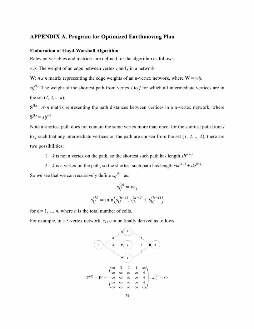
74

APPENDIX A. Program for Optimized Earthmoving Plan

Elaboration of Floyd-Warshall Algorithm

Relevant variables and matrices are defined for the algorithm as follows:

wij: The weight of an edge between vertex i and j in a network

W: n x n matrix representing the edge weights of an n-vertex network, where W = wij.

sij(k)

: The weight of the shortest path from vertex i to j for which all intermediate vertices are in

the set (1, 2,…,k).

S(k)

: n×n matrix representing the path distances between vertices in a n-vertex network, where

S(k)

= sij(k)

Note a shortest path does not contain the same vertex more than once; for the shortest path from i

to j such that any intermediate vertices on the path are chosen from the set (1, 2,…, k), there are

two possibilities:

1. k is not a vertex on the path, so the shortest such path has length sij(k-1)

2. k is a vertex on the path, so the shortest such path has length sik(k-1)

+skj(k-1)

So we see that we can recursively define sij(k)

as:

𝑠𝑖𝑗(0) 𝑖𝑗

𝑠𝑖𝑗(𝑘) min(𝑠𝑖𝑗

(𝑘−1), 𝑠𝑖𝑘(𝑘−1) + 𝑠𝑘𝑗

(𝑘−1))

for k = 1,…, n. where n is the total number of cells.

For example, in a 5-vertex network, s15 can be finally derived as follows:

𝑆(0) 𝑊

(

)

; 𝑠15

(0)

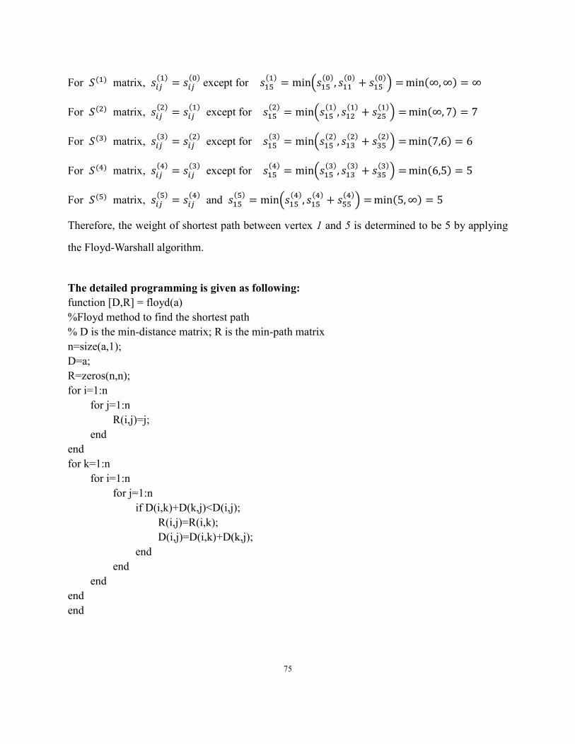
75

For 𝑆(1) matrix, 𝑠𝑖𝑗(1) 𝑠𝑖𝑗

(0) except for 𝑠15

(1) min(𝑠15

(0), 𝑠11(0)+ 𝑠15

(0)) min( , )

For 𝑆(2) matrix, 𝑠𝑖𝑗(2) 𝑠𝑖𝑗

(1) except for 𝑠15

(2) min(𝑠15(1), 𝑠12

(1) + 𝑠25(1)) min( , )

For 𝑆(3) matrix, 𝑠𝑖𝑗(3) 𝑠𝑖𝑗

(2) except for 𝑠15

(3) min(𝑠15(2), 𝑠13

(2) + 𝑠35(2)) min( , )

For 𝑆(4) matrix, 𝑠𝑖𝑗(4) 𝑠𝑖𝑗

(3) except for 𝑠15

(4) min(𝑠15(3), 𝑠13

(3) + 𝑠35(3)) min( , )

For 𝑆(5) matrix, 𝑠𝑖𝑗(5) 𝑠𝑖𝑗

(4) and 𝑠15

(5) min(𝑠15(4), 𝑠15

(4) + 𝑠55(4)) min( , )

Therefore, the weight of shortest path between vertex 1 and 5 is determined to be 5 by applying

the Floyd-Warshall algorithm.

The detailed programming is given as following:

function [D,R] = floyd(a) %Floyd method to find the shortest path % D is the min-distance matrix; R is the min-path matrix n=size(a,1); D=a; R=zeros(n,n); for i=1:n for j=1:n R(i,j)=j; end end for k=1:n for i=1:n for j=1:n if D(i,k)+D(k,j)<D(i,j); R(i,j)=R(i,k); D(i,j)=D(i,k)+D(k,j); end end end end end

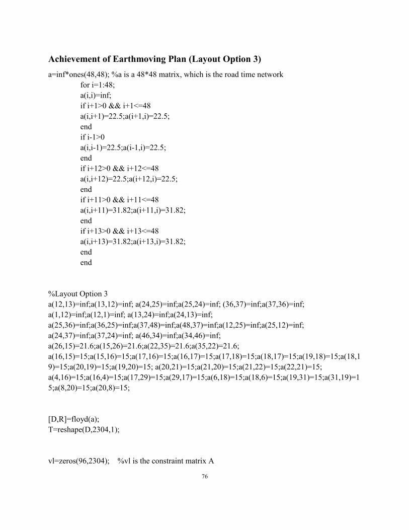
76

Achievement of Earthmoving Plan (Layout Option 3)

a=inf*ones(48,48); %a is a 48*48 matrix, which is the road time network for i=1:48; a(i,i)=inf; if i+1>0 && i+1<=48 a(i,i+1)=22.5;a(i+1,i)=22.5; end if i-1>0 a(i,i-1)=22.5;a(i-1,i)=22.5; end if i+12>0 && i+12<=48 a(i,i+12)=22.5;a(i+12,i)=22.5; end if i+11>0 && i+11<=48 a(i,i+11)=31.82;a(i+11,i)=31.82; end if i+13>0 && i+13<=48 a(i,i+13)=31.82;a(i+13,i)=31.82; end end

%Layout Option 3 a(12,13)=inf;a(13,12)=inf; a(24,25)=inf;a(25,24)=inf; (36,37)=inf;a(37,36)=inf; a(1,12)=inf;a(12,1)=inf; a(13,24)=inf;a(24,13)=inf;

a(25,36)=inf;a(36,25)=inf;a(37,48)=inf;a(48,37)=inf;a(12,25)=inf;a(25,12)=inf;

a(24,37)=inf;a(37,24)=inf; a(46,34)=inf;a(34,46)=inf;

a(26,15)=21.6;a(15,26)=21.6;a(22,35)=21.6;a(35,22)=21.6; a(16,15)=15;a(15,16)=15;a(17,16)=15;a(16,17)=15;a(17,18)=15;a(18,17)=15;a(19,18)=15;a(18,1

9)=15;a(20,19)=15;a(19,20)=15; a(20,21)=15;a(21,20)=15;a(21,22)=15;a(22,21)=15;

a(4,16)=15;a(16,4)=15;a(17,29)=15;a(29,17)=15;a(6,18)=15;a(18,6)=15;a(19,31)=15;a(31,19)=1

5;a(8,20)=15;a(20,8)=15;

[D,R]=floyd(a); T=reshape(D,2304,1);

vl=zeros(96,2304); %vl is the constraint matrix A

77

for j=1:48 for i=1:48 vl(j,(j-1)*48+i)=1; end end for j=1:48 for i=1:48 vl(48+j,(i-1)*48+j)=1; end end

ob=[15000,3700,0,0,0,0,1000,11200,2300,22000,6900,0,62600,0,0,0,0,0,0,24800,9900,2200,0,0,

3700,0,0,0,0,0,12400,34400,72500,28500,2500,0,0,1400,0,0,0,5900,9900,2700,0,0,0,0,0,0,3700,

9000,9000,8000,0,0,0,0,0,11200,0,22500,33800,36000,23000,22200,8100,0,0,0,14300,7900,0,22

500,28100,23000,24300,14200,0,0,0,0,0,0,0,0,2300,1200,9000,0,0,0,2200,0,0,0]; ob1=reshape(ob,96,1); %ob is the constaint matrix B ob1=ob

T1=T; lb=zeros(2304,1);ub=[];A=[];b=[];Aeq=vl;beq=ob1; [x,fval]=linprog(T1,A,b,Aeq,beq,lb); x=reshape(x,48,48) f=fval/(sum(ob)/2)

78

APPENDIX B. Program for Optimization of Temporary Haul Road Network

MCGA Functions

GA Initialize the Populations

function Chrom = GAInitPop( NIND,N ) %NIND is the size of each generation %N is the length of each gene Chrom=zeros(NIND,N); for i =1:NIND a=zeros(1,N); for i1=1:N if rand()<=0.5 a(i1)=0; else a(i1)=1; end end Chrom(i,:)=a; end a1=zeros(1,N); for i1=1:N a1(i1)=0; end a2=zeros(1,N); for i1=1:N a2(i1)=1; end Chrom(1,:)=a1; Chrom(NIND,:)=a2; end

GA EliteIndi

function [MinObjV,MinChrom] = GAEliteIndi( Chrom,ObjV,MinObjV,MinChrom ) %manual select MP=length(Chrom); for i=1:MP [Min0,minI]=min(ObjV{i}); if Min0<= MinObjV(i) && Min0~=0

79

MinObjV(i)=Min0; MinChrom(i,:)=Chrom{i}(minI,:); end end end

GA Fitness

function FitnV = GAFitness( ct,c) %ob1 is the objective function %fitness is 1./ob1 [a,b]=size(ct); FitnV=1./(1-48+ct); for i=1:a if ct(i)>c FitnV(i,1)=0; end end end

GA Immigrant

function [Chrom,ObjV] = GAimmigrant(Chrom,ObjV) %immigrant factor MP=length(Chrom); for i=1:MP if min(ObjV{i})~=0 [Min0,minI]=min(ObjV{i}); end next_i=i+1; if next_i>MP;next_i=mod(next_i,MP);end [Max0,maxI]=max(ObjV{next_i}); Chrom{next_i}(maxI,:)=Chrom{i}(minI,:); ObjV{next_i}(maxI)=ObjV{i}(minI); End

GA Intercross

function [ a,b ] = GAintercross( a,b ) %a&b are two individuls for intercross

80

L=length(a); r1=randsrc(1,1,[1:L]); r2=randsrc(1,1,[1:L]); if r1~=r2 a0=a;b0=b; s=min([r1,r2]); e=max([r1,r2]); for i=s:e a(i)=b0(i); b(i)=a0(i); end end end

GA Mutation

function SelCh = GAMutate( SelCh,Pm) %Pm is the possibility [NSel,L]=size(SelCh); for i=1:NSel if Pm>=rand R=randperm(L); SelCh(i,R(1:2))=SelCh(i,R(2:-1:1)); end end end

GA Recombine

function SelCh = GARecombin( SelCh,Pc ) %Pc is the intercross possibility NSel=size(SelCh,1); for i=1:2:NSel-mod(NSel,2) if Pc>=rand [SelCh(i,:),SelCh(i+1,:)]=GAintercross(SelCh(i,:),SelCh(i+1,:)); end end end

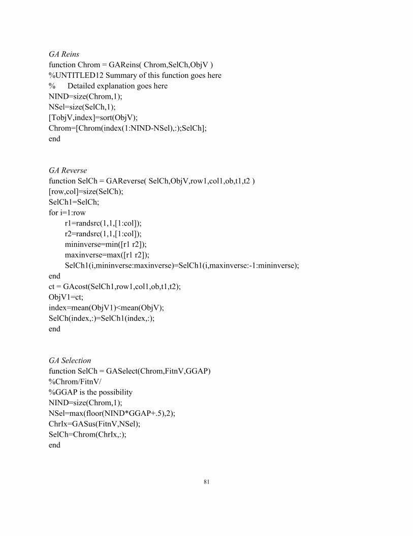
81

GA Reins

function Chrom = GAReins( Chrom,SelCh,ObjV ) %UNTITLED12 Summary of this function goes here % Detailed explanation goes here NIND=size(Chrom,1); NSel=size(SelCh,1); [TobjV,index]=sort(ObjV); Chrom=[Chrom(index(1:NIND-NSel),:);SelCh]; end

GA Reverse

function SelCh = GAReverse( SelCh,ObjV,row1,col1,ob,t1,t2 ) [row,col]=size(SelCh); SelCh1=SelCh; for i=1:row r1=randsrc(1,1,[1:col]); r2=randsrc(1,1,[1:col]); mininverse=min([r1 r2]); maxinverse=max([r1 r2]); SelCh1(i,mininverse:maxinverse)=SelCh1(i,maxinverse:-1:mininverse); end ct = GAcost(SelCh1,row1,col1,ob,t1,t2); ObjV1=ct; index=mean(ObjV1)<mean(ObjV); SelCh(index,:)=SelCh1(index,:); end

GA Selection

function SelCh = GASelect(Chrom,FitnV,GGAP) %Chrom/FitnV/ %GGAP is the possibility NIND=size(Chrom,1); NSel=max(floor(NIND*GGAP+.5),2); ChrIx=GASus(FitnV,NSel); SelCh=Chrom(ChrIx,:); end

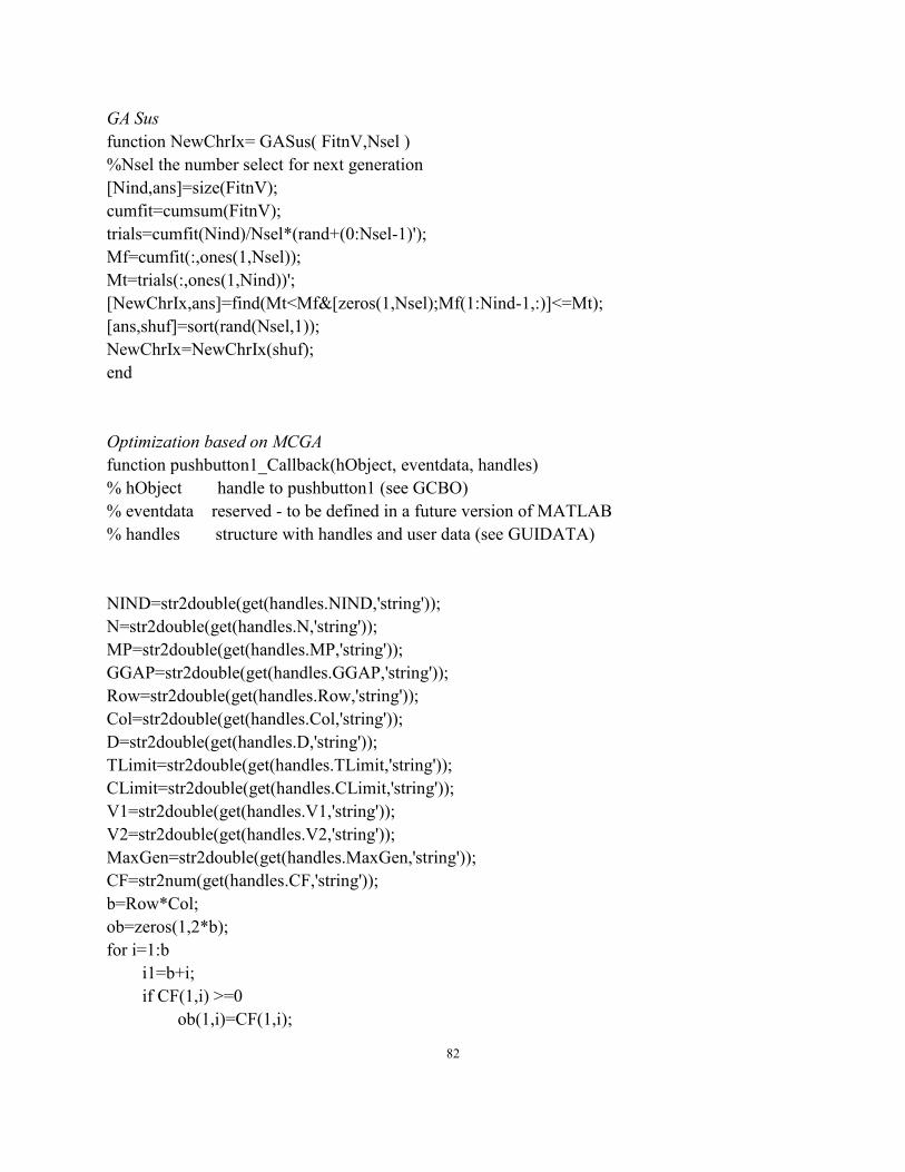
82

GA Sus

function NewChrIx= GASus( FitnV,Nsel ) %Nsel the number select for next generation [Nind,ans]=size(FitnV); cumfit=cumsum(FitnV); trials=cumfit(Nind)/Nsel*(rand+(0:Nsel-1)'); Mf=cumfit(:,ones(1,Nsel)); Mt=trials(:,ones(1,Nind))'; [NewChrIx,ans]=find(Mt<Mf&[zeros(1,Nsel);Mf(1:Nind-1,:)]<=Mt); [ans,shuf]=sort(rand(Nsel,1)); NewChrIx=NewChrIx(shuf); end

Optimization based on MCGA function pushbutton1_Callback(hObject, eventdata, handles) % hObject handle to pushbutton1 (see GCBO) % eventdata reserved - to be defined in a future version of MATLAB % handles structure with handles and user data (see GUIDATA)

NIND=str2double(get(handles.NIND,'string')); N=str2double(get(handles.N,'string')); MP=str2double(get(handles.MP,'string')); GGAP=str2double(get(handles.GGAP,'string')); Row=str2double(get(handles.Row,'string')); Col=str2double(get(handles.Col,'string')); D=str2double(get(handles.D,'string')); TLimit=str2double(get(handles.TLimit,'string')); CLimit=str2double(get(handles.CLimit,'string')); V1=str2double(get(handles.V1,'string')); V2=str2double(get(handles.V2,'string')); MaxGen=str2double(get(handles.MaxGen,'string')); CF=str2num(get(handles.CF,'string')); b=Row*Col; ob=zeros(1,2*b); for i=1:b i1=b+i; if CF(1,i) >=0 ob(1,i)=CF(1,i);

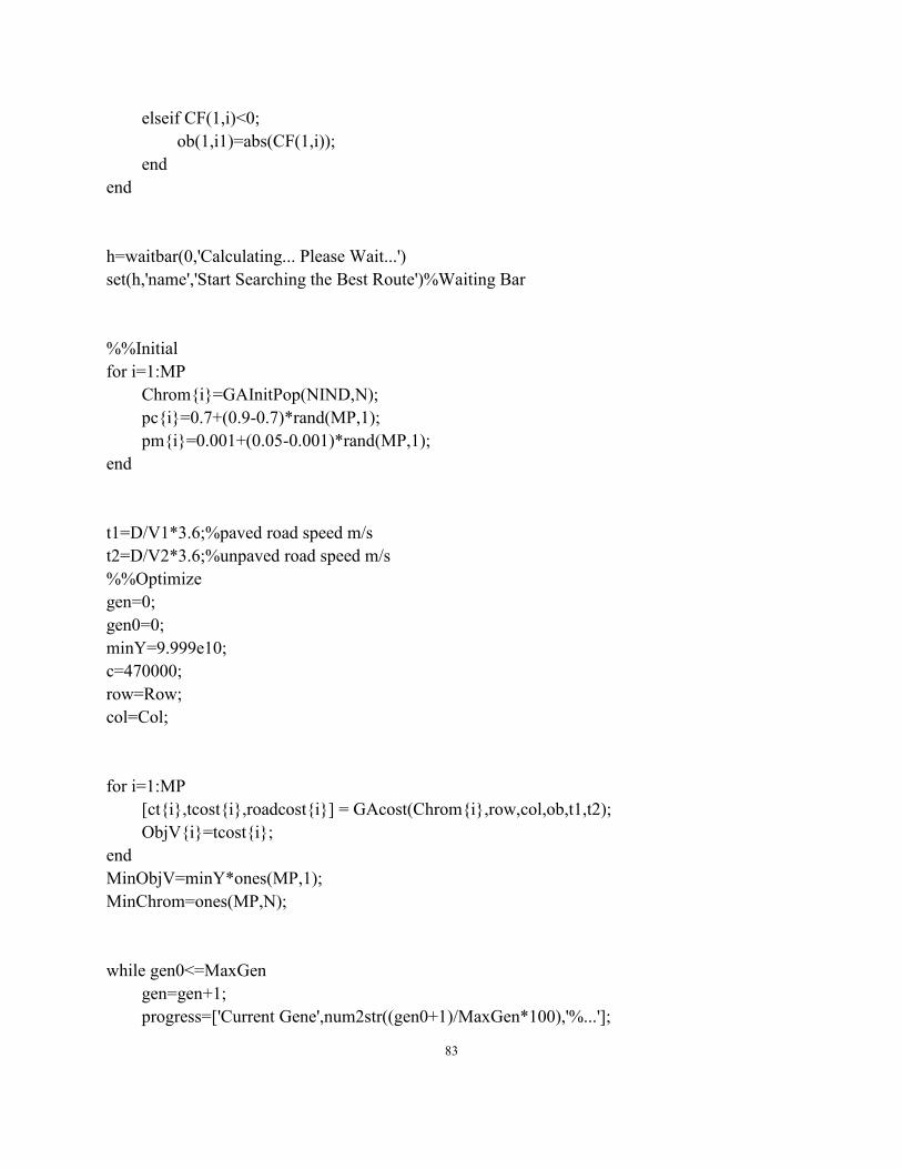
83

elseif CF(1,i)<0; ob(1,i1)=abs(CF(1,i)); end end

h=waitbar(0,'Calculating... Please Wait...') set(h,'name','Start Searching the Best Route')%Waiting Bar

%%Initial for i=1:MP Chrom{i}=GAInitPop(NIND,N); pc{i}=0.7+(0.9-0.7)*rand(MP,1); pm{i}=0.001+(0.05-0.001)*rand(MP,1); end

t1=D/V1*3.6;%paved road speed m/s t2=D/V2*3.6;%unpaved road speed m/s %%Optimize gen=0; gen0=0; minY=9.999e10; c=470000; row=Row; col=Col;

for i=1:MP [ct{i},tcost{i},roadcost{i}] = GAcost(Chrom{i},row,col,ob,t1,t2); ObjV{i}=tcost{i}; end MinObjV=minY*ones(MP,1); MinChrom=ones(MP,N);

while gen0<=MaxGen gen=gen+1; progress=['Current Gene',num2str((gen0+1)/MaxGen*100),'%...'];

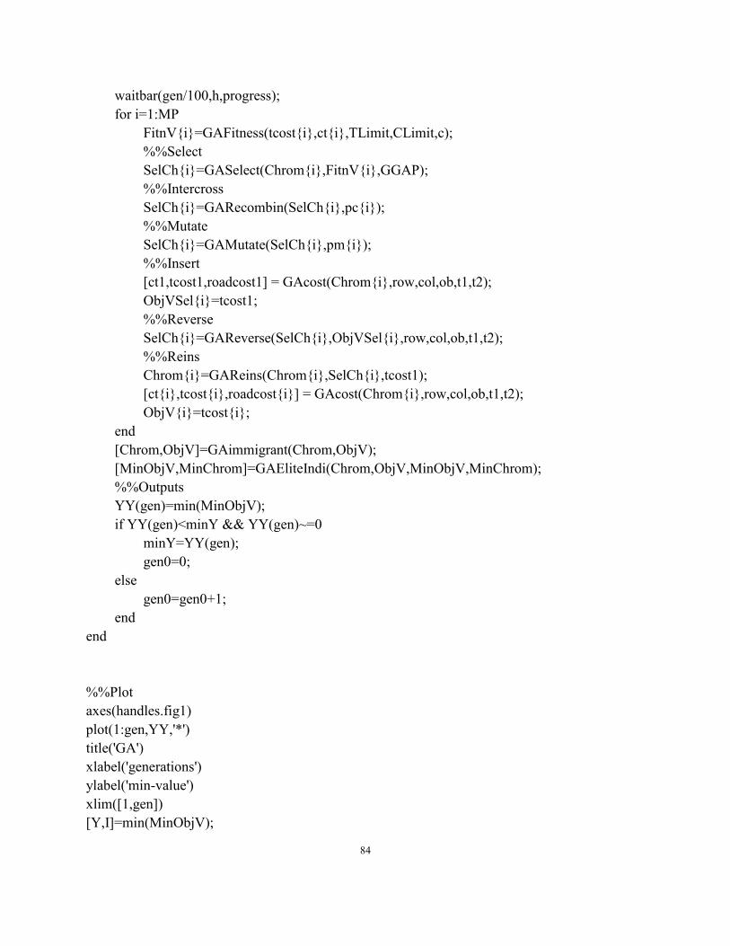
84

waitbar(gen/100,h,progress); for i=1:MP FitnV{i}=GAFitness(tcost{i},ct{i},TLimit,CLimit,c); %%Select SelCh{i}=GASelect(Chrom{i},FitnV{i},GGAP); %%Intercross SelCh{i}=GARecombin(SelCh{i},pc{i}); %%Mutate SelCh{i}=GAMutate(SelCh{i},pm{i}); %%Insert [ct1,tcost1,roadcost1] = GAcost(Chrom{i},row,col,ob,t1,t2); ObjVSel{i}=tcost1; %%Reverse SelCh{i}=GAReverse(SelCh{i},ObjVSel{i},row,col,ob,t1,t2); %%Reins Chrom{i}=GAReins(Chrom{i},SelCh{i},tcost1); [ct{i},tcost{i},roadcost{i}] = GAcost(Chrom{i},row,col,ob,t1,t2); ObjV{i}=tcost{i}; end [Chrom,ObjV]=GAimmigrant(Chrom,ObjV); [MinObjV,MinChrom]=GAEliteIndi(Chrom,ObjV,MinObjV,MinChrom); %%Outputs YY(gen)=min(MinObjV); if YY(gen)<minY && YY(gen)~=0 minY=YY(gen); gen0=0; else gen0=gen0+1; end end

%%Plot axes(handles.fig1) plot(1:gen,YY,'*') title('GA') xlabel('generations') ylabel('min-value') xlim([1,gen]) [Y,I]=min(MinObjV);

85

X=(MinChrom(I,:)); set(handles.opt,'string',num2str(Y)) set(handles.cb,'string',num2str(X))

%Try to plot the figure; a1=X; nod=row*col; a=inf*ones(nod,nod); %a is a 16*16 matrix, which is the road time network i1=1; for i=1:nod; a(i,i)=0; if i+1>0 && i+1<=nod && mod(i,row)~=0 a(i,i+1)=t2+a1(i1)*(t1-t2); a(i+1,i)=t2+a1(i1)*(t1-t2); i1=i1+1; end if i+row>0 && i+row<=nod a(i,i+row)=t2+a1(i1)*(t1-t2); a(i+row,i)=t2+a1(i1)*(t1-t2); i1=i1+1; end if i+row+1>0 && i+row+1<=nod && mod(i,row)~=0 a(i,i+row+1)=t2+a1(i1)*(1.414*t1-t2); a(i+row+1,i)=t2+a1(i1)*(1.414*t1-t2); i1=i1+1; end if i+row-1>0 && i+row-1<=nod && mod(i,row)~=0 && mod(i,row)~=1 a(i,i+row-1)=t2+a1(i1)*(1.414*t1-t2); a(i+row-1,i)=t2+a1(i1)*(1.414*t1-t2); i1=i1+1; end end

axes(handles.fig2) hold on box on for i=1:nod for j=1:nod

86

if a(i,j)~=0 && a(i,j)~=Inf && a(i,j)~=t2 y2=[(fix((i-1)/row))+1,(fix((j-1)/row))+1]; x2=[(mod(i-1,row))+1,(mod(j-1,row))+1]; plot(x2,y2,'-o','LineWidth',4) elseif a(i,j)~=0 && a(i,j)~=Inf && a(i,j)==t2 y2=[(fix((i-1)/row))+1,(fix((j-1)/row))+1]; x2=[(mod(i-1,row))+1,(mod(j-1,row))+1]; plot(x2,y2,'--o','LineWidth',1) end end end title('Optimized Network') xlabel('node') ylabel('node') xlim([1,row]) ylim([1,col]) close(h) msgbox('Finish Searching')