1

Optimization of Radar Parameters for Maximum DetectionProbability Under Generalized Discrete Clutter Conditions

Using Stochastic GeometryShobha Sundar Ram, Senior Member, IEEE, Gaurav Singh, and Gourab Ghatak, Member, IEEE

Abstract—We propose an analytical framework based on stochasticgeometry (SG) formulations to estimate a radar’s detection performanceunder generalized discrete clutter conditions. We model the spatialdistribution of discrete clutter scatterers as a homogeneous Poisson pointprocess and the radar cross-section of each extended scatterer as arandom variable of the Weibull distribution. Using this framework, wederive a metric called the radar detection coverage probability as afunction of radar parameters such as transmitted power, system noisetemperature and radar bandwidth; and clutter parameters such asclutter density and mean clutter cross-section. We derive the optimumradar bandwidth for maximizing this metric under noisy and clutteredconditions. We also derive the peak transmitted power beyond whichthere will be no discernible improvement in radar detection performancedue to clutter limited conditions. When both transmitted power andbandwidth are fixed, we show how the detection threshold can beoptimized for best performance. We experimentally validate the SGresults with a hybrid of Monte Carlo and full wave electromagnetic solverbased simulations using finite difference time domain (FDTD) techniques.

Index Terms—stochastic geometry, radar detection, FDTD, MonteCarlo simulations, indoor clutter, Poisson point process

I. INTRODUCTION

Clutter models serve as predictive tools for setting detectionthresholds and calibrating a radar’s performance during operation [1].Empirical models of clutter from land terrains, sea and precipitationhave been generated, over the decades, using large volumes ofhigh quality measurement data [2]–[4]. These data are typicallylaborious and time consuming to gather. Further, the computationof the statistical properties - such as higher order moments - fromthe data may be challenging [5], [6]. An alternate approach wouldbe to use computational tools to model clutter returns [7], [8]. Fullwave electromagnetic solvers are deterministic and computationallyexpensive especially at microwave and millimeter wave frequencies.Reliable characterization of radar detection metrics would requireextensive trials of full wave simulations to capture the stochasticnature of the target and clutter conditions. In particular, we needto consider multiple target and clutter deployments and, for eachof such realization, several clutter field-of-view and cross-sectioninstances must be considered. Moreover, this procedure would have tobe repeated for every set of possible radar parameters, e.g., bandwidthand center frequency. Therefore, such system level simulations arerarely used to quantify radar detection characteristics. In our paper,we propose the use of stochastic geometry (SG) to provide analyticalexpressions to quantitatively estimate a radar’s detection performance.

In recent years, SG has been explored for a variety of applica-tions [9]. For example, SG has been extensively studied in the contextof different types of communication systems including cellular net-works [10], [11], millimeter wave systems [12], [13], MIMO systems[14], [15], and vehicular networks [16]. The framework has beenexploited for optimizing communication parameters such as data rates

S.S.R., G. S and G. G are with the Indraprastha Institute of InformationTechnology Delhi, New Delhi 110020 India. E-mail: {shobha, gaurav18160,gourab.ghatak}@iiitd.ac.in.

under the given signal to interference ratio when multiple transmitters(such as base stations) and receivers (mobile end users) coexist inthe channel. Such an analytical characterization is especially usefulin capturing the diversity in the distribution and strength of the basestation signals in the region of interest.

More recently, SG-based analysis has been extended to radarscenarios [17]–[21]. In [17], [21], the authors modeled the distributionof the vehicles, mounted with automotive radars, on the roads asa Poisson point process, while in [18], [20], the distribution ofpulsed-radar sensors were modeled as a Poisson point process. Inall of the above works, SG techniques are used to characterizethe interference characteristics from multiple radars and analyticallyderive the signal to interference and noise ratio (SINR). The radardetection performance was then quantified on the basis of whetherthe SINR was above a pre-determined threshold. In this paper, wemodel the locations of discrete clutter scatterers as a Poisson pointprocess similar to [22]. Then, by employing tools from SG, wederive the signal to clutter and noise ratio (SCNR) in the region ofinterest. The radar detection performance is subsequently quantifiedbased on whether the SCNR exceeds a pre-determined threshold.Note that this formulation of the radar detection performance (andthose of the prior SG-based radar works) is fundamentally distinctfrom classical radar detection frameworks, such as the Neyman-Pearson approach, where likelihood ratio tests between alternative andnull hypotheses are performed to generate radar operating curves. Inclassical radar detection theory, the objective is usually to derive theprobability density functions (pdf) for signal plus noise and clutter(or interference) - the alternative hypothesis - and just noise andclutter (or interference) - the null hypothesis [23]. In contrast, ourSG-based radar work, characterizes the pdf of the SCNR directly.The main advantage is that SG-based analysis characterizes theradar performance for all possible spatial configurations of networkentities (in this case, discrete clutter scatterers) without the need forextensive simulations. Additionally, under suitable assumptions, suchan analysis leads to tractable analytical results which enables thederivation of system-design insights that are often missed by system-level simulations [24].

Two typical scenarios where discrete clutter are encountered areindoor radars [25] and foliage penetration radars [26]. Both theseradars typically operate at carrier frequencies below the X-bandin order to facilitate non-line-of-sight (NLOS) spotting of humans.Indoor radars encounter significant discrete clutter scatterers suchas furniture, walls, ceilings and floors [27]. Each of these discretescatterers consist of multiple scattering centers with significant aspectangle variation. Many different algorithms and strategies have beenproposed for mitigating both static and dynamic indoor clutter [28]–[31]. All of these studies focus on specific room layouts and wallgeometries. However, across different indoor environments, the scat-terers may show considerable variations in their spatial distributionsand sizes. Hence these radars may encounter considerable variationsin the clutter returns during actual deployments. Similarly, in foliagepenetration radar, returns from trees give rise to significant clutter

arX

iv:2

101.

1242

9v1

[ee

ss.S

P] 2

9 Ja

n 20

21

2

[26]. Again, there can be considerable spatial randomness in thetree’s girth and distribution. In both the cases, the radar performanceis based on the clutter characteristics such as its distribution, theradar cross-section (RCS) of each clutter scatterer as well as theinterference between the scatterers. Similarly, variations in the targetRCS and position can also affect the radar detection performance.The radar operating curves, in these scenarios, is directly a functionof the SCNR which is a random function of both target and clutterparameters. In our preliminary work in [32], we proposed a metrictermed as the radar detection coverage probability (PDC ) that ap-proximates the fraction of the locations of a target in the regionof interest where SCNR is above a predefined threshold. In thatpaper, we assumed an exponential distribution for the RCS of thediscrete clutter and derived PDC for both line-of-sight (LOS) andNLOS conditions of the target. Radar clutter have been modeled usingRayleigh, log-normal or Weibull distributions in prior works [33]–[35]. The log-normal model is typically used when the radar sees landclutter or sea clutter at low grazing angles, while the Rayleigh modelis used when the amplitude probability distribution of the clutter isof a limited dynamic range. However, both of these models providelimiting distributions for most experimentally measured clutter. TheWeibull model, on the other hand, provides a much more generalizedmodel for radar clutter and is adopted in this work to model thereturns from extended scatterers. We also assume that the noise, targetand clutter statistics do not change appreciably during the coherentprocessing interval of the radar. These conditions are generally metfor microwave or millimeter-wave radars. Our contributions in thispaper are summarised below:

1) We model discrete clutter scatterers as a homogeneous Poissonpoint process. We provide a comprehensive analysis of PDCunder generalized clutter conditions modeled using the Weibullfunction. Here, the exponential and Rayleigh clutter modelsare just two specific cases of the generalized Weibull cluttermodel. PDC also considers diversity in the RCS of the radartarget, the path loss function, the clutter density and themean RCS of the clutter scatterers. The theorems, we offer,provide physics based insights into the radar performance withrespect to different radar, target and clutter parameters insteadof laborious measurement experiments and computationallycomplex simulation studies.

2) The clutter returns that significantly affect the system per-formance arise from the same range cell occupied by thetarget. Greater bandwidth giving rise to small range cellsresult in weaker clutter returns. Noise, on the other hand,increases proportionately to bandwidth. We provide a tractablemethod for optimizing the radar bandwidth for maximizingthe radar detection coverage probability under discrete clutterand Gaussian noise conditions. The optimum radar bandwidth,derived from our theorem, will increase the likelihood of atarget being detected across the entire region of interest.

3) Under noise limited conditions, increase in transmitted powerresults in improved radar detection. However, in clutter limitedscenarios, there is no further improvement in the radar’s per-formance due to increased returns from the clutter scatterers.We provide an analytical solution for optimizing the radartransmitted power. When both the radar power and bandwidthare fixed, we provide a method to adjust the detection threshold.

4) Finally, all of the existing SG works have validated the resultsusing Monte Carlo simulations. In this work, we use a hybridof finite difference time domain (FDTD) techniques based onfull wave electromagnetic solvers and Monte Carlo simulationsto validate our SG results. To the best of our knowledge, our

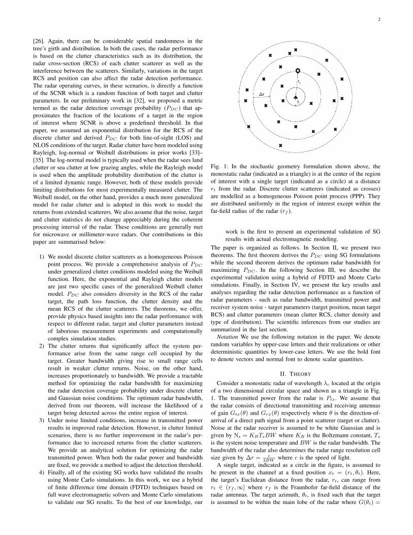
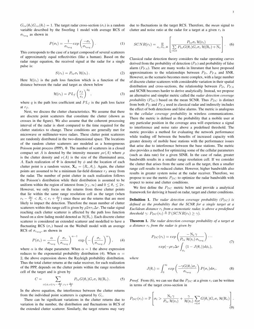
Fig. 1: In the stochastic geometry formulation shown above, themonostatic radar (indicated as a triangle) is at the center of the regionof interest with a single target (indicated as a circle) at a distancert from the radar. Discrete clutter scatterers (indicated as crosses)are modelled as a homogeneous Poisson point process (PPP). Theyare distributed uniformly in the region of interest except within thefar-field radius of the radar (rf ).

work is the first to present an experimental validation of SGresults with actual electromagnetic modeling.

The paper is organized as follows. In Section II, we present twotheorems. The first theorem derives the PDC using SG formulationswhile the second theorem derives the optimum radar bandwidth formaximizing PDC . In the following Section III, we describe theexperimental validation using a hybrid of FDTD and Monte Carlosimulations. Finally, in Section IV, we present the key results andanalyses regarding the radar detection performance as a function ofradar parameters - such as radar bandwidth, transmitted power andreceiver system noise - target parameters (target position, mean targetRCS) and clutter parameters (mean clutter RCS, clutter density andtype of distribution). The scientific inferences from our studies aresummarized in the last section.

Notation We use the following notation in the paper. We denoterandom variables by upper-case letters and their realizations or otherdeterministic quantities by lower-case letters. We use the bold fontto denote vectors and normal font to denote scalar quantities.

II. THEORY

Consider a monostatic radar of wavelength λc located at the originof a two dimensional circular space and shown as a triangle in Fig.1. The transmitted power from the radar is Ptx. We assume thatthe radar consists of directional transmitting and receiving antennasof gain Gtx(θ) and Grx(θ) respectively where θ is the direction-of-arrival of a direct path signal from a point scatterer (target or clutter).Noise at the radar receiver is assumed to be white Gaussian and isgiven by Ns = KBTsBW where KB is the Boltzmann constant, Tsis the system noise temperature and BW is the radar bandwidth. Thebandwidth of the radar also determines the radar range resolution cellsize given by ∆r = c

2BWwhere c is the speed of light.

A single target, indicated as a circle in the figure, is assumed tobe present in the channel at a fixed position xt = (rt, θt). Here,the target’s Euclidean distance from the radar, rt, can range fromrt ∈ (rf ,∞] where rf is the Fraunhofer far-field distance of theradar antennas. The target azimuth, θt, is fixed such that the targetis assumed to be within the main lobe of the radar where G(θt) =

3

Gtx(θt)Grx(θt) = 1. The target radar cross-section (σt) is a randomvariable described by the Swerling 1 model with average RCS ofσtavg as shown in

P (σt) =1

σtavg

exp

(−σtσtavg

). (1)

This corresponds to the case of a target composed of several scatterersof approximately equal reflectivities (like a human). Based on theradar range equation, the received signal at the radar for a singlepulse is:

S(rt) = PtxσtH(rt) . (2)

Here H(rt) is the path loss function which is a function of thedistance between the radar and target as shown below

H(rt) = PLf

(rfrt

)2q

, (3)

where q is the path loss coefficient and PLf is the path loss factorat rf .

Next, we discuss the clutter characteristics. We assume that thereare discrete point scatterers that constitute the clutter (shown ascrosses in the figure). We also assume that the coherent processinginterval of the radar is short compared to the time required for theclutter statistics to change. These conditions are generally met formicrowave or millimeter-wave radars. These clutter point scatterersare randomly distributed in the two-dimensional space. The locationsof the random clutter scatterers are modeled as a homogeneousPoisson point process (PPP), Φ. The number of scatterers in a closedcompact set A is denoted by the intensity measure ρν(A) where ρis the clutter density and ν(A) is the size of the illuminated area,A. Each realization of Φ is denoted by φ and the location of eachclutter point is a random vector, Xc = (Rc, θc). Again, the clutterpoints are assumed to be a minimum far-field distance rf away fromthe radar. The number of point clutter in each realization followsthe Poisson’s distribution while their distribution is assumed to beuniform within the region of interest from [rf ,∞) and 0 ≤ θc ≤ 2π.However, we only focus on the returns from those clutter pointsthat lie within the same range resolution cell as the target (whenrt − ∆r

2< Rc < rt + ∆r

2) since these are the returns that are most

likely to impact the detection. Therefore the mean number of clutterscatterers within this range cell is given by ρ2πrt∆r. The radar signalreaching each clutter scatterer is affected by the path loss functionbased on a slow fading model denoted asH(Rc). Each discrete clutterscatterer is considered an extended scatterer and modelled to have afluctuating RCS (σc) based on the Weibull model with an averageRCS of σcavg , as shown in

P (σc) =α

σcavg

(σcσcavg

)α−1

exp

(−(

σcσcavg

)α), (4)

where α is the shape parameter. When α = 1 the above expressionreduces to the exponential probability distribution (4). When α =2, the above expression shows the Rayleigh probability distribution.Thus the total clutter returns at the radar receiver, for each realizationof the PPP, depends on the clutter points within the range resolutioncell of the target and is given by

C =∑

c∈φ,c∈rt−∆r2,rt+ ∆r

2

PtxG(θc)GcσcH(Rc) . (5)

In the above equation, the interference between the clutter returnsfrom the individual point scatterers is captured by Gc.

There can be significant variations in the clutter returns due tovariation in the number, the distribution and fluctuations in RCS ofthe extended clutter scatterer. Similarly, the target returns may vary

due to fluctuations in the target RCS. Therefore, the mean signal toclutter and noise ratio at the radar for a target at a given rt is

SCNR(rt) = Eσc,Gc,Φ

PtxσtH(rt)∑c∈φ

PtxG(θc)GcσcH(Rc) + Ns

. (6)

Classical radar detection theory considers the radar operating curvesderived from the probability of detection (PD) and probability of falsealarm (PFA). There are many works in literature that have proposedapproximations to the relationships between PD , PFA and SNR.However, as the scenario becomes more complex, with a large numberof discrete clutter scatterers with considerable variation in their spatialdistribution and cross-sections, the relationship between PD , PFAand SCNR becomes harder to derive analytically. Instead, we proposean alternative and simpler metric called the radar detection coverageprobability (PDC ) based on the mean SCNR. Thus PDC is distinctfrom both PD and PFA used in classical radar and indirectly includesthe effect of both detections and false alarms. The metric is analogousto the cellular coverage probability in wireless communications.There the metric is defined as the probability that a mobile user atany particular position in the coverage area will experience a signalto interference and noise ratio above a predefined threshold. Themetric provides a method for evaluating the network performancewhile trading off between the benefits of increased capacity withgreater density of mobile base stations with the performance issuesthat arise due to interference between the base stations. The metricalso provides a method for optimizing some of the cellular parameters(such as data rate) for a given SINR. In the case of radar, greaterbandwidth results in a smaller range resolution cell. If we considerthe clutter that arises from the same cell as the target, then a smallerrange cell results in reduced clutter. However, higher bandwidth alsoresults in greater system noise at the radar receiver. Therefore, wepropose to use the metric PDC to optimize the radar bandwidth withrespect to noise and clutter conditions.

We first define the PDC metric below and provide a analyticalframework for deriving it based on radar, target and clutter conditions.

Definition 1. The radar detection coverage probability (PDC ) isdefined as the probability that the SCNR for a single target at aEuclidean distance rt from a monostatic radar, is above a predefinedthreshold γ: PDC(rt) , P (SCNR(rt) ≥ γ).

Theorem 1. The radar detection coverage probability of a target ata distance rt from the radar is given by

PDC(rt) = exp

(−Ns γ

PtxH(rt)σtavg

)· · ·

exp(−ρrt∆r∫φc

(1− J(θc))dφc),

(7)

where

J(θc) =

∫ ∞0

exp

(−γG(θc)σc

σtavg

)P (σc)dσc. (8)

Proof. From (6), we can see that the PDC at a given rt can be writtenin terms of the target cross-section in

PDC(rt) = P

σt > Ns γ

PtxH(rt)+

γ

H(rt)

∑c∈φ

G(θc)GcσcH(Rc)

.(9)

4

Due to the exponential distribution of the target RCS in (1), the aboveexpression becomes

Eσc,Gc,Φ

exp −Ns γ

PtxH(rt)σtavg

+∑c∈φ

−γG(θc)GcσcH(Rc)

H(rt)σtavg

= exp

(−Ns γ

PtxH(rt)σtavg

)I(·)

(10)

In the above expression, the terms within the first exponent - Ns, γPtx, H(rt) and σtavg - are all deterministic. This term encompassesthe signal-to-noise (SNR) ratio with respect to the target returns.The second exponential term, I(·) shows the stochasticity of theclutter conditions (clutter cross-section and the PPP distribution ofthe clutter points). This term is independent of Ptx and is a functionof the signal-to-clutter ratio (SCR) of the system. I(·) can be furtherevaluated as

I(·) = Eσc,Gc,Φ

[∏c∈Φ

exp

(−γG(θc)GcσcH(Rc)

H(rt)σtavg

)], (11)

since the exponential of sum terms can be written as the productof exponential terms. Using the probability generating functional(PGFL) of SG [36], we obtain

I(·) = exp(−ρ∫ rt+ ∆r

2

rt−∆r2

∫ 2π

0

(1− · · ·

Eσc,Gc

[exp

(−γG(θc)GcσcH(rc)

H(rt)σtavg

)])d(~xc))

= exp

(−ρ∫ rt+ ∆r

2

rt−∆r2

∫ 2π

0

(1− J(·)) rcdφcdrc

) (12)

As pointed out before, we only consider the discrete clutter that arisewithin the same range cell as the target. The inner expectation term,J(·), depends on the distribution of σc and the interference term Gc.Under worst case scenarios, Gc is always 1 and the clutter returnsadd. Then

J(·) = Eσc

[exp

(−γG(θc)σcH(rc)

H(rt)σtavg

)]=

∫ ∞0

exp

(−γG(θc)σcH(rc)

H(rt)σtavg

)P (σc)dσc

(13)

Now if the range resolution cell is sufficiently narrow, which isusually the case for microwave and millimeter wave radars, thenH(rc) ∼ H(rt) when rt − ∆r

2≤ rc ≤ rt + ∆r

2. Therefore (13)

becomes independent of rt as shown below in

J(θc) =

∫ ∞0

exp

(−γG(θc)σc

σtavg

)P (σc)dσc. (14)

Substituting this in (12), we obtain

I = exp(−ρrt∆r∫φc

(1− J(θc))dφc). (15)

Combining (13), (11) and (10), we prove the theorem.

In the above discussion not all distributions lead to tractablesolutions. For example, the choice of exponential model (Swerling1/2) model of the target RCS was crucial. The higher order Swerling3 distribution results in far more challenging mathematical operationsand hence not discussed here. In [32], we discussed the effect of thegain of the radar antennas on the detection performance. We do notrepeat that discussion here and confine our discussion to isotropicradar antennas where G(θc) = 1. The J(·) term which is a functionof the clutter cross-section can be computed numerically. However

for two cases, when α = 1 corresponding to exponential distributionand for α = 2 corresponding to Rayleigh distribution, analyticalexpressions for J(·) are derived.

Case 1: When α = 1 for exponential distribution of clutter, withmean clutter cross-section, σcavg , the J(·) term reduces to

J =1

1 + ν(16)

where ν =γ σcavg

σtavg. Substituting this expression back in (11), we

obtain

I = exp

(−2πρ

ν

ν + 1rt∆r

)(17)

which can be easily evaluated numerically.Case 2: When α = 2 for Rayleigh distribution of clutter, the

analytical solution for J is

J = 1−√πν

2eν

2/4erf(ν

2), (18)

where erf(·) is the error function. This results in

I = exp(−π1.5ρνeν

2/4erf(ν

2)rt∆r

)(19)

Corollary 1.1. In case 1, when ν is much greater than 1 whichcorresponds to the situation when σcavg � σtavg , then I becomesindependent of ν. As a result, PDC becomes independent of σcavg .Similarly, in case 2, the exponential term (eν

2/4) within J becomesvery high when ν is high. As a result I converges to 1 and the PDCis no longer a function of σcavg . In other words. PDC deteriorateswith increase in σcavg till it asymptotically converges at a limit.

Corollary 1.2. The same effect of PDC versus σcavg is observedfor generalized Weibull clutter parameter α. If we define κ =−γG(θc)H(rc)

H(rt)in the generalized J in (13), then the first derivative

of J with respect to σcavg is given by

dJ

d σcavg

=

∫ ∞0

exp(−κσc) · · ·[ασα−1

c

σcavgαexp

(−(

σcσcavg

)α)( −ασcavg

α+1− α

(σcσcavg

)α−1)]

.

(20)

In (20), the terms inside the integral are always negative. Since J isbounded below and a decreasing function of σcavg , we can concludethat as σcavg tends to ∞, J will tend to 0. Hence, for high values ofσcavg , PDC is independent of σcavg for generalized Weibull clutterconditions.

Corollary 1.3. In (7), it is evident that the first exponential termindicates the effect of the SNR on the radar detection performancewhile the second term shows the effect of SCR. Hence increase in thetransmitted power improves the radar detection performance whilethe radar operates in the noise limited scenario but has limitedimpact on the performance when the radar enters the clutter limitedscenario. For fixed target and clutter conditions, PDC converges toIconv with increase in Ptx. The transmitted power at which detectionperformance reaches 99% (e−0.01) of the convergence value is givenby

Iconve−0.01 = exp

(−Ns γ

Pmaxtx H(rt)σtavg

)Iconv

=> Pmaxtx =100 Ns γ

H(rt)σtavg

(21)

The maximum transmitted power is therefore independent of clutterparameters such as ρ, σcavg and α.

5

Corollary 1.4. In the above discussion, the radar detection coverageprobability is provided in terms of the clutter density, ρ. However, insome experiments, other spatial statistical parameters besides clutterdensity may be used. One popular parameter is the average nearestneighbor distance, r, which is the average distance between thecentroid of a clutter point and its nearest neighboring clutter point.For a uniform random distribution of the clutter points, the averagenearest neighbor distance is related to the clutter density [37] asshown below

r =1

2√ρ

(22)

Therefore, the radar detection probability in (7) can be written as

PDC(rt) = exp

(−Ns γ

PtxH(rt)σtavg

)· · ·

exp

(−rt∆r

2r2

∫φc

(1− J(θc))dφc

) (23)

When the distribution of the clutter points deviate from the uniformdistribution and cluster in some regions, the inhomogenity of theclutter distribution can be modeled either with the a non-uniformclutter density (ρ(xc)) or through additional statistics on the averagenearest neighbor distance [37].

Next, we provide a theorem for optimizing the radar BW undernoisy and cluttered conditions.

Theorem 2. For a narrow range resolution cell, the optimum BWfor detecting a Swerling 1 target is given by

BW =

√πρc(1− J)rtPtxH(rt)σtavg

KBTsγ. (24)

Proof. For a narrow ∆r and isotropic radar antennas, the integral in(15) can be reduced to

I(·) = exp (−2πρ(1− J)rt∆r) (25)

Therefore the radar detection probability is a function of BW asshown in

PDC = exp

(−KBTsBWγ

PtxH(rt)σtavg

)exp

(−2πρ(1− J)rt

c

2BW

).

(26)

Higher BW results in greater noise which causes a reduction in thePDC due to the first exponential term. However increase in BWalso results in a reduced ∆r resulting in lesser clutter returns as seenin the second exponential term. Therefore, the optimum BW formaximizing PDC can be determined by taking a natural logarithmon both sides of (26) as shown below

lnPDC =−KBTsBWγ

PtxH(rt)σtavg

− 2πρ(1− J)rtc

2BW. (27)

The optimum BW , shown in (24), is obtained when the firstderivative of the above expression with respect to BW is equatedto zero.

The optimum BW is shown to be a function of the target distancefrom the radar. In many situations it may not possible to changethe radar bandwidth while tracking the target. In those scenarios, itmay be preferable to be able to adjust the threshold γ for a fixedtransmitted power and radar bandwidth BW .

Corollary 2.1. The γ for obtaining the maximum PDC for a givenradar transmitted power and bandwidth for large clutter cross-sections should be adjusted based on the target distance rt using

γ(rt) =πρcrtPtxH(rt)σtavg

KBTsBW 2. (28)

We have already observed from corollaries 1.1 and 1.2 that Jbecomes 0 for high σcavg . Therefore, in those scenarios, the aboveexpression is directly obtained from (24). Note that in the aboveexpression, the γ is independent of the type of clutter cross-sectiondistribution (α) and is only dependent on the density of the clutterscatterers.

III. EXPERIMENTAL VALIDATION

In prior works, the experimental validation of the SG resultswere based on Monte Carlo simulations. However, the completeelectromagnetic phenomenology (attenuation, diffraction, scattering)are not captured through these simulations. Therefore, in this paper,we use a full wave electromagnetic solver to model the complete radarpropagation phenomenology. However, the computational complexityof these solvers is dependent on the size of the region of interestand the wavelength of the source excitation. Also, these solversare inherently deterministic and cannot capture the diversity inradar, target and clutter parameters. Therefore, we use a hybrid ofelectromagnetic based modeling based on finite FDTD and MonteCarlo based simulations to experimentally validate the SG results.

A. Finite Difference Time Domain Simulations

The FDTD technique models the complete propagation physicsbetween a source and the scatterers in a medium. Many priorworks have used FDTD for modeling indoor clutter [31], [38]–[42].For computational simplicity, we consider a two-dimensional (2D)simulation space along the XY plane spanning 20m by 20m. Anarrowband sinusoidal infinitely long, line source at 1 GHz emulatingthe monostatic radar is introduced at the center of the space at (0, 0)m.The space is discretized into grid points that are uniformly spacedλc10

apart where λc is the wavelength corresponding to the sourceexcitation. The entire simulation space is bounded by a perfectlymatched layer (PML) of 2λc thickness.

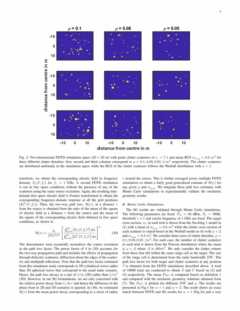
The distribution of discrete clutter scatterers in the FDTD spacefollows the homogeneous PPP. For a given clutter density ρ, weperform multiple FDTD simulations as shown in Fig.2. Each columnin the figure shows three FDTD simulations for a specific ρ. Thenumber of scatterers in a FDTD realization follows the Poissondistribution where the mean number of scatterers across multipleFDTD simulations is ρ × A where A = 400 m2 is the area ofthe simulation space. In each FDTD simulation, the scatterers aredistributed uniformly about the simulation space except within aradius of rf = 3m around the source. Each scatterer is modelled asan infinitely long dielectric cylinder of dielectric constant εr = 7.1and radius rg . The RCS, σc, of each of the clutter scatterers is arandom variable drawn from the Weibull distribution of mean cross-section, σcavg = 0.8m2 and shape parameter α = 1 (or 2) as given in(4). Using modal analysis, the 2D RCS of an infinitely long cylinderis given in terms of Bessel and Hankel functions as shown in

σc =16

k

[−J0(krg)

H10(krg)

+

N∑n=1

2(−1)n+1 Jn(krg)

H1n(krg)

]2

, (29)

where k = 2π√εr/λ and N is the number of modes [43]. The unit

of the 2D RCS is in meters rather than square-meters (3D). Basedon the above equation, a look up table is formed between rg and σcusing a sufficiently large value of N (50, in our case) when σc hasconverged. Using this look up table, rg is estimated for each σc ofthe scatterer. We further approximate the cylinders to have a squareshaped longitudinal cross-section for simplicity.

The FDTD models the time-domain transverse electric field,Ez(~r, t), in the two-dimensional grid space (~r). Through Fourier

6

Fig. 2: Two-dimensional FDTD simulation space (20× 20 m) with point clutter scatterers of εr = 7.1 and mean RCS σcavg = 0.8 m2 forthree different clutter densities: first, second and third columns correspond to ρ = 0.1, 0.08, 0.05 1/m2 respectively. The clutter scatterersare distributed uniformly in the simulation space while the RCS of the clutter scatterers follows the Weibull distribution with α = 1.

transform, we obtain the corresponding electric field in frequencydomain, Ez(~r, fc) for fc = 1 GHz. A second FDTD simulationis run in free space conditions without the presence of any of thescatterers using the same source excitation. Again, the resulting time-domain free space electric field is Fourier transformed to obtain thecorresponding frequency-domain response at all the grid positions(Efsz (~r, fc)). Then, the two-way path loss, H(r), at a distance rfrom the source is obtained from the ratio of the mean of the squareof electric field at a distance r from the source and the mean ofthe square of the corresponding electric field obtained in free spaceconditions, as shown in

H(r) =λc

(2π)3r2

∮ 2π

φ=0

∣∣Ez(~r, fc)2∣∣ dφ∮ 2π

φ=0

∣∣∣Efsz (~r, fc)2

∣∣∣ dφ2

. (30)

The denominator term essentially normalizes the source excitationin the path loss factor. The power factor of 4 in (30) accounts forthe two-way propagation path and includes the effects of propagationthrough dielectric scatterers, diffraction about the edges of the scatter-ers and multipath reflections. Note that the path loss factor estimatedfrom this simulation study corresponds to 2D cylindrical waves ratherthan 3D spherical waves that correspond to the usual radar scenario.Hence, the path loss decays at a rate of 1/m (2D) rather than 1/m2

(3D). However, in our SG formulations, we are only concerned withthe relative power decay from rf to r and hence the difference in thephase front in 2D and 3D scenarios is ignored. In (30), we estimatedH(r) from the mean power decay corresponding to a circle of radius

r around the source. This is further averaged across multiple FDTDsimulations to obtain a fairly good generalized estimate of H(r) forany given ρ and σcavg . We integrate these path loss estimates withMonte Carlo simulations to experimentally validate the stochasticgeometry results.

B. Monte Carlo Simulations

The SG results are validated through Monte Carlo simulations.The following parameters are fixed: Ptx = 30 dBm, Ns = 300K,threshold γ = 1 and carrier frequency of 1 GHz are fixed. The targetcross-section, σt, in each trial is drawn from the Swerling 1 model in(1) with a mean of σtavg = 0.8 m2 while the clutter cross-section ofeach scatterer is varied based on the Weibull model in (4) with α = 2and σcavg = 0.8 m2. We consider three cases of clutter densities: ρ =0.1, 0.08, 0.05 /m2. For each case, the number of clutter scatterersin each trial is drawn from the Poisson distribution where the meanis ρ × A where A is 400m2. We only consider the clutter returnsfrom those that fall within the same range cell as the target. The sizeof the range cell is determined from the radar bandwidth BW . Thepath loss factor for both target and clutter scatterers at any position~r is obtained from the FDTD simulations described above. A totalof 10000 trials are conducted to obtain S and C based on (2) and(5) respectively. The mean PDC is computed based on definition 1and compared with the stochastic geometry solutions obtained from(7). The PDC is plotted for different BW and ρ. The results arepresented in Fig.3 for α = 1 and α = 2. The result shows an exactmatch between FDTD and SG results for α = 1 (Fig.3a) and a very

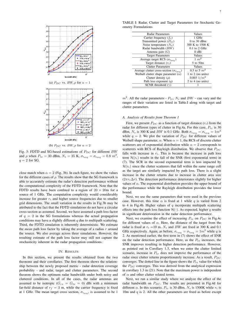
7

(a) PDC vs. BW, ρ for α = 1

(b) PDC vs. BW, ρ for α = 2

Fig. 3: FDTD and SG-based estimations of PDC for different BWand ρ when Ptx = 30 dBm, Ns = 35 K, σtavg = σcavg = 0.8 m2,q = 2 for SG.

close match when α = 2 (Fig. 3b). In each figure, we show the valuesfor the different cases of ρ. The results show that the SG framework isable to accurately estimate the radar’s detection performance withoutthe computational complexity of the FDTD framework. Note that theFDTD results have been confined to a region of 20 × 20m for asource of 1 GHz. The computation complexity would considerablyincrease for greater rt and higher source frequencies due to smallergrid dimensions. The small variation in the results in Fig.3b may beattributed to the fact that the FDTD simulations do not have a circularcross-section as assumed. Second, we have assumed a path loss factorof q = 2 in the SG formulations whereas the actual propagationconditions may have a slightly different q due to multipath scattering.Third, the FDTD simulation is inherently deterministic. We estimatethe mean path loss factor by taking the average of a radius r aroundthe source. We also average across three simulations. However, theresulting estimate of the path loss factor may still not capture thestochasticity inherent in the radar propagation conditions.

IV. RESULTS

In this section, we present the results obtained from the twotheorems and their corollaries. The first theorem shows the relation-ship between the newly proposed metric - radar detection coverageprobability - and radar, target and clutter parameters. The secondtheorem shows the optimum radar bandwidth under both noisy andcluttered conditions. In all of the cases, the radar antennas areassumed to be isotropic (Grx = Gtx = 0) dBi with a minimumfar-field distance of rf = 3 m, while the carrier frequency is fixedat 1 GHz. The mean target cross section, σtavg , is assumed to be 1

TABLE I: Radar, Clutter and Target Parameters for Stochastic Ge-ometry Formulations

Radar Parameters ValuesCarrier frequency (fc) 1 GHz

Transmitted power (Ptx) 0 to 30 dBmNoise temperature (Ns) 300 K to 1500 KRadar bandwidth (BW ) 0.1 to 2 GHz

Antenna gain (G) 0 dBiTarget Parameters Values

Average target RCS (σtavg ) 1 m2

Target distance (rt) 5 to 50mClutter Parameters Values

Average clutter cross-section (σcavg ) 0.5 to 5 m2

Weibull clutter shape parameter (α) 1 to 2 (no units)Clutter density (ρ) 0.003 1/m2

Path loss exponent (q) 2 to 4 (no units)SCNR threshold (γ) 1

m2. All the radar parameters - Ptx, Ns and BW - can vary and theranges of their variation are listed in Table.I along with target andclutter parameters.

A. Analysis of Results from Theorem 1

First, we present PDC as a function of target distance (rt) from theradar for different types of clutter in Fig.4a. For this case, Ptx is 30dBm, Ns is 300 K and BW is 0.1 GHz. Both σcavg = σtavg = 1m2

while q = 2. We plot the variation of PDC for different values ofWeibull shape parameter, α. When α = 1, the RCS of discrete clutterscatterers are of exponential distribution while α = 2 corresponds toscatterers with RCS of Rayleigh distribution. We observe that PDCfalls with increase in rt. This is because the increase in path lossterm H(rt) results in the fall of the SNR (first exponential term) in(7). The SCR in the second exponential term is less impacted byH(rt) since the clutter scatterers that fall within the same range cellas the target are similarly impacted by path loss. There is a slightincrease in the clutter returns due to increase in clutter area size(2πrt∆r). The detection performance deteriorates slightly for highervalues of α. The exponential distribution provides the upper bound ofthe performance while the Rayleigh distribution provides the lowerbound.

Next, we use the same parameters that were used in the previouscase. However, this time α is fixed at 1 while q is varied from 2to 4 in Fig.4b. Higher values of q incorporate multipath scatteringeffects into the path loss function H(·). As expected, higher q resultsin significant deterioration in the radar detection performance.

Next, we examine the effect of increasing Ptx on PDC in Fig.4cfor different values of α. Here, the distance of the target from theradar is fixed at rt =10 m. Ns and BW are fixed at 300 K and 0.1GHz respectively. Again, as before, σcavg = σtavg = 1m2 while q is2. As mentioned earlier, the first term in (7) shows the effect of SNRon the radar detection performance. Here, as the Ptx increases, theSNR improves resulting in higher detection performance. However,as pointed out in Corollary 1.3, when we enter the clutter limitedscenario, increase in Ptx does not improve the performance of theradar since clutter returns proportionately increase. As a result, PDCconverges. The dotted line in the figure shows the Ptx value for whichthe PDC converges. This was derived from the analytical expressionin corollary 1.3 in (21). Note that the maximum power is independentof α and other clutter related terms.

Next, we run a similar study where we analyze the effect of theradar bandwidth on PDC . The results are presented in Fig.4d fordifferent α. In this scenario, Ptx is 30 dBm, Ns is 1500K while rt is10m and q is 2. All the other parameters are fixed as before except

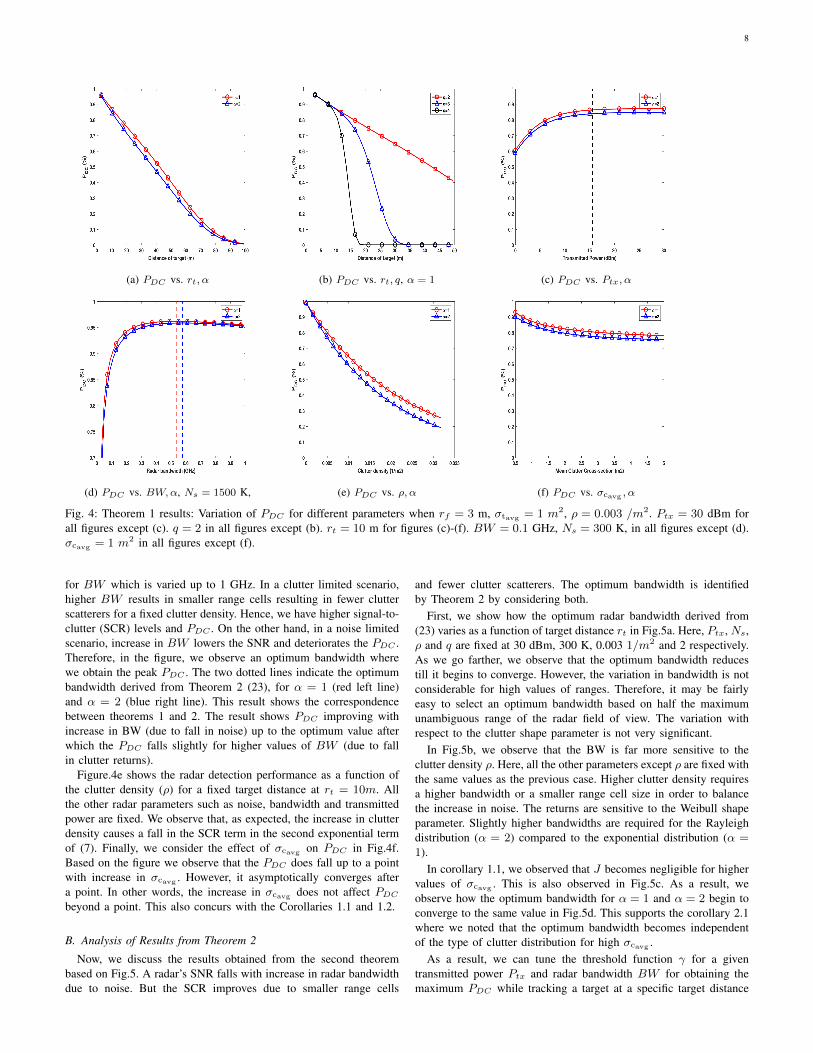
8

(a) PDC vs. rt, α (b) PDC vs. rt, q, α = 1 (c) PDC vs. Ptx, α

(d) PDC vs. BW,α, Ns = 1500 K, (e) PDC vs. ρ, α (f) PDC vs. σcavg , α

Fig. 4: Theorem 1 results: Variation of PDC for different parameters when rf = 3 m, σtavg = 1 m2, ρ = 0.003 /m2. Ptx = 30 dBm forall figures except (c). q = 2 in all figures except (b). rt = 10 m for figures (c)-(f). BW = 0.1 GHz, Ns = 300 K, in all figures except (d).σcavg = 1 m2 in all figures except (f).

for BW which is varied up to 1 GHz. In a clutter limited scenario,higher BW results in smaller range cells resulting in fewer clutterscatterers for a fixed clutter density. Hence, we have higher signal-to-clutter (SCR) levels and PDC . On the other hand, in a noise limitedscenario, increase in BW lowers the SNR and deteriorates the PDC .Therefore, in the figure, we observe an optimum bandwidth wherewe obtain the peak PDC . The two dotted lines indicate the optimumbandwidth derived from Theorem 2 (23), for α = 1 (red left line)and α = 2 (blue right line). This result shows the correspondencebetween theorems 1 and 2. The result shows PDC improving withincrease in BW (due to fall in noise) up to the optimum value afterwhich the PDC falls slightly for higher values of BW (due to fallin clutter returns).

Figure.4e shows the radar detection performance as a function ofthe clutter density (ρ) for a fixed target distance at rt = 10m. Allthe other radar parameters such as noise, bandwidth and transmittedpower are fixed. We observe that, as expected, the increase in clutterdensity causes a fall in the SCR term in the second exponential termof (7). Finally, we consider the effect of σcavg on PDC in Fig.4f.Based on the figure we observe that the PDC does fall up to a pointwith increase in σcavg . However, it asymptotically converges aftera point. In other words, the increase in σcavg does not affect PDCbeyond a point. This also concurs with the Corollaries 1.1 and 1.2.

B. Analysis of Results from Theorem 2

Now, we discuss the results obtained from the second theorembased on Fig.5. A radar’s SNR falls with increase in radar bandwidthdue to noise. But the SCR improves due to smaller range cells

and fewer clutter scatterers. The optimum bandwidth is identifiedby Theorem 2 by considering both.

First, we show how the optimum radar bandwidth derived from(23) varies as a function of target distance rt in Fig.5a. Here, Ptx, Ns,ρ and q are fixed at 30 dBm, 300 K, 0.003 1/m2 and 2 respectively.As we go farther, we observe that the optimum bandwidth reducestill it begins to converge. However, the variation in bandwidth is notconsiderable for high values of ranges. Therefore, it may be fairlyeasy to select an optimum bandwidth based on half the maximumunambiguous range of the radar field of view. The variation withrespect to the clutter shape parameter is not very significant.

In Fig.5b, we observe that the BW is far more sensitive to theclutter density ρ. Here, all the other parameters except ρ are fixed withthe same values as the previous case. Higher clutter density requiresa higher bandwidth or a smaller range cell size in order to balancethe increase in noise. The returns are sensitive to the Weibull shapeparameter. Slightly higher bandwidths are required for the Rayleighdistribution (α = 2) compared to the exponential distribution (α =1).

In corollary 1.1, we observed that J becomes negligible for highervalues of σcavg . This is also observed in Fig.5c. As a result, weobserve how the optimum bandwidth for α = 1 and α = 2 begin toconverge to the same value in Fig.5d. This supports the corollary 2.1where we noted that the optimum bandwidth becomes independentof the type of clutter distribution for high σcavg .

As a result, we can tune the threshold function γ for a giventransmitted power Ptx and radar bandwidth BW for obtaining themaximum PDC while tracking a target at a specific target distance

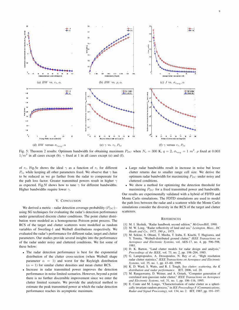
9

(a) BW vs. rt, α. (b) BW vs. ρ, α. (c) J vs. σcavg , α

(d) BW versus σcavg , α (e) γ vs. rt, Ptx (f) γ versus rt, Ptx

Fig. 5: Theorem 2 results: Optimum bandwidth for obtaining maximum PDC when Ns = 300 K, q = 2, σtavg = 1 m2. ρ fixed at 0.0031/m2 in all cases except (b). γ fixed at 1 in all cases except (e) and (f).

of rt. Fig.5e shows the ideal γ as a function of rt for differentPtx while keeping all other parameters fixed. We observe that γ hasto be reduced as we go farther from the radar to compensate forthe path loss factor. Greater transmitted powers result in higher γas expected. Fig.5f shows how to tune γ for different bandwidths.Higher bandwidths require lower γ.

V. CONCLUSION

We derived a metric - radar detection coverage probability (PDC ) -using SG techniques for evaluating the radar’s detection performanceunder generalized discrete clutter conditions. The point clutter distri-bution were modeled as a homogeneous Poisson point process. TheRCS of the target and clutter scatterers were modelled as randomvariables of Swerling-1 and Weibull distributions respectively. Weevaluated the radar’s performance for different radar, target and clutterparameters. Our studies provide several insights into the performanceof the radar under noisy and cluttered conditions. We list some ofthese below:

• The radar detection performance is best for the exponentialdistribution of the clutter cross-section (when Weibull shapeparameter α = 1) and worst for the Rayleigh distribution(α = 1) for similar clutter densities and mean clutter RCS.

• Increase in radar transmitted power improves the detectionperformance in noise limited scenarios. However, beyond a pointthere is no further discernible improvement since we enter theclutter limited scenario. We provide the analytical method toestimate the peak transmitted power at which the radar detectionperformance reaches its asymptotic maximum.

• Large radar bandwidths result in increase in noise but lesserclutter returns due to smaller range cell size. We derive theoptimum radar bandwidth for maximizing PDC under noisy andcluttered conditions.

• We show a method for optimizing the detection threshold formaximizing PDC for a fixed transmitted power and bandwidth.

Our results are experimentally validated with a hybrid of FDTD andMonte Carlo simulations. The FDTD simulations are used to modelthe path loss between the radar and a scatterer while the Monte Carlosimulations consider the diversity in the RCS of the target and clutterscatterers.

REFERENCES

[1] M. I. Skolnik, “Radar handbook second edition,” McGrawHill, 1990.[2] M. W. Long, “Radar reflectivity of land and sea,” Lexington, Mass., DC

Heath and Co., 1975. 390 p., 1975.[3] M. Sekine, S. Ohtani, T. Musha, T. Irabu, E. Kiuchi, T. Hagisawa, and

Y. Tomita, “Weibull-distributed ground clutter,” IEEE Transactions onAerospace and Electronic Systems, vol. AES-17, no. 4, pp. 596–598,1981.

[4] D. K. Barton, “Land clutter models for radar design and analysis,”Proceedings of the IEEE, vol. 73, no. 2, pp. 198–204, 1985.

[5] G. Lampropoulos, A. Drosopoulos, N. Rey et al., “High resolutionradar clutter statistics,” IEEE Transactions on Aerospace and ElectronicSystems, vol. 35, no. 1, pp. 43–60, 1999.

[6] K. D. Ward, S. Watts, and R. J. Tough, Sea clutter: scattering, the Kdistribution and radar performance. IET, 2006, vol. 20.

[7] M. Rangaswamy, D. Weiner, and A. Ozturk, “Computer generation ofcorrelated non-gaussian radar clutter,” IEEE Transactions on Aerospaceand Electronic Systems, vol. 31, no. 1, pp. 106–116, 1995.

[8] E. Conte and M. Longo, “Characterisation of radar clutter as a spheri-cally invariant random process,” in IEE Proceedings F (Communications,Radar and Signal Processing), vol. 134, no. 2. IET, 1987, pp. 191–197.

10

[9] S. N. Chiu, D. Stoyan, W. S. Kendall, and J. Mecke, Stochastic geometryand its applications. John Wiley & Sons, 2013.

[10] J. G. Andrews, F. Baccelli, and R. K. Ganti, “A tractable approachto coverage and rate in cellular networks,” IEEE Transactions onCommunications, vol. 59, no. 11, pp. 3122–3134, 2011.

[11] T. Bai and R. W. Heath, “Coverage and rate analysis for millimeter-wavecellular networks,” IEEE Transactions on Wireless Communications,vol. 14, no. 2, pp. 1100–1114, 2014.

[12] A. Thornburg, T. Bai, and R. W. Heath, “Performance analysis of outdoormmwave ad hoc networks,” IEEE Transactions on Signal Processing,vol. 64, no. 15, pp. 4065–4079, 2016.

[13] G. Ghatak, A. De Domenico, and M. Coupechoux, “Coverage analysisand load balancing in hetnets with millimeter wave multi-rat small cells,”IEEE Transactions on Wireless Communications, vol. 17, no. 5, pp.3154–3169, 2018.

[14] A. Zia, J. P. Reilly, J. Manton, and S. Shirani, “An information geometricapproach to ml estimation with incomplete data: application to semiblindmimo channel identification,” IEEE Transactions on Signal Processing,vol. 55, no. 8, pp. 3975–3986, 2007.

[15] Y. Cui, V. K. Lau, and Y. Wu, “Delay-aware bs discontinuous trans-mission control and user scheduling for energy harvesting downlinkcoordinated mimo systems,” IEEE Transactions on Signal Processing,vol. 60, no. 7, pp. 3786–3795, 2012.

[16] S. Beygi, U. Mitra, and E. G. Strom, “Nested sparse approximation:Structured estimation of v2v channels using geometry-based stochasticchannel model,” IEEE Transactions on Signal Processing, vol. 63,no. 18, pp. 4940–4955, 2015.

[17] A. Al-Hourani, R. J. Evans, S. Kandeepan, B. Moran, and H. Eltom,“Stochastic geometry methods for modeling automotive radar interfer-ence,” IEEE Transactions on Intelligent Transportation Systems, vol. 19,no. 2, pp. 333–344, 2017.

[18] A. Munari, L. Simic, and M. Petrova, “Stochastic geometry interferenceanalysis of radar network performance,” IEEE Communications Letters,vol. 22, no. 11, pp. 2362–2365, 2018.

[19] P. Ren, A. Munari, and M. Petrova, “Performance tradeoffs of jointradar-communication networks,” IEEE Wireless Communications Let-ters, vol. 8, no. 1, pp. 165–168, 2018.

[20] J. Park and R. W. Heath, “Analysis of blockage sensing by radars inrandom cellular networks,” IEEE Signal Processing Letters, vol. 25,no. 11, pp. 1620–1624, 2018.

[21] Z. Fang, Z. Wei, X. Chen, H. Wu, and Z. Feng, “Stochastic geometryfor automotive radar interference with rcs characteristics,” IEEE WirelessCommunications Letters, 2020.

[22] X. Chen, R. Tharmarasa, M. Pelletier, and T. Kirubarajan, “Integratedclutter estimation and target tracking using poisson point processes,”IEEE Transactions on Aerospace and Electronic Systems, vol. 48, no. 2,pp. 1210–1235, 2012.

[23] S. M. Kay, Fundamentals of statistical signal processing. Prentice HallPTR, 1993.

[24] M. Di Renzo, “Computational stochastic geometry–on system-levelmodeling, simulation, performance evaluation, optimization, and ex-perimental validation of 5g wireless communication networks,” in2015 International Conference on Communications, Management andTelecommunications (ComManTel). IEEE, 2015, pp. 1–2.

[25] M. Amin, Radar for indoor monitoring: Detection, classification, andassessment. CRC Press, 2017.

[26] M. E. Davis et al., Foliage penetration radar. SciTech Pub., 2011.[27] T. D. Bufler and R. M. Narayanan, “Radar classification of indoor targets

using support vector machines,” IET Radar, Sonar & Navigation, vol. 10,no. 8, pp. 1468–1476, 2016.

[28] Y.-S. Yoon and M. G. Amin, “Spatial filtering for wall-clutter mitigationin through-the-wall radar imaging,” IEEE Transactions on Geoscienceand Remote Sensing, vol. 47, no. 9, pp. 3192–3208, 2009.

[29] R. Solimene and A. Cuccaro, “Front wall clutter rejection methods intwi,” IEEE Geoscience and remote sensing letters, vol. 11, no. 6, pp.1158–1162, 2013.

[30] S. Vishwakarma and S. S. Ram, “Detection of multiple movers basedon single channel source separation of their micro-dopplers,” IEEETransactions on Aerospace and Electronic Systems, vol. 54, no. 1, pp.159–169, 2017.

[31] ——, “Mitigation of through-wall distortions of frontal radar imagesusing denoising autoencoders,” in IEEE Transactions on Geoscience andRemote Sensing. IEEE, 2020.

[32] S. S. Ram, G. Singh, and G. Ghatak, “Estimating radar detection cover-age probability of targets in a cluttered environment using stochasticgeometry,” in 2020 IEEE International Radar Conference (RADAR).IEEE, 2020, pp. 665–670.

[33] G. Goldstein, “False-alarm regulation in log-normal and weibull clutter,”IEEE Transactions on Aerospace and Electronic Systems, no. 1, pp. 84–92, 1973.

[34] D. Schleher, “Radar detection in weibull clutter,” IEEE Transactions onAerospace and Electronic Systems, no. 6, pp. 736–743, 1976.

[35] E. Conte, A. De Maio, and C. Galdi, “Statistical analysis of real clutterat different range resolutions,” IEEE Transactions on Aerospace andElectronic Systems, vol. 40, no. 3, pp. 903–918, 2004.

[36] M. Haenggi, Stochastic geometry for wireless networks. CambridgeUniversity Press, 2012.

[37] D. Ebdon, “Statistics in geography second edition: A practical approach,”Malden, MA: Blackwell Publishing, 1985.

[38] T. D. Bufler, “Radar signature analysis of indoor clutter and stationaryhuman target classification,” 2016.

[39] S. S. Ram, “Radar simulation of human activities in non line-of-sightenvironments,” Ph.D. dissertation, University of Texas at Austin, 2009.

[40] S. S. Ram, C. Christianson, Y. Kim, and H. Ling, “Simulation andanalysis of human micro-dopplers in through-wall environments,” IEEETransactions on Geoscience and remote sensing, vol. 48, no. 4, pp.2015–2023, 2010.

[41] S. S. Ram and A. Majumdar, “Through-wall propagation effects ondoppler-enhanced frontal radar images of humans,” in 2016 IEEE RadarConference (RadarConf). IEEE, 2016, pp. 1–6.

[42] S. Vishwakarma, A. Rafiq, and S. S. Ram, “Micro-doppler signaturesof dynamic humans from around the corner radar,” in 2020 IEEEInternational Radar Conference (RADAR). IEEE, 2020, pp. 169–174.

[43] G. Ruck, Radar Cross Section Handbook: Volume 1. Springer, 1970,vol. 1.