Embed Size (px)
Citation preview
University of Ottawa
Optimization of Modulation
Constrained Digital Transmission
Systems
by
Yu Han
A thesis submitted in fulfillment for the
degree of Master of Applied Science
in the
Faculty of Engineering
c© Yu Han, Ottawa, Canada, 2017
Abstract
The regular waterfilling(WF) policy maximizes the mutual information of parallel
channels, when the inputs are Gaussian. However, Gaussian input is ideal, which
does not exist in reality. Discrete constellations are usually used instead, such
as M -PAM and M -QAM. As a result, the mercury/waterfilling (MWF) policy
is introduced, which is a generalization of the regular WF. The MWF applies to
inputs with arbitrary distributions, while the regular WF only applies to Gaussian
inputs. The MWF-based optimal power allocation (OPA) is presented, for which
an algorithm called the internal/external bisection method is introduced.
The constellation-constrained capacity is discussed in the thesis, where explicit
expressions are presented. The expression contains an integral, which does not
have a closed-form solution. However, it can be evaluated via the Monte Carlo
method. An approximation of the constellation-constrained capacity based on
the sphere packing method is introduced, whose OPA is a convex optimization
problem. The CVX was used initially, but it did not generate satisfactory results.
Therefore, the bisection method is used instead.
Capacities of the MWF and its sphere packing approximation are evaluated for
various cases, and compared with each other. It turns out the sphere packing
approximation has similar performances to the MWF, which validates the approx-
imation. Unlike the MWF, the sphere packing approximation does not suffer from
the loss of precision due to the structure of MMSE functions, which demonstrates
its robustness.
ii

Acknowledgements
First and foremost, I would like to thank my supervisor, Dr. Sergey Loyka, for
supporting me by providing constructive feedback for my work. It is valuable to me
as it expands my knowledge and gives me a better understanding of communication
systems. I am challenged to be a better academic writer as I realize the importance
of proper writing skills through Dr. Loyka’s supportive comments.
I would like to thank my fellow researcher, Limeng Dong, for being supportive
when I had difficulties. He provides me with new perspectives that allow me to
look at problems at a different angle. His suggestions and comments are much
appreciated.
I owe a special thanks to my friend Cristina Doan, for doing proof reading on my
thesis. Thank you for all the time and efforts you have put in it despite the long
work hours of yours. It gives me understanding about how to write properly, and
makes me a better writer in general.
Last but not the least, I would like to thank my parents for their continuous
support of my study, both financially and mentally. I could not have made it this
far without their support, as it is the foundation of what I have achieved so far.
The past two years of studying have been quite a journey, especially with the
past year working on my thesis. I now realize the difficulty and effort needed to
complete a graduate thesis. It is a precious experience that I will never forget.
iii
Contents
Abstract ii
Acknowledgements iii
Abbreviations vi
List of Symbols viii
1 Introduction 1
1.1 Motivation . . . . . . . . . . . . . . . . . . . . . . . . . . . . . . . . 1
1.2 Digital Transmission System . . . . . . . . . . . . . . . . . . . . . . 2
1.3 The Contributions of the Thesis . . . . . . . . . . . . . . . . . . . . 4
1.4 Thesis Outline . . . . . . . . . . . . . . . . . . . . . . . . . . . . . . 5
2 Literature Review 8
2.1 The Gaussian Channel Capacity . . . . . . . . . . . . . . . . . . . . 8
2.2 Capacity of Memoryless Channels . . . . . . . . . . . . . . . . . . . 9
2.3 The Constellation Capacity . . . . . . . . . . . . . . . . . . . . . . 10
2.4 The Optimal Power Allocation (OPA) . . . . . . . . . . . . . . . . 11
2.5 Convex Optimization . . . . . . . . . . . . . . . . . . . . . . . . . . 14
2.6 The Bisection Method . . . . . . . . . . . . . . . . . . . . . . . . . 14
2.7 Sphere Packing Approximation . . . . . . . . . . . . . . . . . . . . 16
2.8 Summary . . . . . . . . . . . . . . . . . . . . . . . . . . . . . . . . 18
3 The OPA for Finite Constellations: The MWF 20
3.1 System Model of Parallel Channels . . . . . . . . . . . . . . . . . . 20
3.2 Power Normalization . . . . . . . . . . . . . . . . . . . . . . . . . . 21
3.3 Problem Formulation . . . . . . . . . . . . . . . . . . . . . . . . . . 21
3.4 MMSE Functions for Different Constellations . . . . . . . . . . . . . 23
3.5 Low- and High-Power Expansions . . . . . . . . . . . . . . . . . . . 28
3.6 Summary . . . . . . . . . . . . . . . . . . . . . . . . . . . . . . . . 30
iv
Contents v
4 Computation of the OPA 32
4.1 The Mercury/Waterfilling . . . . . . . . . . . . . . . . . . . . . . . 32
4.2 Calculating the Water Level 1/η . . . . . . . . . . . . . . . . . . . . 33
4.3 The Internal/External Bisection Method . . . . . . . . . . . . . . . 34
4.4 Graphic Interpretation of Theorem 3.2 . . . . . . . . . . . . . . . . 37
4.5 A High-Power Approximation . . . . . . . . . . . . . . . . . . . . . 40
4.6 Summary . . . . . . . . . . . . . . . . . . . . . . . . . . . . . . . . 44
5 Approximations of the Constellation Capacity 46
5.1 The Constellation-Constrained Capacity . . . . . . . . . . . . . . . 46
5.2 The Monte Carlo Method . . . . . . . . . . . . . . . . . . . . . . . 48
5.3 The Sphere Packing Approximation . . . . . . . . . . . . . . . . . . 49
5.4 The Constellation-Constrained Waterfilling . . . . . . . . . . . . . . 53
5.5 Another Analytical Approximation . . . . . . . . . . . . . . . . . . 60
5.6 Summary . . . . . . . . . . . . . . . . . . . . . . . . . . . . . . . . 65
6 Performance Analysis of the MWF and its Approximations 66
6.1 Two Parallel Channels . . . . . . . . . . . . . . . . . . . . . . . . . 66
6.2 Three Parallel Channels . . . . . . . . . . . . . . . . . . . . . . . . 90
6.3 Summary . . . . . . . . . . . . . . . . . . . . . . . . . . . . . . . . 99
7 Conclusion 100
7.1 Thesis Summary . . . . . . . . . . . . . . . . . . . . . . . . . . . . 100
7.2 Future research . . . . . . . . . . . . . . . . . . . . . . . . . . . . . 101
Appendix A 103
A.1 History from 1G to 5G . . . . . . . . . . . . . . . . . . . . . . . . . 103
A.2 Proof of Theorem 3.2 . . . . . . . . . . . . . . . . . . . . . . . . . . 106
A.3 Derivation of (3.33) . . . . . . . . . . . . . . . . . . . . . . . . . . . 108
A.4 Derivation of (4.11) . . . . . . . . . . . . . . . . . . . . . . . . . . . 110
A.5 Proof of Theorem 5.1 . . . . . . . . . . . . . . . . . . . . . . . . . . 110
A.6 Proof of Theorem 5.2 . . . . . . . . . . . . . . . . . . . . . . . . . . 111
A.7 Derivation of The Regular Waterfilling from Theorem 5.2 . . . . . . 113
References 114
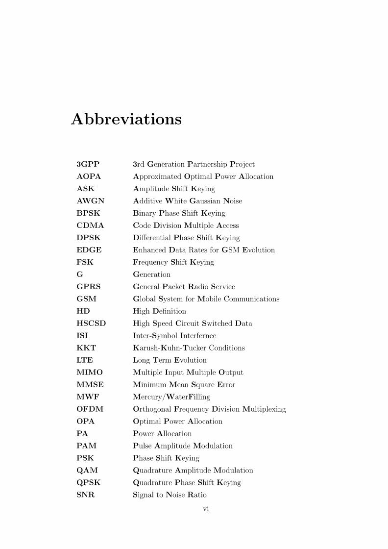
Abbreviations
3GPP 3rd Generation Partnership Project
AOPA Approximated Optimal Power Allocation
ASK Amplitude Shift Keying
AWGN Additive White Gaussian Noise
BPSK Binary Phase Shift Keying
CDMA Code Division Multiple Access
DPSK Differential Phase Shift Keying
EDGE Enhanced Data Rates for GSM Evolution
FSK Frequency Shift Keying
G Generation
GPRS General Packet Radio Service
GSM Global System for Mobile Communications
HD High Definition
HSCSD High Speed Circuit Switched Data
ISI Inter-Symbol Interfernce
KKT Karush-Kuhn-Tucker Conditions
LTE Long Term Evolution
MIMO Multiple Input Multiple Output
MMSE Minimum Mean Square Error
MWF Mercury/WaterFilling
OFDM Orthogonal Frequency Division Multiplexing
OPA Optimal Power Allocation
PA Power Allocation
PAM Pulse Amplitude Modulation
PSK Phase Shift Keying
QAM Quadrature Amplitude Modulation
QPSK Quadrature Phase Shift Keying
SNR Signal to Noise Ratio
vi
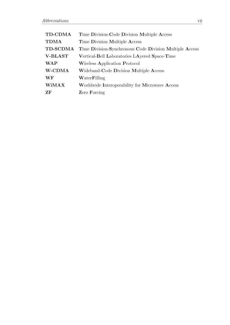
Abbreviations vii
TD-CDMA Time Division-Code Division Multiple Access
TDMA Time Division Multiple Access
TD-SCDMA Time Division-Synchronous Code Division Multiple Access
V-BLAST Vertical-Bell Laboratories LAyered Space-Time
WAP Wireless Application Protocol
W-CDMA Wideband-Code Division Multiple Access
WF WaterFilling
WiMAX Worldwide Interoperability for Microwave Access
ZF Zero Forcing
List of Symbols
B Bandwidth
C Channel capacity
C2 An analytical approximation for the constellation capacity of 2-PAM
C4 An analytical approximation for the constellation capacity of 4-QAM
Cc Sphere packing approximation of the constellation capacity
cL Constellation points
CM Constellation-constrained capacity
d The minimum distance between two constellation points
dij Distance between two constellation points
ε Precision
η Lagrangian multiplier
gk Power gain on the kth channel
γi SNR on the ith channel when power allocation is uniform
h Channel gain
hi Channel gain on the ith channel
I Mutual information
l Lower bound for the bisection method
λ Lagrangian multiplier
m Middle point for the bisection method
M Constellation cardinality
Mk Constellation cardinality on the kth channel
n The number of parallel channels
N The number of distinct codewords that can be transmitted over the channel
Nc The number of distinct codewords that can be transmitted over the channel
under constellation constraint
P Average power of the channels
pi Power allocation on the ith channel
viii
List of Symbols ix
p∗i Optimal power allocation on the ith channel
PT Total power
p(x, y) Joint probability density function
p(x), p(y) Marginal probability density functions
qL Probability of taking a constellation point
ρ SNR
si Normalized unit-power input
σ2 Noise power of the channel
u Upper bound for the bisection method
VM Codeword region volume
w Channel noise
wi Noise of the ith channel
x Input of the channel
xi Input of the ith channel
y Output of the channel
yi Output of the ith channel
Chapter 1
Introduction
1.1 Motivation
Over the past few years, the usage of wireless devices have increased worldwide.
The increase in usage of these devices have created a demand for more download-
able applications. A large number of applications now require Internet connection
in order to function. In such case, the speed of the Internet is crucial for user
experience, and so is the stability. With applications becoming more complex, it
has created a need for an increase in quality, as well as a higher rate of Internet
service. Several generations of technologies have already been developed in order
for mobile communication devices to reach the current standards, ranging from 1G
to 4G. The review of their history and development can be found in the Appendix
A.1.
Battery life is also another important factor that affect the quality of mobile
devices. A trade-off exists between power and rate, which is the reason why the
optimization of data rates within a total power budget is imperative. In reality,
the objective is to acquire higher rates with the lowest possible transmit power.
The existing issue of this trade-off is expected to be resolved by the upcoming 5th
generation (5G) of cellular systems. With the development of new technologies, it
will soon be possible to acheive higher rates with a lower transmit power.
The upcoming 5G includes several key enabling technologies, such as massive
MIMO, millimeter waves, and heterogenous networks. A detailed introduction to
1
Chapter 1. Introduction 2
these technologies, as well as the review of previous standards and protocols can
be found in the Appendix A.1.
Massive MIMO is an upgraded version of MIMO, of which the number of antennas
at the transmitter and the receiver is increased tremendously. A greater number
of antennas in combination with multipath propagation allows for higher rates.
Millimeter wave technology exploits the ultra high frequency bands from 30 GHz
to 300 GHz, due to the fact that it is already congested at lower frequency bands.
As a result, bandwidths, as well as data rates will increase.
As discussed above, power efficiency is also a contributing factor to quality of
mobile devices. Both battery life and data rates are crucial for users, therefore
the optimization of data rates under a given power budget becomes an important
topic considered in this thesis. In addition, the optimization problem of power
allocation subject to the a capacity constraint is also resolved, due to the fact that
the two optimization problems above are equivalent to each other.
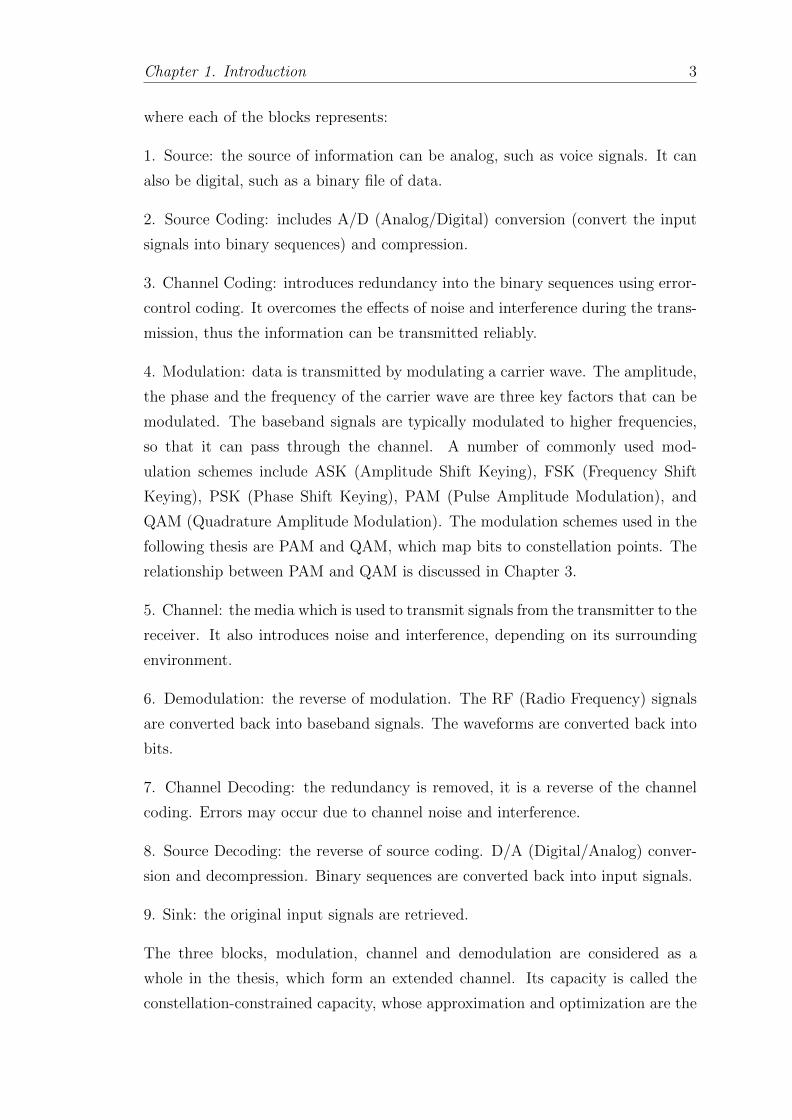
1.2 Digital Transmission System
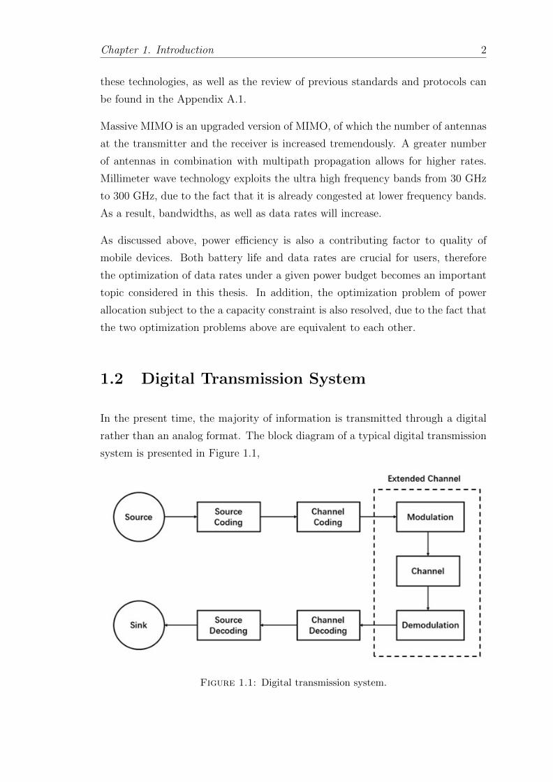
In the present time, the majority of information is transmitted through a digital
rather than an analog format. The block diagram of a typical digital transmission
system is presented in Figure 1.1,
Figure 1.1: Digital transmission system.
Chapter 1. Introduction 3
where each of the blocks represents:
1. Source: the source of information can be analog, such as voice signals. It can
also be digital, such as a binary file of data.
2. Source Coding: includes A/D (Analog/Digital) conversion (convert the input
signals into binary sequences) and compression.
3. Channel Coding: introduces redundancy into the binary sequences using error-
control coding. It overcomes the effects of noise and interference during the trans-
mission, thus the information can be transmitted reliably.
4. Modulation: data is transmitted by modulating a carrier wave. The amplitude,
the phase and the frequency of the carrier wave are three key factors that can be
modulated. The baseband signals are typically modulated to higher frequencies,
so that it can pass through the channel. A number of commonly used mod-
ulation schemes include ASK (Amplitude Shift Keying), FSK (Frequency Shift
Keying), PSK (Phase Shift Keying), PAM (Pulse Amplitude Modulation), and
QAM (Quadrature Amplitude Modulation). The modulation schemes used in the
following thesis are PAM and QAM, which map bits to constellation points. The
relationship between PAM and QAM is discussed in Chapter 3.
5. Channel: the media which is used to transmit signals from the transmitter to the
receiver. It also introduces noise and interference, depending on its surrounding
environment.
6. Demodulation: the reverse of modulation. The RF (Radio Frequency) signals
are converted back into baseband signals. The waveforms are converted back into
bits.
7. Channel Decoding: the redundancy is removed, it is a reverse of the channel
coding. Errors may occur due to channel noise and interference.
8. Source Decoding: the reverse of source coding. D/A (Digital/Analog) conver-
sion and decompression. Binary sequences are converted back into input signals.
9. Sink: the original input signals are retrieved.
The three blocks, modulation, channel and demodulation are considered as a
whole in the thesis, which form an extended channel. Its capacity is called the
constellation-constrained capacity, whose approximation and optimization are the
Chapter 1. Introduction 4
major contributions of the thesis. PAM and QAM are the two types of modulation
scheme considered in the thesis, and details of the other modulation schemes can
be found in Chapter 2. Four constellation schemes, 4-QAM, 16-QAM, 64-QAM
and 256-QAM are applied to specific channels in Chapter 6. While the general
results apply, higher order constellations are not considered in detail due to their
complexity.
Parallel channels (such as OFDM channels with distinct carrier frequencies) are
used as a model within this thesis. An approximation of the modulation con-
strained capacity is introduced. The corresponding power allocation is required to
maximize the constellation capacity subject to the power constraint. A convex op-
timization problem arises, which can be solved using KKT (Karush-Kuhn-Tucker)
conditions.
Convex optimization is a useful tool that can be applied to many optimization
problems. It is highly integrated with programming software such as Matlab. A
package called CVX can be used to solve convex optimization problems. However,
the CVX has a rigorous standard for the recognition of convex functions. The
convex functions have to be presented in a modified form in order for recognition
in most cases, therefore the bisection method is used instead to avoid such issues.
The bisection method is a root-finding algorithm for monotonic functions, whose
specifics are discussed in Chapter 2 with an intuitive flow chart. The optimal
power allocation (OPA) of the constellation capacity can be derived using the
bisection method, which provides better results as compared with the CVX.
1.3 The Contributions of the Thesis
The main references of this thesis are [1] and [2], where several new algorithms are
implemented. The majority of the simulation results in both papers are validated
in the present thesis, most of which agree well with our results. However, in the
process of validation, a few errors in [1] are found and corrected.
Reference [1] provides the MMSE-based mercury/waterfilling (MWF) solution for
parallel channels with arbitrary input distributions, while [2] utilizes the sphere
packing method to obtain an approximation of the constellation capacity. It is
then used to obtain the OPA for parallel channels.
Chapter 1. Introduction 5
One of the main contributions to this thesis is the utilization of the bisection
method to obtain the OPA. An algorithm based on the bisection method is de-
veloped and implemented, and its performance is compared with the CVX. As
a result, the bisection method is shown to be more robust than the CVX. The
utilization of the CVX resulted in abnormal behaviours, which are discussed in
Chapter 5.
Another major contribution is the comparison between different power alloca-
tion schemes, including MWF, constellation-constrained waterfilling based on the
sphere packing approximation, and regular waterfilling (WF). Their performances
are studied via their respective capacities. At a selected SNR, the higher the ca-
pacity is, the better the performance. The case of two parallel channels is studied
in detail with different constellation cardinalities and channel gains. Afterwards,
a case of three parallel channels is considered in comparison with the case of two
parallel channels.
The performance difference between the MWF and the constellation-constrained
WF (AOPA) is found to be insignificant. The sphere packing approximation is
considerably easier to evaluate, it requires less time and demonstrates robust per-
formance. More importantly, unlike the MMSE-based MWF, it does not drop to
zero abnormally in the high SNR region due to the loss of precision. Therefore, it
is considered to be a valuable tool for system design and optimization.
In the thesis, the same constellation is applied to all the sub-channels for the
optimization problem. As an extension, adaptive modulation can be considered,
applying different modulation schemes to different sub-channels depending on their
respective channel gains. The optimization of PA with adaptive modulation will
be an interesting topic for future research.
1.4 Thesis Outline
The remainder of the thesis is organized as follows:
Chapter 2 gives the literature review. The capacity is introduced, such as the
Gaussian channel capacity and the constellation-constrained capacity. An ap-
proximation of the constellation capacity based on sphere packing is presented.
Chapter 1. Introduction 6
Corresponding power allocation policies are given, and convex optimization is
used in the process of obtaining the OPA.
Chapter 3 presents the system model of parallel channels. The general power
constraint is discussed in this chapter, along with the power normalization in
[1]. A new normalized power constraint is introduced, and then the SNR of the
uniform power allocation (PA) is defined. The rest of this chapter deals with
the OPA under modulation constraint. The MWF is introduced in [1] as the
OPA scheme for parallel channels with arbitrary input distributions. There is no
explicit closed form expression, due to the presence of MMSE (Minimum Mean
Square Error) functions that contain integrals. A general expression for the MMSE
functions is introduced, as well as expressions for specific constellations. A number
of basic characteristics of constellations and their corresponding MMSE functions
are discussed. Finally, a low and a high-power expansion of the MMSE functions
are introduced, which will be useful in the upcoming chapters.
Chapter 4 focuses on the evaluation of the OPA. The MMSE function appears in
the expressions. As a result, the OPA cannot be derived directly. The bisection
method is used for the derivation of the OPA. For the bisection method to start,
upper and lower bounds are derived at first, and then the OPA can be calculated
with a given precision. A graphic interpretation of the OPA is given in this chapter.
A high-power approximation is introduced based on the high-power expansion in
Chapter 3. The capacity of the MWF and its high-power approximation are
compared. The high-power approximation fits the exact MWF well in the high
SNR region.
Chapter 5 provides the detailed discussion of the modulation constrained capacity.
Gaussian channel capacity is initially addressed, and then the constellation capac-
ity. The Monte Carlo method is used to evaluate the constellation capacity due
to its complexity. It converts the integral inside the expression into the mean of a
Gaussian random variable. This is essential when performing the numerical eval-
uation using Matlab. Moreover, an approximation of the constellation capacity
based on sphere packing is presented, along with its approximated OPA (AOPA).
A different approach of approximation is proposed at the end of this chapter. It
provides a greater accuracy, but it only applies to 2-PAM after certain manipu-
lations. It is also difficult to extend to higher order constellations, therefore this
direction is no longer persued.
Chapter 1. Introduction 7
Chapter 6 compares the performance of the MWF and the sphere packing ap-
proximation. Other power allocation schemes are used as well for comparison,
such as regular WF, the uniform PA, and the OPA derived with the Monte Carlo
method. As special cases, two parallel channels are initially investigated, with dif-
ferent constellation cardinalities and channel gains. Subsequently, three parallel
channels with the same constellation cardinalities and channel gains are considered
for comparison. As shown in all the figures in this chapter, the sphere packing
approximation is a close fit for the MMSE-based MWF OPA. It is also simplier
and more efficient to evaluate. Their curves all saturate eventually as the SNR
increases due to the upper bound on the constellation capacity, which is deter-
mined by the constellation cardinality. Capacity cannot exceed the upper bound
no matter how high the SNR is.
Chapter 2
Literature Review
2.1 The Gaussian Channel Capacity
For a channel with only one transmitter and one receiver, channel capacity stands
for the maximum quantity of information transmitted every second or every symbol
which is measured in bits/s or bits/symbol. In other words, it is the upper bound of
data rate at which information can be transmitted reliably. Reliable transmission
here means that information can be transmitted at an arbitrarily low error rate.
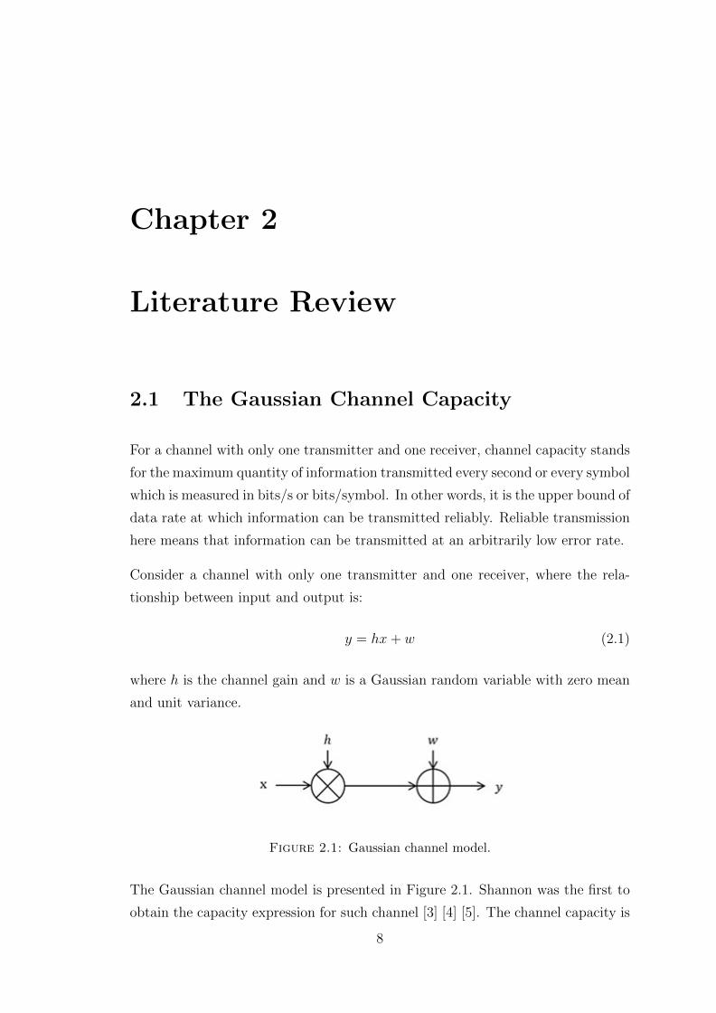
Consider a channel with only one transmitter and one receiver, where the rela-
tionship between input and output is:
y = hx+ w (2.1)
where h is the channel gain and w is a Gaussian random variable with zero mean
and unit variance.
Figure 2.1: Gaussian channel model.
The Gaussian channel model is presented in Figure 2.1. Shannon was the first to
obtain the capacity expression for such channel [3] [4] [5]. The channel capacity is
8
Chapter 2. Literature Review 9
proportional to bandwidth and related to SNR, as presented below:
C = B log2(1 + SNR) [bits/s] (2.2)
where B is bandwidth of the channel which is measured in Hz, and SNR is the
signal to noise ratio of the channel.
Shannon pointed out that if data rate R is less than channel capacity C, then
theoretically there is a way to transmit the information through the channel at an
arbitrarily low error probability. However, if R is greater than C, then under no
circumstances can the information be transmitted reliably [4].
2.2 Capacity of Memoryless Channels
A memoryless channel is a channel for which the output at time t is determined
only by the input at time t and not influenced by any input prior to or after time
t. On the contrary, a channel with memory is a channel for which the output at
time t is affected by some inputs prior to or after time t.
For stationary memoryless channels, the channel capacity can be expressed as the
maximum mutual information:
C = maxX
I(X;Y ) [bits/symbol] (2.3)
where X is the random variable which is transmitted and Y is the random variable
which is received; I(X;Y ) is the mutual information between X and Y . Assuming
X and Y are discrete random variables, the mutual information I(X;Y ) can be
further expanded as:
I(X;Y ) =∑x,y
p(x, y) logp(x, y)
p(x)p(y)(2.4)
where p(x, y) is the joint probability distribution, p(x) and p(y) are the marginal
probability distributions.
For continuous random variables, the only difference in mutual information ex-
pression is the replacement of the summation in (2.4) with an integral. Moreover,
capacity for channels with memory is discussed in [6].
Chapter 2. Literature Review 10
2.3 The Constellation Capacity
The Shannon formula (2.2) only applies to Gaussian channels, for which there
are no constraints on modulation or coding. Some of the criteria for choosing
the right modulation scheme include power efficiency, bandwidth efficiency, and
system complexity [7]. There are several different types of modulations [7] [8],
such as PAM (Pulse Amplitude Modulation), PSK (Phase Shift keying), FSK
(Frequency Shift keying), ASK (Amplitude Shift keying) and QAM (Quadrature
Amplitude Modulation) [9]. PAM encodes the information in the amplitude of
the waveform. PSK modifies the phase of the carrier wave, and the information is
embedded in the phase. It has a variation, DPSK, which is similar to PSK, but the
information is encoded in the difference between successive phases. As for FSK,
the information is transmitted through the frequency changes of the carrier wave.
ASK is another scheme whose information lies in the amplitude of the carrier wave.
M -QAM can be seen as a combination of two√M -PAM in quadrature. There are
two carrier waves with the same frequency but they have a 90 degrees of phase
difference [10]. PAM and QAM are the two schemes that considered in this thesis,
their relationship discussed above is important for MMSE functions which will be
discussed later.
The constellation cardinality M (i.e. the number of constellation points) has
an influence on the capacity as well as the modulation schemes. The higher M
is, the closer it is to Gaussian channel capacity [11]. Unlike all the modulation
schemes above which are uniformly-spaced, [12] considers non-uniformly spaced
constellations and corresponding capacity is evaluated for comparison.
The expression of the constellation capacity for M -PAM can be found in [13] and
[14]. Some of its properties can be found in [15]. An example of two-user broadcast
channels can be found in [16]. The explicit expression is as follows:
CM = log2M −∑j
1
M
∫ ∞−∞
1√2πσ2
e−z2
2σ2 log2
∑i
e−d2ij2σ2 e−
zdij
σ2 dz (2.5)
where M is the constellation order, σ2 = N is the noise power of the channel, and
z is a Gaussian random variable with zero mean and a variance of σ2. The average
power is normalized to be 1, so that SNR = 1σ2 .
Chapter 2. Literature Review 11
In the thesis, the expression above is used to calculate the capacity of the mer-
cury/weaterfilling and some other power allocation schemes to evaluate their per-
formances. However, the expression is quite complex due to the integral and it
does not have a closed form solution [17] [18]. The Monte Carlo method is used
instead in order to calculate the integral.
The Monte Carlo method was developed in mid 1940s. It is an algorithm that ex-
ploits randomness to obtain numerical results [19] [20]. In our case, the integral in
the constellation capacity expression can be dealt with properly using the Monte
Carlo method. Clearly 1√2πσ2
e−z2
2σ2 is a Gaussian probability density function. The
integral can be treated as the calculation of the mean of a Gaussian random vari-
able z with zero mean and a variance of σ2. More details about the constellation
capacity and the Monte Carlo method can be found in Chapter 6.
2.4 The Optimal Power Allocation (OPA)
Now that the capacity expression is presented in (2.5), it is natural to seek for an
OPA scheme that maximizes channel capacity under a fixed total power budget.
The OPA for parallel channels is an optimization problem which usually emerges in
the transmitter design. For such parallel channels, which are mutually independent
and with Gaussian inputs, the well-known waterfilling (WF) policy is the OPA
scheme that maximizes the mutual information [3] [21].
Algorithms for evaluating the WF can be found in [22], that are applied to compute
the numerical solutions in practice. A family of different WF solutions is discussed
[22] as well, along with their comparisons. Specifically, constant-power WF is
stated in [23]. It can be used on wireless fading channels and wireline channels
with ISI (Inter-Symbol Interference).
The WF algorithm is the classic power allocation scheme for Gaussian channels
[24] as it is an elegant solution with intuitive graphic interpretation. It utilizes the
concavity of the capacity expression, and convex optimizaion is used to obtain the
OPA.
Chapter 2. Literature Review 12
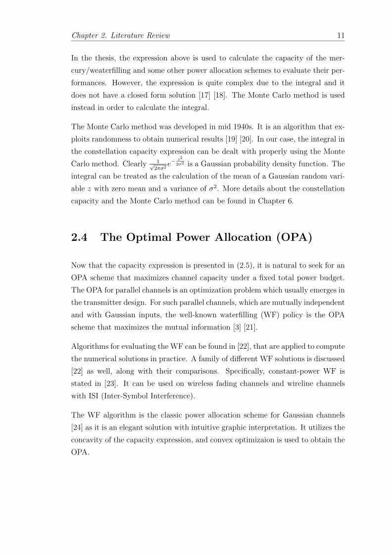
Consider n parallel channels fed with Gaussian inputs. Expression for the WF
OPA is as follows:
pi = 0, γi ≤ η (2.6)
pi =1
η− 1
γi, γi > η (2.7)
where 1η
is the water level found from the power constraint, which is discussed
thoroughly in Chapter 4. The term γi is the SNR on the ith channel when the
power allocation is uniform [1].
It is seen clearly from the expressions above that channels with higher SNR receive
more power. There is no power assigned to the channels whose SNR is not higher
than η.
Figure 2.2: Graphic interpretation of the WF policy [1].
Figure 2.2 is the graphic interpretation of the WF policy, 1η
serves as the water
level and 1γi
serves as noise. For n parallel channels, each channel corresponds to a
unit based vessel. The solid part at the bottom of the vessel is set up at a height of1γi
, then water is poured into the vessels until water level in all the vessels reaches1η. The amount of water in each vessel corresponds to the power that is allocated
to that channel.
However, the WF policy only applies when the input is Gaussian [25]. Discrete
constellations are usually used in reality instead of the ideal Gaussian inputs, for
which there is a modified version of the WF policy for arbitrary input distributions,
which is known as the mercury/waterfilling (MWF) [24] [25]. It is similar to the
regular WF, except that a mercury part is added. Some of its applications can be
found in [25], [26] and [27]. A practical use of the MWF over parallel Gaussian
channels in the multiuser context can be found in [28].
Chapter 2. Literature Review 13
The MWF is extensively discussed in [1], [29] and [30]. Its OPA {p∗i } can be
written as [1]:
p∗i = 0, γi 6 η (2.8)
γiMMSEi(p∗i γi) = η, γi > η (2.9)
where MMSE(·) is the minimum mean square error [31].
The MMSE expression varies for different inputs. The general expression is stated
in [1], along with more detailed expressions for specific constellations. A rela-
tionship between MMSE and mutual information is discussed in [1], [32] and [33].
Moreover, the derivatives of MMSE and their properties are discussed in [33] and
[34].
Using (2.8) and (2.9), a new function Gi(ξ) can be constructed for the graphic
interpretation of the MWF [1]:
Gi(ξ) = 1/ξ −MMSE−1i (ξ), 0 ≤ ξ ≤ 1 (2.10)
Gi(ξ) = 1, ξ > 1 (2.11)
where MMSE−1i (·) is the inverse of MMSE functions.
For Gaussian inputs, Gi(ξ) = 1 holds for all ξ. For other inputs with discrete
constellations, the inverse of the specific MMSE function is required in order to
acquire Gi(ξ). Some of the MMSE functions for specific constellation are presented
in [1] and the others can be derived from the general expression. Using Gi(ξ), the
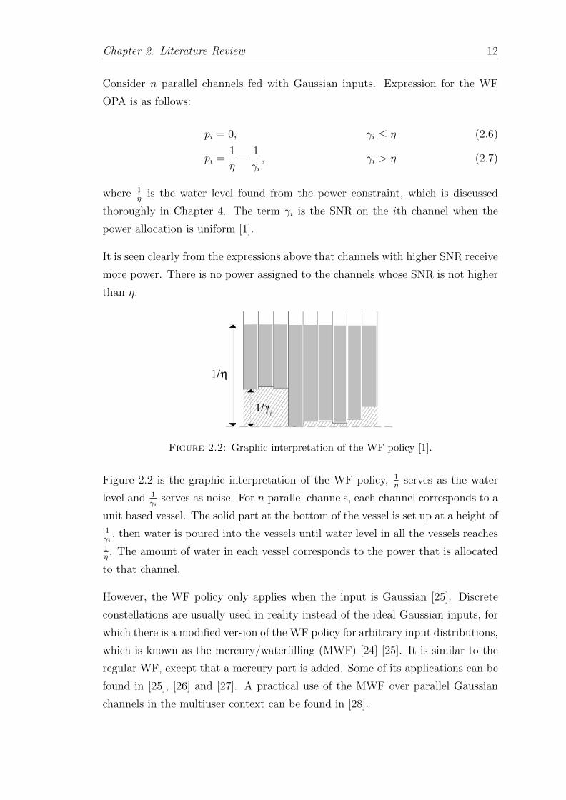
MWF can be illustrated better with just a few steps shown below:
1. It is similar to the regular WF. For all the channels, set up a unit based vessel
solid up to a height of 1/γi.
2. Determine η, pour ”mercury” into all the vessels until the level of mercury
(including the solid part) reaches Gi(η/γi)/γi.
3. Pour ”water” into all the vessels until the level of water reaches 1/η.
4. The height of water over the mercury is the OPA p∗i for the ith channel.
The graphic interpretation is in Figure 2.3. Pouring mercury onto a vessel amounts
to raising the noise level in that channel by an amount that depends on the input
Chapter 2. Literature Review 14
Figure 2.3: Graphic interpretation of the MWF [1].
distribution [1]. It can also be interpreted as the gap to ideal Gaussian input.
More details on the MWF are discussed in Chapter 5.
2.5 Convex Optimization
Convex optimization is a useful tool for min/max problems. It requires the ob-
jective and constraints to be convex [35]. More importantly, it is integrated into
softwares, such as Matlab, and a package called CVX is available [36]. It can be
used to solve convex optimization problems directly, but the convex problem and
constraints need to be properly formed first. However, it cannot recognize convex
functions properly every time, therefore they have to be presented in a modified
form so that they can be recognized as convex.
At first, we used the CVX for simulations, but the results were not satisfying and
there were gaps on the curves which were abnormal. After some efforts, it was
decided to not use the CVX anymore. The bisection method is used instead to
solve the power allocation optimization problems.
2.6 The Bisection Method
The bisection method is an approach of finding the root of a function1. The
method itself is quite simple but powerful. When considering a monotonically
decreasing function f(x), the bisection method can be applied to obtain the root
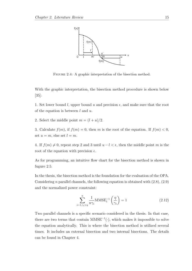
of the equation f(x) = 0. A graphic interpretaion is shown in Figure 2.4,
1Not necessarily a monotonic function. In our case, the function is monotonic.
Chapter 2. Literature Review 15
Figure 2.4: A graphic interpretation of the bisection method.
With the graphic interpretation, the bisection method procedure is shown below
[35]:
1. Set lower bound l, upper bound u and precision ε, and make sure that the root
of the equation is between l and u.
2. Select the middle point m = (l + u)/2.
3. Calculate f(m), if f(m) = 0, then m is the root of the equation. If f(m) < 0,
set u = m, else set l = m.
4. If f(m) 6= 0, repeat step 2 and 3 until u− l < ε, then the middle point m is the
root of the equation with precision ε.
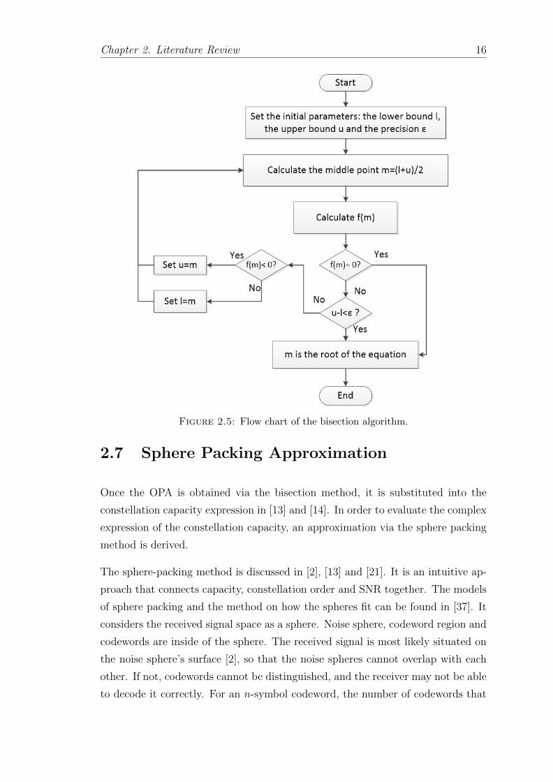
As for programming, an intuitive flow chart for the bisection method is shown in
fugure 2.5.
In the thesis, the bisection method is the foundation for the evaluation of the OPA.
Considering n parallel channels, the following equation is obtained with (2.8), (2.9)
and the normalized power constraint:
n∑i=1,γi>η
1
nγiMMSE−1i
(η
γi
)= 1 (2.12)
Two parallel channels is a specific scenario considered in the thesis. In that case,
there are two terms that contain MMSE−1(·), which makes it impossible to solve
the equation analytically. This is where the bisection method is utilized several
times. It includes an external bisection and two internal bisections. The details
can be found in Chapter 4.
Chapter 2. Literature Review 16
Figure 2.5: Flow chart of the bisection algorithm.
2.7 Sphere Packing Approximation
Once the OPA is obtained via the bisection method, it is substituted into the
constellation capacity expression in [13] and [14]. In order to evaluate the complex
expression of the constellation capacity, an approximation via the sphere packing
method is derived.
The sphere-packing method is discussed in [2], [13] and [21]. It is an intuitive ap-
proach that connects capacity, constellation order and SNR together. The models
of sphere packing and the method on how the spheres fit can be found in [37]. It
considers the received signal space as a sphere. Noise sphere, codeword region and
codewords are inside of the sphere. The received signal is most likely situated on
the noise sphere’s surface [2], so that the noise spheres cannot overlap with each
other. If not, codewords cannot be distinguished, and the receiver may not be able
to decode it correctly. For an n-symbol codeword, the number of codewords that
Chapter 2. Literature Review 17
can be transmitted reliably is just the number of non-overlapped noise spheres
inside the received signal sphere [2]:
N =α(√nP + nσ2)n
α(√nσ2)n
= (1 + ρ)n/2 (2.13)
where P is the maximum power of each symbol, σ2 is the average noise power per
symbol and ρ is the SNR. α =πn/2
Γ(n2
+ 1), and Γ(·) is the Gamma function.
Therefore in this case channel capacity can be expressed as:
C =1
nlogN =
1
2log(1 + ρ) [bits/s/Hz] (2.14)
After taking M -PAM constellation into cosideration, the number of codewords
becomes Mn. Assuming channel noise is small, the codeword region volume can
be expressed as:
VM =α(√nP )n
Mn= α
(√nP
M
)n
(2.15)
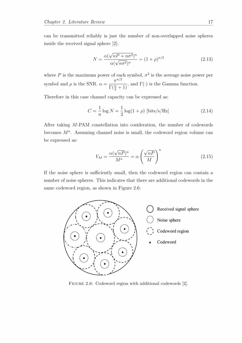
If the noise sphere is sufficiently small, then the codeword region can contain a
number of noise spheres. This indicates that there are additional codewords in the
same codeword region, as shown in Figure 2.6:
Figure 2.6: Codeword region with additional codewords [2].
Chapter 2. Literature Review 18
Then the number of noise spheres that can fit into the codeword region is:(nPM2 + nσ2
nσ2
)n/2
=(
1 +ρ
M2
)n/2(2.16)
Therefore the number of codewords for M -PAM constellation becomes:
Nc =N(
1 + ρM2
)n/2 =(1 + ρ)n/2(1 + ρ
M2
)n/2 (2.17)
In this case, the constellation capacity for M -PAM can be approximated as [2]:
Cc ≈1
nlogNc ≈
1
2log
1 + ρ
1 + ρM2
(2.18)
This approximation of the constellation capacity is much easier to evaluate com-
pared with (2.5). The OPA in Chapter 6 is derived based on this approximation
using convex optimization. It also has a decent performance compared with the
original expression, and more of its details can be found in Chapter 6.
2.8 Summary
Channel capacity is discussed in this chapter, more specifically, Gaussian chan-
nel capacity and then the constellation capacity. There is an integral inside the
constellation capacity expression which does not have a closed form solution. The
Monte Carlo integration is used to evaluate it. The sphere packing method is
used to obtain an approximation of the constellation capacity since its original
expression is more complicated to evaluate.
With the sphere packing approximation of the constellation capacity, convex op-
timization can be used to compute the OPA. However, problems arise when using
the CVX to compute the OPA, there are abnormal gaps on the curves which are
discussed in Chapter 5. Therefore, the OPA under a total power constraint is com-
puted using the bisection method, since the OPA function is monotonic. Once the
OPA is obtained, it is substituted into the constellation capacity to compare its
performance with the MWF, which is the OPA for parallel channels with arbitrary
input distributions. The regular WF is also briefly discussed in this chapter.
Chapter 2. Literature Review 19
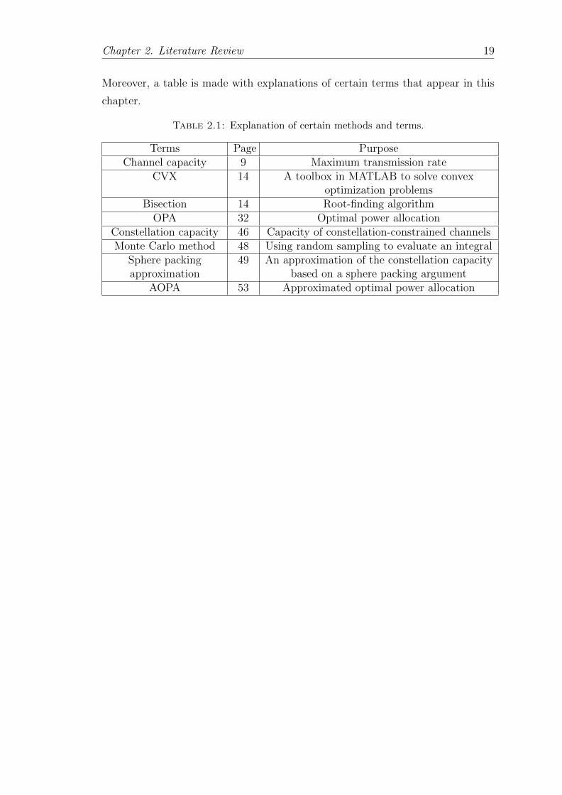
Moreover, a table is made with explanations of certain terms that appear in this
chapter.
Table 2.1: Explanation of certain methods and terms.
Terms Page PurposeChannel capacity 9 Maximum transmission rate
CVX 14 A toolbox in MATLAB to solve convexoptimization problems
Bisection 14 Root-finding algorithmOPA 32 Optimal power allocation
Constellation capacity 46 Capacity of constellation-constrained channelsMonte Carlo method 48 Using random sampling to evaluate an integral
Sphere packingapproximation
49 An approximation of the constellation capacitybased on a sphere packing argument
AOPA 53 Approximated optimal power allocation
Chapter 3
The OPA for Finite
Constellations: The MWF
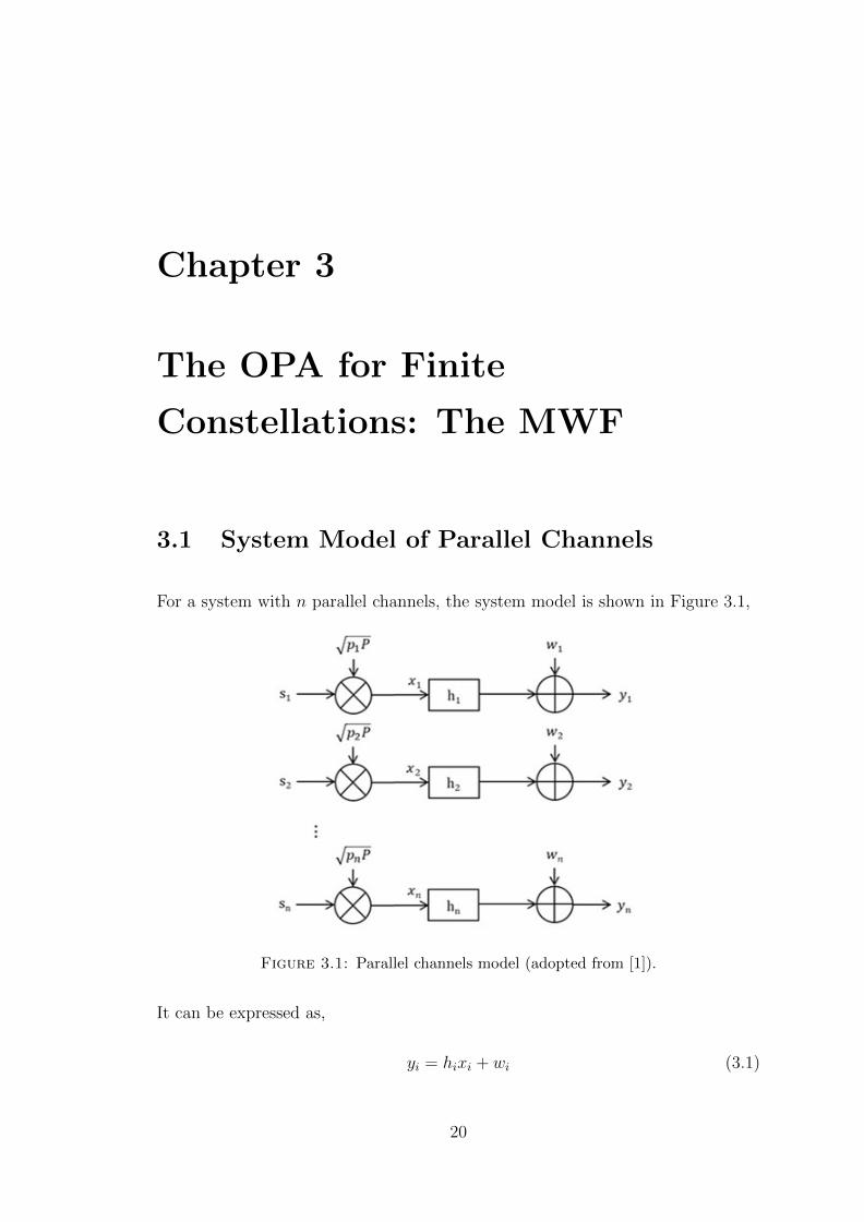
3.1 System Model of Parallel Channels
For a system with n parallel channels, the system model is shown in Figure 3.1,
Figure 3.1: Parallel channels model (adopted from [1]).
It can be expressed as,
yi = hixi + wi (3.1)
20
Chapter 3. The OPA for Finite Constellations: The MWF 21
where wi is i.i.d Gaussian noise, with zero mean and unit variance, hi is the fixed
channel gain which varies for different channels, xi is the channel input and yi is
the channel output.
3.2 Power Normalization
The power constraint can be expressed as
1
n
n∑i=1
E[|xi|2] ≤ P (3.2)
where E(·) is the statistical expectation, and P is the average power constraint.
It is convenient to introduce normalized unit-power inputs si. Its relationship with
the original input xi is
xi =√piPsi (3.3)
where pi is the power allocation of si, so that the new power constraint can be
written as
1
n
n∑i=1
pi ≤ 1 (3.4)
For parallel channels, the following quantity
γi = P |hi|2 (3.5)
is a measure of the strength of the channel, piγi is the SNR of the i-th channel.
Therefore γi is the SNR for uniform power allocation (pi = 1).
3.3 Problem Formulation
In order to increase the spectral efficiency, modulation-constrained mutual infor-
mation is maximized via the OPA. This optimization problem can be expressed
Chapter 3. The OPA for Finite Constellations: The MWF 22
as:
[p∗1, ..., p∗n] = arg max
1
n
n∑i=1
Ii(piγi), s.t.1
n
n∑i=1
pi = 1 (3.6)
where Ii(piγi) is the mutual information and piγi is the SNR mentioned above.
As seen in Theorem 3.2, an important part of this OPA process is the MMSE
functions. The MMSE estimate of si can be expressed as
si(yi, ρ) = E[si|√ρsi + wi = yi] (3.7)
where ρ is the SNR and si is the unit-power input. Therefore the corresponding
mean-square error can be written as
MMSEi(ρ) = E[|si − si(√ρsi + wi, ρ)|2] (3.8)
where MMSEi(ρ) ∈ [0, 1] since si has unit power.
The relationship between mutual information and MMSE functions is introduced
in [1], as shown below:
Theorem 3.1. For any distribution of si (not dependent on ρ)
d
dρIi(ρ) = MMSEi(ρ) (3.9)
The OPA is derived based on the Theorem 3.1 above.
Theorem 3.2. [1] The solution to the OPA problem in (3.6) can be expressed as:
p∗i = 0, γi 6 η (3.10)
γiMMSEi(p∗i γi) = η, γi > η (3.11)
with η > 0 such that
1
n
∑i
p∗i = 1 (3.12)
Proof. See Appendix A.2.
Chapter 3. The OPA for Finite Constellations: The MWF 23
The OPA can be expressed more explicitly as:
p∗i =1
γiMMSE−1i
(min
{1,η
γi
}), i = 1, ..., n (3.13)
where MMSE−1i (·) is the inverse of MMSE functions.
This optimization problem can be solved via KKT conditions, as discussed in the
Appendix A.2. A different approach of the proof can be found in the Appendix of
[1].
The parameter η can be determined by the power normalization (3.12), which can
be further expanded as,
n∑i=1,γi>η
1
nγiMMSE−1i
(η
γi
)= 1 (3.14)
From the two expressions above, it is concluded that η can be solved from (3.14)
and then substituted into (3.13) to obtain the OPA. MMSE expressions for specific
constellations are introduced in the next section.
3.4 MMSE Functions for Different Constellations
For Gaussian inputs, MMSE function can be written as [1],
MMSEi(ρ) =1
1 + ρ(3.15)
so that the inverse of MMSE is
MMSE−1i (ξ) =1
ξ− 1 (3.16)
and Theorem 3.2 reduces to the well-known WF [1],
pi = 0, ri 6 η (3.17)
pi =1
η− 1
γi, γi > η (3.18)
where 1η
is the water level.
Chapter 3. The OPA for Finite Constellations: The MWF 24
For discrete constellations such as M -PAM (Pulse Amplitude Modulation) and M -
QAM (Quadrature Amplitude Modulation), the constellation points are denoted
by cL, where L = 1, 2, ...,M . Each of them is taken with a probabilty of qL (for
most cases, qL = 1/M), which sums up to 1.
For M -PAM,
cL = (2L− 1−M)
√3
M2 − 1(3.19)
For M -QAM, it is made up of two√M -PAM constellations in quadrature, each
with half the power.
With Gaussian noise, the MMSE estimate of input si is [1],
s(y, ρ) =
∑ML=1 qLcLe
−|y−√ρcL|2∑ML=1 qLe
−|y−√ρcL|2(3.20)
The general form of MMSE expression is
MMSE(ρ) =
∫ M∑L=1
qL|cL − s(y, ρ)|2 e−|y−√ρcL|2
√π
dy (3.21)
= 1− 1√π
∫ |∑ML=1 qLcLe
−|y−√ρcL|2|2∑ML=1 qLe
−|y−√ρcL|2dy (3.22)
For (3.21) and (3.22), there is an error discovered in [1]. The denominator is
supposed to be√π instead of π, and it was found when the equation (3.22) was
expanded and compared with the expressions of specific constellations.
For BPSK, which is equivalent to 2-PAM, (3.22) can be expanded as
MMSE(ρ) = 1−∫ +∞
−∞tanh(2
√ρξ)
e−(ξ−√ρ)2
√π
dξ (3.23)
QPSK (or equivalently 4-QAM) consists of two BPSK in quadrature, each with
half the power of BPSK. As a result, the MMSE expression of QPSK or 4-QAM
can be calculated from that of BPSK as follows:
MMSEQPSK(ρ) = MMSEBPSK(ρ
2
)(3.24)
Chapter 3. The OPA for Finite Constellations: The MWF 25
For 4-PAM, (3.22) can be expanded as
MMSE(ρ) = 1−∫ +∞
−∞
(3e−8ρ/5 sinh(6√
ρ5ξ) + sinh(2
√ρ5ξ))2
e−8ρ/5 cosh(6√
ρ5ξ) + cosh(2
√ρ5ξ)
e−ξ2−ρ/5
10√πdξ (3.25)
There is another error found in (27) of [1]. For its numerator, it is supposed
to be 3 times e−8ρ/5 sinh(6√
ρ5ξ) instead of just e−8ρ/5 sinh(6
√ρ5ξ). The original
expression from [1] was used for Figure 3.2 first, but it turned out that parts of
the 4-PAM and 16-QAM curves are below zero which is impossible for a MMSE
function. The equation (3.22) was expanded carefully and it was discovered that
there is a ’3’ missing right after the left bracket in the numerator.
16-QAM consists of two 4-PAM in quadrature, each with half the power of 4-
PAM. As a result, the MMSE expression of 16-QAM can be calculated from that
of 4-PAM as follows:
MMSE16-QAM(ρ) = MMSE4-PAM(ρ
2
)(3.26)
From (3.23), it is straightforward to see that the right half of the integrand,
e−(ξ−√ρ)2
√π
, is a Gaussian probability density function with the mean of√ρ and
the variance of 1/√
2. Therefore, the range of the integral is decided to be trun-
cated due to the bell shape of Gaussian probability density function. It is excessive
to integrate over −∞ to ∞ since Gaussian probability density function decays to
zero quickly, and small arguments do not make much contribution to the integral.
Table 3.1: Truncation of the interval of integration for BPSK.
ρ [ρ− 3σ, ρ+ 3σ] [ρ− 5σ, ρ+ 5σ] [ρ− 10σ, ρ+ 10σ] [−∞,∞]0.1 0.8310 0.8319 0.8319 0.83191 0.2310 0.2310 0.2310 0.231010 0.0027 1.2038·10−5 1.2022·10−5 1.2037·10−5
Table 3.1 shows that the interval [ρ−5σ, ρ+5σ] is sufficient for the integration. The
difference with the original result which is integrated over −∞ to ∞ is negligible.
The same applies to (3.25), where e−ξ2
√π
is Gaussian probability density function
with the mean of 0 and the variance of 1/√
2. The same method was used to
truncate the range of the integral in (3.25).
Table 3.2 shows that the interval [ρ−5σ, ρ+5σ] is sufficient for the integration. The
difference with the original result which is integrated over −∞ to ∞ is negligible.
Chapter 3. The OPA for Finite Constellations: The MWF 26
Table 3.2: Truncation of the interval of integration for QPSK.
ρ [ρ− 3σ, ρ+ 3σ] [ρ− 5σ, ρ+ 5σ] [ρ− 10σ, ρ+ 10σ] [−∞,∞]0.1 0.9088 0.9087 0.9087 0.90871 0.4496 0.4496 0.4496 0.449610 0.0035 0.0024 0.0024 0.0024
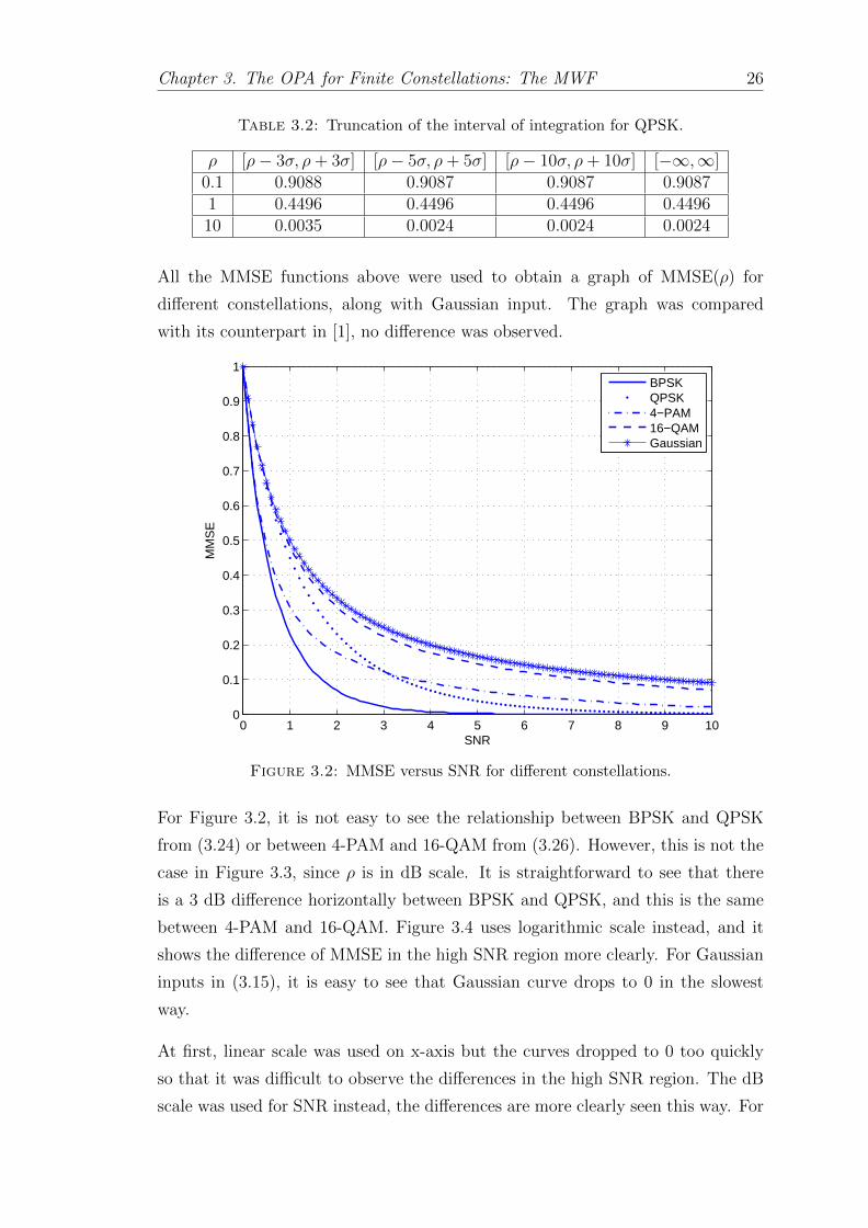
All the MMSE functions above were used to obtain a graph of MMSE(ρ) for
different constellations, along with Gaussian input. The graph was compared
with its counterpart in [1], no difference was observed.
0 1 2 3 4 5 6 7 8 9 100
0.1
0.2
0.3
0.4
0.5
0.6
0.7
0.8
0.9
1
SNR
MM
SE
BPSKQPSK4−PAM16−QAMGaussian
Figure 3.2: MMSE versus SNR for different constellations.
For Figure 3.2, it is not easy to see the relationship between BPSK and QPSK
from (3.24) or between 4-PAM and 16-QAM from (3.26). However, this is not the
case in Figure 3.3, since ρ is in dB scale. It is straightforward to see that there
is a 3 dB difference horizontally between BPSK and QPSK, and this is the same
between 4-PAM and 16-QAM. Figure 3.4 uses logarithmic scale instead, and it
shows the difference of MMSE in the high SNR region more clearly. For Gaussian
inputs in (3.15), it is easy to see that Gaussian curve drops to 0 in the slowest
way.
At first, linear scale was used on x-axis but the curves dropped to 0 too quickly
so that it was difficult to observe the differences in the high SNR region. The dB
scale was used for SNR instead, the differences are more clearly seen this way. For
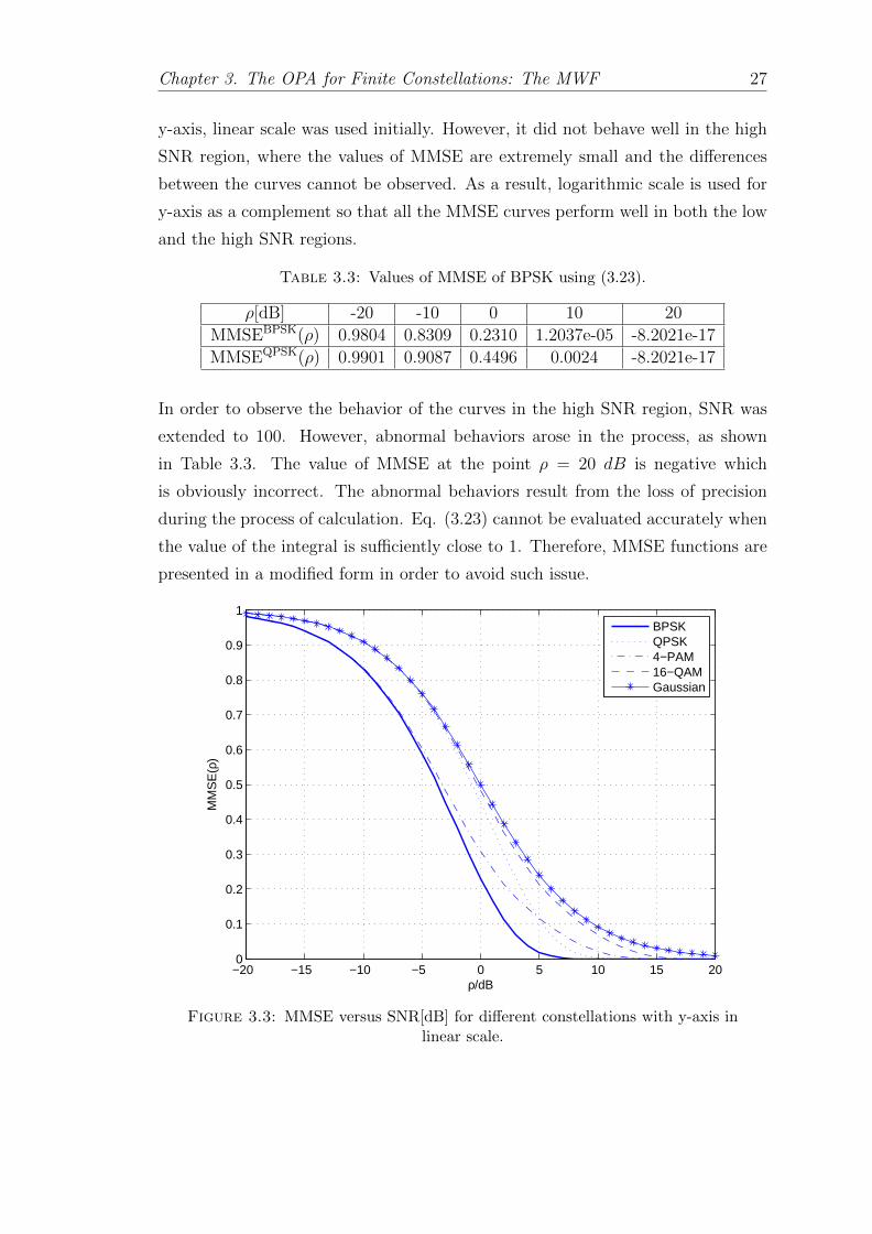
Chapter 3. The OPA for Finite Constellations: The MWF 27
y-axis, linear scale was used initially. However, it did not behave well in the high
SNR region, where the values of MMSE are extremely small and the differences
between the curves cannot be observed. As a result, logarithmic scale is used for
y-axis as a complement so that all the MMSE curves perform well in both the low
and the high SNR regions.
Table 3.3: Values of MMSE of BPSK using (3.23).
ρ[dB] -20 -10 0 10 20
MMSEBPSK(ρ) 0.9804 0.8309 0.2310 1.2037e-05 -8.2021e-17
MMSEQPSK(ρ) 0.9901 0.9087 0.4496 0.0024 -8.2021e-17
In order to observe the behavior of the curves in the high SNR region, SNR was
extended to 100. However, abnormal behaviors arose in the process, as shown
in Table 3.3. The value of MMSE at the point ρ = 20 dB is negative which
is obviously incorrect. The abnormal behaviors result from the loss of precision
during the process of calculation. Eq. (3.23) cannot be evaluated accurately when
the value of the integral is sufficiently close to 1. Therefore, MMSE functions are
presented in a modified form in order to avoid such issue.
−20 −15 −10 −5 0 5 10 15 200
0.1
0.2
0.3
0.4
0.5
0.6
0.7
0.8
0.9
1
ρ/dB
MM
SE
(ρ)
BPSKQPSK4−PAM16−QAMGaussian
Figure 3.3: MMSE versus SNR[dB] for different constellations with y-axis inlinear scale.
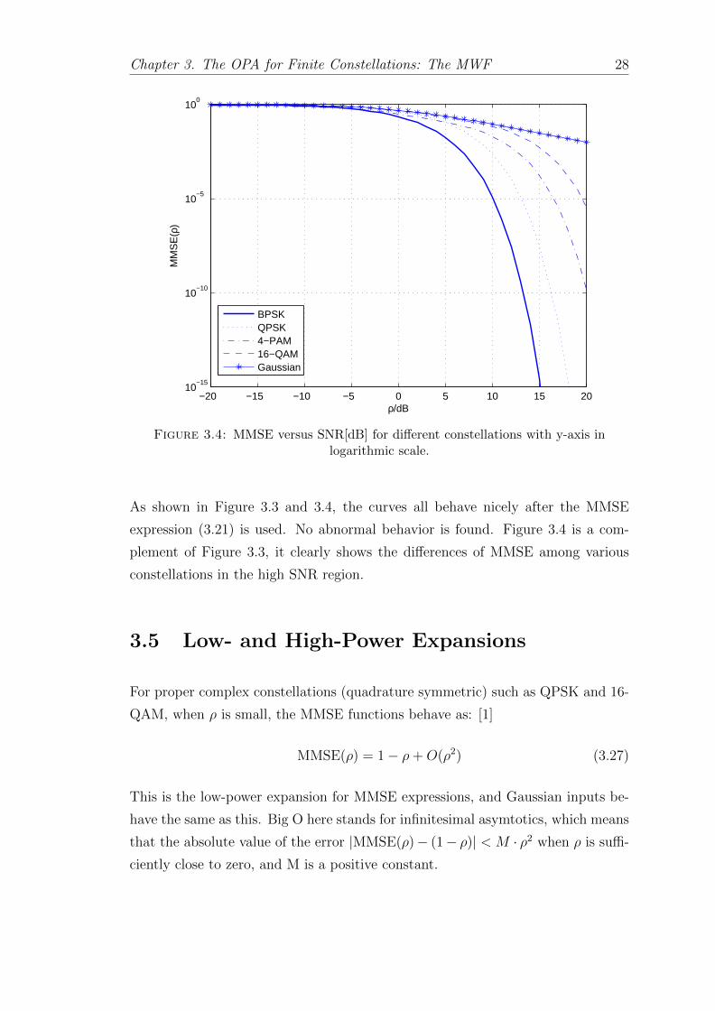
Chapter 3. The OPA for Finite Constellations: The MWF 28
−20 −15 −10 −5 0 5 10 15 2010
−15
10−10
10−5
100
ρ/dB
MM
SE
(ρ)
BPSKQPSK4−PAM16−QAMGaussian
Figure 3.4: MMSE versus SNR[dB] for different constellations with y-axis inlogarithmic scale.
As shown in Figure 3.3 and 3.4, the curves all behave nicely after the MMSE
expression (3.21) is used. No abnormal behavior is found. Figure 3.4 is a com-
plement of Figure 3.3, it clearly shows the differences of MMSE among various
constellations in the high SNR region.
3.5 Low- and High-Power Expansions
For proper complex constellations (quadrature symmetric) such as QPSK and 16-
QAM, when ρ is small, the MMSE functions behave as: [1]
MMSE(ρ) = 1− ρ+O(ρ2) (3.27)
This is the low-power expansion for MMSE expressions, and Gaussian inputs be-
have the same as this. Big O here stands for infinitesimal asymtotics, which means
that the absolute value of the error |MMSE(ρ)− (1− ρ)| < M · ρ2 when ρ is suffi-
ciently close to zero, and M is a positive constant.
Chapter 3. The OPA for Finite Constellations: The MWF 29
On the contrary, for large ρ, Gaussian inputs can be expanded as: [1]
MMSE(ρ) =1
ρ+O(1/ρ2) (3.28)
which is the high-power expansion for Gaussian inputs.
For other constellations, the high-power expansion is mainly decided by the mini-
mum distance defined below:
d = mink 6=l|ck − cl| (3.29)
which can be calculated for M -PAM through (3.19). It is similar to other constel-
lations, and it can be calculated through the power normalization (3.12).
Theorem 3.3. For BPSK and QPSK, the high-power expansion for MMSE(ρ) is:
[1]
MMSE(ρ) =e−
d2
4ρ
d√ρ
(√π +
∞∑l=1
bl(d2ρ)l
)(3.30)
where bl is
bl = (−1)lZ(2l + 1, 1/4)− Z(2l + 1, 3/4)√
π8l×
l∏q=1
(2q − 1) (3.31)
and Z stands for the generalized Rieman Zeta function:
Z(q, ξ) =∞∑k=0
(k + ξ)−q (3.32)
Proof. See Appendix B of [1].
For QPSK, the minimum distance d =√
2. The expansion of (3.30) is truncated
at l = 1. so the high-power expansion above can be written as
MMSE(ρ) =e−
ρ2
√2ρ
(√π − 2.1
ρ
)(3.33)
The derivation of (3.30) can be found in the Appendix A.3.
Chapter 3. The OPA for Finite Constellations: The MWF 30
0 1 2 3 4 5 6 7 8 9 100
0.1
0.2
0.3
0.4
0.5
0.6
0.7
0.8
0.9
1
ρ
MM
SE
(ρ)
QPSKlow−power expansionhigh−power expansion
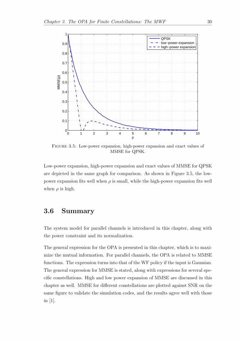
Figure 3.5: Low-power expansion, high-power expansion and exact values ofMMSE for QPSK.
Low-power expansion, high-power expansion and exact values of MMSE for QPSK
are depicted in the same graph for comparison. As shown in Figure 3.5, the low-
power expansion fits well when ρ is small, while the high-power expansion fits well
when ρ is high.
3.6 Summary
The system model for parallel channels is introduced in this chapter, along with
the power constraint and its normalization.
The general expression for the OPA is presented in this chapter, which is to maxi-
mize the mutual information. For parallel channels, the OPA is related to MMSE
functions. The expression turns into that of the WF policy if the input is Gaussian.
The general expression for MMSE is stated, along with expressions for several spe-
cific constellations. High and low power expansion of MMSE are discussed in this
chapter as well. MMSE for different constellations are plotted against SNR on the
same figure to validate the simulation codes, and the results agree well with those
in [1].
Chapter 3. The OPA for Finite Constellations: The MWF 31
Several errors are found in [1], and there are restrictions to some of the figures
in [1] as well. They are discussed in this chapter, and errors are corrected. The
reason of the restriction lies in the structure of the MMSE expression. A loss of
precision is found during the simulation process, it becomes a problem during the
derivation of the OPA in Chapter 4. As a result, MMSE functions are presented
in a modified form to avoid such problem.
Chapter 4
Computation of the OPA
4.1 The Mercury/Waterfilling
The regular waterfilling (WF) policy, which is the OPA with Gaussian inputs, is
discussed above in (3.17) and (3.18). However in the present case, the input dis-
tribution is not Gaussian, and inputs with discrete constellations are used instead
so that the mercury/waterfilling (MWF) policy is introduced in [1][29][30].
The MWF is similar to the regular WF, however the difference is that the MWF
pours ”mercury” first and then ”water”. As discussed in Chapter 2, a new function
Gi(ξ) for arbitrary input distribution is defined as:
Gi(ξ) = 1/ξ −MMSE−1i (ξ), ξ ∈ [0, 1] (4.1)
Gi(ξ) = 1, ξ > 1 (4.2)
As it is shown in (3.16), for Gaussian input, Gi(ξ) = 1 holds for all ξ. For other
inputs with discrete constellations, the MMSE−1(·) for specific constellations are
required in order to obtain Gi(ξ). Using Gi(ξ), the MWF can be presented more
effectively with a few steps, whose graphic interpretation is shown in Figure 2.3.
1. Similar to the regular WF, for all the channels, set up a unit-base vessel solid
up to a height of 1/γi.
2. Determine η, pour mercury into all the vessels until the level of mercury (in-
cluding the solid part) reaches Gi(η/γi)/γi.
32
Chapter 4. Computation of the OPA 33
3. Pour water into all the vessels until the level of water reaches 1/η.
4. The height of water over the mercury is the OPA p∗i for the ith channel.
The MWF is straightforward with all the steps above, and they are only applied to
those channels with η ≤ γi. As for the channels that do not satisfy this inequality,
no mercury is poured into such channels, and the power allocated is zero.
Mercury here serves as an artificial noise to emulate finite constellations. It can
also be interpreted as the gap to the ideal Gaussian input. This approach has an
advantage that it gives an exact OPA for any input constellation instead of just
an approximation. This is why it is called ”exact MWF”.
4.2 Calculating the Water Level 1/η
With everything stated above, the exact MWF OPA for different constellations can
now be calculated if η is known. To compute it, a setting of two parallel channels
is considered first, and then the case of three channels is used for comparison.
For the general case with n parallel channels, (3.14) can be used for the calculation
of the MWF OPA. A special case of two parallel channels is considered in the thesis,
with channel gains γ1 and γ2 respectively (γ1 > γ2). For two parallel channels,
(3.14) can be expressed as:
1
2γ1MMSE−1
(η
γ1
)+
1
2γ2MMSE−1
(η
γ2
)= 1 (4.3)
where γ1 > γ2,ηγ1
< ηγ2
, and since MMSE−1(·) is a monotonically decreasing
function, the following can be obtained:
1
2γ1MMSE−1
(η
γ1
)+
1
2γ2MMSE−1
(η
γ1
)> 1 (4.4)
1
2γ1MMSE−1
(η
γ2
)+
1
2γ2MMSE−1
(η
γ2
)< 1 (4.5)
With inequalities (4.4) and (4.5), upper and lower bounds can be derived for η:
l = γ2MMSE
(2γ1γ2γ1 + γ2
)< η < γ1MMSE
(2γ1γ2γ1 + γ2
)= u (4.6)
Chapter 4. Computation of the OPA 34
In order to calculate η, equation (4.3) has to be solved. The left hand side of (4.3)
is monotonically decreasing, therefore the bisection method can be used to solve
it for η.
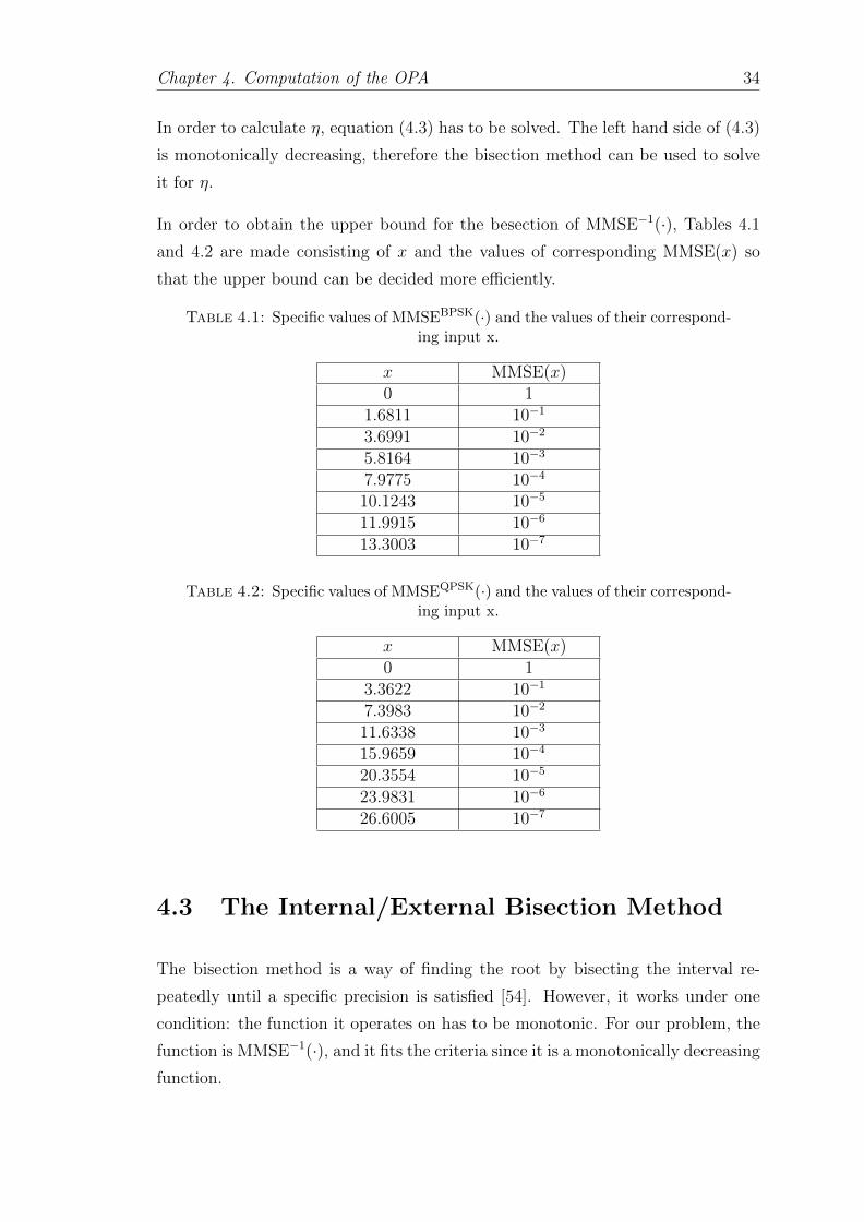
In order to obtain the upper bound for the besection of MMSE−1(·), Tables 4.1
and 4.2 are made consisting of x and the values of corresponding MMSE(x) so
that the upper bound can be decided more efficiently.
Table 4.1: Specific values of MMSEBPSK(·) and the values of their correspond-ing input x.
x MMSE(x)0 1
1.6811 10−1
3.6991 10−2
5.8164 10−3
7.9775 10−4
10.1243 10−5
11.9915 10−6
13.3003 10−7
Table 4.2: Specific values of MMSEQPSK(·) and the values of their correspond-ing input x.
x MMSE(x)0 1
3.3622 10−1
7.3983 10−2
11.6338 10−3
15.9659 10−4
20.3554 10−5
23.9831 10−6
26.6005 10−7
4.3 The Internal/External Bisection Method
The bisection method is a way of finding the root by bisecting the interval re-
peatedly until a specific precision is satisfied [54]. However, it works under one
condition: the function it operates on has to be monotonic. For our problem, the
function is MMSE−1(·), and it fits the criteria since it is a monotonically decreasing
function.
Chapter 4. Computation of the OPA 35
The bisection method is simple and robust. In our case, it takes more time to pro-
cess due to the internal and external bisections required. For the present problem,
the upper and lower bounds derived for η result in a reasonable running time of
codes, since the bounds are quite tight.
A new function is formed based on (4.3):
f(η) =1
2γ1MMSE−1
(η
γ1
)+
1
2γ2MMSE−1
(η
γ2
)− 1 (4.7)
First, with the upper and lower bounds from (4.6), a middle point was calculated
to beγ1 + γ2
2MMSE
(2γ1γ2γ1 + γ2
). It is substituted into (4.7) to compute the value
of f(η) and compare with 0.
On the other hand, there are two MMSE−1(·) in (4.3) which means two inter-
nal bisections are needed. They have to be calculated by inverting MMSE func-
tions using the bisection method as well, since there is no explicit expression for
MMSE−1(·) for any constellation.
Consider ρi = MMSE−1i
(ηγi
), and a new function is formed:
fi(ρi) = MMSEi(ρi)−η
γi, i = 1, ..., n (4.8)
where n = 2 in this case.
In order to calculate MMSE−1(·) through bisection, an upper bound is needed for
ρi. The upper bound for ρi can be determined as long as it satisfies the inequality
MMSEi(ρupperi ) <
ηlowerγ1
.
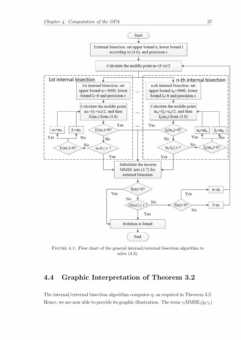
An algorithm of obtaining the MWF OPA is developed based on the bisection
method. Its specific steps are presented as follows, along with an intuitive flow
chart shown in Figure 4.1.
1. Set an upper bound u and a lower bound l for η for external bisection according
to (4.6).
2. Compute the middle point m =l + u
2.
Chapter 4. Computation of the OPA 36
3. For the internal bisection, set the lower bound of ρi to be li = 0 since
MMSE−1(·) ∈ [0,∞), and set the upper bound of ρi for BPSK and QPSK accord-
ing to Table 4.1 and 4.2. In our case 1, the upper bound is set to be ui = 3000, so
that it satisfies:
MMSEi(ρupper) ≤ηlowerγ1
=γ2γ1
MMSE
(2γ1γ2γ1 + γ2
)(4.9)
4. The middle point for the internal bisection is mi =ui + li
2. Compute fi(mi)
and compare with 0. If fi(mi) = 0, then ρi = mi. Else, set the new upper bound
to be ui = mi if fi(mi) < 0, otherwise set the new lower bound to be li = mi.
5. Repeat step 4 until ui− li ≤ ε is fit and ρi = mi, where ε is the precision of the
internal bisection.
6. Substitute ρi that obtained from step 3 into (4.7) for the external bisection. If
f(m) = 0, then η = m. Else, set the new upper bound to be u = m if f(m) < 0,
otherwise set the new lower bound to be l = m.
7. Repeat step 2-6 until |f(m)| ≤ ε is fit and η = m, where ε is the precision of
the external bisection.
However, an issue emerged when using Matlab to program MMSE functions. Ex-
pression (3.22) was used to evaluate MMSE functions initially, but a loss of pre-
cision was found. The curve was not monotonic anymore when ρ was high. It
was realized that the problem lied in the structure of the expression. Numerical
computation is not sufficiently accurate when the value of the integral in (3.22) is
extremely close to 1. There was a loss of precision in the process of calculation.
As a result, expression (3.21) was used instead. This issue occurred several times,
which is discussed thoroughly in the subsequent chapters.
1QPSK, 16-QAM, 64-QAM and 256-QAM inputs with channel gains |h1|2 = 2|h2|2,|h1|2 =10|h2|2 and |h1|2 = 100|h2|2 are considered in the thesis.
Chapter 4. Computation of the OPA 37
Figure 4.1: Flow chart of the general internal/external bisection algorithm tosolve (4.3).
4.4 Graphic Interpretation of Theorem 3.2
The internal/external bisection algorithm computes η, as required in Theorem 3.2.
Hence, we are now able to provide its graphic illustration. The term γiMMSEi(piγi)
Chapter 4. Computation of the OPA 38
is plotted versus pi. A horizontal line y=η is drawn as well, where η is solved
using the bisection method mentioned above. According to Theorem 3.2, it is
straightforward to see that the intersections between curves, and the horizontal
line correspond to the OPA.
Three different scenarios are considered:
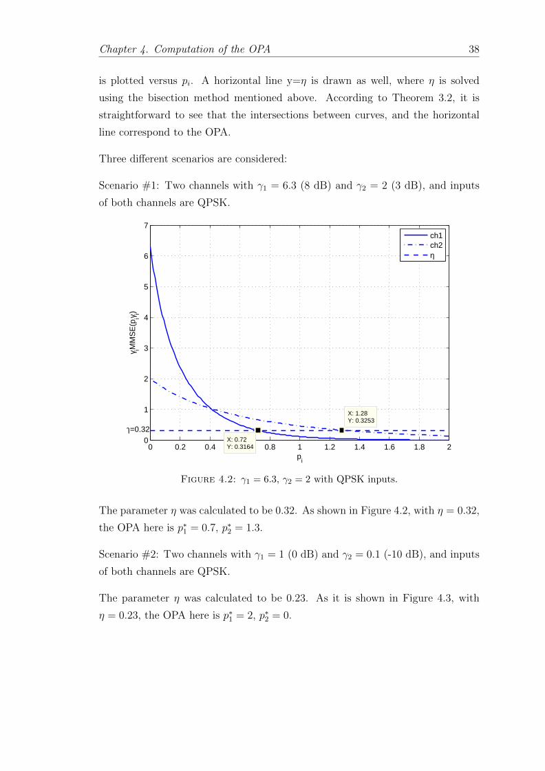
Scenario #1: Two channels with γ1 = 6.3 (8 dB) and γ2 = 2 (3 dB), and inputs
of both channels are QPSK.
0 0.2 0.4 0.6 0.8 1 1.2 1.4 1.6 1.8 20
1
2
3
4
5
6
7
X: 0.72Y: 0.3164
pi
γ iMM
SE
(piγ i)
X: 1.28Y: 0.3253
ch1ch2η
η=0.32
Figure 4.2: γ1 = 6.3, γ2 = 2 with QPSK inputs.
The parameter η was calculated to be 0.32. As shown in Figure 4.2, with η = 0.32,
the OPA here is p∗1 = 0.7, p∗2 = 1.3.
Scenario #2: Two channels with γ1 = 1 (0 dB) and γ2 = 0.1 (-10 dB), and inputs
of both channels are QPSK.
The parameter η was calculated to be 0.23. As it is shown in Figure 4.3, with
η = 0.23, the OPA here is p∗1 = 2, p∗2 = 0.
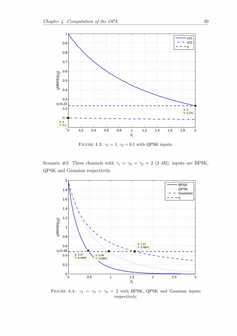
Chapter 4. Computation of the OPA 39
0 0.2 0.4 0.6 0.8 1 1.2 1.4 1.6 1.8 20
0.1
0.2
0.3
0.4
0.5
0.6
0.7
0.8
0.9
1
X: 0Y: 0.1
pi
γ iMM
SE
(piγ i)
X: 2Y: 0.231
ch1ch2η
η=0.23
Figure 4.3: γ1 = 1, γ2 = 0.1 with QPSK inputs.
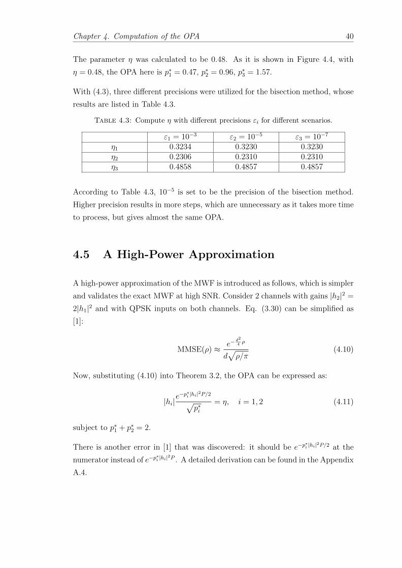
Scenario #3: Three channels with γ1 = γ2 = γ3 = 2 (3 dB), inputs are BPSK,
QPSK and Gaussian respectively.
0 0.5 1 1.5 2 2.5 30
0.2
0.4
0.6
0.8
1
1.2
1.4
1.6
1.8
2
X: 0.47Y: 0.4989
pi
γ iMM
SE
(piγ i)
X: 0.96Y: 0.4863
X: 1.57Y: 0.4831
BPSKQPSKGaussianη
η=0.48
Figure 4.4: γ1 = γ2 = γ3 = 2 with BPSK, QPSK and Gaussian inputsrespectively.
Chapter 4. Computation of the OPA 40
The parameter η was calculated to be 0.48. As it is shown in Figure 4.4, with
η = 0.48, the OPA here is p∗1 = 0.47, p∗2 = 0.96, p∗3 = 1.57.
With (4.3), three different precisions were utilized for the bisection method, whose
results are listed in Table 4.3.
Table 4.3: Compute η with different precisions εi for different scenarios.
ε1 = 10−3 ε2 = 10−5 ε3 = 10−7
η1 0.3234 0.3230 0.3230η2 0.2306 0.2310 0.2310η3 0.4858 0.4857 0.4857
According to Table 4.3, 10−5 is set to be the precision of the bisection method.
Higher precision results in more steps, which are unnecessary as it takes more time
to process, but gives almost the same OPA.
4.5 A High-Power Approximation
A high-power approximation of the MWF is introduced as follows, which is simpler
and validates the exact MWF at high SNR. Consider 2 channels with gains |h2|2 =
2|h1|2 and with QPSK inputs on both channels. Eq. (3.30) can be simplified as
[1]:
MMSE(ρ) ≈ e−d2
4ρ
d√ρ/π
(4.10)
Now, substituting (4.10) into Theorem 3.2, the OPA can be expressed as:
|hi|e−p
∗i |hi|2P/2√p∗i
= η, i = 1, 2 (4.11)
subject to p∗1 + p∗2 = 2.
There is another error in [1] that was discovered: it should be e−p∗i |hi|2P/2 at the
numerator instead of e−p∗i |hi|2P . A detailed derivation can be found in the Appendix
A.4.
Chapter 4. Computation of the OPA 41
Using (4.11), the following equation can be derived:
γ1e−
12p∗1γ1√
2p∗1γ1/π= γ2
e−12p∗2γ2√
2p∗2γ2/π(4.12)
where γ2 = 2γ1 holds, since |h2|2 = 2|h1|2 and γi = P |hi|2. The equation can be
further simplified as
e−p∗1γ1
p∗1=
2e−2(2−p∗1)γ1
2− p∗1(4.13)
with p∗1 + p∗2 = 2. From (4.13), the following function can be formed:
F (p∗1) =e−p
∗1γ1
p∗1− 2e−2(2−p
∗1)γ1
2− p∗1(4.14)
The terms e−p∗i γi and (2 − p∗1) decreases with p∗1. On the contrary, 2e−2(2−p
∗1)γi
increases with p∗1. As a result, the first term of (4.14) decreases with p∗1, and
the second term2e−2(2−p
∗1)γ1
2− p∗1increases with p∗1. Overall, F (p∗1) is a monotonically
decreasing function of p∗1, so that the bisection method can be utilized to solve
F (p∗1) = 0 for p∗i .
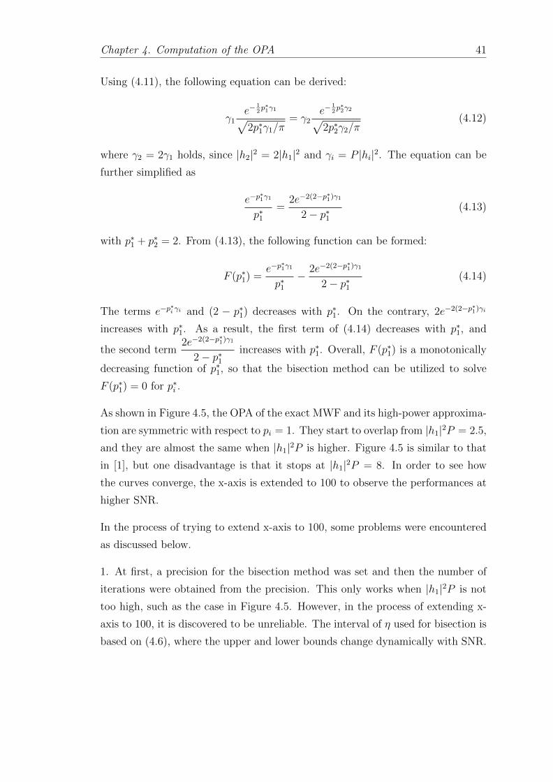
As shown in Figure 4.5, the OPA of the exact MWF and its high-power approxima-
tion are symmetric with respect to pi = 1. They start to overlap from |h1|2P = 2.5,
and they are almost the same when |h1|2P is higher. Figure 4.5 is similar to that
in [1], but one disadvantage is that it stops at |h1|2P = 8. In order to see how
the curves converge, the x-axis is extended to 100 to observe the performances at
higher SNR.
In the process of trying to extend x-axis to 100, some problems were encountered
as discussed below.
1. At first, a precision for the bisection method was set and then the number of
iterations were obtained from the precision. This only works when |h1|2P is not
too high, such as the case in Figure 4.5. However, in the process of extending x-
axis to 100, it is discovered to be unreliable. The interval of η used for bisection is
based on (4.6), where the upper and lower bounds change dynamically with SNR.
Chapter 4. Computation of the OPA 42
0 1 2 3 4 5 6 7 80
0.2
0.4
0.6
0.8
1
1.2
1.4
1.6
1.8
2
hi2*P
p i
Ch2
Ch2
Ch1
Ch1
Exact mercury/waterfillingHigh−power Approximation
Figure 4.5: Power allocation for two channels with |h2|2 = 2|h1|2, both withQPSK inputs, versus |h1|2P .
The number of iterations for bisection, k, is determined by the range as follows:
k =
⌈log2
(u− lε
)⌉(4.15)
where u is the upper bound of η, l is the lower bound of η, ε is the precision of
the external bisection method.
The number of iterations k shrinks as the range u− l becomes smaller, and even-
tually turns into 1, which is insufficient for the bisection method to find the root.
Therefore k is set to be 20, and the stopping criteria for the bisection method in
this case is:
|f(η)| =∣∣∣∣ 1
2γ1MMSE−1
(η
γ1
)+
1
2γ2MMSE−1
(η
γ2
)− 1
∣∣∣∣ < ε = 10−3 (4.16)
Chapter 4. Computation of the OPA 43
−20 −15 −10 −5 0 5 10 15 200
0.2
0.4
0.6
0.8
1
1.2
1.4
1.6
1.8
2
SNR/dB
p i
Ch1
Ch2
Exact mercury/waterfilling
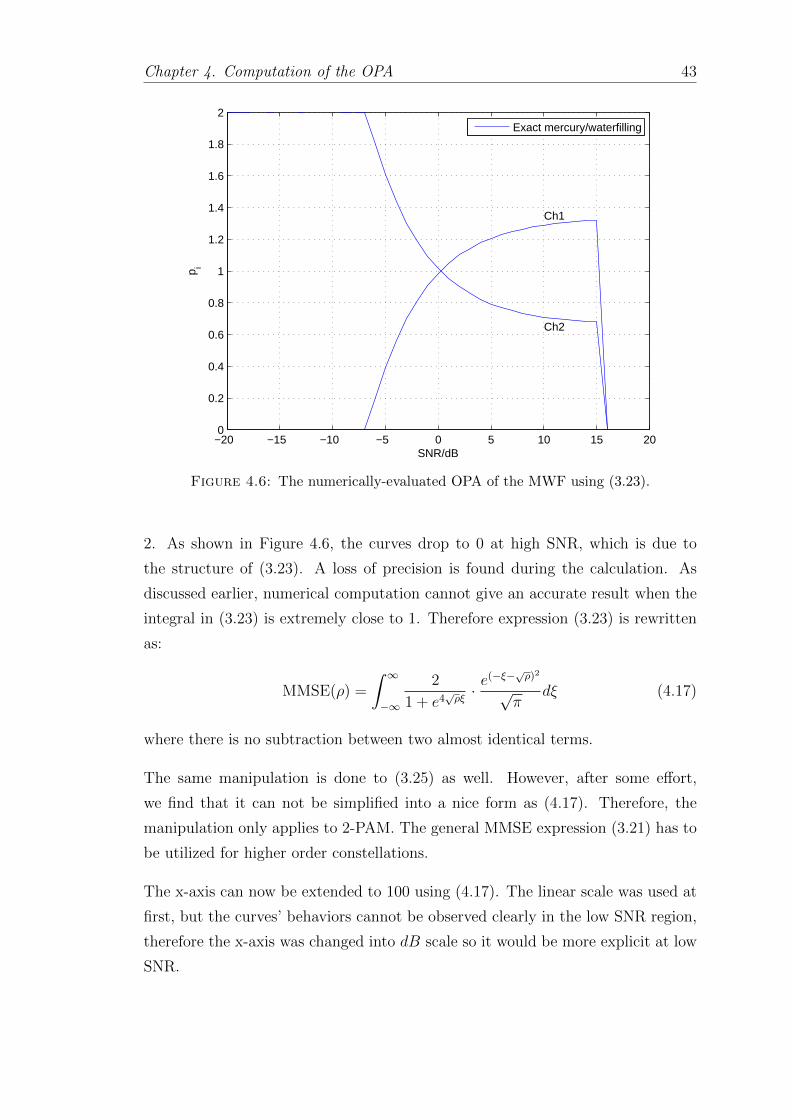
Figure 4.6: The numerically-evaluated OPA of the MWF using (3.23).
2. As shown in Figure 4.6, the curves drop to 0 at high SNR, which is due to
the structure of (3.23). A loss of precision is found during the calculation. As
discussed earlier, numerical computation cannot give an accurate result when the
integral in (3.23) is extremely close to 1. Therefore expression (3.23) is rewritten
as:
MMSE(ρ) =
∫ ∞−∞
2
1 + e4√ρξ· e
(−ξ−√ρ)2
√π
dξ (4.17)
where there is no subtraction between two almost identical terms.
The same manipulation is done to (3.25) as well. However, after some effort,
we find that it can not be simplified into a nice form as (4.17). Therefore, the
manipulation only applies to 2-PAM. The general MMSE expression (3.21) has to
be utilized for higher order constellations.
The x-axis can now be extended to 100 using (4.17). The linear scale was used at
first, but the curves’ behaviors cannot be observed clearly in the low SNR region,
therefore the x-axis was changed into dB scale so it would be more explicit at low
SNR.
Chapter 4. Computation of the OPA 44
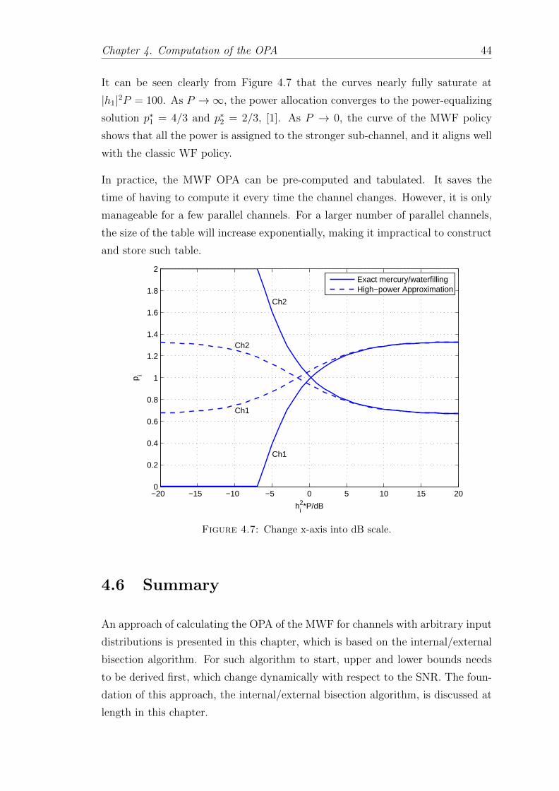
It can be seen clearly from Figure 4.7 that the curves nearly fully saturate at
|h1|2P = 100. As P →∞, the power allocation converges to the power-equalizing
solution p∗1 = 4/3 and p∗2 = 2/3, [1]. As P → 0, the curve of the MWF policy
shows that all the power is assigned to the stronger sub-channel, and it aligns well
with the classic WF policy.
In practice, the MWF OPA can be pre-computed and tabulated. It saves the
time of having to compute it every time the channel changes. However, it is only
manageable for a few parallel channels. For a larger number of parallel channels,
the size of the table will increase exponentially, making it impractical to construct
and store such table.
−20 −15 −10 −5 0 5 10 15 200
0.2
0.4
0.6
0.8
1
1.2
1.4
1.6
1.8
2
hi2*P/dB
p i
Ch2
Ch2
Ch1
Ch1
Exact mercury/waterfillingHigh−power Approximation
Figure 4.7: Change x-axis into dB scale.
4.6 Summary
An approach of calculating the OPA of the MWF for channels with arbitrary input
distributions is presented in this chapter, which is based on the internal/external
bisection algorithm. For such algorithm to start, upper and lower bounds needs
to be derived first, which change dynamically with respect to the SNR. The foun-
dation of this approach, the internal/external bisection algorithm, is discussed at
length in this chapter.
Chapter 4. Computation of the OPA 45
A graphic interpretation of how to obtain the OPA is presented, and several sce-
narios are considered with different channel gains and different constellations. Cal-
culation of the OPA becomes a straightforward numerical task.
A high-power approximation is derived using the high-power expansion of MMSE
functions from the last chapter. Once its OPA is derived, they are substituted
into the expression of constellation capacity in [13]. High-power approximation is
plotted in the same figure for comparison. It fits well with the MWF in the high
SNR region.
The restrictions discussed in the last chapter occur here. The curves all drop to
zero when the SNR is extended to 100. Specific MMSE expressions for different
constellations were used at first, and then it was realized that the problem was
their structure. The general MMSE expression (3.21) was used instead and then
SNR can be extended to 100 without any abnormal behavior.
Chapter 5
Approximations of the
Constellation Capacity
5.1 The Constellation-Constrained Capacity
Consider a communication system with n parallel channels (as shown in Figure
3.1) with Gaussian inputs, the channel capacity is,
C =1
2log2(1 + ρ) (5.1)
where ρ is the SNR of the channel.
In practice, discrete alphabets are utilized to transmit information efficiently.
Those discrete alphabets are formed into constellations. The maximum reliable
transmission rate available with a given constellation is the constellation capacity.
It is lower than the channel capacity C and upper-bounded by the modulation
alphabet entropy [14]:
CM ≤ min(C, log2M) (5.2)
where M is the constellation cardinality.
For M -PAM, the constellation points can be found through power constraint in
(3.2). The distance between two constellation points is:
dij = ci − cj (5.3)
46
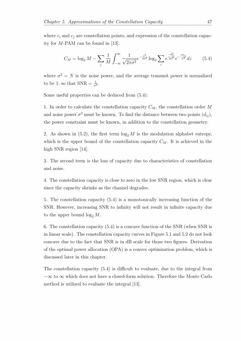
Chapter 5. Approximations of the Constellation Capacity 47
where ci and cj are constellation points, and expression of the constellation capac-
ity for M -PAM can be found in [13]:
CM = log2M −∑j
1
M
∫ ∞−∞
1√2πσ2
e−z2
2σ2 log2
∑i
e−d2ij2σ2 e−
zdij
σ2 dz (5.4)
where σ2 = N is the noise power, and the average transmit power is normalized
to be 1, so that SNR = 1σ2 .
Some useful properties can be deduced from (5.4):
1. In order to calculate the constellation capacity CM , the constellation order M
and noise power σ2 must be known. To find the distance between two points (dij),
the power constraint must be known, in addition to the constellation geometry.
2. As shown in (5.2), the first term log2M is the modulation alphabet entropy,
which is the upper bound of the constellation capacity CM . It is achieved in the
high SNR region [14].
3. The second term is the loss of capacity due to characteristics of constellation
and noise.
4. The constellation capacity is close to zero in the low SNR region, which is clear
since the capacity shrinks as the channel degrades.
5. The constellation capacity (5.4) is a monotonically increasing function of the
SNR. However, increasing SNR to infinity will not result in infinite capacity due
to the upper bound log2M .
6. The constellation capacity (5.4) is a concave function of the SNR (when SNR is
in linear scale). The constellation capacity curves in Figure 5.1 and 5.2 do not look
concave due to the fact that SNR is in dB scale for those two figures. Derivation
of the optimal power allocation (OPA) is a convex optimization problem, which is
discussed later in this chapter.
The constellation capacity (5.4) is difficult to evaluate, due to the integral from
−∞ to∞ which does not have a closed-form solution. Therefore the Monte Carlo
method is utilized to evaluate the integral [13].
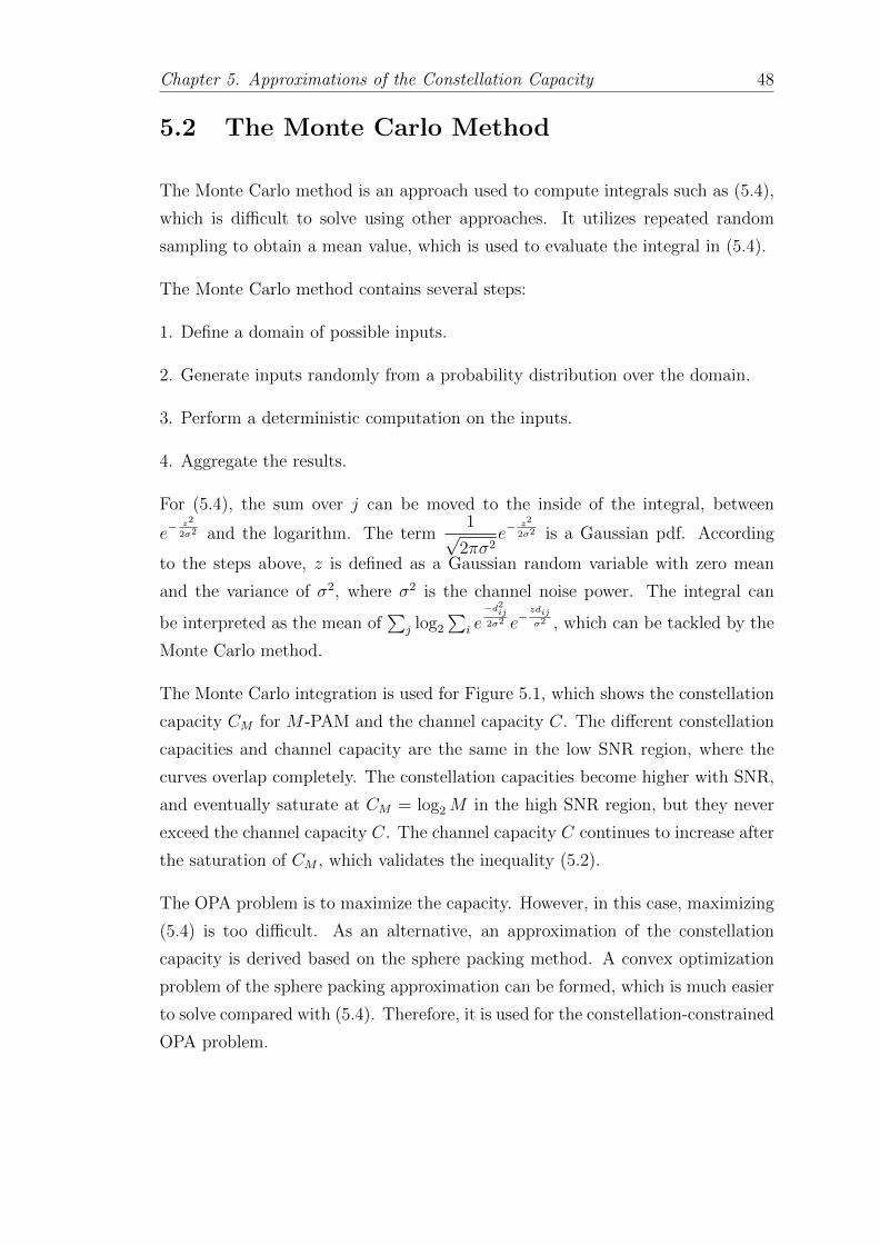
Chapter 5. Approximations of the Constellation Capacity 48
5.2 The Monte Carlo Method
The Monte Carlo method is an approach used to compute integrals such as (5.4),
which is difficult to solve using other approaches. It utilizes repeated random
sampling to obtain a mean value, which is used to evaluate the integral in (5.4).
The Monte Carlo method contains several steps:
1. Define a domain of possible inputs.
2. Generate inputs randomly from a probability distribution over the domain.
3. Perform a deterministic computation on the inputs.
4. Aggregate the results.
For (5.4), the sum over j can be moved to the inside of the integral, between
e−z2
2σ2 and the logarithm. The term1√
2πσ2e−
z2
2σ2 is a Gaussian pdf. According
to the steps above, z is defined as a Gaussian random variable with zero mean
and the variance of σ2, where σ2 is the channel noise power. The integral can
be interpreted as the mean of∑
j log2
∑i e
−d2ij2σ2 e−
zdij
σ2 , which can be tackled by the
Monte Carlo method.
The Monte Carlo integration is used for Figure 5.1, which shows the constellation
capacity CM for M -PAM and the channel capacity C. The different constellation
capacities and channel capacity are the same in the low SNR region, where the
curves overlap completely. The constellation capacities become higher with SNR,
and eventually saturate at CM = log2M in the high SNR region, but they never
exceed the channel capacity C. The channel capacity C continues to increase after
the saturation of CM , which validates the inequality (5.2).
The OPA problem is to maximize the capacity. However, in this case, maximizing
(5.4) is too difficult. As an alternative, an approximation of the constellation
capacity is derived based on the sphere packing method. A convex optimization
problem of the sphere packing approximation can be formed, which is much easier
to solve compared with (5.4). Therefore, it is used for the constellation-constrained
OPA problem.
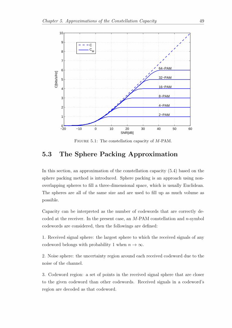
Chapter 5. Approximations of the Constellation Capacity 49
−20 −10 0 10 20 30 40 50 600
1
2
3
4
5
6
7
8
9
10
SNR[dB]
C[b
its/s
/Hz]
2−PAM
4−PAM
8−PAM
16−PAM
32−PAM
64−PAM
CC
M
Figure 5.1: The constellation capacity of M -PAM.
5.3 The Sphere Packing Approximation
In this section, an approximation of the constellation capacity (5.4) based on the
sphere packing method is introduced. Sphere packing is an approach using non-
overlapping spheres to fill a three-dimensional space, which is usually Euclidean.
The spheres are all of the same size and are used to fill up as much volume as
possible.
Capacity can be interpreted as the number of codewords that are correctly de-
coded at the receiver. In the present case, an M -PAM constellation and n-symbol
codewords are considered, then the followings are defined:
1. Received signal sphere: the largest sphere to which the received signals of any
codeword belongs with probability 1 when n→∞.
2. Noise sphere: the uncertainty region around each received codeword due to the
noise of the channel.
3. Codeword region: a set of points in the received signal sphere that are closer
to the given codeword than other codewords. Received signals in a codeword’s
region are decoded as that codeword.
Chapter 5. Approximations of the Constellation Capacity 50
For n-symbol codewords, the received signal sphere has a radius of√nP , where P
is the maximum power of each independent symbol. Any point within this sphere
can be an eligible codeword, which can be decoded correctly at the receiver as long
as there is no channel noise.
However, channel noise is inevitable. The noise sphere of the codeword has a
radius of√nσ2, where σ2 is the average noise power per symbol. The codewords
cannot be selected too closely to each other, in which case their noise sphere will
be overlapped and the receiver is unable to decode them correctly. As a result,
the number of distinct codewords is the number of non-overlapping noise spheres
that can fit in the received signal sphere [3] [14].
N =α(√nP + nσ2)n
α(√nσ2)n
= (1 + ρ)n/2 (5.5)
where α is
α =πn/2
Γ(n2
+ 1) (5.6)
where Γ is the gamma function. If P is a constant, the number of distinct code-
words N decreases as noise power σ2 increases. In this case, the channel capacity
can be calculated as:
C =1
nlog2N =
1
2log2(1 + ρ) (5.7)
However, once a specific constellation is applied, the number of codewords turns
into Mn. Constellation geometry has to be taken into account when choosing the
codewords. The minimum distance constraint between the constellation points
has an influence on how the received signal sphere is arranged.
Due to the minimum distance constraint, the receiver can decode all the codewords
correctly if the noise power σ2 is sufficiently small. In this case, the received signal
sphere has a radius of√nP + nσ2 ≈
√nP , therefore its volume is
V = α(√nP )n (5.8)
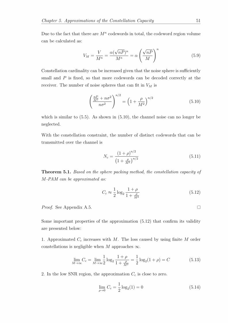
Chapter 5. Approximations of the Constellation Capacity 51
Due to the fact that there are Mn codewords in total, the codeword region volume
can be calculated as:
VM =V
Mn=α(√nP )n
Mn= α
(√nP
M
)n
(5.9)
Constellation cardinality can be increased given that the noise sphere is sufficiently
small and P is fixed, so that more codewords can be decoded correctly at the
receiver. The number of noise spheres that can fit in VM is(nPM2 + nσ2
nσ2
)n/2
=(
1 +ρ
M2
)n/2(5.10)
which is similar to (5.5). As shown in (5.10), the channel noise can no longer be
neglected.
With the constellation constraint, the number of distinct codewords that can be
transmitted over the channel is
Nc =(1 + ρ)n/2(1 + ρ
M2
)n/2 (5.11)
Theorem 5.1. Based on the sphere packing method, the constellation capacity of
M-PAM can be approximated as:
Cc ≈1
2log2
1 + ρ
1 + ρM2
(5.12)
Proof. See Appendix A.5.
Some important properties of the approximation (5.12) that confirm its validity
are presented below:
1. Approximated Cc increases with M . The loss caused by using finite M order
constellations is negligible when M approaches ∞.
limM→∞
Cc = limM→∞
1
2log2
1 + ρ
1 + ρM2
=1
2log2(1 + ρ) = C (5.13)
2. In the low SNR region, the approximation Cc is close to zero.
limρ→0
Cc =1
2log2(1) = 0 (5.14)
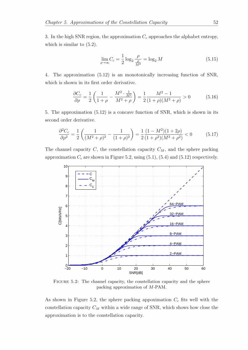
Chapter 5. Approximations of the Constellation Capacity 52
3. In the high SNR region, the approximation Cc approaches the alphabet entropy,
which is similar to (5.2).
limρ→∞
Cc =1
2log2
ρρM2
= log2M (5.15)
4. The approximation (5.12) is an monotonically increasing function of SNR,
which is shown in its first order derivative.
∂Cc∂ρ
=1
2
(1
1 + ρ−M2 · 1
M2
M2 + ρ
)=
1
2
M2 − 1
(1 + ρ)(M2 + ρ)> 0 (5.16)
5. The approximation (5.12) is a concave function of SNR, which is shown in its
second order derivative.
∂2Cc∂ρ2
=1
2
(1
(M2 + ρ)2− 1
(1 + ρ)2
)=
1
2
(1−M2)(1 + 2ρ)
(1 + ρ2)(M2 + ρ2)< 0 (5.17)
The channel capacity C, the constellation capacity CM , and the sphere packing
approximation Cc are shown in Figure 5.2, using (5.1), (5.4) and (5.12) respectively.
−20 −10 0 10 20 30 40 50 600
1
2
3
4
5
6
7
8
9
10
SNR[dB]
C[b
its/s
/Hz]
2−PAM
4−PAM
8−PAM
16−PAM
32−PAM
64−PAM
CC
M
CC
Figure 5.2: The channel capacity, the constellation capacity and the spherepacking approximation of M -PAM.
As shown in Figure 5.2, the sphere packing appoximation Cc fits well with the
constellation capacity CM within a wide range of SNR, which shows how close the
approximation is to the constellation capacity.
Chapter 5. Approximations of the Constellation Capacity 53
For M -QAM, it can be considered as two√M -PAM in quadrature, each with half
the power of M -QAM. Therefore the sphere packing approximation for M -QAM
can be written as
Cc = 2 · 1
2log2
1 + ρ
1 + ρ
(√M)2
= log2
1 + ρ
1 + ρM
(5.18)
In conclusion, the sphere packing approximation is a good fit for the constellation-
constrained capacity. It is a closed-form expression which is a better objective
function for convex optimization compared with the constellation capacity (5.4).
The sphere packing approximation also retains the key properties of the constel-
lation capacity. This approximation is utilized to obtain the OPA for parellel
channels under a total power constraint and a constellation constraint in the next
section.
5.4 The Constellation-Constrained Waterfilling
For M -QAM, an expression of the constellation capacity can be derived from (5.4).
For n parallel channels, it can be written as:
CM =n∑k=1
(log2Mk −
∑j
1√Mk
∫ ∞−∞
1√2πσ2
k
e− z2
2σ2k log2
∑i
e
−d2ij2σ2k e−zdij
σ2k dz
)(5.19)
where Mk is the constellation order on kth channel, and σ2k is the noise power on
kth channel. The notations in this section are from [2], which are only used in this
chapter for results validation.
In this case, the SNR is defined as:
ρk =gkpkσ2
(5.20)
where gk is the power gain of the kth channel, pk is the power allocated to channel
k, and the total power constraint is∑n
k=1 pk = PT .
Chapter 5. Approximations of the Constellation Capacity 54
The sphere packing approximation of M -QAM (5.18) can be used to obtain an
approximation for (5.19):
Cc =n∑k=1
(log2(1 + gkpk)− log2
(1 +
gkpkMk
))(5.21)
Capacity needs to be maximized in order to obtain the OPA, so that the opti-
mization problem can be written as follows:
max∑k
log2
1 + gkpk1 + gkpk
Mk
(5.22)
s.t.∑k
pk ≤ PT , pk ≥ 0 for all k (5.23)
Theorem 5.2. The OPA for the optimization problem above is:
pk =1
2gk
(√(Mk − 1)2 +
4gkλ
(Mk − 1)− (Mk + 1)
), gk > λ
(1− 1
Mk
)−1(5.24)
pk = 0, gk ≤ λ
(1− 1
Mk
)−1(5.25)
where λ is the Lagrangian multiplier for total power constraint∑
k pk = PT , and
λ ≥ 0.
Proof. See Appendix A.6.
This OPA scheme is unique, since the objective function is strictly concave. De-
tailed derivation of Theorem 5.2 is presented in the Appendix A.6.
Theorem 5.2 turns into the regular waterfilling (WF) policy when M →∞:
limM→∞
pk = 0, gk ≤ λ (5.26)
limM→∞
pk = − 1
gk+
1
λ, gk > λ (5.27)
The derivation of the regular WF from Theorem 5.2 when M →∞ can be found
in the Appendix A.7.
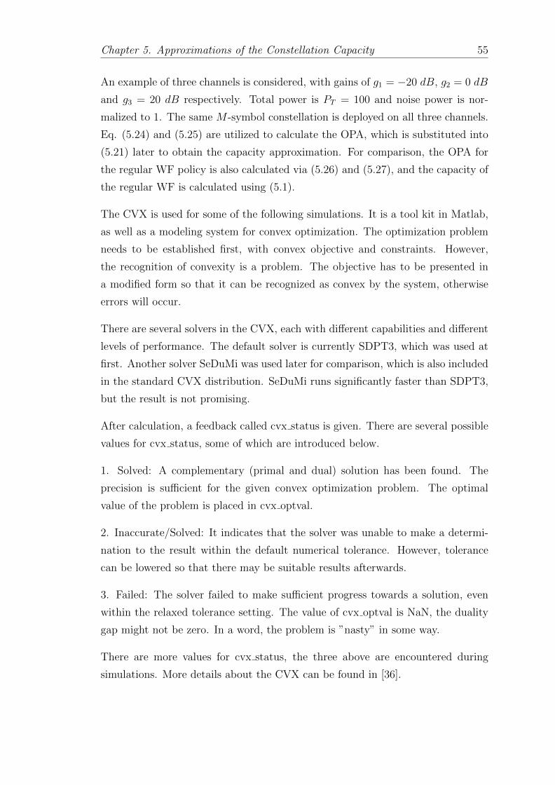
Chapter 5. Approximations of the Constellation Capacity 55
An example of three channels is considered, with gains of g1 = −20 dB, g2 = 0 dB
and g3 = 20 dB respectively. Total power is PT = 100 and noise power is nor-
malized to 1. The same M -symbol constellation is deployed on all three channels.
Eq. (5.24) and (5.25) are utilized to calculate the OPA, which is substituted into
(5.21) later to obtain the capacity approximation. For comparison, the OPA for
the regular WF policy is also calculated via (5.26) and (5.27), and the capacity of
the regular WF is calculated using (5.1).
The CVX is used for some of the following simulations. It is a tool kit in Matlab,
as well as a modeling system for convex optimization. The optimization problem
needs to be established first, with convex objective and constraints. However,
the recognition of convexity is a problem. The objective has to be presented in
a modified form so that it can be recognized as convex by the system, otherwise
errors will occur.
There are several solvers in the CVX, each with different capabilities and different
levels of performance. The default solver is currently SDPT3, which was used at
first. Another solver SeDuMi was used later for comparison, which is also included
in the standard CVX distribution. SeDuMi runs significantly faster than SDPT3,
but the result is not promising.
After calculation, a feedback called cvx status is given. There are several possible
values for cvx status, some of which are introduced below.
1. Solved: A complementary (primal and dual) solution has been found. The
precision is sufficient for the given convex optimization problem. The optimal
value of the problem is placed in cvx optval.
2. Inaccurate/Solved: It indicates that the solver was unable to make a determi-
nation to the result within the default numerical tolerance. However, tolerance
can be lowered so that there may be suitable results afterwards.
3. Failed: The solver failed to make sufficient progress towards a solution, even
within the relaxed tolerance setting. The value of cvx optval is NaN, the duality
gap might not be zero. In a word, the problem is ”nasty” in some way.
There are more values for cvx status, the three above are encountered during
simulations. More details about the CVX can be found in [36].
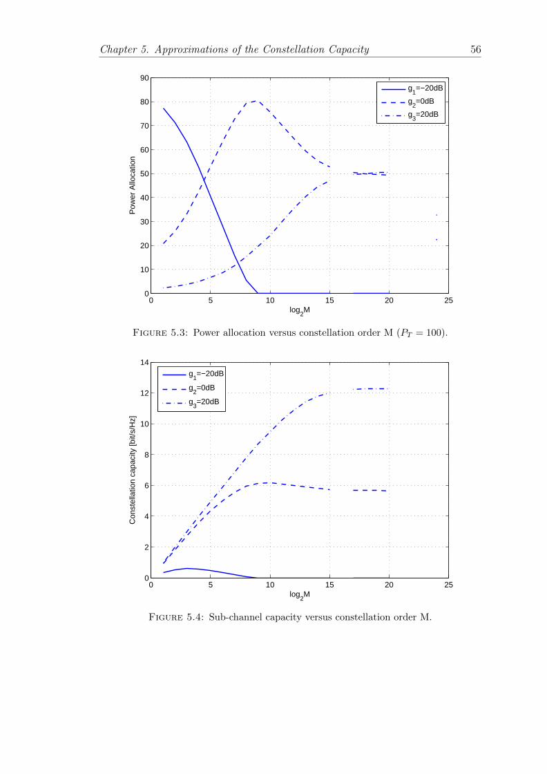
Chapter 5. Approximations of the Constellation Capacity 56
0 5 10 15 20 250
10
20
30
40
50
60
70
80
90
log2M
Pow
er A
lloca
tion
g
1=−20dB
g2=0dB
g3=20dB
Figure 5.3: Power allocation versus constellation order M (PT = 100).
0 5 10 15 20 250
2
4
6
8
10
12
14
log2M
Con
stel
latio
n ca
paci
ty [b
it/s/
Hz]
g
1=−20dB
g2=0dB
g3=20dB
Figure 5.4: Sub-channel capacity versus constellation order M.
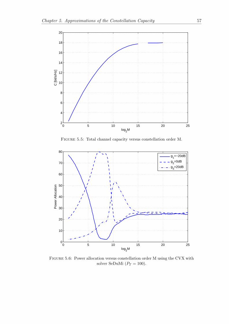
Chapter 5. Approximations of the Constellation Capacity 57
0 5 10 15 20 252
4
6
8
10
12
14
16
18
20
log2M
C [b
it/s/
Hz]
Figure 5.5: Total channel capacity versus constellation order M.
0 5 10 15 20 250
10
20
30
40
50
60
70
80
log2M
Pow
er A
lloca
tion
g
1=−20dB
g2=0dB
g3=20dB
Figure 5.6: Power allocation versus constellation order M using the CVX withsolver SeDuMi (PT = 100).
Chapter 5. Approximations of the Constellation Capacity 58
At first, the CVX was used to compute the OPA using (5.22) and (5.23), which
is a convex optimization problem. However, abnormal behaviors are found in the
results, and cvx status is ”failed” for certain points.
As shown in Figure 5.3, 5.4 and 5.5, there are gaps on the curves which correspond
to points where cvx status is ”failed”. The gaps still exist even though the pre-
cision is set to be low. The other solver SeDuMi is used instead for comparison,
and the OPA is calculated which is shown in Figure 5.6.
As shown in Figure 5.6, the total power constraint cannot be satisfied for higher
order constellations after SeDuMi is used. For SeDuMi, cvx status are ”solved”
everywhere and there is no gap on the curves. However, the fluctuation at low con-
stellation cardinality and incorrect saturation at higher constellation cardinality
makes it unacceptable.
Alternatives based on the bisection method was used, instead of the CVX. The
power allocation (5.24) is a monotonic function of λ, where pk decreases with λ,
and the other terms Mk and gk are all known constants. Therefore the bisection
method is utilized to compute λ from the total power constraint. The OPA for the
regular WF based on (5.26) and (5.27) is shown in the same graph for comparison.
As shown in Figure 5.7, 5.8 and 5.9, the gaps in Figure 5.3, 5.4 and 5.5 are filled.
Moreover, the curves do not fluctuate abnormally as Figure 5.6.
As shown in Figure 5.7, the AOPA is identical to the regular WF OPA when
the constellation order M is sufficiently large. However, it is the opposite of the
regular WF when M is less than 25, where the worst channel gets the most power,
and the best channel gets the least power.
As shown in Figure 5.8, the constellation capacity approaches the WF capacity
when the constellation order M is sufficiently large. The sub-channels with higher
gains have higher constellation-constrained capacity.
As shown in Figure 5.9, the constellation capacity increases with the constellation
order M . It converges to the channel capacity when M is sufficiently large. It
also validates (5.2) in that the constellation capacity can never exceed the channel
capacity.
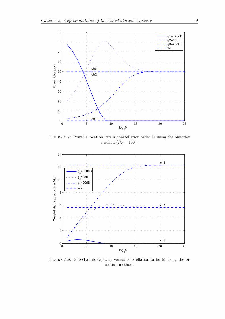
Chapter 5. Approximations of the Constellation Capacity 59
0 5 10 15 20 250
10
20
30
40
50
60
70
80
90
log2M
Pow
er A
lloca
tion
ch3
ch2
ch1
g1=−20dBg2=0dBg3=20dBWF
Figure 5.7: Power allocation versus constellation order M using the bisectionmethod (PT = 100).
0 5 10 15 20 250
2
4
6
8
10
12
14
log2M
Con
stel
latio
n ca
paci
ty [b
it/s/
Hz]
ch3
ch2
ch1
g1=−20dB
g2=0dB
g3=20dB
WF
Figure 5.8: Sub-channel capacity versus constellation order M using the bi-section method.
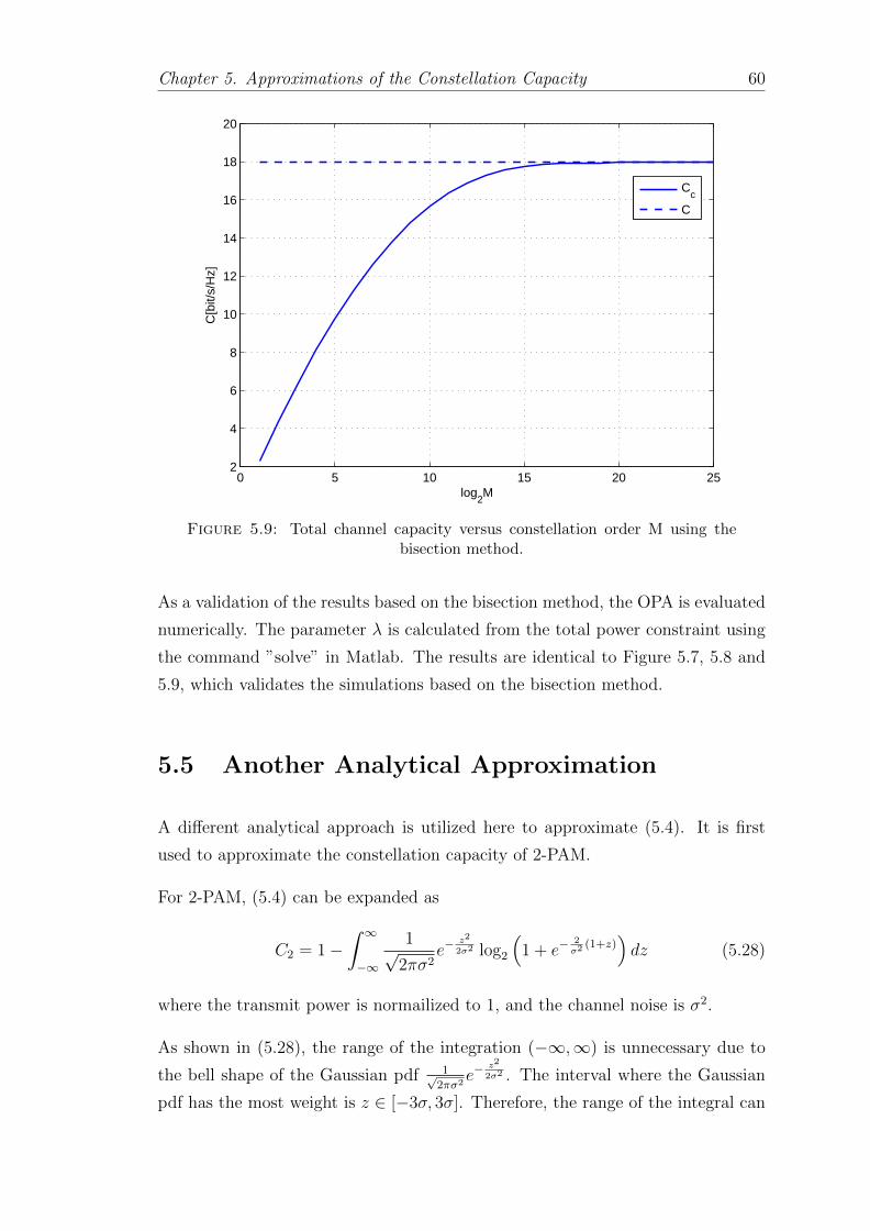
Chapter 5. Approximations of the Constellation Capacity 60
0 5 10 15 20 252
4
6
8
10
12
14
16
18
20
log2M
C[b
it/s/
Hz]
Cc
C
Figure 5.9: Total channel capacity versus constellation order M using thebisection method.
As a validation of the results based on the bisection method, the OPA is evaluated
numerically. The parameter λ is calculated from the total power constraint using
the command ”solve” in Matlab. The results are identical to Figure 5.7, 5.8 and
5.9, which validates the simulations based on the bisection method.
5.5 Another Analytical Approximation
A different analytical approach is utilized here to approximate (5.4). It is first
used to approximate the constellation capacity of 2-PAM.
For 2-PAM, (5.4) can be expanded as
C2 = 1−∫ ∞−∞
1√2πσ2
e−z2
2σ2 log2
(1 + e−
2σ2
(1+z))dz (5.28)
where the transmit power is normailized to 1, and the channel noise is σ2.
As shown in (5.28), the range of the integration (−∞,∞) is unnecessary due to
the bell shape of the Gaussian pdf 1√2πσ2
e−z2
2σ2 . The interval where the Gaussian
pdf has the most weight is z ∈ [−3σ, 3σ]. Therefore, the range of the integral can
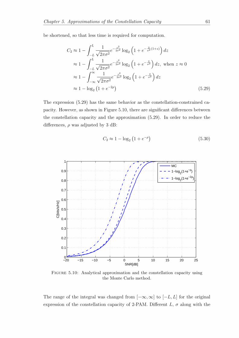
Chapter 5. Approximations of the Constellation Capacity 61
be shortened, so that less time is required for computation.
C2 ≈ 1−∫ L
−L
1√2πσ2
e−z2
2σ2 log2
(1 + e−
2σ2
(1+z))dz
≈ 1−∫ L
−L
1√2πσ2
e−z2
2σ2 log2
(1 + e−
2σ2
)dz, when z ≈ 0
≈ 1−∫ ∞−∞
1√2πσ2
e−z2
2σ2 log2
(1 + e−
2σ2
)dz
≈ 1− log2
(1 + e−2ρ
)(5.29)
The expression (5.29) has the same behavior as the constellation-constrained ca-
pacity. However, as shown in Figure 5.10, there are significant differences between
the constellation capacity and the approximation (5.29). In order to reduce the
differences, ρ was adjusted by 3 dB:
C2 ≈ 1− log2
(1 + e−ρ
)(5.30)
−20 −15 −10 −5 0 5 10 15 20 250
0.1
0.2
0.3
0.4
0.5
0.6
0.7
0.8
0.9
1
SNR[dB]
C[b
its/s
/Hz]
MC
1−log2(1+e−ρ)
1−log2(1+e−2ρ)
Figure 5.10: Analytical approximation and the constellation capacity usingthe Monte Carlo method.
The range of the integral was changed from [−∞,∞] to [−L,L] for the original
expression of the constellation capacity of 2-PAM. Different L, σ along with the
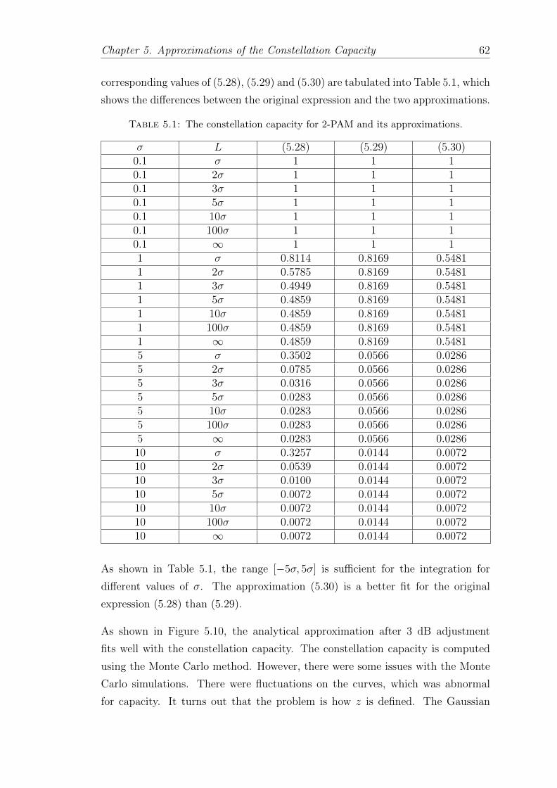
Chapter 5. Approximations of the Constellation Capacity 62
corresponding values of (5.28), (5.29) and (5.30) are tabulated into Table 5.1, which
shows the differences between the original expression and the two approximations.
Table 5.1: The constellation capacity for 2-PAM and its approximations.
σ L (5.28) (5.29) (5.30)0.1 σ 1 1 10.1 2σ 1 1 10.1 3σ 1 1 10.1 5σ 1 1 10.1 10σ 1 1 10.1 100σ 1 1 10.1 ∞ 1 1 11 σ 0.8114 0.8169 0.54811 2σ 0.5785 0.8169 0.54811 3σ 0.4949 0.8169 0.54811 5σ 0.4859 0.8169 0.54811 10σ 0.4859 0.8169 0.54811 100σ 0.4859 0.8169 0.54811 ∞ 0.4859 0.8169 0.54815 σ 0.3502 0.0566 0.02865 2σ 0.0785 0.0566 0.02865 3σ 0.0316 0.0566 0.02865 5σ 0.0283 0.0566 0.02865 10σ 0.0283 0.0566 0.02865 100σ 0.0283 0.0566 0.02865 ∞ 0.0283 0.0566 0.028610 σ 0.3257 0.0144 0.007210 2σ 0.0539 0.0144 0.007210 3σ 0.0100 0.0144 0.007210 5σ 0.0072 0.0144 0.007210 10σ 0.0072 0.0144 0.007210 100σ 0.0072 0.0144 0.007210 ∞ 0.0072 0.0144 0.0072
As shown in Table 5.1, the range [−5σ, 5σ] is sufficient for the integration for
different values of σ. The approximation (5.30) is a better fit for the original
expression (5.28) than (5.29).
As shown in Figure 5.10, the analytical approximation after 3 dB adjustment
fits well with the constellation capacity. The constellation capacity is computed
using the Monte Carlo method. However, there were some issues with the Monte
Carlo simulations. There were fluctuations on the curves, which was abnormal
for capacity. It turns out that the problem is how z is defined. The Gaussian
Chapter 5. Approximations of the Constellation Capacity 63
random variable is z ∼ N(0, σ2) where σ2 changes with SNR. At first, a new z
was redefined with a new SNR at the beginning of every iteration, which caused
the abnormal fluctuations. In order to eliminate the fluctuations, a new Gaussian
random variable z1 is defined as z1 ∼ N(0, 1) before interations start. Therefore
the Gaussian random variable z for every SNR is z = σz1, which provides smooth
results.
An approximation for 4-QAM can also be obtained from (5.29), since 4-QAM
is a composition of two 2-PAM in quadrature, each with half the power. The
constellation capacity for 4-QAM can be approximated as:
C4 ≈ 2(1− log2(1 + e−ρ)
)(5.31)
For higher order constellations, (5.4) can be written as:
CM = log2M −∑j
1
M
∫ ∞−∞
1√2πσ2
e−z2
2σ2 log2
1 +∑i 6=j
e
(−d2ij2σ2−zdij
σ2
) dz (5.32)
where dii = djj = 0.
In the high SNR region where σ → 0, the constellation capacity (5.32) can be
approximated as:
CM ≈ log2M −∑j
1
Mlog2
(1 +
∑i 6=j
e−d2ij2σ2
)(5.33)
which can be manipulated in a similar way to (5.29). Some of the terms in the
internal summation are negligible due to the high SNR. Therefore (5.33) can be
further simplified as:
CM ≈ log2M −∑j
1
Mlog2
(1 +
∑i 6=j
e−d2ij
2ρ
)(5.34)
≈ log2M −1
M·M log2
(1 + e
−d2min2
ρ
)(5.35)
= log2M − log2
(1 + e−
d2min2
ρ
)(5.36)
where ρ� 1.
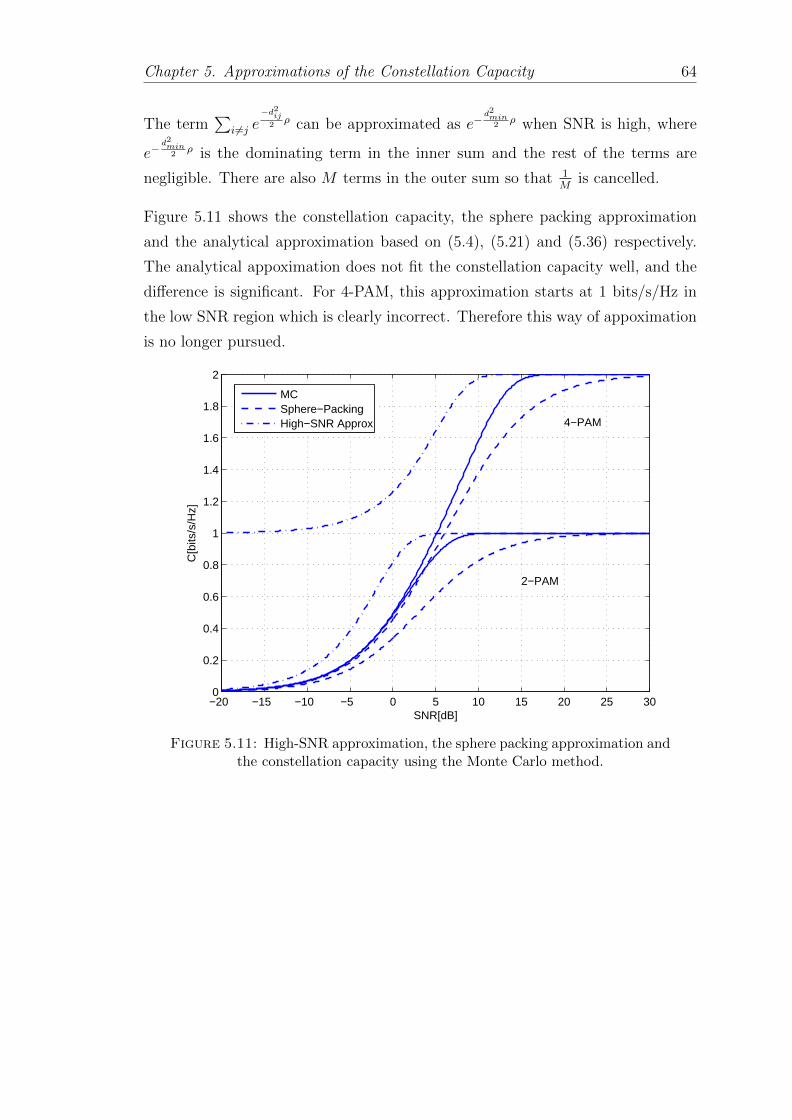
Chapter 5. Approximations of the Constellation Capacity 64
The term∑
i 6=j e−d2ij
2ρ can be approximated as e−
d2min2
ρ when SNR is high, where
e−d2min
2ρ is the dominating term in the inner sum and the rest of the terms are
negligible. There are also M terms in the outer sum so that 1M
is cancelled.
Figure 5.11 shows the constellation capacity, the sphere packing approximation
and the analytical approximation based on (5.4), (5.21) and (5.36) respectively.
The analytical appoximation does not fit the constellation capacity well, and the
difference is significant. For 4-PAM, this approximation starts at 1 bits/s/Hz in
the low SNR region which is clearly incorrect. Therefore this way of appoximation
is no longer pursued.
−20 −15 −10 −5 0 5 10 15 20 25 300
0.2
0.4
0.6
0.8
1
1.2
1.4
1.6
1.8
2
SNR[dB]
C[b
its/s
/Hz]
2−PAM
4−PAM
MCSphere−PackingHigh−SNR Approx
Figure 5.11: High-SNR approximation, the sphere packing approximation andthe constellation capacity using the Monte Carlo method.
Chapter 5. Approximations of the Constellation Capacity 65
5.6 Summary
The constellation capacity is discussed in this chapter, for which an explicit ex-
pression can be found in [13]. It is a complicated expression containing an integral,
which makes it difficult to evaluate numerically. The Monte Carlo method is in-
troduced in this chapter in order to calculate the integral. Using the Monte Carlo
method, the integral turns into the computation of the mean of a Gaussian ran-
dom variable. It is unnecessary to integrate from −∞ to ∞, therefore, the range
of the integration can be shortened while the result remains reasonably accurate.
An approximation of the constellation capacity is derived based on the sphere
packing approach in this chapter. It is compared with the Gaussian channel ca-
pacity and the constellation-constrained capacity in [13]. The approximation is
close to the constellation-constrained capacity, whose key characteristics are also
preserved (i.e. concavity). Convex optimization can be used to obtain the OPA
of the sphere packing approximation, which turns into the regular WF when con-
stellation cardinality approaches ∞.
Many problems occur in the process of calculating the OPA for the sphere packing
approximation. The CVX was used to obtain the OPA at first, but the result was
not promising. A different solver was used instead of the default one. It takes
less time to process but the result fluctuates abnormally. In the end, the bisection
method was used instead, and it gave satisfying results.
Another analytical approximation of the constellation capacity is proposed. How-
ever, it only applies to 2-PAM after some manipulations and needs even more
adjustments for higher order constellations. There is no generalized expression for
arbitrary input distributions, therefore this direction is no longer pursued.
Chapter 6
Performance Analysis of the
MWF and its Approximations
6.1 Two Parallel Channels
Following the previous chapters, the difference in performance between the mer-
cury/waterfilling (MWF) and the constellation-constrained waterfilling (WF) is
now considered in-depth. Figure 4.5 shows the optimal power allocation (OPA)
of the MWF, while Figure 5.7 shows the approximated OPA of the constellation-
constrained WF (AOPA). To explore the difference in performance between the
two power allocation (PA) schemes, the same set of notations is used and several
expressions are modified. After some modification, the constellation-constrained
WF can be expressed as,
pk =1
2gkP
(√(Mk − 1)2 +
4gkλ
(Mk − 1)− (Mk + 1)
), gk > λ
(1− 1
Mk
)−1(6.1)
pk = 0, gk ≤ λ
(1− 1
Mk
)−1(6.2)
where P is the average power constraint in (3.2), pk is the normalized power, and
the actual power on each sub-channel is pkP . The constellation cardinality is set
to the same value for each sub-channel, i.e., Mk = M .
66
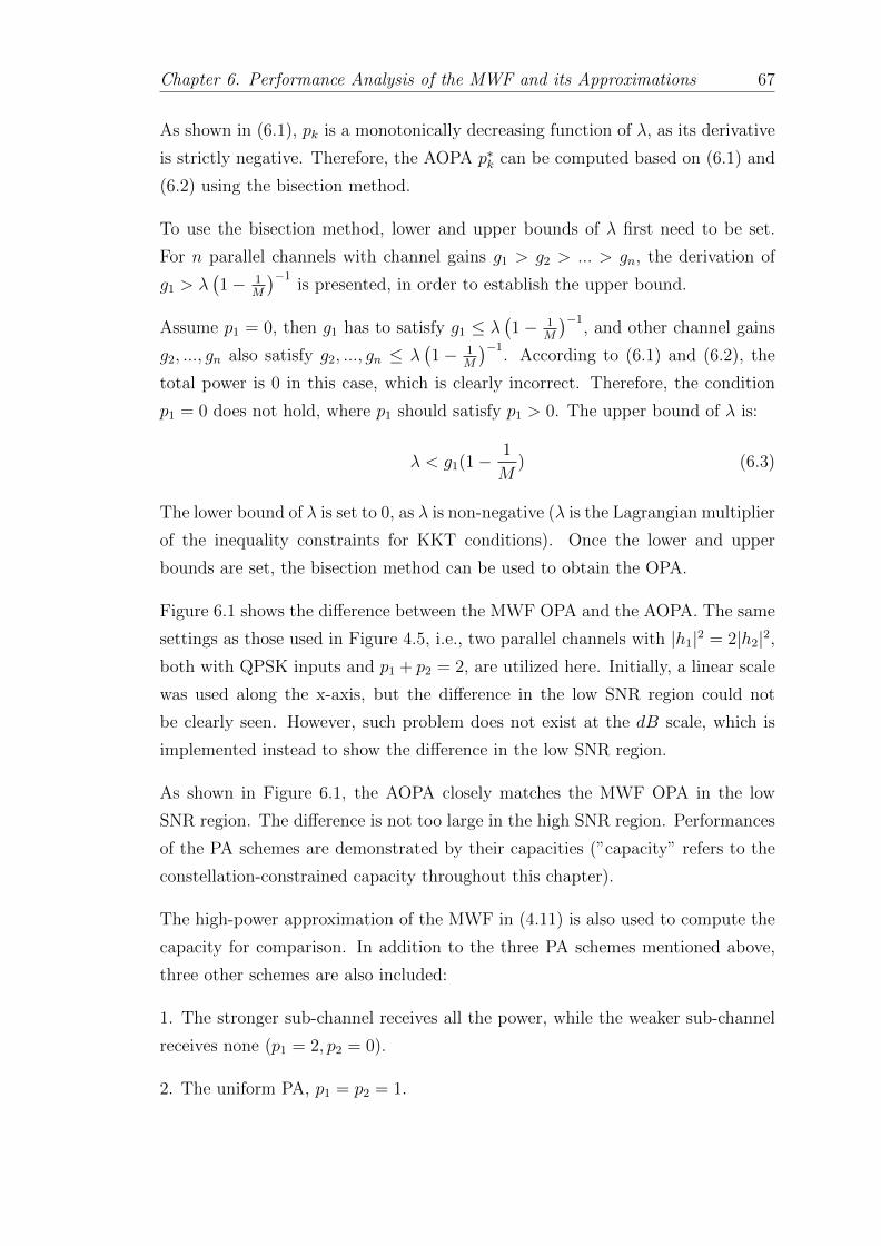
Chapter 6. Performance Analysis of the MWF and its Approximations 67
As shown in (6.1), pk is a monotonically decreasing function of λ, as its derivative
is strictly negative. Therefore, the AOPA p∗k can be computed based on (6.1) and
(6.2) using the bisection method.
To use the bisection method, lower and upper bounds of λ first need to be set.
For n parallel channels with channel gains g1 > g2 > ... > gn, the derivation of
g1 > λ(1− 1
M
)−1is presented, in order to establish the upper bound.
Assume p1 = 0, then g1 has to satisfy g1 ≤ λ(1− 1
M
)−1, and other channel gains
g2, ..., gn also satisfy g2, ..., gn ≤ λ(1− 1
M
)−1. According to (6.1) and (6.2), the
total power is 0 in this case, which is clearly incorrect. Therefore, the condition
p1 = 0 does not hold, where p1 should satisfy p1 > 0. The upper bound of λ is:
λ < g1(1−1
M) (6.3)
The lower bound of λ is set to 0, as λ is non-negative (λ is the Lagrangian multiplier
of the inequality constraints for KKT conditions). Once the lower and upper
bounds are set, the bisection method can be used to obtain the OPA.
Figure 6.1 shows the difference between the MWF OPA and the AOPA. The same
settings as those used in Figure 4.5, i.e., two parallel channels with |h1|2 = 2|h2|2,both with QPSK inputs and p1 + p2 = 2, are utilized here. Initially, a linear scale
was used along the x-axis, but the difference in the low SNR region could not
be clearly seen. However, such problem does not exist at the dB scale, which is
implemented instead to show the difference in the low SNR region.
As shown in Figure 6.1, the AOPA closely matches the MWF OPA in the low
SNR region. The difference is not too large in the high SNR region. Performances
of the PA schemes are demonstrated by their capacities (”capacity” refers to the
constellation-constrained capacity throughout this chapter).
The high-power approximation of the MWF in (4.11) is also used to compute the
capacity for comparison. In addition to the three PA schemes mentioned above,
three other schemes are also included:
1. The stronger sub-channel receives all the power, while the weaker sub-channel
receives none (p1 = 2, p2 = 0).
2. The uniform PA, p1 = p2 = 1.
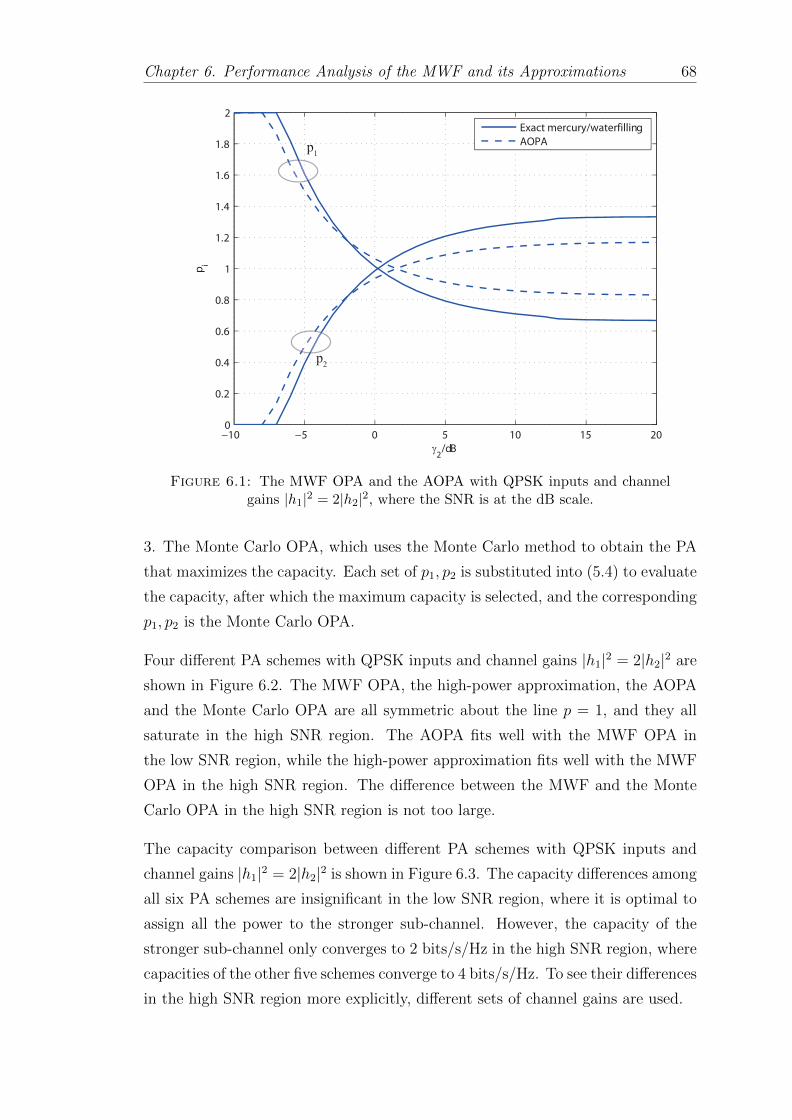
Chapter 6. Performance Analysis of the MWF and its Approximations 68
−10 −5 0 5 10 15 200
0.2
0.4
0.6
0.8
1
1.2
1.4
1.6
1.8
2
γ2
/dB
pi
Exact mercury/waterfilling
AOPAp1
p2
Figure 6.1: The MWF OPA and the AOPA with QPSK inputs and channelgains |h1|2 = 2|h2|2, where the SNR is at the dB scale.
3. The Monte Carlo OPA, which uses the Monte Carlo method to obtain the PA
that maximizes the capacity. Each set of p1, p2 is substituted into (5.4) to evaluate
the capacity, after which the maximum capacity is selected, and the corresponding
p1, p2 is the Monte Carlo OPA.
Four different PA schemes with QPSK inputs and channel gains |h1|2 = 2|h2|2 are
shown in Figure 6.2. The MWF OPA, the high-power approximation, the AOPA
and the Monte Carlo OPA are all symmetric about the line p = 1, and they all
saturate in the high SNR region. The AOPA fits well with the MWF OPA in
the low SNR region, while the high-power approximation fits well with the MWF
OPA in the high SNR region. The difference between the MWF and the Monte
Carlo OPA in the high SNR region is not too large.
The capacity comparison between different PA schemes with QPSK inputs and
channel gains |h1|2 = 2|h2|2 is shown in Figure 6.3. The capacity differences among
all six PA schemes are insignificant in the low SNR region, where it is optimal to
assign all the power to the stronger sub-channel. However, the capacity of the
stronger sub-channel only converges to 2 bits/s/Hz in the high SNR region, where
capacities of the other five schemes converge to 4 bits/s/Hz. To see their differences
in the high SNR region more explicitly, different sets of channel gains are used.
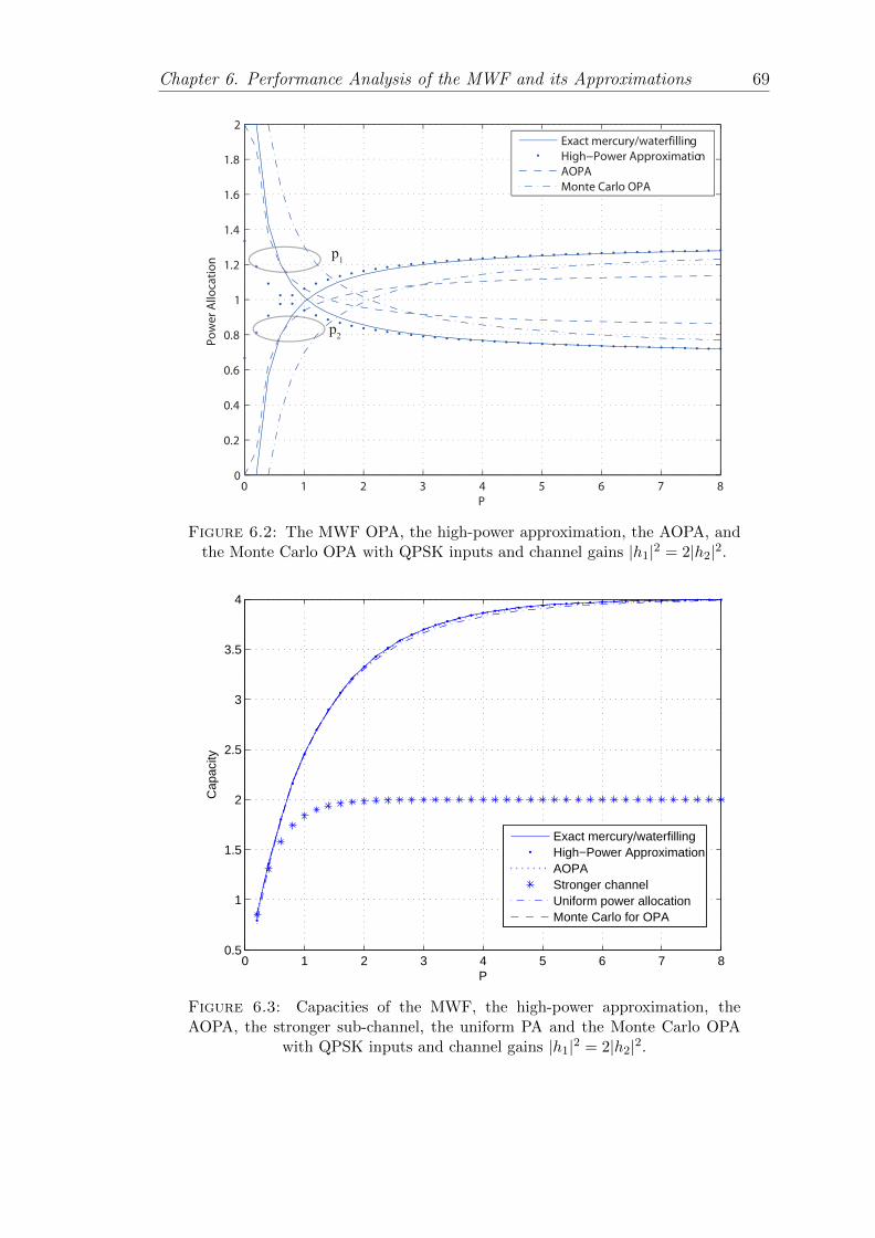
Chapter 6. Performance Analysis of the MWF and its Approximations 69
0 1 2 3 4 5 6 7 80
0.2
0.4
0.6
0.8
1
1.2
1.4
1.6
1.8
2
P
Po
we
r A
lloca
tio
n
Exact mercury/waterfilling
High−Power Approximation
AOPA
Monte Carlo OPA
p1
p2
Figure 6.2: The MWF OPA, the high-power approximation, the AOPA, andthe Monte Carlo OPA with QPSK inputs and channel gains |h1|2 = 2|h2|2.
0 1 2 3 4 5 6 7 80.5
1
1.5
2
2.5
3
3.5
4
P
Cap
acity
Exact mercury/waterfillingHigh−Power ApproximationAOPAStronger channelUniform power allocationMonte Carlo for OPA
Figure 6.3: Capacities of the MWF, the high-power approximation, theAOPA, the stronger sub-channel, the uniform PA and the Monte Carlo OPA
with QPSK inputs and channel gains |h1|2 = 2|h2|2.
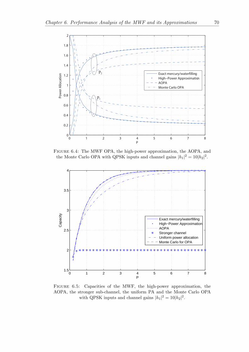
Chapter 6. Performance Analysis of the MWF and its Approximations 70
0 1 2 3 4 5 6 7 80
0.2
0.4
0.6
0.8
1
1.2
1.4
1.6
1.8
2
P
Po
we
r A
lloca
tio
n
Exact mercury/waterfilling
High−Power Approximation
AOPA
Monte Carlo OPA
p2
p1
Figure 6.4: The MWF OPA, the high-power approximation, the AOPA, andthe Monte Carlo OPA with QPSK inputs and channel gains |h1|2 = 10|h2|2.
0 1 2 3 4 5 6 7 81.5
2
2.5
3
3.5
4
P
Cap
acity
Exact mercury/waterfillingHigh−Power ApproximationAOPAStronger channelUniform power allocationMonte Carlo for OPA
Figure 6.5: Capacities of the MWF, the high-power approximation, theAOPA, the stronger sub-channel, the uniform PA and the Monte Carlo OPA
with QPSK inputs and channel gains |h1|2 = 10|h2|2.
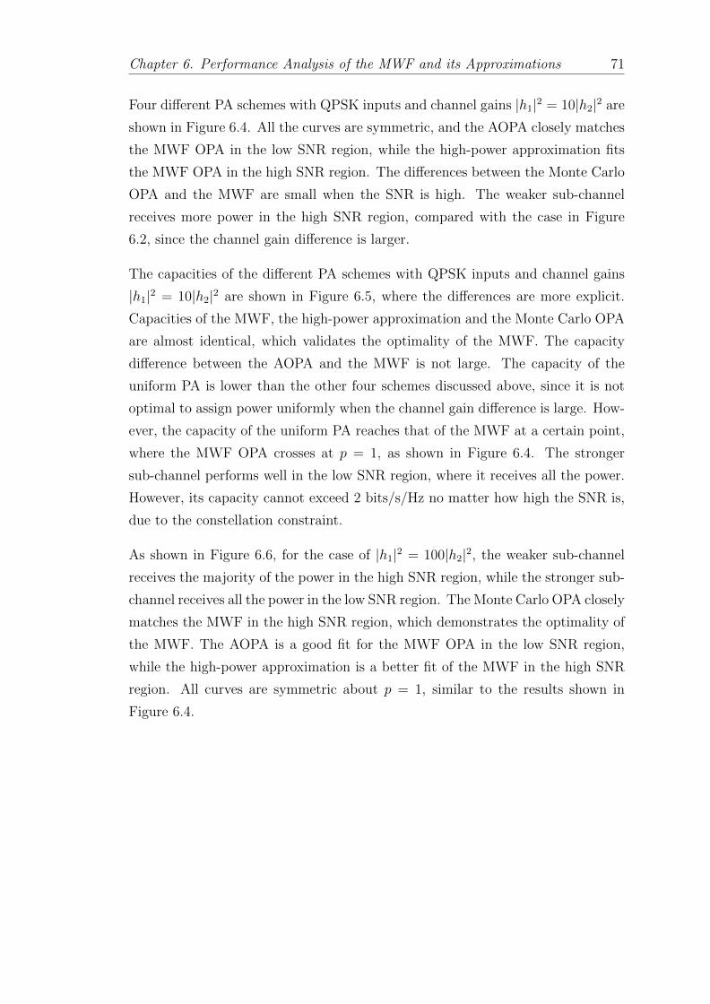
Chapter 6. Performance Analysis of the MWF and its Approximations 71
Four different PA schemes with QPSK inputs and channel gains |h1|2 = 10|h2|2 are
shown in Figure 6.4. All the curves are symmetric, and the AOPA closely matches
the MWF OPA in the low SNR region, while the high-power approximation fits
the MWF OPA in the high SNR region. The differences between the Monte Carlo
OPA and the MWF are small when the SNR is high. The weaker sub-channel
receives more power in the high SNR region, compared with the case in Figure
6.2, since the channel gain difference is larger.
The capacities of the different PA schemes with QPSK inputs and channel gains
|h1|2 = 10|h2|2 are shown in Figure 6.5, where the differences are more explicit.
Capacities of the MWF, the high-power approximation and the Monte Carlo OPA
are almost identical, which validates the optimality of the MWF. The capacity
difference between the AOPA and the MWF is not large. The capacity of the
uniform PA is lower than the other four schemes discussed above, since it is not
optimal to assign power uniformly when the channel gain difference is large. How-
ever, the capacity of the uniform PA reaches that of the MWF at a certain point,
where the MWF OPA crosses at p = 1, as shown in Figure 6.4. The stronger
sub-channel performs well in the low SNR region, where it receives all the power.
However, its capacity cannot exceed 2 bits/s/Hz no matter how high the SNR is,
due to the constellation constraint.
As shown in Figure 6.6, for the case of |h1|2 = 100|h2|2, the weaker sub-channel
receives the majority of the power in the high SNR region, while the stronger sub-
channel receives all the power in the low SNR region. The Monte Carlo OPA closely
matches the MWF in the high SNR region, which demonstrates the optimality of
the MWF. The AOPA is a good fit for the MWF OPA in the low SNR region,
while the high-power approximation is a better fit of the MWF in the high SNR
region. All curves are symmetric about p = 1, similar to the results shown in
Figure 6.4.
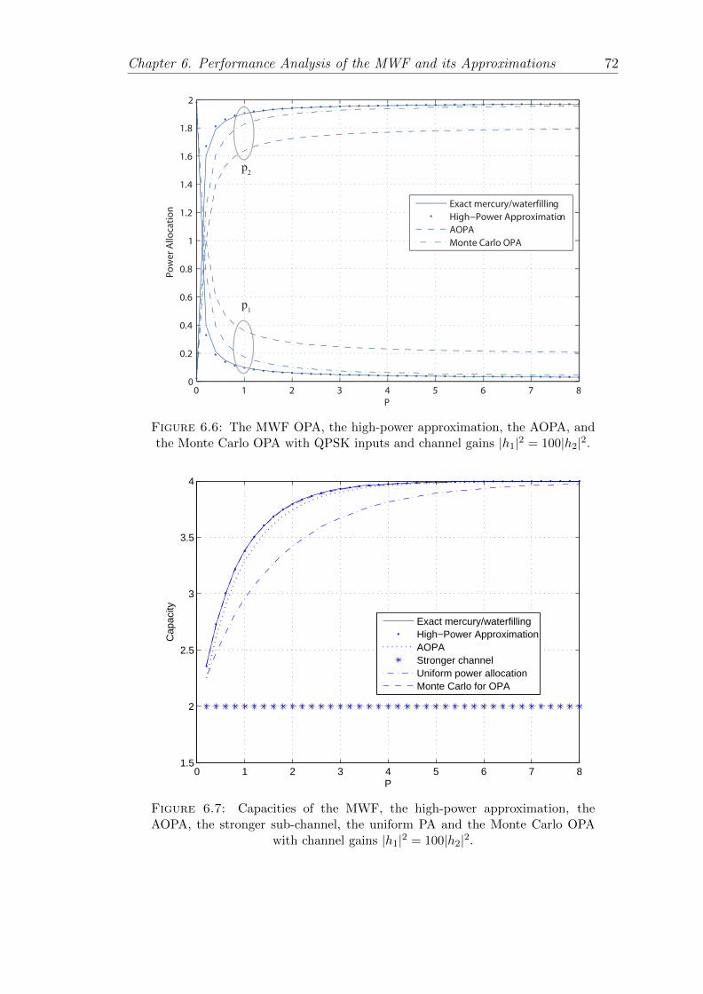
Chapter 6. Performance Analysis of the MWF and its Approximations 72
0 1 2 3 4 5 6 7 80
0.2
0.4
0.6
0.8
1
1.2
1.4
1.6
1.8
2
P
Po
we
r A
lloca
tio
n
Exact mercury/waterfilling
High−Power Approximation
AOPA
Monte Carlo OPA
p2
p1
Figure 6.6: The MWF OPA, the high-power approximation, the AOPA, andthe Monte Carlo OPA with QPSK inputs and channel gains |h1|2 = 100|h2|2.
0 1 2 3 4 5 6 7 81.5
2
2.5
3
3.5
4
P
Cap
acity
Exact mercury/waterfillingHigh−Power ApproximationAOPAStronger channelUniform power allocationMonte Carlo for OPA
Figure 6.7: Capacities of the MWF, the high-power approximation, theAOPA, the stronger sub-channel, the uniform PA and the Monte Carlo OPA
with channel gains |h1|2 = 100|h2|2.
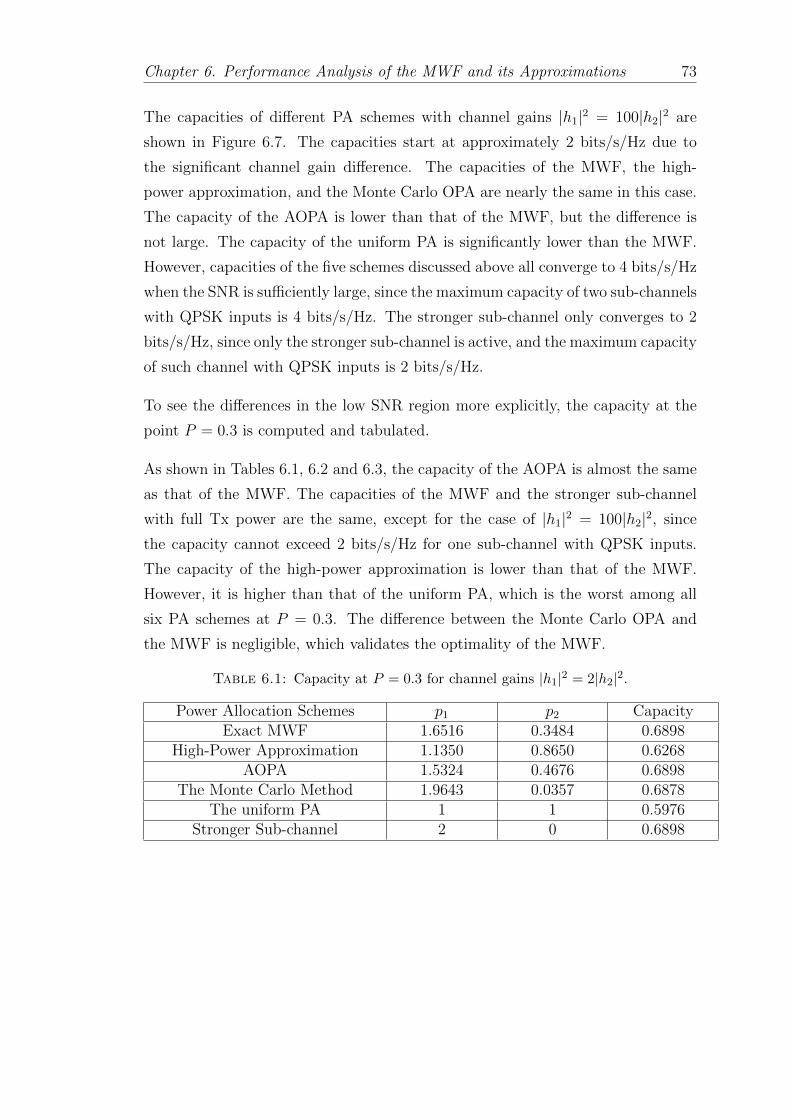
Chapter 6. Performance Analysis of the MWF and its Approximations 73
The capacities of different PA schemes with channel gains |h1|2 = 100|h2|2 are
shown in Figure 6.7. The capacities start at approximately 2 bits/s/Hz due to
the significant channel gain difference. The capacities of the MWF, the high-
power approximation, and the Monte Carlo OPA are nearly the same in this case.
The capacity of the AOPA is lower than that of the MWF, but the difference is
not large. The capacity of the uniform PA is significantly lower than the MWF.
However, capacities of the five schemes discussed above all converge to 4 bits/s/Hz
when the SNR is sufficiently large, since the maximum capacity of two sub-channels
with QPSK inputs is 4 bits/s/Hz. The stronger sub-channel only converges to 2
bits/s/Hz, since only the stronger sub-channel is active, and the maximum capacity
of such channel with QPSK inputs is 2 bits/s/Hz.
To see the differences in the low SNR region more explicitly, the capacity at the
point P = 0.3 is computed and tabulated.
As shown in Tables 6.1, 6.2 and 6.3, the capacity of the AOPA is almost the same
as that of the MWF. The capacities of the MWF and the stronger sub-channel
with full Tx power are the same, except for the case of |h1|2 = 100|h2|2, since
the capacity cannot exceed 2 bits/s/Hz for one sub-channel with QPSK inputs.
The capacity of the high-power approximation is lower than that of the MWF.
However, it is higher than that of the uniform PA, which is the worst among all
six PA schemes at P = 0.3. The difference between the Monte Carlo OPA and
the MWF is negligible, which validates the optimality of the MWF.
Table 6.1: Capacity at P = 0.3 for channel gains |h1|2 = 2|h2|2.
Power Allocation Schemes p1 p2 CapacityExact MWF 1.6516 0.3484 0.6898
High-Power Approximation 1.1350 0.8650 0.6268AOPA 1.5324 0.4676 0.6898
The Monte Carlo Method 1.9643 0.0357 0.6878The uniform PA 1 1 0.5976
Stronger Sub-channel 2 0 0.6898
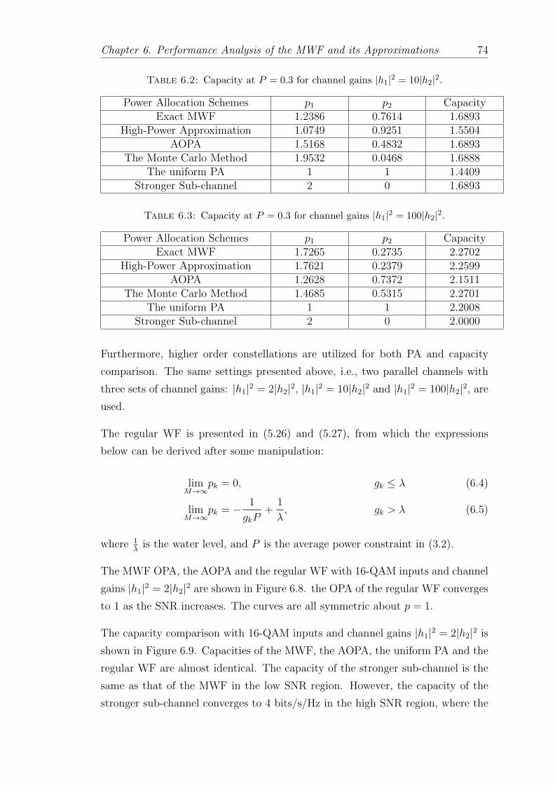
Chapter 6. Performance Analysis of the MWF and its Approximations 74
Table 6.2: Capacity at P = 0.3 for channel gains |h1|2 = 10|h2|2.
Power Allocation Schemes p1 p2 CapacityExact MWF 1.2386 0.7614 1.6893
High-Power Approximation 1.0749 0.9251 1.5504AOPA 1.5168 0.4832 1.6893
The Monte Carlo Method 1.9532 0.0468 1.6888The uniform PA 1 1 1.4409
Stronger Sub-channel 2 0 1.6893
Table 6.3: Capacity at P = 0.3 for channel gains |h1|2 = 100|h2|2.
Power Allocation Schemes p1 p2 CapacityExact MWF 1.7265 0.2735 2.2702
High-Power Approximation 1.7621 0.2379 2.2599AOPA 1.2628 0.7372 2.1511
The Monte Carlo Method 1.4685 0.5315 2.2701The uniform PA 1 1 2.2008
Stronger Sub-channel 2 0 2.0000
Furthermore, higher order constellations are utilized for both PA and capacity
comparison. The same settings presented above, i.e., two parallel channels with
three sets of channel gains: |h1|2 = 2|h2|2, |h1|2 = 10|h2|2 and |h1|2 = 100|h2|2, are
used.
The regular WF is presented in (5.26) and (5.27), from which the expressions
below can be derived after some manipulation:
limM→∞
pk = 0, gk ≤ λ (6.4)
limM→∞
pk = − 1
gkP+
1
λ, gk > λ (6.5)
where 1λ
is the water level, and P is the average power constraint in (3.2).
The MWF OPA, the AOPA and the regular WF with 16-QAM inputs and channel
gains |h1|2 = 2|h2|2 are shown in Figure 6.8. the OPA of the regular WF converges
to 1 as the SNR increases. The curves are all symmetric about p = 1.
The capacity comparison with 16-QAM inputs and channel gains |h1|2 = 2|h2|2 is
shown in Figure 6.9. Capacities of the MWF, the AOPA, the uniform PA and the
regular WF are almost identical. The capacity of the stronger sub-channel is the
same as that of the MWF in the low SNR region. However, the capacity of the
stronger sub-channel converges to 4 bits/s/Hz in the high SNR region, where the
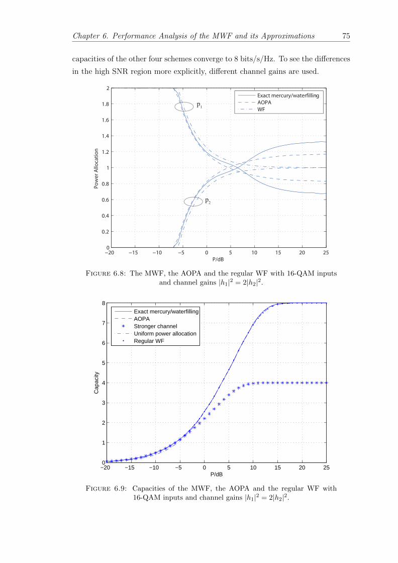
Chapter 6. Performance Analysis of the MWF and its Approximations 75
capacities of the other four schemes converge to 8 bits/s/Hz. To see the differences
in the high SNR region more explicitly, different channel gains are used.
−20 −15 −10 −5 0 5 10 15 20 250
0.2
0.4
0.6
0.8
1
1.2
1.4
1.6
1.8
2
P/dB
Po
we
r A
lloca
tio
n
Exact mercury/waterfilling
AOPA
WFp1
p2
Figure 6.8: The MWF, the AOPA and the regular WF with 16-QAM inputsand channel gains |h1|2 = 2|h2|2.
−20 −15 −10 −5 0 5 10 15 20 250
1
2
3
4
5
6
7
8
P/dB
Cap
acity
Exact mercury/waterfillingAOPAStronger channelUniform power allocationRegular WF
Figure 6.9: Capacities of the MWF, the AOPA and the regular WF with16-QAM inputs and channel gains |h1|2 = 2|h2|2.
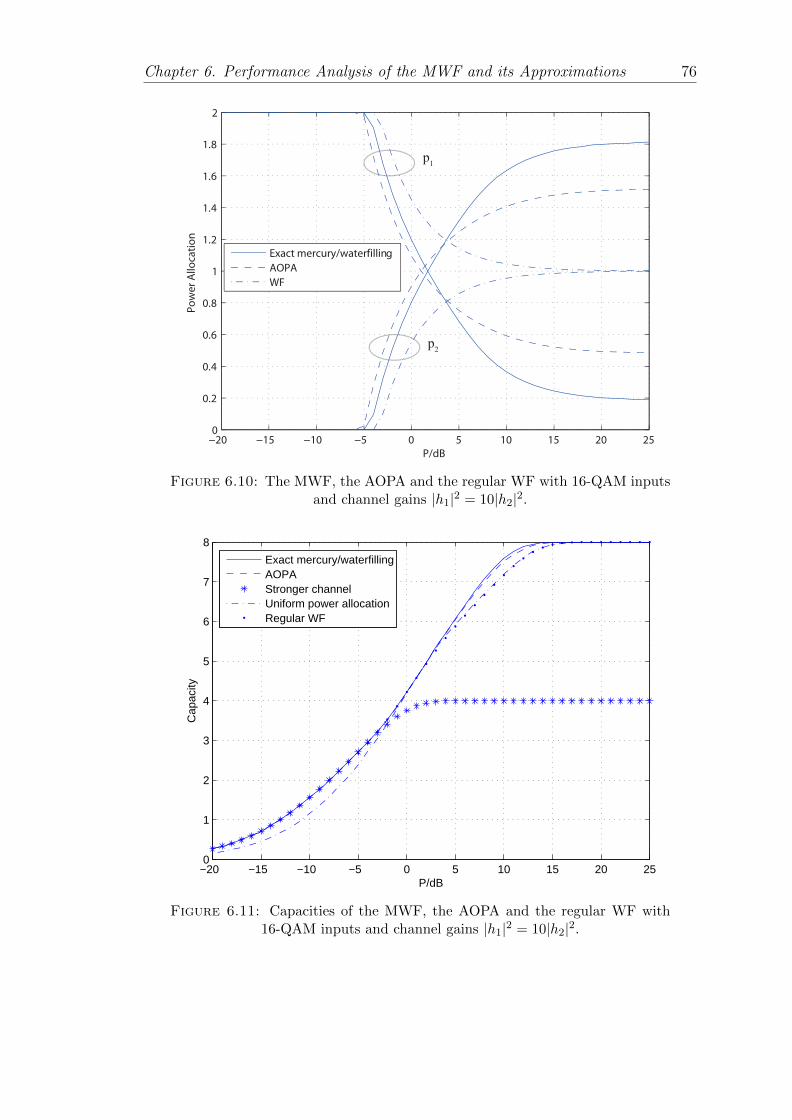
Chapter 6. Performance Analysis of the MWF and its Approximations 76
−20 −15 −10 −5 0 5 10 15 20 250
0.2
0.4
0.6
0.8
1
1.2
1.4
1.6
1.8
2
P/dB
Po
we
r A
lloca
tio
n
Exact mercury/waterfilling
AOPA
WF
p1
p2
Figure 6.10: The MWF, the AOPA and the regular WF with 16-QAM inputsand channel gains |h1|2 = 10|h2|2.
−20 −15 −10 −5 0 5 10 15 20 250
1
2
3
4
5
6
7
8
P/dB
Cap
acity
Exact mercury/waterfillingAOPAStronger channelUniform power allocationRegular WF
Figure 6.11: Capacities of the MWF, the AOPA and the regular WF with16-QAM inputs and channel gains |h1|2 = 10|h2|2.
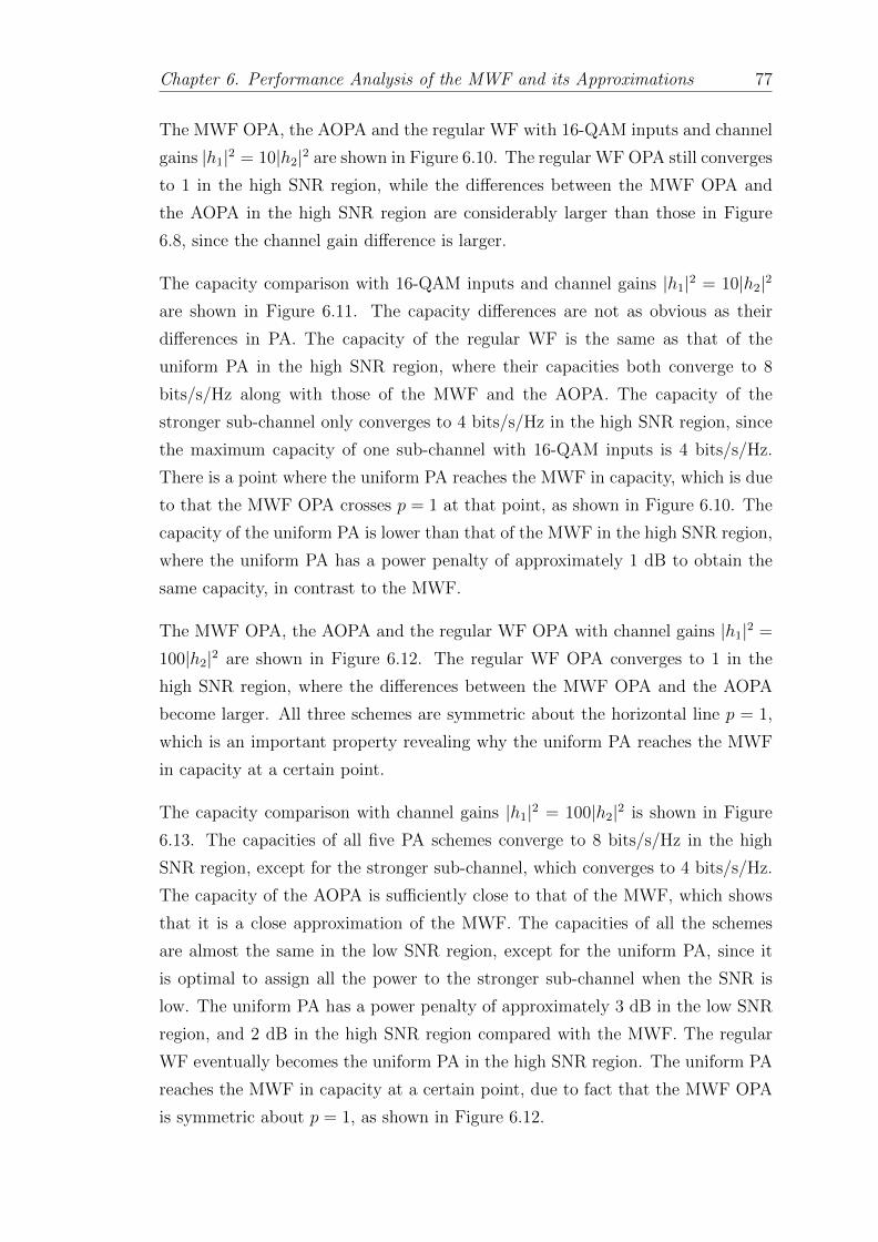
Chapter 6. Performance Analysis of the MWF and its Approximations 77
The MWF OPA, the AOPA and the regular WF with 16-QAM inputs and channel
gains |h1|2 = 10|h2|2 are shown in Figure 6.10. The regular WF OPA still converges
to 1 in the high SNR region, while the differences between the MWF OPA and
the AOPA in the high SNR region are considerably larger than those in Figure
6.8, since the channel gain difference is larger.
The capacity comparison with 16-QAM inputs and channel gains |h1|2 = 10|h2|2
are shown in Figure 6.11. The capacity differences are not as obvious as their
differences in PA. The capacity of the regular WF is the same as that of the
uniform PA in the high SNR region, where their capacities both converge to 8
bits/s/Hz along with those of the MWF and the AOPA. The capacity of the
stronger sub-channel only converges to 4 bits/s/Hz in the high SNR region, since
the maximum capacity of one sub-channel with 16-QAM inputs is 4 bits/s/Hz.
There is a point where the uniform PA reaches the MWF in capacity, which is due
to that the MWF OPA crosses p = 1 at that point, as shown in Figure 6.10. The
capacity of the uniform PA is lower than that of the MWF in the high SNR region,
where the uniform PA has a power penalty of approximately 1 dB to obtain the
same capacity, in contrast to the MWF.
The MWF OPA, the AOPA and the regular WF OPA with channel gains |h1|2 =
100|h2|2 are shown in Figure 6.12. The regular WF OPA converges to 1 in the
high SNR region, where the differences between the MWF OPA and the AOPA
become larger. All three schemes are symmetric about the horizontal line p = 1,
which is an important property revealing why the uniform PA reaches the MWF
in capacity at a certain point.
The capacity comparison with channel gains |h1|2 = 100|h2|2 is shown in Figure
6.13. The capacities of all five PA schemes converge to 8 bits/s/Hz in the high
SNR region, except for the stronger sub-channel, which converges to 4 bits/s/Hz.
The capacity of the AOPA is sufficiently close to that of the MWF, which shows
that it is a close approximation of the MWF. The capacities of all the schemes
are almost the same in the low SNR region, except for the uniform PA, since it
is optimal to assign all the power to the stronger sub-channel when the SNR is
low. The uniform PA has a power penalty of approximately 3 dB in the low SNR
region, and 2 dB in the high SNR region compared with the MWF. The regular
WF eventually becomes the uniform PA in the high SNR region. The uniform PA
reaches the MWF in capacity at a certain point, due to fact that the MWF OPA
is symmetric about p = 1, as shown in Figure 6.12.
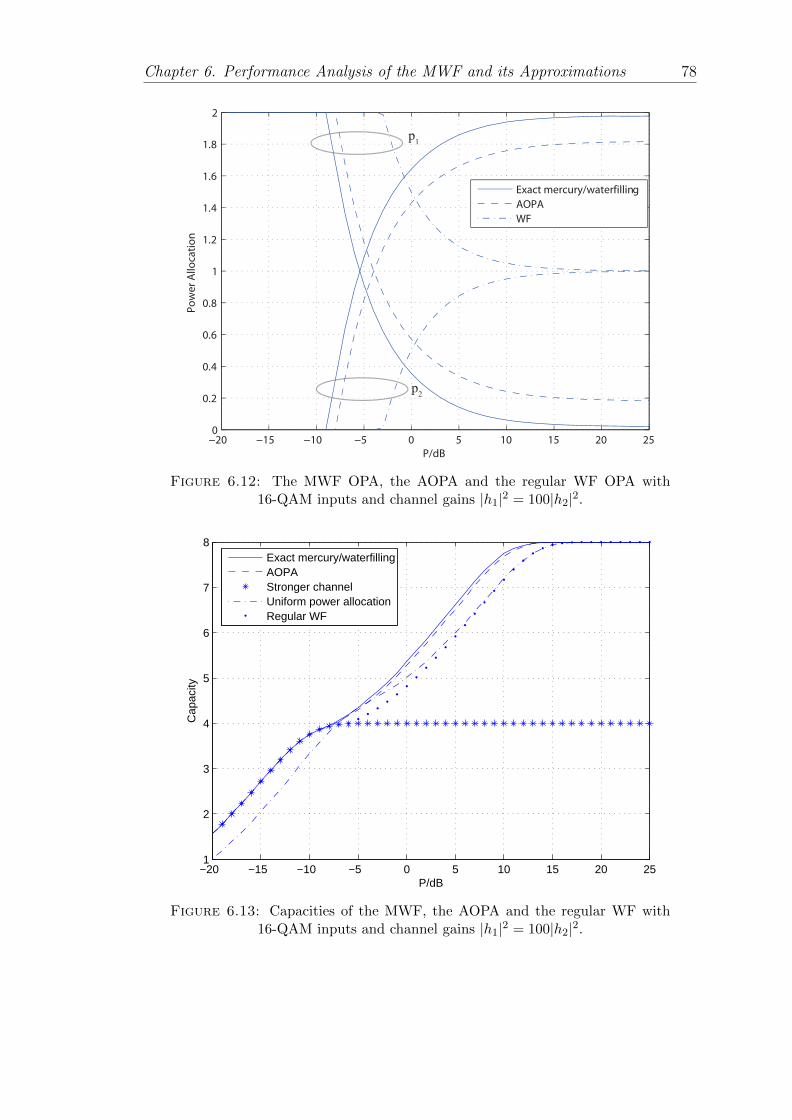
Chapter 6. Performance Analysis of the MWF and its Approximations 78
−20 −15 −10 −5 0 5 10 15 20 250
0.2
0.4
0.6
0.8
1
1.2
1.4
1.6
1.8
2
P/dB
Po
we
r A
lloca
tio
n
Exact mercury/waterfilling
AOPA
WF
p1
p2
Figure 6.12: The MWF OPA, the AOPA and the regular WF OPA with16-QAM inputs and channel gains |h1|2 = 100|h2|2.
−20 −15 −10 −5 0 5 10 15 20 251
2
3
4
5
6
7
8
P/dB
Cap
acity
Exact mercury/waterfillingAOPAStronger channelUniform power allocationRegular WF
Figure 6.13: Capacities of the MWF, the AOPA and the regular WF with16-QAM inputs and channel gains |h1|2 = 100|h2|2.
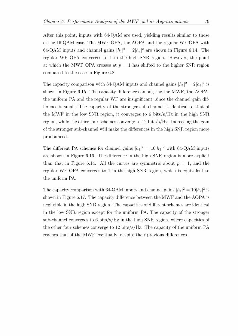
Chapter 6. Performance Analysis of the MWF and its Approximations 79
After this point, inputs with 64-QAM are used, yielding results similar to those
of the 16-QAM case. The MWF OPA, the AOPA and the regular WF OPA with
64-QAM inputs and channel gains |h1|2 = 2|h2|2 are shown in Figure 6.14. The
regular WF OPA converges to 1 in the high SNR region. However, the point
at which the MWF OPA crosses at p = 1 has shifted to the higher SNR region
compared to the case in Figure 6.8.
The capacity comparison with 64-QAM inputs and channel gains |h1|2 = 2|h2|2 is
shown in Figure 6.15. The capacity differences among the the MWF, the AOPA,
the uniform PA and the regular WF are insignificant, since the channel gain dif-
ference is small. The capacity of the stronger sub-channel is identical to that of
the MWF in the low SNR region, it converges to 6 bits/s/Hz in the high SNR
region, while the other four schemes converge to 12 bits/s/Hz. Increasing the gain
of the stronger sub-channel will make the differences in the high SNR region more
pronounced.
The different PA schemes for channel gains |h1|2 = 10|h2|2 with 64-QAM inputs
are shown in Figure 6.16. The difference in the high SNR region is more explicit
than that in Figure 6.14. All the curves are symmetric about p = 1, and the
regular WF OPA converges to 1 in the high SNR region, which is equivalent to
the uniform PA.
The capacity comparison with 64-QAM inputs and channel gains |h1|2 = 10|h2|2 is
shown in Figure 6.17. The capacity difference between the MWF and the AOPA is
negligible in the high SNR region. The capacities of different schemes are identical
in the low SNR region except for the uniform PA. The capacity of the stronger
sub-channel converges to 6 bits/s/Hz in the high SNR region, where capacities of
the other four schemes converge to 12 bits/s/Hz. The capacity of the uniform PA
reaches that of the MWF eventually, despite their previous differences.
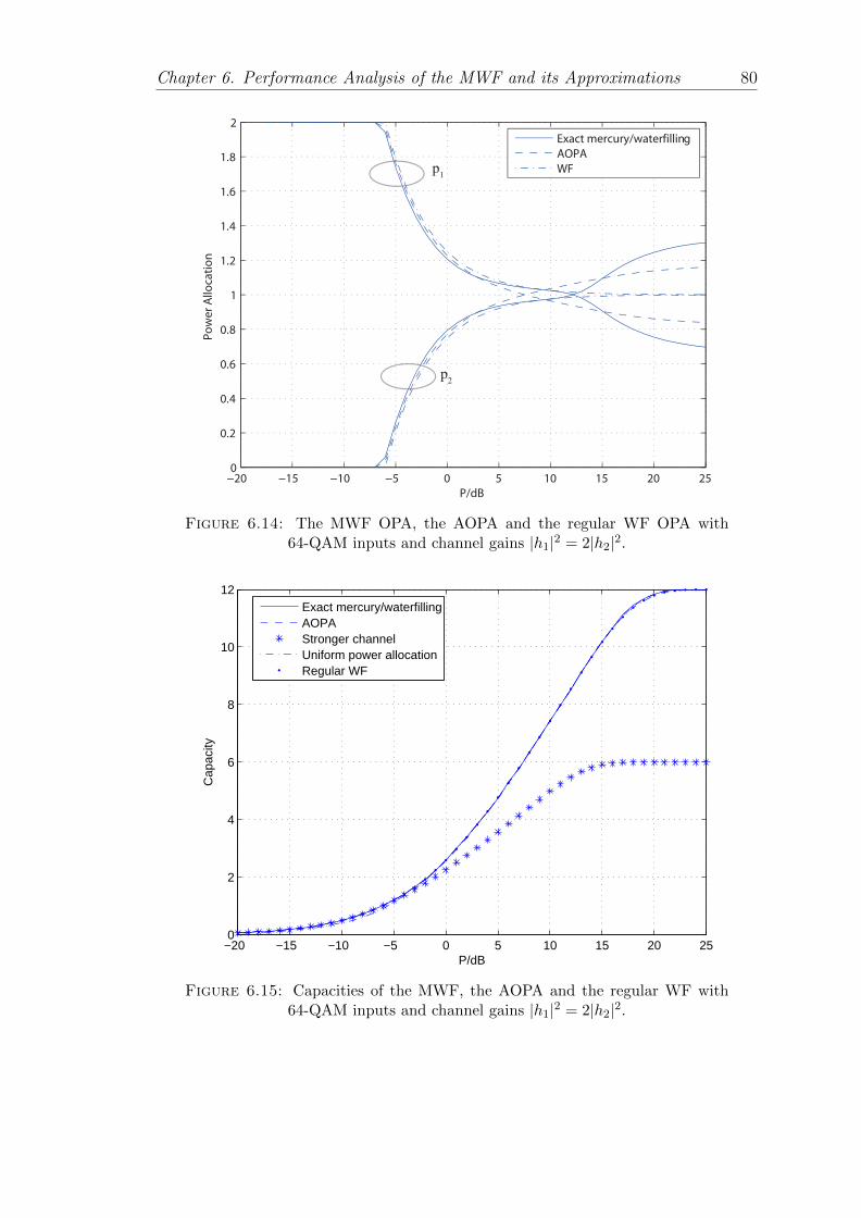
Chapter 6. Performance Analysis of the MWF and its Approximations 80
−20 −15 −10 −5 0 5 10 15 20 250
0.2
0.4
0.6
0.8
1
1.2
1.4
1.6
1.8
2
P/dB
Po
we
r A
lloca
tio
n
Exact mercury/waterfilling
AOPA
WFp1
p2
Figure 6.14: The MWF OPA, the AOPA and the regular WF OPA with64-QAM inputs and channel gains |h1|2 = 2|h2|2.
−20 −15 −10 −5 0 5 10 15 20 250
2
4
6
8
10
12
P/dB
Cap
acity
Exact mercury/waterfillingAOPAStronger channelUniform power allocationRegular WF
Figure 6.15: Capacities of the MWF, the AOPA and the regular WF with64-QAM inputs and channel gains |h1|2 = 2|h2|2.
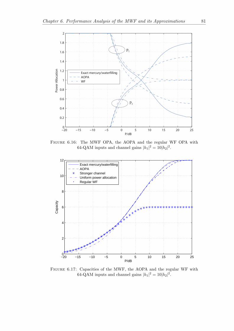
Chapter 6. Performance Analysis of the MWF and its Approximations 81
−20 −15 −10 −5 0 5 10 15 20 250
0.2
0.4
0.6
0.8
1
1.2
1.4
1.6
1.8
2
P/dB
Po
we
r A
lloca
tio
n
Exact mercury/waterfilling
AOPA
WF
p1
p2
Figure 6.16: The MWF OPA, the AOPA and the regular WF OPA with64-QAM inputs and channel gains |h1|2 = 10|h2|2.
−20 −15 −10 −5 0 5 10 15 20 250
2
4
6
8
10
12
P/dB
Cap
acity
Exact mercury/waterfillingAOPAStronger channelUniform power allocationRegular WF
Figure 6.17: Capacities of the MWF, the AOPA and the regular WF with64-QAM inputs and channel gains |h1|2 = 10|h2|2.
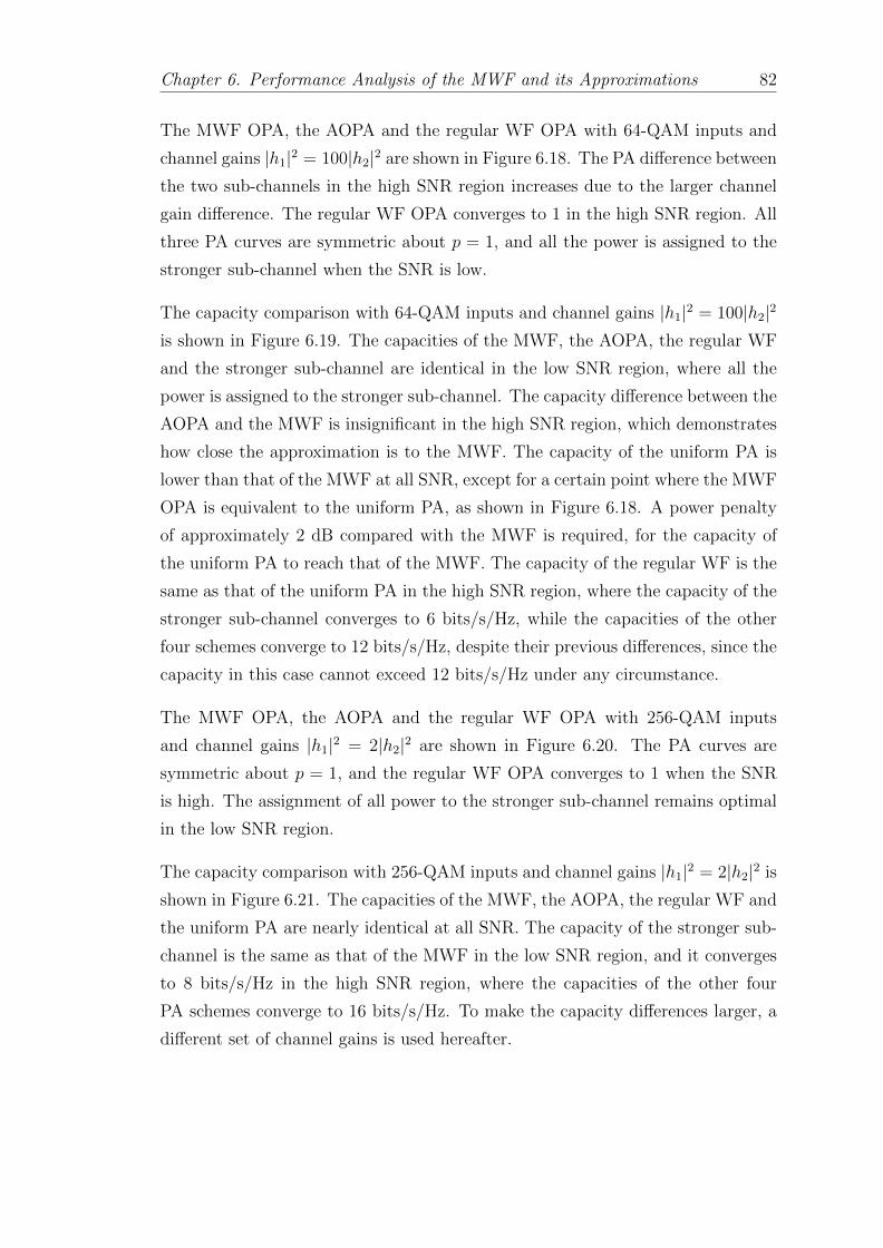
Chapter 6. Performance Analysis of the MWF and its Approximations 82
The MWF OPA, the AOPA and the regular WF OPA with 64-QAM inputs and
channel gains |h1|2 = 100|h2|2 are shown in Figure 6.18. The PA difference between
the two sub-channels in the high SNR region increases due to the larger channel
gain difference. The regular WF OPA converges to 1 in the high SNR region. All
three PA curves are symmetric about p = 1, and all the power is assigned to the
stronger sub-channel when the SNR is low.
The capacity comparison with 64-QAM inputs and channel gains |h1|2 = 100|h2|2
is shown in Figure 6.19. The capacities of the MWF, the AOPA, the regular WF
and the stronger sub-channel are identical in the low SNR region, where all the
power is assigned to the stronger sub-channel. The capacity difference between the
AOPA and the MWF is insignificant in the high SNR region, which demonstrates
how close the approximation is to the MWF. The capacity of the uniform PA is
lower than that of the MWF at all SNR, except for a certain point where the MWF
OPA is equivalent to the uniform PA, as shown in Figure 6.18. A power penalty
of approximately 2 dB compared with the MWF is required, for the capacity of
the uniform PA to reach that of the MWF. The capacity of the regular WF is the
same as that of the uniform PA in the high SNR region, where the capacity of the
stronger sub-channel converges to 6 bits/s/Hz, while the capacities of the other
four schemes converge to 12 bits/s/Hz, despite their previous differences, since the
capacity in this case cannot exceed 12 bits/s/Hz under any circumstance.
The MWF OPA, the AOPA and the regular WF OPA with 256-QAM inputs
and channel gains |h1|2 = 2|h2|2 are shown in Figure 6.20. The PA curves are
symmetric about p = 1, and the regular WF OPA converges to 1 when the SNR
is high. The assignment of all power to the stronger sub-channel remains optimal
in the low SNR region.
The capacity comparison with 256-QAM inputs and channel gains |h1|2 = 2|h2|2 is
shown in Figure 6.21. The capacities of the MWF, the AOPA, the regular WF and
the uniform PA are nearly identical at all SNR. The capacity of the stronger sub-
channel is the same as that of the MWF in the low SNR region, and it converges
to 8 bits/s/Hz in the high SNR region, where the capacities of the other four
PA schemes converge to 16 bits/s/Hz. To make the capacity differences larger, a
different set of channel gains is used hereafter.
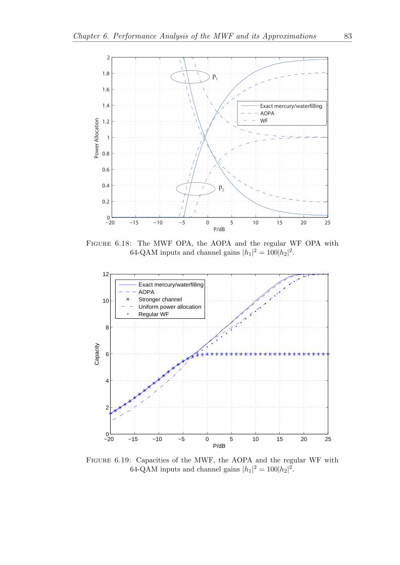
Chapter 6. Performance Analysis of the MWF and its Approximations 83
−20 −15 −10 −5 0 5 10 15 20 250
0.2
0.4
0.6
0.8
1
1.2
1.4
1.6
1.8
2
P/dB
Po
we
r A
lloca
tio
n
Exact mercury/waterfilling
AOPA
WF
p1
p2
Figure 6.18: The MWF OPA, the AOPA and the regular WF OPA with64-QAM inputs and channel gains |h1|2 = 100|h2|2.
−20 −15 −10 −5 0 5 10 15 20 250
2
4
6
8
10
12
P/dB
Cap
acity
Exact mercury/waterfillingAOPAStronger channelUniform power allocationRegular WF
Figure 6.19: Capacities of the MWF, the AOPA and the regular WF with64-QAM inputs and channel gains |h1|2 = 100|h2|2.
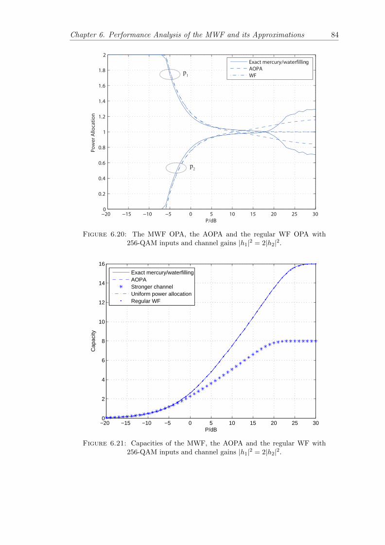
Chapter 6. Performance Analysis of the MWF and its Approximations 84
−20 −15 −10 −5 0 5 10 15 20 25 300
0.2
0.4
0.6
0.8
1
1.2
1.4
1.6
1.8
2
P/dB
Po
we
r A
lloca
tio
n
Exact mercury/waterfilling
AOPA
WFp1
p2
Figure 6.20: The MWF OPA, the AOPA and the regular WF OPA with256-QAM inputs and channel gains |h1|2 = 2|h2|2.
−20 −15 −10 −5 0 5 10 15 20 25 300
2
4
6
8
10
12
14
16
P/dB
Cap
acity
Exact mercury/waterfillingAOPAStronger channelUniform power allocationRegular WF
Figure 6.21: Capacities of the MWF, the AOPA and the regular WF with256-QAM inputs and channel gains |h1|2 = 2|h2|2.
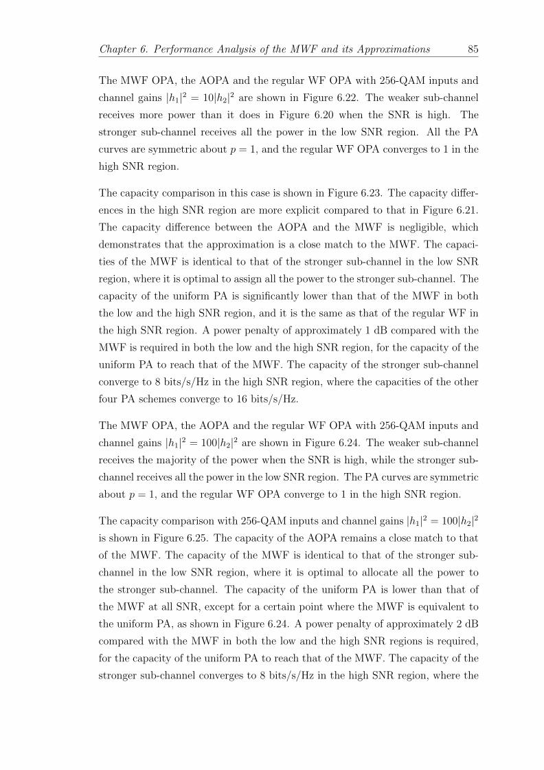
Chapter 6. Performance Analysis of the MWF and its Approximations 85
The MWF OPA, the AOPA and the regular WF OPA with 256-QAM inputs and
channel gains |h1|2 = 10|h2|2 are shown in Figure 6.22. The weaker sub-channel
receives more power than it does in Figure 6.20 when the SNR is high. The
stronger sub-channel receives all the power in the low SNR region. All the PA
curves are symmetric about p = 1, and the regular WF OPA converges to 1 in the
high SNR region.
The capacity comparison in this case is shown in Figure 6.23. The capacity differ-
ences in the high SNR region are more explicit compared to that in Figure 6.21.
The capacity difference between the AOPA and the MWF is negligible, which
demonstrates that the approximation is a close match to the MWF. The capaci-
ties of the MWF is identical to that of the stronger sub-channel in the low SNR
region, where it is optimal to assign all the power to the stronger sub-channel. The
capacity of the uniform PA is significantly lower than that of the MWF in both
the low and the high SNR region, and it is the same as that of the regular WF in
the high SNR region. A power penalty of approximately 1 dB compared with the
MWF is required in both the low and the high SNR region, for the capacity of the
uniform PA to reach that of the MWF. The capacity of the stronger sub-channel
converge to 8 bits/s/Hz in the high SNR region, where the capacities of the other
four PA schemes converge to 16 bits/s/Hz.
The MWF OPA, the AOPA and the regular WF OPA with 256-QAM inputs and
channel gains |h1|2 = 100|h2|2 are shown in Figure 6.24. The weaker sub-channel
receives the majority of the power when the SNR is high, while the stronger sub-
channel receives all the power in the low SNR region. The PA curves are symmetric
about p = 1, and the regular WF OPA converge to 1 in the high SNR region.
The capacity comparison with 256-QAM inputs and channel gains |h1|2 = 100|h2|2
is shown in Figure 6.25. The capacity of the AOPA remains a close match to that
of the MWF. The capacity of the MWF is identical to that of the stronger sub-
channel in the low SNR region, where it is optimal to allocate all the power to
the stronger sub-channel. The capacity of the uniform PA is lower than that of
the MWF at all SNR, except for a certain point where the MWF is equivalent to
the uniform PA, as shown in Figure 6.24. A power penalty of approximately 2 dB
compared with the MWF in both the low and the high SNR regions is required,
for the capacity of the uniform PA to reach that of the MWF. The capacity of the
stronger sub-channel converges to 8 bits/s/Hz in the high SNR region, where the
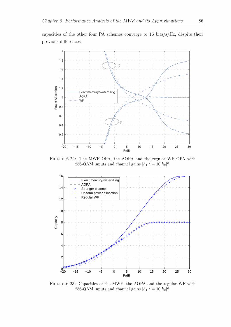
Chapter 6. Performance Analysis of the MWF and its Approximations 86
capacities of the other four PA schemes converge to 16 bits/s/Hz, despite their
previous differences.
−20 −15 −10 −5 0 5 10 15 20 25 300
0.2
0.4
0.6
0.8
1
1.2
1.4
1.6
1.8
2
P/dB
Po
we
r A
lloca
tio
n
Exact mercury/waterfilling
AOPA
WF
p1
p2
Figure 6.22: The MWF OPA, the AOPA and the regular WF OPA with256-QAM inputs and channel gains |h1|2 = 10|h2|2.
−20 −15 −10 −5 0 5 10 15 20 25 300
2
4
6
8
10
12
14
16
P/dB
Cap
acity
Exact mercury/waterfillingAOPAStronger channelUniform power allocationRegular WF
Figure 6.23: Capacities of the MWF, the AOPA and the regular WF with256-QAM inputs and channel gains |h1|2 = 10|h2|2.
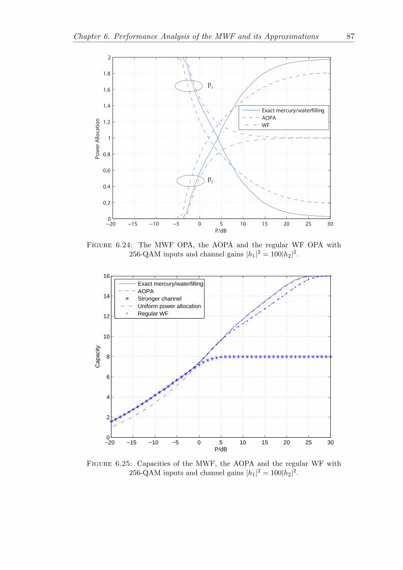
Chapter 6. Performance Analysis of the MWF and its Approximations 87
−20 −15 −10 −5 0 5 10 15 20 25 300
0.2
0.4
0.6
0.8
1
1.2
1.4
1.6
1.8
2
P/dB
Po
we
r A
lloca
tio
n
Exact mercury/waterfilling
AOPA
WF
p1
p2
Figure 6.24: The MWF OPA, the AOPA and the regular WF OPA with256-QAM inputs and channel gains |h1|2 = 100|h2|2.
−20 −15 −10 −5 0 5 10 15 20 25 300
2
4
6
8
10
12
14
16
P/dB
Cap
acity
Exact mercury/waterfillingAOPAStronger channelUniform power allocationRegular WF
Figure 6.25: Capacities of the MWF, the AOPA and the regular WF with256-QAM inputs and channel gains |h1|2 = 100|h2|2.
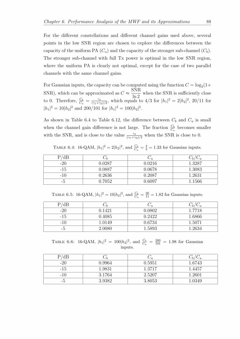
Chapter 6. Performance Analysis of the MWF and its Approximations 88
For the different constellations and different channel gains used above, several
points in the low SNR region are chosen to explore the differences between the
capacity of the uniform PA (Cu) and the capacity of the stronger sub-channel (Cb).
The stronger sub-channel with full Tx power is optimal in the low SNR region,
where the uniform PA is clearly not optimal, except for the case of two parallel
channels with the same channel gains.
For Gaussian inputs, the capacity can be computed using the function C = log2(1+
SNR), which can be approximated as C ≈ SNR
ln 2when the SNR is sufficiently close
to 0. Therefore, CbCu
= γ1(γ1+γ2)/2
, which equals to 4/3 for |h1|2 = 2|h2|2, 20/11 for
|h1|2 = 10|h2|2 and 200/101 for |h1|2 = 100|h2|2.
As shown in Table 6.4 to Table 6.12, the difference between Cb and Cu is small
when the channel gain difference is not large. The fraction CbCu
becomes smaller
with the SNR, and is close to the value γ1(γ1+γ2)/2
when the SNR is close to 0.
Table 6.4: 16-QAM, |h1|2 = 2|h2|2, and CbCu
= 43 = 1.33 for Gaussian inputs.
P/dB Cb Cu Cb/Cu-20 0.0287 0.0216 1.3287-15 0.0887 0.0678 1.3083-10 0.2636 0.2087 1.2631-5 0.7052 0.6097 1.1566
Table 6.5: 16-QAM, |h1|2 = 10|h2|2, and CbCu
= 2011 = 1.82 for Gaussian inputs.
P/dB Cb Cu Cb/Cu-20 0.1421 0.0802 1.7718-15 0.4085 0.2422 1.6866-10 1.0149 0.6734 1.5071-5 2.0080 1.5893 1.2634
Table 6.6: 16-QAM, |h1|2 = 100|h2|2, and CbCu
= 200101 = 1.98 for Gaussian
inputs.
P/dB Cb Cu Cb/Cu-20 0.9964 0.5951 1.6743-15 1.9831 1.3717 1.4457-10 3.1764 2.5207 1.2601-5 3.9382 3.8053 1.0349
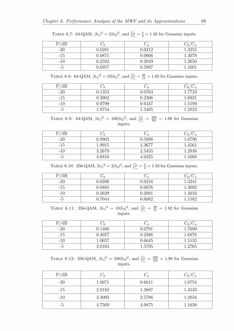
Chapter 6. Performance Analysis of the MWF and its Approximations 89
Table 6.7: 64-QAM, |h1|2 = 2|h2|2, and CbCu
= 43 = 1.33 for Gaussian inputs.
P/dB Cb Cu Cb/Cu-20 0.0281 0.0212 1.3255-15 0.0871 0.0666 1.3078-10 0.2592 0.2049 1.2650-5 0.6957 0.5997 1.1601
Table 6.8: 64-QAM, |h1|2 = 10|h2|2, and CbCu
= 2011 = 1.82 for Gaussian inputs.
P/dB Cb Cu Cb/Cu-20 0.1353 0.0763 1.7733-15 0.3902 0.2306 1.6921-10 0.9799 0.6447 1.5199-5 1.9754 1.5405 1.2823
Table 6.9: 64-QAM, |h1|2 = 100|h2|2, and CbCu
= 200101 = 1.98 for Gaussian
inputs.
P/dB Cb Cu Cb/Cu-20 0.9903 0.5898 1.6790-15 1.9915 1.3677 1.4561-10 3.2679 2.5455 1.2838-5 4.6810 4.0325 1.1608
Table 6.10: 256-QAM, |h1|2 = 2|h2|2, and CbCu
= 43 = 1.33 for Gaussian inputs.
P/dB Cb Cu Cb/Cu-20 0.0286 0.0216 1.3241-15 0.0885 0.0676 1.3092-10 0.2629 0.2081 1.2633-5 0.7044 0.6082 1.1582
Table 6.11: 256-QAM, |h1|2 = 10|h2|2, and CbCu
= 2011 = 1.82 for Gaussian
inputs.
P/dB Cb Cu Cb/Cu-20 0.1400 0.0791 1.7699-15 0.4027 0.2386 1.6878-10 1.0057 0.6645 1.5135-5 2.0163 1.5795 1.2765
Table 6.12: 256-QAM, |h1|2 = 100|h2|2, and CbCu
= 200101 = 1.98 for Gaussian
inputs.
P/dB Cb Cu Cb/Cu
-20 1.0071 0.6011 1.6754
-15 2.0182 1.3887 1.4533
-10 3.3093 2.5786 1.2834
-5 4.7569 4.0875 1.1638
Chapter 6. Performance Analysis of the MWF and its Approximations 90
6.2 Three Parallel Channels
The case of three parallel channels is explored in comparison with that of two
parallel channels. The setting is similar to that of two parallel channels, where two
sets of channel gains, i.e., |h1|2 = 2|h2|2 = 4|h3|2 and |h1|2 = 10|h2|2 = 100|h3|2,are used. The normalized power constraint is p∗1 + p∗2 + p∗3 = 3, under which the
constellations 4-QAM, 16-QAM and 64-QAM are used.
The MWF OPA and the AOPA with 4-QAM inputs and channel gains |h1|2 =
2|h2|2 = 4|h3|2 are shown in Figure 6.26. Channels 2 and 3 are inactive initially
in the low SNR region due to their low channel gains, but they become active as
the SNR increases. The turning points on the curves are due to the activation
of inactive channels. The difference between the MWF OPA and the AOPA is
significant in the high SNR region, however, the difference does not affect capacity
greatly. Unlike the case of two parellel channels, the curves are not symmetric,
and they do not cross at p = 1.
The capacity comparison between different PA schemes with 4-QAM inputs and
channel gains |h1|2 = 2|h2|2 = 4|h3|2 is shown in Figure 6.27. The capacity of the
uniform PA is lower than that of the MWF in both the low and the high SNR
region, and it has an approximately 1 dB power penalty compared with the MWF.
The capacity of the MWF is identical to that of the strongest sub-channel in the
low SNR region, where it is optimal to allocate all the power to the strongest
sub-channel. However, the capacity of the strongest sub-channel converges to 2
bits/s/Hz in the high SNR region, where the capacities of the other three schemes
converge to 6 bits/s/Hz. The capacity difference between the MWF and the AOPA
is negligible, which shows that the approximation is a close match to the MWF.

Chapter 6. Performance Analysis of the MWF and its Approximations 91
−20 −15 −10 −5 0 5 10 150
0.5
1
1.5
2
2.5
3
P/dB
Po
we
r A
lloca
tio
n
Exact mercury/waterfilling
AOPA
p1
p3
p2
Figure 6.26: The MWF OPA and the AOPA with 4-QAM inputs and channelgains |h1|2 = 2|h2|2 = 4|h3|2.
−20 −15 −10 −5 0 5 10 150
1
2
3
4
5
6
P/dB
Cap
acity
Exact mercury/waterfillingAOPAStronger channelUniform power allocation
Figure 6.27: Capacities of the MWF and the AOPA with 4-QAM inputs andchannel gains |h1|2 = 2|h2|2 = 4|h3|2.
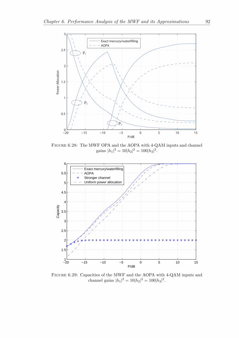
Chapter 6. Performance Analysis of the MWF and its Approximations 92
−20 −15 −10 −5 0 5 10 150
0.5
1
1.5
2
2.5
3
P/dB
Po
we
r A
lloca
tio
n
Exact mercury/waterfilling
AOPA
p1
p3
p2
Figure 6.28: The MWF OPA and the AOPA with 4-QAM inputs and channelgains |h1|2 = 10|h2|2 = 100|h3|2.
−20 −15 −10 −5 0 5 10 151
1.5
2
2.5
3
3.5
4
4.5
5
5.5
6
P/dB
Cap
acity
Exact mercury/waterfillingAOPAStronger channelUniform power allocation
Figure 6.29: Capacities of the MWF and the AOPA with 4-QAM inputs andchannel gains |h1|2 = 10|h2|2 = 100|h3|2.
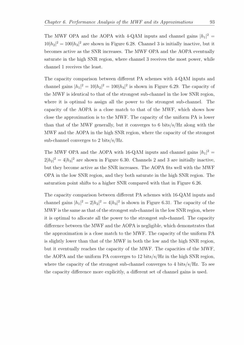
Chapter 6. Performance Analysis of the MWF and its Approximations 93
The MWF OPA and the AOPA with 4-QAM inputs and channel gains |h1|2 =
10|h2|2 = 100|h3|2 are shown in Figure 6.28. Channel 3 is initially inactive, but it
becomes active as the SNR increases. The MWF OPA and the AOPA eventually
saturate in the high SNR region, where channel 3 receives the most power, while
channel 1 receives the least.
The capacity comparison between different PA schemes with 4-QAM inputs and
channel gains |h1|2 = 10|h2|2 = 100|h3|2 is shown in Figure 6.29. The capacity of
the MWF is identical to that of the strongest sub-channel in the low SNR region,
where it is optimal to assign all the power to the strongest sub-channel. The
capacity of the AOPA is a close match to that of the MWF, which shows how
close the approximation is to the MWF. The capacity of the uniform PA is lower
than that of the MWF generally, but it converges to 6 bits/s/Hz along with the
MWF and the AOPA in the high SNR region, where the capacity of the strongest
sub-channel converges to 2 bits/s/Hz.
The MWF OPA and the AOPA with 16-QAM inputs and channel gains |h1|2 =
2|h2|2 = 4|h3|2 are shown in Figure 6.30. Channels 2 and 3 are initially inactive,
but they become active as the SNR increases. The AOPA fits well with the MWF
OPA in the low SNR region, and they both saturate in the high SNR region. The
saturation point shifts to a higher SNR compared with that in Figure 6.26.
The capacity comparison between different PA schemes with 16-QAM inputs and
channel gains |h1|2 = 2|h2|2 = 4|h3|2 is shown in Figure 6.31. The capacity of the
MWF is the same as that of the strongest sub-channel in the low SNR region, where
it is optimal to allocate all the power to the strongest sub-channel. The capacity
difference between the MWF and the AOPA is negligible, which demonstrates that
the approximation is a close match to the MWF. The capacity of the uniform PA
is slightly lower than that of the MWF in both the low and the high SNR region,
but it eventually reaches the capacity of the MWF. The capacities of the MWF,
the AOPA and the uniform PA converges to 12 bits/s/Hz in the high SNR region,
where the capacity of the strongest sub-channel converges to 4 bits/s/Hz. To see
the capacity difference more explicitly, a different set of channel gains is used.
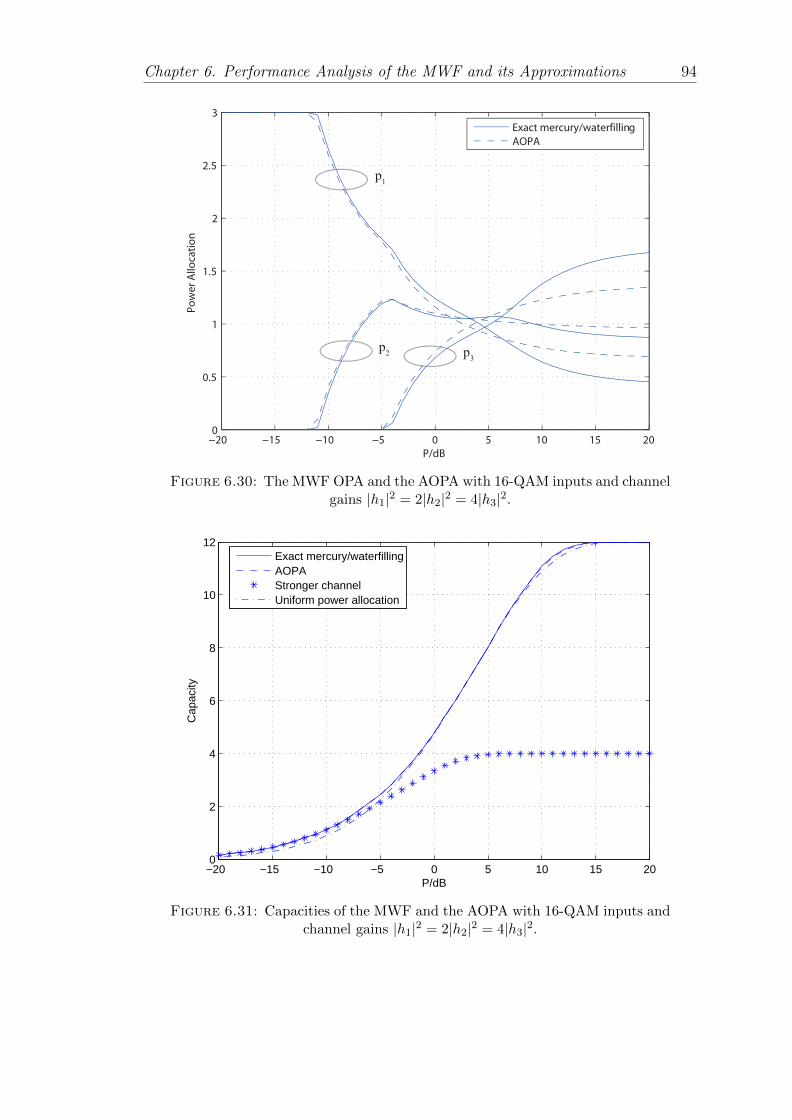
Chapter 6. Performance Analysis of the MWF and its Approximations 94
−20 −15 −10 −5 0 5 10 15 200
0.5
1
1.5
2
2.5
3
P/dB
Po
we
r A
lloca
tio
n
Exact mercury/waterfilling
AOPA
p1
p3
p2
Figure 6.30: The MWF OPA and the AOPA with 16-QAM inputs and channelgains |h1|2 = 2|h2|2 = 4|h3|2.
−20 −15 −10 −5 0 5 10 15 200
2
4
6
8
10
12
P/dB
Cap
acity
Exact mercury/waterfillingAOPAStronger channelUniform power allocation
Figure 6.31: Capacities of the MWF and the AOPA with 16-QAM inputs andchannel gains |h1|2 = 2|h2|2 = 4|h3|2.
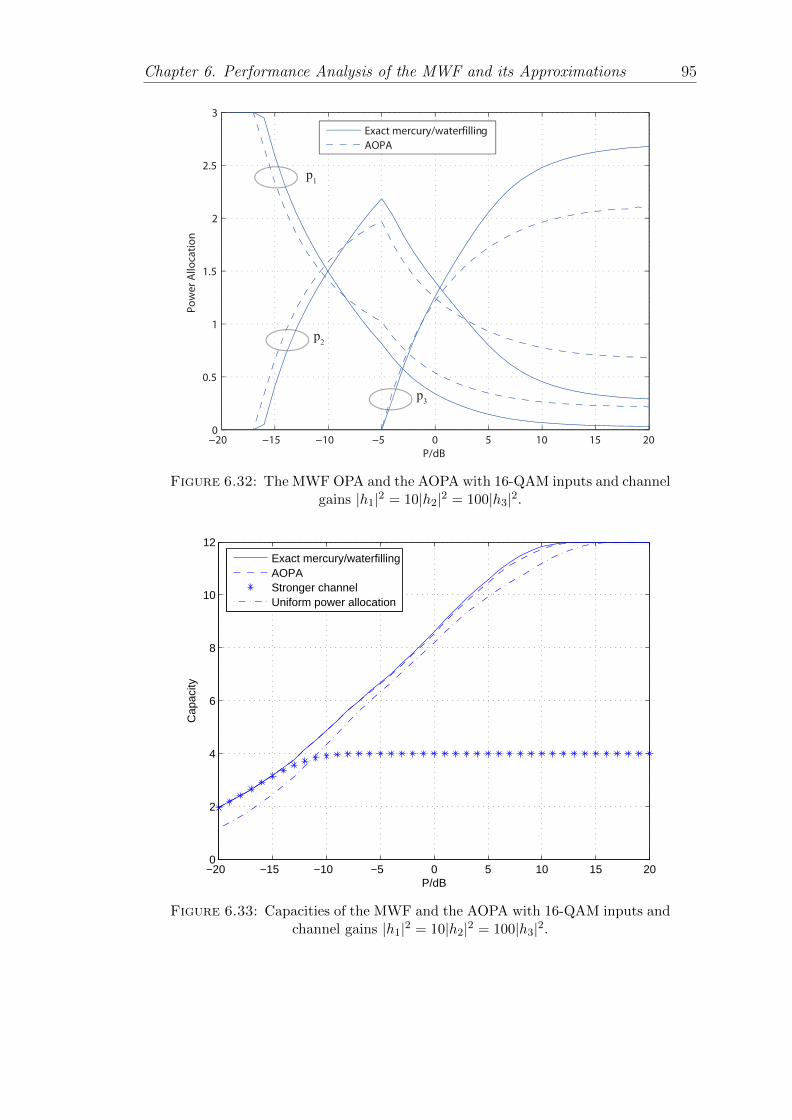
Chapter 6. Performance Analysis of the MWF and its Approximations 95
−20 −15 −10 −5 0 5 10 15 200
0.5
1
1.5
2
2.5
3
P/dB
Po
we
r A
lloca
tio
n
Exact mercury/waterfilling
AOPA
p1
p3
p2
Figure 6.32: The MWF OPA and the AOPA with 16-QAM inputs and channelgains |h1|2 = 10|h2|2 = 100|h3|2.
−20 −15 −10 −5 0 5 10 15 200
2
4
6
8
10
12
P/dB
Cap
acity
Exact mercury/waterfillingAOPAStronger channelUniform power allocation
Figure 6.33: Capacities of the MWF and the AOPA with 16-QAM inputs andchannel gains |h1|2 = 10|h2|2 = 100|h3|2.
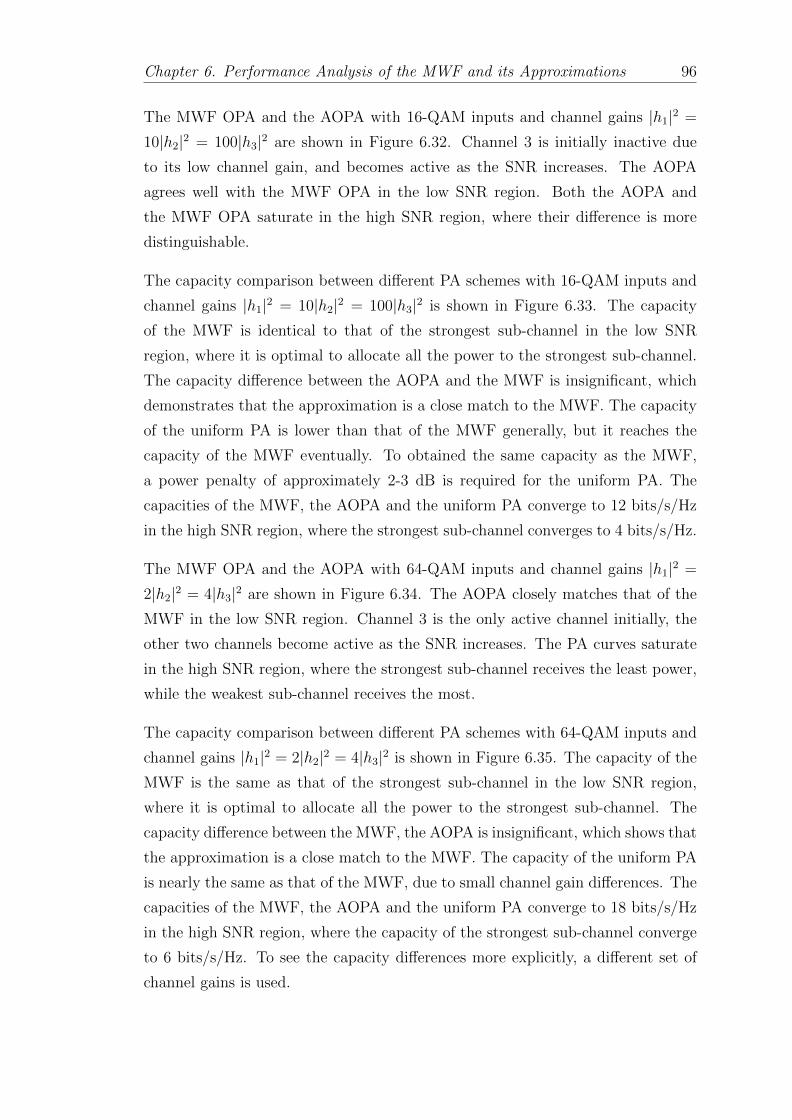
Chapter 6. Performance Analysis of the MWF and its Approximations 96
The MWF OPA and the AOPA with 16-QAM inputs and channel gains |h1|2 =
10|h2|2 = 100|h3|2 are shown in Figure 6.32. Channel 3 is initially inactive due
to its low channel gain, and becomes active as the SNR increases. The AOPA
agrees well with the MWF OPA in the low SNR region. Both the AOPA and
the MWF OPA saturate in the high SNR region, where their difference is more
distinguishable.
The capacity comparison between different PA schemes with 16-QAM inputs and
channel gains |h1|2 = 10|h2|2 = 100|h3|2 is shown in Figure 6.33. The capacity
of the MWF is identical to that of the strongest sub-channel in the low SNR
region, where it is optimal to allocate all the power to the strongest sub-channel.
The capacity difference between the AOPA and the MWF is insignificant, which
demonstrates that the approximation is a close match to the MWF. The capacity
of the uniform PA is lower than that of the MWF generally, but it reaches the
capacity of the MWF eventually. To obtained the same capacity as the MWF,
a power penalty of approximately 2-3 dB is required for the uniform PA. The
capacities of the MWF, the AOPA and the uniform PA converge to 12 bits/s/Hz
in the high SNR region, where the strongest sub-channel converges to 4 bits/s/Hz.
The MWF OPA and the AOPA with 64-QAM inputs and channel gains |h1|2 =
2|h2|2 = 4|h3|2 are shown in Figure 6.34. The AOPA closely matches that of the
MWF in the low SNR region. Channel 3 is the only active channel initially, the
other two channels become active as the SNR increases. The PA curves saturate
in the high SNR region, where the strongest sub-channel receives the least power,
while the weakest sub-channel receives the most.
The capacity comparison between different PA schemes with 64-QAM inputs and
channel gains |h1|2 = 2|h2|2 = 4|h3|2 is shown in Figure 6.35. The capacity of the
MWF is the same as that of the strongest sub-channel in the low SNR region,
where it is optimal to allocate all the power to the strongest sub-channel. The
capacity difference between the MWF, the AOPA is insignificant, which shows that
the approximation is a close match to the MWF. The capacity of the uniform PA
is nearly the same as that of the MWF, due to small channel gain differences. The
capacities of the MWF, the AOPA and the uniform PA converge to 18 bits/s/Hz
in the high SNR region, where the capacity of the strongest sub-channel converge
to 6 bits/s/Hz. To see the capacity differences more explicitly, a different set of
channel gains is used.
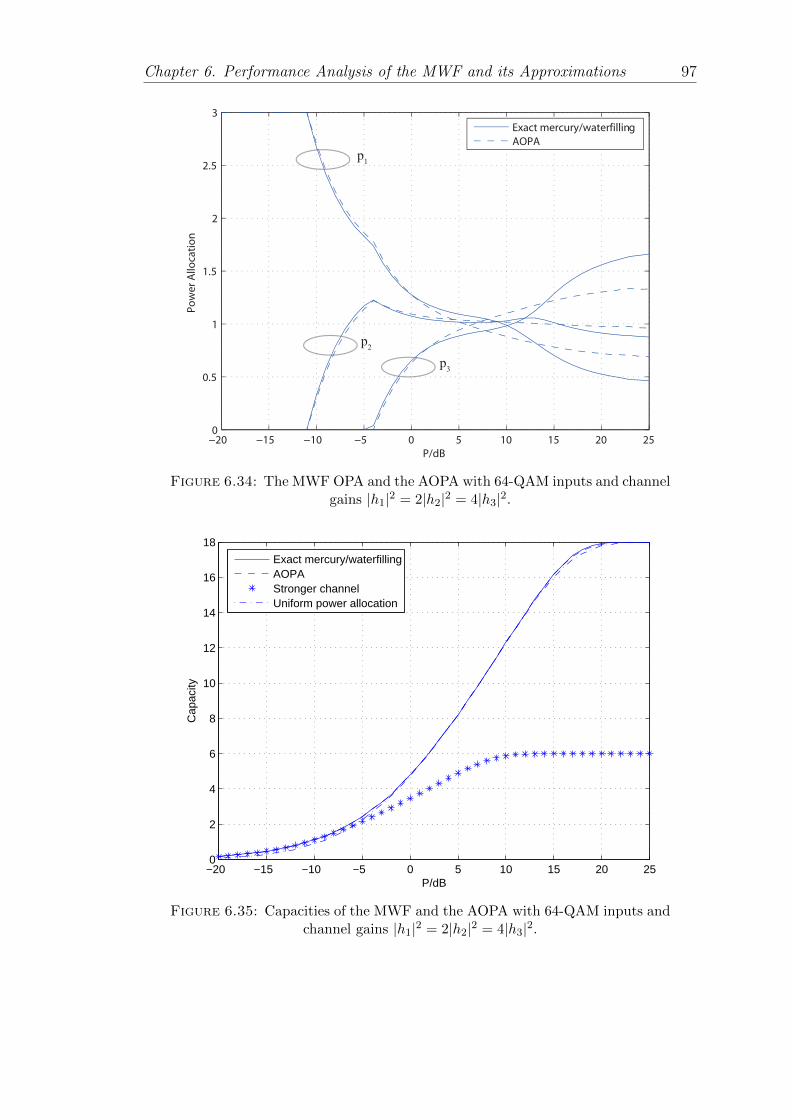
Chapter 6. Performance Analysis of the MWF and its Approximations 97
−20 −15 −10 −5 0 5 10 15 20 250
0.5
1
1.5
2
2.5
3
P/dB
Po
we
r A
lloca
tio
n
Exact mercury/waterfilling
AOPA
p1
p3
p2
Figure 6.34: The MWF OPA and the AOPA with 64-QAM inputs and channelgains |h1|2 = 2|h2|2 = 4|h3|2.
−20 −15 −10 −5 0 5 10 15 20 250
2
4
6
8
10
12
14
16
18
P/dB
Cap
acity
Exact mercury/waterfillingAOPAStronger channelUniform power allocation
Figure 6.35: Capacities of the MWF and the AOPA with 64-QAM inputs andchannel gains |h1|2 = 2|h2|2 = 4|h3|2.
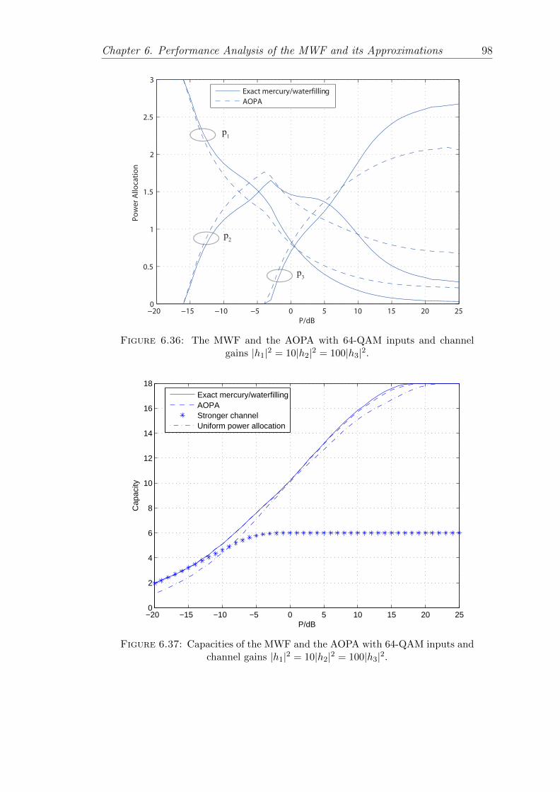
Chapter 6. Performance Analysis of the MWF and its Approximations 98
−20 −15 −10 −5 0 5 10 15 20 250
0.5
1
1.5
2
2.5
3
P/dB
Po
we
r A
lloca
tio
n
Exact mercury/waterfilling
AOPA
p1
p3
p2
Figure 6.36: The MWF and the AOPA with 64-QAM inputs and channelgains |h1|2 = 10|h2|2 = 100|h3|2.
−20 −15 −10 −5 0 5 10 15 20 250
2
4
6
8
10
12
14
16
18
P/dB
Cap
acity
Exact mercury/waterfillingAOPAStronger channelUniform power allocation
Figure 6.37: Capacities of the MWF and the AOPA with 64-QAM inputs andchannel gains |h1|2 = 10|h2|2 = 100|h3|2.
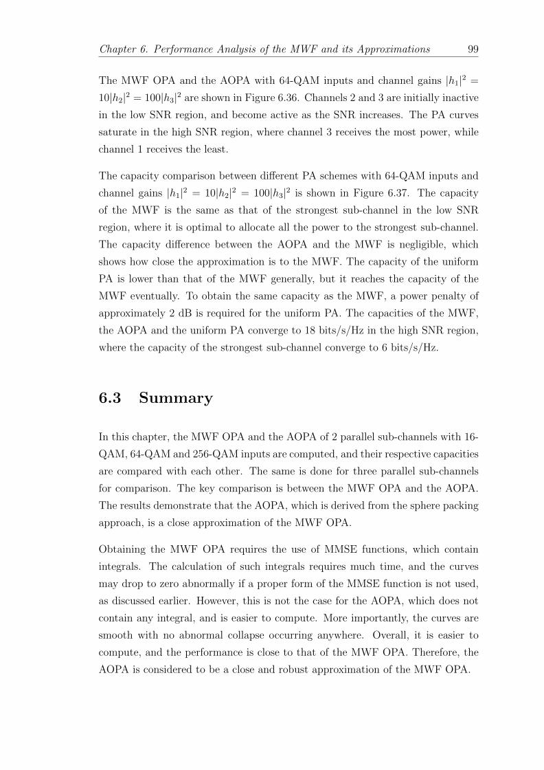
Chapter 6. Performance Analysis of the MWF and its Approximations 99
The MWF OPA and the AOPA with 64-QAM inputs and channel gains |h1|2 =
10|h2|2 = 100|h3|2 are shown in Figure 6.36. Channels 2 and 3 are initially inactive
in the low SNR region, and become active as the SNR increases. The PA curves
saturate in the high SNR region, where channel 3 receives the most power, while
channel 1 receives the least.
The capacity comparison between different PA schemes with 64-QAM inputs and
channel gains |h1|2 = 10|h2|2 = 100|h3|2 is shown in Figure 6.37. The capacity
of the MWF is the same as that of the strongest sub-channel in the low SNR
region, where it is optimal to allocate all the power to the strongest sub-channel.
The capacity difference between the AOPA and the MWF is negligible, which
shows how close the approximation is to the MWF. The capacity of the uniform
PA is lower than that of the MWF generally, but it reaches the capacity of the
MWF eventually. To obtain the same capacity as the MWF, a power penalty of
approximately 2 dB is required for the uniform PA. The capacities of the MWF,
the AOPA and the uniform PA converge to 18 bits/s/Hz in the high SNR region,
where the capacity of the strongest sub-channel converge to 6 bits/s/Hz.
6.3 Summary
In this chapter, the MWF OPA and the AOPA of 2 parallel sub-channels with 16-
QAM, 64-QAM and 256-QAM inputs are computed, and their respective capacities
are compared with each other. The same is done for three parallel sub-channels
for comparison. The key comparison is between the MWF OPA and the AOPA.
The results demonstrate that the AOPA, which is derived from the sphere packing
approach, is a close approximation of the MWF OPA.
Obtaining the MWF OPA requires the use of MMSE functions, which contain
integrals. The calculation of such integrals requires much time, and the curves
may drop to zero abnormally if a proper form of the MMSE function is not used,
as discussed earlier. However, this is not the case for the AOPA, which does not
contain any integral, and is easier to compute. More importantly, the curves are
smooth with no abnormal collapse occurring anywhere. Overall, it is easier to
compute, and the performance is close to that of the MWF OPA. Therefore, the
AOPA is considered to be a close and robust approximation of the MWF OPA.
Chapter 7
Conclusion
7.1 Thesis Summary
The digital transmission system is introduced with a block diagram. The three
blocks, modulation, channel and demodulation are considered as an extended chan-
nel. For such extended channel, our objective is to find the OPA that maximizes
the capacity.
Channel capacity is presented, more specifically, the Gaussian channel capacity
and the constellation capacity. There is an integral inside the constellation ca-
pacity expression, which can not be evaluated analytically. The Moente Carlo
integration is used to evaluate it instead. The sphere packing argument is uti-
lized to obtain an approximation of the constellation capacity, since its original
expression is quite complicated.
Several OPA schemes and respective approximations are discussed. The regular
WF is optimal for Gaussian inputs, and the MWF is a generalized WF which is
optimal for arbitrary input distributions. An approximation of the MWF based
on the sphere packing argument is presented, which is called the constellation-
constrained WF (or AOPA). A parallel channel model is also introduced as the
context.
The MWF is based on MMSE functions. A general expression of the MMSE is pre-
sented, along with expressions for several specific constellations. The MWF turns
into the regular WF if the input is Gaussian. A high and a low power expansion
100
Chapter 7. Conclusion 101
of MMSE are discussed as well. A figure of MMSE for different constellations are
shown, which is identical to its counterpart in [1].
Several errors are found in [1]. More importantly, a loss of precision is found
during the simulation, due to the structure of the specific MMSE functions. The
limited precision of the numerical computation cannot give an accurate result in
this case. Therefore, the general expression of the MMSE function (3.21) is used
to obtain the MWF OPA instead.
A new algorithm, the internal/external bisection algorithm is developed in order
to obtain the MWF OPA. For such algorithm to start, upper and lower bounds
needs to be derived first, which change dynamically with respect to the SNR. The
internal bisecion is to obtain the MMSE−1(·), while the external one is to obtain
the value of η.
For the AOPA, the loss of precision is not a problem. The optimization problem
for the AOPA is a convex optimization problem, which can be solved via the
KKT conditions. The CVX was used initially, but problems arose in the process.
There are abnormal gaps on the PA curves, for which the ”cvx status” are failed.
Therefore, the AOPA is obtained via the bisection method in combination with
the total power constraint, since the AOPA is a monotonic function.
Capacities of different PA schemes are computed and compared with each other,
especially between the AOPA and the MWF. The setting of two parallel sub-
channels with 16-QAM, 64-QAM and 256-QAM inputs, and channel gains |h1|2 =
2|h2|2, |h1|2 = 10|h2|2 and |h1|2 = 100|h2|2 are utilized. The same is used for
three parallel sub-channels for comparison, with channel gains |h1|2 = 2|h2|2 =
4|h3|2, |h1|2 = 10|h2|2 = 100|h3|2. Several other PA schemes are used as well for
comparison, such as the regular WF, the uniform PA, the stronger sub-channel
with all the Tx power and the Monte Carlo OPA. The results demonstrate that
the AOPA is a close approximation of the MWF.
7.2 Future research
The work stated in the thesis could be expanded in several ways:
1. The same constellation is used on all the sub-channels for comparison purposes
in the thesis. However, a higher order constellation can be applied to the stronger
Chapter 7. Conclusion 102
sub-channel in the case of |h1|2 = 100|h2|2, so that the stronger sub-channel will
get more power at high SNR.
2. For the future 5G system, the enablers are better energy efficiency and higher
data rate. Our objective is to obtain the OPA that maximizes the capacity, which
correspond to the enablers above. We believe this work could be useful in the
upcoming new generation.
Appendix A
A.1 History from 1G to 5G
The basic concepts of wireless communication are addressed in [38], as well as
various technologies for 2G and 3G. 2G is a significant improvement compared to
1G, which is analog only. An important standard for 2G, GSM (Global System
for Mobile Communications), was developed by the European Telecommunications
Standards Institute. For GSM, the signals are digital instead of analog as in 1G.
A typical method for 2G is TDMA (Time Division Multiple Access), which allows
users to utilize the same channel at different time slots [39]. Currently, GSM is
still used to provide voice services due to the fact that it provides high quality
voice services at a reduced cost. More details about GSM systems for mobile
communications can be found in [40]. Unlike 2G, the later generations focus more
on data services, and numerous new technologies have been developed since then.
GPRS (General Packet Radio Service) is in between of 2G and 3G, which is usually
referred to as 2.5G. It provides data services along with the voice services provided
by GSM. It utilizes the unused TDMA channels in the GSM network, providing a
data rate of 56-114 kbps. More details about GPRS and its performance can be
found in [40].
The 3rd generation has a great improvement compared to 2G, with significantly
higher data rate. Its history and development can be found in [39]. The motivation
of 3G research is to seek for a higher data rate compared to 2G. There are a
number of new technologies for 3G, including CDMA (Code Division Multiple
Access), EDGE (Enhanced Data rates for GSM Evolution) and HSCSD (High-
Speed Circuit-Switched Data) [40] [41]. Performances of different standards are
discussed in [41] along with their backgrounds. CDMA is a channel access method,
103
Appendix 104
which has two variations: TD-CDMA (Time Division CDMA) and TD-SCDMA
(Time Division synchronous CDMA) [39]. TD-CDMA is a multiple access method
that is used on different time slots. TD-SCDMA is a multiple access method using
adaptive synchronous CDMA components, which is developed by China.
EDGE is also known as enhanced GPRS, which is an extension of GSM. It results
in an increased capacity and delivers higher rate compared to GPRS. HSCSD
utilizes a more efficient coding scheme, and uses several time slots at the same
time in order to achieve a higher rate. WAP (Wireless Application Protocol) is
a protocol that enables users to use wireless devices to connect to the internet at
any time, which makes it possible for mobile devices to use applications that are
similar to web browsers on computers [40].
LTE (Long term evolution) [42] is a standard for high-speed wireless communica-
tion, which is developed by 3GPP. It introduces several new technologies such as
OFDM (Orthogonal Frequency Division Multiplexing) [25] [30] and MIMO (Mul-
tiple Input Multiple Output) [43]. OFDM encodes data on multiple carrier fre-
quencies, it is able to deal with severe channel conditions such as fading. MIMO
deploys multiple antennas at both the transmitter and the receiver. The extra
antennas exploit multipath propagation between the transmitter and the receiver,
so that the channel capacity is greatly increased. Those technologies increase
the data rate and spectral efficiency considerably. An optimal power allocation
(OPA) for OFDM with arbitrary input distributions can be found in [30], and
multiuser mercury/waterfilling (MWF) for downlink OFDM can be found in [27].
As for MIMO, a popular detection algorithm to the receiver is V-BLAST (Vertical-
Bell Laboratories Layered Space-Time), which utilizes the spatial multiplexing of
MIMO systems. An OPA for V-BLAST can be found in [44] and an optimal
ordering for coded ZF (Zero Forcing) and MMSE V-BLAST is discussed in [45].
Optimal power and rate allocation for coded V-BLAST are discussed in [46] and
[47].
Channel capacity and coverage are increased significantly due to the fact that LTE
supports the mainstream frequency bands of 2G/3G and some other new ones. The
network of LTE systems is simplified, reducing the complexity of the system. As
a result, system delay and maintenance cost are reduced as well. LTE-Advanced
is an enhancement of LTE, which has higher throughput. Its performance is dis-
cussed in [42].
Appendix 105
The following generation will be 5G, of which extensive research has been initiated.
The goal of 5G is to satisfy the rising traffic volume, and to provide users with a
higher data rate and lower latency [48]. Overall, it creates a better user experience.
Therefore there are some specific properties that 5G should have, for instance,
high carrier frequencies, massive bandwidths, and highly integrative systems [48].
Several new technologies designed for 5G are discussed below.
Limitations of 4G include spectrum scarcity and high energy consumption. New
technologies are developed in order to deal with these issues, several of which are
discussed in [49]. Massive MIMO, millimeter wave and small cell are amongst
those key technologies, which form the basis of 5G. Massive MIMO is an evolution
of its predecessor, MIMO [50]. Within MIMO systems, more antennas are located
at both the transmitter and reciever, which create more signal paths and achieve
higher capacity in return. Massive MIMO is more effective due to the excessive
number of antennas it has. It confines transmit and receive signal energy within
a small area, throughput and energy efficiency receives a huge improvement as
a result. Massive MIMO provides a higher capacity, lower latency and better
coverage for the system, which are crucial to user experience. However, some issues
still exist and need to be addressed, which include the high cost of deploying all
the antennas, maintenance fees and the cost of channel estimation and feedback
[50]. Despite the issues above, massive MIMO is one of the enabling technologies
for 5G with bright future.
Millimeter wave is another key technology of 5G that exploits untapped higher
frequency bands. Lower frequency bands are currently crowded due to the fact
that they are where most of the current communication systems operate. The
bandwidth shortage makes it essential to utilize higher frequencies beyond. A
millimeter wave solution for 5G is introduced in [51], which can be used in the
upcoming 5G system. For higher frequencies, 28 GHz and 38 GHz can be used
when employing steerable directional antennas at base stations and mobile devices.
More details can be found in [51].
Small cell works at a designated frequency band with low power consumption. It
is small compared to Macrocell, and covers a shorter range of 10 to 200 meters.
There are several kinds of small cells, such as Femtocell, Picocell and Microcells.
Small cell makes it possible to reuse the same frequency band multiple times, so
that the capacity and spectral efficiency are increased greatly [52]. As a result,
better user experience is obtained with higher data rate and lower latency. Small
Appendix 106
cell designs can be found in [52]. However, the inter-cell interference is a challenge
which needs to be properly dealt with [53].
Small cell systems can also be connected to cellular networks to create a heteroge-
neous network, which also increases network capacity and spectral efficiency [52].
Heterogeneous network, also known as HetNet, is a type of network architecture
that consists of small cells connecting different types of base stations, such as
Femto-, Pico- and Marcocells [53]. HetNet is a key idea for future network devel-
opment, and it will satisfy the rising traffic volume once the inter-cell interference
problem is solved.
A.2 Proof of Theorem 3.2
Mutual information I(piγi) is known to be a concave function, therefore its maxi-
mization is identical to the minimization of −I(piγi), which is a convex function. It
is a convex optimization problem and the OPA can be solved via KKT conditions.
The standard form of convex optimization problems is as follows [35]:
minimize f0(x) (A.1)
subject to fi(x) ≤ 0, i = 1, ...,m (A.2)
hi(x) = 0, i = 1, ..., p (A.3)
where f0, f1, ..., fm are convex functions, and hi is affine.
KKT conditions represent a method of solving convex optimization problems, the
following four conditions are called KKT conditions (with differentiable fi, hi):
1. Primal Constraints: fi(x) ≤ 0, i = 1, ...,m, hi(x) = 0, i = 1, ..., p.
2. Dual Constraints: λi ≥ 0.
3. Complementary Slackness: λifi(x) = 0, i = 1, ...,m.
4. Gradient of Lagrangian with respect to x vanishes:
∇f0(x) +m∑i=1
λi∇fi(x) +
p∑i=1
ηi∇hi(x) = 0 (A.4)
Appendix 107
According to (3.6), the optimization problem can be written as
min−∑
I(piγi) (A.5)
subject to pi ≥ 0 (A.6)∑pi = n (A.7)
The Lagrangian can be written as:
L = −∑
I(piγi)−∑
λipi + η(∑
pi − n)
(A.8)
Thus the KKT conditions for the OPA problem are:
∂L
∂pi= −γiMMSE(piγi) + η − λi = 0 (A.9)
λipi = 0 (A.10)
λi ≥ 0 (A.11)
pi ≥ 0 (A.12)
The gradient of the Lagrangian in (A.9) can be further simplified as:
pi =1
γiMMSE−1
(η − λiγi
)(A.13)
The complementary slackness (A.10) can be divided into two different scenarios
as follows:
1. pi > 0, λi = 0
Substitute (A.13) into the inequality:
1
γiMMSE−1
(η − λiγi
)> 0 (A.14)
Due to the fact that MMSE−1(·) is a monotonically decreasing function, and
MMSE−1(1) = 0, (A.14) turns into
η − λiγi
< 1 (A.15)
Appendix 108
where λi = 0 in this case. The inequality η < γi can be derived from (A.15). From
(A.13), p∗i is retrieved for this scenario:
p∗i =1
γiMMSE−1
(η
γi
)(A.16)
2. pi = 0, λi ≥ 0
Substitute (A.13) into the equality:
1
γiMMSE−1
(η − λiγi
)= 0 (A.17)
where MMSE−1(1) = 0, therefore (A.17) turns into
η = λi + γi (A.18)
with λi ≥ 0 for this scenario, it is obvious that η ≥ γi. Therefore the OPA is
p∗i = 0.
With the two scenarios combined, the OPA is
p∗i = 0, γi ≤ η (A.19)
p∗i =1
γiMMSE−1
(η
γi
), γi > η (A.20)
Expression (A.20) can be manipulated to obtain (3.11). Combined with (A.19), it
is identical to Theorem 3.2. This completes the proof.
A.3 Derivation of (3.33)
Expression (3.30) is expanded first, and then the series is truncated at l = 1, which
leads to
MMSE(ρ) =e−
ρ2
√2ρ
(√π +
b12ρ
)(A.21)
Appendix 109
According to (3.31), b1 can be calculated as follows:
b1 = −Z
(3,
1
4
)− Z
(3,
3
4
)8√π
·1∏q=1
(2q − 1) (A.22)
where Z(·, ·) stands for the generalized Riemann Zeta function [1], and then
Z
(3,
1
4
), Z
(3,
3
4
)can be derived from (3.32):
Z
(3,
1
4
)=∞∑k=0
(k +
1
4
)−3(A.23)
Z
(3,
3
4
)=∞∑k=0
(k +
3
4
)−3(A.24)
where the right hand sides can be further expanded as
Z
(3,
1
4
)=
(1
4
)−3+
(5
4
)−3+ ...+
(4k + 1
4
)−3= 43 +
(4
5
)3
+ ...+
(4
4k + 1
)3
(A.25)
Z
(3,
3
4
)=
(3
4
)−3+
(7
4
)−3+ ...+
(4k + 3
4
)−3=
(4
3
)3
+
(4
7
)3
+ ...+
(4
4k + 3
)3
(A.26)
The first term on the right hand side of both (A.25) and (A.26) are greater than
1, while all the other terms are less than 1 which makes them negligible compared
with the first term. Expression (A.22) can be simplified as
b1 = −1 ·
(4
3
)3
− 43
8√π
= −8− 8
27√π≈ −4.3 (A.27)
Substitute b1 in (A.21) with −4.3, expression (3.33) can also be derived.
Appendix 110
A.4 Derivation of (4.11)
Substitute (4.10) into Theorem 3.2, the following can be obtained:
η = γiMMSE(p∗i γi) = γie−
12p∗i γi√
2p∗i γi/π(A.28)
where p∗i γi is the SNR on the ith channel, and γi = |h2i |P is a measure of channel
strength. Therefore (A.28) can be expanded as:
η = |hi|2Pe−
12p∗i γi√
2P/πp∗i |hi|= |hi|
e−12p∗i |hi|2P√p∗i
· P√2P/π
(A.29)
where P is the total power which is a known constant. In order to solve p∗i , an
equation can be obtained from (A.29). The constant part is cancelled on both sides
of the equation so that it can be neglected from the expression of η. Therefore
expression (4.11) is derived.
A.5 Proof of Theorem 5.1
Assuming the communication rate is Cc, having n-symbol codewords is identical
to finding 2nCc distinct sequences.
2nCc = Nc (A.30)
≈(
1 + γ
1 + γM2
)n/2(A.31)
where the following can be derived:
Cc ≈1
2log2
1 + γ
1 + γM2
(A.32)
Therefore (5.12) is derived.
Appendix 111
A.6 Proof of Theorem 5.2
The optimization problem is presented in (5.22) and (5.23), the objective can be
manipulated so that it turns into a convex optimization problem.
log2
1 + gkpk1 + gkpk
Mk
= log2
(1 + (Mk − 1)
(1− Mk
gkpk +Mk
))(A.33)
The objective is a function of pk. As shown in the manipulation (A.33), gkpk +Mk
is an affine function. HenceMk
gkpk +Mk
is concave, and 1− Mk
gkpk +Mk
is convex.
As a result, the terms inside the logarithm are convex since the constellation order
Mk ≥ 1. Therefore (A.33) is a concave function of pk and the optimization problem
in (5.22) and (5.23) can be rewritten as
min −∑k
log2
1 + gkpk1 + gkpk
Mk
(A.34)
s.t.∑k
pk ≤ PT , pk ≥ 0 for all k (A.35)
Since it is a convex optimization problem, KKT conditions can be utilized to solve
it as follows:
1. Primal constraints:
∑k
pk ≤ PT , pk ≥ 0 (A.36)
2. Dual constraints:
λ ≥ 0, λk ≥ 0 (A.37)
3. Complementary slackness:
λ
(∑k
pk − PT
)= 0, λkpk = 0 (A.38)
4. Gradient of Lagrangian with respect to x vanishes:
λ− (Mk − 1)gk(1 + pkgk)(Mk + pkgk)
− λk = 0 (A.39)
The complementary slackness (A.38) can be divided into two different scenarios.
Appendix 112
1. If λk > 0, then pk = 0 which leads to
λ− (Mk − 1)gkMk
− λk = 0
λ = λk +Mk − 1
Mk
gk (A.40)
where λk ≥ 0, then:
λ >
(1− 1
Mk
)gk (A.41)
2. If pk > 0, then λk = 0 which leads to
λ =(Mk − 1)gk
(1 + pkgk)(Mk + pkgk)(A.42)
After some manipulations the following can be obtained:
g2kp2k + (Mk + 1)gkpk +Mk −
Mk − 1
λgk = 0 (A.43)
where both pk and Mk + 1 are non-negative, then
Mk −Mk − 1
λgk ≤ 0
λ ≤(
1− 1
Mk
)gk (A.44)
In this case, the OPA can be derived from (A.43).
g2k
(pk +
Mk + 1
2gk
)2
=(Mk + 1)2
4+Mk − 1
λgk −Mk(
pk +Mk + 1
2gk
)2
=(Mk − 1)2
4g2k+Mk − 1
λgk
pk =1
2gk
(√(Mk − 1)2 +
4gkλ
(Mk − 1)− (Mk + 1)
)(A.45)
Therefore Theorem 5.2 is validated, and the solution is unique since the objective
is strictly concave.
Appendix 113
A.7 Derivation of The Regular Waterfilling from
Theorem 5.2
limMk→∞
1
2gk
(√(Mk − 1)2 +
4gkλ
(Mk − 1)− (Mk + 1)
)
=1
2gklim
Mk→∞
(Mk − 1)2 + 4gkλ
(Mk − 1)− (Mk + 1)2√(Mk − 1)2 + 4gk
λ(Mk − 1) + (Mk + 1)
=1
2gklim
Mk→∞
Mk(4gkλ− 4)− 4gk
λ√(Mk − 1)2 + 4gk
λ(Mk − 1) + (Mk + 1)
=1
2gklim
Mk→∞
4gkλ− 4− 4gk
Mkλ√(Mk−1)2M2k
+ 4gkλ
Mk−1M2k
+ Mk+1Mk
=1
2gk
4gkλ− 4
2
=1
λ− 1
gk(A.46)
Therefore the regular waterfilling (WF) policy follows Theorem 5.2.
References
[1] A. Lozano, A.M. Tulino, and S. Verdu, Optimum Power Allocation for Par-
allel Gaussian Channels with Arbitrary Input Distributions, IEEE Trans. Inf.
Theory, vol. 52, no. 7, pp. 3033-3051, Jul. 2006.
[2] M. Urlea, Capacity Approximation for Discrete Alphabet Constellations, Uni-
versity of Ottawa, Sep. 2014.
[3] J. Wozencraft, I.M. Jacobs, Principles of Communication Engineering, John
Wiley & Sons, Inc., 1965.
[4] C.E. Shannon, Communication in the Presence of Noise, Proc. IRE, vol. 37,
no. 1, pp. 10-21, Jan. 1949.
[5] N. Varnica, M. Xiao and A. Kavcic, Capacity of Power Constrained Memoryless
AWGN Channels with Fixed Input Constellations, in Proc. IEEE Globecom’02,
vol. 2, pp. 1339-1343, Nov. 2002.
[6] S. Verdu, T.S. Han, A General Formula for Channel Capacity, IEEE Trans.
Inf. Theory, vol. 40, no. 4, pp. 1147-1157, Jul. 1994.
[7] F. Xiong, Digital Modulation Techniques, Artech House, 2000.
[8] F. W. Sun, H. C. A. van Tilborg, Approaching Capacity by Equiprobable Sig-
naling on the Gaussian Channel, IEEE Trans. Inf. Theory, vol. 39, no. 5, pp.
1714-1716, Sep. 1993.
[9] J.R. Barry, E.A. Lee, and D.G. Messerschmitt, Digital Communications,
Kluwer Academic Publishers, 2003.
[10] G.D. Forney, G. Ungerboeck, Modulation and Coding for Linear Gaussian
Channels, IEEE Trans. Inf. Theory, vol. 44, no. 6, pp. 2384-2415, Oct. 1998.
114
Bibliography 115
[11] Y. Wu, S. Verdu, The Impact of Constellation Cardinality on Gaussian Chan-
nel Capacity, in Proc. 48th Annu. Allerton Conf. Commun., Control, Comput.,
pp. 620-628, Oct. 2010.
[12] M. F. Barsoum, C. Jones, and M. Fitz, Constellation Design via Capacity
Maximization, IEEE Int. Sym. Inf. Theory (ISIT), pp. 1821-1825, Jun. 2007.
[13] R.E. Blahut, Principles and Practice of Information Theory, Addison-Wesley,
1987.
[14] T.M. Cover, J.A. Thomas, Elements of Information Theory, Wiley, 2006.
[15] L. H. Ozarow, A. D. Wyner, On the Capacity of the Gaussian Channel with
a Finite Number of Input Levels, IEEE Trans. Inf. Theory, vol. 36, no. 6, pp.
1426-1428, Jul. 1990.
[16] N. Deshpande, B. S. Rajan, Constellation Constrained Capacity of Two-user
Broadcast Channels, in Proc. IEEE Global. Telecommun. Conf. (Globecom’09),
pp. 1-6, Nov. 2009.
[17] G. Ungerboeck, Channel Coding with Multilevel/phase Signals, IEEE Trans.
Inf. Theory, vol. 28, no. 1, pp. 55-67, Jan, 1982.
[18] P. E. McIllree, Channel Capacity Calculations for M-ary N-dimensional Signal
Sets, University of South Australia, 1995.
[19] C. P. Robert, G. Casella, Monte Carlo Statistical Method, New York:
Springer-Verlag, 1999.
[20] N. Metropolis, S. Ulam, The Monte Carlo Method, J. Amer. Stat. Assoc., vol.
44, no. 247, pp. 335-341, Sep. 1949.
[21] D. Tse, P. Viswanath, Fundamentals of Wireless Communications, Cambridge
University Press, 2005.
[22] D. P. Palomar, J. R. Fonollosa, Practical Algorithms for a Family of Water-
filling Solutions, IEEE Trans. Signal Proc., vol. 53, no. 2, pp. 686-695, Feb.
2005.
[23] W. Yu, J. M. Cioffi, Constant Power Water-filling: Performance Bound and
Low-complexity Implementation, IEEE Trans. Commun., vol. 54, no. 1, pp.
23-28, Jan. 2006.
Bibliography 116
[24] W. Guo, S. Wang, and X. Chu, Capacity Expression and Power Allocation
for Arbitrary Modulation and Coding Rates, in Proc. Wireless Commun. and
Networking Conf. (WCNC), pp. 3294-3299, Apr. 2013.
[25] A. Lozano, A. M. Tulino, and S. Verdu, Mercury/waterfilling for Fixed Wire-
less OFDM Systems, in Proc. IEEE Radio and Wireless Symp (RWS’06), pp.
211-214, Jan. 2006.
[26] F. Perez-Cruz, M. R. D. Rodrigues, and S. Verdu, Generalized Mercury/wa-
terfilling for Multiple-Input Multiple-Output channels, in Proc. 45th Allerton
Conf. Commun. Control Comput., Sep. 2007.
[27] A. Lozano, A. M. Tulino, and S. Verdu, Multiuser Mercury/waterfilling for
Downlink OFDM with Arbitrary Signal Constellations, in Proc. Int. Symp. on
Spread Spectrum Tech. and Applic., pp. 292-296, Aug. 2006.
[28] G. He, S. Gault, M. Debbah and E. Altman, Iterative Mercury/waterfilling
for Parallel Multiple Access Channels, In Proc. IEEE Int. Conf. Commun.
(ICC’08), pp. 5018-5022, May 2008.
[29] A. Lozano, A. M. Tulino, and S. Verdu, Mercury/waterfilling: Optimum
Power Allocation with Arbitrary Input Constellations, in Proc. Int. Symp. Inf.
Theory (ISIT), pp. 1773-1777, Sep. 2005.
[30] A. Lozano, A. Tulino, and S. Verdu, Optimum Power Allocation for Multiuser
OFDM with Arbitrary Signal Constellations, IEEE Trans. Commun., vol. 56,
no. 5, pp. 828-837, May 2008.
[31] D. M. Allen, Mean Square Error of Prediction as a Criterion for Selecting
Variables, Technometrics, vol. 13, no. 3, pp. 469-475, Aug. 1971.
[32] D. Guo, S. Shamai (Shitz) and S. Verdu, Mutual Information and Minimum
Mean-Square Error in Gaussian Channels, IEEE Trans. Inf. Theory, vol. 51,
no. 4, pp. 1261-1283, Apr. 2005.
[33] D. Guo, S. Shamai (Shitz), and S. Verdu, The Interplay Between Information
and Estimation Measures, Found. and Trends in Signal Proc., vol. 6, no. 4, pp.
243-429, Nov. 2013.
[34] D. Guo, Y. Wu, S. Shamai (Shitz) and S. Verdu, Estimation in Gaussian
Noise: Properties of the Minimum Mean-Square Error, IEEE Trans. Inf. The-
ory, vol. 57, no. 4, pp. 2371-2385, Apr. 2011.
Bibliography 117
[35] S. Boyd, L. Vandenberghe, Convex Optimization, Cambridge University
Press, 2004.
[36] M.C. Grant, S.P. Boyd, The CVX Users’ Guide, CVX Research, Inc., 2015.
[37] M. Hifi, R. M’Hallah, A Literature Review on Circle and Sphere Packing
Problems: Models and Methodologies, Advances in Operations Research, vol.
2009, Apr. 2009.
[38] T. Rappaport, Wireless Communications: Principles and Practice, New Jer-
sey: prentice hall PTR, 1996.
[39] C. Smith, D. Collins, 3G Wireless Networks, second ed., McGraw-Hill Os-
borne Media, 2006.
[40] T. Halonen, J. Romero, and J. Melero, GSM, GPRS and EDGE Performance:
Evolution Towards 3G/UMTS, Wiley, 2003.
[41] E. Dahlman, S. Parkvall, J. Skold, and P. Beming, 3G Evolution: HSPA and
LTE for Mobile Broadband, Academic Press, 2008.
[42] E. Dahlman, S. Parkvall, and J. Skold, 4G: LTE/LTE-Advanced for Mobile
Broadband, Academic Press, 2011.
[43] A. J. Paulraj, et al, An overview of MIMO communications-a key to gigabit
wireless, Proc. IEEE, vol. 92, no. 2, pp. 198-218, Feb. 2004.
[44] V. Kostina, S. Loyka, On Optimum Power Allocation for the V-BLAST, IEEE
Trans. Commun., vol. 56, no. 6, pp. 999-1012, Jun. 2008.
[45] A.U. Toboso, S. Loyka and F. Gagnon, On Optimal Detection Ordering for
Coded V-BLAST, IEEE Trans. Commun., vol. 62, no. 1, pp. 100-111, Jan.
2014.
[46] V. Kostina, S. Loyka, Optimum Power and Rate Allocation for Coded V-
BLAST: Instantaneous Optimization, IEEE Trans. Communications, vol. 59,
no. 10, pp. 2841-2850, Oct. 2011.
[47] V. Kostina, S. Loyka, Optimum Power and Rate Allocation for Coded V-
BLAST: Average Optimization, IEEE Trans. Commun., vol. 59, no. 3, pp.
877-887, Mar. 2011.
Bibliography 118
[48] J. G. Andrews, et al, What Will 5G Be?, IEEE J. Select. Areas Commun.,
vol. 32, no. 6, pp. 1065-1082, Jun. 2014.
[49] F. Boccardi, et al, Five Disruptive Technology Directions for 5G, IEEE Com-
mun. Magazine, vol. 52, no. 2, pp. 74-80, Feb. 2014.
[50] L. Lu, et al, An Overview of Massive MIMO: Benefits and Challenges, IEEE
J. Sel. Topics in Signal Proc., vol. 8, no. 5, pp. 742-758, Oct. 2014.
[51] T. S. Rappaport, et al, Millimeter Wave Mobile Communications for 5G
Cellular: It Will Work!, IEEE Access, vol. 1, no. 1, pp. 335-349, Aug. 2013.
[52] P. Mogensen, K. Pajukoski, 5G Small Cell Optimized Radio Design, Globecom
Workshops, Dec. 2013.
[53] W. H. Chin, Z. Fan and R. Haines, Emerging Technologies and Research
Challenges for 5G Wireless Networks, IEEE Wireless Commun., vol. 21, no. 2,
pp. 106-112, Apr. 2014.
[54] K. E. Atkinson, E. Kendall, An introduction to numerical analysis, John
Wiley & Sons, 2008.