Optimization of multiclass queueing networks with

changeover times via the achievable region

approach: Part I, the single-station case

Dimitris Bertsimas � Jos�e Ni~no-Mora ��

July 1996, revised July 1998

Abstract

We address the performance optimization problem in a single-station multiclass queueing

network with changeover times by means of the achievable region approach. This approach

seeks to obtain performance bounds and scheduling policies from the solution of a mathematical

program over a relaxation of the system's performance region. Relaxed formulations (including

linear, convex, nonconvex and positive semide�nite constraints) of this region are developed by

formulating equilibrium relations satis�ed by the system, with the help of Palm calculus. Our

contributions include: (1) new constraints formulating equilibrium relations on server dynamics;

(2) a ow conservation interpretation of the constraints previously derived by the potential

function method; (3) new positive semide�nite constraints; (4) new work decomposition laws

for single-station multiclass queueing networks, which yield new convex constraints; (5) a uni�ed

bu�er occupancy method of performance analysis obtained from the constraints; (6) heuristic

scheduling policies from the solution of the relaxations.

�Dimitris Bertsimas, Sloan School of Management and Operations Research Center, Rm E53-359, MIT, Cam-

bridge, MA 02139, dbertsim@aris.mit.edu. This research was partially supported by grants from the Leaders for

Manufacturing program at MIT and a Presidential Young Investigator Award DDM-9158118 with matching funds

from Draper Laboratory. This research was completed in part, while the author was visiting the Graduate School of

Business and the Operations Research Department of Stanford University during his sabbatical leave. The author

would like to thank Professors Michael Harrison and Arthur Veinott for their hospitality, encouragement and many

interesting discussions.��Jos�e Ni~no-Mora, Department of Economics and Business, Universitat Pompeu Fabra, E-08005 Barcelona, Spain,

jose.nino-mora@econ.upf.es, www.econ.upf.es/~ninomora. This research was completed during the author's stay at

the Operations Research Center of MIT as a PhD student and a Postdoctoral Associate.

1

1 Introduction

We address the problem of scheduling a multiclass queueing network (MQNET) on a single server,

who incurs changeover times when moving from one class to another, to minimize time-average hold-

ing costs. This type of system arises in a broad variety of application areas, including manufacturing

systems and computer-communication networks (see, e.g., Levy and Sidi (1990), and Sidi, Levy and

Fuhrmann (1992)). In a companion paper (see Bertsimas and Ni~no-Mora (1998)) we address the

corresponding problem in a multi-station MQNET.

Previous studies of this system have addressed exclusively the analysis of speci�c scheduling

policies. Gupta and Buzacott (1990) consider the analysis of a two-class system, whereas Sidi, Levy

and Fuhrmann (1992) solve the mean delay analysis for the general model considered here under a

cyclic server routing policy with exhaustive service.

Recent studies addressing the problems of obtaining e�cient scheduling policies and performance

bounds for multiclass queues with changeover times (see, e.g., Boxma, Levy and Weststrate (1991)

and Bertsimas and Xu (1993)) have focused their attention on systems without job feedback. Even

for such simpler systems, performance bounds that account for the e�ect of changeover times were

previously available only for static policies, in which the server bases his scheduling decisions only

on the state of the class he is currently visiting. Such bounds, however, do not allow us to assess

the potential for improvement over a proposed policy that could be achieved by using e�ectively

dynamic information: performance bounds that hold under dynamic policies are needed for this

purpose.

We present in this paper new bounds on the performance of dynamic and static nonidling policies

for a MQNET with changeover times attended by a single server. The bounds emerge as the values

of mathematical programs (linear, convex and nonconvex). These programs, which yield sharper

bounds at the expense of increased computations, arise from constraints that formulate equilibrium

laws. We reveal the underlying law ( ow conservation) that explains the linear programming bounds

previously derived via potential functions. We further establish new work decomposition laws, and

apply them to formulate new convex constraints. Further constraints arise from server dynamics

relations, and from semide�nite relations. When specialized to well-solved cases, our formulations

recover the bu�er occupancy analysis method. We further propose heuristic policies extracted from

the optimal solution to the formulations. Our methodology corresponds to the achievable region

method to the optimal control of queueing systems (see, e.g., the survey by Bertsimas (1995)).

The rest of the paper is structured as follows: Section 2 introduces the MQNET model. Section 3

develops a linear set of constraints based on the ow conservation law L� = L+. Section 4 presents

a set of nonlinear constraints that formulate equilibrium relations on the server dynamics. Section

5 develops a family of new work decomposition laws, from which a corresponding family of convex

constraints is obtained. Section 6 shows how to strengthen the formulation with positive semide�nite

2

constraints. Section 7 summarizes the formulations resulting from the constraints developed in

previous sections and report computational results. Section 8 develops a uni�ed bu�er occupancy

method of performance analysis by specializing the ow conservation and server dynamics constraints

to certain policies. Section 9 discusses the problem of designing server scheduling policies from the

solution of the relaxations. Finally, in Section 10 we present some concluding remarks.

2 The model: a single-station MQNET with changeover times

We shall focus our performance optimization study on a versatile model of a MQNET with changeover

times attended to by a single server. In contrast with previous studies on performance optimization

of multiclass queues with changeover times, the model we consider here incorporates the feature of

Bernoulli job feedback. For this model only the performance analysis problem had previously been

investigated (see Gupta and Buzacott (1990), and Sidi, Levy and Fuhrmann (1992)). Note that

for the special case of zero changeover times the performance optimization problem can be solved

exactly (see Klimov (1974)).

We consider a queueing system consisting of a single server that provides service to a set N =

f1; : : : ; ng of job classes. Exogenous job arrivals occur according to independent Poisson processes,

with rate �i for class i jobs (which we refer to henceforth as i-jobs) , and join corresponding queues

(i.e., i-jobs join the i-queue) until their service starts. The service times of i-jobs are i.i.d., drawn

from a general distribution, with mean �i and second moment �(2)i . We denote the corresponding

mean residual life (or mean age) by ri = �(2)i =2�i. Upon completion of its service, an i-job may leave

the system, with probability pi0, or it may be fed back for further service as a j-job, with probability

pij . Let P be the matrix of pij . We assume that matrix I � P is invertible, which ensures that a

single job moving through the network eventually exits it. We further assume that all service and

interarrival times are mutually independent.

In order to serve jobs of a given class, the server must visit the corresponding queue, incurring a

changeover time for moving there from the last queue visited: if after visiting the i-queue the server

moves to the j-queue he incurs a random changeover time having a general distribution with mean

sij and second moment s(2)ij .

Jobs are selected for service according to a scheduling policy. We consider admissible policies

to be nonanticipative, nonpreemptive and stable. Nonanticipative means that scheduling decisions

make no use of future information, such as remaining service times of jobs in the system or future

job arrival times. Nonpreemptive means that once the service of a job, or a server changeover, is

initiated, it must continue to completion. By stable we mean that the network admits a steady-

state equilibrium distribution with �nite mean number of jobs. We shall further refer to the classes

of nonidling, dynamic and static policies. By nonidling we mean that the server never stays idle

3

at a queue: it must be either serving jobs or engaged in a changeover. By dynamic we mean

that scheduling decisions only depend on the current states of all queues. By static we mean that

scheduling decisions may only depend on the state of the queue currently being visited.

Other model parameters of interest are the total arrival rate and the tra�c intensity. The total

arrival rate of j-jobs, denoted by �j , is the total rate at which both external and feedback jobs arrive

to the j-queue. The �j 's are computed by solving the linear system

�j = �j +Xi2N

pij�i; for j 2 N .

The tra�c intensity of j-jobs, denoted by �j = �j �j , is the equilibrium probability that the server

is busy with a j-job at an arbitrary time. The total tra�c intensity of the system is � =P

i2N �i,

and represents the equilibrium probability that the server is busy. The condition � < 1 is necessary,

but not su�cient, to ensure that the system is stable (i.e., that all incoming jobs eventually leave the

system). Notice that the condition � < 1 does guarantee stability in the model with zero changeover

times, and also in the model with positive changeover times under certain policies (e.g., exhaustive

and gated service).

We assume that the system operates in stochastic equilibrium and introduce the following

stochastic processes that describe its evolution.

� Li(t) = number of i-jobs in the system at time t.

� Bi(t) = 1 if an i-job is in service at time t; 0 otherwise.

� B(t) = 1 if the server is busy at time t; 0 otherwise; notice that B(t) =P

i2N Bi(t).

� Bij(t) = 1 if the server is engaged in an i! j changeover at time t; 0 otherwise.

In what follows we write, for convenience of notation, Li = Li(0), Bi = Bi(0), B = B(0), Bij =

Bij(0).

The performance optimization problem. The main system's performance measure we are

concerned with is the vector x = (xj)j2N whose components are the mean numbers of each class in

the system in steady-state, i.e.,

� xj = E [Lj ].

We consider a cost function, c(x) (possibly nonlinear). The performance optimization problem we

consider is as follows: compute a lower bound Z � c(x) valid under a suitable class of scheduling

policies, and design a scheduling policy whose performance nearly minimizes the cost c(x).

We approach this problem via the achievable region approach, as described in the Introduction.

Let X be the performance region spanned by performance vector x under all admissible policies. Our

4

�rst goal is to derive constraints on performance vector x that de�ne a relaxation of performance

region X . Since it is not obvious how to derive constraints on x directly, we shall pursue an approach

to accomplish this goal based on the following plan:

1. Identify equilibrium relations satis�ed by the system and formulate them as constraints involv-

ing auxiliary performance measures, using Palm calculus.

2. Formulate additional positive semide�nite constraints on the auxiliary performance measures.

3. Formulate constraints that express the original performance measure, x, in terms of the aux-

iliary ones.

Notice that this approach has a clear geometric interpretation: It corresponds to constructing a

relaxation of the performance region of the x's by 1) lifting this region into a higher dimensional

space, by means of auxiliary variables, 2) bounding the lifted region through constraints on the

auxiliary variables, and 3) projecting back into the original space. Lift and project techniques have

proven powerful tools for constructing tight relaxations of hard discrete optimization problems (see,

e.g., Lov�asz and Schrijver (1991)).

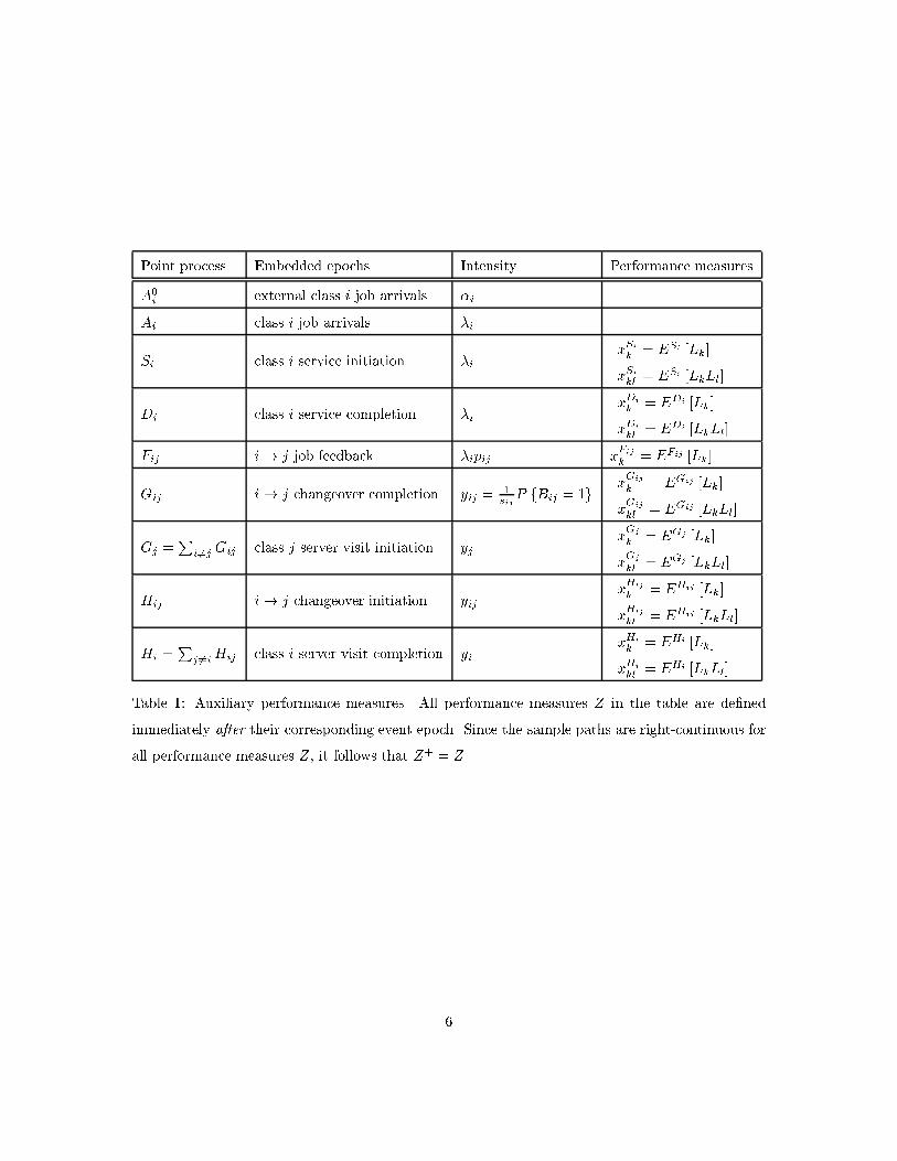
We consider three types of auxiliary performance measures: The �rst type represents Palm mo-

ments of queue lengths with respect to the point processes de�ned by certain embedded epochs. The

second type represents server's visit and changeover frequencies. We present these point processes

and auxiliary performance measures in Table 1.

In addition to those presented in Table 1, we consider a third type of auxiliary performance

measures representing moments of queue lengths at an arbitrary time:

� xij = E [Lj j Bi = 1] (mean number of j-jobs in the system at an arbitrary time during the

service of i-jobs); X = (xij )i;j2N ;

� x0j = E [Lj j B = 0] (mean number of j-jobs in the system at an arbitrary time while the server

is idle); x0 = (x0j )j2N .

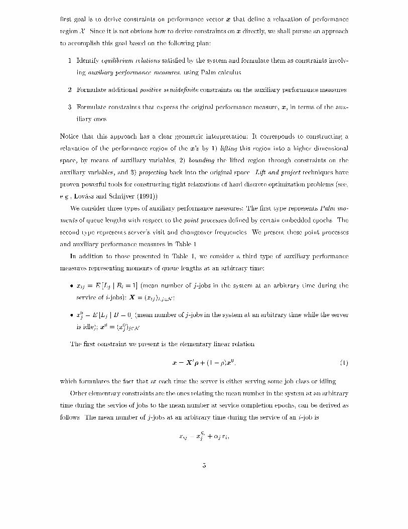
The �rst constraint we present is the elementary linear relation

x =X0�+ (1� �)x0; (1)

which formulates the fact that at each time the server is either serving some job class or idling.

Other elementary constraints are the ones relating the mean number in the system at an arbitrary

time during the service of jobs to the mean number at service completion epochs, can be derived as

follows. The mean number of j-jobs at an arbitrary time during the service of an i-job is

xij = xSij + �j ri;

5

Point process Embedded epochs Intensity Performance measures

A0i external class i job arrivals �i

Ai class i job arrivals �i

Si class i service initiation �ixSik = ESi [Lk]

xSikl = ESi [LkLl]

Di class i service completion �ixDi

k = EDi [Lk]

xDi

kl = EDi [LkLl]

Fij i! j job feedback �ipij xFijk = EFij [Lk]

Gij i! j changeover completion yij =1sijP fBij = 1g

xGij

k = EGij [Lk]

xGij

kl = EGij [LkLl]

Gj =P

i6=j Gij class j server visit initiation yjxGj

k = EGj [Lk]

xGj

kl = EGj [LkLl]

Hij i! j changeover initiation yijxHij

k = EHij [Lk]

xHij

kl = EHij [LkLl]

Hi =P

j 6=iHij class i server visit completion yixHi

k = EHi [Lk]

xHi

kl = EHi [LkLl]

Table 1: Auxiliary performance measures. All performance measures Z in the table are de�ned

immediately after their corresponding event epoch. Since the sample paths are right-continuous for

all performance measures Z, it follows that Z+ = Z.

6

i.e., the number of j-jobs at the beginning of an i-service plus the mean number of external class j

arrivals until an arbitrary time during an i-service. Furthermore, we have

xDi

j = xSij + �i�j + pij � �ij ; (2)

where �ij is Kronecker's delta function. Subtracting the previous equations, we obtain

xij = xDi

j + (ri � �i)�j + �ij � pij : (3)

In matrix notation,

X =XD + (r � �)�0 + I �P ; (4)

where XD =�xDi

j

�i;j2N

.

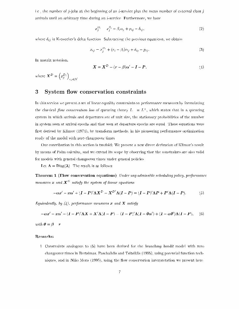
3 System ow conservation constraints

In this section we present a set of linear equality constraints on performance measures by formulating

the classical ow conservation law of queueing theory L� = L+, which states that in a queueing

system in which arrivals and departures are of unit size, the stationary probabilities of the number

in system seen at arrival epochs and that seen at departure epochs are equal. These equations were

�rst derived by Klimov (1974), by transform methods, in his pioneering performance optimization

study of the model with zero changeover times.

Our contribution in this section is twofold: We present a new direct derivation of Klimov's result

by means of Palm calculus, and we extend its scope by observing that the constraints are also valid

for models with general changeover times under general policies.

Let � = Diag(�). The result is as follows:

Theorem 1 (Flow conservation equations) Under any admissible scheduling policy, performance

measures x and XD satisfy the system of linear equations

��x0 � x�0 + (I �P )0�XD +XD 0�(I �P ) = (I �P )0�P +P

0�(I �P ): (5)

Equivalently, by (4), performance measures x and X satisfy

��x0 � x�0 + (I �P )0�X +X0�(I �P ) = (I �P )0�(I � ��0) + (I ���0)�(I �P ); (6)

with � = � � r.

Remarks:

1. Constraints analogous to (5) have been derived for the branching bandit model with zero

changeover times in Bertsimas, Paschalidis and Tsitsiklis (1995), using potential function tech-

niques, and in Ni~no-Mora (1995), using the ow conservation interpretation we present here.

7

They further show that the region in x-space de�ned by constraints analogous to (1), (4), (5),

together with x0 = 0 and x � 0, is the exact performance region of the x's. It is noteworthy

that the ow conservation law L� = L+ leads to a compact reformulation (having polynomial

size on the number of job classes) of the x's performance region, that involves the matrix of

auxiliary variables X, whereas the exact formulation on the original variables x was found to

have exponential size in Bertsimas and Ni~no-Mora (1996).

2. Notice that constraints (5) do not involve changeover time parameters. This is because they

are valid under any admissible scheduling policy, regardless of whether it is work-conserving.

3. An interesting consequence of constraints (5) is the following: They imply, together with

relations (1) and (4), that the vector of expected queue lengths at an arbitrary time, x,

as well as the vector of expected queue lengths at an arbitrary server idling time, x0, are

uniquely determined by the matrix of expected queue lengths at service completion epochs,

XD. Therefore, in order to formulate the performance region of the x's we need only to focus

on formulating constraints on matrix XD.

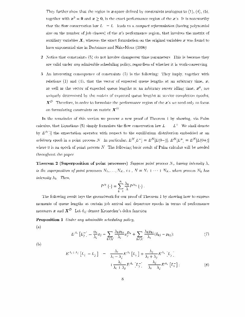
In the remainder of this section we present a new proof of Theorem 1 by showing, via Palm

calculus, that Equations (5) simply formulate the ow conservation law L� = L+. We shall denote

by EN [�] the expectation operator with respect to the equilibrium distribution embedded at an

arbitrary epoch in a point process N . In particular, EN [L�] = EN [L(0�)], EN [L+] = EN [L(0+)]

where 0 is an epoch of point process N . The following basic result of Palm calculus will be needed

throughout the paper.

Theorem 2 (Superposition of point processes) Suppose point process N , having intensity �,

is the superposition of point processes N1; : : : ; NK , i.e., N = N1 + � � �+NK , where process Nk has

intensity �k. Then,

PN f�g =

KXk=1

�k

�PNk f�g :

The following result lays the groundwork for our proof of Theorem 1 by showing how to express

moments of queue lengths at certain job arrival and departure epochs in terms of performance

measures x and XD. Let �ij denote Kronecker's delta function.

Proposition 1 Under any admissible scheduling policy,

(a)

EAi

�L�j�=

�i

�ixj +

Xk2N

�kpki

�ixDk

j +Xk2N

�kpki

�i(�kj � pkj); (7)

(b)

EAi+Aj

�L�i + L�j

�=

�i

�i + �jEAi

�L�i�+

�j

�i + �jEAj

�L�j�

+�i

�i + �jEAi

�L�j�+

�j

�i + �jEAj

�L�i�; (8)

8

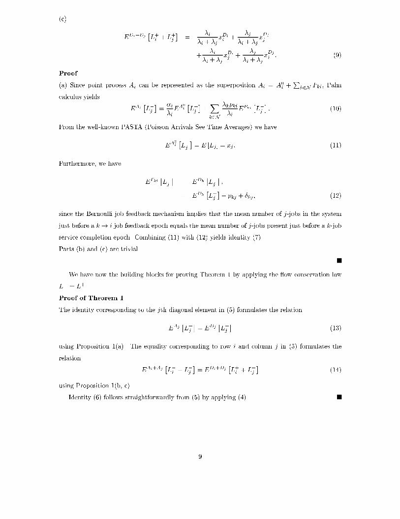
(c)

EDi+Dj

�L+i + L+

j

�=

�i

�i + �jxDi

i +�j

�i + �jxDj

j

+�i

�i + �jxDi

j +�j

�i + �jxDj

i : (9)

Proof

(a) Since point process Ai can be represented as the superposition Ai = A0i +

Pk2N Fki, Palm

calculus yields

EAi

�L�j�=

�i

�iEA0

i

�L�j�+Xk2N

�kpki

�iEFki

�L�j�: (10)

From the well-known PASTA (Poisson Arrivals See Time Averages) we have

EA0

i

�L�j�= E [Lj ] = xj : (11)

Furthermore, we have

EFki�L�j�

= EDk

�L�j�;

= EDk

�L+j

�� pkj + �kj ; (12)

since the Bernoulli job feedback mechanism implies that the mean number of j-jobs in the system

just before a k ! i job feedback epoch equals the mean number of j-jobs present just before a k-job

service completion epoch. Combining (11) with (12) yields identity (7).

Parts (b) and (c) are trivial.

We have now the building blocks for proving Theorem 1 by applying the ow conservation law

L� = L+.

Proof of Theorem 1.

The identity corresponding to the jth diagonal element in (5) formulates the relation

EAj

�L�j�= EDj

�L+j

�(13)

using Proposition 1(a). The equality corresponding to row i and column j in (5) formulates the

relation

EAi+Aj

�L�i + L�j

�= EDi+Dj

�L+i + L+

j

�(14)

using Proposition 1(b, c).

Identity (6) follows straightforwardly from (5) by applying (4).

9

Remarks.

1. Notice that identities (13) and (14) formulate the ow conservation law L� = L+ as applied

to the queues of j-jobs and fi; jg-jobs considered in isolation, for all pairs fi; jg of job classes.

2. It is interesting to observe that we do not obtain additional constraints by formulating the

ow conservation law

EP

i2SAi

"Xi2S

L�i

#= E

Pi2S

Di

"Xi2S

L+i

#

for subsets of job classes S of size larger than 3. The equations for jSj � 3 turn out to be

implied by those for jSj � 2.

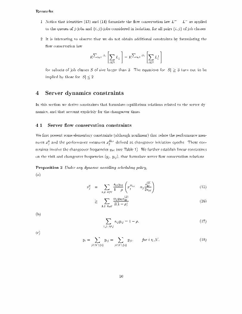
4 Server dynamics constraints

In this section we derive constraints that formulate equilibrium relations related to the server dy-

namics, and that account explicitly for the changeover times.

4.1 Server ow conservation constraints

We �rst present some elementary constraints (although nonlinear) that relate the performance mea-

sures x0j and the performance measures xHkl

j de�ned at changeover initiation epochs. These con-

straints involve the changeover frequencies ykl (see Table 1). We further establish linear constraints

on the visit and changeover frequencies (yj , yij), that formulate server ow conservation relations.

Proposition 2 Under any dynamic nonidling scheduling policy,

(a)

x0j =X

k;l: k 6=l

sklykl

1� �

xHkl

j + �js(2)kl

2skl

!(15)

�X

k;l: k 6=l

�jykls(2)kl

2(1� �)(16)

(b) Xi;j: i6=j

sijyij = 1� �: (17)

(c)

yi =X

j2Nnfig

yij =X

j2Nnfig

yji; for i 2 N : (18)

10

Proof

(a) Eq. (15) follows from the elementary relations (valid under nonidling policies)

x0j =X

k;l: k 6=l

sklykl

1� �E [Lj j Bkl = 1]

=X

k;l: k 6=l

sklykl

1� �

xHkl

j + �js(2)kl

2skl

!:

Inequality (16) follows directly from Eq. (15):

x0j =X

k;l: k 6=l

sklykl

1� �E [Lj j Bkl = 1]

�X

k;l: k 6=l

sklykl

1� ��j

s(2)kl

2skl:

(b) Eq. (17) formulates the requirements that policies must be nonidling, using the fact that

P fBij = 1g = sijyij .

(c) Eq. (18) formulates a simple ow conservation relation: the rates at which the server visits and

leaves the i-queue are equal.

4.2 Server visit constraints

We derive in this section a family of nonlinear constraints by formulating a key relation between the

point processes de�ned in Table 1. In the notation of Palm calculus, this relation is written as

Gi +Di = Hi + Si; for i 2 N ; (19)

and it expresses the elementary fact that, under any nonidling policy, each time a visit initiation

or a service completion occurs, coincidentally there also occurs either a service beginning or a visit

completion. Identity (19) was �rst observed by Eisenberg (1972), who applied it as a central tool in

his pioneering analysis (via transform methods) of polling systems with changeover times.

We show next that identity (19) allows us to represent Palm moments at service completion

epochs (xDi

j ) in terms of Palm moments at visit initiation and completion epochs (xGi

k , xGi

kl , xHi

k ,

xHi

kl ; see Table 1), and to formulate additional constraints between the two latter kinds of moments.

We state and prove next our main result.

Theorem 3 Under any dynamic nonidling policy,

(a)

yi

�xHi

j � xGi

j

�= �i(�j�i + pij � �ij) for i; j 2 N : (20)

(b)

yi

�xHi

jk � xGi

jk

�= �i

���k�i + pik � �ik

�xDi

j +

��j�i + pij � �ij

�xDi

k

11

�

��j(pik � �ik) + �k(pij � �ij) + �j�kj

��i + �j�k

��(2)i � 2�2i

�

pij�ik + pik�ij + pij�kj � �ij�ik � 2pikpij

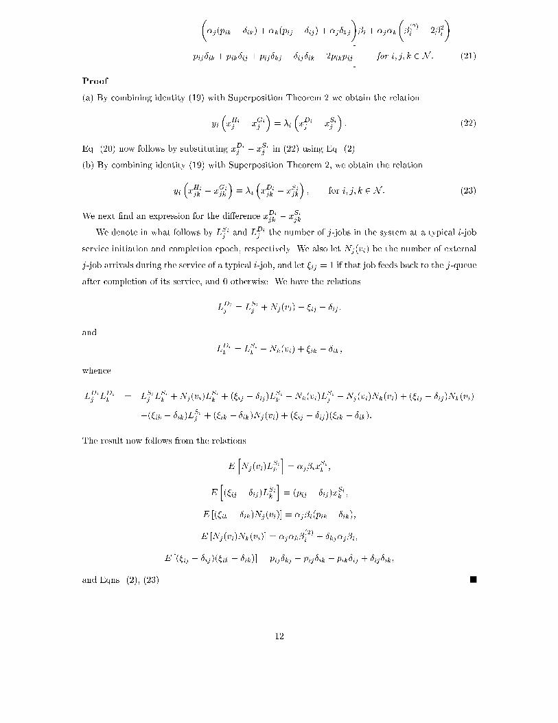
�for i; j; k 2 N : (21)

Proof

(a) By combining identity (19) with Superposition Theorem 2 we obtain the relation

yi

�xHi

j � xGi

j

�= �i

�xDi

j � xSij

�: (22)

Eq. (20) now follows by substituting xDi

j � xSij in (22) using Eq. (2).

(b) By combining identity (19) with Superposition Theorem 2, we obtain the relation

yi

�xHi

jk � xGi

jk

�= �i

�xDi

jk � xSijk

�; for i; j; k 2 N : (23)

We next �nd an expression for the di�erence xDi

jk � xSijk .

We denote in what follows by LSij and LDi

j the number of j-jobs in the system at a typical i-job

service initiation and completion epoch, respectively. We also let Nj(vi) be the number of external

j-job arrivals during the service of a typical i-job, and let �ij = 1 if that job feeds back to the j-queue

after completion of its service, and 0 otherwise. We have the relations

LDi

j = LSij +Nj(vi) + �ij � �ij ;

and

LDi

k = LSik +Nk(vi) + �ik � �ik;

whence

LDi

j LDi

k = LSij LSik +Nj(vi)LSik + (�ij � �ij)L

Sik +Nk(vi)L

Sij +Nj(vi)Nk(vi) + (�ij � �ij)Nk(vi)

+(�ik � �ik)LSij + (�ik � �ik)Nj(vi) + (�ij � �ij)(�ik � �ik):

The result now follows from the relations

EhNj(vi)L

Sik

i= �j�ix

Sik ;

Eh(�ij � �ij)L

Sik

i= (pij � �ij)x

Sik ;

E [(�ik � �ik)Nj(vi)] = �j�i(pik � �ik);

E [Nj(vi)Nk(vi)] = �j�k�(2)i + �kj�j�i;

E [(�ij � �ij)(�ik � �ik)] = pij�kj � pij�ik � pik�ij + �ij�ik;

and Eqns. (2), (23).

12

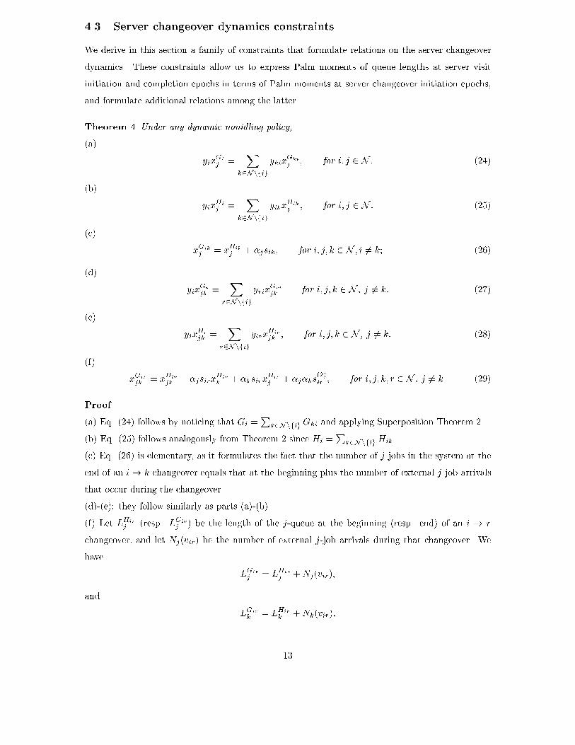
4.3 Server changeover dynamics constraints

We derive in this section a family of constraints that formulate relations on the server changeover

dynamics. These constraints allow us to express Palm moments of queue lengths at server visit

initiation and completion epochs in terms of Palm moments at server changeover initiation epochs,

and formulate additional relations among the latter.

Theorem 4 Under any dynamic nonidling policy,

(a)

yixGi

j =X

k2Nnfig

ykixGki

j ; for i; j 2 N : (24)

(b)

yixHi

j =X

k2Nnfig

yikxHik

j ; for i; j 2 N : (25)

(c)

xGik

j = xHik

j + �jsik; for i; j; k 2 N ; i 6= k; (26)

(d)

yixGi

jk =X

r2Nnfig

yrixGri

jk for i; j; k 2 N , j 6= k: (27)

(e)

yixHi

jk =X

r2Nnfig

yirxHir

jk ; for i; j; k 2 N , j 6= k: (28)

(f)

xGir

jk = xHir

jk + �jsirxHir

k + �ksirxHir

j + �j�ks(2)ir ; for i; j; k; r 2 N , j 6= k. (29)

Proof

(a) Eq. (24) follows by noticing that Gi =P

k2NnfigGki and applying Superposition Theorem 2.

(b) Eq. (25) follows analogously from Theorem 2 since Hi =P

k2NnfigHik .

(c) Eq. (26) is elementary, as it formulates the fact that the number of j-jobs in the system at the

end of an i! k changeover equals that at the beginning plus the number of external j-job arrivals

that occur during the changeover.

(d)-(e): they follow similarly as parts (a)-(b).

(f) Let LHir

j (resp. LGir

j ) be the length of the j-queue at the beginning (resp. end) of an i ! r

changeover, and let Nj(vir) be the number of external j-job arrivals during that changeover. We

have

LGir

j = LHir

j +Nj(vir);

and

LGir

k = LHir

k +Nk(vir);

13

whence

LGir

j LGir

k = LHir

j LHir

k +Nj(vir)LHir

k +Nk(vir)LHir

j +Nj(vir)Nk(vir):

Now, since

EhNj(vir)L

Hir

k

i= �jsirx

Hir

k

and

E [Nk(vir)Nj(vir)] = �k�js(2)ir ;

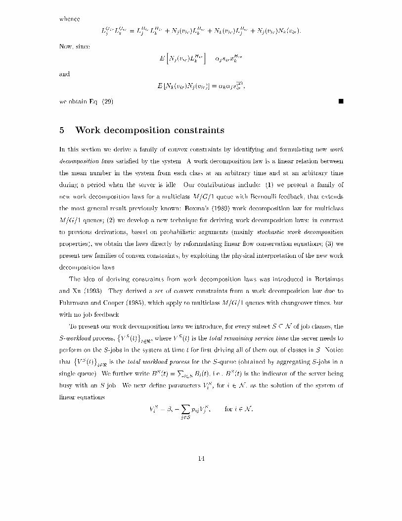
we obtain Eq. (29).

5 Work decomposition constraints

In this section we derive a family of convex constraints by identifying and formulating new work

decomposition laws satis�ed by the system. A work decomposition law is a linear relation between

the mean number in the system from each class at an arbitrary time and at an arbitrary time

during a period when the server is idle. Our contributions include: (1) we present a family of

new work decomposition laws for a multiclass M=G=1 queue with Bernoulli feedback, that extends

the most general result previously known: Boxma's (1989) work decomposition law for multiclass

M=G=1 queues; (2) we develop a new technique for deriving work decomposition laws: in contrast

to previous derivations, based on probabilistic arguments (mainly stochastic work decomposition

properties), we obtain the laws directly by reformulating linear ow conservation equations; (3) we

present new families of convex constraints, by exploiting the physical interpretation of the new work

decomposition laws.

The idea of deriving constraints from work decomposition laws was introduced in Bertsimas

and Xu (1993). They derived a set of convex constraints from a work decomposition law due to

Fuhrmann and Cooper (1985), which apply to multiclassM=G=1 queues with changeover times, but

with no job feedback.

To present our work decomposition laws we introduce, for every subset S � N of job classes, the

S-workload process,�V S(t)

t2<

, where V S(t) is the total remaining service time the server needs to

perform on the S-jobs in the system at time t for �rst driving all of them out of classes in S. Notice

that�V S(t)

t2<

is the total workload process for the S-queue (obtained by aggregating S-jobs in a

single queue). We further write BS(t) =P

i2S Bi(t), i.e., BS(t) is the indicator of the server being

busy with an S-job. We next de�ne parameters V Si , for i 2 N , as the solution of the system of

linear equations

V Si = �i +

Xj2S

pijVSj ; for i 2 N :

14

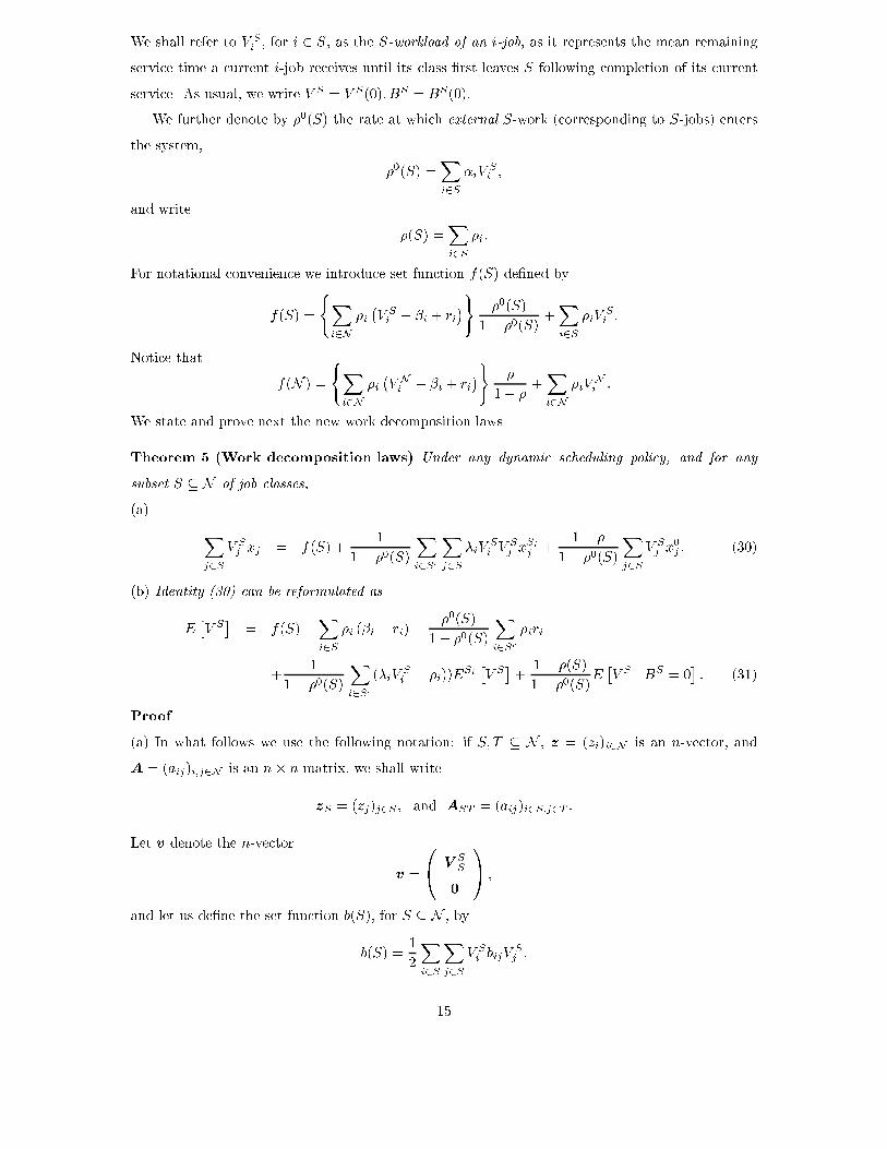
We shall refer to V Si , for i 2 S, as the S-workload of an i-job, as it represents the mean remaining

service time a current i-job receives until its class �rst leaves S following completion of its current

service. As usual, we write V S = V S(0); BS = BS(0):

We further denote by �0(S) the rate at which external S-work (corresponding to S-jobs) enters

the system,

�0(S) =Xi2S

�iVSi ;

and write

�(S) =Xi2S

�i:

For notational convenience we introduce set function f(S) de�ned by

f(S) =

(Xi2N

�i�V Si � �i + ri

�) �0(S)

1� �0(S)+Xi2S

�iVSi :

Notice that

f(N ) =

(Xi2N

�i�V Ni � �i + ri

�) �

1� �+Xi2N

�iVNi :

We state and prove next the new work decomposition laws.

Theorem 5 (Work decomposition laws) Under any dynamic scheduling policy, and for any

subset S � N of job classes,

(a)

Xj2S

V Sj xj = f(S) +

1

1� �0(S)

Xi2Sc

Xj2S

�iVSi V

Sj x

Sij +

1� �

1� �0(S)

Xj2S

V Sj x

0j : (30)

(b) Identity (30) can be reformulated as

E�V S�

= f(S)�Xi2S

�i (�i � ri)��0(S)

1� �0(S)

Xi2Sc

�iri

+1

1� �0(S)

Xi2Sc

(�iVSi � �i))E

Si�V S�+

1� �(S)

1� �0(S)E�V S j BS = 0

�: (31)

Proof

(a) In what follows we use the following notation: if S; T � N , z = (zi)i2N is an n-vector, and

A = (aij)i;j2N is an n� n matrix, we shall write

zS = (zj)j2S ; and AST = (aij)i2S;j2T :

Let v denote the n-vector

v =

0@ V

SS

0

1A ;

and let us de�ne the set function b(S), for S � N , by

b(S) =1

2

Xi2S

Xj2S

V Si bijV

Sj ;

15

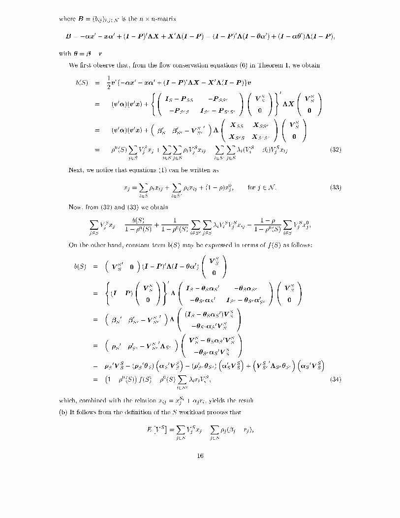
where B = (bij)i;j2N is the n� n-matrix

B = ��x0 � x�0 + (I �P )0�X +X0�(I �P ) = (I �P )0�(I � ��0) + (I ���0)�(I �P );

with � = � � r.

We �rst observe that, from the ow conservation equations (6) in Theorem 1, we obtain

b(S) =1

2v0f��x0 � x�0 + (I �P )0�X +X

0�(I �P )gv

= �(v0�)(v0x) +

8<:0@ IS �P SS �P SSc

�P ScS ISc �P ScSc

1A0@ V

SS

0

1A9=;0

�X

0@ V

SS

0

1A

= �(v0�)(v0x) +��0S �

0Sc � V

SSc0��

0@ XSS XSSc

XScS XScSc

1A0@ V

SS

0

1A

= ��0(S)Xj2S

V Sj xj +

Xi2S

Xj2S

�iVSj xij �

Xi2Sc

Xj2S

�i(VSi � �i)V

Sj xij (32)

Next, we notice that equations (1) can be written as

xj =Xi2S

�ixij +Xi2Sc

�ixij + (1� �)x0j ; for j 2 N : (33)

Now, from (32) and (33) we obtain

Xj2S

V Sj xj =

b(S)

1� �0(S)+

1

1� �0(S)

Xi2Sc

Xj2S

�iVSi V

Sj xij +

1� �

1� �0(S)

Xi2S

V Sj x

0j ;

On the other hand, constant term b(S) may be expressed in terms of f(S) as follows:

b(S) =�V

SS

00

�(I �P )0�(I � ��0)

0@ V

SS

0

1A

=

8<:(I �P )

0@ V

SS

0

1A9=;0

�

0@ IS � �S�S

0 ��S�Sc

��Sc�S0

ISc � �Sc�0Sc

1A0@ V

SS

0

1A

=��S

0�0Sc � V

SSc0��

0@ (IS � �S�S

0)V SS

��Sc�S0V

SS

1A

=��S

0�0Sc � V

SSc0�Sc

�0@ VSS � �S�S

0V

SS

��Sc�S0V

SS

1A

= �S0V

SS � (�S

0�S)

��S

0V

SS

�� (�0Sc�Sc)

��0SV

SS

�+�V

SSc0�Sc�Sc

���S

0V

SS

�=

�1� �0(S)

�f(S)� �0(S)

Xi2Sc

�iriVSi ; (34)

which, combined with the relation xij = xSij + �jri, yields the result.

(b) It follows from the de�nition of the S-workload process that

E�V S�=Xj2S

V Sj xj �

Xj2S

�j(�j � rj);

16

ESi�V S�=Xj2S

V Sj x

Sij ;

and

E�V S j B = 0

�=Xj2S

V Sj x

0j ;

which, combined with (30), yields

E�V S�= f(S)�

Xi2S

�i (�i � ri) +1

1� �0(S)

Xi2Sc

�iVSi E

Si�V S�+

1� �

1� �0(S)E�V S j B = 0

�: (35)

Eq. (31) follows from Eq. (35) by substituting E�V S j B = 0

�using the elementary relations

E�V S j BS = 0

�=

�(Sc)

1� �(S)EhV S j BSc = 1

i+

1� �

1� �(S)E�V S j B = 0

�; (36)

and

�(Sc)EhV S j BSc = 1

i=Xi2Sc

�i�ESi

�V S�+ �0(S)ri

�: (37)

Remarks:

1. Notice that for S = N Theorem 5 yields the work decomposition law

Xi2N

V Ni xi = f(N ) +

Xi2N

V Ni x0i ; (38)

which was �rst derived by Boxma (1989) by a stochastic work decomposition argument. It

means that the total mean workload (i.e, the total amount of service needed to clear the system

of all jobs currently present) decomposes into two terms: a) the total mean workload in the

corresponding work-conserving system, f(N ), and b) the total mean workload at an arbitrary

time when the server is idle.

2. For S � N the work decomposition laws in Theorem 5 are new, as they do not follow from

Boxma's (1989) stochastic work decomposition theorem. The assumption in Boxma's theorem

that is violated here is that arrivals during idle periods for the S-queue are not Poisson, as

they include jobs fed back from the Sc-queue.

3. From Theorem 5 we obtain the linear workload bound on S-jobs

Xi2S

V Si xi � f(S); (39)

valid under all dynamic policies. In addition, for systems with zero changeover times inequality

(39) is satis�ed at equality under any dynamic nonidling policy that gives nonpreemptive

priority to S-jobs over Sc-jobs. The reason is that under such policies xSij = 0 for i 2 Sc and

17

j 2 S, and x0 = 0. In particular, inequality (39) holds with equality when S = N . Therefore,

for the special case of zero changeover times performance vector x satis�es the generalized work

conservation laws introduced by Bertsimas and Ni~no-Mora (1996), and thus the performance

region spanned by the x's under dynamic nonidling policies is the polyhedron de�ned by the

family of inequalities (39), for S � N , together with the equationP

i2N V Ni xi = f(N ).

Tsoucas (1991) �rst identi�ed the structure of workload bounds (39), but did not evaluate the

f(S) function. These workload bounds generalize those discovered by Gelenbe and Mitrani

(1980) for multiclass M=GI=1 queues without job feedback.

5.1 Strengthened workload bounds from work decomposition laws

In this section we apply the work decomposition laws in Theorem 5 to develop two new families of

workload bounds, which strengthen bound (39) by incorporating the e�ect of positive changeover

times.

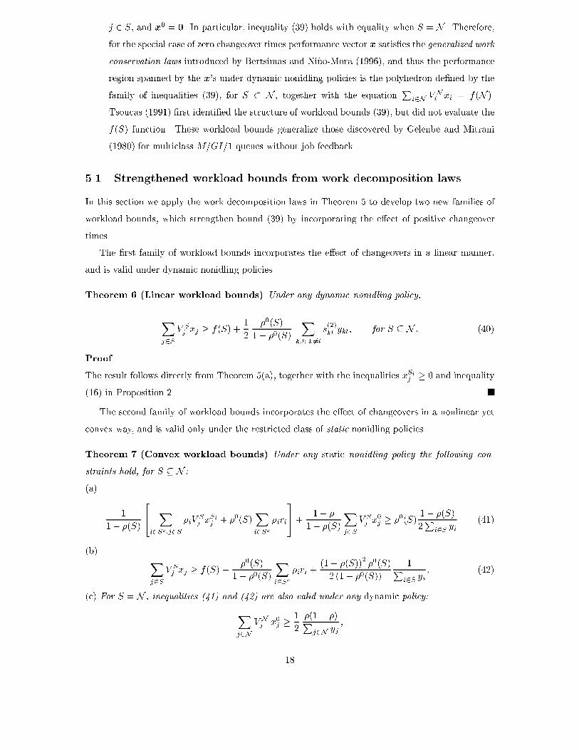
The �rst family of workload bounds incorporates the e�ect of changeovers in a linear manner,

and is valid under dynamic nonidling policies.

Theorem 6 (Linear workload bounds) Under any dynamic nonidling policy,

Xj2S

V Sj xj � f(S) +

1

2

�0(S)

1� �0(S)

Xk;l: k 6=l

s(2)kl ykl; for S � N : (40)

Proof

The result follows directly from Theorem 5(a), together with the inequalities xSij � 0 and inequality

(16) in Proposition 2.

The second family of workload bounds incorporates the e�ect of changeovers in a nonlinear yet

convex way, and is valid only under the restricted class of static nonidling policies.

Theorem 7 (Convex workload bounds) Under any static nonidling policy the following con-

straints hold, for S � N :

(a)

1

1� �(S)

24 Xi2Sc;j2S

�iVSj x

Sij + �0(S)

Xi2Sc

�iri

35+

1� �

1� �(S)

Xj2S

V Sj x

0j � �0(S)

1� �(S)

2P

i2S yi(41)

(b) Xj2S

V Sj xj � f(S)�

�0(S)

1� �0(S)

Xi2Sc

�iri +(1� �(S))

2�0(S)

2 (1� �0(S))

1Pi2S yi

: (42)

(c) For S = N , inequalities (41) and (42) are also valid under any dynamic policy:

Xj2N

V Nj x0j �

1

2

�(1� �)Pj2N yj

;

18

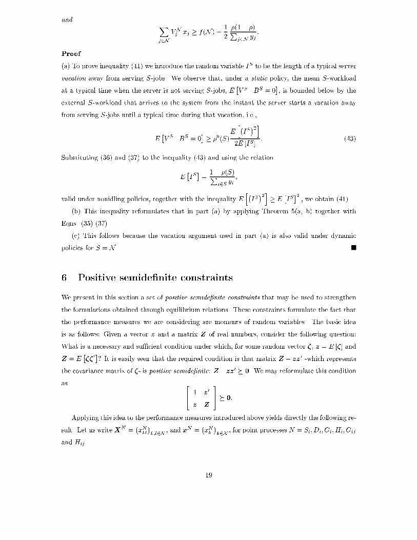
and Xj2N

V Nj xj � f(N ) +

1

2

�(1� �)Pj2N yj

:

Proof

(a) To prove inequality (41) we introduce the random variable IS to be the length of a typical server

vacation away from serving S-jobs. We observe that, under a static policy, the mean S-workload

at a typical time when the server is not serving S-jobs, E�V S j BS = 0

�, is bounded below by the

external S-workload that arrives to the system from the instant the server starts a vacation away

from serving S-jobs until a typical time during that vacation, i.e.,

E�V S j BS = 0

�� �0(S)

Eh�IS�2i

2E [IS ]: (43)

Substituting (36) and (37) to the inequality (43) and using the relation

E�IS�=

1� �(S)Pi2S yi

;

valid under nonidling policies, together with the inequality Eh�IS�2i

� E�IS�2; we obtain (41).

(b) This inequality reformulates that in part (a) by applying Theorem 5(a, b) together with

Eqns. (35)-(37).

(c) This follows because the vacation argument used in part (a) is also valid under dynamic

policies for S = N .

6 Positive semide�nite constraints

We present in this section a set of positive semide�nite constraints that may be used to strengthen

the formulations obtained through equilibrium relations. These constraints formulate the fact that

the performance measures we are considering are moments of random variables. The basic idea

is as follows: Given a vector z and a matrix Z of real numbers, consider the following question:

What is a necessary and su�cient condition under which, for some random vector �, z = E [�] and

Z = E���

0�? It is easily seen that the required condition is that matrix Z � zz0 -which represents

the covariance matrix of �- is positive semide�nite: Z�zz0 � 0. We may reformulate this condition

as 24 1 z

0

z Z

35 � 0:

Applying this idea to the performance measures introduced above yields directly the following re-

sult. Let us writeXN =�xNkl�k;l2N

, and xN =�xNk�k2N

, for point processes N = Si; Di; Gi; Hi; Gij

and Hij .

19

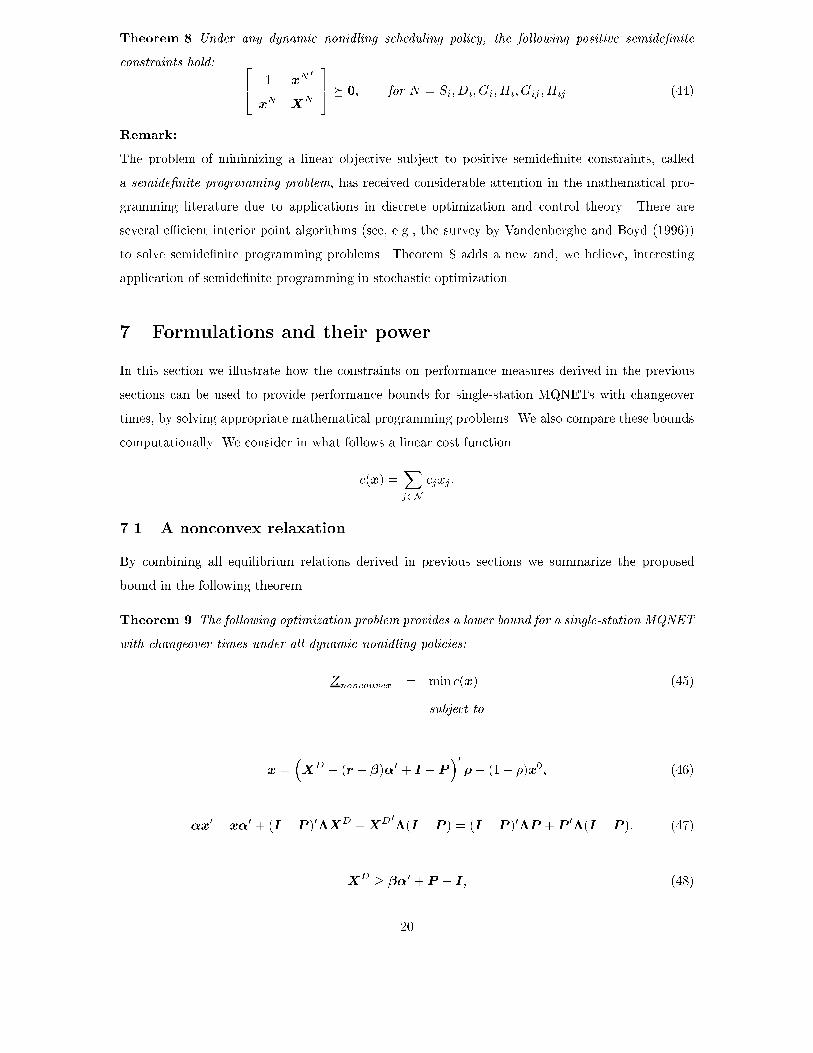
Theorem 8 Under any dynamic nonidling scheduling policy, the following positive semide�nite

constraints hold: 24 1 x

N 0

xN

XN

35 � 0; for N = Si; Di; Gi; Hi; Gij ; Hij . (44)

Remark:

The problem of minimizing a linear objective subject to positive semide�nite constraints, called

a semide�nite programming problem, has received considerable attention in the mathematical pro-

gramming literature due to applications in discrete optimization and control theory. There are

several e�cient interior point algorithms (see, e.g., the survey by Vandenberghe and Boyd (1996))

to solve semide�nite programming problems. Theorem 8 adds a new and, we believe, interesting

application of semide�nite programming in stochastic optimization.

7 Formulations and their power

In this section we illustrate how the constraints on performance measures derived in the previous

sections can be used to provide performance bounds for single-station MQNETs with changeover

times, by solving appropriate mathematical programming problems. We also compare these bounds

computationally. We consider in what follows a linear cost function

c(x) =Xj2N

cjxj :

7.1 A nonconvex relaxation

By combining all equilibrium relations derived in previous sections we summarize the proposed

bound in the following theorem.

Theorem 9 The following optimization problem provides a lower bound for a single-station MQNET

with changeover times under all dynamic nonidling policies:

Znonconvex = min c(x) (45)

subject to

x =�X

D + (r � �)�0 + I �P�0�+ (1� �)x0; (46)

��x0 � x�0 + (I �P )0�XD +XD 0�(I �P ) = (I �P )0�P +P

0�(I �P ): (47)

XD � ��

0 +P � I ; (48)

20

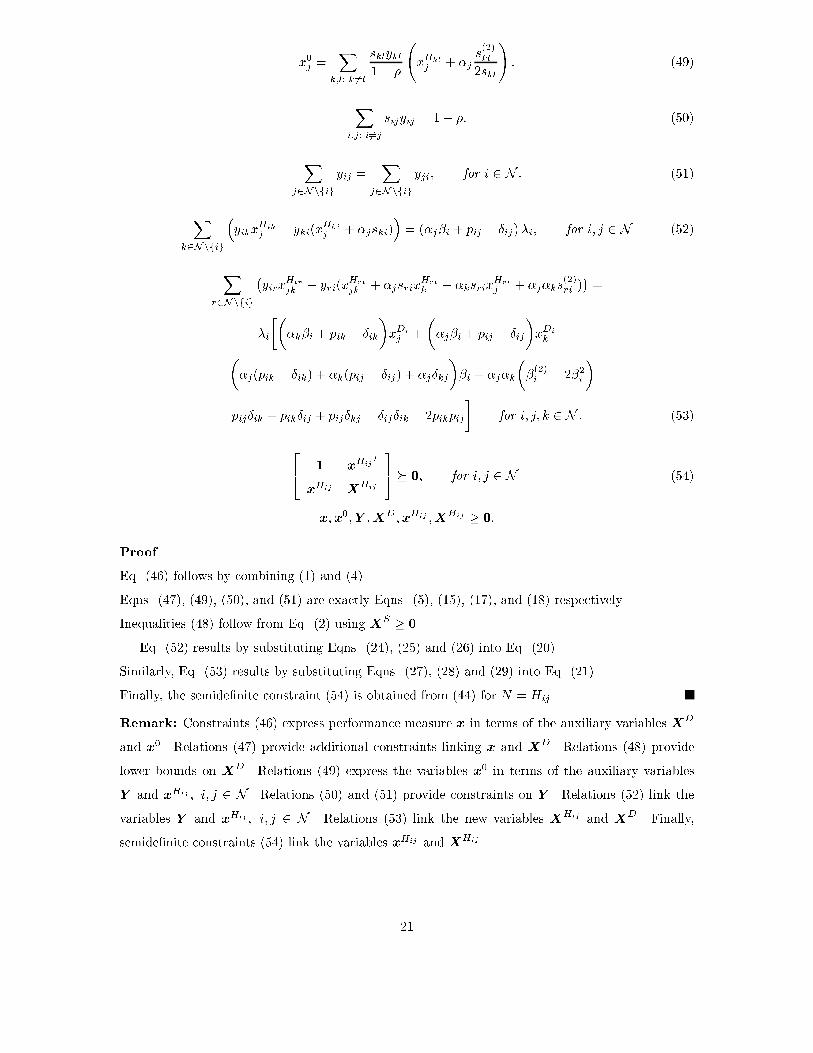
x0j =X

k;l: k 6=l

sklykl

1� �

xHkl

j + �js(2)kl

2skl

!: (49)

Xi;j: i6=j

sijyij = 1� �: (50)

Xj2Nnfig

yij =X

j2Nnfig

yji; for i 2 N : (51)

Xk2Nnfig

�yikx

Hik

j � yki(xHki

j + �jski)�= (�j�i + pij � �ij)�i; for i; j 2 N (52)

Xr2Nnfig

�yirx

Hir

jk � yri(xHri

jk + �jsrixHri

k + �ksrixHri

j + �j�ks(2)ri )�=

�i

���k�i + pik � �ik

�xDi

j +

��j�i + pij � �ij

�xDi

k

�

��j(pik � �ik) + �k(pij � �ij) + �j�kj

��i + �j�k

��(2)i � 2�2i

�

pij�ik + pik�ij + pij�kj � �ij�ik � 2pikpij

�for i; j; k 2 N : (53)

24 1 x

Hij0

xHij X

Hij

35 � 0; for i; j 2 N . (54)

x;x0;Y ;XD ;xHij ;XHij � 0:

Proof

Eq. (46) follows by combining (1) and (4).

Eqns. (47), (49), (50), and (51) are exactly Eqns. (5), (15), (17), and (18) respectively.

Inequalities (48) follow from Eq. (2) using XS � 0.

Eq. (52) results by substituting Eqns. (24), (25) and (26) into Eq. (20).

Similarly, Eq. (53) results by substituting Eqns. (27), (28) and (29) into Eq. (21).

Finally, the semide�nite constraint (54) is obtained from (44) for N = Hij .

Remark: Constraints (46) express performance measure x in terms of the auxiliary variables XD

and x0. Relations (47) provide additional constraints linking x and XD. Relations (48) provide

lower bounds on XD. Relations (49) express the variables x0 in terms of the auxiliary variables

Y and xHij ; i; j 2 N . Relations (50) and (51) provide constraints on Y . Relations (52) link the

variables Y and xHij ; i; j 2 N . Relations (53) link the new variables XHij and X

D. Finally,

semide�nite constraints (54) link the variables xHij and XHij .

21

On the solution of problem (45)

The optimization problem (45) is a nonlinear programming problem involving O(n4) variables. Un-

fortunately it is nonconvex due to the presence of the products ykixHki

j . However, if the values

of Y are known, the problem (in the remaining variables w = (x;XD;xHij ;XHij )) is a convex

semide�nite problem. Conversly, if the variables w are known, problem (45) is a linear optimization

problem. Given that there are very e�cient algorithms to solve linear and semide�nite optimization

problems, we can �x Y , solve for w, then given w solve for Y and so on. More formally we propose

the following algorithm:

Iterative Algorithm for solving (45)

1. Initialization. Start with a given Y 0; set w0 = 0; set k = 0; �x � > 0;

2. Semide�nite optimization problem. Let Y = Y 0; with Y �xed, solve the resulting

semide�nite optimization problem (45) for the variablesw; letw the resulting optimal solution;

set wk+1 = w;

3. Linear optimization problem. Letw = w; withw �xed, solve the resulting linear optimiza-

tion problem (45) for the variables Y . Let Y the resulting optimal solution; set Y k+1 = Y ;

4. Convergence test. If jjwk+1 �wkjj � � and jjY k+1 � Y kjj � �, stop; else set k:=k+1 and

go to step 2;

In Section 8 we illustrate that for speci�c classes of policies, like polling table and randomized

routing policies, we can calculate explicitly in terms of the original data the variables Y and y. As we

noticed earlier, problem (45) becomes a (convex) semide�nite optimization problem for which there

are very e�cient algorithms. As we discuss in Section 9, when solving problem (45), we calculate

the optimal values xHj

j of �rst order moments of queue lengths at visit completion epochs. These

values give rise to the following policy: If the server is currently serving j-jobs, terminate the current

visit when the queue length after a service completion does not exceed xHj

j , i.e., Lj � xHj

j . Notice

that if xHj

j = 0, then the server follows an exhaustive policy at the j-queue. In this way, given a

class of policies in which we can calculate the routing variables Y , we can �nd a threshold policy

for servicing jobs in the system by solving a convex semide�nite optimization problem.

7.2 Convex relaxations

In this section we propose several simpler but convex relaxations that can be used as an alternative

to problem (45).

Theorem 10 The following optimization problems provide lower bounds for a single-station MQNET

with changeover times under the classes os policies speci�ed:

22

(a) The linear optimization problem (under dynamic nonidling policies)

Zlinear = min c(x)

subject to (46); (47); (48); (50); (51); (16)

x;x0;XD;Y � 0;

involving O(n2) variables and constraints.

(b) The convex optimization problem (under static nonidling policies)

Zconvex1 = min c(x)

subject to (46); (47); (48); (50); (51); (16)

�(Sc)

1� �(S)

24 Xi2Sc;j2S

�iVSj (xDi

j � �i�j � pij) + �0(S)Xi2Sc

�iri

35

+1� �

1� �(S)

Xj2S

V Sj x

0j � �0(S)

1� �(S)

2P

i2S

Pj2Nnfig yij

S � N (55)

x;x0;XD;Y � 0;

involving O(n2) variables but an exponential number of convex constraints.

(c) The convex optimization problem (under static nonidling policies)

Zconvex2 = min c(x) (56)

subject to (40); (42); (17); (18)

x;Y ;y � 0;

involving also O(n2) variables but an exponential number of convex constraints.

Proof

(a) By maintaining only the linear constraints in the formulation (45) and using (16) instead of (49)

the bound Zlinear is obtained.

(b) The bound Zconvex1 is obtained from Zlinear by adding the family of convex constraints (41).

Notice that we used Eq. (2) to relate variables xSij and xDi

j . Moreover, we used the relation

yi =P

j2Nnfig yij (Eq. (18)).

(c) The bound Zconvex2 is immediate from Theorem 6.

Remark: In terms of their strength, the proposed relaxations can be ordered as follows:

Zlinear � Zconvex2 � Zconvex1 � Znonconvex;

i.e., there is a tradeo� between computational requirements and the strength of the bound.

23

� Zlinear Zconvex2 Zconvex1BestpriorityZconvex1

0.05 1.31 1.36 1.36 1.03

0.10 1.52 1.59 1.59 1.03

0.20 1.92 2.04 2.07 1.05

0.40 2.84 2.89 3.20 1.07

0.60 4.32 4.51 5.03 1.09

0.80 8.93 9.31 10.61 1.09

0.90 17.31 19.43 21.33 1.13

0.95 63.25 67.41 69.57 1.18

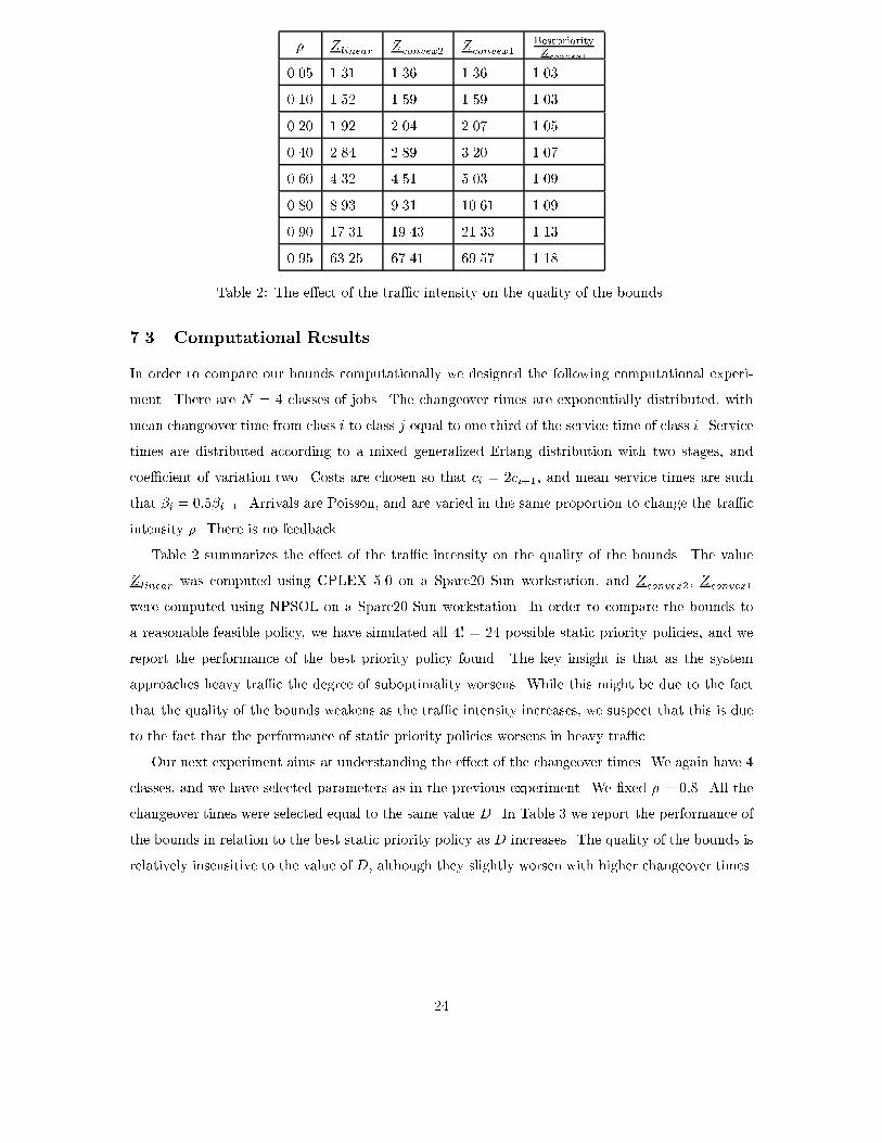
Table 2: The e�ect of the tra�c intensity on the quality of the bounds.

7.3 Computational Results

In order to compare our bounds computationally we designed the following computational experi-

ment. There are N = 4 classes of jobs. The changeover times are exponentially distributed, with

mean changeover time from class i to class j equal to one third of the service time of class i. Service

times are distributed according to a mixed generalized Erlang distribution with two stages, and

coe�cient of variation two. Costs are chosen so that ci = 2ci+1, and mean service times are such

that �i = 0:5�i+1. Arrivals are Poisson, and are varied in the same proportion to change the tra�c

intensity �. There is no feedback.

Table 2 summarizes the e�ect of the tra�c intensity on the quality of the bounds. The value

Zlinear was computed using CPLEX 5.0 on a Sparc20 Sun workstation, and Zconvex2; Zconvex1

were computed using NPSOL on a Sparc20 Sun workstation. In order to compare the bounds to

a reasonable feasible policy, we have simulated all 4! = 24 possible static priority policies, and we

report the performance of the best priority policy found. The key insight is that as the system

approaches heavy tra�c the degree of suboptimality worsens. While this might be due to the fact

that the quality of the bounds weakens as the tra�c intensity increases, we suspect that this is due

to the fact that the performance of static priority policies worsens in heavy tra�c.

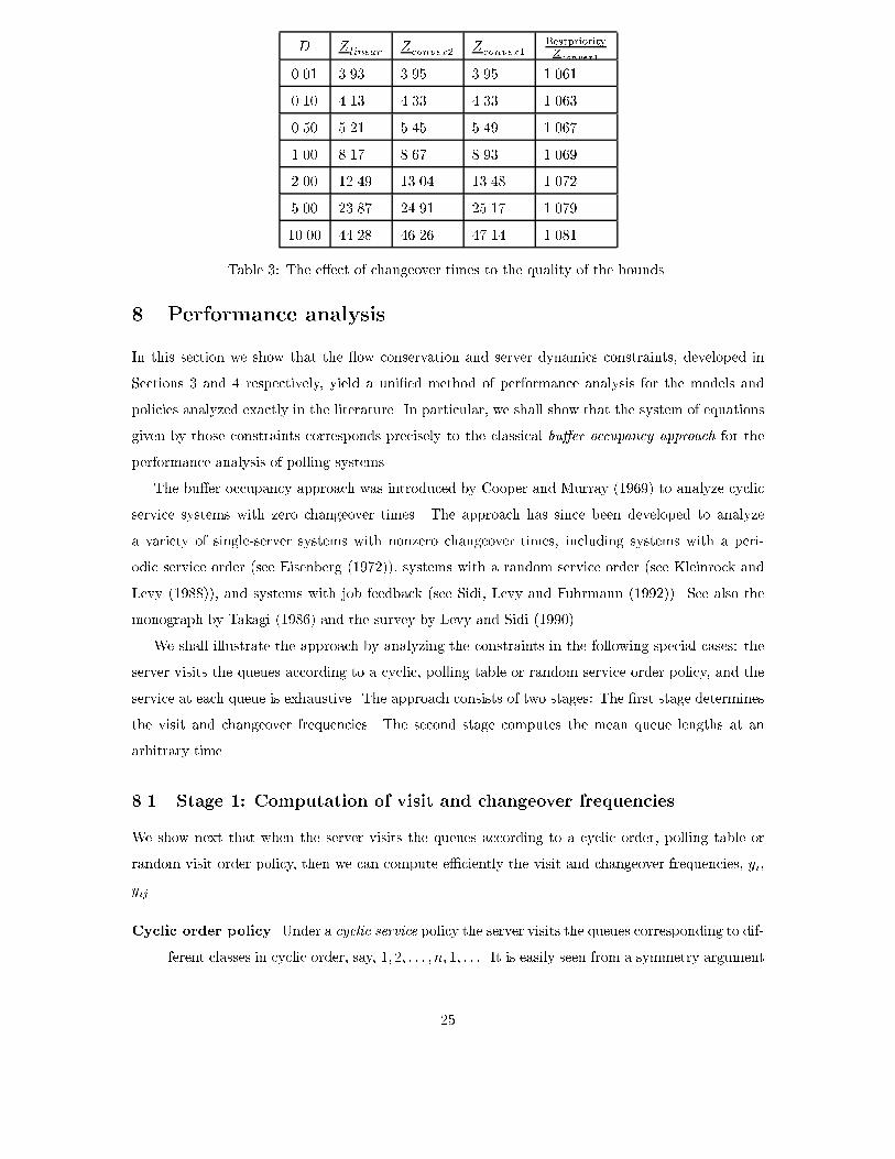
Our next experiment aims at understanding the e�ect of the changeover times. We again have 4

classes, and we have selected parameters as in the previous experiment. We �xed � = 0:8. All the

changeover times were selected equal to the same value D. In Table 3 we report the performance of

the bounds in relation to the best static priority policy as D increases. The quality of the bounds is

relatively insensitive to the value of D, although they slightly worsen with higher changeover times.

24

D Zlinear Zconvex2 Zconvex1BestpriorityZconvex1

0.01 3.93 3.95 3.95 1.061

0.10 4.13 4.33 4.33 1.063

0.50 5.21 5.45 5.49 1.067

1.00 8.17 8.67 8.93 1.069

2.00 12.49 13.04 13.48 1.072

5.00 23.87 24.91 25.17 1.079

10.00 44.28 46.26 47.14 1.081

Table 3: The e�ect of changeover times to the quality of the bounds.

8 Performance analysis

In this section we show that the ow conservation and server dynamics constraints, developed in

Sections 3 and 4 respectively, yield a uni�ed method of performance analysis for the models and

policies analyzed exactly in the literature. In particular, we shall show that the system of equations

given by those constraints corresponds precisely to the classical bu�er occupancy approach for the

performance analysis of polling systems.

The bu�er occupancy approach was introduced by Cooper and Murray (1969) to analyze cyclic

service systems with zero changeover times. The approach has since been developed to analyze

a variety of single-server systems with nonzero changeover times, including systems with a peri-

odic service order (see Eisenberg (1972)), systems with a random service order (see Kleinrock and

Levy (1988)), and systems with job feedback (see Sidi, Levy and Fuhrmann (1992)). See also the

monograph by Takagi (1986) and the survey by Levy and Sidi (1990).

We shall illustrate the approach by analyzing the constraints in the following special cases: the

server visits the queues according to a cyclic, polling table or random service order policy, and the

service at each queue is exhaustive. The approach consists of two stages: The �rst stage determines

the visit and changeover frequencies. The second stage computes the mean queue lengths at an

arbitrary time.

8.1 Stage 1: Computation of visit and changeover frequencies

We show next that when the server visits the queues according to a cyclic order, polling table or

random visit order policy, then we can compute e�ciently the visit and changeover frequencies, yi,

yij .

Cyclic order policy. Under a cyclic service policy the server visits the queues corresponding to dif-

ferent classes in cyclic order, say, 1; 2; : : : ; n; 1; : : :. It is easily seen from a symmetry argument

25

and Proposition 2 that the changeover and visit frequencies are given by

yi = y12 = � � � = yn�1;n = yn1 =1� �

s12 + � � �+ sn�1;n + sn1:

Polling table order policy. Under a polling table policy the server visits queues in a periodic

order given by a sequence T (1); T (2); : : : ; T (m), i.e., it �rst visits class T (1), then class T (2),

etc. Let M(i; j) be the number of i ! j changeovers and let M(i) be the number of server

visits to the i-queue during a cycle in the polling table. Again, a symmetry argument and

Proposition 2 yield

yij = (1� �)M(i; j)P

k 6=l sklM(k; l);

and

yi = (1� �)M(i)P

k 6=l sklM(k; l):

Random visit order policy. Under a random visit order policy (see Kleinrock and Levy (1988))

the server visits the queues in a random order according to Bernoulli routing probabilities:

after visiting the i-queue, it decides to visit next the j-queue with probability rij . Clearly, we

have yij=yi = rij . Combining this relation with Proposition 2 we obtain that the visit and

changeover frequencies are determined by solving the linear system

Xi2N

Xj2Nnfig

sijrijyi = 1� �;

yi =X

j2Nnfig

rjiyj ; for i 2 N :

8.2 Stage 2: Computation of mean queue lengths

Once the visit and changeover frequencies have been determined, the server dynamics constraints de-

veloped in Section 4 become linear. We show next how those constraints yield an exact performance

analysis, by focusing our attention in the special case that the server follows an exhaustive service

policy at each queue (the server continues serving a class until the corresponding queue becomes

empty), and the order in which the server visits the queues is either cyclic or in random order.

In order to compute the vector of mean queue lengths at an arbitrary time, x, we propose the

following three-step procedure:

Step 1. Compute the �rst moments of queue lengths at server visit completion epochs (xHi

j ) by

solving the linear system of size O(n2)

Xk2Nnfig

�yikx

Hi

j � yki(xHk

j + �jski)�= (�j�i + pij � �ij) �i; for i; j 2 N ;

with the additional constraints

xHj

j = 0; for j 2 N :

26

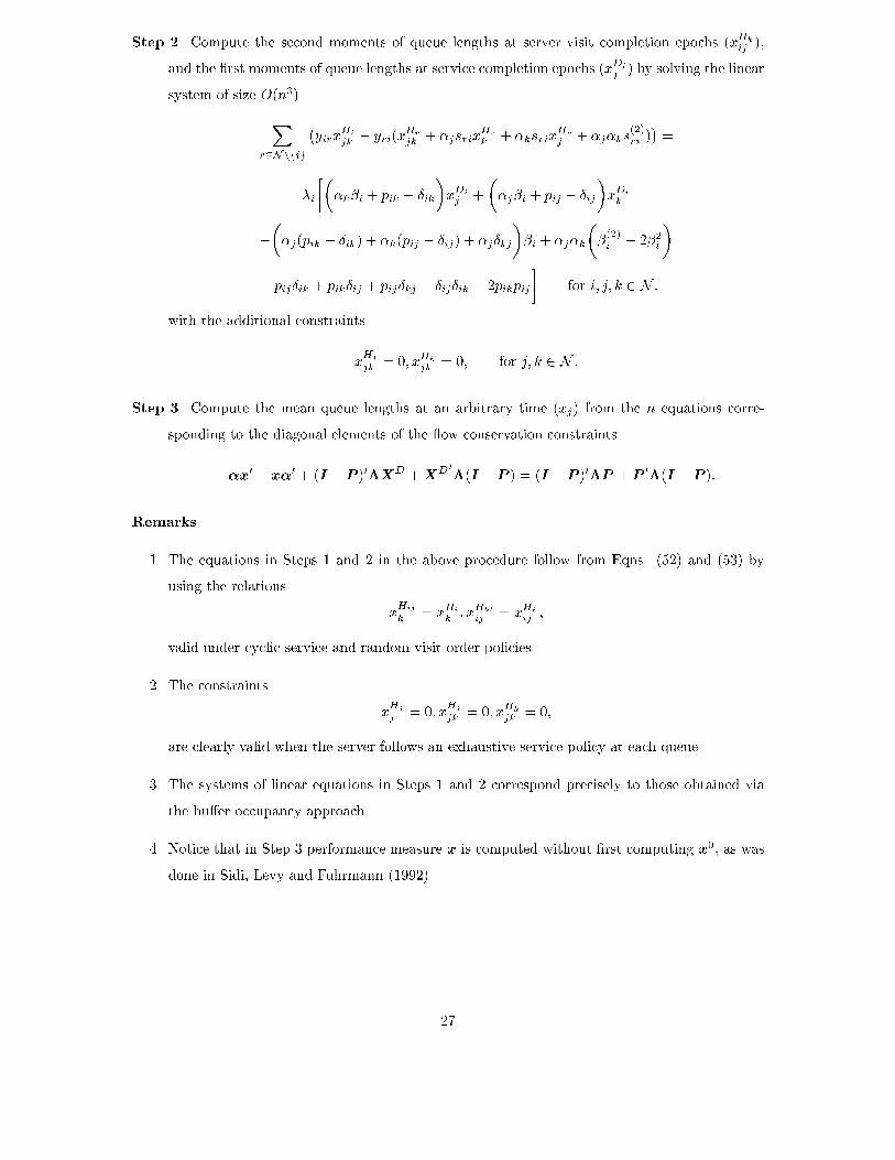
Step 2. Compute the second moments of queue lengths at server visit completion epochs (xHk

ij ),

and the �rst moments of queue lengths at service completion epochs (xDi

j ) by solving the linear

system of size O(n3)

Xr2Nnfig

�yirx

Hi

jk � yri(xHr

jk + �jsrixHr

k + �ksrixHr

j + �j�ks(2)ri )�=

�i

���k�i + pik � �ik

�xDi

j +

��j�i + pij � �ij

�xDi

k

�

��j(pik � �ik) + �k(pij � �ij) + �j�kj

��i + �j�k

��(2)i � 2�2i

�

pij�ik + pik�ij + pij�kj � �ij�ik � 2pikpij

�for i; j; k 2 N :

with the additional constraints

xHj

jk = 0; xHk

jk = 0; for j; k 2 N :

Step 3. Compute the mean queue lengths at an arbitrary time (xj) from the n equations corre-

sponding to the diagonal elements of the ow conservation constraints

��x0 � x�0 + (I �P )0�XD +XD 0�(I �P ) = (I �P )0�P +P

0�(I �P ):

Remarks.

1. The equations in Steps 1 and 2 in the above procedure follow from Eqns. (52) and (53) by

using the relations

xHij

k = xHi

k ; xHkl

ij = xHk

ij ;

valid under cyclic service and random visit order policies.

2. The constraints

xHj

j = 0; xHj

jk = 0; xHk

jk = 0;

are clearly valid when the server follows an exhaustive service policy at each queue.

3. The systems of linear equations in Steps 1 and 2 correspond precisely to those obtained via

the bu�er occupancy approach.

4. Notice that in Step 3 performance measure x is computed without �rst computing x0, as was

done in Sidi, Levy and Fuhrmann (1992).

27

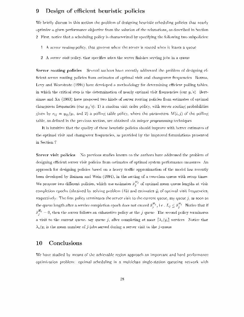
9 Design of e�cient heuristic policies

We brie y discuss in this section the problem of designing heuristic scheduling policies that nearly

optimize a given performance objective from the solution of the relaxations, as described in Section

2. First, notice that a scheduling policy is characterized by specifying the following two subpolicies:

1. A server routing policy, that governs where the server is routed when it leaves a queue.

2. A server visit policy, that speci�es when the server �nishes serving jobs in a queue.

Server routing policies. Several authors have recently addressed the problem of designing ef-

�cient server routing policies from estimates of optimal visit and changeover frequencies. Boxma,

Levy and Weststrate (1991) have developed a methodology for determining e�cient polling tables,

in which the critical step is the determination of nearly optimal visit frequencies (our yi's). Bert-

simas and Xu (1993) have proposed two kinds of server routing policies from estimates of optimal

changeover frequencies (our yij 's): 1) a random visit order policy, with server routing probabilities

given by rij = yij=yi, and 2) a polling table policy, where the parameters M(i; j) of the polling

table, as de�ned in the previous section, are obtained via integer programming techniques.

It is intuitive that the quality of these heuristic policies should improve with better estimates of

the optimal visit and changeover frequencies, as provided by the improved formulations presented

in Section 7.

Server visit policies. No previous studies known to the authors have addressed the problem of

designing e�cient server visit policies from estimates of optimal system performance measures. An

approach for designing policies based on a heavy tra�c approximation of the model has recently

been developed by Reiman and Wein (1994), in the setting of a two-class queue with setup times.

We propose two di�erent policies, which use estimates xHj

j of optimal mean queue lengths at visit

completion epochs (obtained by solving problem (45) and estimates yi of optimal visit frequencies,

respectively: The �rst policy terminates the server visit to the current queue, say queue j, as soon as

the queue length after a service completion epoch does not exceed xHj

j , i.e., Lj � xHj

j . Notice that if

xHj

j = 0, then the server follows an exhaustive policy at the j-queue. The second policy terminates

a visit to the current queue, say queue j, after completing at most d�i=yie services. Notice that

�i=yi is the mean number of j-jobs served during a server visit to the j-queue.

10 Conclusions

We have studied by means of the achievable region approach an important and hard performance

optimization problem: optimal scheduling in a multiclass single-station queueing network with

28

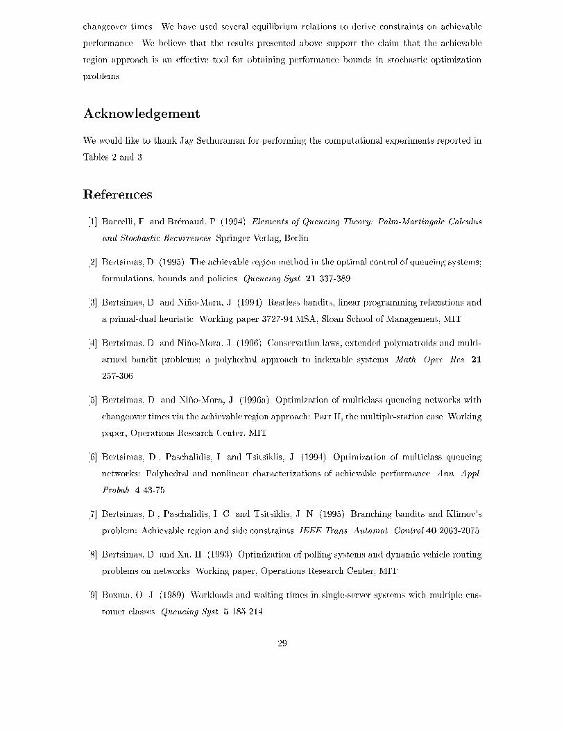
changeover times. We have used several equilibrium relations to derive constraints on achievable

performance. We believe that the results presented above support the claim that the achievable

region approach is an e�ective tool for obtaining performance bounds in stochastic optimization

problems.

Acknowledgement

We would like to thank Jay Sethuraman for performing the computational experiments reported in

Tables 2 and 3.

References

[1] Baccelli, F. and Br�emaud, P. (1994). Elements of Queueing Theory: Palm-Martingale Calculus

and Stochastic Recurrences. Springer-Verlag, Berlin.

[2] Bertsimas, D. (1995). The achievable region method in the optimal control of queueing systems;

formulations, bounds and policies. Queueing Syst. 21 337-389.

[3] Bertsimas, D. and Ni~no-Mora, J. (1994). Restless bandits, linear programming relaxations and

a primal-dual heuristic. Working paper 3727-94 MSA, Sloan School of Management, MIT.

[4] Bertsimas, D. and Ni~no-Mora, J. (1996). Conservation laws, extended polymatroids and multi-

armed bandit problems; a polyhedral approach to indexable systems. Math. Oper. Res. 21

257-306.

[5] Bertsimas, D. and Ni~no-Mora, J. (1996a). Optimization of multiclass queueing networks with

changeover times via the achievable region approach: Part II, the multiple-station case. Working

paper, Operations Research Center, MIT.

[6] Bertsimas, D., Paschalidis, I. and Tsitsiklis, J. (1994). Optimization of multiclass queueing

networks: Polyhedral and nonlinear characterizations of achievable performance. Ann. Appl.

Probab. 4 43-75.

[7] Bertsimas, D., Paschalidis, I. C. and Tsitsiklis, J. N. (1995). Branching bandits and Klimov's

problem: Achievable region and side constraints. IEEE Trans. Automat. Control 40 2063-2075.

[8] Bertsimas, D. and Xu, H. (1993). Optimization of polling systems and dynamic vehicle routing

problems on networks. Working paper, Operations Research Center, MIT.

[9] Boxma, O. J. (1989). Workloads and waiting times in single-server systems with multiple cus-

tomer classes. Queueing Syst. 5 185-214.

29

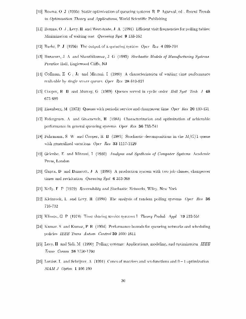
[10] Boxma, O. J. (1995). Static optimization of queueing systems. R. P. Agarwal, ed., Recent Trends

in Optimization Theory and Applications, World Scienti�c Publishing.

[11] Boxma, O. J., Levy, H. and Weststrate, J. A. (1991). E�cient visit frequencies for polling tables:

Minimization of waiting cost. Queueing Syst. 9 133-162.

[12] Burke, P. J. (1956). The output of a queueing system. Oper. Res. 4 699-704.

[13] Buzacott, J. A. and Shanthikumar, J. G. (1993). Stochastic Models of Manufacturing Systems.

Prentice Hall, Englewood Cli�s, NJ.

[14] Co�man, E. G., Jr. and Mitrani, I. (1980). A characterization of waiting time performance

realizable by single server queues. Oper. Res. 28 810-821.

[15] Cooper, R. B. and Murray, G. (1969). Queues served in cyclic order. Bell Syst. Tech. J. 48

675-689.

[16] Eisenberg, M. (1972). Queues with periodic service and changeover time. Oper. Res. 20 440-451.

[17] Federgruen, A. and Groenevelt, H. (1988). Characterization and optimization of achievable

performance in general queueing systems. Oper. Res. 36 733-741.

[18] Fuhrmann, S. W. and Cooper, R. B. (1985). Stochastic decompositions in the M=G=1 queue

with generalized vacations. Oper. Res. 33 1117-1129.

[19] Gelenbe, E. and Mitrani, I. (1980). Analysis and Synthesis of Computer Systems. Academic

Press, London.

[20] Gupta, D. and Buzacott, J. A. (1990). A production system with two job classes, changeover

times and revisitation. Queueing Syst. 6 353-368.

[21] Kelly, F. P. (1979). Reversibility and Stochastic Networks, Wiley, New York.

[22] Kleinrock, L. and Levy, H. (1988). The analysis of random polling systems. Oper. Res. 36

716-732.

[23] Klimov, G. P. (1974). Time sharing service systems I. Theory Probab. Appl. 19 532-551.

[24] Kumar, S. and Kumar, P. R. (1994). Performance bounds for queueing networks and scheduling

policies. IEEE Trans. Autom. Control 39 1600-1611.

[25] Levy, H. and Sidi, M. (1990). Polling systems: Applications, modeling, and optimization. IEEE

Trans. Comm. 38 1750-1760.

[26] Lov�asz, L. and Schrijver, A. (1991). Cones of matrices and set-functions and 0�1 optimization.

SIAM J. Optim. 1 166-190.

30

[27] Ni~no-Mora, J. (1995). Optimal Resource Allocation in a Dynamic and Stochastic Environment:

A Mathematical Programming Approach. PhD Dissertation, Sloan School of Management, MIT.

[28] Papadimitriou, C. H. and Tsitsiklis, J. N. (1994). The complexity of optimal queueing network

control. Working Paper LIDS 2241, MIT.

[29] Papangelou, F. (1972). Integrability of expected increments and a related random change of

time scale. Trans. Amer. Math. Soc. 165 483-506.

[30] Reiman, M. I. and Wein, L. M. (1994). Dynamic scheduling of a two-class queue with setups.

Working paper, Sloan School of Management, MIT.

[31] Shanthikumar, J. G. and Yao, D. D. (1992). Multiclass queueing systems: Polymatroidal struc-

ture and optimal scheduling control. Oper. Res. 40 S293-299.

[32] Sidi, M., Levy, H. and Fuhrmann, S. W. (1992). A queueing network with a single cyclically

roving server. Queueing Syst. 10 121-144.

[33] Takagi, H. (1986). Analysis of polling systems. MIT Press, Cambridge, MA.

[34] Tsoucas, P. (1991). The region of achievable performance in a model of Klimov. Research Report

RC16543, IBM T.J. Watson Research Center, Yorktown Heights, NY.

[35] Vandenberghe, L. and Boyd, S. (1996). Semide�nite programming. SIAM Review 38 49-95.

31