Embed Size (px)
Citation preview

Loughborough UniversityInstitutional Repository
Optimization of life-cyclemaintenance of deteriorating
bridges with respect toexpected annual systemfailure rate and expected
cumulative cost
This item was submitted to Loughborough University's Institutional Repositoryby the/an author.
Citation: BARONE, G., FRANGOPOL, D.M. and SOLIMAN, M., 2014. Op-timization of life-cycle maintenance of deteriorating bridges with respect to ex-pected annual system failure rate and expected cumulative cost. Journal ofStructural Engineering, 140 (2), 04013043.
Additional Information:
• This is the author's version of a work that was accepted for publication inJournal of Structural Engineering. A definitive version was subsequentlypublished at: http://dx.doi.org/10.1061/(ASCE)ST.1943-541X.0000812
Metadata Record: https://dspace.lboro.ac.uk/2134/16760
Version: Accepted for publication
Publisher: c© American Society of Civil Engineers (ASCE)
Rights: This work is made available according to the conditions of the Cre-ative Commons Attribution-NonCommercial-NoDerivatives 4.0 International(CC BY-NC-ND 4.0) licence. Full details of this licence are available at:https://creativecommons.org/licenses/by-nc-nd/4.0/
Please cite the published version.

1
Optimization of life-cycle maintenance of deteriorating bridges
considering expected annual system failure rate and expected
cumulative cost
Giorgio Barone1, Dan M. Frangopol, Dist. M.ASCE2* and Mohamed Soliman, S.M.ASCE3
Abstract Civil infrastructure systems are subjected to progressive deterioration resulting from multiple
mechanical and environmental stressors. This deterioration process is developed under
uncertainties related to load effects, structural resistance, and inspection outcomes, among
others. In this context, life-cycle optimization techniques provide a rational approach to
manage these systems considering uncertainties as well as several budgetary and safety
constraints. This paper proposes a novel optimization procedure for life-cycle inspection and
maintenance planning of aging structures. In this procedure, the structural system effects are
accounted for by modeling the structure as a series, parallel, or a series-parallel system whose
components are subjected to time-dependent deterioration phenomena. Different possible
repair options are considered depending on the damage state and the outcomes of each
inspection. For each component, essential or preventive maintenance aiming at reducing the
system failure rate, are performed when inspection results indicate that the prescribed
threshold damage levels have been reached or violated. Otherwise, no repair is performed.
Optimum inspection and maintenance plans are formulated by minimizing both the expected
system failure rate and expected cumulative inspection and maintenance cost over the life-
cycle of the structure. The proposed approach is applied to an existing bridge.
ASCE Subject Headings: optimization; deterioration; inspection; maintenance.
Author keywords: optimization; life-cycle management; inspection and maintenance
planning; deteriorating structures; failure rate; uncertainties. 1Research Associate, Department of Civil and Environmental Engineering, Engineering Research Center for Advanced Technology for Large Structural Systems (ATLSS Center), Lehigh University, 117 ATLSS Dr., Bethlehem, PA 18015-4729, USA, [email protected]. 2Professor and the Fazlur R. Khan Endowed Chair of Structural Engineering and Architecture, Department of Civil and Environmental Engineering, Engineering Research Center for Advanced Technology for Large Structural Systems (ATLSS Center), Lehigh University, 117 ATLSS Dr., Bethlehem, PA 18015-4729, USA, [email protected], *Corresponding Author. 3Graduate Research Assistant, Ph.D. Candidate, Department of Civil and Environmental Engineering, Engineering Research Center for Advanced Technology for Large Structural Systems (ATLSS Center), Lehigh University, 117 ATLSS Dr., Bethlehem, PA 18015-4729, USA, [email protected].

2
Introduction
Civil infrastructure systems are continuously subjected to aging phenomena. The separate or
combined effects of resistance reduction and/or increase of loads over time lead to a
reduction of structural safety. Cost-effective maintenance strategies are needed to guarantee
adequate structural reliability levels with respect to different limit states. Decision-making
processes for the development of optimal maintenance plans have to consider all epistemic
and aleatory uncertainties that may affect the structure during its life-cycle. Life-cycle
probabilistic concepts and methods for the determination of lifetime maintenance plans of
deteriorating structures have been largely discussed in recent years and several approaches
have been proposed. These concepts and methods are able to establish well-balanced
intervention schedules that consider various economic and safety requirements while taking
into account uncertainties associated with the time-dependent structural performance. An
extensive review of such methods is reported in both Frangopol and Liu (2007) and
Frangopol (2011). The main approaches are based on (a) probabilistic performance
indicators, (b) risk assessment, or (c) lifetime distribution functions.
With regard to probabilistic performance indicators, the reliability index is recognized
to be highly effective for maintenance planning of deteriorating structures. This has been
discussed in several papers using decision-tree analysis [Estes and Frangopol 2003], single
objective optimization [Mori and Ellingwood 1994], or multi-objective optimization [Orcesi
and Frangopol 2011(a)]. While the reliability index is related to the annual probability of
failure of the structure, a different indicator can be used considering also economic losses due
to failure by using risk-based maintenance planning. Risk-based decision making takes into
account both the direct losses associated with failure (e.g. repair or rebuilding costs)
[Ramirez et al.2012] and the indirect losses caused by the nonoperational state of the system
[Ang and Tang 1984]. Components subjected to higher risk should have top priority for
maintenance interventions. Arunraj and Maiti (2007) classify risk-based maintenance
techniques based on quantitative or qualitative nature of the risk assessment, type of
applications, and input and output data types.

3
Although the reliability index and risk, defined in general as a function of the annual
failure probability, are associated with a specific point-in-time, lifetime distributions keep
memory of the events on the system during the structural life-cycle. Optimal maintenance
planning using lifetime distribution functions has been proposed considering single and
multi-objective optimization based on system survivor function [Orcesi and Frangopol
2011(b), Okasha and Frangopol 2010]. Failure rate has been considered for preventive
maintenance planning of series systems [Caldeira Duarte et al. 2006] and
inspection/preventive maintenance schedules have been proposed for a gantry crane using a
coupled Bayesian network [Baek et al. 2009]. Failure rate gives the probability of structural
failure within a prescribed time interval conditioned on the structural survival up to this time
interval. Additionally, it gives an indication on the rate of decrease in the structural
reliability, an attribute that makes it a valuable indicator in forecasting the structural
performance for life-cycle planning purposes. Recently, Barone and Frangopol (2013)
proposed a component-based procedure for determining optimal lifetime inspection/repair
plans for deteriorating structures based on the definition of thresholds for the hazard function
and using one type of repair (i.e. replacing the damaged component). Their procedure
considered a single objective optimization with the goal of minimizing the lifetime hazard
function where the output is the optimum number of inspections and their optimal application
times.
In this paper, a multi-objective optimal inspection and maintenance planning
approach for structural systems subjected to aging phenomena, focusing on the annual failure
rate and life-cycle maintenance cost, is proposed. The approach is system-based, in which the
interaction of components in the system is considered by modeling the structural
configuration as series, parallel, or series-parallel. Two different types of repair are
considered in which the selection of the appropriate repair action is based on inspection
outcomes and predefined damage level thresholds. For each structural component, when the
damage level exceeds a certain threshold, essential maintenance is performed, in which total
restoration of the initial component performance is achieved. For minor deterioration levels,
preventive maintenance is considered, aiming at arresting the progress of the deteriorating

4
phenomena acting on the structure for a period of time. Finally, when the inspection results
report negligible damage levels, no repair is performed. Accuracy of inspection is taken into
account as a function of the imperfections affecting inspection results. A bi-objective
optimization is proposed to minimize both the maximum expected system failure rate over
the life-cycle of the system and the expected total cost of all inspection and maintenance
actions. Optimal solutions are determined for a given total number of inspections/repairs and
inspection accuracy. The proposed approach is applied to an existing bridge considering the
effects of deterioration due to corrosion of the girders and of the reinforcement bars of the
concrete deck.
Inspection and maintenance options
Maintenance planning is subjected to several uncertainties related to structural deteriorating
phenomena, loadings, quality of inspection procedures, and decisions regarding maintenance
types and their costs, among others. Damage assessment through inspections dictates the
choice between repairing the structure or not, and eventually what degree of maintenance
should be performed. Advanced degradation of the structural performance requires costly
repairs aimed to considerably improve the structural reliability, while preventive maintenance
may be applied if the structure has still an acceptable service level, reducing the failure rate
of the structure with low-cost interventions. Moreover, when the degradation effects are
marginal it may be decided not to perform any maintenance actions.
Several inspection techniques exist for assessment and performance prediction of
bridges. Visual inspections and non-destructive testing are the most common ones. Visual
inspections are primarily performed to estimate structural performance using condition
indexes for management decisions. Non-destructive techniques can provide excellent results
but, due to their cost, they are usually scheduled at specific times for a particular concern
[Frangopol 2011]. Decision on which inspection technique should be applied is dependent on
the structure, the desired accuracy, and the cost that can be afforded. Well-timed inspections
followed by correct repair decisions may effectively lead to consistent extensions of the
lifetime of structures.

5
In general, visual inspections take place at regular time intervals. Herein, detailed in-
depth inspections are considered. Non-destructive techniques are used to obtain detailed data
about the structural deterioration state of bridge components. Several techniques (e.g. half-
cell potential tests, infrared thermography, ground penetrating radar, among others) have
been developed in recent years, each one having its own advantages, costs and applicability
[Carino 1999, Clark et al. 2003, Wang et al. 2011].
In this paper, the effect of the degradation is modeled as a continuous reduction of the
structural capacity (resistance) iR t of the components over time. A rational way to quantify
structural capacity over time is to use a probabilistic approach that takes into account
imperfections related to the predictive model arising from uncertainties associated with
material and structural properties and with the deterioration phenomena that affect the
structure. In-depth inspections are able to identify the damage level and, therefore, provide an
estimation of the residual capacity of the components at the inspection time. On the other
hand, inspection results are affected by imperfections in which the measurement error can be
considered to follow a normal distribution with zero mean. Taking into account both the
imperfections associated with the structural resistance prediction and the inspection result, the
estimated capacity estiR for the component i immediately after inspection time inspt is a
random variable having the mean of the predicted structural capacity at that time iR inspt
and standard deviation iinsp insp R inspk t , where
iR is the standard deviation of the
resistance accounting for the imperfections associated with the predictive model and 1inspk
is an index of the inspection accuracy with 1inspk if no inspection imperfections are
considered (i.e., perfect inspection). Sensitivity of solutions to quality of different inspection
techniques was reported in Kim et al. (2013).
Three possible repair options are considered for each component, based on the in-
depth inspection result estiR . In particular, two different thresholds for essential and
preventive maintenance, namely ,EM i and ,PM i , where , .EM i PM i , are given for each
component to determine the appropriate repair option based on its initial capacity. Essential
maintenance, herein defined as total restoration of the component performance to its original
value, is performed when ,
esti EM iR . Preventive maintenance is, instead, applied if the

6
estimated component capacity is between the two thresholds, i.e. , ,
estEM i i PM iR . It is
considered that the effect of the preventive maintenance is to block the effects of the aging
phenomena for a certain period, that is the residual capacity remains constant for a given
interval of time. The effects of preventive and essential maintenances on the residual capacity
are qualitatively represented in Figures 1(a) and 1(b), respectively. Finally, no repair is
considered if ,
esti PM iR . Therefore, for each component i , the probability of essential
maintenance ,EM iP , preventive maintenance ,PM iP , or no repair ,NR iP after one inspection at a
given instant of time can be evaluated by integration of the probability density function
(PDF) of the estimated residual capacity , ,R if x t , as:
,
,
,
, ,0
, ,
, , ,
,
,
1
EM i
PM i
EM i
EM i R i
PM i R iR
NR i EM i PM i
P t f x t dx
P t f x t dx
P t P t P t
(1)
These probabilities are graphically represented as the areas shown in Figure 1(c).
When sequences of inspection/repair are considered, the set of possible events that
may occur can be represented by an event tree model in which each branch is associated with
a sequence of essential or preventive maintenance, or inspections with no repair. Each branch
has a probability of occurrence BkP , where k is the branch number. Since the tree
represents the set of all possible events, obviously 1
B 1bN
kk
P
, where bN is the total
number of branches. Figure 2 shows the event tree associated with a single component
subjected to two inspections. Possible repair options following each inspection are shown
together with the probability associated with each branch. In general, given a system with CN
components and ON possible repair options for each component, the total number of different
branches after inspN inspection is given by insp CN N
b ON N .

7
Expected annual failure rate and expected total maintenance cost
For the determination of optimal inspection and maintenance times, several approaches can
be used, based on various performance indicators, including reliability index, risk, or lifetime
functions. In this paper, attention has been focused on the average system failure rate sysh t ,
defined as the probability of failure occurring between t and t t , given that the system
survives at the time instant t , and averaged over the interval , t t t [Leemis 1995]:
|F Fsys
P t T t t T th t
t
(2)
The average system failure rate may be rewritten in terms of system survivor function
sysS t representing the probability of the system being functional at any time t :
sys FS t P T t (3)
in which FT is the time of failure occurrence. Therefore, the average system failure rate is:
sys syssys
sys
S t S t th t
S t t
(4)
The use of this function allows taking advantage of the conditional failure time probability,
giving additional information with respect to other performance indicators, such as the point-
in-time reliability index. As 0t , Eq. (4) becomes the instantaneous failure rate, which is
by definition the hazard function.
For the applications examined in this paper, the annual system failure rate has been
considered. First the point-in-time annual probability of failure has been evaluated by using
the software RELSYS (RELiability of SYStems) [Estes and Frangopol 1998]. The point-in-
time probability of system failure is the probability of violating any of the limit state
functions that define its failure modes. The limit state function is defined as:

8
0g t R t Q t (5)
where R t and Q t are the resistance and load effect at t , respectively. Based on this
limit state, the point-in-time probability of failure can be evaluated as:
any 0sysP t P g t (6)
For a series-parallel system, RELSYS first computes the failure probability of all its
components. Then, the system is progressively reduced to simpler equivalent subsystems
(i.e., having the same reliability of the initial system), until a single equivalent component
remains. Once the point-in-time annual failure probability sysP t for the system is known,
the time-dependent failure probability at the year nt can be evaluated as [Decò and Frangopol
2011]:
1
11 1
1in
sys n sys i sys ji j
TDP t P t P t
(7)
where sysTDP represents the cumulative distribution function of the system time-to-failure.
Hence, by definition, the system survivor function is:
1sys sysS t TDP t (8)
Finally, by considering Eqs. (4) and (8), the annual system failure rate at the year nt is:
1
1sys n sys n
sys nsys n
TDP t TDP th t
TDP t
(9)
To determine the optimal set of maintenance times for structural systems, taking into
account different maintenance options based on in-depth inspection results, it is necessary to
keep track of all possible actions and their occurrence probabilities. Obviously, preventive
and essential maintenance provide a reduction of the annual system failure rate. The

9
magnitude of this reduction depends on the repair times, deterioration rate of the structural
capacity, and loading conditions.
For example, considering a single component subjected to an increasing axial force
and a cross-sectional area reduction over time, the structural failure probability can be
assessed using the following performance function:
yg t A t f L t (10)
where A t and L t
represent the time-variant cross-sectional area and axial load,
respectively, and yf is the yield strength of the component material. For illustrative purposes,
a deterministic deterioration model, consisting in a continuous loss of cross-sectional area
over time, is here considered [Okasha and Frangopol 2009]. The cross-sectional area A t is
assumed to be a random variable with mean A t and standard deviation A t given by:
1 0
0.03 1 0
t
A
t
A
t DR A
t DR A
(11)
where 0A is the initial cross-sectional area and DR is the deterioration rate. The load L t
is modeled as a random variable with mean:
1 0t
L t l L (12)
and coefficient of variation (COV) of 5%, where 0L is the initial load and l is the load
increase parameter. The annual failure rates resulting from performing two inspections after
15 and 25 years of service are presented in Figure 3(a) for three possible branches of the
associated event tree (Figure 2). The initial cross-sectional area 0A and the annual
deterioration rate DR are considered to be 3.0 cm2 and 2x10⁻³, respectively, whereas initial
load and its annual increase rate are assumed 60 kN and 2x10⁻⁴, respectively. The yield stress

10
follows a lognormal distribution with parameters shown in Table 1, and A t and L t are
assumed Gaussian.
The annual failure rate profiles in Figure 3(a) show the effect of essential maintenance
(restoring the structural resistance to the initial value) and preventive maintenance
(precluding the further degradation in the structural resistance for an effective period of 5
years). As shown, the annual failure rate varies considerably among the different branches
after the first inspection. With the aim of representing the effect of the maintenance plan, in
an efficient way, by means of a single function that takes into account all the possible events
(i.e. preventive or essential maintenance or no repair at each inspection time), the expected
annual failure rate, obtained as the summation of the annual failure rates associated with each
branch and weighted by their occurrence probabilities BkP , is:
,1
BbN
sys k sys kk
E h t P h t
(13)
where bN is the total number of branches and ,sys kh t is the annual failure rate associated
with branch k .
When dealing with inspection and maintenance planning optimization, monitoring of
cumulative costs over time is crucial. Analogously to the expected annual failure rate, it is
convenient to consider the expected total cost of the maintenance plan, obtained as:
1
BbN
tot k kk
E C P C
(14)
kC is the total cost of branch k , obtained by summing inspection cost, as well as preventive
and essential maintenance costs for the considered branch:

11
1 1 11 1 1
insp PM EM
i j jinsp PM EM
PM EMN insp N Nj j
k t t ti j j
d d d
C CCC
r r r
(15)
where inspC is the inspection cost, PMjC and EM
jC are the costs of the j-th preventive and
essential maintenance actions, respectively, iinspt is the i-th inspection time, j
PMt and jEMt are
the j-th preventive and essential maintenance times, respectively, and dr is the annual
discount rate of money, introduced to convert the future monetary value of inspections and
repairs, performed at different times, to the present one. In the following, it has been assumed
that 0dr .
Probabilities of occurrence of the branches B kP for the single component, used to
evaluate the expected annual failure rate and expected total cost, are next calculated
considering the estimate residual cross-sectional area of the component estA resulting from
the in-depth inspection outcomes. Two thresholds EM and PM are defined with respect to
the initial cross-sectional area of the component to determine the appropriate maintenance
type. In particular, for the single component example, three different threshold sets have been
considered as follows:
threshold T1: , 1 0.95 0EM T A ; 0.98 0PM A
threshold T2: , 2 0.90 0EM T A ; 0.98 0PM A
threshold T3: , 3 0.85 0EM T A ; 0.98 0PM A
Constraints for performing essential or preventive maintenance are , i
estEM TA
and
, i
estEM T PMA , respectively. Otherwise, no repair is considered. Therefore, for the
threshold set T1, if the inspection reveals that the residual area is less than 0.95 0A ,
essential maintenance has to be performed. Additionally, if the residual area obtained by
inspection results is between 0.95 0A and 0.98 0A , preventive maintenance is performed.

12
Finally, if the residual area is more than 0.98 0A no repair is performed after the
inspection.
Figure 3(b) illustrates expected annual failure rates for the three threshold sets T1, T2
and T3, assuming inspections to be performed at 15 and 25 years. By increasing EM , the
probability of performing essential or preventive maintenance is increased or reduced,
respectively. Therefore, between the three considered scenarios, T1 is characterized by the
lowest expected annual failure rate and the highest expected total cost.
Bi-objective optimization for determining the optimal life-cycle
maintenance plan
A bi-objective optimization procedure is herein proposed to determine the optimal
maintenance plan of a multi-component structural system using the lifetime maximum
expected system failure rate and the expected total cost as objective functions. To define the
optimization problem, an observation time window tott , as well as the total number of
inspections inspN in the lifetime plan, have to be prescribed. The performance functions
ig t for the system components and the in-depth inspection and repair costs have to be
defined. Finally, for the proposed model, results will be dependent on the in-depth inspection
accuracy.
Based on these assumptions, the Pareto-optimal solution front [Deb 2001] of
maintenance plans can be obtained as the solution of the following optimization problem:
Given: , , , , , ,insp PM EMtot insp i i i inspt N g t C C C k (16)
Find: 1 , , inspN
insp insp inspt tt (17)
To minimize:
max max
0sys
tot
tot
h E h tt t
E C
(18)

13
Such that: 1 1,...,k kinsp insp PM inspt t T k N (19)
where inspC ,
PMiC and EM
iC are the inspection, preventive and essential maintenance
costs, respectively, and inspk is the constant associated with the inspection accuracy
previously introduced. The constraints in Eq. (19) have been added to guarantee that, on
average, a new preventive maintenance is not performed before the effect of the previous one
has ended.
Three different configurations of three-component systems, shown in Figure 4(a),
have been studied. The system models cover the series, series-parallel, and parallel
configurations. For the i-th component of each system, the performance function has been
defined, analogously to the single-component example, through Eqs. (10) – (12), taking into
account the cross-sectional area loss of the components and the increase of loads over time.
Values for the initial cross-sectional areas 0iA , deterioration rates iDR , initial load 0L
and coefficient l , as well as mean and COV of the components yield stresses ,y if are
reported in Table 1. Cross-sectional areas of the components are considered uncorrelated,
while perfect correlation is assumed between their yield stresses.
For the three systems, presented in Figures 4(a), annual probabilities of failure for
components and systems obtained by RELSYS are plotted in Figure 4(b). As expected, the
parallel system yields the lowest annual probability of failure among the three systems.
Additionally, for the series-parallel system, the system performance is highly dependent on
the behavior of the third component. Figures 5(a), (b), and (c) depict the annual system
failure rate of the three structural system models considering an in-depth inspection
performed at 20 years of service. Each profile has 27 different repair options after the first
inspection, namely no repair, preventive maintenance, and essential maintenance for each of
the three components. As shown in Figure 5(b) for the series-parallel system, among the 27
possible branches, it is possible to distinguish three groups related to the maintenance options
(i.e., no repair, preventive, essential maintenance) of the critical component (i.e., component
3), whereas for the series or parallel systems, it is not easy to identify these distinctive
groups. Therefore, when considering the series-parallel system, although the number of

14
branches increases exponentially with the number of components, it is possible to reduce the
number of analyzed scenarios focusing the attention exclusively on the most critical
components.
Figures 6 (a), (b) and (c) show the expected system failure rate, obtained by Eq. (13),
for the series, series-parallel, and parallel systems, respectively. The profiles are associated
with the predefined threshold sets T1, T2, and T3 for determining the maintenance type at
each inspection.
The bi-objective optimization problem defined by Eqs. (16)-(19) has been solved for
the three systems considering two in-depth inspections during 40 years. For the in-depth
inspection accuracy 1.3inspk has been considered for the three systems. The two thresholds
governing the probability of occurrence of the essential and preventive maintenance for each
component have been selected as , 0.90 0EM i iA and , 0.98 0PM i iA , respectively.
These selected thresholds correspond to the previously defined threshold set T2. Nominal
costs of 1, 10 and 100 have been considered for inspection, preventive and essential
maintenance, respectively.
The defined optimization problem has been solved by means of genetic algorithms
(GAs), using the global optimization toolbox provided in MATLAB 2012b. Multi-objective
GAs provide Pareto fronts of optimal solutions, representing a set of maintenance schedules
constituting dominant solutions with respect to the chosen objectives. MATLAB toolbox
utilizes a controlled elitist genetic algorithm, that is a variant of NSGA-II [Deb 2001]. Single
point crossover has been used, and the optimization has been performed considering an initial
population size of 150 solutions and 200 maximum iterations. The objective function has
been implemented to evaluate first the annual failure probability of the system for each
branch of the event tree, by using RELSYS software. Average system failure rates are
computed by Eqs. (7) and (9). Finally, maximum expected system failure rate and the
expected total cost are obtained by Eqs. (13) and (14). In order to increase the computational
efficiency, branches with occurrence probability 4B 10kP have been discarded, since
they have negligible contribution towards the evaluation of the expected system failure rate.
The bookkeeping technique described in Bocchini and Frangopol (2011) has been used to

15
further improve the computational efficiency of the routine. Briefly, the objective function
has been implemented so that when a new solution is evaluated, it is automatically stored into
a table. For each set of design variables, the GA routine checks first if it is possible to retrieve
immediately the solution from the table instead of evaluating the objective function itself.
Figure 7(a) depicts the Pareto front obtained for the three systems considering two in-
depth inspections ( 2inspN ). As the three Pareto fronts indicate, maximum expected system
failure rate varies significantly with respect to the system configuration. Between the three
considered systems, the parallel one has the lowest failure probability, and consequently the
lowest maximum expected system failure rate. On the contrary, the highest values of the
maximum expected system failure rate are associated with the series system. Three particular
solutions X , X and X of the Pareto fronts shown in Figure 7(a) are reported in detail in
Table 2. These solutions have been chosen so that they have the same expected total cost. The
series and series-parallel systems optimal solutions require shorter time intervals between the
two in-depth inspections, compared to the parallel system.
For each system configuration, the percentage of increase in total cost C between
the cheapest and the most expensive optimal solutions in the corresponding Pareto front is
computed as:
min max
mintot tot
tot
E C E CC
E C
(20)
and the corresponding percentage of reduction in the maximum expected annual system
failure rate h as:
max max
max
max min
max
h hh
h
(21)
where maxh is the maximum expected annual system failure rate. Figure 7(b) presents the
values of C and h for the three different systems considered in this section. For this
particular example, the series system shows the largest C coupled with the smallest h ,

16
among the three systems. In contrast, the highest h is achieved for the series-parallel
system. This occurs since the three high-cost optimal solutions involve inspection times in the
second half of the system life-cycle, maximizing the probability of performing maintenance
on the component with highest deterioration rate (i.e., component 3 in Figure 4(a)). This
component has the most critical position in the series-parallel configuration.
Case study: Colorado State Highway Bridge E-17-AH
As a case study, the proposed method has been applied to the superstructure of the
Colorado State Highway Bridge E-17-AH. The bridge reinforced concrete deck is supported
by nine steel girders and its cross-section is presented in Figure 8(a). A detailed description of
the bridge was given in [Estes 1997]. Considering the superstructure symmetry and that
failure of the system is reached by either failure of the deck or any two adjacent girders, the
bridge has been studied as the series-parallel model composed by deck and 5 girders shown
in Figure 8(b). Neglecting the dead load due to the weight of the structure itself, limit state
functions for deck and girders are as follows [Estes 1997]:
2 2
0.563 0244.8
ydeck y d deck
c
A t fg A t f M t
f
(22)
, , 0gir i i y g i gir ig Z t F IM t (23)
where A t and yf are the cross-sectional area and yield strength of the deck reinforcement
bars, respectively; cf is the 28-day compressive strength of deck concrete; iZ t is the
plastic section modulus of the girder i; yF is the yield strength of the steel girders; deckM t
and ,gir iM t are, respectively, the moments acting on the deck and girder i, due to traffic
loads; i and I are the traffic load distribution factor and impact factor of girders,
respectively; d and g are modeling uncertainty factors of the resistance of deck and
girders.

17
Load effects and corrosion of deck reinforcement bars and girders have been modeled
following the data provided by Estes (1997). For the deck reinforcement bars, a uniform
corrosion is assumed. The residual area of the reinforcement bars is:
2
4 bar barA t n d t
(24)
where barn is the number of reinforcement bars in the deck and bard t is the bar diameter at
time t which is expressed as
0 0.0203bar corr inid t d i t T (25)
where 0d is the initial diameter, corri represents the rate of corrosion parameter, and iniT is
the initiation time of corrosion. For the steel girders, the corrosion propagation model
proposed by Albrecht and Naeemi (1984) is assumed. Structural loads are evaluated as
indicated in Estes (1997). Parameters for the traffic load moment distribution are obtained
considering the average daily truck traffic on the bridge and are discussed in details in Estes
(1997) and Akgül (2002). The random variables involved in the limit state functions in Eqs.
(22) and (23) are reported in Table 3. The series-parallel system of the bridge represented in
Figure 8(b) has been analyzed by means of RELSYS software, and the annual failure
probability sysP t of the system and its components is plotted in Figure 8(c). As shown, after
50 years of service, the system failure probability is mostly controlled by the reliability of the
reinforced concrete deck.
For the determination of the optimum maintenance plan, different possible actions
have been considered for deck and girders. Regarding the deck, it has been assumed that the
in-depth inspections are able to identify the corrosion penetration in the deck and, therefore,
to estimate the residual diameter of the reinforcement bars at the inspection time estbard . Thus,
the estimated residual cross-sectional area of the bars estA t is obtained by Eq. (24). Three
possible actions have been considered for the deck: essential or preventive maintenance, and
no repair. As stated in the previous section, probability of occurrence of the different repair

18
options is dictated by two thresholds, that have been defined in terms of initial mean of the
cross-sectional area of the reinforcement bars at the initial time 0A :
, 0.90 0EM deck A ; , 0.98 0PM deck A (26)
Essential maintenance is performed when the estimated bar cross-sectional area is less then
,EM deck , while preventive maintenance is applied if , ,
estEM deck PM deckA . No repair is
considered in the remaining cases. The essential maintenance is assumed to completely
restore the initial performance of the deck, while the preventive maintenance keeps the areas
of reinforcement bars unchanged (i.e., corrosion is blocked) for the next five years.
In the case of the girders, resistance over time depends on the plastic section modulus
iZ t . Therefore, it has been considered that the in-depth inspection estimates the depth of
corrosion in the girder and then, based on Estes (1997), the residual plastic section modulus
estiZ t . Only the preventive maintenance option has been considered to be performed when
the estimated plastic section modulus is less than 98% of the mean initial one. Otherwise, no
repair is performed. Essential maintenance of the girders does not significantly reduce the
failure probability of the superstructure, as shown in Figure 8(d) where the annual system
failure probabilities of the structure without maintenance, with essential maintenance on the
deck, and essential maintenance on the girders at 30 years are compared. Therefore, such an
expensive but not so effective option has not been included in the possible maintenance
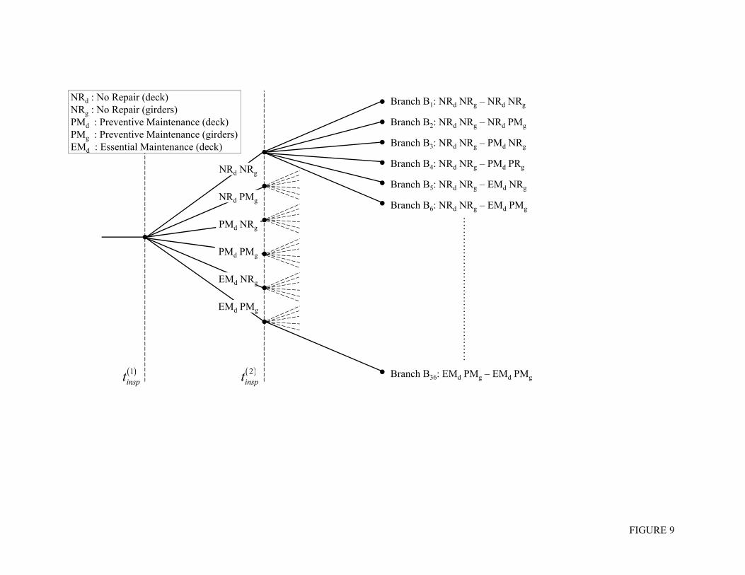
plans. The event tree associated with all possible repair options after one inspection is
illustrated in Figure 9.
Cost of essential maintenance on the deck is $225,600 corresponding to the cost of
deck replacement, based on data provided by Estes (1997). For preventive maintenance on
the deck and girders, costs have been assumed as $40,000 and $75,000, respectively. In-depth
inspection cost for the bridge superstructure depends on the accuracy of the inspection itself.
High accuracy inspection will, necessarily, be more expensive. Therefore, in-depth cost
inspection has been computed as:

19
1
*insp
insp kC C (27)
where *C =$50,000 has been assumed as cost of an ideal inspection (i.e., not subjected to any
error), and 1inspk is the index associated with the inspection accuracy.
The Pareto front of optimal maintenance plans for the bridge has been determined as
the solution of the optimization problem described by Eqs. (16) – (19). The minimum interval
between two successive in-depth inspections, PMT , is, in this case, 5 years.
1 5 1,...,k kinsp insp inspt t years k N (28)
GAs and RELSYS have been used for determining the Pareto-optimal solutions for the bi-
objective optimization problem. Figure 10 shows the Pareto front obtained considering two
in-depth inspections ( 2inspN ), index of inspection accuracy 1.3inspk , and, therefore, using
Eq. (27), inspection cost $4, 200inspC . Three representative solutions, A, B and C, are
selected in Figure 10 and reported in details in Table 4 and Figure 11. The annual system
failure rate associated with the three solutions is presented in Figures 11(a), (c), and (e). In
particular, the expected system failure rate is compared to the annual system failure rate of
the two branches with the highest probability of occurrence. Additionally, the expected
cumulative cost profiles of solutions A, B, and C are compared with cumulative cost profiles
of the two branches having the highest probability of occurrence in Figures 11(b), (d), and (f).
As shown in Figure 11, optimal solutions with low expected total cost are
characterized by early maintenance times. These solutions are selected by the optimizer since
the need for essential maintenance in the deck is avoided while attempting to minimize the
expected total cost. More specifically, the algorithm selects the inspection times when the
options of no repair and preventive maintenance for deck and girders have the highest
probability of occurrence (i.e., earlier in service life). Conversely, high expected total cost
involves high probability of occurrence of those branches in which essential maintenance for
the deck is required at least once. For these cases, the optimal plans involve a first

20
inspection/repair around half of the life-cycle of the structure, followed by the second one
after a short term (around 10 years).
Finally, to analyze the effect of the inspection accuracy on the optimal maintenance
plan, a comparison between two Pareto fronts has been performed, the first one obtained
using the previous assumptions (i.e, 1.3inspk ), and the second one obtained considering
perfect inspection (i.e., 1.0inspk ). The two resulting Pareto fronts, reported in Figure 12(a),
show that, when uncertainty in the inspection is taken into account, the expected total cost for
a given maximum expected system failure rate is lower than that associated with the perfect
inspection case. This is due to the higher cost associated with the perfect inspection.
However, reducing the accuracy of the in-depth inspections involves an increasing
probability of false alarms. This is shown in Figure 12(b), where a comparison is made
between the probabilities of occurrence of the different branches for two solutions ( A and
A ), selected from the two Pareto fronts and having the same maximum expected system
failure rate (see Figure 12(a)). The occurrence probabilities of branches vary significantly
when changing the inspection accuracy. For the case with perfect inspection, the scatter in the
probability of occurrence of branches is reduced, since it becomes dependent only on the
imperfections associated with the prediction model. The probabilities of occurrence of
dominant branches (namely 15, 17, 25 and 27), corresponding to the most appropriate
management decision, are higher in the case of perfect inspection. Consequently, in this case,
the risk of occurrence of false alarms or wrong management decisions is reduced.
Conclusions
An efficient approach for optimal life-cycle maintenance scheduling for deteriorating systems
has been proposed. This approach is based on a bi-objective optimization procedure which
simultaneously minimizes the maximum expected annual system failure rate and expected
total cost of the inspection and maintenance plans. Effects of imperfections related to
structural performance prediction and inspection accuracy have been considered. Different
repair options have been taken into account for each component. Predefined thresholds,
representative of the deterioration state of the system, were established to evaluate the

21
probabilities of occurrence of the different repair options. The optimization problem has been
introduced considering three-component systems with different configurations and then
applied to an existing bridge considering uncertainties related to material properties,
corrosion, traffic loads and inspection outcomes.
On the basis of the presented results, the following conclusions can be drawn:
1. The expected total cost of all inspections and maintenance actions during the
lifetime of a structural system is component-dependent, while the expected
system failure rate depends on both the system configuration and component
failure rate.
2. Different maintenance strategies can be chosen from the Pareto set. Low-cost
maintenance plans are mainly associated with no repair or preventive
maintenance, providing a small reduction of the expected system failure rate.
In these cases, in-depth inspections should be concentrated in the early life of
the structure. Maintenance plans with the highest impact on the structural
performance are generally associated with in-depth inspections distributed
along the last part of the life-cycle of the system. For these strategies, essential
maintenance options on critical components are dominant.
3. The presence of constraints related to maximum allowable inspection and
maintenance cost and system failure rate are crucial for deciding which
strategy should be selected.
4. Improving the inspection accuracy reduces the risk of occurrence of false
alarms; therefore, the most appropriate management decisions are more likely
to be selected.
Further research on optimization of life-cycle maintenance of deteriorating structures should
be performed focusing on (a) inspection accuracy, (b) use of structural health monitoring for
information updating, (c) quantifying the effects of repair on structural performance, and (d)
assessing service life based on system reliability methods.

22
Acknowledgments
The support by grants from (a) the National Science Foundation (NSF) Award CMS-
0639428, (b) the Commonwealth of Pennsylvania, Department of Community and Economic
Development, through the Pennsylvania Infrastructure Technology Alliance (PITA), (c) the
U.S. Federal Highway Administration (FHWA) Cooperative Agreement Award DTFH61-07-
H-00040, (d) the U.S. Office of Naval Research (ONR) Awards Number N00014-08-1-0188
and Number N00014-12-1-0023 and (e) the National Aeronautics and Space Administration
(NASA) Award NNX10AJ20G is gratefully acknowledged. The opinions presented in this
paper are those of the authors and do not necessarily reflect the views of the sponsoring
organizations
References
Ang A.H-S., Tang W.H. (1984), “Probability concepts in engineering planning and design.
Volume II – Decision, risk and reliability”, J. Wiley and Sons, NY, USA.
Akgül F. (2002), “Lifetime system reliability prediction for multiple structure types in a
bridge network”, PhD Thesis, Department of Civil, Environmental, and Architectural
Engineering, University of Colorado, Boulder, Colorado.
Albrecht P., Naeemi A. (1984), “Performance of weathering steel in bridges”, NCHRP
Report 272, Washington, DC.
Arunraj N.S., Maiti J. (2007), “Risk-based maintenance – Techniques and applications”,
Journal of Hazardous Materials, 142, 653-661.
Baek G., Kim K., Kim S. (2009), “Optimal preventive maintenance inspection period on
reliability improvement with Bayesian network and hazard function in gantry crane”,
Proceedings of the 6th International Symposium on Neural Networks: Advances in Neural
Networks – Part III, Wuhan, China 2009, Springer-Verlag, 1190-1196.

23
Barone G., Frangopol D.M. (2013), “Hazard-based optimum lifetime inspection/repair
planning for deteriorating structures”, Journal of Structural Engineering, 139(12), 04013017,
1-12.
Bocchini P., Frangopol D.M. (2011), “A probabilistic computational framework for bridge
network optimal maintenance scheduling”, Reliability Engineering and System Safety, 96,
332-349.
Caldeira Duarte J.A., Craveiro J.C.T.A., Trigo T.P. (2006), “Opmitization of the preventive
maintenance plan of a series components system”, International Journal of Pressure Vessels
and Piping, 83, 244-248.
Carino N.J. (1999), “Nondestructive techniques to investigate corrosion status in concrete
structures”, Journal of Performance of Constructed Facilities, 13(3), 96-106.
Clark M.R., McCann D.M., Forde M.C. (2003), “Application of infrared thermography to the
non-destructive testing of concrete and masonry bridges”, NDT&E International, 36, 265-
275.
Deb, K. (2001), “Multi-objective optimization using evolutionary algorithms”, John Wiley
and Sons.
Decò A., Frangopol D.M. (2011), “Risk assessment of highway bridges under multiple
hazards”, Journal of Risk Research,14(9), 1057-1089.
Estes A.C. (1997), “A system reliability approach to the lifetime optimization of inspection
and repair of highway bridges”, PhD Thesis, Department of Civil, Environmental, and
Architectural Engineering, University of Colorado, Boulder, Colorado.

24
Estes A.C., Frangopol D.M. (1998), “RELSYS: A computer program for structural system
reliability analysis”, Structural Engineering Mechanics, 6(8), 901-919.
Estes A.C., Frangopol D.M. (2003), “Updating bridge reliability based on bridge
management systems visual inspection results”, Journal of Bridge Engineering, 8(6), 374-
382.
Frangopol D.M., Liu M., (2007), “Maintenance and management of civil infrastructure based
on condition, safety, optimization, and life-cycle cost”, Structure and Infrastructure
Engineering, 3(1), 29-41.
Frangopol D.M., (2011), “Life-cycle performance, management, and optimization of
structural systems under uncertainty: accomplishments and challenges”, Structure and
Infrastructure Engineering, 7(6), 389-413.
Kim S., Frangopol D.M., Soliman M. (2013), “Generalized probabilistic framework for
optimum inspection and maintenance planning”, Journal of Structural Engineering, 139(3).
Leemis L.M. (1995), “Reliability, probabilistic models and statistical methods”, NJ, USA,
Prentice Hall.
Mori Y., Ellingwood B.R. (1994), “Maintaining reliability of concrete structures. II: optimum
inspection/repair”, Journal of Structural Engineering, 120(3), 846-862.
Okasha M.N., Frangopol D.M. (2009), “Time-variant redundancy of structural systems”,
Structure and Infrastructure Engineering, 6(1-2), 279-301.

25
Okasha M.N., Frangopol D.M. (2010), “Redundancy of structural systems with and without
maintenance: an approach based on lifetime functions”, Reliability Engineering and System
Safety, 95, 520-533.
Orcesi A.D., Frangopol D.M. (2011a), “A stakeholder probability-based optimization
approach for cost-effective bridge management under financial constraints”, Engineering
Structures, 33, 1439-1449.
Orcesi A.D., Frangopol D.M. (2011b), “Use of lifetime functions in the optimization of
nondestructive inspection strategies for bridges”, Journal of Structural Engineering, 137, 531-
539.
Ramirez C.M., Liel A.B., Mitrani-Reiser J., Haselton C.B., Spear A.D., Steiner J., Deierlein
G. G., Miranda E. (2012), “Expected earthquake damage and repair costs in reinforced
concrete frame buildings”, Earthquake Engineering & Structural Dynamics, 41, 1455-1475.
Wang Z.W., Zhou M., Slabaugh G.G., Zhai J., Fang T. (2011), “Automatic detection of
bridge deck condition from ground penetrating radar images”, IEEE transactions on
automation science and engineering, 8(3), 633-640.

1
Table 1
Parameters of random variables involved associated with the three-component system
performance functions.
Variables Component 1 Component 2 Component 3
( )0iA (cm2) 3.0 2.9 3.1
iDR (per year) 2x10⁻³ 0.5x10⁻³ 3x10⁻³
( )yf tµ (MPa) 250 250 250
COV of ( )yf t 0.04 0.04 0.04
( )0iL (kN) 60 60 60
COV of ( )iL t 0.05 0.05 0.05
il (per year) 0.2x10⁻³ 0.2x10⁻³ 0.2x10⁻³
Note: ( )tµ = mean value, and COV = coefficient of variation.

1
Table 2
Optimal solutions for three-component systems in series, series-parallel and parallel
configurations considering two in-depth inspections.
Solution
inspk
( )1inspt
( )years
( )2inspt
( )years
( )( )max sysE h t
( )1years−
[ ]totE C
X 1.3 21 27 5.48x10⁻² 112
X′ 1.3 19 28 2.15x10⁻² 112
X′′ 1.3 10 30 0.19x10⁻² 112
Note: Solutions X , X′ , and X′′ are shown in Figure 7.

1
Table 3
Mean µ and standard deviation σ of the random variables associated with the definition of
the bridge limit state functions; data from [Estes 1997].
Variables Dimensions µ σ Variables Dimensions µ σ
yf MPa 386 42 yF MPa 252 29
cf MPa 19 3.4 0d mm 15.9 0.47
corri mm/year 2.49 0.29 iniT years 19.6 7.51
1η - 0.982 0.122 2η - 1.14 0.142
3 4 5, ,η η η - 1.309 0.163 I - 1.14 0.114
dγ - 1.0 0.1 gγ - 1.0 0.1
iZ mm3 Vary over time ,,deck gir iM M Nm Vary over time
1
Table 4
Optimal solutions for Colorado State Highway Bridge E-17-AH considering two in-depth
inspections.
Solution
inspk
( )1inspt
( )years
( )2inspt
( )years
( )( )max sysE h t
( )1years−
[ ]totE C
( )$
A 1.3 41 50 0.64x10⁻³ 249,170
B 1.3 24 38 2.39x10⁻³ 160,010
C 1.3 12 21 4.92x10⁻³ 77,975
A′ 1.1 40 49 0.63x10⁻³ 268,770
Note: Solutions A, B, C are shown in Figs.10 and 12(a), and A′ in Fig.12(a).

1
Figure captions
Figure 1 Effect of (a) preventive maintenance (PM) and (b) essential maintenance (EM)
on structural performance, and (c) probability of different intervention options
based on estimated residual capacity.
Figure 2 Event tree associated with a single component subjected to two inspections
and considering three different intervention options.
Figure 3 (a) Annual failure rate associated with branches B1, B5 and B9 in Fig.2 for a
single component considering two in-depth inspections at 15 and 25 years, and
(b) expected annual failure rate considering different threshold sets.
Figure 4 (a) Series, series-parallel and parallel configurations of a three-component
system, and (b) annual failure probability of all components and systems.
Figure 5 Annual system failure rates for three-component systems for the 27 branches
associated with a single inspection/repair at 20 years: (a) series, (b) series-
parallel, and (c) parallel system.
Figure 6 Expected annual system failure rates for three-component systems associated
with a single in-depth inspection/repair at 20 years considering different
threshold sets: (a) series, (b) series-parallel, and (c) parallel system.
Figure 7 (a) Pareto front of optimal solutions for series, series-parallel and parallel
systems, considering two in-depth inspections; (b) percentage of increase in
total cost and percentage of maximum expected annual system failure rate
reduction between the cheapest and the most expensive optimal solutions for
each system.

2
Figure 8 Colorado State Highway Bridge E-17-AH: (a) superstructure cross-section; (b)
series-parallel model; (c) annual failure probability of single components and
system; (d) annual system failure probability considering no repair, EM on
girders and EM on deck.
Figure 9 Event tree associated with the Colorado State Highway Bridge E-17-AH
superstructure considering two in-depth inspections, three different repair
options for the deck and two for girders.
Figure 10 Pareto front associated with optimal maintenance plans considering two in-
depth inspections for the Colorado State Highway Bridge E-17-AH.
Figure 11 Annual system failure rate and cumulative cost profiles for the two branches
with highest occurrence probability, compared with corresponding expected
values: (a)-(b) optimal solution A, (c)-(d) optimal solution B, and (e)-(f)
optimal solution C.
Figure 12 (a) Pareto fronts associated with optimal maintenance plans for the Colorado
State Highway Bridge E-17-AH, considering 1.0inspk = and 1.3inspk = ; (b)
branches occurrence probabilities for two solutions of the two Pareto fronts
having same maximum expected system failure rate.

Residual capacity
Prob
abili
ty d
ensi
ty fu
nctio
n
(c)
EMP PMP NRP
EM PM
(a)
Time (years)
Stru
ctur
alpe
rfor
man
ce
Effect of PM
Time of application of PM
(b)
Time (years)
Stru
ctur
al p
erfo
rman
ce Effect of EM
Time of application of EM
FIGURE 1

1inspt
2inspt
Preventive Maintenance
No Repair(NR)
Essential Maintenance(EM)
NR
PM
EM
NR
PM
EM
NR
PM
EM
1 21B NR insp NR inspP P t P t
1 22B NR insp PM inspP P t P t
1 23B NR insp EM inspP P t P t
1 24B PM insp NR inspP P t P t
1 25B PM insp PM inspP P t P t
1 26B PM insp EM inspP P t P t
1 27B EM insp NR inspP P t P t
1 28B EM insp PM inspP P t P t
1 29B EM insp EM inspP P t P t
(PM)
FIGURE 2
Branch B1:
Branch B9:
Branch B2:
Branch B3:
Branch B4:
Branch B5:
Branch B6:
Branch B7:
Branch B8:

0 10 20 30 400
0.01
0.02
0.03
0.04
0.05
Time (years)
Ann
ual f
ailu
re ra
te
(a) (b)
Branch B1: No repairBranch B5: PM – PMBranch B9: EM – EM
B1
B9
B5
B1, B5, B9
0 10 20 30 400
0.005
0.01
0.015
0.02
0.025
0.03
Time (years)
Expe
cted
annu
al fa
ilure
rate
T1
T2
T3T1:T2:T3:
, 1 0.95 0 ; 0.98 0EM T PMA A , 2 0.90 0 ; 0.98 0EM T PMA A , 3 0.85 0 ; 0.98 0EM T PMA A
Single ComponentL(t)L(t)
A(t)
Single ComponentL(t)L(t)
A(t)
FIGURE 3

Component 1 Component 2 Component 3
Component 2
Component 1
Component 3
Component 2
Component 1
Component 3
(a) (b)
0 10 20 30 4010
-5
10-4
10-3
10-2
10-1
Time (years)
Ann
ual f
ailu
re p
roba
bilit
y
Series
Comp.3
Series-parallel
Parallel
Comp.2
Comp.1SERIES SYSTEM
SERIES-PARALLEL SYSTEM
PARALLEL SYSTEM
FIGURE 4

(a)
0 10 20 30 400
0.05
0.1
0.15
0.2
0.25
Time (years)
(b)
0 10 20 30 400
0.02
0.04
0.06
0.08
Time (years)
Ann
ual s
yste
m fa
ilure
rate
Ann
ual s
yste
m fa
ilure
rate
0 10 20 30 400
1
2
3
4
5
6x 10
-3
Time (years)
(c)
Ann
ual s
yste
m fa
ilure
rate
Inspection/repair at 20 years
Branches 1 to 27
Branches 1 to 27
Branches 1 to 27
PARALLEL SYSTEM
SERIES SYSTEM
Inspection/repair at 20 years
Inspection/repair at 20 years
NR of Comp.3
PM of Comp.3
EM of Comp.3
FIGURE 5
SERIES-PARALLEL SYSTEM

(a) (b)
(c)
0 10 20 30 400
0.02
0.04
0.06
0.08
0.1
0.12
0 10 20 30 400
0.01
0.02
0.03
0.04
0.05
0 10 20 30 400
1
2
3
4
5x 10
-3
Time (years) Time (years)
Time (years)
Expe
cted
ann
ual s
yste
mfa
ilure
rate
T1
T2
T3
T1, T2, T3T1, T2, T3
T1, T2, T3 T1
T3
T2
T1
T3
T2
T1:T2:T3:
, 1 0.95 0 ; 0.98 0EM T PMA A , 2 0.90 0 ; 0.98 0EM T PMA A , 3 0.85 0 ; 0.98 0EM T PMA A
PARALLEL SYSTEM
SERIES SYSTEM SERIES-PARALLEL SYSTEM
FIGURE 6
T1:T2:T3:
, 1 0.95 0 ; 0.98 0EM T PMA A , 2 0.90 0 ; 0.98 0EM T PMA A , 3 0.85 0 ; 0.98 0EM T PMA A
T1:T2:T3:
, 1 0.95 0 ; 0.98 0EM T PMA A , 2 0.90 0 ; 0.98 0EM T PMA A , 3 0.85 0 ; 0.98 0EM T PMA A
Expe
cted
ann
ual s
yste
mfa
ilure
rate
Expe
cted
ann
ual s
yste
mfa
ilure
rate

0 0.02 0.04 0.06 0.08 0.1 40
60
80
100
120
140
160
180
Expec
ted t
ota
l co
st
Parallel
Series
Series-parallel
Three-component systems Pareto fronts, 2inspN
FIGURE 7
X X X
1.3inspk
(a)
0
100
200
300
400
SERIES SERIES-
PARALLEL
PARALLEL
DC: increase in total cost
Dh: reduction of max expected failure rate
Per
centa
ge
56 70 62
260 247
215
:C
:h
Maximum expected annual system failure rate

Girder 2
Girder 1
DeckGirder 3
Girder 2
Girder 4
Girder 3
Girder 5
Girder 4
(a)
(b)
0 10 20 30 40 50 60 7010
-8
10-6
10-4
10-2
Time (years)
Ann
ual f
ailu
re p
roba
bilit
y
System
Deck Girder 3,4,5
Girder 1 Girder 2
Deck
1 92 3 4 5 6 7 8
1.52m 1.52m2.03m 2.03m2.03m 2.03m 2.03m 2.03m
15.22m
(c) (d)
10 20 30 40 5010
-5
10-4
10-3
Time (years)
Ann
ual s
yste
m fa
ilure
pro
babi
lity
No repair
EM on girders EM on deck
FIGURE 8
1inspt
2inspt
EMd NRg
EMd PMg
PMd PMg
NRd NRg
NRd PMg
PMd NRg
Branch B1: NRd NRg – NRd NRg
Branch B6: NRd NRg – EMd PMg
Branch B2: NRd NRg – NRd PMg
Branch B3: NRd NRg – PMd NRg
Branch B4: NRd NRg – PMd PRg
Branch B5: NRd NRg – EMd NRg
Branch B36: EMd PMg – EMd PMg
……
……
……
……
……
……
……
NRd : No Repair (deck)NRg : No Repair (girders) PMd : Preventive Maintenance (deck) PMg : Preventive Maintenance (girders)EMd : Essential Maintenance (deck)
FIGURE 9

0 1 2 3 4 5 6
x 10 -3
0.5
1
1.5
2
2.5
3 x 10
5
A
B
C
Colorado State Highway Bridge E-17-AH
Expec
ted t
ota
l co
st (
$)
FIGURE 10
1.3inspk
Maximum expected annual system failure rate

(a)
(c)
0 10 20 30 40 50 60 7010
-5
10-4
10-3
10-2
Time (years)
Ann
ual s
yste
m fa
ilure
rate
BB5
B3, B5
B3
No repairOptimal solution BBranch B3: Branch B5:
3B 0.15P 5B 0.20P
B
0 10 20 30 40 50 60 700
0.5
1
1.5
2
2.5
3x 10
5
Time (years)
Cum
ulat
ive
cost
($)
B
B
B5
B3, B5B3
0 10 20 30 40 50 60 7010
-5
10-4
10-3
10-2
Time (years)
Optimal solution ABranch B17: Branch B25:
No repair
B17, B25
A
AB17
B25
17B 0.16P 25B 0.26P
Ann
ual s
yste
m fa
ilure
rate
B17
0 10 20 30 40 50 60 700
0.5
1
1.5
2
2.5
3x 10
5
Time (years)
Cum
ulat
ive
cost
($)
Optimal solution AB17: PMd NRg – EMd NRgB25: EMd NRg – NRd NRg
A
B17
B25
B17
B25
(d)
(b)
Optimal solution BB3: NRd NRg – PMd NRgB5: NRd NRg – EMd NRg
FIGURE 11

(e) (f)
0 10 20 30 40 50 60 7010
-5
10-4
10-3
10-2
Time (years)
Ann
ual s
yste
m fa
ilure
rate
Optimal solution CBranch B1: Branch B3:
1B 0.30P 3B 0.22P
0 10 20 30 40 50 60 700
0.5
1
1.5
2
2.5
3x 10
5
Time (years)
Cum
ulat
ive
cost
($)
B1
B3C
B1 = No repair
C
B1, B3B3
Optimal solution CB1: NRd NRg – NRd NRgB3: NRd NRg – PMd NRg
FIGURE 11

FIGURE 12
(a)
0 1 2 3 4 5 6 0.5
1
1.5
2
2.5
3
3.5
Expec
ted t
ota
l co
st (
$)
x 10 -3
A
A
B
C1.3inspk
1.0inspk
1 2 3 4 5 6 7 8 9 10 11 12 13 14 15 16 17 18 19 20 21 22 23 24 25 26 27 28 29 30 31 32 33 34 35 36 0
0.05
0.1
0.15
0.2
0.25
0.3
0.35
Branch number
Pro
bab
ilit
y o
f o
ccu
rren
ce o
f b
ran
ches
Branches occurrence probabilities considering different values of inspk
Solution A 1.0
Solution A 1.3
insp
insp
k
k
(b)
x 10 5
Maximum expected annual system failure rate