Optimization of Fin spacing by analyzing the heat transfer ...For a fixed temperature difference between the base plate and the air duct temperature, the heat transfer values were

International Research Journal of Engineering and Technology (IRJET) e-ISSN: 2395-0056

Volume: 04 Issue: 09 | Sep -2017 www.irjet.net p-ISSN: 2395-0072

© 2017, IRJET | Impact Factor value: 5.181 | ISO 9001:2008 Certified Journal | Page 985

Optimization of Fin spacing by analyzing the heat transfer through rectangular fin array configurations (Natural convection)

Aditya Yardi1, Ashish Karguppikar2, Gourav Tanksale3, Kuldeepak Sharma4

1,2,3,4 Dept. of Mechanical Engineering, KLS’s Gogte Institute of Technology, Belagavi, Karnataka, India ---------------------------------------------------------------------***---------------------------------------------------------------------Abstract - The objective of the project is to optimize the fin spacing by experimentally investigating the steady state heat transfer by natural convection through the four samples of the vertical rectangular fin configurations with pre-determined dimensions of the base plate and different number of fins. The fins were attached to the base plate to enhance the heat transfer through it and the samples of fins were installed inside an air duct of fixed dimensions. The experiments were conducted one by one on every fin sample. For a fixed temperature difference between the base plate and the air duct temperature, the heat transfer values were noted down. The results were then compared by creating similar models using the ANSYS 12.0 Workbench and simulation was carried out in ANSYS CFX software. It was observed that the experimental and analytical results were comparable. As the fin spacing decreases, the heat transfer through the base plate increases and it was observed that the optimization takes place for the fin spacing range of 20.5mm –16mm. Then the heat transfer starts decreasing giving rise to a bell shaped curve of heat transfer versus fin spacing.

Key Words: Natural convection, heat transfer, fin temperature, fin efficiency, fin effectiveness, fin spacing, heat transfer co-efficient, steady state condition

List of symbols A = total convective surface area (m2) Z = fin height (m) k = thermal conductivity [W/(m K)] L = fin length (m) s = fin spacing (m) t = fin thickness (m) T3 = ambient temperature (K) Tfilm = film temperature (K) T1 = base plate temperature (K) ∆T = difference between base temperature and ambient temperature (K) g = gravitational acceleration (m/s2) GrL= Grashoff’s number Nu = Nusselt number Pr = Prandtl number ν = kinematic viscosity (m2/s) Ao = cross-section area of fin (m) h = average convection heat transfer coefficient [W/(m2 K)]

h1 = analytical convection heat transfer coefficient [W/(m2 K)] h2 = experimental convection heat transfer coefficient [W/(m2 K)] Q = power input to the heater (W)

1. INTRODUCTION

Fins are extended surfaces which help to increase the heat transfer from the surface and thus help to reduce the temperature of the surface. The three important modes of heat transfer are: Conduction, convection, and radiation. Hence the heat transfer from an object can be increased by: Increasing the temperature gradient between the object and the environment, increasing the convective heat transfer coefficient, or increasing the surface area of the object. Increasing the surface area is the most economical solution.

The assumptions need to be made while calculating the

heat transfer through fins: Steady state heat transfer is considered. The properties of the material are constant (independent of temperature). There is no internal heat generation. The heat conduction happens in one dimension only. The material has uniform cross-sectional area. Convection occurs uniformly across the surface area.

Some of the examples of fins are thin rods on the

condenser of refrigerator, coolers of SMPS, coolers of the engines, etc.

1.1 Literature Survey

The horizontal orientation of rectangular fins is observed to have relatively poor heat transfer ability and hence the vertical orientation ensures better heat transfer and heat dissipation. The heat transfer from the finned surfaces to the ambient atmosphere occurs by convection and radiation. But due to relatively low values of emissivity of the fin materials such as aluminium, duralumin and steel alloys, the radiation effect on the heat transfer can be neglected. Hence the principles of convection are applied to obtain the heat transfer through fins.

The mode of energy transfer between a solid surface

and the adjacent liquid or gas that is in motion is called




convection. Faster fluid motion results in greater heat transfer by convection. [1] There are two types of convection processes: Natural convection and Forced convection. If the fluid motion is caused by buoyancy forces that are induced by density differences due to the variation of temperature in the fluid, the convection is called natural (or free) convection. If the fluid is forced to flow over the surface by external means such as a pump, fan, etc. the convection is called forced convection.

1.2 Fin Efficiency Fin efficiency can be defined as the ratio of actual heat transfer rate from the fin to the ideal heat transfer rate from the fin if the entire fin were at base temperature. [3] ɳ fin= Q fin/Q fin max To find the heat transfer rate for different cases: CASE 1: The fin is very long, and the temperature at the end of fin is essentially that of the surrounding fluid Q = √(hPkAo) x (To - T∞) CASE 2: The fin is of finite length and loses heat by convection from its end. Q = √(hPkAo) x (To - T∞) x ((sin(mL)+(h/mk).cosh (mL))/(cosh(mL)+(h/mk).sin(mL))) CASE 3: The end of fin is insulated so that 𝑑𝑇/𝑑𝑥=0 at x=L

Q = √(hPkAo) x (To - T∞).tanh(mL) In practical applications, fins have varying cross-sectional areas depending upon their applications. To find fin efficiency for the above 3 cases: CASE 1: ɳ f = 1/mL CASE 2: ɳ f = tanh (mL) CASE 3: ɳ f = tanh (mL)/mL

1.3 Fin Effectiveness The fin effectiveness can be defined as – The ratio of heat transfer with fin to the heat transfer without fin. [3] μ = Q with fin/Q without fin

2. DESIGN OF THE FIN SAMPLES The models of the four samples were created in the Solid Edge V19 software. The dimensions of the fins and the base plate were determined suitably to accommodate the assembly into the opening provided in the air duct. Fig.1, 2, 3 and 4 indicate the designs of the four samples of the fin configuration. The base plate dimensions 110mm x 107mm remain fixed. Along the length of 107mm, a space of 7.5

mm is provided on both the sides to drill the holes of 4mm and for all the samples, the equi-spaced fins are machined within a width of 92mm with the fin-spacing changing for every sample.

Fig -1: Four-fin sample

Fig -2: Five-fin sample

Fig -3: Six-fin sample




Fig -4: Eight-fin sample

3. CONSTRUCTION OF THE SAMPLES The four fin samples were produced by milling process. The material chosen was Mild Steel EN8 as it was easily available and cost effective. The workpiece dimensions are 115mm x 112mm x 20mm. The fins were machined on a milling machine using the cutters of suitable dimensions. Figures 9, 10, 11 and 12 indicate the 4, 5, 6 and 8 fin samples having a spacing of 28mm, 20.5mm, 16mm and 10.85mm respectively.

Fig -5: Four-fin sample with 28mm fin spacing

Fig -6: Five-fin sample with 20.5mm fin spacing

Fig -7: . Six-fin sample with 16mm fin spacing

Fig -8: Eight-fin sample with 10.85mm fin spacing




4. EXPERIMENTATION The experimentation was first done on the 4 fin configuration in which the machined sample was screw fitted into the duct of the experimental setup and the input was given as the temperature difference between surrounding air temperature and the base temperature of the sample. The heat input for maintaining respective temperature difference was assumed as the heat output. The same set of experiments was carried out for 5, 6 and 8 fin samples.

4.1 Apparatus The apparatus consists of a duct of dimension 150mm x 130mm x 1000mm into which the fin samples were screw fitted with the help of a back plate. The back plate was provided with a circuit board which connects the thermocouples. The back plate was also provided with holes to screw fit the sample on it. The heater plate was sandwiched between the fin sample and insulator pad attached to the back plate. The circuit was provided with three thermocouples out of which, first is on the base of fins, second is fixed in the middle of the fin and the third one is suspended in the duct to measure the air temperature around the fins. The equipment was provided with voltmeter, ammeter and a digital temperature indicator. The heater was controlled by a dimmer stat. The

specifications of the apparatus are: 1. Duct size: 0.13m x 0.15m 2. Dimmer stat: 0-270 Volts; 2 Amperes 3. Temperature Indicator: 0-200˚C 4. Fin Material: Steel EN8 5. Size of the Fin: 0.11m x 0.107m x 0.002m

Fig -9: Experimental Setup

Fig -10: Magnified view of the five-fin sample installed inside the air duct

Fig -11: Assembly of fins, heater, insulating pad and back plate

Fig -12: Rear view of the assembly (indicating the circuit for the thermocouples)




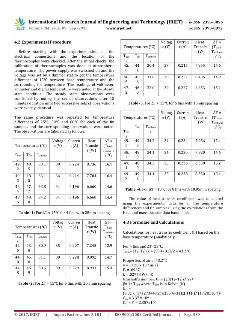
4.2 Experimental Procedure Before starting with the experimentation, all the electrical connections and the location of the thermocouples were checked. After the initial checks, the calibration of thermocouples was done at atmospheric temperature. The power supply was switched on and the voltage was set by a dimmer stat to get the temperature difference of 15°C between base temperature and the surrounding fin temperature. The readings of voltmeter, ammeter and digital temperature were noted at the steady state condition. The steady state observations were confirmed by noting the set of observations after 15 minutes duration until two successive sets of observations were exactly identical. The same procedure was repeated for temperature differences of 25°C, 50°C and 60°C for each of the fin samples and the corresponding observations were noted. The observations are tabulated as follows.

Temperatures (°C)

Voltage (V)

Current (A)

Heat Transfe

r (W)

∆T = (Tbase -

Tambient

) (°C) Tbas

e Tfin Tambien

t 49.2

48.5

33.1 39 0.224 8.736 16.1

49.5

48.5

33.1 36 0.214 7.704 16.4

48.4

47.7

33.8 34 0.196 6.660 14.6

48.6

48.0

34.2 34 0.196 6.660 14.4

Table -1: For ∆T ≈ 15°C for 4 fins with 28mm spacing

Temperatures (°C) Voltage (V)

Current (A)

Heat Transfe

r (W)

∆T = (Tbase -

Tambient

) (°C) Tbas

e Tfin Tambien

t 42.6

43.8

30.9 35 0.207 7.245 12.9

44.8

45.8

31.1 39 0.228 8.892 14.7

44.8

45.9

30.5 39 0.229 8.931 15.4

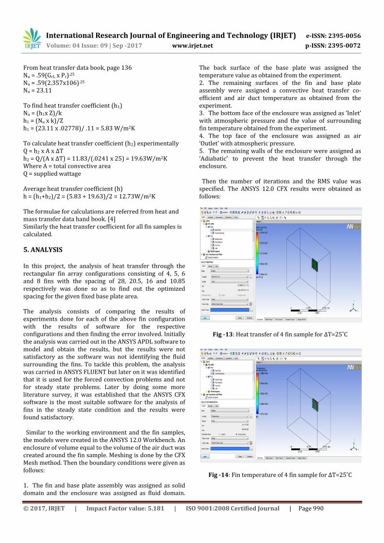
Table -2: For ∆T ≈ 15°C for 5 fins with 20.5mm spacing

Temperatures (°C)

Voltage (V)

Current (A)

Heat Transfe

r (W)

∆T = (Tbase -

Tambient

) (°C) Tbas

e Tfin Tambien

t 45.0

44.1

30.4 37 0.215 7.955 14.6

46.5

45.6

31.6 38 0.222 8.436 14.9

47.2

46.0

32.0 39 0.227 8.853 15.2

Table -3: For ∆T ≈ 15°C for 6 fins with 16mm spacing

Temperatures (°C) Voltage (V)

Current (A)

Heat Transfe

r (W)

∆T = (Tbase -

Tambient

) (°C) Tbas

e

Tfin Tambien

t

49.6

49.0

34.2 34 0.234 7.956 15.4

48.7

48.3

34.1 34 0.230 7.820 14.6

49.4

48.9

34.2 35 0.238 8.330 15.2

49.8

49.3

34.4 35 0.238 8.330 15.4

Table -4: For ∆T ≈ 15°C for 8 fins with 10.85mm spacing

The value of heat transfer co-efficient was calculated

using the experimental data for all the temperature differences and fin samples using the co-relations from the Heat and mass transfer data hand book.

4.3 Formulae and Calculations Calculations for heat transfer coefficient (h) based on the base temperature (Analytical): For 4 fins and ΔT=25°C, Tfilm= (T1+T3)/2 = (55.4+31)/2 = 43.2°C Properties of air at 43.2°C 𝜈 = 17.28 x 10-6 m2/s Pr = .6987 k = .02778 W/mK Grashoff’s number, GrL= (gβ(T1−T3)Z3)/ν2 β= 1/ Tfilm where Tfilm is in Kelvin (K) GrL = (9.81 x (1/ (273+43.2))x(55.4−31)x(.11)3)/ (17.28x10−6)2 GrL = 3.37 x 106 GrL x Pr = 2.357x106




From heat transfer data book, page 136 Nu = .59(GrL x Pr).25 Nu = .59(2.357x106).25 Nu = 23.11 To find heat transfer coefficient (h1) Nu = (h1x Z)/k h1 = (Nu x k)/Z h1 = (23.11 x .02778)/ .11 = 5.83 W/m2K To calculate heat transfer coefficient (h2) experimentally Q = h2 x A x ΔT h2 = Q/(A x ΔT) = 11.83/(.0241 x 25) = 19.63W/m2K Where A = total convective area Q = supplied wattage Average heat transfer coefficient (h) h = (h1+h2)/2 = (5.83 + 19.63)/2 = 12.73W/m2K The formulae for calculations are referred from heat and mass transfer data hand book. [4] Similarly the heat transfer coefficient for all fin samples is calculated.

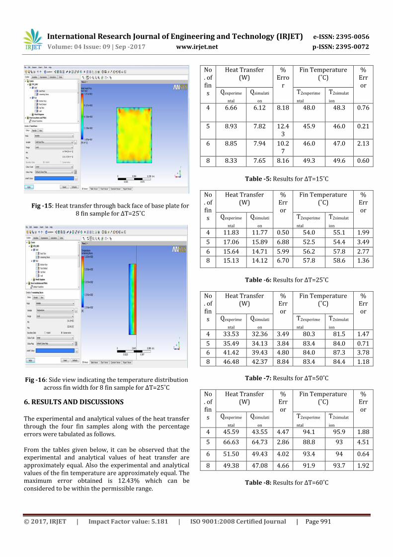
5. ANALYSIS In this project, the analysis of heat transfer through the rectangular fin array configurations consisting of 4, 5, 6 and 8 fins with the spacing of 28, 20.5, 16 and 10.85 respectively was done so as to find out the optimized spacing for the given fixed base plate area. The analysis consists of comparing the results of experiments done for each of the above fin configuration with the results of software for the respective configurations and then finding the error involved. Initially the analysis was carried out in the ANSYS APDL software to model and obtain the results, but the results were not satisfactory as the software was not identifying the fluid surrounding the fins. To tackle this problem, the analysis was carried in ANSYS FLUENT but later on it was identified that it is used for the forced convection problems and not for steady state problems. Later by doing some more literature survey, it was established that the ANSYS CFX software is the most suitable software for the analysis of fins in the steady state condition and the results were found satisfactory. Similar to the working environment and the fin samples, the models were created in the ANSYS 12.0 Workbench. An enclosure of volume equal to the volume of the air duct was created around the fin sample. Meshing is done by the CFX Mesh method. Then the boundary conditions were given as follows: 1. The fin and base plate assembly was assigned as solid domain and the enclosure was assigned as fluid domain.

The back surface of the base plate was assigned the temperature value as obtained from the experiment. 2. The remaining surfaces of the fin and base plate assembly were assigned a convective heat transfer co-efficient and air duct temperature as obtained from the experiment. 3. The bottom face of the enclosure was assigned as ‘Inlet’ with atmospheric pressure and the value of surrounding fin temperature obtained from the experiment. 4. The top face of the enclosure was assigned as air ‘Outlet’ with atmospheric pressure. 5. The remaining walls of the enclosure were assigned as ‘Adiabatic’ to prevent the heat transfer through the enclosure. Then the number of iterations and the RMS value was specified. The ANSYS 12.0 CFX results were obtained as follows:

Fig -13: Heat transfer of 4 fin sample for ΔT=25˚C

Fig -14: Fin temperature of 4 fin sample for ΔT=25˚C




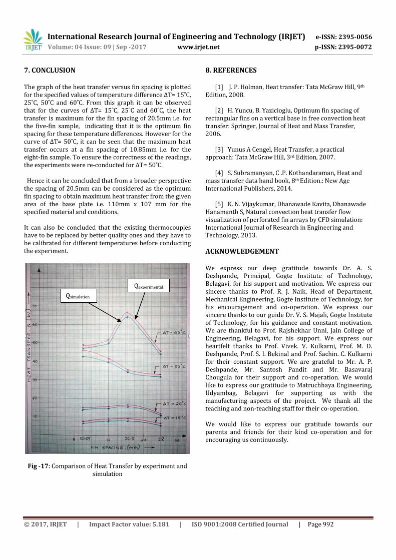
Fig -15: Heat transfer through back face of base plate for 8 fin sample for ΔT=25˚C

Fig -16: Side view indicating the temperature distribution across fin width for 8 fin sample for ΔT=25˚C

6. RESULTS AND DISCUSSIONS The experimental and analytical values of the heat transfer through the four fin samples along with the percentage errors were tabulated as follows. From the tables given below, it can be observed that the experimental and analytical values of heat transfer are approximately equal. Also the experimental and analytical values of the fin temperature are approximately equal. The maximum error obtained is 12.43% which can be considered to be within the permissible range.

No. of fins

Heat Transfer (W)

% Erro

r

Fin Temperature (˚C)

% Error

Qexperime

ntal Qsimulati

on T2experime

ntal T2simulat

ion 4 6.66 6.12 8.18 48.0 48.3 0.76

5 8.93 7.82 12.43

45.9 46.0 0.21

6 8.85 7.94 10.27

46.0 47.0 2.13

8 8.33 7.65 8.16 49.3 49.6 0.60

Table -5: Results for ΔT=15˚C

No. of fins

Heat Transfer (W)

% Error


% Error

Qexperime

ntal Qsimulati

on T2experime

ntal T2simulat

ion 4 11.83 11.77 0.50 54.0 55.1 1.99

5 17.06 15.89 6.88 52.5 54.4 3.49

6 15.64 14.71 5.99 56.2 57.8 2.77

8 15.13 14.12 6.70 57.8 58.6 1.36


No. of fins

Heat Transfer (W)

% Error


% Error

Qexperime

ntal Qsimulati

on T2experime

ntal T2simulat

ion 4 33.53 32.36 3.49 80.3 81.5 1.47

5 35.49 34.13 3.84 83.4 84.0 0.71

6 41.42 39.43 4.80 84.0 87.3 3.78

8 46.48 42.37 8.84 83.4 84.4 1.18


No. of fins

Heat Transfer (W)

% Error


% Error

Qexperime

ntal Qsimulati

on T2experime

ntal T2simulat

ion 4 45.59 43.55 4.47 94.1 95.9 1.88

5 66.63 64.73 2.86 88.8 93 4.51

6 51.50 49.43 4.02 93.4 94 0.64

8 49.38 47.08 4.66 91.9 93.7 1.92





7. CONCLUSION The graph of the heat transfer versus fin spacing is plotted for the specified values of temperature difference ΔT= 15˚C, 25˚C, 50˚C and 60˚C. From this graph it can be observed that for the curves of ΔT= 15˚C, 25˚C and 60˚C, the heat transfer is maximum for the fin spacing of 20.5mm i.e. for the five-fin sample, indicating that it is the optimum fin spacing for these temperature differences. However for the curve of ΔT= 50˚C, it can be seen that the maximum heat transfer occurs at a fin spacing of 10.85mm i.e. for the eight-fin sample. To ensure the correctness of the readings, the experiments were re-conducted for ΔT= 50˚C. Hence it can be concluded that from a broader perspective the spacing of 20.5mm can be considered as the optimum fin spacing to obtain maximum heat transfer from the given area of the base plate i.e. 110mm x 107 mm for the specified material and conditions. It can also be concluded that the existing thermocouples have to be replaced by better quality ones and they have to be calibrated for different temperatures before conducting the experiment.

Fig -17: Comparison of Heat Transfer by experiment and simulation

8. REFERENCES

[1] J. P. Holman, Heat transfer: Tata McGraw Hill, 9th Edition, 2008.

[2] H. Yuncu, B. Yazicioglu, Optimum fin spacing of

rectangular fins on a vertical base in free convection heat transfer: Springer, Journal of Heat and Mass Transfer, 2006.

[3] Yunus A Cengel, Heat Transfer, a practical

approach: Tata McGraw Hill, 3rd Edition, 2007. [4] S. Subramanyan, C .P. Kothandaraman, Heat and

mass transfer data hand book, 8th Edition.: New Age International Publishers, 2014.

[5] K. N. Vijaykumar, Dhanawade Kavita, Dhanawade

Hanamanth S, Natural convection heat transfer flow visualization of perforated fin arrays by CFD simulation: International Journal of Research in Engineering and Technology, 2013.

ACKNOWLEDGEMENT We express our deep gratitude towards Dr. A. S. Deshpande, Principal, Gogte Institute of Technology, Belagavi, for his support and motivation. We express our sincere thanks to Prof. R. J. Naik, Head of Department, Mechanical Engineering, Gogte Institute of Technology, for his encouragement and co-operation. We express our sincere thanks to our guide Dr. V. S. Majali, Gogte Institute of Technology, for his guidance and constant motivation. We are thankful to Prof. Rajshekhar Unni, Jain College of Engineering, Belagavi, for his support. We express our heartfelt thanks to Prof. Vivek. V. Kulkarni, Prof. M. D. Deshpande, Prof. S. I. Bekinal and Prof. Sachin. C. Kulkarni for their constant support. We are grateful to Mr. A. P. Deshpande, Mr. Santosh Pandit and Mr. Basavaraj Chougula for their support and co-operation. We would like to express our gratitude to Matruchhaya Engineering, Udyambag, Belagavi for supporting us with the manufacturing aspects of the project. We thank all the teaching and non-teaching staff for their co-operation. We would like to express our gratitude towards our parents and friends for their kind co-operation and for encouraging us continuously.

Qexperimental

Qsimulation




BIOGRAPHIES

Name: Aditya Yardi Achievements: Secured 1st place in National Level Technical Fest ‘Paanchajanya’ 2012 Quiz Competition. Secured 1st place in National Level Technical Fest ‘Avalanche’ 2015 Paper Presentation. Bagged 2nd place in Technical Fest ‘Invento’ 2015 Paper presentation.

Name: Ashish Karguppikar Achievements: Co-ordinated and participated in a one week workshop on ‘Micro-controller and Embedded Programming’ conducted by Advanced Electronic Systems in KLS’s Gogte Institute of technology. Represented South zone in ‘Vidyabharathi’ National Level Handball Tournament held at Gwalior in 2009-2010. Attended a basic industrial training at AKP Foundries (Training Period: 10 days). Name: Gourav Tanksale Achievements: Attended training for software’s like Catia V5 and AutoCAD 10. Participated in technical fests in college in competitions like Quiz, Simplex to Complex, etc.

Name: Kuldeepak Sharma Achievements: Participated in ‘Technophilia Workshop on Haptic robotic arm’ in KLS’s Gogte Institute of Technology. Bagged 2nd place in Robo-wars competition in Technical fest in KLS’s Gogte Institute of Technology. Actively participated in cultural activities and social welfare activities.

Documents

Optimization of Fin spacing by analyzing the heat transfer ...For a fixed temperature difference between the base plate and the air duct temperature, the heat transfer values were