Embed Size (px)
Citation preview
64 Amity Journal of Operations ManagementADMAA
Volume 1 Issue 1 2016AJOM
Amity Journal of Operations Management1(1), (64-76)
©2016 ADMAA
Optimization of Deteriorating Items Inventory Model with Price and Time Dependent Demand
Shiv Kumar Indian School of Mines, Dhanbad, Jharkhand, India
(Received: 14/12/2015; Accepted: 26/04/2016)
AbstractThe study of deteriorating items-inventory system has been drawing more interest since it influences
the cost of a retailer. In any organization, consumer’s rate of demand depends upon selling price as well as it depends also on deteriorating items of the product. There are many causes of deteriorating items of the product such as time, selling price, stock level of items, capacity of warehouse, quality and quantity, consumer’s needs of the product etc. The study have developed an inventory model with price and time dependent demand of deteriorating items where deterioration rate may be considered as variable or constant type. With the help of numerical example, optimum profit function has been illustrated. Sensitivity analysis has also been derived to study the effect of the parameters connected with the proposed model.
Keywords: Time and Price Dependent Demand, Deteriorating Items Inventory
JEL Classification: C61, E22
Paper Classification: Research Paper
IntroductionIn the real life situation, it is quite difficult to maintain the deteriorating items inventory. The
deteriorating item has a significant impact on the cost of the system. Normally the products are stored the product for present or future use but due to deterioration, fraction amount of product is decayed or spoilt, and cannot satisfy the future demand. The loss due to deterioration cannot be neglected. Due to deterioration, inventory system faces the crisis of shortages and loss of profit. Shortage is a fraction of those customers whose demand is not satisfied in the current period. During shortage period, the demand is either backlogged or lost. Therefore it is very important to discuss the deteriorating behaviour of such type of inventory.
Literature ReviewClassical deterministic inventory models considered the demand rate to be either stock
dependent or constant or time dependent. It has been observed that decrease in price of the
65Amity Journal of Operations Management
Volume 1 Issue 1 2016 AJOM
ADMAA
product generally has a positive effect on demand of the product. It becomes a necessity to make a proper strategy to maintain the inventory economically. Ghare and Schrader (1963) describe the optimal ordering policy for exponentially decaying inventory.
Deb and Chaudhari (1986) explained inventory model with time dependent deterioration rate. Jie, Zhou, and Zhao (2010) have established a deteriorating inventory model considering stock dependent demand. Mandol, Dey, and Maiti (2007) worked on a single period inventory model of deteriorating product in which they considered that demand is function of time only. Kaur and Sharma (2012) have established an inventory model for deteriorating item with price and time dependent demand but they assumed that the rate of deterioration is constant. However, constant deterioration is the feature of static environment, while now-a-days, for such a dynamic atmosphere nothing is constant or fixed. Kumar and Singh (2015) derived an inventory model, consumer’s demand in the super market is not only depend upon stock of inventory level but it also depends upon selling price of items.
Research Gap & Contribution of StudyThe present model has been developed considering the demand rate as a function which is
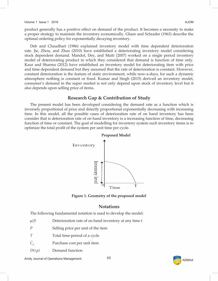
inversely proportional of price and directly proportional exponentially decreasing with increasing time. In this model, all the possible cases of deterioration rate of on hand inventory has been consider that is deterioration rate of on hand inventory is a increasing function of time, decreasing function of time or constant. The goal of modelling for inventory system such inventory items is to optimize the total profit of the system per unit time per cycle.
Proposed Model
Figure 1. Geometry of the proposed model
NotationsThe following fundamental notation is used to develop the model:
m(f) Deterioration rate of on hand inventory at any time t
P Selling price per unit of the item
T Total time-period of a cycle
CP Purchase cost per unit item
D(t,p) Demand function

66 Amity Journal of Operations ManagementADMAA
Volume 1 Issue 1 2016AJOM
A Ordering cost per cycle per unit time
I(t) Inventory level at any time t
Ch Holding cost per unit per unit time
l Any constant number
b Any constant number
Cd Deterioration cost per unit item
PF* Optimal profit per unit time per cycle
Z (t) Stock loss at any time t
Z Total stock loss per cycle
Assumptions1: The deterioration rate of on hand inventory at time t is considered as
1, where 0< <1 ( ) ( )tt tblm m−=
=1; µ(t) is constant . 1; µ(t) is increasing function with t . 1; µ(t) is decreasing function with t.
for bb
b>
<
2. The demand function D(t,p) is exponentially decreasing with time and inversely decreasing with the selling price p and is expressed as
( , ) ,
teD t p
p
q−=
Where q is a constant.
3. Lead time is zero.
4. Shortages are not permitted.
Mathematical AnalysisIn interval [0,T], the inventory level reduces due to deterioration and demand. If I(t) be the on
hand inventory at t ≥ 0, then at time t + ∆ t, the inventory level in the interval [0, T ] will be
( ) ( ) ( ) ( ) - ( , )I t t I t µ t I t t D p t t+ ∆ = − ∆ ∆
Where the deteriorating rate 1( ) : 0< ( )<1 t t tbm l m−= and the demand function
( , )teD t p p
q−=
Dividing by ∆ t and then taking limit as ∆ t → 0
67Amity Journal of Operations Management
Volume 1 Issue 1 2016 AJOM
ADMAA
( ) ( ) ( ) - ( , )dI t µ t I t D t pdt
+ = (1)
With initial condition
( ) 0 ( ) (0) 0 I T at t T and I t I at t= = = = (2)
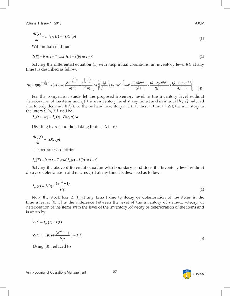
Solving the differential equation (1) with help initial conditions, an inventory level I(t) at any time t is described as follow:
( ) ( )1 1 2 1 2 1 2 2 1
1 1 2 2 ( 2) ( 1)( ) (0) ( ) 1 1( ) ( ) 1 ( 1) 2( 1) 2( 1)
t tt e e t t tI t I e d p t t
d p d p
b bb
l ll b b b b b
b bq lb lbq b lq b l qq qb b b b
− − + + − + − − + −
+ += + − + + − + + + + + + + + (3)
For the comparison study let the proposed inventory level, is the inventory level without deterioration of the items and Iw(t) is an inventory level at any time t and in interval [0, T] reduced due to only demand. If Iw(t) be the on hand inventory at t ≥ 0, then at time t + ∆ t, the inventory in the interval [0, T ] will be
( ) ( ) - ( , )w wI t t I t D t p t+ ∆ = ∆
Dividing by ∆ t and then taking limit as ∆ t →0
( )- ( , )wdI tD t p
dt=
The boundary condition
( ) 0 ( ) (0) 0 w wI T at t T and I t I at t= = = =
Solving the above differential equation with boundary conditions the inventory level without decay or deterioration of the items Iw(t) at any time t is described as follow:
( 1)( ) (0) t
WeI t I
p
q
q
− −= +
(4)
Now the stock loss Z (t) at any time t due to decay or deterioration of the items in the time interval [0, T] is the difference between the level of the inventory of without –decay, or deterioration of the items with the level of the inventory ,of decay or deterioration of the items and is given by
( ) ( ) ( ) WZ t I t I t= −
( 1)( ) { (0) } ( ) teZ t I I tp
q
q
− −= + −
(5)
Using (3), reduced to

68 Amity Journal of Operations ManagementADMAA
Volume 1 Issue 1 2016AJOM
( )
( )
11
1 2 1 2 1 2 2 11 2
( 1)( ) { (0) } (0) ( ) 1( )
2 ( 2) ( 1) 1( ) 1 ( 1) 2( 1) 2( 1)
tt
t
te eZ t I I e d pp d p
e t t tt td p
bb
b
ll b
b
lb b b b
b
q qq
lb lbq b lq b l qq qb b b b
− + − +
− + − + −
−
− −= + − + − +
+ +
+ − + + + + + + + + (6)
Total demand during the time interval (0,T) is given by
0
( , ) dt
( 1)
T t
T
eD t pp
ep
q
q
q
−
−
=
−= −
∫
(7)
Total stock lost for the duration of the time interval is given by
{ } ( )
( )
1 1
0 0 0 0
12 1 2 11 11 2
0
11( ) (0) 1 1
1 2 ( 2)11 ( 1)
t tT T T T
tT t t
tep
Z Z t dt I e dt dt e dtp p
t e t ete t ep
b b
bb b
l lb b
l ll l b bb b
b bb
q qq
lb lbq b lqq qb b
− − + +
− − +− + − − + +−
− − = = − + − +
+ − + − + + + + +
∫ ∫ ∫ ∫
∫1
12 2 1
2( 1)
( 1) 2( 1)
t
tt e dt
b
blbb
b
b l qb
+
− +−
+
+
+ +
2 11 2
2 2 1
2 2 2 32 2 2
2 2 3
2 1 22
1 1 ( 1)(0) ( )2 1( 1)
1 1 (1 ) T T 1 + T- ( ) - ( )p ( 1)( 2) 2 1 ( 1) ( 1) 2 2 1
1 T- ( )2 1( 1)
TT eZ I T Tp
T TT
TT
b qb
b
b b b bb
b b
b
l lb q qb
l l lb q l lb b b b b b b b
l lqbb
+ −+
+
++
+
+
−= − + − ++
−+ + + + + + + + +
+++
2 1 2 2 3 42
2 1 4
2 2 3 2 2 12( 1) 2 1 2
2 3 2 2 2 1
2 T T 1- ( )( 1) 2 2 ( 1) 3 2 1
( 2) T 1 ( 1) 1 + - T ( ) T- ( )2( 1) ( 2) 2 1 2 12( 1) ( 1)
T
T p TTp
b b b b
b b
b b bb b
b b
lbq l q l lb b b b b
l b q l l q l lb b b bb b
+
+
+ + ++ +
+ +
+ + +
+ + + + −
+ + + + + + ++ + (8)
Lot size QT= Total demand+ Total deteriorated item

69Amity Journal of Operations Management
Volume 1 Issue 1 2016 AJOM
ADMAA
2 11 2
2 2 1
2 2 2 32 2 2
2 2 3
( , ) ( )
( 1) 1 1 ( 1)(0) ( )( 1) 2 1
1 1 (1 ) T T 1 T- ( ) - ( )p ( 1)( 2) 2 1 ( 1) ( 1) 2 2 1
T
t T
T
Q D p t Z T
e T eQ I T Tp p
T TT
q b qb
b
b b b bb
b b
l lq b b q q
l l lb q l lb b b b b b b b
− + −+
+
++
+
= +
− −= − + − + − + +
−+ + + + + + + + +
2 1 2 2 3 42 1 2 2
2 2 1 4
2 2 3 22( 1) 2 1
2 3 2 2
1 2 T T 1+ T- ( ) - ( )( 1) 2 1 ( 1) 2 2 ( 1) 3 2 1
( 2) T 1 ( 1) 1 + - T ( ) T- (2( 1) ( 2) 2( 1) 2 1 ( 1) 2
T TT
T p Tp
b b b bb
b b
b bb b
b
l l lbq l q l lqb b b b b b b
l b q l l q l lb b b b b b
++
+
+ ++ +
+
+ + + + + + + + +
+ −+ + + + + + + +
2 12
2 1)1
T b
b
+
+
+
(9)
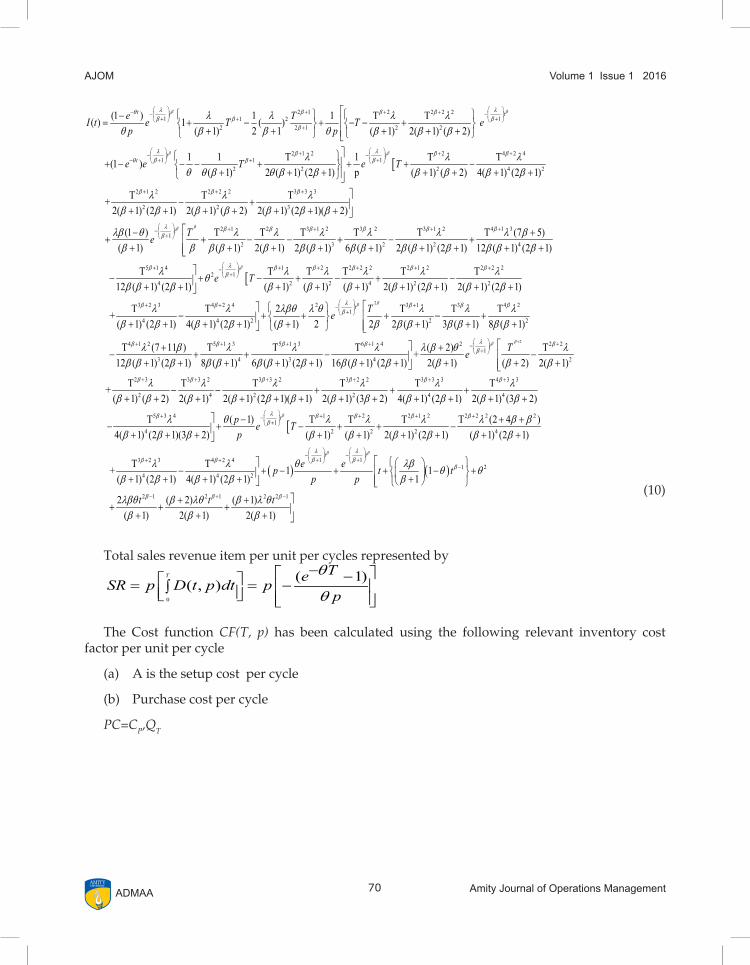
The Lot size QT is the starting on hand inventory or the inventory at time t=0 that is I(0) hence I(0)=QT therefore on hand inventory at any time I(t) can be derived using (9) as:
[
2 1 2 2 2 21 2
2 2 1 2 2
2 1 2 2 4 2 41
2 2 2 4
(1 ) 1 1 T T(0) 1 ( ) 2 1( 1) ( 1) 2( 1) ( 2)
1 1 T 1 T T (1 )p( 1) 2 ( 1) (2 1) ( 1) ( 2) 4( 1) (2 1
t
t
e TI T Tp p
e T T
q b b bb
b
b b bq b
l l l lq b qb b b b
l l lq q b q b b b b b b
− + + ++
+
+ + +− +
−= + − + − − + ++ + + +
+ − − − + + + − + + + + + + +
2
2 1 2 2 2 2 3 3 3
2 2 3
2 1 2 3 1 2 3 2 3 1 2 4 1 3
2 3 2 2
)
T T T +2( 1) (2 1) 2( 1) ( 2) 2( 1) (2 1)( 2)
(1 ) T T T T T T (7 5) ( 1) 2( 1)( 1) 2 ( 1) 6 ( 1) 2 ( 1) (2 1) 12
Tb
b b b
b b b b b b
l l lb b b b b b b
lb q l l l l l l bb b bb b b b b b b b b b
+ + +
+ + + +
− + + + + + + + +
− ++ + − − + − +
+ ++ + + + +
[
4
5 1 4 1 2 2 2 2 2 1 2 2 2 22
4 2 2 4 2 2
3 2 3 4 2 4 2
4 4 2
( 1) (2 1)
T T T T T T 12 ( 1) (2 1) ( 1) ( 1) ( 1) 2( 1) (2 1) 2( 1) (2 1)
T T 2 +( 1) 2( 1) (2 1) 4( 1) (2 1)
Tb b b b b b
b b
b b
l l l l l lqb b b b b b b b b b
l l lbq l qbb b b b
+ + + + + +
+ +
+ +
− + − + − + −+ + + + + + + + +
− + + ++ + + +
2
2
3 1 3 4 2
2 2
4 1 2 5 1 3 5 1 3 6 1 4 2 2 2
3 4 3 4
T T T2 3 ( 1)2 ( 1) 8 ( 1)
T (7 11 ) T T T ( 2) T +2( 1) ( 2)12 ( 1) (2 1) 8 ( 1) 6 ( 1) (2 1) 16 ( 1) (2 1) 2( 1)
T
T
b
b
b b b
b b b b b
l l lb b bb b b b
l b l l l l b q lb bb b b b b b b b b b b b
+
+
+ + + + +
+ − +
++ + + +
− + + − − + ++ + + + + + + +
[
2
2 3 3 3 2 3 3 2 3 2 2 3 3 3 4 3 3
2 4 2 2 4 4
5 3 4 1 2
4 2
T T T T T T +( 1) ( 2) 2( 1) 2( 1) (2 1)( 1) 2( 1) (3 2) 4( 1) (2 1) 2( 1) (3 2)
T ( 1) T T 4( 1) (2 1)(3 2) ( 1) ( 1
p Tp
b b b b b b
b b b
l l l l l lb b b b b b b b b b b b
l q l lb b b b b
+ + + + + +
+ + +
− − + + ++ + + + + + + + + + + +
−− + − ++ + + + +
2 1 2 2 2 2 2
2 2 4
3 2 3 4 2 4
4 4 2
T T (2 4 )) 2( 1) (2 1) ( 1) (2 1)
T T +( 1) (2 1) 4( 1) (2 1)
b b
b b
l l b bb b b b
l lb b b b
+ +
+ +
+ ++ −
+ + + +
− + + + +
70 Amity Journal of Operations ManagementADMAA
Volume 1 Issue 1 2016AJOM
2 1 2 2 2 21 11 2
2 2 1 2 2
2 1 21 1
2 2
(1 ) 1 1 T T( ) 1 ( ) 2 1( 1) ( 1) 2( 1) ( 2)
1 1 T (1 )( 1) 2 ( 1) (2 1)
t t t
tt
e TI t e T T ep p
e e T
b b
b
l lq b b bb bb
b
l bbq b
l l l lq b qb b b b
lq q b q b b
− + + +− − + ++ +
+− +− +
− = + − + − − + ++ + + +
+ − − − +
+ + +[
2 4 2 41
2 4 2
2 1 2 2 2 2 3 3 3
2 2 3
2 11
2
1 T Tp ( 1) ( 2) 4( 1) (2 1)
T T T +2( 1) (2 1) 2( 1) ( 2) 2( 1) (2 1)( 2)
(1 ) T T ( 1) ( 1)
t
t
e T
Te
b
bb
l b bb
b b b
l bb
l lb b b b
l l lb b b b b b b
lb q lb b b b
+ +− +
+ + +
+− +
+ + −
+ + + +
− + + + + + + + +
−+ + −
+ +
[
2 3 1 2 3 2 3 1 2 4 1 3
3 2 2 4
5 1 4 1 2 2 2 2 2 1 212
4 2 2 4 2
T T T T (7 5)2( 1) 2 ( 1) 6 ( 1) 2 ( 1) (2 1) 12 ( 1) (2 1)
T T T T T 12 ( 1) (2 1) ( 1) ( 1) ( 1) 2( 1) (2
te T
b
b b b b b
lb b b b bb
l l l l l bb b b b b b b b b b b
l l l l lqb b b b b b b b
+ + +
+ + + + +− +
+− + − +
+ + + + + + +
− + − + − ++ + + + + + +
2
2 2 2
2
3 2 3 4 2 4 2 3 1 3 4 21
4 4 2 2 2
4 1 2
3
T1) 2( 1) (2 1)
T T 2 T T T +( 1) 2 2 3 ( 1)( 1) (2 1) 4( 1) (2 1) 2 ( 1) 8 ( 1)
T (7 11 ) 12 ( 1) (2 1
t Tebb
b
lb b b b bb
b
lb b
l l lbq l q l l lb b b bb b b b b b b b
l bb b b
+
+ + +− +
+
−+ +
− + + + − + + ++ + + + + +
+−
+ +
25 1 3 5 1 3 6 1 4 2 2 21
4 3 4 2
2 3 3 3 2 3 3 2 3 2 2
2 4 2
T T T ( 2) T+2( 1) ( 2)) 8 ( 1) 6 ( 1) (2 1) 16 ( 1) (2 1) 2( 1)
T T T T +( 1) ( 2) 2( 1) 2( 1) (2 1)( 1) 2(
t Tebblb b b b
b
b b b b
l l l l b q lb bb b b b b b b b b
l l l lb b b b b b b
+ + + + +− +
+ + + +
++ + − − + ++ + + + + +
− − ++ + + + + + +
[
3 3 3 4 3 3
2 4 4
5 3 4 1 2 2 1 2 2 2 2 21
4 2 2 2 4
3
T T1) (3 2) 4( 1) (2 1) 2( 1) (3 2)
T ( 1) T T T T (2 4 ) 4( 1) (2 1)(3 2) ( 1) ( 1) 2( 1) (2 1) ( 1) (2 1)
T +
tp e Tp
b
b b
lb b b b bb
b
l lb b b b b
l q l l l l b bb b b b b b b b b
+ +
+ + + + +− +
+
+ ++ + + + +
− + +− + − + + −+ + + + + + + + +
( ) ( )1 12 3 4 2 4
1 24 4 2
2 1 2 1 2 2 1
T 1 1 1( 1) (2 1) 4( 1) (2 1)
2 ( 2) ( 1) ( 1) 2( 1) 2( 1)
t te ep t t
p p
t t t
b bl lb bb
b
b b b
l l q lb q qbb b b b
lbq b lq b l qb b b
− − + ++
−
− + −
− + − + + − + ++ + + +
+ ++ + + + + +
(10)
Total sales revenue item per unit per cycles represented by
0
( 1)( , )T TeSR p D t p dt p
p
q
q
− − = = − ∫
The Cost function CF(T, p) has been calculated using the following relevant inventory cost factor per unit per cycle
(a) A is the setup cost per cycle
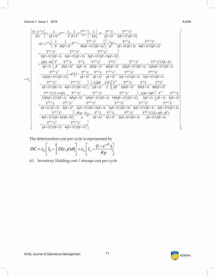
(b) Purchase cost per cycle
PC=CP,QT
71Amity Journal of Operations Management
Volume 1 Issue 1 2016 AJOM
ADMAA
[
2 1 2 2 2 21 2
2 2 1 2 2
2 1 2 2 4 2 41
2 2 2 4 2
(1 ) 1 1 T T1 ( ) 2 1( 1) ( 1) 2( 1) ( 2)
1 1 T 1 T T (1 )p( 1) 2 ( 1) (2 1) ( 1) ( 2) 4( 1) (2 1)
t
t
p
e TT Tp p
e T T
C
q b b bb
b
b b bq b
l l l lq b qb b b b
l l lq q b q b b b b b b
− + + ++
+
+ + +− +
−+ − + − − + ++ + + +
+ − − − + + + − + + + + + + +
=
2 1 2 2 2 2 3 3 3
2 2 3
2 1 2 3 1 2 3 2 3 1 2 4 1 3
2 3 2 2
T T T +2( 1) (2 1) 2( 1) ( 2) 2( 1) (2 1)( 2)
(1 ) T T T T T T (7 5) ( 1) 2( 1)( 1) 2 ( 1) 6 ( 1) 2 ( 1) (2 1) 12 (
Tb
b b b
b b b b b b
l l lb b b b b b b
lb q l l l l l l bb b bb b b b b b b b b b b
+ + +
+ + + +
− + + + + + + + +
− ++ + − − + − +
+ ++ + + + +
[
4
5 1 4 1 2 2 2 2 2 1 2 2 2 22
4 2 2 4 2 2
3 2 3 4 2 4 2
4 4 2
1) (2 1)
T T T T T T 12 ( 1) (2 1) ( 1) ( 1) ( 1) 2( 1) (2 1) 2( 1) (2 1)
T T 2 +( 1) 2( 1) (2 1) 4( 1) (2 1)
Tb b b b b b
b b
b
l l l l l lqb b b b b b b b b b
l l lbq l qbb b b b
+ + + + + +
+ +
+ +
− + − + − + −+ + + + + + + + +
− + + ++ + + +
2
2
3 1 3 4 2
2 2
4 1 2 5 1 3 5 1 3 6 1 4 2 2 2
3 4 3 4 2
T T T2 3 ( 1)2 ( 1) 8 ( 1)
T (7 11 ) T T T ( 2) T +2( 1) ( 2)12 ( 1) (2 1) 8 ( 1) 6 ( 1) (2 1) 16 ( 1) (2 1) 2( 1)
T
T
b
b
b b b
b b b b b
l l lb b bb b b b
l b l l l l b q lb bb b b b b b b b b b b b
+
+
+ + + + +
+ − +
++ + + +
− + + − − + ++ + + + + + + +
[
2 3 3 3 2 3 3 2 3 2 2 3 3 3 4 3 3
2 4 2 2 4 4
5 3 4 1 2
4 2 2
T T T T T T +( 1) ( 2) 2( 1) 2( 1) (2 1)( 1) 2( 1) (3 2) 4( 1) (2 1) 2( 1) (3 2)
T ( 1) T T 4( 1) (2 1)(3 2) ( 1) ( 1)
p Tp
b b b b b b
b b b
l l l l l lb b b b b b b b b b b b
l q l lb b b b b
+ + + + + +
+ + +
− − + + ++ + + + + + + + + + + +
−− + − ++ + + + +
2 1 2 2 2 2 2
2 4
3 2 3 4 2 4
4 4 2
T T (2 4 )2( 1) (2 1) ( 1) (2 1)
T T +( 1) (2 1) 4( 1) (2 1)
b b
b b
l l b bb b b b
l lb b b b
+ +
+ +
+ +
+ − + + + + − + + + +
The deterioration cost per cycle is represented by
1
00
(1 )( , )T
d d o
t eDC c I D t p dt c Ip
q
q
− −= − = −∫
(c) Inventory Holding cost / storage cost per cycle

72 Amity Journal of Operations ManagementADMAA
Volume 1 Issue 1 2016AJOM
( )0
2 3 2 2 2 2 2 2 2 2 3 2 11 2
2 3 2 2 2 1
2 2
2
( )
1 1 T T T (1 ) T T 11 1 ( )( 1)( 2) 2( 3) 2 12( 1) (2 1) 4( 1) 4( 1) (2 3) ( 1)
1 T T( 1)
=
T
T
HC ch I t dt
TT e Tp
Tp
ch
b b b b b bq b
b
b b
lq lq l l l l l lq q b b b bb b b b b b
lq b
+ + + + + +− +
+
+ +
= ∫
−+ − − + + + − + − +
+ + + ++ + + + + +
− − ++
( )
2 2 1 2 12
2 2 2 1
2 3 2 2 2 2 2 2 2 2 3
2 3 2
12
T 1 ( ) 2 12( 1) ( 2) ( 1)
1 T T T (1 ) T T1( 1)( 2) 2( 3) 2( 1) (2 1) 4( 1) 4( 1) (2 3)
1 1
( 1)
T
TT
T e
T
b b
b
b b b b bq
b
l l lbb b b
lq lq l l l lq b b b b b b b b
q q b
+ +
+
+ + + + +−
+
− + ++ + +
−+ + − − + + + −
+ + + + + + + +
− −+
[
2 1 2
2
1 2 1 2 4 2 42
2 2 1 2 4 2
2 1 2 2 2 2 3 3 3
2 2 3
T2 ( 1) (2 1)
1 T 1 T T( )p 2 1( 1) ( 1) ( 2) 4( 1) (2 1)
T T T +2( 1) (2 1) 2( 1) ( 2) 2( 1) (2 1)( 2)
TT T
b
b b b b
b
b b b
lq b b
l l l lbb b b b b
l l lb b b b b b b
+
+ + + +
+
+ + +
+ + +
+ − + + −
++ + + + +
− + + + + + + + + 1 2 1 2 1 2 3 1 2
22 2 1 2 3
3 2 3 1 2 4 1 3 5 1 4
2 2 4 4
12
(1 ) T 1 T T T( )( 1) 2 1 2( 1)( 1) ( 1) 2 ( 1)
T T T (7 5) T6 ( 1) 2 ( 1) (2 1) 12 ( 1) (2 1) 12 ( 1) (2 1)
T
T TT
T
bb b b b b
b
b b b b
b
lb q l l l l lb b b bb b b b b
l l l b lb b b b b b b b b b b
lq
+ + + +
+
+ + +
+
−+ − + + − − +
+ + ++ + + +
− + − + + + + + + +
+ − [2 1 1 2 2 2 2 2 1 2 2 2 2
22 2 1 2 2 4 2 2
3 2 3 4 2 4 2 1
4 4 2 2
1 T T T T T( )2 1( 1) ( 1) ( 1) ( 1) 2( 1) (2 1) 2( 1) (2 1)
T T 2 T +( 1) 2( 1) (2 1) 4( 1) (2 1) ( 1)
T T
T
b b b b b b
b
b b b
l l l l l lbb b b b b b b b
l l lbq l q lbb b b b b
+ + + + + +
+
+ + +
+ − + − + −
++ + + + + + + +
− + + − ++ + + + + 2
2 12
2 1
3 1 3 4 2
2 2
4 1 2 5 1 3 5 1 3 6 1 4 2 1
3 4 3 4
1 ( )2 1
T T T2 3 ( 1)2 ( 1) 8 ( 1)
T (7 11 ) T T T ( 2) T +2( 1)12 ( 1) (2 1) 8 ( 1) 6 ( 1) (2 1) 16 ( 1) (2 1)
T
T
T
b
b
b
b b b
b b b b b
lb
l l lb b bb b b b
l b l l l l b q lbb b b b b b b b b b b
+
+
+
+ + + + +
+
+
+ − +++ +
+ +− + + − − ++ + + + + + + 2
2 12
2 2 1
2 2 2 3 3 3 2 3 3 2 3 2 2 3 3 3 4 3 3
2 2 4 2 2 4 4
5 3 4
1 ( )2 1( 1)
T T T T T T T+( 2) 2( 1) ( 1) ( 2) 2( 1) 2( 1) (2 1)( 1) 2( 1) (3 2) 4( 1) (2 1) 2( 1) (3 2)
T 4(
T
Tb
b
b
b b b b b b b
b
lbb
l l l l l l lb b b b b b b b b b b b b b
lb
+
+
+
+ + + + + + +
+
+
++
− − − + + ++ + + + + + + + + + + + + +
−+
]
1 2 12
4 2 2 1
1 2 2 1 2 2 2 2 2 3 2 3 4 2 4
2 2 2 4 4 4 2
( 1) T 1 ( )2 11) (2 1)(3 2) ( 1)
T T T T (2 4 ) T T+ 1( 1) ( 1) 2( 1) (2 1) ( 1) (2 1) ( 1) (2 1) 4( 1) (2 1)
p TTp
T
b b
b
b b b b b b
q l lbb b b
l l l l b b l lb b b b b b b b b b
+ +
+
+ + + + + +
−+ − + ++ + +
+ + − + + − − + + + + + + + + + + +
( )2 2 2 2 2 2 2 3 2
3 2 2
1 2 1 2 2 2 22 2
2 2 1 2
T T T T1 1 2 ( 1)( 2) 14( 1) 2( 1) 6 ( 1)
T 1 ( 2) T T ( )2 1 2( 1) 2( 1) 2( 1)
T T
p
T TT
b b b b b
b b b b
b
l l lb l lq
b b b bb b b b
l l b lq lq
b b bb b
+ + +
+ + + +
+
− + + − − + + + + + ++ + +
+− + + − +
+ + ++ +
3 2 2
2
2 2 3 2 4 2
2
2 ( 1) (3 2)
2 ( 1) T T( 1) 2( 1) 2 2( 1)(3 2) 8 ( 1)
T
b
b b b
lb b b
lbq b l q l lb b b b b b b
+
+
+ + ++ + − + + + + + +
Total cost of the system per cycle is given by
( ) Setup cost Inventory holding/storage cost Deterioration cost Purchase cost
, A HCCF T pDC PC
+ +=+
Or ( ),CF T p A HC DC PC = + + +
73Amity Journal of Operations Management
Volume 1 Issue 1 2016 AJOM
ADMAA
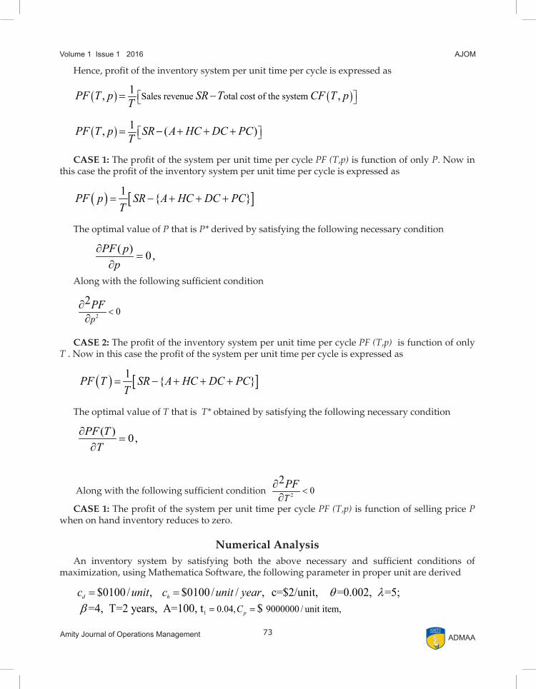
Hence, profit of the inventory system per unit time per cycle is expressed as
( ) ( )Sales revenue otal cost of the system 1, ,PF T p SR T CF T pT = −
( ) 1, ( )PF T p SR A HC DC PCT = − + + +
CASE 1: The profit of the system per unit time per cycle PF (T,p) is function of only P. Now in this case the profit of the inventory system per unit time per cycle is expressed as
( ) [ ]1 { }PF p SR A HC DC PCT
= − + + +
The optimal value of P that is P* derived by satisfying the following necessary condition
( ) 0,PF pp
∂=
∂Along with the following sufficient condition
2 0
2pPF
<∂
∂
CASE 2: The profit of the inventory system per unit time per cycle PF (T,p) is function of only T . Now in this case the profit of the system per unit time per cycle is expressed as
( ) [ ]1 { }PF T SR A HC DC PC
T= − + + +
The optimal value of T that is T* obtained by satisfying the following necessary condition
( ) 0,PF T
T∂
=∂
Along with the following sufficient condition 2 02
TPF
<∂∂
CASE 1: The profit of the system per unit time per cycle PF (T,p) is function of selling price P when on hand inventory reduces to zero.
Numerical AnalysisAn inventory system by satisfying both the above necessary and sufficient conditions of
maximization, using Mathematica Software, the following parameter in proper unit are derived
1 0.04, 9000000 / unit item,
$0100/ , $0100/ / , c=$2/unit, =0.002, =5; =4, T=2 years, A=100, t $
d h
pCc unit c unit year q lb = =
= =
74 Amity Journal of Operations ManagementADMAA
Volume 1 Issue 1 2016AJOM
Using the above parameter the optimal selling price P* and the optimal profit of the system PF per cycle respectively is calculated as
The optimal selling price 7* $ 1.10573 10 ,p = ×
Optimal profit of the system per cycle * 11$ 2.16312 10 ,PF = ×
CASE 2: The profit of the system per unit time per cycle PF (T,p) is function of time T per cycle only when on hand inventory reduces to zero.
Numerical AnalysisAn inventory system by satisfying both the above necessary and sufficient conditions of
maximization, using Mathematica Software, the following parameter in proper unit are derived
1unit item 0.08, / unit item,
$01/ , $01/ / , =0.002, =2; =2, p=$30/ , A=100, t $ 20
d h
pCc unit c unit year q lb = =
= =
Using the above parameter the optimal time T* per cycle and the optimal profit of the system PF per cycle respectively is calculated as
The optimal time per cycle * 0.8967 ,T year=
Optimal profit of the system per cycle * $ 4670.88,PF =
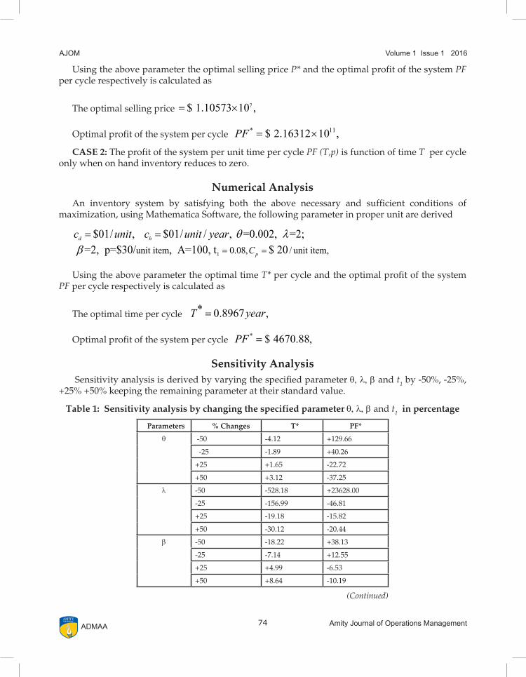
Sensitivity Analysis Sensitivity analysis is derived by varying the specified parameter q, l, b and t1 by -50%, -25%,
+25% +50% keeping the remaining parameter at their standard value.
Table 1: Sensitivity analysis by changing the specified parameter q, l, b and t1 in percentage
Parameters % Changes T* PF*
q -50 -4.12 +129.66
-25 -1.89 +40.26
+25 +1.65 -22.72
+50 +3.12 -37.25
l -50 -528.18 +23628.00
-25 -156.99 -46.81
+25 -19.18 -15.82
+50 -30.12 -20.44
b -50 -18.22 +38.13
-25 -7.14 +12.55
+25 +4.99 -6.53
+50 +8.64 -10.19
(Continued)
75Amity Journal of Operations Management
Volume 1 Issue 1 2016 AJOM
ADMAA
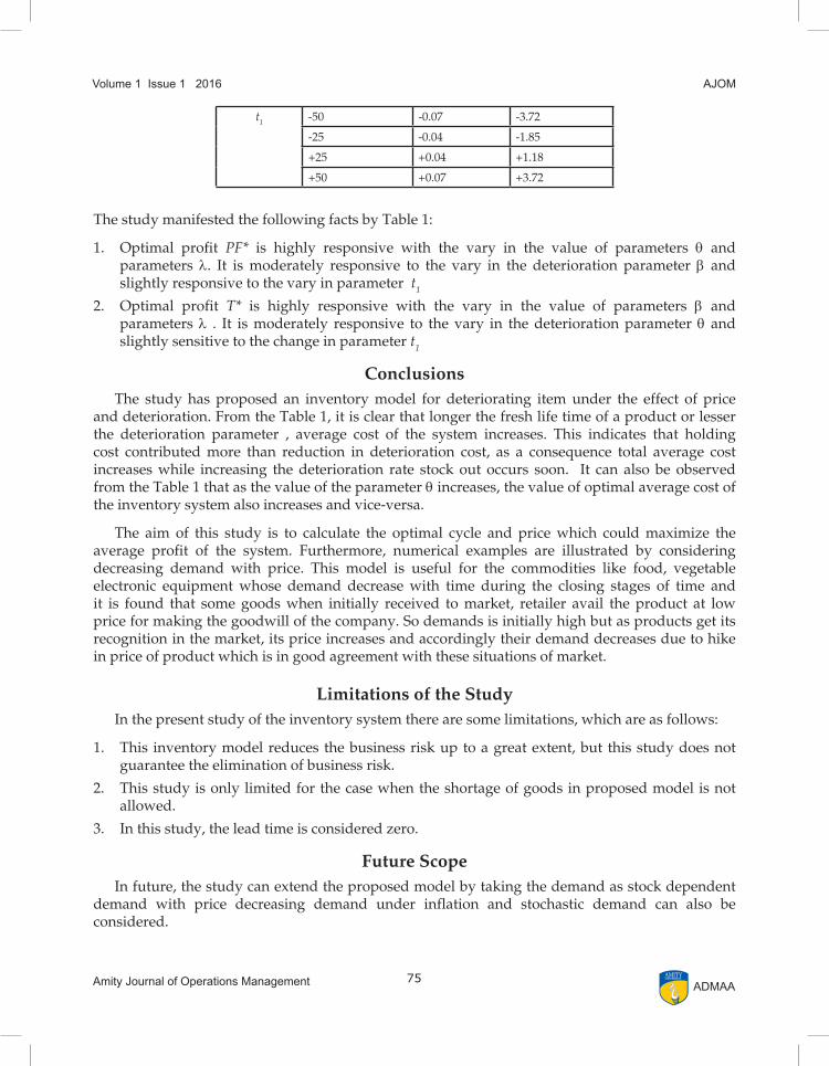
t1 -50 -0.07 -3.72
-25 -0.04 -1.85
+25 +0.04 +1.18
+50 +0.07 +3.72
The study manifested the following facts by Table 1:
1. Optimal profit PF* is highly responsive with the vary in the value of parameters q and parameters l. It is moderately responsive to the vary in the deterioration parameter b and slightly responsive to the vary in parameter t1
2. Optimal profit T* is highly responsive with the vary in the value of parameters b and parameters l . It is moderately responsive to the vary in the deterioration parameter q and slightly sensitive to the change in parameter t1
ConclusionsThe study has proposed an inventory model for deteriorating item under the effect of price
and deterioration. From the Table 1, it is clear that longer the fresh life time of a product or lesser the deterioration parameter , average cost of the system increases. This indicates that holding cost contributed more than reduction in deterioration cost, as a consequence total average cost increases while increasing the deterioration rate stock out occurs soon. It can also be observed from the Table 1 that as the value of the parameter q increases, the value of optimal average cost of the inventory system also increases and vice-versa.
The aim of this study is to calculate the optimal cycle and price which could maximize the average profit of the system. Furthermore, numerical examples are illustrated by considering decreasing demand with price. This model is useful for the commodities like food, vegetable electronic equipment whose demand decrease with time during the closing stages of time and it is found that some goods when initially received to market, retailer avail the product at low price for making the goodwill of the company. So demands is initially high but as products get its recognition in the market, its price increases and accordingly their demand decreases due to hike in price of product which is in good agreement with these situations of market.
Limitations of the StudyIn the present study of the inventory system there are some limitations, which are as follows:
1. This inventory model reduces the business risk up to a great extent, but this study does not guarantee the elimination of business risk.
2. This study is only limited for the case when the shortage of goods in proposed model is not allowed.
3. In this study, the lead time is considered zero.
Future ScopeIn future, the study can extend the proposed model by taking the demand as stock dependent
demand with price decreasing demand under inflation and stochastic demand can also be considered.
76 Amity Journal of Operations ManagementADMAA
Volume 1 Issue 1 2016AJOM
ReferencesDeb, M., & Chaudhuri, K. S. (1986). An EOQ model for items with finite rate of production and variable rate
of deterioration. Opsearch, 23(1), 175-181.
Ghare, P. M., & Schrader, G. F. (1963). A model for exponentially decaying inventory. Journal of Industrial Engineering, 14(5), 238-243.
Kaur, J., & Sharma, R. (2012). Inventory model: Deteriorating items with price and time dependent demand rate. International Journal of Modern Engineering Research, 2(5), 3650-3652.
Kumar, S., & Singh, A, K. (2015). An optimal replenishment policy for non instantaneous deteriorating items with stock dependent, price decreasing demand and partial backlogging. Indian Journal of Science and Technology, 8(35), 1-11.
Min, J., Zhou, Y. W., & Zhao, J. (2010). An inventory model for deteriorating items under stock-dependent demand and two-level trade credit. Applied Mathematical Modelling, 34(11), 3273-3285.
Mondal., S. K., Dey, J. K., & Maiti, M. (2007). A single period inventory model of a deteriorating item sold from two shops with shortage via genetic algorithm. Yugoslav Journal of Operations Research, 17(1), 75-94.
Author’s Profile
Shiv Kumar is currently pursuing his research in Operations Research from Indian School of Mines Dhanbad, Jharkhand, India. His major research interests include inventory models, optimization techniques. He has published 4 papers in international journals and presented 4 papers are in various conferences.


![Deteriorating Items Inventory Model with Different ... · inventory model with constant rate of deterioration. Covert and Philip [3] extended the model by considering variable rate](https://img.pdfslide.us/doc/110x75/5ea274f61d5524034c7359ff/deteriorating-items-inventory-model-with-different-inventory-model-with-constant.jpg)