Optimization of data flow execution in a parallel environment

Distributed and Parallel Databases (2019) 37:385–410https://doi.org/10.1007/s10619-018-7243-3

Optimization of data flow execution in a parallelenvironment

Georgia Kougka1 · Anastasios Gounaris1

Published online: 22 August 2018© Springer Science+Business Media, LLC, part of Springer Nature 2018

AbstractAlthough the modern data flows are executed in parallel and distributed environments,e.g. on a multi-core machine or on the cloud, current cost models, e.g., those consid-ered by state-of-the-art data flow optimization techniques, do not accurately reflectthe response time of real data flow execution in these execution environments. Thisis mainly due to the fact that the impact of parallelism, and more specifically, theimpact of concurrent task execution on the running time is not adequately modeled incurrent cost models. The contribution of this work is twofold. Firstly, we propose anadvanced costmodel that aims to reflect the response time of a data flow that is executedin parallel more accurately. Secondly, we show that existing optimization solutionsare inadequate and develop new optimization techniques targeting the proposed costmodel. We focus on the single multi-core machine environment provided by modernbusiness intelligence tools, such as Pentaho Kettle, but our approach can be extendedto massively parallel and distributed settings. The distinctive features of our proposalis that we model both time overlaps and the impact of concurrency on task runningtimes in a combined manner; the latter is appropriately quantified and its significanceis exemplified. Furthermore, we propose extensions to current optimizers that decideon the exact ordering of flow tasks taking into account the new optimization metric.Finally, we evaluate the new optimization algorithms and show up to 59% responsetime improvement over state-of-the-art task ordering techniques.

Keywords Data flow optimization · Cost modeling · Task ordering

B Anastasios [email protected]

Georgia [email protected]

1 Department of Informatics, Aristotle University of Thessaloniki, Thessaloníki, Greece

123

http://crossmark.crossref.org/dialog/?doi=10.1007/s10619-018-7243-3&domain=pdf

386 Distributed and Parallel Databases (2019) 37:385–410

1 Introduction

Nowadays, data flows constitute an integral part of data analysis. The modern dataflows are complex and executed in parallel systems, such as multi-core machines orclusters employing a wide range of diverse platforms like Pentaho Kettle,1 Spark2 andFlink3 to name a few. These platforms operate in a manner that involves significanttime overlapping and interplay between the constituent tasks in a flow. However, thereare no cost models that provide analytic formulas for estimating the response time(wall-clock time) of a flow in such platforms. Cost models, apart from being usefulin their own right, are encapsulated in cost-based optimizers; currently, for example,cost-based optimization solutions for task ordering in data flows employ simple costmodels that may not capture the flow execution running time accurately, as shown inthis work. For example, the sum cost metric, which is employed by many state-of-the-art task ordering techniques [17,20,30], merely sums the cost of individual tasks.This results in an execution cost computation that may deviate from the real executiontime, and the corresponding optimizations may not be reflected on response time.Consequently, there is a need for employing new data flow optimization solutions thattake into consideration a cost model during the optimization decision phase that istailored to response time minimization.

Typically, cost models rely on the existence of appropriate metadata regarding eachtask, which are combined using simple algebraic formulas with the sum and maxoperations. Most often, task metadata consider the cost of each task, which is com-mensurate with the task running time if executed in a stand-alone manner. The mainchallenges in devising a cost model for running time that is appropriate for moderndata flow execution stem from the following factors: (i) many tasks are executed in par-allel employing all three main forms of parallelism, namely, partitioned, pipelined andindependent, and the resulting time overlaps, which entail that certain task executionsdo not contribute to the overall running time, need to be reflected in the cost model;and (ii) computation resources are shared among multiple tasks, and the concurrentexecution of tasks using the same resource pool impacts on their execution costs.

In this work, we initially focus on a single multi-core machine environment, suchas Pentaho Data Integration (PDI, aka Kettle). First, we devise a cost model that canbe used to estimate the response time, when the data flows are executed in paralleland distributed execution environments. Then, we show the inadequacy of the exist-ing task ordering optimization algorithms and propose a new optimization algorithmthat decides the best order of executing the tasks of a flow employing the proposedcost model. Regarding the proposed model, we build upon existing cost modelingtechniques that tend to consider time overlapping (e.g., [1,2,6,23,31,33]), but not theinterplay between task costs. In order to achieve this, we propose a solution in whichthe cost of each task is weighted according to the number of concurrent tasks takinginto account constraints of execution machines, such as capacity in terms of numberof cores. Then, we show cases, in which the existing optimization solutions fail to

1 http://community.pentaho.com/projects/data-integration.2 http://spark.apache.org/.3 http://flink.apache/.

123

http://community.pentaho.com/projects/data-integration.

http://spark.apache.org/.

http://flink.apache/.

Distributed and Parallel Databases (2019) 37:385–410 387

improve the response time of a flow execution and, to ameliorate this, we introducenew optimization techniques that utilize the more advanced cost model and build uponthe effective combination of optimization techniques in [20,33]. The results of the opti-mization improvements are thoroughly validated. More specifically, the contributionis as follows:4

1. We explain and provide experimental evidence on why the existing cost modelsprovide estimates that may widely deviate from the real execution time of modernworkflows.

2. We propose a model that not only considers overlapping task executions but alsoquantifies the correlation between task costs due to concurrent allocation to thesame processing unit. The model is execution engine software- and data flowtype-independent.

3. We show how our model applies to example flows in PDI, where inaccuracies ofup to 50% are observed if the impact of concurrency is not considered.

4. We explain why the state-of-the-art optimization algorithms may fail to optimizethe response time of a data flow execution.

5. We propose new task ordering optimization techniques that leverage the costmodelto decrease running time.

6. We conduct a thorough evaluation of the new optimization techniques and theresults show that improvements can reach 59% over state-of-the art techniquesthat aim at minimizing response time indirectly, through minimizing resourceconsumption (sumcostmetric). The average improvements over a group of randominitial valid flows can be up to 4.87 times for flows with 24 tasks.

In the remainder of this section we provide background on flow parallelization, theassumptions regarding the execution environment that we consider and a discussionabout the inadequacy of cost models employed in data flow optimization. We continuethe discussion of related work in Sect. 2. In Sect. 3 we introduce the notation. Ourmodeling proposal is presented in detail in Sect. 4, while the in Sect. 5, we introduce thenew task ordering optimization solutions. In Sect. 6, we show experimental evaluationfindings based on extensive simulation. We discuss the barriers and challenges ofapplying and incorporating the proposed optimization techniques in tools such as PDIin Sect. 7. We summarize the conclusions in Sect. 8.

1.1 Parallelizing data flows

The parallel execution of a data flow exploits three types of parallelism, namely inter-operator (pipelined), intra-operator (partitioned) and independent parallelism. Here,we use the terms task and operator interchangeably. These types of parallelizationare well-known in query optimization [9], and used to decrease the response time ofa data flow execution.

The intra-operation parallelism considers the parallelization of a single task of adata flow. This type of parallelization is defined by the instantiation of a logical task as

4 An early version of this work containing themodelingmaterial but no optimization solutions has appearedin [19]. The novel material in this work compared to the preliminary version is in Sects. 5, 6 and 7, whileSect. 2 has been also extended accordingly.

123


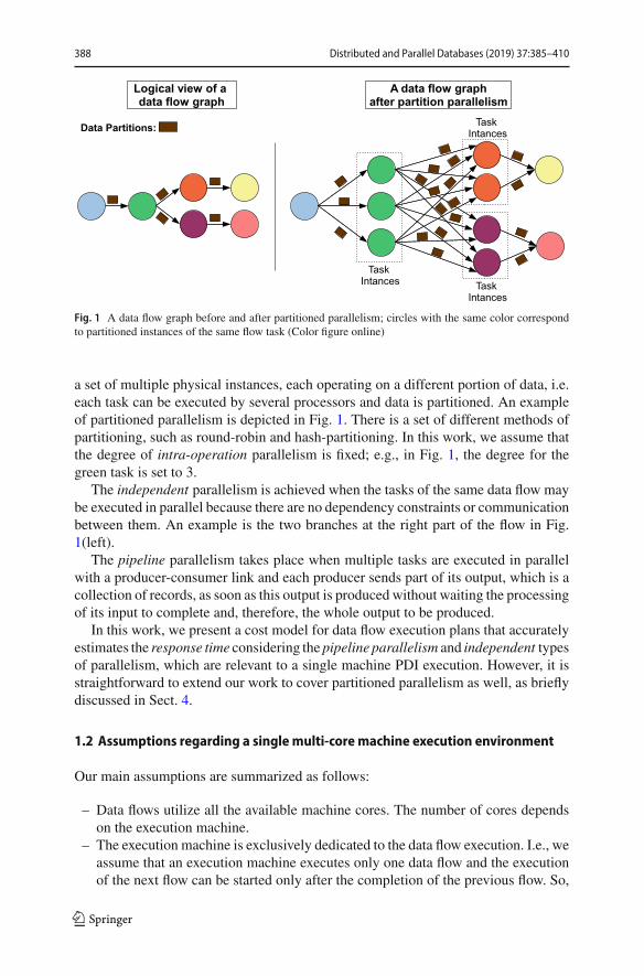
Fig. 1 A data flow graph before and after partitioned parallelism; circles with the same color correspondto partitioned instances of the same flow task (Color figure online)

a set of multiple physical instances, each operating on a different portion of data, i.e.each task can be executed by several processors and data is partitioned. An exampleof partitioned parallelism is depicted in Fig. 1. There is a set of different methods ofpartitioning, such as round-robin and hash-partitioning. In this work, we assume thatthe degree of intra-operation parallelism is fixed; e.g., in Fig. 1, the degree for thegreen task is set to 3.

The independent parallelism is achieved when the tasks of the same data flow maybe executed in parallel because there are no dependency constraints or communicationbetween them. An example is the two branches at the right part of the flow in Fig.1(left).

The pipeline parallelism takes place when multiple tasks are executed in parallelwith a producer-consumer link and each producer sends part of its output, which is acollection of records, as soon as this output is produced without waiting the processingof its input to complete and, therefore, the whole output to be produced.

In this work, we present a cost model for data flow execution plans that accuratelyestimates the response time considering the pipeline parallelism and independent typesof parallelism, which are relevant to a single machine PDI execution. However, it isstraightforward to extend our work to cover partitioned parallelism as well, as brieflydiscussed in Sect. 4.

1.2 Assumptions regarding a single multi-core machine execution environment

Our main assumptions are summarized as follows:

– Data flows utilize all the available machine cores. The number of cores dependson the execution machine.

– The execution machine is exclusively dedicated to the data flow execution. I.e., weassume that an execution machine executes only one data flow and the executionof the next flow can be started only after the completion of the previous flow. So,

123


the available machine executes tasks and stores data for a single data flow at atime.

– Multiple tasks of a data flow are executed simultaneously through multi-threadingthat allows multiple threads to be employed during flow processing. More specif-ically, we assume a form of multi-threaded execution, in which each task spawnsa separate thread, running on a core decided by the underlying operating systemscheduler. Obviously, if two task threads share the same core, they are executedconcurrently but not simultaneously.

– The execution engine exploits pipeline and independent parallelism to the largestpossible extent; i.e., the default engine configuration regarding task executionoperates in a mode, according to which flow tasks are aggressively scheduled assoon as their input data is available.

The assumptions above hold also for massive parallel settings. The main differenceis that, in massive parallelism settings, partitioned parallelism typically applies.

1.3 Motivation for devising a new cost model for task ordering optimization

Amain application of cost models is in cost-based optimization. One of forms of dataflow optimization that has been largely explored in the data management literature istask re-ordering. Taking this type of optimization as our case study, we can observefrom the survey in [20] that the corresponding techniques target one of the followingoptimization objectives:

1. Sum Cost Metric of the Full plan (SCM-F): minimize the sum of the task andcommunication costs of a data flow [13,16,17,22,28,30,31,36].

2. Sum Cost Metric of the Critical Path (SCM-CP): minimize the sum of the task andcommunication costs along the flow’s critical path [1,2].

3. Bottleneck: minimize the highest task cost [1,2,31,33].4. Throughput: maximize the throughput (number of records processed per time unit)

[8].

The first three metrics and the associated cost models can capture the response timeunder specific assumptions only. The response time represents the wall-clock timefrom the beginning until the end of the flow execution. SCM-F defines the responsetimewhen the tasks of a data flow are executed sequentially; for examplewhen all tasksare blocking. Another case is when tasks are pipelined but are executed on the sameCPU core (processor). In that case, the SCM-F may serve as a good approximation ofthe response time. SCM-CP reflects the response timewhen the data flow branches areexecuted independently and the tasks of each branch are executed sequentially. Finally,bottleneck represents the response timewhen all the tasks of the flow are executed in apipelined manner and each task is executed on a different processor assuming enoughcores are available.

So,whydoweneed another costmodel? PDI, Flink, Spark and similar environmentsaggressively employ pipeline parallelism potentially on multiple processors. Conse-quently, the SCM-F and SCM-CP cost metrics do not correspond to the responsetime of the flow execution. In general, SCM-F indirectly aims to capture resource

123


consumption; since the modern execution engines are advanced enough to performsophisticated resource usage and avoid resource under-utilization, minimizing theresource consumption may be correlated to minimizing the response time in somecases on a single multi-core machine, but as shown later, this does not always holdand moreover, it is rare in a setting employing multiple machines. The bottleneckcost metric is not appropriate either. This is because there are pipelined tasks that areexecuted on the same processor, but also there are tasks that are blocking, e.g., sort.So, for estimating response time, we need to employ a new cost metric that explicitlyconsiders parallelism and the corresponding overlaps in task execution.

Furthermore, a more accurate cost model for describing the response time is signif-icant in its own right even when not used to drive optimizations. It allows us to betterunderstand the flow execution and provides better insights into the details involved.Moreover, as will be shown in the subsequent section, merely considering time over-laps does not suffice, because the task costs are correlated during concurrent taskexecution.

2 Related work

We split the related work into two parts to discuss cost models and task re-ordering,respectively.

Cost modeling. The main limitation of existing cost models is that, even if theyconsider overlapped execution, they assume that the cost of each task remains fixedindependently ofwhether other tasks are executing concurrently sharingCPU,memoryand other resources. Examples that fall in this category are the work in [23], whichtargets a cloud environment for scientific workflow execution, and in [6]. The costmodel in the latter considers that the flow is represented by a graph with multiplebranches (or paths), where the tasks in each path are executed sequentially andmultiplebranches are executed in parallel. In contrast, we cover more generic cases.

Additionally, several proposals based on the traditional cost models have beenpresented in order to capture the execution of MapReduce jobs. For example, a perfor-mancemodel that estimates the job completion time is presented for ARIAFrameworkin [35]; this solution accounts for the fact that the map and reduce phases are executedsequentially employing partitioned parallelism but do not take into account the effectof allocation of multiple map/reduce tasks on the same core. The same rationale is alsoadapted by cost models introduced in proposals, such as [37] and [32]. Nevertheless,an interesting feature of these models is that theymodel the real-world phenomenon ofimbalanced task partition running times. In theMapReduce setting, the authors in [29]propose the Produce-Transporter-Consumer model to define the parallel execution ofMapReduce tasks. The key idea is to provide a cost model that describes the tradeoffsof four factors (namely, map and reduce waves, output compression of map tasks andcopy speed during data shuffling) considering any overlaps. As previously, the impactof concurrency is neglected. Other works for MapReduce, such as [3], suffer from thesame limitations.

Task ordering. Data flow optimization is a multi-dimensional area; broadly, opti-mizations are divided into two main categories, those referring to the logical (or

123


conceptual) level and those referring to the low-level physical execution layer [20].In the first category, the corresponding techniques employ task ordering, introduc-tion, removal, merge and decomposition. In the latter, they focus on choosing the taskimplementation, execution engine and its configuration among several alternatives.In this work, we focus on task ordering, which refers to the logical level of the flowdescription but requires an underlying cost model that considers the low-level physicalexecution details.

A significant number of techniques that optimize the flow execution plan throughchanges in the structure of the flow graph including task ordering mechanism havebeen presented in the literature. The key characteristic of these proposals is that theyconsider other cost models than response time during optimization decisions, such asbottleneck and sum cost metric. For example, there are flow optimization solutionsthat are inspired by query processing techniques. In [10], an optimization algorithm forquery planswith dependency constraints between algebraic operators is presented. Thetechniques in [17] build on top of [14,21], and are shown to be superior to approaches,such as [5,12,15,22,26,30,36] when SCM-F is targeted. In [18], an exhaustive opti-mization proposal for data flows is presented that aims to produce all the topologicalsortings of the tasks in a way that each sorting is produced from the previous one withthe minimal amount of changes. This technique can be adapted for minimizing theresponse time, but is not scalable for data flows with high number of tasks and espe-cially, for flows that preserve only a few dependency constraints between tasks. Anearly idea of metric combination was presented in [31], where the pipelining segmentsare grouped and for these sub-flows, the response time equals to the bottleneck met-ric. Then SCM-F is minimized for these segments of pipelining tasks. However, thepipelined segments are not optimized and independent parallelism is not considered.

Another interesting approach to flow optimization is presented in [13], where theoptimizations are based on the analysis of the properties of user-defined functions thatimplement the data processing logic. This work focuses mostly on techniques thatinfer the dependency constraints between tasks through examination of their internalsemantics rather than on task re-ordering algorithms per se. In general, automatedextraction of statistical and semantic task metadata is of key significance in order taskre-ordering techniques to find their way into business data flow execution platforms.

3 Preliminaries

A data flow is represented as a Directed Acyclic Graph (DAG), where each vertexcorresponds to a task of the flow and the edges between vertices represent the com-munication among tasks (intermediate data shipping among tasks). In data flows, theexchange of data between tasks is explicitly represented through edges. We assumethat the data flows can have multiple sources and multiple sinks. A source of a dataflow corresponds to a task with no incoming edges, while a sink corresponds to a taskwith no outgoing edges. The main notation and assumptions are as follows:

Let G = (V , E) be a Directed Acyclic Graph (DAG), where V = t1, t2, . . . , tndenotes the vertices of the graph (data flow tasks) and E represents the edges (flowof data among the tasks); n is the total number of vertices. Each vertex corresponds

123


to a data flow task and is responsible for one or both of the following: (i) reading orstoring data, and (ii) manipulating data. The tasks of a data flow may be complex dataanalysis tasks, but may also execute traditional relational operations, such as unionand join. Each edge equals to an ordered pair (v j , vk), which means that task t j sendsdata to task tk .

Each data flow is characterized by the following metadata:

– Cost (ci ), which applies to each task. The ci corresponds to the cost for processingall the input records that the ti task receives taking into consideration the requiredCPU cycles and disk I/Os. In distributed systems, the cost of network traffic needsto be considered as well, and may be the most important factor. An essentiallysimilar consideration is ci to denote the cost per single input record. In the lattercase, the selectivity (sel) information of all tasks is needed in order to derive thesize of the task input and then, the task cost for its entire input; the selectivitydenotes the average number of returned data items per source tuple.

– CommunicationCost (cci→ j ), whichmay apply to edges. The communication costof data shipping between the ti and t j depends on either the forward local pipelineddata transfer between tasks or the data shuffling between parallel instances of thesame data flow. It does not include any communication-related cost included in ci ;it includes only the cost that is dependent on both ti and t j rather than only on ti .

– Parallelism Type of Task (pti ), which describes the type of parallelism of a task i ,when the task is executed. More specifically, the parallelism type characterizes ifa data flow task is executed in a pipelined, denoted as p or no pipelined manner(blocking task), denoted as np. A blocking task requires all the tuples of the inputdata in order to start producing results; i.e., the parallelism type of a task reflectsthe way a task process the input data and produces its output.

Note that the modeling of the flow as described above is independent of the inputdata types, which can be relational records, semi-structured documents or plain textitems.

4 A cost model for data flow response time

First, we describe a model for a single-machine setting and finally, we generalize todistributed settings.

4.1 Models for a single multi-core machine

We start by examining simple flows andwe gradually extend our observations to largerand more complicated ones.

4.1.1 A linear flowwith a single pipelined segment of n tasks

A pipeline segment is defined by a sequence of n tasks in a chain, where the firsttask is either a source or a child of a blocking task. The last task is either a sink or a

123


blocking task; both types of tasks do not allow flow of output records in a pipelinedmanner downstream.Additionally, the tasks in between are all of p type. Also, pipelinesegments do not overlap with regards to the vertices they cover. Such segments benefitfrom inter-operator parallelism. The key point of our approach is to account for the factthat there is non-negligible interference between tasks. This interference is capturedby the variable α. Let us suppose that our machine has m cores. In the case wheren ≤ m, each task thread can execute on a separate core exclusively. The cost modelthat estimates the response time (RT) of a data flow execution is defined as follows,which aims to capture the fact that the running times of tasks overlap.

Response T ime (RT ) = αmax{c1, . . . , cn} (1)

In general, the parameter α is a weight that aims to abstract the impact of multi-threading in a single metric. Multi-threading may lead to performance overhead dueto several factors, such as the context switching between threads, as the flow tasks areexecuted concurrently and need to switch from one thread to another multiple times.An additional factor for response time increase is due to the locks that temporarilyrestrict tasks sharing memory to write to the same memory location. Finally, themost significant factor in the terms of affecting the response time is the contentionthat captures the interference of the multiple interactions of each data flow task withmemory and disk. Specifically, when there are multiple requests to memory, this mayresult in exceeding memory bandwidth and consequently, to RT increase. Finally,allocating and scheduling threads incurs some overhead, which, however, is negligiblein most cases. Instead of devising complex cost models for all the above factors, inthis work, we have decided to cover all of them by using a single parameter, whichcan be computed empirically through experiments.

Nevertheless, multi-threading execution leads to execution cost improvementbecause of the parallel task execution. So, we may observe RT minimization, whenall or more of the available cores are exploited by the data flow tasks and one copyof data is used by multiple threads at the same time. Also, the delays occurred bytransferring data from memory and disk are overlapped by the task execution, whenthe number of tasks is higher than the available execution units. In general, cache-levelconfiguration may heavily impact on RT . As previously, all these factors are reflectedon the α parameter.

Let us consider now the case where n > m and the task threads need to share theavailable cores in order to be executed. In this case, each core may execute more thanone task and the RT is determined by all the flow tasks. An exception is when thereis a single task with cost higher than the sum of all the other costs (similarly to themodeling in [35]):

Response T ime (RT ) = αmax{max{c1, .., cn},∑{c1, . . . , cn}

m} (2)

4.1.2 Experiments in PDI

In the following, we present a set of experiments that we conducted in order to under-stand the role of α in RT estimation according to Eqs. (1) and (2). We consider

123


synthetic flows in PDI with n = 1, . . . , 26 tasks and an additional source task. Theinput ranges from 2.4M to 21.8M records. Two machines are used, with (i) a 4-core/4-thread i5 processor; and (ii) a 4-core/8-thread i7 processor, respectively. Finally, thetask types are two, either homogenous or heterogeneous. In the former case, all taskshave the same cost (denoted as equal). In the latter case (denoted as mixed), half ofthe tasks have the same cost as in the equal case, and the other tasks have anothercost, which is lower by an order of magnitude. All the tasks apply filters to the inputdata, but these filters are not selective in the sense that they produce the same data thatthey receive; they just incur processing cost. The data input is according to the TPC-DI Benchmark[25] and we consider records taken from the implementation in http://www.essi.upc.edu/dtim/blog/post/tpc-di-etls-using-pdi-aka-kettle. Each experimentrun was repeated 5 times and the median times are reported; in all experiments thestandard deviation was negligible.

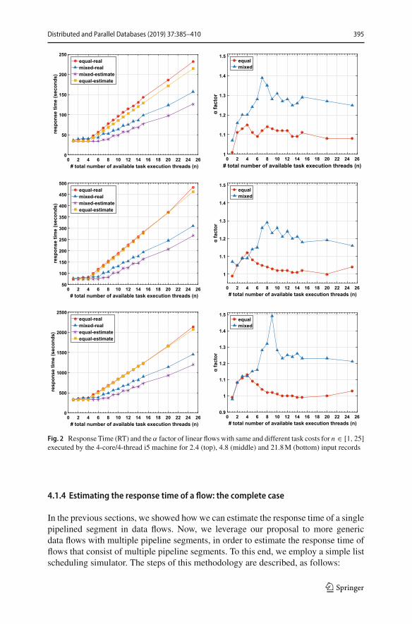
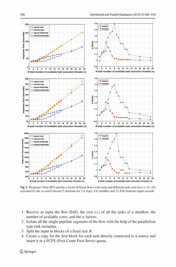
The left column of Figs. 2 and 3 shows how the response time of the two differenttypes of data flows evolves as the number of tasks, and consequently the number ofexecution threads, increases. It also shows what the cost model estimates would be ifno weights were considered. Themain observation is twofold. First, the response time,as expected from Eqs. (1) and (2), stays approximately stable when n ≤ m, and then,grows linearly when n > m. This behavior does not change with the increase in thedata size. Second, estimates with no weights can underestimate the running time byup to 50%, whereas there are also cases when they overestimate the running times bya smaller factor (approx. 5%). More importantly, the main inaccuracies are observedin the mixed-cost case, which is more common in practice.

The α factor is shown in the right column of Figs. 2 and 3. Values both lower andhigher than 1 are observed. Although α captures the combination of overhead andimprovement causes described in the previous section, the importance of each causevaries. In values greater than 1, resource contention is dominating; whereas, in valueslower than 1, the fact that waits for resources are hidden outweighs any overheads.The main observations are as follows: (i) the α factor varies significantly for the samedataset when the number of tasks is modified; (ii) α can be of significant magnitudecorresponding to more than 50% increase in the task costs; (iii) for flows that consistof up to 4 tasks with equal cost, the α factor continuously grows (i.e., contention isdominating) and then, when the number of tasks further increases, the behavior differsbetween cases; and (iv) for data flows with different task costs and n > m, the α factorincreases sharply for flows with up to 7-9 tasks depending on the input data size.

4.1.3 A linear flowwith multiple independent pipelined segments

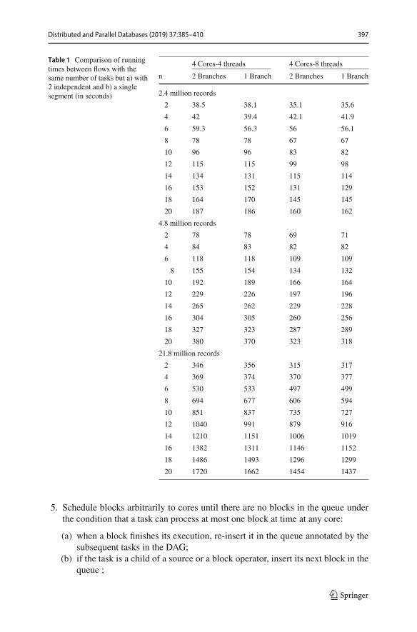
In Table 1, we show the running times of flows with the same number of tasks when alltasks belong to a single pipelined segment and when there are two segments belongingto two different branches originating from the same source, according to the fork tem-plate in [34]. We can observe that the running times are similar. From this observation,we can draw the conclusion that the magnitude of the weights (i.e., the wc and thecorresponding α factors) depend on the number of concurrent tasks and need not besegment-specific; that is, it is safely to assume that all concurrent tasks share the samefactors.

123

http://www.essi.upc.edu/dtim/blog/post/tpc-di-etls-using-pdi-aka-kettle

http://www.essi.upc.edu/dtim/blog/post/tpc-di-etls-using-pdi-aka-kettle


0 2 4 6 8 10 12 14 16 18 20 22 24 26# total number of available task execution threads (n)

0

50

100

150

200

250re

spon

se ti

me

(sec

onds

)equal-realmixed-realmixed-estimateequal-estimate


1

1.1

1.2

1.3

1.4

1.5equalmixed


50

100

150

200

250

300

350

400

450

500

resp

onse

tim

e (s

econ

ds)

equal-realmixed-realmixed-estimateequal-estimate


1

1.1

1.2

1.3

1.4

1.5equalmixed


0

500

1000

1500

2000

2500

resp

onse

tim

e (s

econ

ds)

equal-realmixed-realequal-estimateequal-estimate


0.9

1

1.1

1.2

1.3

1.4

1.5equalmixed

Fig. 2 Response Time (RT) and the α factor of linear flowswith same and different task costs for n ∈ [1, 25]executed by the 4-core/4-thread i5 machine for 2.4 (top), 4.8 (middle) and 21.8M (bottom) input records

4.1.4 Estimating the response time of a flow: the complete case

In the previous sections, we showed howwe can estimate the response time of a singlepipelined segment in data flows. Now, we leverage our proposal to more genericdata flows with multiple pipeline segments, in order to estimate the response time offlows that consist of multiple pipeline segments. To this end, we employ a simple listscheduling simulator. The steps of this methodology are described, as follows:

123



0

50

100

150

200

250re

spon

se ti

me

(sec

onds

)equal-realmixed-realequal-estimatemixed-estimate


0.9

1

1.1

1.2

1.3

1.4

1.5

1.6equalmixed


50

100

150

200

250

300

350

400

450

resp

onse

tim

e (s

econ

ds)

equal-realmixed-realequal-estimatemixed-estimate


0.9

1

1.1

1.2

1.3

1.4

1.5

1.6equalmixed


200

400

600

800

1000

1200

1400

1600

1800

2000

resp

onse

tim

e (s

econ

ds)

equal-realmixed-realequal-estimatemixed-estimate


0.9

1

1.1

1.2

1.3

1.4

1.5

1.6equalmixed

Fig. 3 Response Time (RT) and the α factor of linear flowswith same and different task costs for n ∈ [1, 25]executed by the 4-core/8-thread i7 machine for 2.4 (top), 4.8 (middle) and 21.8M (bottom) input records

1. Receive as input the flow DAG, the cost (ci ) of all the tasks of a dataflow, thenumber of available cores, and the α factors.

2. Isolate all the single-pipeline segments of the flow with the help of the parallelismtype task metadata.

3. Split the input in blocks of a fixed size B.4. Create a copy for the first block for each task directly connected to a source and

insert it in a FCFS (First Come First Serve) queue.

123


Table 1 Comparison of runningtimes between flows with thesame number of tasks but a) with2 independent and b) a singlesegment (in seconds)

4 Cores-4 threads 4 Cores-8 threads

n 2 Branches 1 Branch 2 Branches 1 Branch

2.4 million records

2 38.5 38.1 35.1 35.6

4 42 39.4 42.1 41.9

6 59.3 56.3 56 56.1

8 78 78 67 67

10 96 96 83 82

12 115 115 99 98

14 134 131 115 114

16 153 152 131 129

18 164 170 145 145

20 187 186 160 162

4.8 million records

2 78 78 69 71

4 84 83 82 82

6 118 118 109 109

8 155 154 134 132

10 192 189 166 164

12 229 226 197 196

14 265 262 229 228

16 304 305 260 256

18 327 323 287 289

20 380 370 323 318

21.8 million records

2 346 356 315 317

4 369 374 370 377

6 530 533 497 499

8 694 677 606 594

10 851 837 735 727

12 1040 991 879 916

14 1210 1151 1006 1019

16 1382 1311 1146 1152

18 1486 1493 1296 1299

20 1720 1662 1454 1437

5. Schedule blocks arbitrarily to cores until there are no blocks in the queue underthe condition that a task can process at most one block at time at any core:

(a) when a block finishes its execution, re-insert it in the queue annotated by thesubsequent tasks in the DAG;

(b) if the task is a child of a source or a block operator, insert its next block in thequeue ;

123


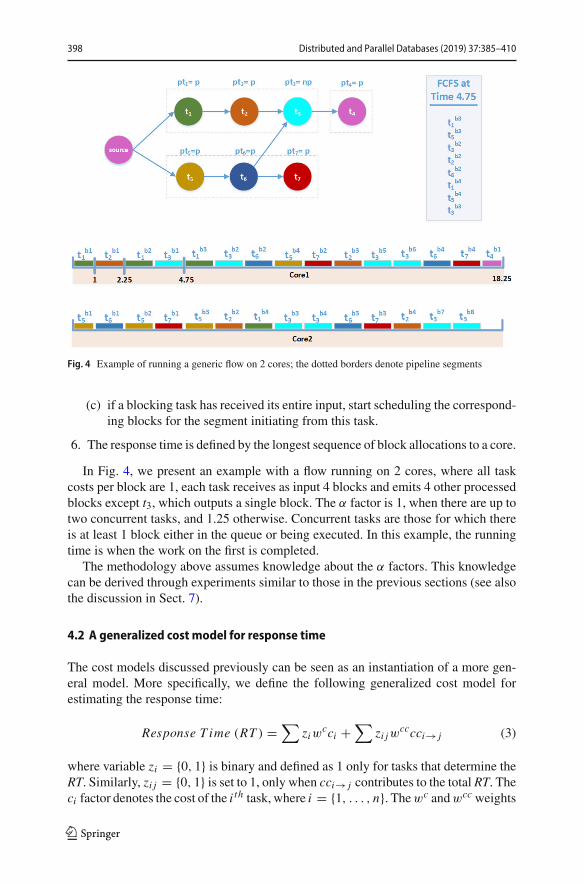
Fig. 4 Example of running a generic flow on 2 cores; the dotted borders denote pipeline segments

(c) if a blocking task has received its entire input, start scheduling the correspond-ing blocks for the segment initiating from this task.

6. The response time is defined by the longest sequence of block allocations to a core.

In Fig. 4, we present an example with a flow running on 2 cores, where all taskcosts per block are 1, each task receives as input 4 blocks and emits 4 other processedblocks except t3, which outputs a single block. The α factor is 1, when there are up totwo concurrent tasks, and 1.25 otherwise. Concurrent tasks are those for which thereis at least 1 block either in the queue or being executed. In this example, the runningtime is when the work on the first is completed.

The methodology above assumes knowledge about the α factors. This knowledgecan be derived through experiments similar to those in the previous sections (see alsothe discussion in Sect. 7).

4.2 A generalized cost model for response time

The cost models discussed previously can be seen as an instantiation of a more gen-eral model. More specifically, we define the following generalized cost model forestimating the response time:

Response T ime (RT ) =∑

ziwcci +

∑zi jw

cccci→ j (3)

where variable zi = {0, 1} is binary and defined as 1 only for tasks that determine theRT. Similarly, zi j = {0, 1} is set to 1, only when cci→ j contributes to the total RT. Theci factor denotes the cost of the i th task, where i = {1, . . . , n}. Thewc andwcc weights

123


generalize the α parameter and thus cover a set of different factors that are responsiblefor the increase/decrease of RT during the task execution and communication betweentwo tasks (data shipping), respectively. In a nutshell, the z variables capture the timeoverlapping of different tasks,whereaswc andwcc quantify the impact of the executionof one task on all the other tasks that are concurrently executed, i.e., they capture thecorrelation between the execution of multiple concurrent tasks.

Eq. (3) is reduced to Eq. (1) if we set (i) zi = 0 for all tasks, apart from the taskwith the maximum cost, for which z is set to 1, since it determines the RT ; (ii) cci→ j

is set to 0 for all pairs (i, j) and (iii) wc = α: To derive Eq. (2), wc equals either to α,as in Eq. (1) or to α/m with zi = 1 for all the flow tasks.

More importantly, the cost model in Eq. (3) generalizes the traditional ones dis-cussed in Sect. 1.3. For example, based on the proposed formula, if we consider wc

and wcc set to 1 and that all tasks have zi = 1, then the cost model actually becomesequivalent to SCM-F. If only the tasks that belong to the critical path have zi = 1, andwe keep wc and wcc set to 1, then the cost model corresponds to SCM-CP. Similarly,if we want to consider the bottleneck cost metric, we can set zi = 1 in Eq. (3) for themost expensive task and zi = 0 for all the other tasks.

4.2.1 Considering communication costs

We need to consider communication only in settings where multiple machines areemployed. Broadly, we can distinguish among the following three cases:

1. On each sender, there is a single thread for computation and transmission. In thiscase, both zi and zi, j in Eq. (3) are 1 to denote that computation and transmissionoccur sequentially.

2. On each sender, there is a separate thread for data transmission, regardless of thenumber of outgoing edges. In this case, depending onwhich type of cost dominates,only one of zi and zi, j is set to 1, since computation and transmission overlap intime.

3. On each sender or receiver, there is a separate thread for each edge. If all edgesshare the same network, then we can follow the same approach as in the case ofmultiple pipelined tasks sharing a single core.

The first two cases assume a push based data communication model, whereas thethird one applies to both push and pull models.

4.2.2 Considering partitioned parallelism

Partitioned flows running on multiple machines can be covered by our model as well.More specifically, we can model and estimate the DAG flow instance on each machineindependently using the same approach, and then take the maximum running timeas the final one. The factors may differ between partitioned tasks. Finally, if a DAGinstance does not start its execution immediately, we need to add the time to receiveits first input (which kicks-off its execution) to its estimated running time.

123


5 Optimizing a data flow for response time

Informally, the problem of optimizing task ordering is to define a partial order oftasks, so that dependency constraints are respected and a given objective function (e.g.,SCM−F , bottleneck, and so on) is minimized. Amore formal definition can be givenfor optimizing linear flows, after introducing the notion of precedence constraints, asfollows.

Definition 1 Let PC = (V , D) be another DAG capturing the precedence constraintsof a linear flow Glinear (V , E). D defines the precedence constraints (dependencies)that might exist between pairs of tasks in V : D = {d1, . . . , dl} is a set of l orderedpairs: di = (t j , tk), 1 ≤ i ≤ l, 1 ≤ j < k ≤ n, where each such pair denotes that t jmust precede tk in any valid G.

The above definition states that an optimized G should contain a path from t j totk, ∀(t j , tk) ∈ D. Essentially, the PC graph defines constraints on the valid edgesof the G graph, where G is linear. This also implies that if D contains (ta, tb) and(tb, tc), it must also contain (ta, tc). Note that the PC and G graphs are semanticallydifferent, as the PC graph corresponds to a higher-level, non-executable view of adata flow, where the exact ordering of tasks is not defined; only a partial ordering isdefined instead. With the help of PC , we can define our task ordering optimizationproblem of linear G flows.

Definition 2 Our task ordering optimization problem is defined as follows: Given aset of tasks V , PC(V , D) and the cost per input record ci and selectivity seli metadatafor each task ti ∈ V , find a total ordering of V that minimizes RT .

Solving the above problem finds an optimized ordering of tasks only regardinga single flow branch in generic data flow structures, since it refers to linear flows.Our rationale is to split complex flows into their linear components (see [17] for adiscussion), and optimize such linear sub-flows individually.

Even when narrowing our focus on linear flows, the problem is N P-hard. Asexplained in Sect. 4,minimizing RT generalizes the problemofminimizing SCM−F .However, the latter is intractable, and moreover, “it is unlikely that any polynomialtime algorithm can approximate the optimal plan to within a factor of O(nθ )”, whereθ is some positive constant, as explained in [4].

As already discussed in Sect. 1.3, there are several techniques that already optimizeflows but considering other optimization criteria. Nevertheless, their rationale is usefulin order to build our solution. The two key aspects, upon which we build to avoid re-inventing the wheel, are:

1. To optimize SCM − F , ordering by the rank value yields better solutions. Rankis defined as rank(ti ) = 1−sel(ti )

ci, where ci refers to the cost of ti per input record.

Such an approach is followed by [17], which further elaborates on how precedenceconstraints are satisfied in a scalable manner.

2. To optimize bottleneck, first placing the selective tasks followed by the non-selective tasks and then ordering the selective tasks by their cost in ascendingorder yields better solutions. Such an approach is followed by [33].

123


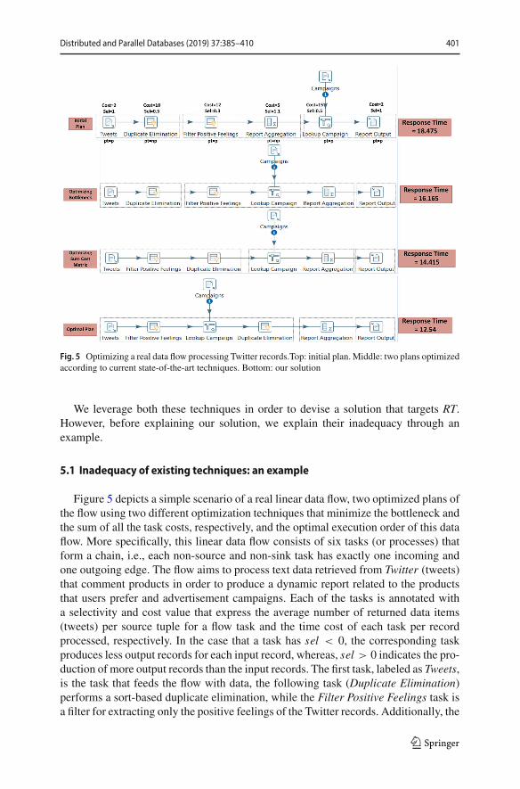
Fig. 5 Optimizing a real data flow processing Twitter records.Top: initial plan. Middle: two plans optimizedaccording to current state-of-the-art techniques. Bottom: our solution

We leverage both these techniques in order to devise a solution that targets RT.However, before explaining our solution, we explain their inadequacy through anexample.

5.1 Inadequacy of existing techniques: an example

Figure 5 depicts a simple scenario of a real linear data flow, two optimized plans ofthe flow using two different optimization techniques that minimize the bottleneck andthe sum of all the task costs, respectively, and the optimal execution order of this dataflow. More specifically, this linear data flow consists of six tasks (or processes) thatform a chain, i.e., each non-source and non-sink task has exactly one incoming andone outgoing edge. The flow aims to process text data retrieved from Twitter (tweets)that comment products in order to produce a dynamic report related to the productsthat users prefer and advertisement campaigns. Each of the tasks is annotated witha selectivity and cost value that express the average number of returned data items(tweets) per source tuple for a flow task and the time cost of each task per recordprocessed, respectively. In the case that a task has sel < 0, the corresponding taskproduces less output records for each input record, whereas, sel > 0 indicates the pro-duction of more output records than the input records. The first task, labeled as Tweets,is the task that feeds the flow with data, the following task (Duplicate Elimination)performs a sort-based duplicate elimination, while the Filter Positive Feelings task isa filter for extracting only the positive feelings of the Twitter records. Additionally, the

123


Report Aggregation is a task that produces reports, the Lookup Campaigns performsa lookup in a static data source to match each of the tweeted products with a set ofrelated campaigns for each product and finally, the Report Output task produces thefinal report. Based on their semantics, Duplicate Elimination and Report Aggregationare blocking tasks.

In the figure, we depict the initial plan and the results of the task ordering optimiza-tion when we target minimizing the bottleneck cost (according to the technique in[33]), the sum cost metric (according to the techniques in [17]) and the response time(this work). On the right, the response time per input record in each case is shown,where we see that the technique presented hereby (bottom plan) is capable of yieldingsignificant performance improvements. When calculating the response time, for sim-plicity, we assume that the α factor is set to 1. As such, RT is defined as the sum of themaximum task costs of each pipeline segment. The pipeline segments are delineatedby the dotted lines in the figure. During optimization, all dependency constraints arerespected; the constraints in this example define that Duplicate Elimination shouldalways precede Report Aggregation and, trivially, the source and the sink tasks shouldnot be moved.

The key lesson from this example is that when ordering the selective tasks by theircosts as in [33] or by their rank value, as in [17], neglecting the allocation of tasks topipeline segments, the overall response time may not be minimized.

5.2 Our solution

The basis of our solution is to split the initial flow into linear segments, each opti-mized individually. Algorithm 1 summarizes our approach.We first optimize the linearsub-flows using the best-performing technique in [17], called RO − I I I . This opti-mization is driven by the rank values, as explained above. Then, each linear sub-flowis decomposed into its pipelined segments.

For each such segment,we repeat a 3-phase process. In thefirst phase, inspiredby thework in [33], we order the tasks in away that the selective ones aremoved upstream andtheir relative order is only by their cost. The check-moving operation in Algorithm1 is responsible for (i) checking whether the move does not violate the constraints inPC ; and (ii) running the simulator in Sect. 4 in order to establish as to whether themove is beneficial or not. In the second phase, the algorithm attempts to modify thepipelined segments in the same branch with a view to moving an expensive task ofone segment to an adjacent segment, when the cost of the expensive tasks is going tobe hidden due to overlapped execution. This type of optimization is exemplified in thebottom plan in Fig. 5. Since the second step may have modified the contents of thepipelined segments, in the third phase we repeat the process of the first phase.

Two main features of this solution are: (i) By its design, it cannot yield worse plansin terms of RT than RO-III; i.e., our solutions either retains the solution of RO-III orproduces a faster plan. (ii) The optimization is machine-type specific, since it heavilyrelies on the simulator in Sect. 4, which is parameterized by the machine type-specificα factors (see also the algorithm input). This implies that it must be repeated for thesame flow when the execution engine host is modified. In practice, the optimization

123


Algorithm 1 Task re-ordering for optimizing RTInput: G(V , E), PC(V , E), ci , seli , pti ∀ti , α(p), p = 1 . . . |V |

split flow into linear branchesfor each branch Glinear (V , E) and its corresponding PC(V , D) do

plan P ← optimize Glinear for SCM − F using the RO − I I I algorithm in [17]

//Phase-Iidentify pipelined segment boundaries in P (i.e., tasks with pt = np)for each pipelined segment SP (sub-flow of P) do

for i in 1 …size(SP) dotbest ← the task after position i with sel < 1 and the lowest costif ∃tbest then

check-moving tbest to position i and shift other tasks to the right

//Phase-IIfor each pipelined segment SP (sub-flow of P) do

for i in 1 …size(SP) docheck-moving t in position i at the beginning of the next SP

for each pipelined segment SP (sub-flow of P) dofor i in 1 …size(SP) do

check-moving t in position i at the end of the previous SP

//Phase-IIIRepeat Phase-I

time is dominated by RO − I I I and the list scheduler simulator, but is negligible inmachines, such as those used in Sect. 4, i.e., it does not exceed a few seconds, evenfor flows of 24 tasks.

5.2.1 Analysis

Let a flow with n tasks and its largest linear sub-flow containing nl tasks. Extractinglinear sub-flows and applying RO-III to each such sub-flow takes O(n) and O(n2l )time, respectively [17]. check-moving is an O(n2) process regarding checkingviolations of the dependencies and O(n) to estimate RT through simulation. In theworst case, the nested loop in Phase-I in Algorithm 1 is repeated nl times. Therefore,the complexity of Phase-I is O(nln2) = O(n3). Similarly, the complexity of thenext two phases is also O(n3). Overall, our solution is of cubic complexity, which ispractical for very large flows of 100-200 tasks.

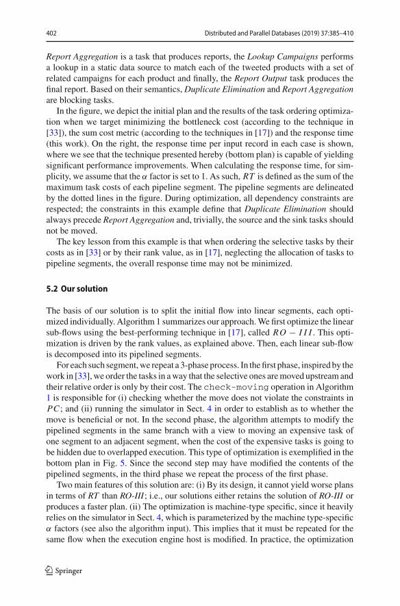
6 Evaluation of the response time optimizations

In the initial set of experiments, we focus on linear flows and we conduct a thoroughevaluation varying three dimensions: (i) the number of tasks in the flow; (ii) the per-centage of the edges in PC(V , D) compared to the case that D is a complete graph;and (iii) the percentage of blocking operators. The higher the percentage of PC edgesis, the less flexibility in re-ordering tasks exists. Also, the higher the percentage ofblocking operators, the higher the number of pipelined segments in the flow. For each

123


8/25

/25

8/25

/50

8/25

/75

8/50

/25

8/50

/50

8/50

/75

8/75

/25

8/75

/50

8/75

/75

16/2

5/25

16/2

5/50

16/2

5/75

16/5

0/25

16/5

0/50

16/5

0/75

16/7

5/25

16/7

5/50

16/7

5/75

24/2

5/25

24/2

5/50

24/2

5/75

24/5

0/25

24/5

0/50

24/5

0/75

24/7

5/25

24/7

5/50

24/7

5/75

n/ PCs/ % blocking tasks

0

5

10

15

20

25

5-10%>10%

Fig. 6 Percentage of cases in which our solutions yielded lower RT than RO-III by at least 5%

dimension, we examined three values: 8, 16 and 24 tasks, and 25%, 50% and 75% forthe two percentages. Overall, we investigated 33 = 27 combinations. Each combina-tion is simulated 200 times, with the a factor being the same as the one in Fig. 3(top).In each run, we assigned random values to the cost and selectivity task metadata; thecost ranged from 1 to 100, and the selectivity ranged from 0.01 to 1.5.

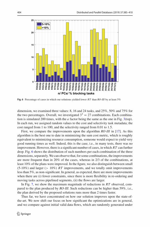
First, we compare the improvements upon the algorithm RO-III in [17]. As thisalgorithm is the best one to date in minimizing the sum cost metric, which is roughlyequivalent to minimizing resource consumption, someone would expect to yield verygood running times as well. Indeed, this is the case, i.e., in many tests, there was noimprovement. However, there is a significant number of cases, inwhich RT can furtherdrop. Fig. 6 shows the distribution of such numbers per each combination of the threedimensions, separately.Wecanobserve that, for somecombinations, the improvementsare more frequent than in 20% of the cases, whereas in 2/3 of the combinations, atleast 10% of the plans were improved. In the figure, we also distinguish between small(5-10%) and larger (> 10%) RT improvements, and we totally omit improvementsless than 5%, as non-significant. In general, as expected, there are more improvementswhen there are (i) fewer constraints, since there is more flexibility in re-ordering andmoving tasks across pipelined segments, (ii) the flows are larger.

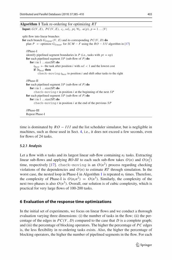
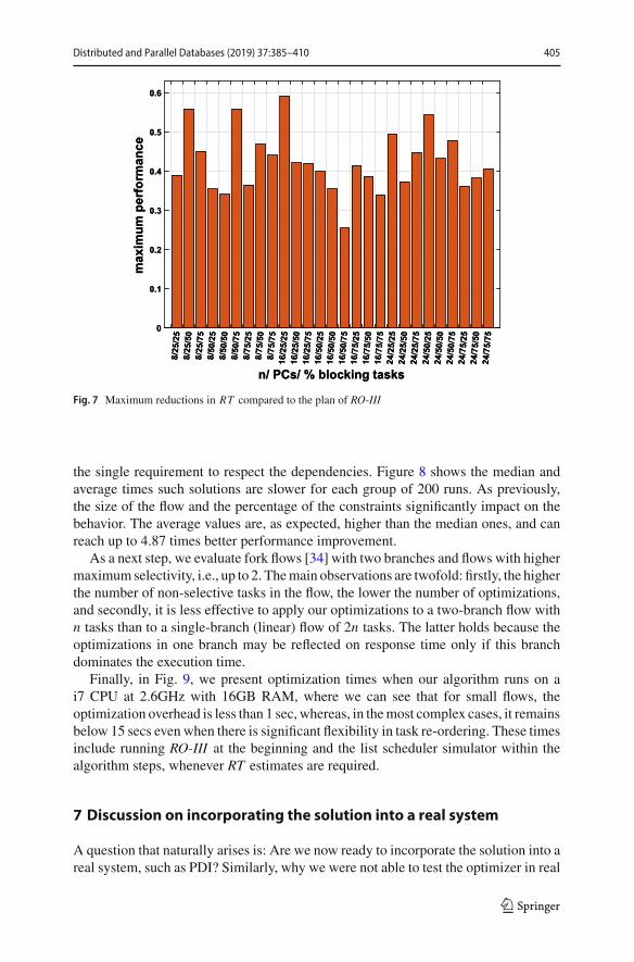
In Fig. 7, we show the maximum magnitude of reductions in RT observed, com-pared to the plan produced by RO-III. Such reductions can be higher than 59%, i.e.,the plan derived by the proposed solutions runs more than 2 times faster.

Thus far, we have concentrated on how our solution improves upon the state-of-the-art. We now shift our focus on how significant the optimizations are in general,and we compare against initial valid data flows, which are randomly generated under

123


8/25

/25

8/25

/25

8/25

/50

8/25

/50

8/25

/75

8/25

/75

8/50

/25

8/50

/25

8/50

/50

8/50

/50

8/50

/75

8/50

/75

8/75

/25

8/75

/25

8/75

/50

8/75

/50

8/75

/75

8/75

/75

16/2

5/25

16/2

5/25

16/2

5/50

16/2

5/50

16/2

5/75

16/2

5/75

16/5

0/25

16/5

0/25

16/5

0/50

16/5

0/50

16/5

0/75

16/5

0/75

16/7

5/25

16/7

5/25

16/7

5/50

16/7

5/50

16/7

5/75

16/7

5/75

24/2

5/25

24/2

5/25

24/2

5/50

24/2

5/50

24/2

5/75

24/2

5/75

24/5

0/25

24/5

0/25

24/5

0/50

24/5

0/50

24/5

0/75

24/5

0/75

24/7

5/25

24/7

5/25

24/7

5/50

24/7

5/50

24/7

5/75

24/7

5/75

n/ PCs/ % blocking tasksn/ PCs/ % blocking tasks

00

0.10.1

0.20.2

0.30.3

0.40.4

0.50.5

0.60.6

max

imum

per

form

ance

max

imum

per

form

ance

Fig. 7 Maximum reductions in RT compared to the plan of RO-III

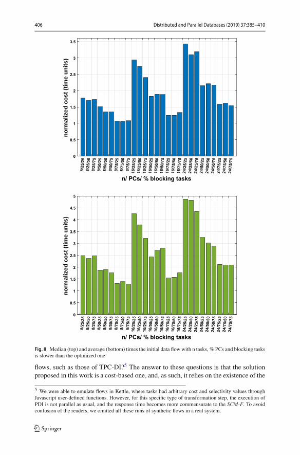
the single requirement to respect the dependencies. Figure 8 shows the median andaverage times such solutions are slower for each group of 200 runs. As previously,the size of the flow and the percentage of the constraints significantly impact on thebehavior. The average values are, as expected, higher than the median ones, and canreach up to 4.87 times better performance improvement.

As a next step, we evaluate fork flows [34] with two branches and flows with highermaximum selectivity, i.e., up to 2. Themain observations are twofold: firstly, the higherthe number of non-selective tasks in the flow, the lower the number of optimizations,and secondly, it is less effective to apply our optimizations to a two-branch flow withn tasks than to a single-branch (linear) flow of 2n tasks. The latter holds because theoptimizations in one branch may be reflected on response time only if this branchdominates the execution time.

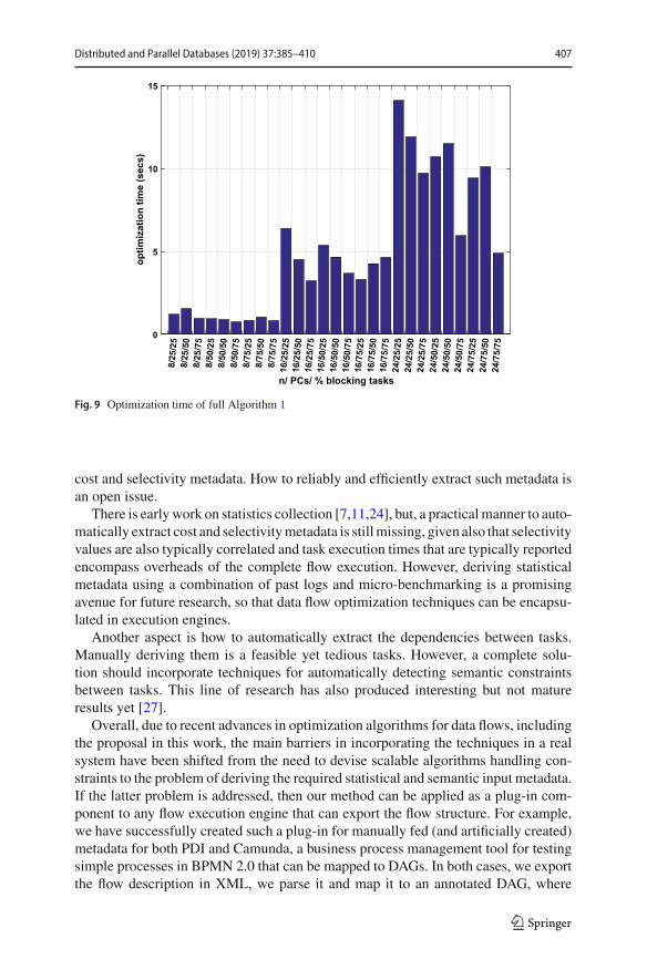
Finally, in Fig. 9, we present optimization times when our algorithm runs on ai7 CPU at 2.6GHz with 16GB RAM, where we can see that for small flows, theoptimization overhead is less than 1 sec, whereas, in themost complex cases, it remainsbelow 15 secs even when there is significant flexibility in task re-ordering. These timesinclude running RO-III at the beginning and the list scheduler simulator within thealgorithm steps, whenever RT estimates are required.

7 Discussion on incorporating the solution into a real system

A question that naturally arises is: Are we now ready to incorporate the solution into areal system, such as PDI? Similarly, why we were not able to test the optimizer in real

123


8/25

/25

8/25

/50

8/25

/75

8/50

/25

8/50

/50

8/50

/75

8/75

/25

8/75

/50

8/75

/75

16/2

5/25

16/2

5/50

16/2

5/75

16/5

0/25

16/5

0/50

16/5

0/75

16/7

5/25

16/7

5/50

16/7

5/75

24/2

5/25

24/2

5/50

24/2

5/75

24/5

0/25

24/5

0/50

24/5

0/75

24/7

5/25

24/7

5/50

24/7

5/75


0

0.5

1

1.5

2

2.5

3

3.5

norm

aliz

ed c

ost (

time

units

)

8/25

/25

8/25

/50

8/25

/75

8/50

/25

8/50

/50

8/50

/75

8/75

/25

8/75

/50

8/75

/75

16/2

5/25

16/2

5/50

16/2

5/75

16/5

0/25

16/5

0/50

16/5

0/75

16/7

5/25

16/7

5/50

16/7

5/75

24/2

5/25

24/2

5/50

24/2

5/75

24/5

0/25

24/5

0/50

24/5

0/75

24/7

5/25

24/7

5/50

24/7

5/75


0

0.5

1

1.5

2

2.5

3

3.5

4

4.5

5

norm

aliz

ed c

ost (

time

units

)

Fig. 8 Median (top) and average (bottom) times the initial data flow with n tasks, % PCs and blocking tasksis slower than the optimized one

flows, such as those of TPC-DI?5 The answer to these questions is that the solutionproposed in this work is a cost-based one, and, as such, it relies on the existence of the

5 We were able to emulate flows in Kettle, where tasks had arbitrary cost and selectivity values throughJavascript user-defined functions. However, for this specific type of transformation step, the execution ofPDI is not parallel as usual, and the response time becomes more commensurate to the SCM-F. To avoidconfusion of the readers, we omitted all these runs of synthetic flows in a real system.

123


8/25

/25

8/25

/50

8/25

/75

8/50

/25

8/50

/50

8/50

/75

8/75

/25

8/75

/50

8/75

/75

16/2

5/25

16/2

5/50

16/2

5/75

16/5

0/25

16/5

0/50

16/5

0/75

16/7

5/25

16/7

5/50

16/7

5/75

24/2

5/25

24/2

5/50

24/2

5/75

24/5

0/25

24/5

0/50

24/5

0/75

24/7

5/25

24/7

5/50

24/7

5/75


0

5

10

15

optim

izat

ion

time

(sec

s)

Fig. 9 Optimization time of full Algorithm 1

cost and selectivity metadata. How to reliably and efficiently extract such metadata isan open issue.

There is earlywork on statistics collection [7,11,24], but, a practicalmanner to auto-matically extract cost and selectivitymetadata is stillmissing, given also that selectivityvalues are also typically correlated and task execution times that are typically reportedencompass overheads of the complete flow execution. However, deriving statisticalmetadata using a combination of past logs and micro-benchmarking is a promisingavenue for future research, so that data flow optimization techniques can be encapsu-lated in execution engines.

Another aspect is how to automatically extract the dependencies between tasks.Manually deriving them is a feasible yet tedious tasks. However, a complete solu-tion should incorporate techniques for automatically detecting semantic constraintsbetween tasks. This line of research has also produced interesting but not matureresults yet [27].

Overall, due to recent advances in optimization algorithms for data flows, includingthe proposal in this work, the main barriers in incorporating the techniques in a realsystem have been shifted from the need to devise scalable algorithms handling con-straints to the problem of deriving the required statistical and semantic input metadata.If the latter problem is addressed, then our method can be applied as a plug-in com-ponent to any flow execution engine that can export the flow structure. For example,we have successfully created such a plug-in for manually fed (and artificially created)metadata for both PDI and Camunda, a business process management tool for testingsimple processes in BPMN 2.0 that can be mapped to DAGs. In both cases, we exportthe flow description in XML, we parse it and map it to an annotated DAG, where

123


annotations correspond to metadata, we apply the optimizations and we transform itback to its native format.

8 Conclusions and future work

In this work, we address a limitation of existing data flow cost models that do not accu-rately estimate the response time of real data flow execution, which heavily dependson parallelism. We propose a model that considers the time overlaps during the taskexecution, while it is capable of quantifying the impact of concurrent task execution.The latter is an aspect largely overlooked to date and may lead to significant inac-curacies if neglected, e.g., we provided simple examples of deviations up to 50%.Additionally, we propose an optimization solution that aims to improve the responsetime of a data flow by defining the execution order of the flow tasks based on theproposed cost model. In our experiments, the proposed optimization technique hasshown to yield improvements of up to 59% compared to the state-of-the-art in dataflow task ordering.

Our work can be extended in two complementary ways. Firstly, to work towardsend-to-end solutions with a view to incorporating the techniques in a real system, asdiscussed in the previous section. Secondly, applying the proposed model relies onthe existence of accurate machine type-specific weight information; deriving efficientways to approximate the weights before flow execution and generalize over types ofexecution engine hosts is an open issue. Finally, another direction for future work isto make a deep dive into the low-level resource utilization and wait measurements toestablish the detailed cause of contention.

References

1. Agrawal, K., Benoit, A., Dufossé, F., Robert, Y.: Mapping filtering streaming applications with com-munication costs. In: SPAA, pp. 19–28 (2009)

2. Agrawal, K., Benoit, A., Dufossé, F., Robert, Y.: Mapping filtering streaming applications. Algorith-mica 62(1–2), 258–308 (2012)

3. Boehm, M., Tatikonda, S., Reinwald, B., Sen, P., Tian, Yuanyuan, Burdick, D.R., Vaithyanathan, S.:Hybrid parallelization strategies for large-scale machine learning in systemml. Proc. VLDB Endow.7(7), 553–564 (2014)

4. Burge, J., Munagala, K., Srivastava, U.: Ordering pipelined query operators with precedence con-straints. Technical Report 2005-40, Stanford InfoLab (2005)

5. Chaudhuri, S., Shim, Kyuseok: Optimization of queries with user-defined predicates. ACM Trans.Database Syst. 24(2), 177–228 (1999)

6. Chirkin, A.M, Belloum, A.S.Z., Kovalchuk, S.V., Makkes, M.X.: Execution time estimation for work-flow scheduling. WORKS ’14, pp. 1–10 (2014)

7. Chirkin A.M., Belloum, A.S.Z., Kovalchuk, S.V., Makkes, M.X.: Execution time estimation for work-flow scheduling. In: proceeding of the 9thWorkshop onWorkflows in Support of Large-Scale Science,pp. 1–10. IEEE Press (2014)

8. Deshpande, A., Hellerstein, L.: Parallel pipelined filter ordering with precedence constraints. ACMTransac. Algorithms 8(4), 41:1–41:38 (2012)

9. DeWitt, D.J., Gray, J.: Parallel database systems: The future of high performance database systems.Commun. ACM, 35(6) (1992)

123


10. Florescu, D., Levy, A., Manolescu, I., Suciu, D.: Query optimization in the presence of limited accesspatterns. In: Proceedings of the 1999ACMSIGMOD international conference onManagement of data,SIGMOD ’99, pp. 311–322. ACM (1999)

11. Halasipuram, R., Deshpande, P.M., Padmanabhan, S.: Determining essential statistics for cost basedoptimization of an ETL workflow. In EDBT, pp. 307–318 (2014)

12. Hellerstein, J.M.: Optimization techniques for queries with expensive methods. ACM Trans. DatabaseSyst. 23(2), 113–157 (1998)

13. Hueske, F., Peters, M., Sax, M., Rheinländer, A., Bergmann, R., Krettek, A., Tzoumas, K.: Openingthe black boxes in data flow optimization. PVLDB 5(11), 1256–1267 (2012)

14. Ibaraki, T., Kameda, T.: On the optimal nesting order for computing n-relational joins. ACM Trans.Database Syst. 9(3), 482–502 (1984)

15. Kougka, G., Gounaris, A.: On optimizing workflows using query processing techniques. In: SSDBM,pp. 601–606 (2012)

16. Kougka,G.,Gounaris,A.:Optimization of data-intensiveflows: is it needed? is it solved? In: proceedingof the DOLAP, pp.95–98 (2014)

17. Kougka, G., Gounaris, A.: Cost optimization of data flows based on task re-ordering. T. Large-ScaleData- and Knowledge-Centered Systems 33, pp. 113–145 (2017)

18. Kougka, G., Gounaris, A.: Optimal task ordering in chain data flows: exploring the practicality of non-scalable solutions. In Big Data Analytics and Knowledge Discovery-19th International Conference,DaWaK 2017, Lyon, August 28-31, 2017, Proceedings, pp. 19–32 (2017)

19. Kougka, G., Gounaris, A., Leser: Ulf Modeling data flow execution in a parallel environment. In: BigData Analytics and Knowledge Discovery-19th International Conference, DaWaK 2017, pp. 183–196(2017)

20. Kougka, G., Gounaris, A., Simitsis, A.: The many faces of data-centric workflow optimization: asurvey. International Journal of Data Science and Analytics (2018)

21. Krishnamurthy, R., Boral, H., Zaniolo, C.: Optimization of nonrecursive queries. In: VLDB, pp. 128–137 (1986)

22. Kumar, N., Kumar, P.S.: An efficient heuristic for logical optimization of ETL workflows. In: BIRTE,pp.68–83 (2010)

23. Pietri, I., Juve, G., Deelman, E., Sakellariou, R.: A performance model to estimate execution time ofscientific workflows on the cloud. WORKS ’14, pp. 11–19. IEEE Press (2014)

24. Pietri, I., Juve, G., Deelman, E., Sakellariou, R.: A performance model to estimate execution time ofscientific workflows on the cloud. In: Proceeding of the 9th Workshop on Workflows in Support ofLarge-Scale Science, pp. 11–19. IEEE Press (2014)

25. Poess, M., Rabl, T., Caufield, B.: TPC-DI: the first industry benchmark for data integration. PVLDB7(13), 1367–1378 (2014)

26. Rheinländer, A., Heise, A., Hueske, F., Leser, U., Naumann, Felix: SOFA: an extensible logical opti-mizer for UDF-heavy data flows. Inf. Syst. 52, 96–125 (2015)

27. Rheinländer, A., Leser, U., Graefe, G.: Optimization of complex dataflowswith user-defined functions.ACM Comput. Surv. 50(3), 38:1–38:39 (2017)

28. Rheinländer, A., Heise, A., Hueske, F., Leser, U., Naumann, F.: Sofa: An extensible logical optimizerfor udf-heavy data flows. Inform. Syst. 52, 96–125 (2015)

29. Shi, J., Zou, J., Jiaheng, L., Cao, Z., Li, S., Wang, C.: Mrtuner: a toolkit to enable holistic optimizationfor mapreduce jobs. Proc. VLDB Endow. 7(13), 1319–1330 (2014)

30. Simitsis, A., Vassiliadis, P., Sellis, T.K.: State-space optimization of ETL workflows. IEEE Trans.Knowl. Data Eng. 17(10), 1404–1419 (2005)

31. Simitsis, A.,Wilkinson, K., Dayal, U., Castellanos,M.: Optimizing ETLworkflows for fault-tolerance.In: ICDE, pp. 385–396 (2010)

32. Singhal, R., Verma, A.: Predicting job completion time in heterogeneous mapreduce environments. In:IEEE IPDPSW, pp. 17–27 (2016)

33. Srivastava, U., Munagala, K., Widom, J., Motwani, R.: Query optimization over web services. In:Proceeding of the PVLDB, pp. 355–366 (2006)

34. Tziovara V., Vassiliadis, P., Simitsis, A.: Deciding the physical implementation of ETL workflows. In:DOLAP, pp. 49–56 (2007)

35. Verma, A., Cherkasova, L., Roy, H.: Campbell. Aria: Automatic resource inference and allocation formapreduce environments. ICAC ’11, pp. 235–244. ACM (2011)

123


36. Yerneni, R. , Li, C., Ullman, J.D., Garcia-Molina, Hector: Optimizing large join queries in mediationsystems. In: ICDT, pp. 348–364 (1999)

37. Zhang, Z., Cherkasova, L., Loo, BT.: Performancemodeling ofmapreduce jobs in heterogeneous cloudenvironments. CLOUD ’13, pp. 839–846 (2013)

Publisher’s Note Springer Nature remains neutral with regard to jurisdictional claims in published mapsand institutional affiliations.

123

Documents

Optimization of data flow execution in a parallel environment