Optimization of Collection System Maintenance Frequencies ... · Optimization of Collection System Maintenance Frequencies and System Performance Prepared by Black & Veatch LLP for

OPTIMIZATION OF COLLECTIONSYSTEM MAINTENANCE FREQUENCIES

AND SYSTEM PERFORMANCE

American Society of Civil EngineersEPA Cooperative Agreement #CX 824902-01-0

February 1999

Optimization of Collection System Maintenance Frequencies and System Performance

Prepared

by

Black & VeatchLLP

for

American Society of Civil Engineers

Under

Cooperative Agreement

with

U.S. Environmental Protection AgencyOffice of Wastewater Management

Washington, DC

EPA Cooperative Agreement #CX 824902-01-0February 1999

NOTICE

The material in this document has been subject to U.S. Environmental

Protection Agency technical and policy review and approved for

publication. The views expressed by individual authors, however, are their

own and do not necessarily reflect those of the U.S. Environmental

Protection Agency

Table of Contents

Page No.

i

Acknowledgements................................................................................................................ vii

Executive Summary .................................................................................................................1

1.0 Introduction and Background..........................................................................................1-11.1 Project Significance and Objectives ........................................................................1-11.2 Background .........................................................................................................1-21.3 Review of Literature.............................................................................................1-21.4 Relationship of System Performance and Reinvestment ............................................1-31.5 Theory................................................................................................................1-31.6 Perceived Effectiveness of Existing Maintenance Programs.......................................1-51.7 Statistical Analyses Performed ...............................................................................1-71.8 Benefits...............................................................................................................1-71.9 Report Organization..............................................................................................1-71.10 Abbreviations and Definitions.................................................................................1-8

2.0 Data Collection..............................................................................................................2-12.1 Development of Questionnaire ...............................................................................2-12.2 Identification of Participants ..................................................................................2-32.3 Data Collection.....................................................................................................2-4

3.0 Agency Data.................................................................................................................3-13.1 Introduction.........................................................................................................3-13.2 Service Area Characteristics ..................................................................................3-1

3.2.1 Summary of Service Area Information........................................................3-13.3 Flow Information .................................................................................................3-6

3.3.1 Summary of Flow Information ..................................................................3-63.4 Information on System Characteristics ...................................................................3-8

3.4.1 Summary of Characteristic Information ......................................................3-84.0 Maintenance Data..........................................................................................................4-1

4.1 Introduction.........................................................................................................4-14.2 Routine Maintenance.............................................................................................4-14.3 Inspection Maintenance.........................................................................................4-54.4 Rehabilitation Maintenance.....................................................................................4-84.5 System Maintenance Costs....................................................................................4-9

5.0 System Maintenance Frequency Determination .................................................................5-15.1 Introduction.........................................................................................................5-15.2 Weighting of Maintenance Activities .......................................................................5-15.3 Development of Maintenance Frequency.................................................................5-2

5.3.1 Determining Maintenance Rates .................................................................5-25.3.2 Developing the Standard Rating..................................................................5-3

Determination of Maintenance Frequency.........................................................................5-85.5 Performance Indicators.......................................................................................5-105.6 Regression Analysis for Maintenance Frequency....................................................5-10Conclusions ................................................................................................................5-14

Table of Contents (Continued)

Page No.

ii

6.0 Determination of System Performance Rating...................................................................6-16.1 Introduction.........................................................................................................6-16.2 Performance Data Weighting .................................................................................6-16.3 Development of Performance Rating ......................................................................6-2

6.3.1 Determining Performance Rating................................................................6-36.3.2 Developing the Standard Rating..................................................................6-3

6.4 Determination of Performance Rating .....................................................................6-86.4.1 Annual Reinvestment ..............................................................................6-106.4.2 Regression Analysis for Performance Rating .............................................6-11

6-5 Estimates of Reinvestment...................................................................................6-146-6 Conclusion ........................................................................................................6-16

7.0 Optimizing Collection System Maintenance.......................................................................7-17.1 Introduction.........................................................................................................7-17.2 Collection System Maintenance Frequency..............................................................7-17.3 Performance Rating..............................................................................................7-5

7.3.1 Establish Performance Rating ....................................................................7-57.4 Determine Historical Reinvestment Rate ..................................................................7-87.5 Optimizing Collection System Maintenance............................................................7-12

7.5.1 Optimization Of Maintenance For an Agency.............................................7-127.5.2 Optimizing Maintenance for Agency No. 42 ..............................................7-13

7.6 Conclusion ........................................................................................................7-177.7 Recommendations ..............................................................................................7-17

List of Tables

Page No.

iii

Table 2-1 Questionnaire Matrix ...........................................................................................2-2Table 2-2 System Size and Population Classification..............................................................2-4Table 2-3 Summary of Agencies by Size and Region .............................................................2-1Table 3-1 Summary of System Characteristics .....................................................................3-2Table 3-2 Sewer Density....................................................................................................3-3Table 3-3 Percentage of System vs. Average Age .................................................................3-5Table 3-4 ADF vs. Population.............................................................................................3-7Table 3-5 Peak Hourly/ADF................................................................................................3-8Table 3-6 Percentage of System Greater than 24 Inches in Diameter .......................................3-9Table 3-7 Number of Pump Stations....................................................................................3-9Table 3-8 Total Installed Horsepower of Pump Stations .......................................................3-10Table 3-9 Ration-Force Main Length/Pump Station .............................................................3-10Table 3-10 Percentage of System Industrial/Commercial Flow ...............................................3-11Table 3-11 Typical Velocity of Flow ...................................................................................3-11Table 4-1 Routine Maintenance - Average Sewer 5-Year Cleaning...........................................4-2Table 4-2 Routine Maintenance - Average Root Removal .......................................................4-2Table 4-3 Routine Maintenance - Average Main Line Stoppages Cleared ..................................4-3Table 4-4 Routine Maintenance - Average House Service Stoppages Cleared ............................4-4Table 4-5 Routine Maintenance - Average Inspections & Service of Pump Stations ..................4-4Table 4-6 Inspection Methods - Flow Evaluation...................................................................4-5Table 4-7 Inspection Methods - Manhole Inspection..............................................................4-6Table 4-8 Inspection Methods - Smoke/Dye Testing .............................................................4-7Table 4-9 Inspection Methods - Television Inspection ...........................................................4-7Table 4-10 Inspection Methods - Private Sector Building Inspection .........................................4-8(Table 4-11 Rehabilitation Maintenance Status .........................................................................4-9Table 4-12 Relief Maintenance Costs by Period ....................................................................4-10Table 4-13 Equalization Costs.............................................................................................4-10Table 4-14 Rehabilitation/Replacement Costs by Period .........................................................4-10Table 4-15 O&M Budget by Period .....................................................................................4-11Table 4-16 Rate of Spending ..............................................................................................4-11Table 5-1 Average Weight of Maintenance Activity ...............................................................5-2Table 5-2 Maintenance Performed.......................................................................................5-4Table 5-3 Reported Maintenance Rates ................................................................................5-5Table 5-4 Maintenance Activity Statistics .............................................................................5-6Table 6.5 Standardized Maintenance Frequency Table by Maintenance Rate.............................5-7Table 5-6 Calculated Maintenance Frequencies .....................................................................5-9Table 5-7 Range and Mean of System Maintenance Frequencies ...........................................5-10Table 5-8 Potential Independent Variables Related to Maintenance Frequency.........................5-12Table 5-9 Regression Analysis for Maintenance Frequency ..................................................5-13Table 5-10 Regression Coefficients for Maintenance Frequencies ...........................................5-13

List of Tables (Continued)

Page No.

iv

Table 6-1 Performance Measure Weight ..............................................................................6-2Table 6-2 Utility Performance Data......................................................................................6-4Table 6-3 Performance Rates..............................................................................................6-5Table 6-4 Performance Data Statistics .................................................................................6-6Table 6-5 Standardized Performance Rating Table by Performance Measure............................6-7Table 6-6 Calculated Performance Ratings ...........................................................................6-9Table 6-7 Summary of Performance Rating Derived............................................................6-10Table 6-8 Agency Reinvestment Data ................................................................................6-12Table 6-9 Potential Independent Variables Related to Performance Rating ..............................6-12Table 6-10 Regression Analysis for Performance Ratios ........................................................6-13Table 6-11 Regression Coefficients for Performance Rating...................................................6-13Table 6-12 Regression Analysis for Reinvestment .................................................................6-15Table 6-13 Regression Coefficients for Reinvestment............................................................6-15Table 7-1 Activities for Determination of Maintenance Frequencies .........................................7-2Table 7-2 Normalized Maintenance Frequency for Given Maintenance Activity Rate .................7-3Table 7-3 Activity Weighting Factor ....................................................................................7-4Table 7-4 Performance Measure and Units ...........................................................................7-5Table 7-5 Normalized Performance Rates for Given Performance Measure Values....................7-7Table 7-6 Performance Weighting Factor.............................................................................7-8Table 7-7 Determination of Reinvestment.............................................................................7-8Table 7-8 Reinvestment Regression Coefficients .................................................................7-10Table 7-9 Actual and Predicted Reinvestment Rates.............................................................7-12Table 7-10 Determination of Maintenance Frequency for Agency No. 42 ................................7-14Table 7-11 Determination of Performance Rating for Agency No. 42......................................7-15Table 7-12 Determination of Reinvestment...........................................................................7-16

List of Figures

Page No.

v

Figure 1-1 System Value and System Age (No Rehabilitation)..................................................1-4Figure 1-2 System Value and System Age (With Rehabilitation) ...............................................1-4Figure 1-3 System Performance and Maintenance Frequency..................................................1-5Figure 1-4 Perceived Satisfaction with Existing Maintenance Program......................................1-6Figure 2-1 Date Collection Services by Region and Size ..........................................................2-5Figure 3-1 Sewer Miles vs. Population ..................................................................................3-3Figure 3-2 Area Served vs. Sewer Miles................................................................................3-4Figure 3-3 Average Age by Agency ......................................................................................3-5Figure 3-4 Cumulative System Length by Average Age (Years)................................................3-6Figure 3-5 ADF vs. Population.............................................................................................3-7Figure 5-1 Maintenance Frequency Assignments....................................................................5-8Figure 5-2 Collection System Maintenance Frequency Distribution.........................................5-10Figure 5-3 Calculated vs. Predicted Maintenance Frequency..................................................5-14Figure 6-1 Assignment of Performance Rating.......................................................................6-8Figure 6-2 Collection System Weighted Performance Rating..................................................6-10Figure 6-3 Predicted Versus Measured Performance Rating...................................................6-14Figure 6-4 Predicted Versus Actual $/mi�yr........................................................................6-16Figure 7-1 Estimated Desirable System Performance and Reinvestment Envelope ....................7-11Figure 7-2 Estimated Target Envelope for Performance Rating and Maintenance Frequency......7-13

Appendices

vi

Appendix A: Questionnaire

Appendix B: Data Provided by Respondents

Appendix C: Maintenance Activities Weighting

Appendix D: Collection System Performance Weighting

Appendix E: Liteature Review

Appendix F: Optimization of Collection System Maintenance Frequencies and System Performance (with sample diskette)

vii

Acknowledgments

The authors of this report wish to thank the United States Environmental Protection Agency

(USEPA), Black & VeatchLLP, and the American Society of Civil Engineers (ASCE) for their

support of this study. The authors acknowledge the critical input provided by the members of the

Technical Advisory Committee (TAC).

Authors

Richard E. NelsonPrincipal Investigator

Black & VeatchLLP

8400 Ward ParkwayP.O. Box 8045Kansas City, MO 64114

(913)[email protected]

Paul H. Hsiung Black & VeatchLLP



Aaron A. Witt Black & VeatchLLP



Technical Advisory Committee (TAC)Joseph W. Barsoom Wastewater Management Division

City and County of Denver2000 W. 3rd AvenueDenver, CO 80223


Carol W. Bowers ASCE1801 Alexander Bell DriveReston, VA 20191-4400


Ahmad Habibian Black & VeatchLLP

18310 Montgomery Village, Ave.Gaithersburg, MD 20879


Philip M. Hannan Washington Suburban Sanitary Commission14501 Sweitzer LaneLaurel, MD 20707


Kenneth D. Kerri California State University, Sacramento6000 J StreetSacramento, CA 95819-6025


John A. Redner County Sanitation Districts of Los Angeles County920 S. Alameda StreetCompton, CA 90221-4894

(310)638-1161 [email protected]

viii

EPA StaffBarry R. Benroth U.S. Environmental Protection Agency

401 M Street, SW, Mail Stop 4204Washington, DC 20460


Richard Field U.S. Environmental Protection AgencyBuilding 10, MS-1062890 Woodridge AvenueEdison, NJ 08537


Michael D. Royer U.S. Environmental Protection AgencyBuilding 10, MS-1042890 Woodridge AvenueEdison, NJ 08537


Kevin J. Weiss U.S. Environmental Protection Agency401 M Street, SWWashington, DC 20460

(202) [email protected]

Participating wastewater utilities and agencies provided needed information for this project

are listed below. Only those agencies granting permission to do so are listed by name.

Carpinteria Sanitary DistrictCarpinteria, CA

City of TulsaTulsa, Oklahoma

Charlotte-Mecklenburg Utilities, WastewaterCollectionCharlotte, NC

City of Wichita, Water and Sewer DepartmentWichita, KS

City of AlbuquerqueAlbuquerque, NM

Clark County Sanitation DistrictLas Vegas, NV

City of Columbus, Division of Sewerage andDrainageColumbus, OH

Columbia Sanitary Sewer UtilityColumbia, MO

City of Council Bluffs, Department of PublicWorksCouncil Bluffs, IA

Columbus Water WorksColumbus, GA

City of Dallas, Water Department, WastewaterCollection DivisionDallas, TX

County Sanitation Districts of Los Angeles CountyCompton, CA

City of DurhamDurham, NC

County of Sacramento, Public Works Agency,Water Quality Division, County Sanitation DistrictNo.1Sacramento, CA

City of FresnoFresno, CA

Little Rock, Wastewater UtilityLittle Rock, AR

City of GlendaleUtilities DepartmentGlendale, AZ

Madison Metropolitan Sewerage DistrictMadison, WI

ix

City of HoustonHouston, TX

Metropolitan Sewer District of Greater CincinnatiCincinnati, OH

City of Indianapolis, Department of Capital AssetManagementIndianapolis, IN

Metropolitan Council Environmental Services,Regional Maintenance FacilityEagan , OH

City of Kansas City, Water Service DepartmentKansas City, MO

Metropolitan St. Louis Sewer DistrictSt. Louis, MO

City of Las VegasLas Vegas, NV

Miami-Dade Water and Sewer DepartmentCoral Gables, FL

City of McMinnvilleMcMinnville, OR

Oklahoma City Water and Wastewater UtilitiesDepartmentOklahoma City, OK

City of ModestoModesto, CA

Pima County Wastewater Management DepartmentTucson, AZ

City of PhoenixPhoenix, AZ

Portland Water DistrictPortland, ME

City of Rochester, Department of Public WorksRochester, MN

Reedy Creek Energy Services, Inc.Reedy Creek Improvement DistrictLake Buena Vista, FL

City of ScottsdaleWater OperationsScottsdale, AZ

Unified Sewerage AgencyHillsboro, OR

City of Shreveport, Department of Water andSewerageShreveport,, LA

Washington Suburban Sanitary CommissionLaurel, MD

City of SpringfieldDepartment of Public WorksSpringfield, MO

Wastewater Management - City and County ofDenver, CO

Louisville & Jefferson County Metropolitan SewerDistrictLouisville, KY

1

Executive Summary

The objective of this project was to develop an optimized approach for maintenance of

separate collection systems. Maintenance has a broad definition as defined in this report, and

includes any reinvestment in an existing collection system in the form of cleaning, monitoring,

inspection, rehabilitation and relief. Hopefully, this project will benefit the general public, state and

local decision makers, and other potentially affected groups by reducing the failure rate of collection

systems. The reduction in the failure rate of collection systems will improve public health by

preventing sewer backups, and will also benefit the environment by minimizing discharge of

untreated sewage to surface waters. Specific objectives accomplished are as follows:

C the effectiveness of maintenance programs of agencies surveyed was evaluated byreviewing their maintenance activities and their frequency,

C a review of how maintenance and rehabilitation dollars spent are being spent,

C an overview of typical values for maintenance frequencies and system reinvestmentexpense amounts was performed to serve as benchmarks for local governmentsand agencies in evaluating their own programs, and

C guidelines and methods were developed to help agencies evaluate and Ameasure@their own maintenance frequency and performance rating by developing a singlenumber or Ayardstick@ which can be determined based on commonly collecteddata.

The wastewater collection system is a major capital investment, and agencies must ensure

they are providing safe and efficient service to their customers. The level of service, or system

performance, is difficult to quantify because of the many variables in collection systems.

Nevertheless, system performance can be improved and maintained at an acceptable level with

proper maintenance. This report provides guidance to answer the following questions: "How much

maintenance is enough?", AIs the performance of my system adequate and is it improving or getting

worse@ and "How do I determine the level of maintenance required?" Currently, there is no

rational approach for determining the frequencies of various maintenance procedures except

through experience and judgement.

Quality collection system maintenance consists of the optimum use of labor, equipment, and

materials to keep the system in good repair, so that it can efficiently accomplish its intended purpose

of collection and transportation of wastewater to the treatment plant. Serious health hazards and

2

extensive property damage can result from sanitary sewer backups and overflows. There should

be some reasonable balance between the cost of maintenance and the benefits derived.

The scope of work for this project included the following major task groups:

$ Task 1. Literature Search$ Task 2. Data Collection$ Task 3. Follow up and Data Compilation$ Task 4. Data Analysis$ Task 5. Report and Presentation

Very little data was identified in the literature search with respect to establishing

maintenance frequencies or performance ratings. This report then is a preliminary effort to develop

a rational approach to evaluating maintenance (reinvestment) and system performance. It is

expected that future studies will enhance and result in modifications to the approach presented

herein.

The data collection effort was somewhat protracted due to the amount of information

agencies were requested to provide and the difficulty of collecting the data needed. Most agencies

do not keep detailed records for all information requested and therefore the Abest guess@ was

provided in some instances. It is believed that the lack of quality data by many of the agencies

resulted in much of the scatter and broad range of data responses received. Nevertheless, it is also

believed that the data received support the hypothesis that performance and reinvestment are

related and that system performance and maintenance can be quantitatively evaluated to optimize

the system reinvestment for selected levels of system performance.

Based on the agency responses received cleaning, root removal, and pump station service

are the most important routine maintenance activities; although a total of 12 key maintenance

activities are still necessary for a balanced routine maintenance program. Using a statistical method

to develop a routine maintenance Ayard stick@, an average maintenance frequency, considering all

routine maintenance activities of 6.6% was derived with a range of 2.4% to 12.6%. The

relationship of maintenance and performance was explored and it was found that a strong

relationship exists between the maintenance frequency and system historical performance.

Independent variables related to maintenance frequency include customer complaints, manhole

overflows, pipe failures, system sizes, number of pump stations, regional location, and pump station

failures.

3

The agency responses received also identified pipe failures, SSOs, and customer

complaints as the most important performance measures. Using the same statistical method used

for establishing the maintenance yard stick, a performance yard stick was developed. Considering

all performance measures, an average performance rating of 71.1% was derived with a range of

53.1% to 97.2%. In addition to this performance rating, the amount of reinvestment was reviewed

and analyzed. It was found that the annual reinvestment has been increasing and for the period

1980 to 1996 has averaged $9,328/mi$yr or $1.77/ft$yr. The annual reinvestment for the life of

the systems as reported was about $1.00/ft$yr. These reinvestment rates support the theory of

reinvestment required presented in Chapter 1. The relationship between the performance rating and

reinvestment was explored and it was found that a strong relationship exists between these two

parameters.

Based on the methods developed for determining maintenance frequencies and

performance ratings, a method or approach for optimizing collection system maintenance is

presented with general guidance for the desirable envelope for performance and maintenance.

Collection system maintenance can be optimized by creating a better balance of maintenance

activities, increasing or decreasing budgets as appropriate, and evaluating performance of the

system against the maintenance frequency being implemented. In time, by monitoring both

maintenance and performance, agencies will be able to strike the right balance for their system and

maintain acceptable performance and the least reinvestment cost.

Because of the importance of system maintenance (reinvestment) and system performance,

it is recommended that ongoing research be performed to enhance and improve the work presented

in the report. Specific recommendations are as follows:

1. Review and refine the maintenance, performance, and reinvestment measures used in

this report. Develop detailed definitions of each.

2. Develop either an information collection guideline which would request agencies to

collect data consistent with Step 1 or have a study with a core group of agencies to

provide data that can be used to refine these analyses and to generate a AGuideline

Report for Collection System Maintenance.@

4

3. Implement the information collection process and use the data to develop cost

estimates, maintenance guidelines, and performance measures similar to those

presented in this study.

4. Repeat the analysis on a regular basis every 2 to 5 years as the output will improve with

the improved data collection.

1-1

1.0 Introduction and Background

Collection system maintenance and rehabilitation is being performed to meet regulatory

requirements and to improve sewerage service to customers. Maintenance as defined in this report

includes any reinvestment in an existing collection system in the form of cleaning, monitoring,

inspection, rehabilitation, and relief. Rehabilitation is performed to correct the deficiencies identified

from maintenance activities. With more emphasis being placed on maintenance, it is becoming

increasingly important to determine Ahow much maintenance is enough?@ According to the Water

Pollution Control Federation (WPCF) Manual of Practice No. 7, (1985), AThere should be some

reasonable balance between cost of preventive maintenance and benefit derived.@ This need is

demonstrated by a survey of 20 cities which showed a 1000-to-1 spread on main breaks and a

150-to-1 spread on stoppages per 1000 miles of sewer per year. Age and neglect were noted as

the primary reasons for these differences. (WEF 1994)

This study was undertaken to evaluate collection system maintenance and rehabilitation

needs based on information from a questionnaire completed by selected cities and agencies,

hereinafter referred to collectively as agencies. Specifically, the objectives were to evaluate the

effectiveness of maintenance programs by reviewing the inspection activities and their frequency;

to review how reinvestment dollars were spent; and to provide an overview of typical values to

serve as guidance for local governments and agencies in evaluating their own programs. It should

be noted that this study pertains to Aseparate@ collection systems only and does not include data for

combined sewer systems.

This project was performed by the American Society of Civil Engineers (ASCE) and Black

& VeatchLLP under a cooperative agreement with the U.S. Environmental Protection Agency

(USEPA).

1.1 Project Significance and Objectives

The objective of this project is to develop an approach for optimizing maintenance of

wastewater collection systems. The project will help wastewater agencies plan for maintenance

based on specific performance measures and will provide guidance on the total reinvestment

required to meet selected levels of system performance. Improved performance of collection

systems will benefit public health, and will also benefit the environment. This project presents a

1-2

decision making model which can be used by agencies in evaluating the cost of maintenance, as it

relates to maintenance frequency and system performance.

1.2 Background

Collection system maintenance is performed to meet regulatory requirements and to

improve sewerage service to customers. A collection system corrodes, erodes, collapses, clogs,

and ultimately deteriorates. Collection system capacity can be reduced by root growth; by the

accumulation of obstructions discharged to the system, such as grease, garbage, rags, paper towels,

and by structural failures such as line breaks and collapses. Maintenance, in the broad sense used

for this study, includes any reinvestment in an existing collection system in the form of cleaning,

monitoring, inspection activities, rehabilitation, and relief. Relief can be in the form of relief sewers,

additional pumping capacity or equalization facilities.

Wastewater collection systems are a major capital investment which agencies must properly

maintain to ensure safe and efficient service to their customers. The level of service, or system

performance, is difficult to quantify because of the many variables involved. Nevertheless, this

study attempts to develop an approach to measure system performance so that it can be monitored

and improved if necessary by proper maintenance procedures.

Many agencies have not provided the collection system maintenance necessary for an

adequate level of customer service and to protect the sizable investment in their facilities. We have

all heard the adage Aout of sight, out of mind@ as this relates to collection systems. Collection

system maintenance functions are frequently treated as a necessary evil, to be given attention only

as emergencies arise. Getting adequate maintenance budgets is dependent on justifying the level

of maintenance required. Currently, there is no rational approach to estimating the frequency of the

various maintenance procedures required, except through experience and judgment.

Quality collection system maintenance consists of the optimum use of labor, equipment, and

materials to keep the system in good condition so that it can efficiently accomplish its intended

purpose of collecting and transporting wastewater to the treatment plant. Serious health hazards

and extensive property damage can result from sanitary sewer backups and overflows. There

should be some reasonable balance between the cost of maintenance and the benefits derived.

1.3 Review of Literature

1-3

The authors of this project conducted an extensive literature search (see Appendix E,

Literature Review) to obtain nationwide information on current trends in collection system

maintenance planning. Very few publications were found that dealt with optimizing maintenance and

no publications were found that specifically addressed system maintenance frequency determination

or system performance rating evaluation. The literature contained very few papers on the subject

of collection system operation and maintenance. Most papers focused on engineering design or

sanitary sewer evaluation studies (SSES).

Details of the Literature review are contained in Appendix E.

1.4 Relationship of System Performance and Reinvestment

Collection system performance depends on regular and effective reinvestment. This study

explores the relationships between system performance, maintenance frequency, and reinvestment.

Without reinvestment and effective maintenance, collection systems will eventually fail.

1.5 Theory

The theoretical basis for establishing a relationship between system performance and

maintenance (reinvestment) is the hypothesis that collection systems deteriorate over time, with

consequent loss of system performance. To maintain system performance, ongoing reinvestment

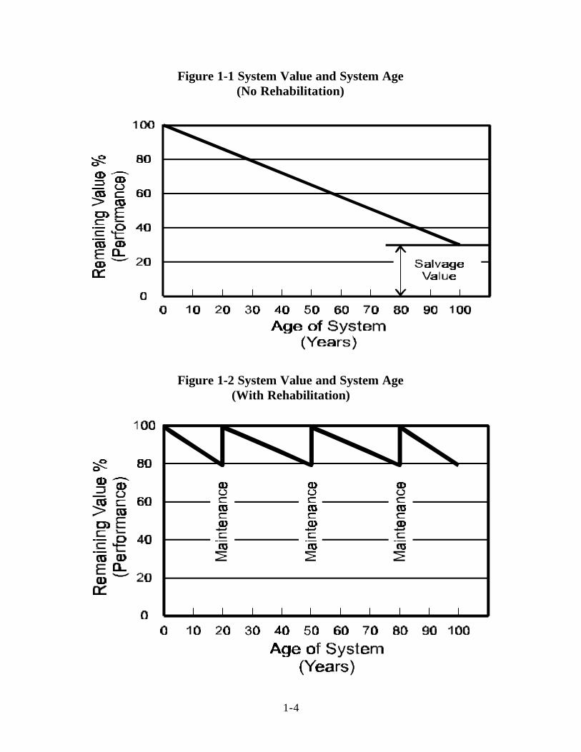
is required. For purposes of discussion, let us assume that the life of a sewer is 100 years, with 25

percent salvage value remaining at the end of the 100 years as shown on Figure 1-1. Furthermore,

we will assume an average system value of $100 per foot, or $528,000 per mile. Given these

assumptions, the rate of degradation would be $0.75 per year per foot of sewer system.

Next, let us assume that the life of a system can be extended past the 100 years through

system reinvestment in the form of rehabilitation, capital improvements, and routine maintenance.

A hypothetical cycle of degradation and maintenance is shown on Figure 1-2.

1-4

Figure 1-1 System Value and System Age(No Rehabilitation)

Figure 1-2 System Value and System Age(With Rehabilitation)

1-5

If complete maintenance (reinvestment) is performed each year, the system will operate at

100 percent efficiency all the time. If maintenance (reinvestment) is never performed, then the

system will degrade and perform at 25 percent of the efficiency of a new system after 100 years.

If maintenance (reinvestment) is performed at a rate of 2 percent per year, the system performance

will decrease to about 65 percent of a new system=s performance. If maintenance is performed at

4 percent per year, the minimum system performance would be about 80 percent; with maintenance

at 10 percent per year, the minimum performance would be about 93 percent of new system

performance. These scenarios are shown on Figure 1-3.

Figure 1-3 System Performance and Maintenance Frequency

This study researches relationships between system performance, maintenance rates, and

reinvestment. The objective, in concept, was to develop an approach similar to that depicted on

Figure 1-3, so that a desired maintenance frequency could be selected based on a minimum

acceptable performance rating for the system.

1.6 Perceived Effectiveness of Existing Maintenance Programs

Based on the survey responses obtained during this study, the effectiveness of existing

maintenance programs was evaluated. Each agency surveyed was asked the question, AAre you

satisfied with your system maintenance (total reinvestment) program?@ Each agency was requested

to respond with one of the following answers:

1-6

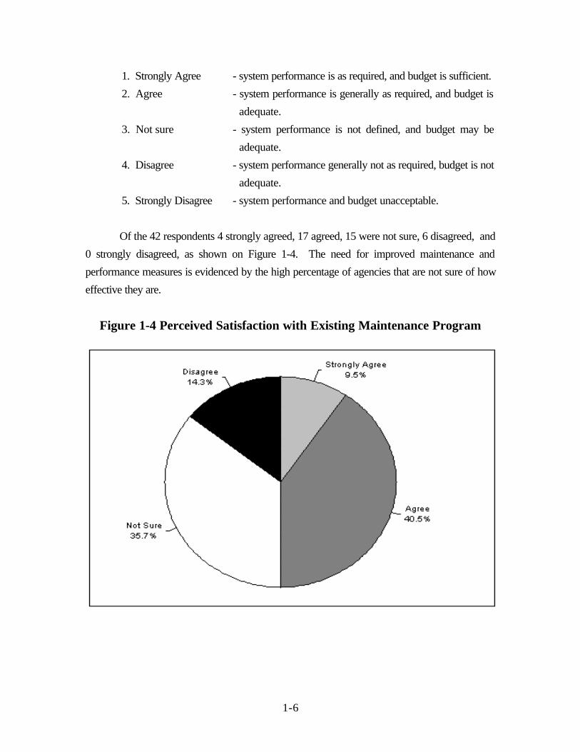
1. Strongly Agree - system performance is as required, and budget is sufficient.

2. Agree - system performance is generally as required, and budget is

adequate.

3. Not sure - system performance is not defined, and budget may be

adequate.

4. Disagree - system performance generally not as required, budget is not

adequate.

5. Strongly Disagree - system performance and budget unacceptable.

Of the 42 respondents 4 strongly agreed, 17 agreed, 15 were not sure, 6 disagreed, and

0 strongly disagreed, as shown on Figure 1-4. The need for improved maintenance and

performance measures is evidenced by the high percentage of agencies that are not sure of how

effective they are.

Figure 1-4 Perceived Satisfaction with Existing Maintenance Program

1-7

1.7 Statistical Analyses Performed

Statistical analyses were performed to evaluate data and data relationships. The analytical

methods include functions of random variables such as mean, variance, and standard deviations as

well as methods to evaluate relationships among independent variables in the form of linear

regression and multiple linear regression analyses. The SPSS 6.0 statistical software package for

Windows was employed for this purpose. The SPSS is a world leading statistical analysis software

package.

1.8 Benefits

The benefits derived from this report include guidance for measuring system maintenance,

system performance, and developing guidelines for reinvestment dollars. The methods developed

will help agencies evaluate the effectiveness of their current maintenance programs and establish

target performance goals. This study will also assist regulatory agencies in reviewing the

effectiveness of collection system maintenance programs and the adequacy of collection system

budgets which may result in environmental, economic, social, and public health improvements.

1.9 Report Organization

Chapter 1 describes the significance, objectives, background information on, and methods

used to evaluate collection systems performance. Chapter 2 introduces the criteria and measures

to be used in the evaluation of a collection system. Chapter 3 describes system characteristic data.

Chapter 4 describes the system performance data. The measures associated with each criterion,

the determination of maintenance frequency and performance rating are discussed in Chapters 5

and 6. Comprehensive performance evaluations are also discussed. Chapter 7 presents the use

of these tools for optimizing collection system maintenance. Supplemental data , overview of

relevant literature regarding collection system performance and maintenance, and the survey form

are presented in the appendices.

1-8

1.10 Abbreviations and Definitions

Abbreviations

#ps/mi number of pump stations per mile of sewer$/mi$yr cost per mile of sewer per year$/ft$yr cost per foot of sewer per year%/system$yr percent of sewer system per yearADF average annual daily flowASCE American Society of Civil Engineersavg average (mean)CCTV closed circuit TVfm/ps miles of forcemain per pump stationfps feet per secondgpcd gallons per capita per dayhp horsepowerhp/mi horsepower per mile of sewerI/I inflow/infiltrationkWh kilowatts per hourps/mi pump stations per milemax maximum valuemgd million gallons per daymin minimum valueno/ps$yr number per pump station per yearno/mi$yr number per mile of sewer per yearO & M operations and maintenancePH/ADF peak hourly flow to average daily flow ratioPM/ADF peak monthly flow to average daily flows ratiosd standard deviationSSES Sewer System Evaluation SurveySSO sanitary sewer overflowUSEPA United States Environmental Protection AgencyWWTP wastewater treatment plantWEF Water Environmental Federation

Codes for Use in Regression Equations

SIZE CODE

1 = small2 = medium3 = large

REGIONAL CODE

1 = central2 = northeast3 = northwest4 = southeast5 = southwest

1-9

Definitions

Backup: The backup of wastewater in a sewer, as a result of a stoppage, until the

wastewater floods a basement or other lower portion of a residence or commercial facility.

Capital Improvement: A sewer line, manhole, pump station, forcemain, or other special

structure added to collection system.

Complaints: A customer complaint related to the performance of the collection system,

including issues such as overflows, odors, and loose manhole covers.

Equalization (Basin): A facility to store peak flows in excess of the hydraulic capacity of

downstream facilities.

Linear Regression: A procedure of estimating a linear relationship between a dependent

variable and one or more independent variables.

Maintenance: Any reinvestment in an existing collection system in the form of cleaning,

monitoring, inspection, rehabilitation, and relief.

Normal Distribution: A continuous distribution of a random variable with its mean,

median, and node equal.

Optimization of Maintenance: An effective balance of maintenance activities which

results in an acceptable level of system performance.

Overflow: An incident where any measurable or observable quantity of wastewater exists

in the sanitary sewer system.

Peak Hour/ADF Ratio: The ratio of peak hour flow at a selected design condition to the

average annual daily flow. This calculation may require extrapolation of monitored storm events.

Peak Month/ADF Ratio: The ratio of the peak monthly flow at the WWTP to the

average annual daily flow.

Performance of Collection System: The ability of the system to function as desired.

1-10

Performance Indicator: A measure of the level of service provided by a collection system

agency, such as stoppages per 100 miles of sewer, number of complaints per 100,000 population,

or time to respond to a service request.

Pipe Failures: A pipe which has lost its structural integrity as evidenced by total or partial

collapse (loss of 50% of pipe area or 25% of pipe wall around any circumference).

Pump Station Failure: A condition that results in station overflows or an unacceptable

surcharge of the system.

Rehabilitation: The upgrading and improving of existing facilities.

Reinvestment: The spending of money on the collection system.

Relief: Facilities to provide additional hydraulic capacity.

Sanitary Sewer Overflow (SSO): A discharge of wastewater from the collection system

with the potential to enter surface water courses.

SSES: Sewer System Evaluation Survey. A key step in identifying specific sources of

infiltration/inflow (I/I).

Stoppages: Any incident where a sanitary sewer is partially or completely blocked causing

a backup, a service interruption, or an overflow.

2-1

2.0 Data Collection

2.1 Development of Questionnaire

To obtain the data needed for analyzing maintenance frequencies and performance

measures, a questionnaire was developed for distribution to collection system agencies. The

questionnaire was developed based on the following:

• Previous form used in a 1992 Sewer System Evaluation Survey (SSES) in Kansas

(Nelson, p. 25).

• Review of literature.

• Input from the Technical Advisory Committee.

The steps taken to develop the questionnaire are described below.

Step 1A Sewer System Evaluation Survey form developed by Nelson (25) was the basic

guideline to develop the format of the questionnaire. Modifications to this form were based on data

from the literature review and input from the Technical Advisory Committee. The questionnaire

was structured to collect both system performance data and system maintenance data.

Step 2The next step in developing the questionnaire was to identify the types of significant

activities or events which could be used as possible performance indicators and maintenance

frequency. System performance, for example, could be related to pipe failures, manhole overflows,

treatment overflows, basement backups, customer complaints, and pump station failures.

Maintenance frequency could be related to tasks such as cleaning, pump station servicing, and other

maintenance activities.

Step 3Once the activities or events were identified, it was necessary to define how each activity

would be measured. To have meaning as an indicator of performance or maintenance, each activity

or event was expressed as a ratio to allow comparisons between systems. Pipe failure, for

example, was expressed as failures per mile per year. This ratio provides an indicator of

performance that can be tracked over time and can be compared with other agencies’ performance

data.

2-2

Step 4The next step in constructing the questionnaire was specifying the information that

respondents would be asked to provide. The questionnaire also allowed respondents to indicate

the quality of data being provided as “very good,” “good,” “fair,” and “a guess.”

Step 5The next step involved arranging the questions for data needed in an easy-to-use matrix as

shown in Table 2-1.

Step 6The final step was a review of the questionnaire by the Technical Advisory Committee.

Comments were received and incorporated and the questionnaire was finalized. A copy of the final

questionnaire sent to each agency surveyed is included in Appendix A.

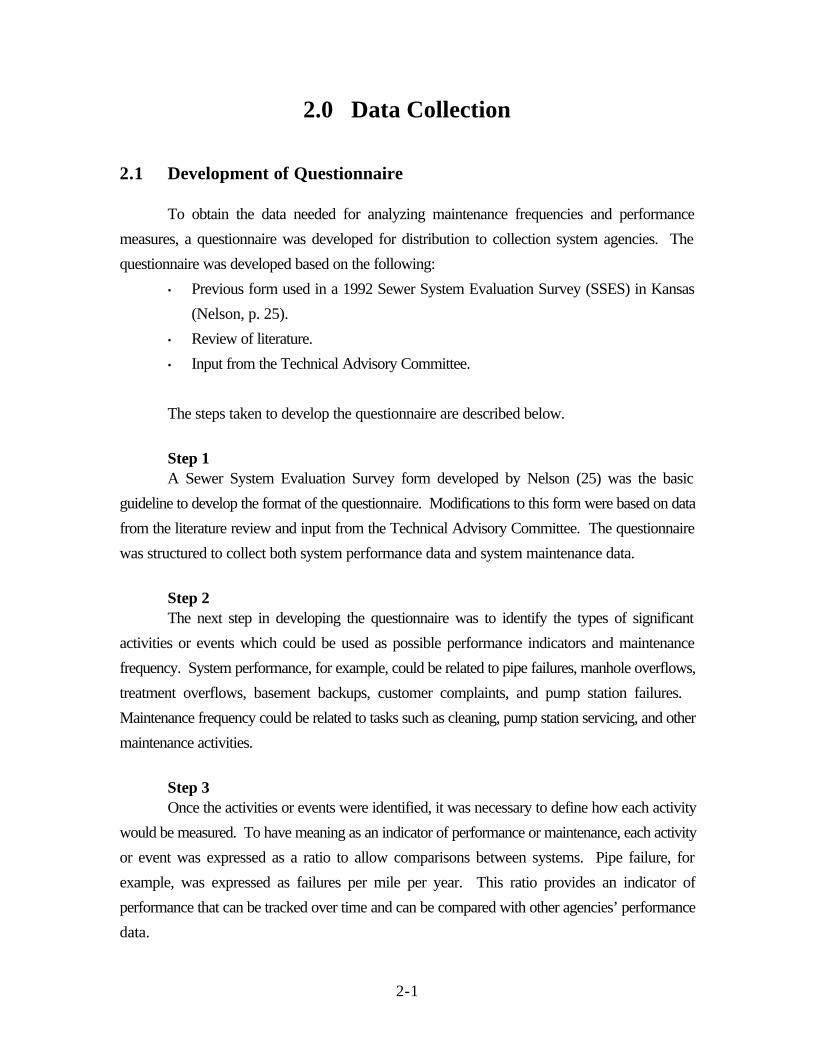
Table 2-1Questionnaire Matrix

Category Data Requested Data NeededService Area Information Miles of Public Sewer

Number of ManholesNumber of ConnectionsArea Served (sq mi)Population ServedAge of System (Age Distribution)

General collection systeminformation.

Flow Information Average Annual Daily FlowMaximum Daily FlowPeak Hourly FlowMaximum Month/Average Daily FlowMinimum Month/Average Daily FlowPercentage of System below theGroundwater Table

General flow informationrepresenting collection system.

System CharacteristicInformation

Percentage of System > 24-inches inDiameterNumber of Pump StationsTotal Installed HorsepowerTotal Energy ConsumedTotal Length of Forcemains, MilesNumber of Equalization BasinsVolume of EqualizationPercentage of System Which isIndustrial/CommercialTypical Velocity of Flow

General characteristic informationrelated to the collection system.

Systems Performance Data Pipe FailuresManhole OverflowsTreatment OverflowsBasement BackupsOthersCustomers ComplaintsPump Station Failures

Cumulative number of events inlast 1 yr, 5 yrs, 10 yrs, and 20 yrs.

Routine MaintenanceFrequencies

Cleaning, Miles of SewerRoot Removal/Treatment, Miles of

Total completed each year from1992 to 1996.

2-3

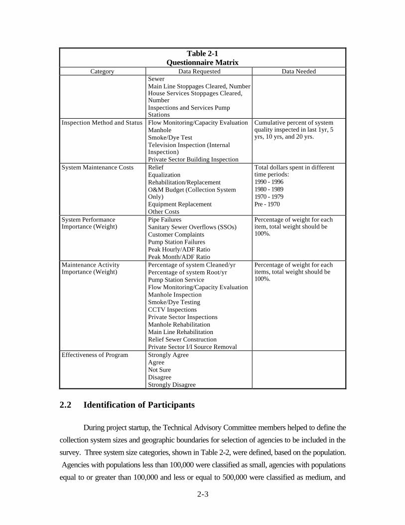
Table 2-1Questionnaire Matrix

Category Data Requested Data NeededSewerMain Line Stoppages Cleared, NumberHouse Services Stoppages Cleared,NumberInspections and Services PumpStations

Inspection Method and Status Flow Monitoring/Capacity EvaluationManholeSmoke/Dye TestTelevision Inspection (InternalInspection)Private Sector Building Inspection

Cumulative percent of systemquality inspected in last 1yr, 5yrs, 10 yrs, and 20 yrs.

System Maintenance Costs ReliefEqualizationRehabilitation/ReplacementO&M Budget (Collection SystemOnly)Equipment ReplacementOther Costs

Total dollars spent in differenttime periods:1990 - 19961980 - 19891970 - 1979Pre - 1970

System PerformanceImportance (Weight)

Pipe FailuresSanitary Sewer Overflows (SSOs)Customer ComplaintsPump Station FailuresPeak Hourly/ADF RatioPeak Month/ADF Ratio

Percentage of weight for eachitem, total weight should be100%.

Maintenance ActivityImportance (Weight)

Percentage of system Cleaned/yrPercentage of system Root/yrPump Station ServiceFlow Monitoring/Capacity EvaluationManhole InspectionSmoke/Dye TestingCCTV InspectionsPrivate Sector InspectionsManhole RehabilitationMain Line RehabilitationRelief Sewer ConstructionPrivate Sector I/I Source Removal

Percentage of weight for eachitems, total weight should be100%.

Effectiveness of Program Strongly AgreeAgreeNot SureDisagreeStrongly Disagree

2.2 Identification of Participants

During project startup, the Technical Advisory Committee members helped to define the

collection system sizes and geographic boundaries for selection of agencies to be included in the

survey. Three system size categories, shown in Table 2-2, were defined, based on the population.

Agencies with populations less than 100,000 were classified as small, agencies with populations

equal to or greater than 100,000 and less or equal to 500,000 were classified as medium, and

2-4

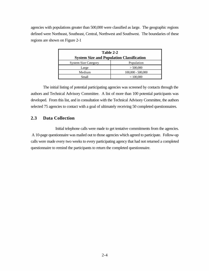
agencies with populations greater than 500,000 were classified as large. The geographic regions

defined were Northeast, Southeast, Central, Northwest and Southwest. The boundaries of these

regions are shown on Figure 2-1

Table 2-2System Size and Population Classification

System Size Category Population

Large > 500,000

Medium 100,000 - 500,000

Small < 100,000

The initial listing of potential participating agencies was screened by contacts through the

authors and Technical Advisory Committee. A list of more than 100 potential participants was

developed. From this list, and in consultation with the Technical Advisory Committee, the authors

selected 75 agencies to contact with a goal of ultimately receiving 50 completed questionnaires.

2.3 Data Collection

Initial telephone calls were made to get tentative commitments from the agencies.

A 10-page questionnaire was mailed out to those agencies which agreed to participate. Follow-up

calls were made every two weeks to every participating agency that had not returned a completed

questionnaire to remind the participants to return the completed questionnaire.

2-5

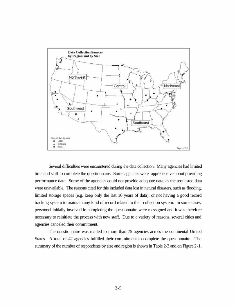
Several difficulties were encountered during the data collection. Many agencies had limited

time and staff to complete the questionnaire. Some agencies were apprehensive about providing

performance data. Some of the agencies could not provide adequate data, as the requested data

were unavailable. The reasons cited for this included data lost in natural disasters, such as flooding,

limited storage spaces (e.g. keep only the last 10 years of data); or not having a good record

tracking system to maintain any kind of record related to their collection system. In some cases,

personnel initially involved in completing the questionnaire were reassigned and it was therefore

necessary to reinitiate the process with new staff. Due to a variety of reasons, several cities and

agencies canceled their commitment.

The questionnaire was mailed to more than 75 agencies across the continental United

States. A total of 42 agencies fulfilled their commitment to complete the questionnaire. The

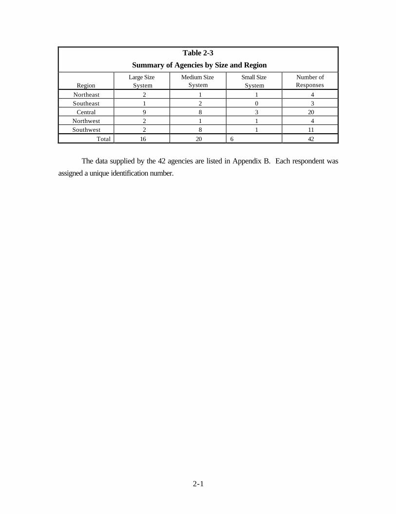
summary of the number of respondents by size and region is shown in Table 2-3 and on Figure 2-1.

2-1

Table 2-3

Summary of Agencies by Size and Region

RegionLarge Size System

Medium SizeSystem

Small SizeSystem

Number ofResponses

Northeast 2 1 1 4

Southeast 1 2 0 3

Central 9 8 3 20

Northwest 2 1 1 4

Southwest 2 8 1 11

Total 16 20 6 42

The data supplied by the 42 agencies are listed in Appendix B. Each respondent was

assigned a unique identification number.

3-1

3.0 Agency Data

3.1 Introduction

All collection systems included in the survey were designed as separate sanitary sewers.

This chapter summarizes the data supplied by the 42 respondents. The majority of the respondents

thought the quality of data in each section was either “very good,” “good,” or “fair.”

3.2 Service Area Characteristics

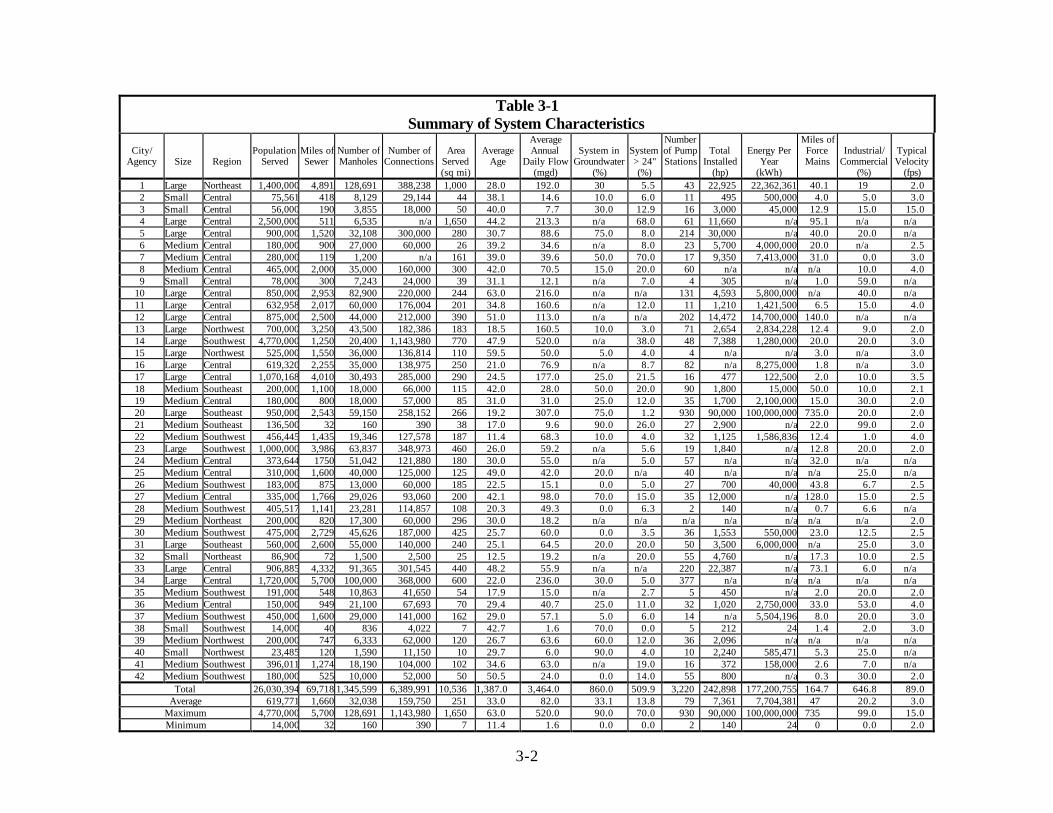
3.2.1 Summary of Service Area InformationEach agency was requested to provide information on, among other things, the total sewer

miles, total number of manholes, total number of connections, service area size, served population,

and the age of the system. The system characteristic data for each agency is presented in Table 3-

1.

The agencies varied widely in terms of size and population served, number of manholes,

and number of connections, with the smallest agency having a service area of 7 square miles and

a population of 14,000, and the largest having a service area of 1,650 square miles and a

population served of 4,770,000. The number of connections ranged from 390 to 1,143,980. The

number of manholes ranged from 160 to 128,691. The miles of sewer ranged from 32 to 5,700.

Some of the data reported indicates a mismatch between people served and miles of sewer. It is

believed that some of these data are for regional systems where the smaller collection sewers

serving the population are not included in the length of sewer reported. In addition, the same data

for several agencies are suspect. As expected, sewer length is proportional to population.

Eliminating these suspect agencies (agencies 4, 5, 7, 14, 21, and 32) results in an average sewer

length density of 1 mile for every 245 people or 21.5 feet of sewer per person. Table 3-2

summarizes the population area, and sewer length by region, size, and average. Figure 3-1 shows

a relationship between miles of sewer and population.

3-2

Table 3-1Summary of System Characteristics

City/Agency Size Region

PopulationServed

Miles ofSewer

Number ofManholes

Number ofConnections

AreaServed(sq mi)

AverageAge

AverageAnnual

Daily Flow(mgd)

System inGroundwater

(%)

System> 24"(%)

Numberof PumpStations

TotalInstalled

(hp)

Energy PerYear

(kWh)

Miles ofForceMains

Industrial/Commercial

(%)

TypicalVelocity

(fps)1 Large Northeast 1,400,000 4,891 128,691 388,238 1,000 28.0 192.0 30 5.5 43 22,925 22,362,361 40.1 19 2.02 Small Central 75,561 418 8,129 29,144 44 38.1 14.6 10.0 6.0 11 495 500,000 4.0 5.0 3.03 Small Central 56,000 190 3,855 18,000 50 40.0 7.7 30.0 12.9 16 3,000 45,000 12.9 15.0 15.04 Large Central 2,500,000 511 6,535 n/a 1,650 44.2 213.3 n/a 68.0 61 11,660 n/a 95.1 n/a n/a5 Large Central 900,000 1,520 32,108 300,000 280 30.7 88.6 75.0 8.0 214 30,000 n/a 40.0 20.0 n/a6 Medium Central 180,000 900 27,000 60,000 26 39.2 34.6 n/a 8.0 23 5,700 4,000,000 20.0 n/a 2.57 Medium Central 280,000 119 1,200 n/a 161 39.0 39.6 50.0 70.0 17 9,350 7,413,000 31.0 0.0 3.08 Medium Central 465,000 2,000 35,000 160,000 300 42.0 70.5 15.0 20.0 60 n/a n/a n/a 10.0 4.09 Small Central 78,000 300 7,243 24,000 39 31.1 12.1 n/a 7.0 4 305 n/a 1.0 59.0 n/a

10 Large Central 850,000 2,953 82,900 220,000 244 63.0 216.0 n/a n/a 131 4,593 5,800,000 n/a 40.0 n/a11 Large Central 632,958 2,017 60,000 176,004 201 34.8 160.6 n/a 12.0 11 1,210 1,421,500 6.5 15.0 4.012 Large Central 875,000 2,500 44,000 212,000 390 51.0 113.0 n/a n/a 202 14,472 14,700,000 140.0 n/a n/a13 Large Northwest 700,000 3,250 43,500 182,386 183 18.5 160.5 10.0 3.0 71 2,654 2,834,228 12.4 9.0 2.014 Large Southwest 4,770,000 1,250 20,400 1,143,980 770 47.9 520.0 n/a 38.0 48 7,388 1,280,000 20.0 20.0 3.015 Large Northwest 525,000 1,550 36,000 136,814 110 59.5 50.0 5.0 4.0 4 n/a n/a 3.0 n/a 3.016 Large Central 619,320 2,255 35,000 138,975 250 21.0 76.9 n/a 8.7 82 n/a 8,275,000 1.8 n/a 3.017 Large Central 1,070,168 4,010 30,493 285,000 290 24.5 177.0 25.0 21.5 16 477 122,500 2.0 10.0 3.518 Medium Southeast 200,000 1,100 18,000 66,000 115 42.0 28.0 50.0 20.0 90 1,800 15,000 50.0 10.0 2.119 Medium Central 180,000 800 18,000 57,000 85 31.0 31.0 25.0 12.0 35 1,700 2,100,000 15.0 30.0 2.020 Large Southeast 950,000 2,543 59,150 258,152 266 19.2 307.0 75.0 1.2 930 90,000 100,000,000 735.0 20.0 2.021 Medium Southeast 136,500 32 160 390 38 17.0 9.6 90.0 26.0 27 2,900 n/a 22.0 99.0 2.022 Medium Southwest 456,445 1,435 19,346 127,578 187 11.4 68.3 10.0 4.0 32 1,125 1,586,836 12.4 1.0 4.023 Large Southwest 1,000,000 3,986 63,837 348,973 460 26.0 59.2 n/a 5.6 19 1,840 n/a 12.8 20.0 2.024 Medium Central 373,644 1750 51,042 121,880 180 30.0 55.0 n/a 5.0 57 n/a n/a 32.0 n/a n/a25 Medium Central 310,000 1,600 40,000 125,000 125 49.0 42.0 20.0 n/a 40 n/a n/a n/a 25.0 n/a26 Medium Southwest 183,000 875 13,000 60,000 185 22.5 15.1 0.0 5.0 27 700 40,000 43.8 6.7 2.527 Medium Central 335,000 1,766 29,026 93,060 200 42.1 98.0 70.0 15.0 35 12,000 n/a 128.0 15.0 2.528 Medium Southwest 405,517 1,141 23,281 114,857 108 20.3 49.3 0.0 6.3 2 140 n/a 0.7 6.6 n/a29 Medium Northeast 200,000 820 17,300 60,000 296 30.0 18.2 n/a n/a n/a n/a n/a n/a n/a 2.030 Medium Southwest 475,000 2,729 45,626 187,000 425 25.7 60.0 0.0 3.5 36 1,553 550,000 23.0 12.5 2.531 Large Southeast 560,000 2,600 55,000 140,000 240 25.1 64.5 20.0 20.0 50 3,500 6,000,000 n/a 25.0 3.032 Small Northeast 86,900 72 1,500 2,500 25 12.5 19.2 n/a 20.0 55 4,760 n/a 17.3 10.0 2.533 Large Central 906,885 4,332 91,365 301,545 440 48.2 55.9 n/a n/a 220 22,387 n/a 73.1 6.0 n/a34 Large Central 1,720,000 5,700 100,000 368,000 600 22.0 236.0 30.0 5.0 377 n/a n/a n/a n/a n/a35 Medium Southwest 191,000 548 10,863 41,650 54 17.9 15.0 n/a 2.7 5 450 n/a 2.0 20.0 2.036 Medium Central 150,000 949 21,100 67,693 70 29.4 40.7 25.0 11.0 32 1,020 2,750,000 33.0 53.0 4.037 Medium Southwest 450,000 1,600 29,000 141,000 162 29.0 57.1 5.0 6.0 14 n/a 5,504,196 8.0 20.0 3.038 Small Southwest 14,000 40 836 4,022 7 42.7 1.6 70.0 0.0 5 212 24 1.4 2.0 3.039 Medium Northwest 200,000 747 6,333 62,000 120 26.7 63.6 60.0 12.0 36 2,096 n/a n/a n/a n/a40 Small Northwest 23,485 120 1,590 11,150 10 29.7 6.0 90.0 4.0 10 2,240 585,471 5.3 25.0 n/a41 Medium Southwest 396,011 1,274 18,190 104,000 102 34.6 63.0 n/a 19.0 16 372 158,000 2.6 7.0 n/a42 Medium Southwest 180,000 525 10,000 52,000 50 50.5 24.0 0.0 14.0 55 800 n/a 0.3 30.0 2.0

Total 26,030,394 69,718 1,345,599 6,389,991 10,536 1,387.0 3,464.0 860.0 509.9 3,220 242,898 177,200,755 164.7 646.8 89.0Average 619,771 1,660 32,038 159,750 251 33.0 82.0 33.1 13.8 79 7,361 7,704,381 47 20.2 3.0

Maximum 4,770,000 5,700 128,691 1,143,980 1,650 63.0 520.0 90.0 70.0 930 90,000 100,000,000 735 99.0 15.0Minimum 14,000 32 160 390 7 11.4 1.6 0.0 0.0 2 140 24 0 0.0 2.0

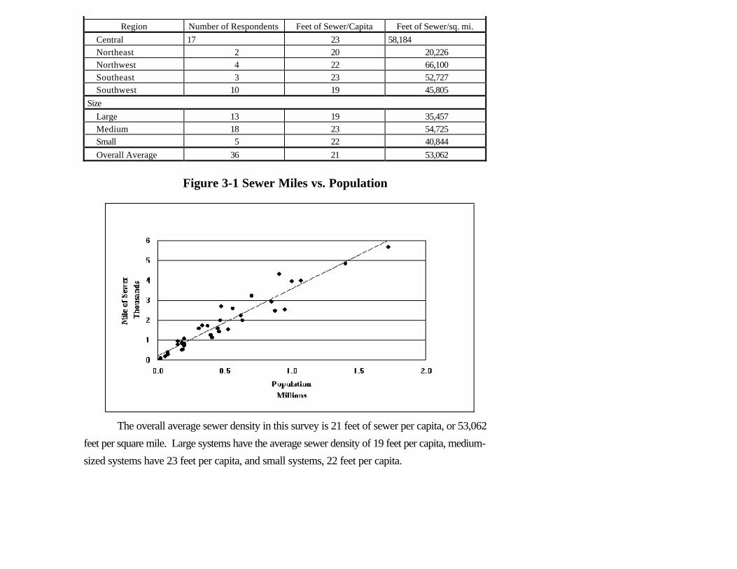
Region Number of Respondents Feet of Sewer/Capita Feet of Sewer/sq. mi.

Central 17 23 58,184

Northeast 2 20 20,226

Northwest 4 22 66,100

Southeast 3 23 52,727

Southwest 10 19 45,805

Size

Large 13 19 35,457

Medium 18 23 54,725

Small 5 22 40,844

Overall Average 36 21 53,062

Figure 3-1 Sewer Miles vs. Population

The overall average sewer density in this survey is 21 feet of sewer per capita, or 53,062

feet per square mile. Large systems have the average sewer density of 19 feet per capita, medium-

sized systems have 23 feet per capita, and small systems, 22 feet per capita.

The age distribution of sewers in a system will vary depending on when development

occurred. Age is an important factor in assessing system needs since systems deteriorate over time.

The oldest collection system in this survey was constructed in 1880. The system age for each

agency was estimated based on the reported percentage of their system within the following age

categories:

• 0 - 10 years (use 5 years as midpoint)



• 51- 100 years (use 75 years as midpoint)

• > 100 years (use 125 years as midpoint)

The average system age ranged from 11.4 to 63 years. The overall average was 33 years.

Average system age for each agency is shown on Figure 3-3

Averaging the cumulative percentages within each class of the age distribution shows that

about 18 percent of sewers were built in the last 10 years, 41 percent in the last 20 years, 82

percent in the last 50 years, and 98 percent in the last 100 years as summarized on Table 3-3 and

shown on Figure 3-4. The average rate of system growth, based upon the age distribution, is

estimated to be about 2.1% per year.

Table 3-3

Percentage of System vs. Average Age

Region

Number ofRespondent

s 0-10 Years(%)

11-20 Years(%)

21-50 Years(%)

51-100 Years(%)

>100 Years(%)

Central 20 13.4 19.7 43.5 21.2 2.2

Northeast 3 21.5 40.4 30.4 7.6 0.0

Northwest 4 19.5 19.0 45.3 12.8 3.5

Southeast 4 27.5 27.3 34.3 10.8 0.3

Southwest 11 21.9 23.4 40.5 13.3 0.9

Size

Large 16 16.3 22.9 39.2 19.5 2.1

Medium 20 20.3 21.5 43.0 13.7 1.5

Small 6 16.0 26.7 39.7 16.8 0.8

Overall 42 18.2 22.8 41.1 16.4 1.6

Cumulative 18.2 40.9 82.0 98.4 100.0

3.3 Flow Information

3.3.1 Summary of Flow Information

Each agency was requested to provide flow information, such as average annual daily flow,

maximum daily flow, peak hourly flow, and maximum and minimum month daily flow.

Average annual daily flows (ADF) reported in the survey ranged from 1.6 to 520 mgd.

The ADF listed in Table 3-4 vary widely, reflecting the differences in the industrial component and

the I/I of flow of each system. Generally, ADF increases with increasing population although the

data shows that ADF cannot be accurately predicted by population estimates alone. The average

per capita ADF is 140 gpcd. Figure 3-5 shows the relationship between ADF and population.

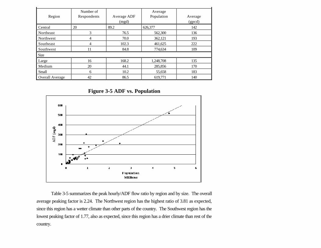
RegionNumber of

Respondents Average ADF(mgd)

AveragePopulation Average

(gpcd)

Central 20 89.2 626,377 142

Northeast 3 76.5 562,300 136

Northwest 4 70.0 362,121 193

Southeast 4 102.3 461,625 222

Southwest 11 84.8 774,634 109

Size

Large 16 168.2 1,248,708 135

Medium 20 44.1 285,856 170

Small 6 10.2 55,658 183

Overall Average 42 86.5 619,771 140

Figure 3-5 ADF vs. Population

Table 3-5 summarizes the peak hourly/ADF flow ratio by region and by size. The overall

average peaking factor is 2.24. The Northwest region has the highest ratio of 3.81 as expected,

since this region has a wetter climate than other parts of the country. The Southwest region has the

lowest peaking factor of 1.77, also as expected, since this region has a drier climate than rest of the

country.

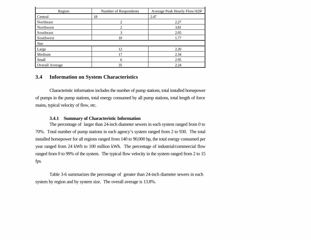
Region Number of Respondents Average Peak Hourly Flow/ADF

Central 18 2.47

Northeast 2 2.27

Northwest 2 3.81

Southeast 3 2.05

Southwest 10 1.77

Size

Large 12 2.20

Medium 17 2.34

Small 6 2.95

Overall Average 35 2.24

3.4 Information on System Characteristics

Characteristic information includes the number of pump stations, total installed horsepower

of pumps in the pump stations, total energy consumed by all pump stations, total length of force

mains, typical velocity of flow, etc.

3.4.1 Summary of Characteristic InformationThe percentage of larger than 24-inch diameter sewers in each system ranged from 0 to

70%. Total number of pump stations in each agency’s system ranged from 2 to 930. The total

installed horsepower for all regions ranged from 140 to 90,000 hp, the total energy consumed per

year ranged from 24 kWh to 100 million kWh. The percentage of industrial/commercial flow

ranged from 0 to 99% of the system. The typical flow velocity in the system ranged from 2 to 15

fps.

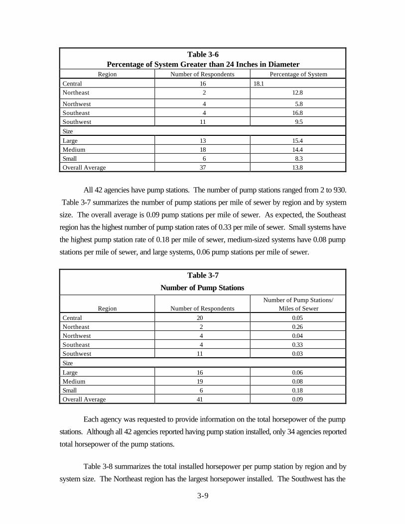
Table 3-6 summarizes the percentage of greater than 24-inch diameter sewers in each

system by region and by system size. The overall average is 13.8%.

3-9

Table 3-6Percentage of System Greater than 24 Inches in Diameter

Region Number of Respondents Percentage of System

Central 16 18.1

Northeast 2 12.8

Northwest 4 5.8

Southeast 4 16.8

Southwest 11 9.5

Size

Large 13 15.4

Medium 18 14.4

Small 6 8.3


All 42 agencies have pump stations. The number of pump stations ranged from 2 to 930.

Table 3-7 summarizes the number of pump stations per mile of sewer by region and by system

size. The overall average is 0.09 pump stations per mile of sewer. As expected, the Southeast

region has the highest number of pump station rates of 0.33 per mile of sewer. Small systems have

the highest pump station rate of 0.18 per mile of sewer, medium-sized systems have 0.08 pump

stations per mile of sewer, and large systems, 0.06 pump stations per mile of sewer.

Table 3-7

Number of Pump Stations

Region Number of RespondentsNumber of Pump Stations/

Miles of Sewer

Central 20 0.05

Northeast 2 0.26

Northwest 4 0.04

Southeast 4 0.33

Southwest 11 0.03

Size

Large 16 0.06

Medium 19 0.08

Small 6 0.18


Each agency was requested to provide information on the total horsepower of the pump

stations. Although all 42 agencies reported having pump station installed, only 34 agencies reported

total horsepower of the pump stations.

Table 3-8 summarizes the total installed horsepower per pump station by region and by

system size. The Northeast region has the largest horsepower installed. The Southwest has the

3-10

smallest horsepower installed. Small systems have larger horsepower installed than large and

medium-seized systems.

Table 3-8

Total Installed Horsepower of Pump Stations

Region Number of Respondents Horsepower/Pump Station

Central 15 110

Northeast 2` 310

Northwest 3 80

Southeast 4 74

Southwest 10 54

Size

Large 13 104

Medium 15 90

Small 6 110

Overall Average 34 98

The average of the total length of force main per pump station is 0.56 miles as summarized

in Table 3-9. The Central region has the highest rates of 0.67 miles of force main per pump station,

and the Northwest region has the lowest rate of 0.36 miles of force main per pump station.

Medium-sized systems have the highest rate of 0.69 miles of force main per pump station, large

systems have 0.45 miles of force main per pump station, and small systems, 0.42 miles of force

main per pump station.

Table 3-9

Ration-Force Main Length/Pump Station

Region Number of Respondents miles/ps

Central 16 0.67

Northeast 2 0.42

Northwest 3 0.36

Southeast 3 0.54

Southwest 11 0.50

Size

Large 13 0.45

Medium 16 0.69

Small 6 0.42


3-11

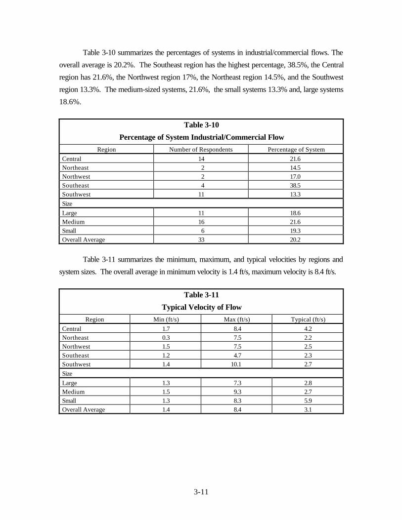
Table 3-10 summarizes the percentages of systems in industrial/commercial flows. The

overall average is 20.2%. The Southeast region has the highest percentage, 38.5%, the Central

region has 21.6%, the Northwest region 17%, the Northeast region 14.5%, and the Southwest

region 13.3%. The medium-sized systems, 21.6%, the small systems 13.3% and, large systems

18.6%.

Table 3-10

Percentage of System Industrial/Commercial Flow

Region Number of Respondents Percentage of System

Central 14 21.6

Northeast 2 14.5

Northwest 2 17.0

Southeast 4 38.5

Southwest 11 13.3

Size

Large 11 18.6

Medium 16 21.6

Small 6 19.3


Table 3-11 summarizes the minimum, maximum, and typical velocities by regions and

system sizes. The overall average in minimum velocity is 1.4 ft/s, maximum velocity is 8.4 ft/s.

Table 3-11

Typical Velocity of Flow

Region Min (ft/s) Max (ft/s) Typical (ft/s)

Central 1.7 8.4 4.2

Northeast 0.3 7.5 2.2

Northwest 1.5 7.5 2.5

Southeast 1.2 4.7 2.3

Southwest 1.4 10.1 2.7

Size

Large 1.3 7.3 2.8

Medium 1.5 9.3 2.7

Small 1.3 8.3 5.9

Overall Average 1.4 8.4 3.1

4-1

4.0 Maintenance Data

4.1 Introduction

Maintenance typically refers to the specific procedures, tasks, instructions, personnel,

qualifications, equipment, and resources needed to satisfy the maintainability requirement within a

specific use environment. AMaintenance is that set of activities required to keep a component,

system, infrastructure asset, or facility functioning as it was originally designed and constructed to

function.@1 For our purpose, any reinvestment in the system, including routine maintenance, capital

improvements for repair or rehabilitation, inspection activities, and monitoring activities are classified

as maintenance. Capital improvements for system expansion are not classified as maintenance

reinvestment.

4.2 Routine Maintenance

Routine maintenance includes sewer cleaning, root removal/treatment, cleaning of mainline

stoppages, cleaning of house service stoppages, and inspections and servicing of pump stations.

Each agency was requested to provide 5 years of data (from 1992 to 1996) to establish routine

maintenance rates. These routine maintenance rates by region and by size are presented in Table

4-1 through 4-5.

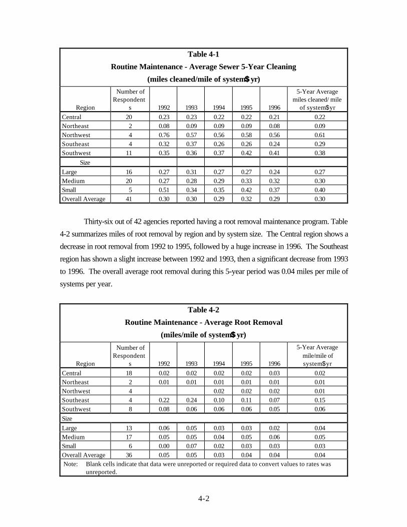
Forty-one out of 42 agencies reported having a cleaning maintenance program. Table 4-1

summarizes the sewer maintenance for each year from 1992 to 1996 by region and system size.

The cleaning rates represented the reported total miles cleaned annually compared to the total miles

in the agency=s system. Overall, the Northwest region has the highest cleaning rates in miles per

mile per year, and the Northeast has the lowest rate in miles per mile per year. Small systems have

the highest cleaning rate, followed by medium and large systems. Overall, the annual cleaning rate

varied from about 0.29 miles per mile per year to about 0.32 miles per mile per year. The overall

average cleaning rate is 0.30 miles per mile per year.

1Ronald Hudson, Infrastructure Management.

4-2

Table 4-1

Routine Maintenance - Average Sewer 5-Year Cleaning

(miles cleaned/mile of system$$yr)

Region

Number ofRespondent

s 1992 1993 1994 1995 1996

5-Year Averagemiles cleaned/ mile

of system$yr

Central 20 0.23 0.23 0.22 0.22 0.21 0.22

Northeast 2 0.08 0.09 0.09 0.09 0.08 0.09

Northwest 4 0.76 0.57 0.56 0.58 0.56 0.61

Southeast 4 0.32 0.37 0.26 0.26 0.24 0.29

Southwest 11 0.35 0.36 0.37 0.42 0.41 0.38

Size

Large 16 0.27 0.31 0.27 0.27 0.24 0.27

Medium 20 0.27 0.28 0.29 0.33 0.32 0.30

Small 5 0.51 0.34 0.35 0.42 0.37 0.40

Overall Average 41 0.30 0.30 0.29 0.32 0.29 0.30

Thirty-six out of 42 agencies reported having a root removal maintenance program. Table

4-2 summarizes miles of root removal by region and by system size. The Central region shows a

decrease in root removal from 1992 to 1995, followed by a huge increase in 1996. The Southeast

region has shown a slight increase between 1992 and 1993, then a significant decrease from 1993

to 1996. The overall average root removal during this 5-year period was 0.04 miles per mile of

systems per year.

Table 4-2

Routine Maintenance - Average Root Removal

(miles/mile of system$$yr)

Region

Number ofRespondent

s 1992 1993 1994 1995 1996

5-Year Averagemile/mile ofsystem$yr

Central 18 0.02 0.02 0.02 0.02 0.03 0.02

Northeast 2 0.01 0.01 0.01 0.01 0.01 0.01

Northwest 4 0.02 0.02 0.02 0.01

Southeast 4 0.22 0.24 0.10 0.11 0.07 0.15

Southwest 8 0.08 0.06 0.06 0.06 0.05 0.06

Size

Large 13 0.06 0.05 0.03 0.03 0.02 0.04

Medium 17 0.05 0.05 0.04 0.05 0.06 0.05

Small 6 0.00 0.07 0.02 0.03 0.03 0.03

Overall Average 36 0.05 0.05 0.03 0.04 0.04 0.04

Note: Blank cells indicate that data were unreported or required data to convert values to rates wasunreported.

4-3

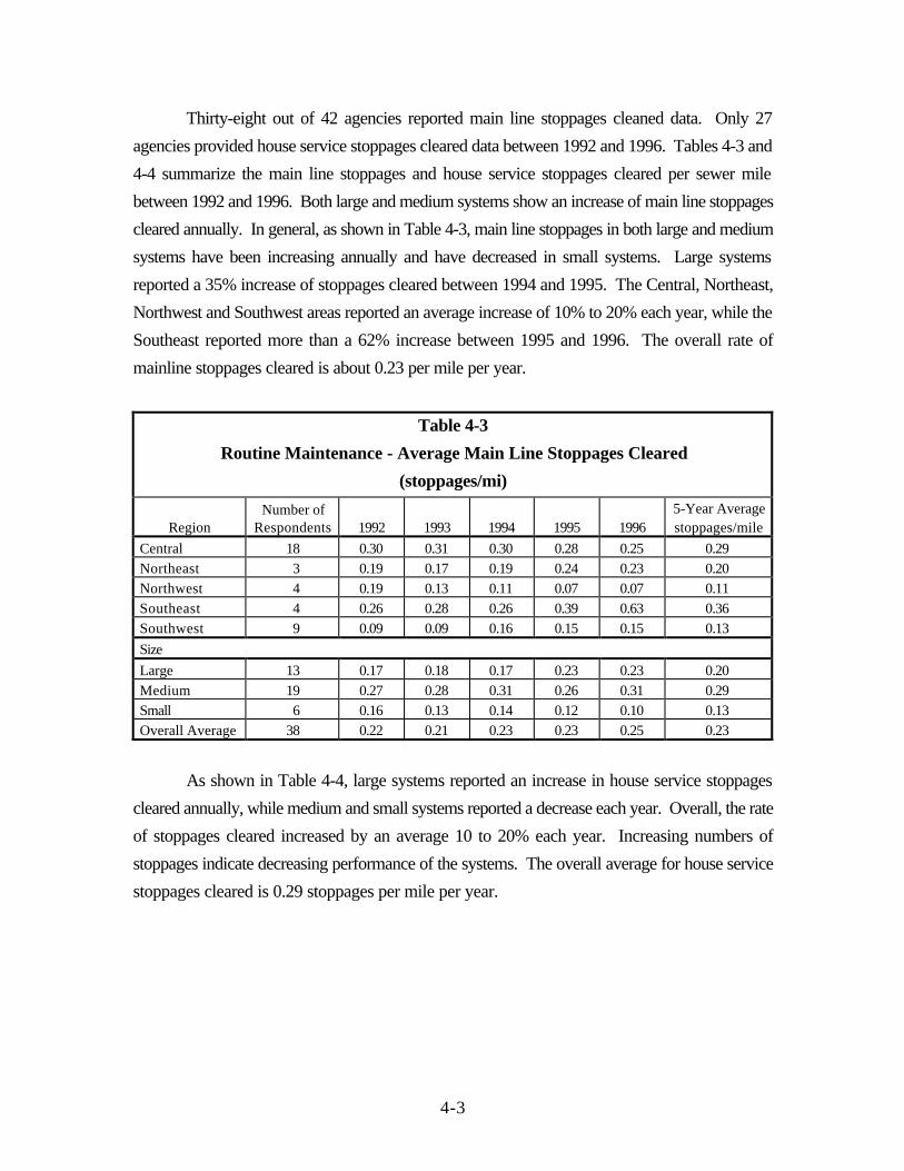
Thirty-eight out of 42 agencies reported main line stoppages cleaned data. Only 27

agencies provided house service stoppages cleared data between 1992 and 1996. Tables 4-3 and

4-4 summarize the main line stoppages and house service stoppages cleared per sewer mile

between 1992 and 1996. Both large and medium systems show an increase of main line stoppages

cleared annually. In general, as shown in Table 4-3, main line stoppages in both large and medium

systems have been increasing annually and have decreased in small systems. Large systems

reported a 35% increase of stoppages cleared between 1994 and 1995. The Central, Northeast,

Northwest and Southwest areas reported an average increase of 10% to 20% each year, while the

Southeast reported more than a 62% increase between 1995 and 1996. The overall rate of

mainline stoppages cleared is about 0.23 per mile per year.

Table 4-3

Routine Maintenance - Average Main Line Stoppages Cleared

(stoppages/mi)

RegionNumber of

Respondents 1992 1993 1994 1995 19965-Year Averagestoppages/mile

Central 18 0.30 0.31 0.30 0.28 0.25 0.29

Northeast 3 0.19 0.17 0.19 0.24 0.23 0.20

Northwest 4 0.19 0.13 0.11 0.07 0.07 0.11

Southeast 4 0.26 0.28 0.26 0.39 0.63 0.36

Southwest 9 0.09 0.09 0.16 0.15 0.15 0.13

Size

Large 13 0.17 0.18 0.17 0.23 0.23 0.20

Medium 19 0.27 0.28 0.31 0.26 0.31 0.29

Small 6 0.16 0.13 0.14 0.12 0.10 0.13

Overall Average 38 0.22 0.21 0.23 0.23 0.25 0.23

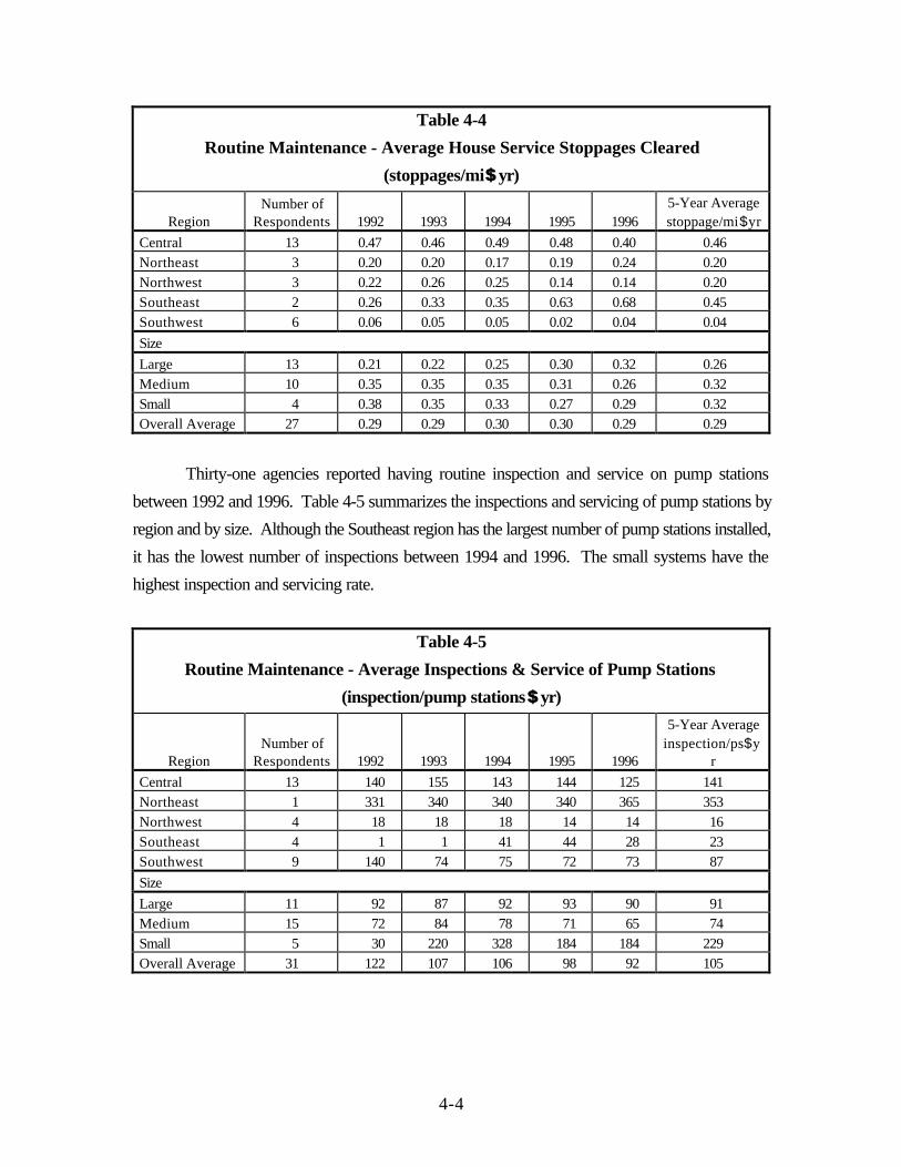
As shown in Table 4-4, large systems reported an increase in house service stoppages

cleared annually, while medium and small systems reported a decrease each year. Overall, the rate

of stoppages cleared increased by an average 10 to 20% each year. Increasing numbers of

stoppages indicate decreasing performance of the systems. The overall average for house service

stoppages cleared is 0.29 stoppages per mile per year.

4-4

Table 4-4

Routine Maintenance - Average House Service Stoppages Cleared

(stoppages/mi$$yr)

RegionNumber of

Respondents 1992 1993 1994 1995 19965-Year Averagestoppage/mi$yr

Central 13 0.47 0.46 0.49 0.48 0.40 0.46

Northeast 3 0.20 0.20 0.17 0.19 0.24 0.20

Northwest 3 0.22 0.26 0.25 0.14 0.14 0.20

Southeast 2 0.26 0.33 0.35 0.63 0.68 0.45

Southwest 6 0.06 0.05 0.05 0.02 0.04 0.04

Size

Large 13 0.21 0.22 0.25 0.30 0.32 0.26

Medium 10 0.35 0.35 0.35 0.31 0.26 0.32

Small 4 0.38 0.35 0.33 0.27 0.29 0.32

Overall Average 27 0.29 0.29 0.30 0.30 0.29 0.29

Thirty-one agencies reported having routine inspection and service on pump stations

between 1992 and 1996. Table 4-5 summarizes the inspections and servicing of pump stations by

region and by size. Although the Southeast region has the largest number of pump stations installed,

it has the lowest number of inspections between 1994 and 1996. The small systems have the

highest inspection and servicing rate.

Table 4-5

Routine Maintenance - Average Inspections & Service of Pump Stations

(inspection/pump stations$$yr)

RegionNumber of

Respondents 1992 1993 1994 1995 1996

5-Year Averageinspection/ps$y

r

Central 13 140 155 143 144 125 141

Northeast 1 331 340 340 340 365 353

Northwest 4 18 18 18 14 14 16

Southeast 4 1 1 41 44 28 23

Southwest 9 140 74 75 72 73 87

Size

Large 11 92 87 92 93 90 91

Medium 15 72 84 78 71 65 74

Small 5 30 220 328 184 184 229

Overall Average 31 122 107 106 98 92 105

4-5

4.3 Inspection Maintenance

An inspection program is vital to proper maintenance of a wastewater collection system.

Without inspections, a maintenance program is difficult to define, since problems cannot be solved

if they are not identified. The elements of an inspection program include flow monitoring, manhole

inspections, smoke/dye testing, closed circuit television inspection, and private sector inspections.

Inspections provide the data necessary for managers to make informed decisions on all

maintenance, repair, and rehabilitation actions.

Information regarding the inspection methods and status for the most recent 1-year, 5-year,

10-year, and 20-year time intervals was obtained for each agency. Cumulative numbers of

inspections completed for each type of activity were obtained. The inspection maintenance

methods by region and by size are summarized in Tables 4-6 through 4-10.

The frequency and types of inspections vary widely from agency to agency.

Table 4-6 summarizes the flow evaluations performed by region and by size in the last 1

year, 5 years, 10 years, and 20 years. The Northwest and Southwest regions reported greater

flow monitoring activities than the other regions. Large systems reported more flow monitoring than

medium or small systems. Overall, flow monitoring has increased from 8% per year 20 years ago

to 33% per year today. Some areas have been monitored more than once and therefore, have

been reported as being flow monitored more than once resulting in reported values exceeding

100%.

Table 4-6Inspection Methods - Flow Evaluation

(cumulative % of system)

RegionNumber of

Respondents 1-Year 5-Year 10-Year 20-YearCentral 15 26% 53% 74% 83%Northeast 3 63% 67% 67% 67%Northwest 3 67% 367% 533% 733%Southeast 4 15% 43% 43% 43%Southwest 8 32% 67% 106% 170%SizeLarge 10 53% 143% 220% 331%Medium 17 33% 68% 76% 77%Small 6 2% 35% 74% 91%Overall Average 33 33% 85% 119% 157%Average %/Year 33% 17% 12% 8%

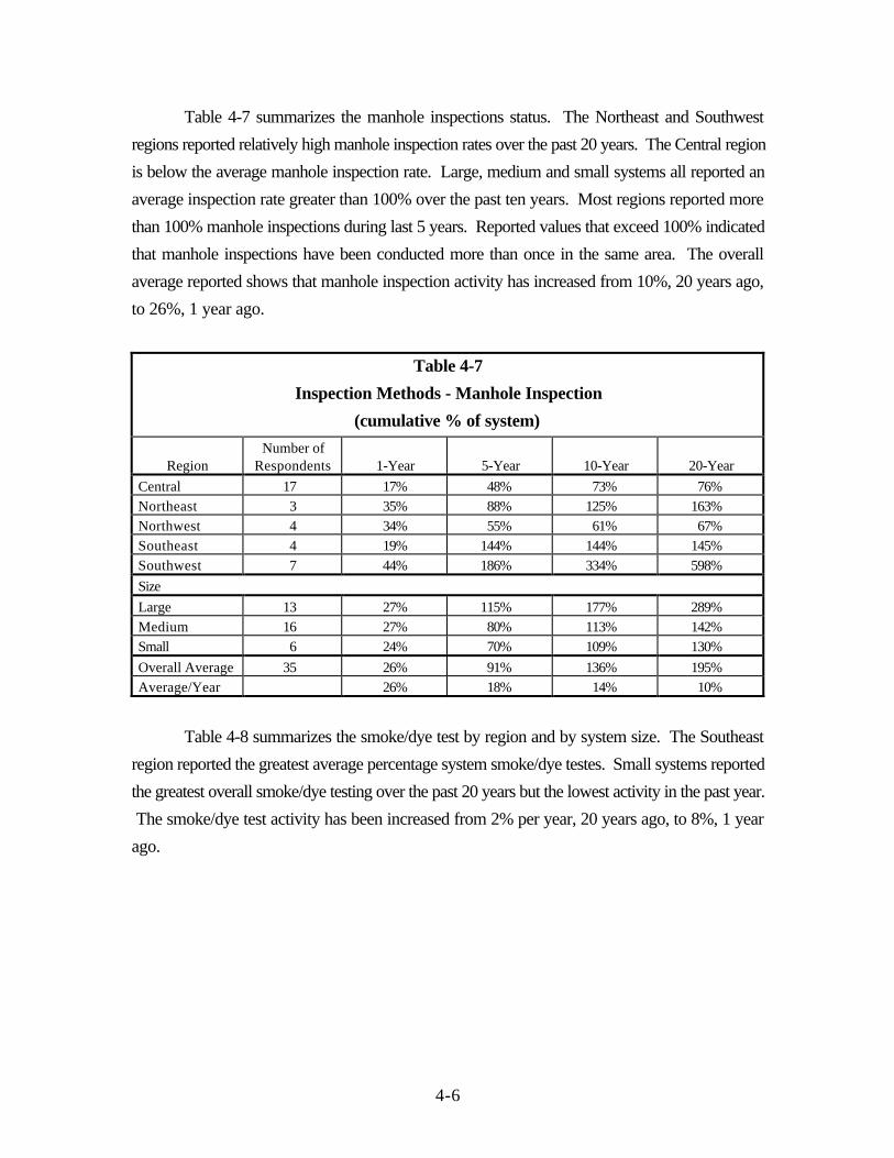
4-6

Table 4-7 summarizes the manhole inspections status. The Northeast and Southwest

regions reported relatively high manhole inspection rates over the past 20 years. The Central region

is below the average manhole inspection rate. Large, medium and small systems all reported an

average inspection rate greater than 100% over the past ten years. Most regions reported more

than 100% manhole inspections during last 5 years. Reported values that exceed 100% indicated

that manhole inspections have been conducted more than once in the same area. The overall

average reported shows that manhole inspection activity has increased from 10%, 20 years ago,

to 26%, 1 year ago.

Table 4-7

Inspection Methods - Manhole Inspection


RegionNumber of

Respondents 1-Year 5-Year 10-Year 20-Year

Central 17 17% 48% 73% 76%

Northeast 3 35% 88% 125% 163%

Northwest 4 34% 55% 61% 67%

Southeast 4 19% 144% 144% 145%

Southwest 7 44% 186% 334% 598%

Size

Large 13 27% 115% 177% 289%

Medium 16 27% 80% 113% 142%

Small 6 24% 70% 109% 130%

Overall Average 35 26% 91% 136% 195%

Average/Year 26% 18% 14% 10%

Table 4-8 summarizes the smoke/dye test by region and by system size. The Southeast

region reported the greatest average percentage system smoke/dye testes. Small systems reported

the greatest overall smoke/dye testing over the past 20 years but the lowest activity in the past year.

The smoke/dye test activity has been increased from 2% per year, 20 years ago, to 8%, 1 year

ago.

4-7

Table 4-8

Inspection Methods - Smoke/Dye Testing


RegionNumber of


Central 18 12% 21% 31% 38%

Northeast 3 1% 3% 3% 5%

Northwest 4 2% 8% 15% 21%

Southeast 4 13% 123% 123% 123%

Southwest 9 1% 17% 23% 34%

Size

Large 14 10% 33% 35% 37%

Medium 18 7% 20% 27% 33%

Small 6 33% 42% 60%

Overall Average 38 8% 26% 32% 39%

Average/Year 8% 5% 3% 2%


Table 4-9 summarizes TV inspection activity. Overall, TV inspection has increased from

2% per year 20 years ago to 7% per year a year ago. The Southeast region has shown the highest

percentage of TV inspection within the past 5 years.

Table 4-9

Inspection Methods - Television Inspection


RegionNumber of


Central 19 6% 19% 29% 32%

Northeast 3 8% 15% 17% 24%

Northwest 4 7% 36% 45% 55%

Southeast 4 9% 105% 107% 111%

Southwest 9 10% 27% 35% 43%

Size

Large 15 7% 41% 47% 54%

Medium 18 6% 25% 30% 34%

Small 6 11% 25% 48% 54%


Average %/Year 7% 6% 4% 2%

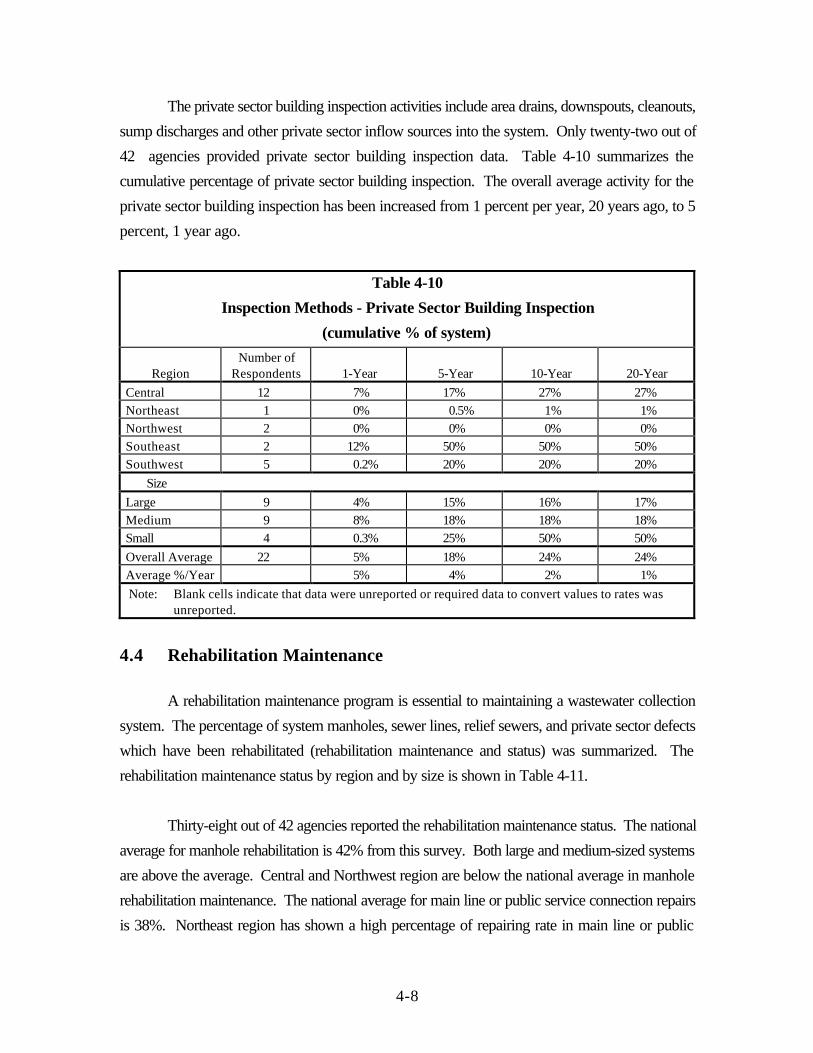
4-8

The private sector building inspection activities include area drains, downspouts, cleanouts,

sump discharges and other private sector inflow sources into the system. Only twenty-two out of

42 agencies provided private sector building inspection data. Table 4-10 summarizes the

cumulative percentage of private sector building inspection. The overall average activity for the

private sector building inspection has been increased from 1 percent per year, 20 years ago, to 5

percent, 1 year ago.

Table 4-10

Inspection Methods - Private Sector Building Inspection


RegionNumber of


Central 12 7% 17% 27% 27%

Northeast 1 0% 0.5% 1% 1%

Northwest 2 0% 0% 0% 0%

Southeast 2 12% 50% 50% 50%

Southwest 5 0.2% 20% 20% 20%

Size

Large 9 4% 15% 16% 17%

Medium 9 8% 18% 18% 18%

Small 4 0.3% 25% 50% 50%


Average %/Year 5% 4% 2% 1%


4.4 Rehabilitation Maintenance

A rehabilitation maintenance program is essential to maintaining a wastewater collection

system. The percentage of system manholes, sewer lines, relief sewers, and private sector defects

which have been rehabilitated (rehabilitation maintenance and status) was summarized. The

rehabilitation maintenance status by region and by size is shown in Table 4-11.

Thirty-eight out of 42 agencies reported the rehabilitation maintenance status. The national

average for manhole rehabilitation is 42% from this survey. Both large and medium-sized systems

are above the average. Central and Northwest region are below the national average in manhole

rehabilitation maintenance. The national average for main line or public service connection repairs

is 38%. Northeast region has shown a high percentage of repairing rate in main line or public

4-9

service connection. The national average relief sewer rehabilitation maintenance is 47%. The small

systems have the highest maintenance rate of 81%. The national average for private sector

maintenance is 28%. Southwest region and small systems have the highest maintenance rate.

Table 4-11

Rehabilitation Maintenance Status

RegionNumber of

Respondents Manhole

Main Line or PublicService Connection

Repairs Relief/Equalization Private Sector

Central 18 35% 33% 42% 21%

Northeast 2 83% 73% 80% 0 %

Northwest 4 35% 28% 50% 34%

Southeast 4 51% 41% 32% 32%

Southwest 10 45% 40% 55% 49%

Size

Large 14 46% 36% 44% 26%

Medium 18 43% 39% 44% 26%

Small 6 32% 39% 81% 44%



4.5 System Maintenance Costs

System maintenance costs were reported by the following categories: relief, equalization,

rehabilitation/replacement, routine O&M, equipment replacement, and other costs. Information

regarding the total dollars reinvested on system maintenance was obtained for the following time

periods:

$ 1990 - 1996

$ 1980 - 1989

$ 1970 - 1979

$ pre - 1970

The dollar values listed are as reported and are not adjusted for inflation.

The average cumulative dollars spent on system maintenance is listed in Tables 4-12

through 4-15. The data show a large increase in spending in the 1990s. The rate of spending has

increased from $5 per mile per year in pre-1970s to $8,000 per mile per year in the 1990s as

indicated in Table 4-16.

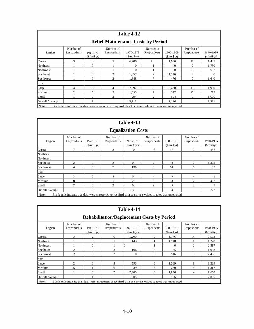
4-10

Table 4-12

Relief Maintenance Costs by Period

RegionNumber of

Respondents Pre-1970($/mi$yr)

Number ofRespondents 1970-1979

($/mi$yr)


($/mi$yr)


($/mi$yr)

Central 3 3 5 6,206 9 1,906 17 1,467

Northeast 1 0 1 0 1 0 2 1,730

Northwest 1 0 1 0 1 0 3 907

Southeast 1 0 2 1,057 2 1,216 4 0

Southwest 1 0 2 1,648 7 476 7 1,640

Size

Large 4 0 4 7,597 6 2,480 13 1,980

Medium 2 5 5 1,093 12 577 15 572

Small 1 0 2 294 2 554 5 1,656

Overall Average 1 3,313 1,146 1,291

Note: Blank cells indicate that data were unreported or required data to convert values to rates was unreported.

Table 4-13

Equalization Costs

RegionNumber of

Respondents Pre-1970($/mi�yr)


($/mi$yr)


($/mi$yr)


($/mi$yr)

Central 7 0 8 0 8 17 10 257

Northeast

Northwest

Southeast 2 0 2 0 2 0 2 1,325

Southwest 4 0 7 130 6 68 6 97

Size

Large 3 0 4 0 4 0 4 1

Medium 8 0 11 82 10 53 12 482

Small 2 0 2 0 2 6 2 7

Overall Average 0 53 34 322


Table 4-14

Rehabilitation/Replacement Costs by Period

RegionNumber of



($/mi$yr)


($/mi$yr)


($/mi$yr)

Central 3 2 6 1,209 9 1,176 14 3,583

Northeast 1 3 1 143 1 1,718 1 1,270

Northwest 1 0 1 0 1 0 2 2,517

Southeast 2 0 3 106 3 65 3 1,098

Southwest 2 0 2 0 8 516 8 2,456

Size

Large 2 0 5 593 6 1,269 9 3,229

Medium 5 1 6 39 13 260 15 1,317

Small 1 0 2 2,205 3 1,876 4 7,650

Overall Average 1 585 756 2,836


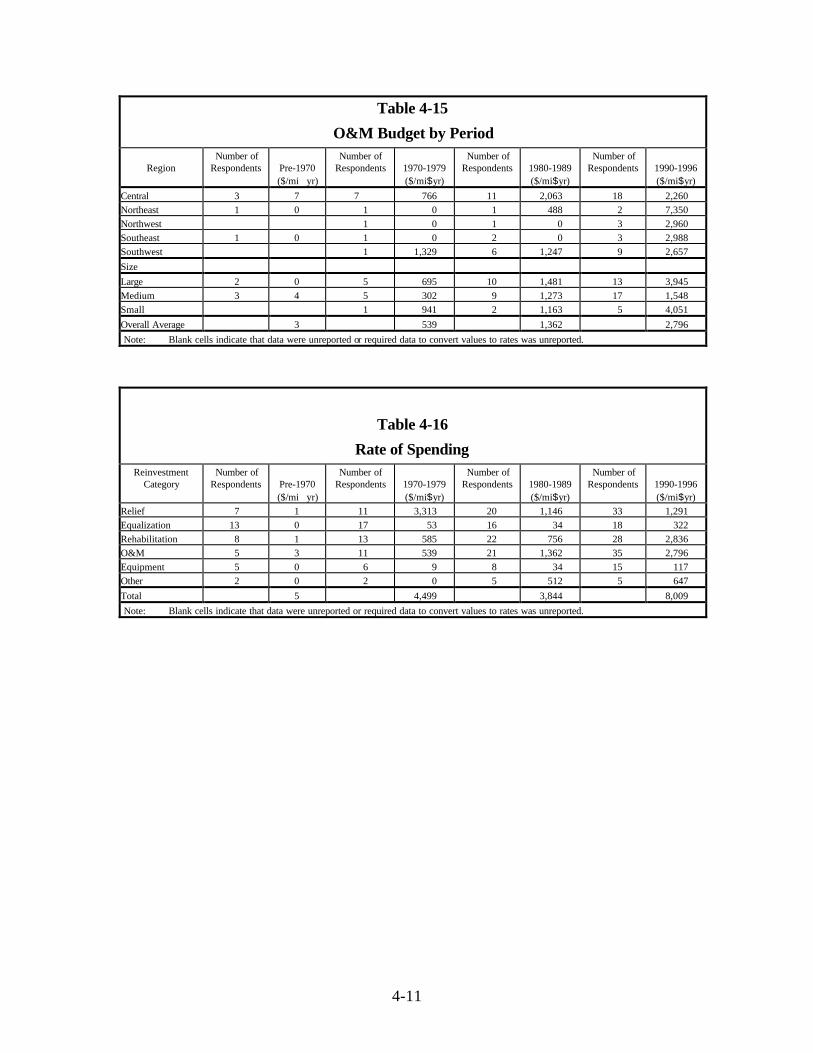
4-11

Table 4-15

O&M Budget by Period

RegionNumber of



($/mi$yr)


($/mi$yr)


($/mi$yr)

Central 3 7 7 766 11 2,063 18 2,260

Northeast 1 0 1 0 1 488 2 7,350

Northwest 1 0 1 0 3 2,960

Southeast 1 0 1 0 2 0 3 2,988

Southwest 1 1,329 6 1,247 9 2,657

Size

Large 2 0 5 695 10 1,481 13 3,945

Medium 3 4 5 302 9 1,273 17 1,548

Small 1 941 2 1,163 5 4,051

Overall Average 3 539 1,362 2,796


Table 4-16

Rate of SpendingReinvestment

CategoryNumber of



($/mi$yr)


($/mi$yr)


($/mi$yr)

Relief 7 1 11 3,313 20 1,146 33 1,291

Equalization 13 0 17 53 16 34 18 322

Rehabilitation 8 1 13 585 22 756 28 2,836

O&M 5 3 11 539 21 1,362 35 2,796

Equipment 5 0 6 9 8 34 15 117

Other 2 0 2 0 5 512 5 647

Total 5 4,499 3,844 8,009


5-1

5.0 System Maintenance Frequency Determination

5.1 Introduction

Maintenance, as defined in the broad sense used in this study, includes any collection

system reinvestment in the form of capital improvements, rehabilitation, inspection, and what is

typically considered routine maintenance. All maintenance activities are not equally effective.

Therefore, when evaluating how much maintenance an agency is doing, what is of real interest is

how much effective maintenance it is doing. For example, if an agency was performing only

CCTV inspections and nothing else, even though considerable time and effort may be going into

the CCTV inspection, little system improvement would result. The CCTV is effective only if it is

done in concert with other activities such as removing blockages and debris or repairing defects.

In other words, an effective maintenance program requires a balance of activities. This chapter

presents an evaluation of maintenance and a determination of a maintenance frequency for the

agencies surveyed.

5.2 Weighting of Maintenance Activities

In order to evaluate the relative importance of activities necessary to develop a system

maintenance frequency, each agency was requested to provide an opinion of the relative importance

of twelve common maintenance activities. The most important maintenance activity, as selected by

the agencies surveyed, is line cleaning, which averaged almost 18% of the total maintenance weight

assigned. The next three activities, listed in descending order of importance, are pump station

servicing (14.1%), main line rehabilitation (12.6%), and closed circuit television inspection (10.5%).

The three least important activities, as selected by the agencies surveyed, are manhole rehabilitation

(5.6%), smoke testing (3.3%), and private sector inspections (2.0%). These maintenance activities

and their average weight of importance are listed in Table 5-1. Average percentages were adjusted

proportionately, so that the total of all maintenance items was equal to 100 percent.

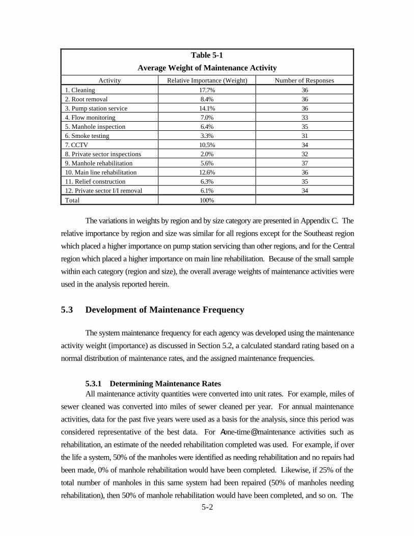
5-2

Table 5-1

Average Weight of Maintenance Activity

Activity Relative Importance (Weight) Number of Responses

1. Cleaning 17.7% 36

2. Root removal 8.4% 36

3. Pump station service 14.1% 36

4. Flow monitoring 7.0% 33

5. Manhole inspection 6.4% 35

6. Smoke testing 3.3% 31

7. CCTV 10.5% 34

8. Private sector inspections 2.0% 32

9. Manhole rehabilitation 5.6% 37

10. Main line rehabilitation 12.6% 36

11. Relief construction 6.3% 35

12. Private sector I/I removal 6.1% 34

Total 100%

The variations in weights by region and by size category are presented in Appendix C. The

relative importance by region and size was similar for all regions except for the Southeast region

which placed a higher importance on pump station servicing than other regions, and for the Central

region which placed a higher importance on main line rehabilitation. Because of the small sample

within each category (region and size), the overall average weights of maintenance activities were

used in the analysis reported herein.

5.3 Development of Maintenance Frequency

The system maintenance frequency for each agency was developed using the maintenance

activity weight (importance) as discussed in Section 5.2, a calculated standard rating based on a

normal distribution of maintenance rates, and the assigned maintenance frequencies.

5.3.1 Determining Maintenance RatesAll maintenance activity quantities were converted into unit rates. For example, miles of

sewer cleaned was converted into miles of sewer cleaned per year. For annual maintenance

activities, data for the past five years were used as a basis for the analysis, since this period was

considered representative of the best data. For Aone-time@ maintenance activities such as

rehabilitation, an estimate of the needed rehabilitation completed was used. For example, if over

the life a system, 50% of the manholes were identified as needing rehabilitation and no repairs had

been made, 0% of manhole rehabilitation would have been completed. Likewise, if 25% of the

total number of manholes in this same system had been repaired (50% of manholes needing

rehabilitation), then 50% of manhole rehabilitation would have been completed, and so on. The

5-3

time interval during which rehabilitation was done was assumed to be the most recent 25 years,

which approximates the life expectancy of many rehabilitation methods. The maintenance done by

the agencies surveyed is presented in Table 5-2 and the maintenance rates are given in Table 5-3.

To determine maintenance rates, the average miles of sewer installed were estimated over the

maintenance period, based on the age information provided by each agency.

5.3.2 Developing the Standard RatingA standardized table was developed using the maintenance data collected and a normal

distribution. The mean, standard deviation, range, and number of responses for each maintenance

activity are listed in Table 5-4. The rate of each maintenance activity was normalized using the

normal distribution to develop a standard by which any maintenance rate, or group of maintenance

rates from various maintenance activities, could be compared. The frequency of individual

maintenance activities can be easily determined; however, the overall system maintenance

frequency, considering all maintenance activities, requires a method to standardize and weight all

maintenance activities. Once the maintenance data was normalized, a frequency was assigned to

correspond to selected standard deviations from the mean. The assignment of the standard

maintenance frequency was somewhat arbitrary; however, based on previous reports (Nelson) a

5 to 10 percent overall average frequency goal was assumed to be reasonable. Through trial and

error, an average maintenance frequency of 6.7% for all agencies was chosen. This is discussed

in more detail in Section 5.4. The selected frequencies corresponding to the normalized data are

listed in Table 5-5.

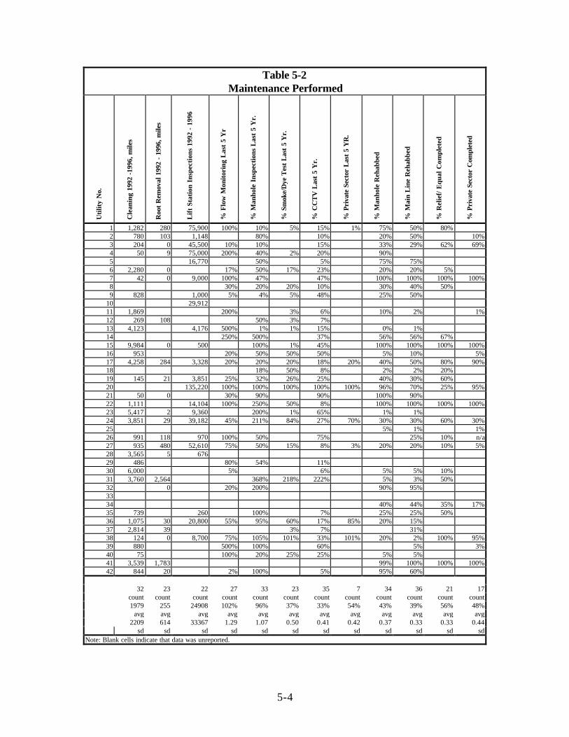
5-4

Table 5-2Maintenance Performed

Uti

lity

No.

Cle

anin

g 19

92 -

1996

, mile

s

Roo

t R

emov

al 1

992

- 19

96, m

iles

Lif

t St

atio

n In

spec

tion

s 19

92 -

199

6

% F

low

Mon

itor

ing

Las

t 5

Yr

% M

anho

le I

nspe

ctio

ns L

ast

5 Y

r.

% S

mok

e/D

ye T

est

Las

t 5

Yr.

% C

CT

V L

ast

5 Y

r.

% P

riva

te S

ecto

r L

ast

5 Y

R.

% M

anho

le R

ehab

bed

% M

ain

Lin

e R

ehab

bed

% R

elie

f/ E

qual

Com

plet

ed

% P

riva

te S

ecto

r C

ompl

eted

1 1,282 280 75,900 100% 10% 5% 15% 1% 75% 50% 80%2 780 103 1,148 80% 10% 20% 50% 10%3 204 0 45,500 10% 10% 15% 33% 29% 62% 69%4 50 9 75,000 200% 40% 2% 20% 90%5 16,770 50% 5% 75% 75%6 2,280 0 17% 50% 17% 23% 20% 20% 5%7 42 0 9,000 100% 47% 47% 100% 100% 100% 100%8 30% 20% 20% 10% 30% 40% 50%9 828 1,000 5% 4% 5% 48% 25% 50%

10 29,91211 1,869 200% 3% 6% 10% 2% 1%12 269 108 50% 3% 7%13 4,123 4,176 500% 1% 1% 15% 0% 1%14 250% 500% 37% 56% 56% 67%15 9,984 0 500 100% 1% 45% 100% 100% 100% 100%16 953 20% 50% 50% 50% 5% 10% 5%17 4,258 284 3,328 20% 20% 20% 18% 20% 40% 50% 80% 90%18 18% 50% 8% 2% 2% 20%19 145 21 3,851 25% 32% 26% 25% 40% 30% 60%20 135,220 100% 100% 100% 100% 100% 96% 70% 25% 95%21 50 0 30% 90% 90% 100% 90%22 1,111 14,104 100% 250% 50% 8% 100% 100% 100% 100%23 5,417 2 9,360 200% 1% 65% 1% 1%24 3,851 29 39,182 45% 211% 84% 27% 70% 30% 30% 60% 30%25 5% 1% 1%26 991 118 970 100% 50% 75% 25% 10% n/a27 935 480 52,610 75% 50% 15% 8% 3% 20% 20% 10% 5%28 3,565 5 67629 486 80% 54% 11%30 6,000 5% 6% 5% 5% 10%31 3,760 2,564 368% 218% 222% 5% 3% 50%32 0 20% 200% 90% 95%3334 40% 44% 35% 17%35 739 260 100% 7% 25% 25% 50%36 1,075 30 20,800 55% 95% 60% 17% 85% 20% 15%37 2,814 39 3% 7% 31%38 124 0 8,700 75% 105% 101% 33% 101% 20% 2% 100% 95%39 880 500% 100% 60% 5% 3%40 75 100% 20% 25% 25% 5% 5%41 3,539 1,783 99% 100% 100% 100%42 844 20 2% 100% 5% 95% 60%

32 23 22 27 33 23 35 7 34 36 21 17count count count count count count count count count count count count1979 255 24908 102% 96% 37% 33% 54% 43% 39% 56% 48%

avg avg avg avg avg avg avg avg avg avg avg avg2209 614 33367 1.29 1.07 0.50 0.41 0.42 0.37 0.33 0.33 0.44

sd sd sd sd sd sd sd sd sd sd sd sdNote: Blank cells indicate that data was unreported.

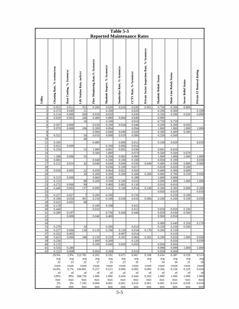
5-5

Table 5-3Reported Maintenance Rates

Uti

lity

Cle

anin

g R

ate,

% s

yste

m/y

ear

Roo

t C

utti

ng, %

Sys

tem

/yr

Lif

t S

tati

on R

ate,

no/

ls/y

r

Flo

w M

onit

orin

g R

ate,

% S

yste

m/y

r

Man

hole

Ins

pect

. % S

yste

m/y

r

Smok

e/dy

e R

ate,

% S

yste

m/y

r

CC

TV

Rat

e, %

Sys

tem

/yr

Pri

vate

Sec

tor

Insp

ecti

on R

ate,

% S

yste

m/y

r

Man

hole

Reh

ab S

tatu

s

Mai

n L

ine

Reh

ab S

tatu

s

Sew

er R

elie

f St

atus

Pri

vate

I/I

Rem

oval

Rat

ing

1 0.052 0.011 353 0.200 0.020 0.010 0.030 0.001 0.750 0.500 0.8002 0.373 0.049 21 0.160 0.020 0.200 0.500 0.1003 0.214 0.000 569 0.020 0.020 0.030 0.330 0.290 0.620 0.6904 0.020 0.003 246 0.400 0.080 0.004 0.040 0.9005 16 0.100 0.010 0.750 0.7506 0.507 0.000 0.034 0.100 0.034 0.046 0.200 0.200 0.0507 0.070 0.000 106 0.200 0.094 0.094 1.000 1.000 1.000 1.0008 0.060 0.040 0.040 0.020 0.300 0.400 0.5009 0.552 50 0.010 0.008 0.010 0.096 0.250 0.500

10 4611 0.185 0.400 0.006 0.012 0.100 0.020 0.01012 0.022 0.009 0.100 0.006 0.01413 0.254 12 1.000 0.001 0.001 0.030 0.001 0.01014 0.500 1.000 0.074 0.560 0.560 0.67015 1.288 0.000 25 0.200 0.002 0.090 1.000 1.000 1.000 1.00016 0.085 0.040 0.100 0.100 0.100 0.050 0.100 0.05017 0.212 0.014 42 0.040 0.040 0.040 0.036 0.040 0.400 0.500 0.800 0.90018 0.036 0.100 0.017 0.020 0.020 0.20019 0.036 0.005 22 0.050 0.064 0.052 0.050 0.400 0.300 0.60020 29 0.200 0.200 0.200 0.200 0.200 0.960 0.700 0.250 0.95021 0.313 0.000 0.060 0.180 0.180 1.000 0.90022 0.155 88 0.200 0.500 0.100 0.016 0.999 1.000 1.000 1.00023 0.272 0.000 99 0.400 0.002 0.130 0.010 0.01024 0.440 0.003 137 0.090 0.422 0.168 0.054 0.140 0.300 0.300 0.600 0.30025 0.050 0.010 0.01026 0.227 0.027 7 0.200 0.100 0.150 0.250 0.10027 0.106 0.054 301 0.150 0.100 0.030 0.016 0.006 0.200 0.200 0.100 0.05028 0.625 0.001 6829 0.119 0.160 0.108 0.02230 0.440 0.010 0.012 0.050 0.050 0.10031 0.289 0.197 0.736 0.436 0.444 0.050 0.030 0.50032 0.000 0.040 0.400 0.900 0.9503334 0.400 0.440 0.350 0.17035 0.270 10 0.200 0.014 0.250 0.250 0.50036 0.227 0.006 130 0.110 0.190 0.120 0.034 0.170 0.200 0.15037 0.352 0.005 0.007 0.014 0.31038 0.623 0.000 348 0.150 0.210 0.202 0.066 0.202 0.200 0.020 1.000 0.95039 0.236 1.000 0.200 0.120 0.050 0.03040 0.125 0.200 0.040 0.050 0.050 0.050 0.05041 0.556 0.280 0.990 0.999 1.000 1.00042 0.322 0.008 0.004 0.200 0.010 0.950 0.600

29.9% 2.9% 123.781 0.205 0.192 0.075 0.067 0.108 0.434 0.387 0.559 0.513avg avg avg avg avg avg avg avg avg avg avg avg32 23 22 27 33 23 35 7 34 36 21 16

count count count count count count count count count count count count24.8% 6.7% 144.801 0.257 0.213 0.099 0.082 0.083 0.366 0.334 0.329 0.434

sd sd sd sd sd sd sd sd sd sd sd sd129% 28% 568.750 1.000 1.000 0.436 0.444 0.202 1.000 1.000 1.000 1.000

max max max max max max max max max max max max2% 0% 7.185 0.004 0.001 0.001 0.010 0.001 0.001 0.010 0.050 0.010

min min min min min min min min min min min min

5-6

Table 5-4

Maintenance Activity Statistics

Activity MeanStandardDeviation Range

Number ofResponses

1. Cleaning, % system/yr 29.9% 24.8% 2% - 129% 32

2. Root removal, % system/yr 2.9% 6.7% 0% - 28% 23

3. Pump station service, no/ps/yr 123.8 144.8 7.2-569 22

4. Flow monitoring, % system/yr 20.5% 25.7% 0.4% - 100% 27

5. Manhole inspection, %system/yr 19.2% 21.3% 0.1% - 100% 33

6. Smoke testing, %system/yr 7.5% 9.9% 0.1% - 43.6% 23

7. CCTV, % system/yr 6.7% 8.2% 1.0% - 44.4% 35

8. Private sector inspections, % system/yr 10.8% 8.3% 0.1% - 20.2% 7

9. Manhole rehabilitation, % complete 43.4% 36.6% 0.1% - 100% 34

10. Main line rehabilitation, % complete 38.7% 33.4% 0.1% - 100% 36

11. Relief construction, % complete 55.9% 32.9% 5% - 100% 21

12. Private sector I/I removal, % complete 51.3% 43.3% 0.1% - 100% 16

The relationship between maintenance activity rate and maintenance frequency was

determined by setting a maintenance frequency of 10 percent equal to the mean value for each

maintenance activity and assigning corresponding maintenance frequencies on either side of the

mean based on the area under the normal curve. The selection of 10 percent maintenance

frequency association with the mean maintenance rate assumes that on average, most systems will

perform 100 percent of maintenance activities in a 10 year period. The maintenance frequencies

assigned to each deviation from the mean are shown on Figure 5-1.

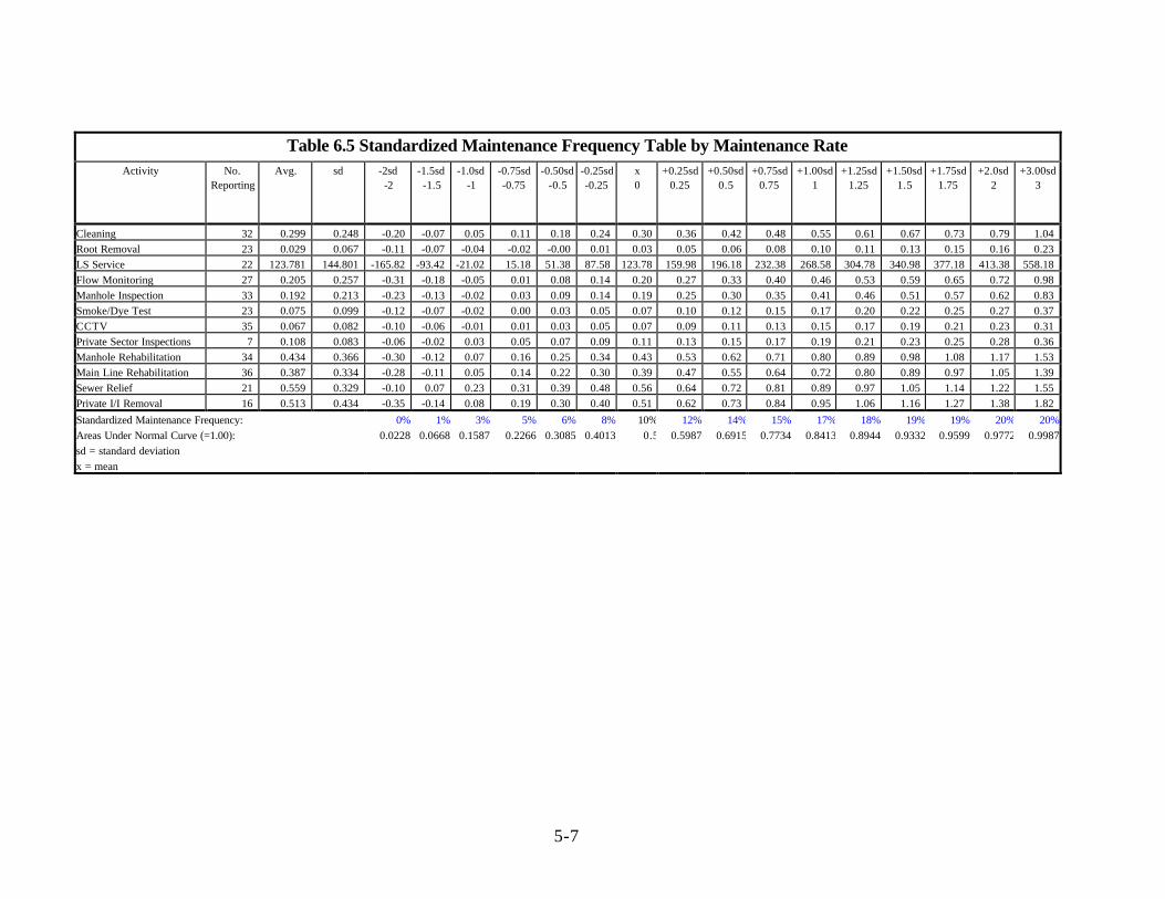
5-7

Table 6.5 Standardized Maintenance Frequency Table by Maintenance RateActivity No.

ReportingAvg. sd -2sd

-2-1.5sd-1.5

-1.0sd-1

-0.75sd-0.75

-0.50sd-0.5

-0.25sd-0.25

x0

+0.25sd0.25

+0.50sd0.5

+0.75sd0.75

+1.00sd1

+1.25sd1.25

+1.50sd1.5

+1.75sd1.75

+2.0sd2

+3.00sd3

Cleaning 32 0.299 0.248 -0.20 -0.07 0.05 0.11 0.18 0.24 0.30 0.36 0.42 0.48 0.55 0.61 0.67 0.73 0.79 1.04

Root Removal 23 0.029 0.067 -0.11 -0.07 -0.04 -0.02 -0.00 0.01 0.03 0.05 0.06 0.08 0.10 0.11 0.13 0.15 0.16 0.23

LS Service 22 123.781 144.801 -165.82 -93.42 -21.02 15.18 51.38 87.58 123.78 159.98 196.18 232.38 268.58 304.78 340.98 377.18 413.38 558.18

Flow Monitoring 27 0.205 0.257 -0.31 -0.18 -0.05 0.01 0.08 0.14 0.20 0.27 0.33 0.40 0.46 0.53 0.59 0.65 0.72 0.98

Manhole Inspection 33 0.192 0.213 -0.23 -0.13 -0.02 0.03 0.09 0.14 0.19 0.25 0.30 0.35 0.41 0.46 0.51 0.57 0.62 0.83

Smoke/Dye Test 23 0.075 0.099 -0.12 -0.07 -0.02 0.00 0.03 0.05 0.07 0.10 0.12 0.15 0.17 0.20 0.22 0.25 0.27 0.37

CCTV 35 0.067 0.082 -0.10 -0.06 -0.01 0.01 0.03 0.05 0.07 0.09 0.11 0.13 0.15 0.17 0.19 0.21 0.23 0.31

Private Sector Inspections 7 0.108 0.083 -0.06 -0.02 0.03 0.05 0.07 0.09 0.11 0.13 0.15 0.17 0.19 0.21 0.23 0.25 0.28 0.36

Manhole Rehabilitation 34 0.434 0.366 -0.30 -0.12 0.07 0.16 0.25 0.34 0.43 0.53 0.62 0.71 0.80 0.89 0.98 1.08 1.17 1.53

Main Line Rehabilitation 36 0.387 0.334 -0.28 -0.11 0.05 0.14 0.22 0.30 0.39 0.47 0.55 0.64 0.72 0.80 0.89 0.97 1.05 1.39

Sewer Relief 21 0.559 0.329 -0.10 0.07 0.23 0.31 0.39 0.48 0.56 0.64 0.72 0.81 0.89 0.97 1.05 1.14 1.22 1.55

Private I/I Removal 16 0.513 0.434 -0.35 -0.14 0.08 0.19 0.30 0.40 0.51 0.62 0.73 0.84 0.95 1.06 1.16 1.27 1.38 1.82

Standardized Maintenance Frequency: 0% 1% 3% 5% 6% 8% 10% 12% 14% 15% 17% 18% 19% 19% 20% 20%

Areas Under Normal Curve (=1.00): 0.0228 0.0668 0.1587 0.2266 0.3085 0.4013 0.5 0.5987 0.6915 0.7734 0.8413 0.8944 0.9332 0.9599 0.9772 0.9987

sd = standard deviation

x = mean

5-8

Figure 5-1 Maintenance Frequency Assignments

5.4 Determination of Maintenance Frequency

An overall maintenance frequency for each agency was determined by applying the actual

maintenance rates reported from Table 5-3, the relative weight for each maintenance activity from

Table 5-1, and the corresponding standard activity maintenance frequency using Table 5-5.

Average maintenance activity rates were used for missing data to estimate the maintenance

frequency for each agency. The range and mean of the maintenance frequencies derived is

presented in Table 5-6 and shown on the distribution curve on

Figure 5-2. The system maintenance frequency determined for each agency is presented in Table

5-7.

Measured Maintenance Frequency

.12.10.08.06.04.02

Pre

dict

ed M

aint

enan

ce F

requ

ency

.10

.08

.06

.04

.02

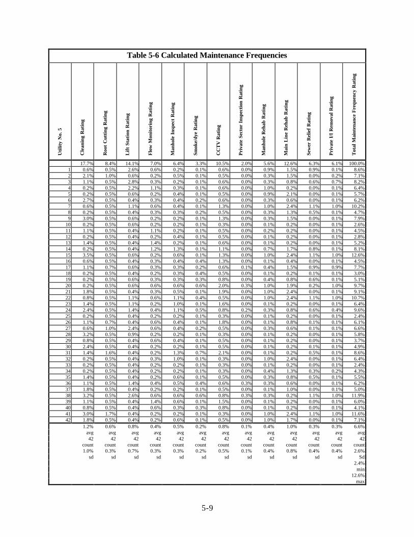
5-9

Table 5-6 Calculated Maintenance FrequenciesU

tili

ty N

o. 5

Cle

anin

g R

atin

g

Roo

t C

utti

ng R

atin

g

Lif

t S

tati

on R

atin

g

Flo

w M

onit

orin

g R

atin

g

Man

hole

Ins

pect

Rat

ing

Smok

e/dy

e R

atin

g

CC

TV

Rat

ing

Pri

vate

Sec

tor

Insp

ecti

on R

atin

g

Man

hole

Reh

ab R

atin

g

Mai

n L

ine

Reh

ab R

atin

g

Sew

er R

elie

f R

atin

g

Pri

vate

I/I

Rem

oval

Rat

ing

Tot

al M

aint

enan

ce F

requ

ency

Rat

ing

17.7% 8.4% 14.1% 7.0% 6.4% 3.3% 10.5% 2.0% 5.6% 12.6% 6.3% 6.1% 100.0%1 0.6% 0.5% 2.6% 0.6% 0.2% 0.1% 0.6% 0.0% 0.9% 1.5% 0.9% 0.1% 8.6%2 2.1% 1.0% 0.6% 0.2% 0.5% 0.1% 0.5% 0.0% 0.3% 1.5% 0.0% 0.2% 7.1%3 1.1% 0.5% 2.8% 0.3% 0.2% 0.1% 0.6% 0.0% 0.3% 0.8% 0.6% 0.7% 8.2%4 0.2% 0.5% 2.2% 1.1% 0.3% 0.1% 0.6% 0.0% 1.0% 0.2% 0.0% 0.1% 6.4%5 0.2% 0.5% 0.6% 0.2% 0.4% 0.1% 0.5% 0.0% 0.9% 2.1% 0.0% 0.1% 5.7%6 2.7% 0.5% 0.4% 0.3% 0.4% 0.2% 0.6% 0.0% 0.3% 0.6% 0.0% 0.1% 6.2%7 0.6% 0.5% 1.1% 0.6% 0.4% 0.1% 1.3% 0.0% 1.0% 2.4% 1.1% 1.0% 10.2%8 0.2% 0.5% 0.4% 0.3% 0.3% 0.2% 0.5% 0.0% 0.3% 1.3% 0.5% 0.1% 4.7%9 3.0% 0.5% 0.6% 0.2% 0.2% 0.1% 1.3% 0.0% 0.3% 1.5% 0.0% 0.1% 7.9%

10 0.2% 0.5% 0.6% 0.2% 0.2% 0.1% 0.3% 0.0% 0.1% 0.2% 0.0% 0.1% 2.6%11 1.1% 0.5% 0.4% 1.1% 0.2% 0.1% 0.5% 0.0% 0.2% 0.2% 0.0% 0.1% 4.5%12 0.2% 0.5% 0.4% 0.2% 0.4% 0.1% 0.5% 0.0% 0.1% 0.2% 0.0% 0.1% 2.8%13 1.4% 0.5% 0.4% 1.4% 0.2% 0.1% 0.6% 0.0% 0.1% 0.2% 0.0% 0.1% 5.2%14 0.2% 0.5% 0.4% 1.2% 1.3% 0.1% 1.1% 0.0% 0.7% 1.7% 0.8% 0.1% 8.1%15 3.5% 0.5% 0.6% 0.2% 0.6% 0.1% 1.3% 0.0% 1.0% 2.4% 1.1% 1.0% 12.6%16 0.6% 0.5% 0.4% 0.3% 0.4% 0.4% 1.3% 0.0% 0.1% 0.4% 0.0% 0.1% 4.5%17 1.1% 0.7% 0.6% 0.3% 0.3% 0.2% 0.6% 0.1% 0.4% 1.5% 0.9% 0.9% 7.7%18 0.2% 0.5% 0.4% 0.2% 0.3% 0.4% 0.5% 0.0% 0.1% 0.2% 0.1% 0.1% 3.0%19 0.2% 0.5% 0.6% 0.3% 0.3% 0.3% 0.8% 0.0% 0.4% 0.8% 0.6% 0.1% 5.1%20 0.2% 0.5% 0.6% 0.6% 0.6% 0.6% 2.0% 0.3% 1.0% 1.9% 0.2% 1.0% 9.7%21 1.8% 0.5% 0.4% 0.3% 0.5% 0.1% 1.9% 0.0% 1.0% 2.4% 0.0% 0.1% 9.1%22 0.8% 0.5% 1.1% 0.6% 1.1% 0.4% 0.5% 0.0% 1.0% 2.4% 1.1% 1.0% 10.7%23 1.4% 0.5% 1.1% 0.2% 1.0% 0.1% 1.6% 0.0% 0.1% 0.2% 0.0% 0.1% 6.4%24 2.4% 0.5% 1.4% 0.4% 1.1% 0.5% 0.8% 0.2% 0.3% 0.8% 0.6% 0.4% 9.6%25 0.2% 0.5% 0.4% 0.2% 0.2% 0.1% 0.3% 0.0% 0.1% 0.2% 0.0% 0.1% 2.4%26 1.1% 0.7% 0.4% 0.6% 0.4% 0.1% 1.8% 0.0% 0.1% 0.8% 0.1% 0.1% 6.1%27 0.6% 1.0% 2.4% 0.6% 0.4% 0.2% 0.5% 0.0% 0.3% 0.6% 0.1% 0.1% 6.6%28 3.2% 0.5% 0.9% 0.2% 0.2% 0.1% 0.3% 0.0% 0.1% 0.2% 0.0% 0.1% 5.8%29 0.8% 0.5% 0.4% 0.6% 0.4% 0.1% 0.5% 0.0% 0.1% 0.2% 0.0% 0.1% 3.7%30 2.4% 0.5% 0.4% 0.2% 0.2% 0.1% 0.5% 0.0% 0.1% 0.2% 0.1% 0.1% 4.9%31 1.4% 1.6% 0.4% 0.2% 1.3% 0.7% 2.1% 0.0% 0.1% 0.2% 0.5% 0.1% 8.6%32 0.2% 0.5% 0.4% 0.3% 1.0% 0.1% 0.3% 0.0% 1.0% 2.4% 0.0% 0.1% 6.4%33 0.2% 0.5% 0.4% 0.2% 0.2% 0.1% 0.3% 0.0% 0.1% 0.2% 0.0% 0.1% 2.4%34 0.2% 0.5% 0.4% 0.2% 0.2% 0.1% 0.3% 0.0% 0.4% 1.3% 0.3% 0.2% 4.3%35 1.4% 0.5% 0.4% 0.2% 0.6% 0.1% 0.5% 0.0% 0.3% 0.8% 0.5% 0.1% 5.5%36 1.1% 0.5% 1.4% 0.4% 0.5% 0.4% 0.6% 0.3% 0.3% 0.6% 0.0% 0.1% 6.2%37 1.8% 0.5% 0.4% 0.2% 0.2% 0.1% 0.5% 0.0% 0.1% 1.0% 0.0% 0.1% 5.0%38 3.2% 0.5% 2.6% 0.6% 0.6% 0.6% 0.8% 0.3% 0.3% 0.2% 1.1% 1.0% 11.9%39 1.1% 0.5% 0.4% 1.4% 0.6% 0.1% 1.5% 0.0% 0.1% 0.2% 0.0% 0.1% 6.0%40 0.8% 0.5% 0.4% 0.6% 0.3% 0.3% 0.8% 0.0% 0.1% 0.2% 0.0% 0.1% 4.1%41 3.0% 1.7% 0.4% 0.2% 0.2% 0.1% 0.3% 0.0% 1.0% 2.4% 1.1% 1.0% 11.6%42 1.8% 0.5% 0.4% 0.2% 0.6% 0.1% 0.5% 0.0% 1.0% 1.7% 0.0% 0.1% 7.1%

1.2% 0.6% 0.8% 0.4% 0.5% 0.2% 0.8% 0.1% 0.4% 1.0% 0.3% 0.3% 6.6%avg avg avg avg avg avg avg avg avg avg avg avg avg42 42 42 42 42 42 42 42 42 42 42 42 42

count count count count count count count count count count count count count1.0% 0.3% 0.7% 0.3% 0.3% 0.2% 0.5% 0.1% 0.4% 0.8% 0.4% 0.4% 2.6%

sd sd sd sd sd sd sd sd sd sd sd sd Sd2.4%min

12.6%max

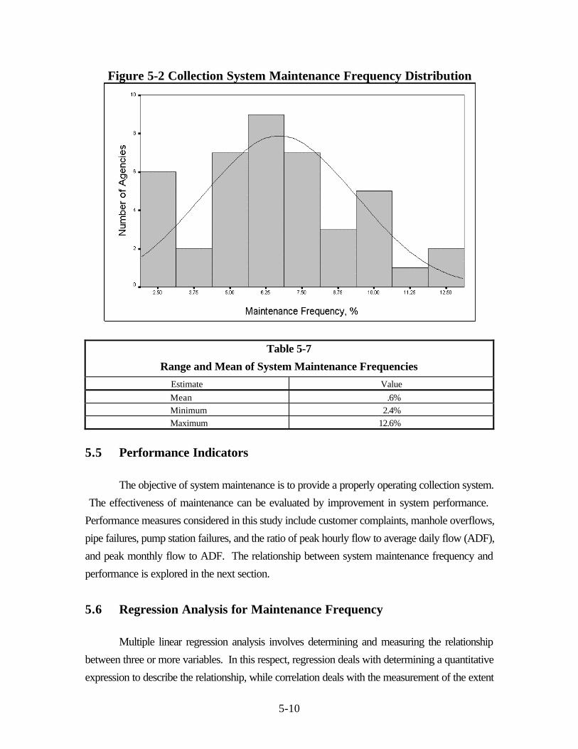
5-10

Figure 5-2 Collection System Maintenance Frequency Distribution

Table 5-7

Range and Mean of System Maintenance Frequencies

Estimate Value

Mean .6%

Minimum 2.4%

Maximum 12.6%

5.5 Performance Indicators

The objective of system maintenance is to provide a properly operating collection system.

The effectiveness of maintenance can be evaluated by improvement in system performance.

Performance measures considered in this study include customer complaints, manhole overflows,

pipe failures, pump station failures, and the ratio of peak hourly flow to average daily flow (ADF),

and peak monthly flow to ADF. The relationship between system maintenance frequency and

performance is explored in the next section.

5.6 Regression Analysis for Maintenance Frequency

Multiple linear regression analysis involves determining and measuring the relationship

between three or more variables. In this respect, regression deals with determining a quantitative

expression to describe the relationship, while correlation deals with the measurement of the extent

5-11

of the relationship. Linear regression is a procedure of estimating a linear relationship between a

dependent variable, and one or more independent variables. The general form of a multiple

regression equation is:

Y= B1 + B2X1 + ..........BnXn-1 +e

Where:

Y = dependent variable

Xi = ith independent variable for I=1...n

Bi = ith coefficient for Xi

e = random error

The variable Ae@ is a random error parameter and is assumed to have a normal distribution with a

mean of zero and a constant variance for all values of independent variables. The multiple

regression used in the model building process uses the least square method to estimate the

coefficients. All regression analyses were performed using the SPSS statistical software package

for Windows Release 6.0 .

Regression analyses were performed using the derived maintenance frequency as the

dependent variable and various sets of independent variables. The purpose of this analysis was to

explore the relationship, if any, between calculated maintenance frequency and key independent

variables, including performance measures, the number of pump stations, the size of the agency, and

the regional location of the agency, which may tend to result in the need for maintenance. The

independent variables considered for analysis, were selected from the list of data requested from

the agencies and are summarized in Table 5-8.

5-12

Table 5-8

Potential Independent Variables Related to Maintenance Frequency

Variable Unit Code

Customer Complaints - last 5 years Complaints/mile$year CUSTC_5

Manhole and Treatment Overflows last 5years

Overflows/mile$year MHOF_5

Pipe Failures - last 5 years Failures/mile$year PIPEF_5

Pump Station Failures - last 5 years Failures/pump station$year PSF_5

Pump Station Number Number of pump stations PS_NO

Size of Agency Based on size designation - small, medium,large

SIZE_CD

Location of Agency Based on regional codes established for thisproject

REG_CD

Ratio of Peak Hourly Flow to Annual AverageFlow

Ratio PH_ADF

Ratio of Peak Monthly Flow to AnnualAverage Flow

Ratio PM_ADF

Note: The code is used in the SPSS statistical software package and is listed here for reference.

A number of regression analyses were performed to evaluate possible relationships. Out

of the many analyses performed, nine are documented in this report. The coefficients of

determination (R2) for the nine documented analyses are presented in Table 5-9. The analyses

show that the best R2 is obtained when all nine independent variables are considered. The R2

values show that the estimate of the maintenance frequency is highly dependent on customer

complaints, manhole overflows, size characteristics, regional characteristics, peak hour/ADF ratio,

and pump station failure rates. The Size Code is 1 = small, 2 = medium, 3 = large, and the

Regional Code is 1 = central, 2 = northeast, 3 = northwest, 4 = southeast, and 5 = southwest. The

regression equation coefficients for the four best relationships (R2 greater than 0.80) are presented

in Table 5-10. These regression coefficients were used to estimate the maintenance frequency from

those agencies that provided complete information. Only 12 agencies provided all the data

necessary for the regression analysis. The results presented on Figure 5-3 show good agreement

between the calculated (from Table 5-7) and the predicted maintenance frequency using Equation

MF1 in Table 5-10. The results on Figure 5-3 indicate that system performance measures and

system maintenance frequencies may be related.

5-13

Table 5-9

Regression Analysis for Maintenance Frequency

Independent VariablesCoefficient ofDetermination

No.Var C

usto

mer

Com

plai

nts

Man

hole

Ove

rflo

ws

Pip

e F

ailu

res

Siz

e C

ode

Reg

ion

Cod

e

Pea

k H

our/

AD

F

Pea

k M

onth

/AD

F

Pum

p S

tatio

n F

ailu

re

Pum

p S

tati

on Q

uant

ity

R2

Adj

uste

d R

2 (1

)

SelectedRegressionAnalysesR2>0.80

EquationName

9 X X X X X X X X X 0.975 0.863 X MF1

8 X X X X X X X X 0.896 0.619 X MF2

7 X X X X X X X 0.827 0.523 X MF3

7 X X X X X X X 0.495 0.053

6 X X X X X X 0.593 0.276

6 X X X X X X 0.609 0.140

6 X X X X X X 0.318 -0.054

6 X X X X X X 0.639 0.422

6 X X X X X X 0.826 0.618 X MF5(1) The adjusted R2 statistic attempts to model R2 to more closely reflect the goodness of fit of the model inthe population. (pg. 318 SPSS Manual)

1P-N-

)R-(1 P -R = R

222

Table 5-10

Regression Coefficients for Maintenance Frequencies

Linear Regression Equation CoefficientsItem

Equation MF1 Equation MF2 Equation MF3 Equation MF4

Constant -0.107 -0.123 0.0796 0.0804

Customer Complaints -0.0484 -.00041 -0.00156 0.00152

Manhole Overflows -0.340 -0.139 -0.190 -0.189

Pipe Failures -0.422 -0.0760 -0.00359 ----

Size Code -0.00978 -0.0103 -0.00658 -0.0065

Region Code -0.0129 0.0031 0.00849 0.00841

Peak Hour/ADF -0.0920 -0.0093 -0.000785 -0.001

Peak Month/ADF 0.430 ---- ---- ---

Pump Station Failure 0.344 -0.839 -0.826 -0.828

Pump Station Number 0.00004 0.000038 ---- ----

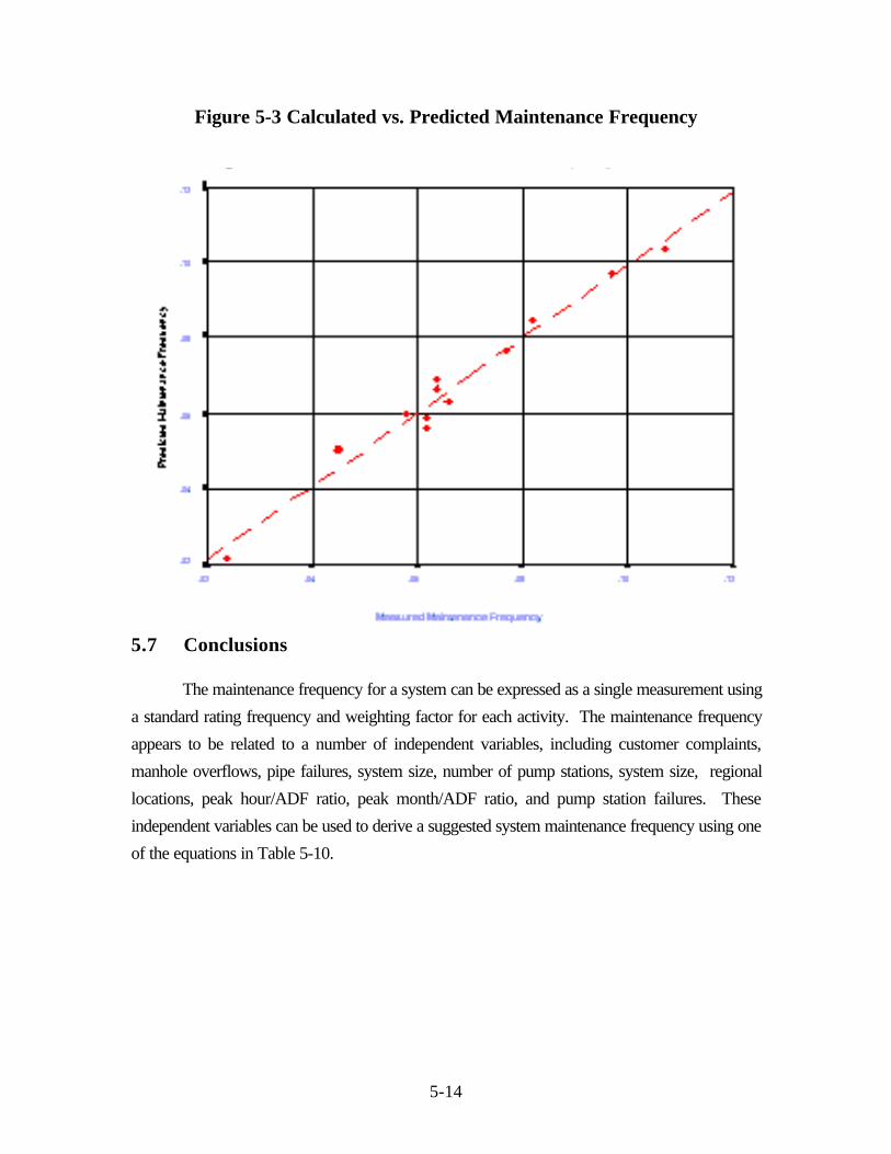
5-14

Figure 5-3 Calculated vs. Predicted Maintenance Frequency

5.7 Conclusions

The maintenance frequency for a system can be expressed as a single measurement using

a standard rating frequency and weighting factor for each activity. The maintenance frequency

appears to be related to a number of independent variables, including customer complaints,

manhole overflows, pipe failures, system size, number of pump stations, system size, regional

locations, peak hour/ADF ratio, peak month/ADF ratio, and pump station failures. These

independent variables can be used to derive a suggested system maintenance frequency using one

of the equations in Table 5-10.

6-1

6.0 Determination of System Performance Rating

6.1 Introduction

System performance measurements should indicate how well or how poorly a collection

system is providing the intended service. The measurement of system performance is crucial to the

optimization of maintenance, for without a proper Ayardstick@, it is not possible to tell how effective

the maintenance program is. All performance measures are not necessarily equal in importance.

Therefore, when evaluating an agency=s performance, the most important question is how the

system as a whole is performing based on a number of significant factors. It does little good for an

agency to have zero pipe failures and yet have a large number of complaints about sewage backing

up into homes. Just as with maintenance activities, an effective performance evaluation requires

consideration of a number of factors. This chapter presents the evaluation of performance, the

determination of a performance rating for the agencies surveyed, and the procedures to follow in

determining the performance rating.

6.2 Performance Data Weighting

In order to develop an overall performance rating, each agency was requested to provide

its opinion of the relative importance of six commonly used collection system performance measures

as described below:

Pipe Failure - a pipe which has lost its structural integrity as evidenced by total or partial

collapse (loss of 50% of pipe area or 25% of pipe wall around any circumference.

Measured by failures per mile per year.

Sanitary Sewer Overflow (SSO) - a discharge of wastewater from the collection system

with the potential to enter surface water courses occurring either in the collection system

or in the headworks of the wastewater treatment plant.

Complaints - a customer complaint related to the performance of the collection system,

including issues such as overflows, odors, and loose manhole covers.

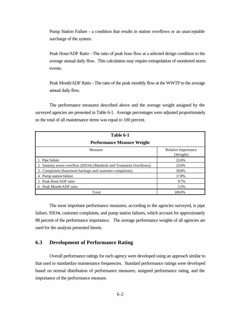
6-2

Pump Station Failure - a condition that results in station overflows or an unacceptable

surcharge of the system.

Peak Hour/ADF Ratio - The ratio of peak hour flow at a selected design condition to the

average annual daily flow. This calculation may require extrapolation of monitored storm

events.

Peak Month/ADF Ratio - The ratio of the peak monthly flow at the WWTP to the average

annual daily flow.

The performance measures described above and the average weight assigned by the

surveyed agencies are presented in Table 6-1. Average percentages were adjusted proportionately

so the total of all maintenance items was equal to 100 percent.

Table 6-1

Performance Measure Weight

Measure Relative Importance(Weight)

1. Pipe failure 22.6%

2. Sanitary sewer overflow (SSO=s) (Manhole and Treatment Overflows) 23.6%

3. Complaints (basement backups and customer complaints) 20.8%

4. Pump station failure 17.8%

5. Peak Hour/ADF ratio 9.7%

6. Peak Month/ADF ratio 5.5%

Total 100.0%

The most important performance measures, according to the agencies surveyed, is pipe

failure, SSO=s, customer complaints, and pump station failures, which account for approximately

88 percent of the performance importance. The average performance weights of all agencies are

used for the analysis presented herein.

6.3 Development of Performance Rating

Overall performance ratings for each agency were developed using an approach similar to

that used to standardize maintenance frequencies. Standard performance ratings were developed

based on normal distribution of performance measures, assigned performance rating, and the

importance of the performance measure.

6-3

6.3.1 Determining Performance RatingAll performance measures were converted into unit rates, such as pipe failures per mile per

year. Performance measures over the past 5 years were used as the basis for the analysis, since

this data period provided more complete information than longer periods. Performance data for

each agency is presented in Table 6-2. Blank cells indicate that the data was not provided by the

agency. Performance rates for each agency were determined using the performance data and

appropriate measures, such as miles of sewer. To determine performance, adjustments to miles

of sewer were made based on the age information provided by each agency to more accurately

estimate the true rate of each performance data. The performance rates for each agency are

presented in Table 6-3.

6.3.2 Developing the Standard RatingThe mean, standard deviation, range, and number of responses for each performance

measure are listed in Table 6-4. The rate of each performance measure was then normalized using

the normal distribution to develop a standard by which any performance rate, or group of

performance rates from various performance measures could be compared. Once the performance

data was normalized, a standard performance rating was assigned to selected deviations from the

mean. The assignment of the standard performance rating was somewhat arbitrary; however,

based on the initial hypothesis, an average rating of 65 to 75% for the age of the systems

investigated was assumed to be reasonable. Through trial and error, an average performance rating

of 71.1% was determined, as discussed in more detail in Section 6.4. The standardized

performance ratings assigned to each deviation from the mean for each performance measured data

are given in Table 6-5. The weights used for analysis are also given in Table 6-5. It should be

noted that the performance weight suggested by agencies for complaints was split 50/50 between

basement backups and customer complaints.

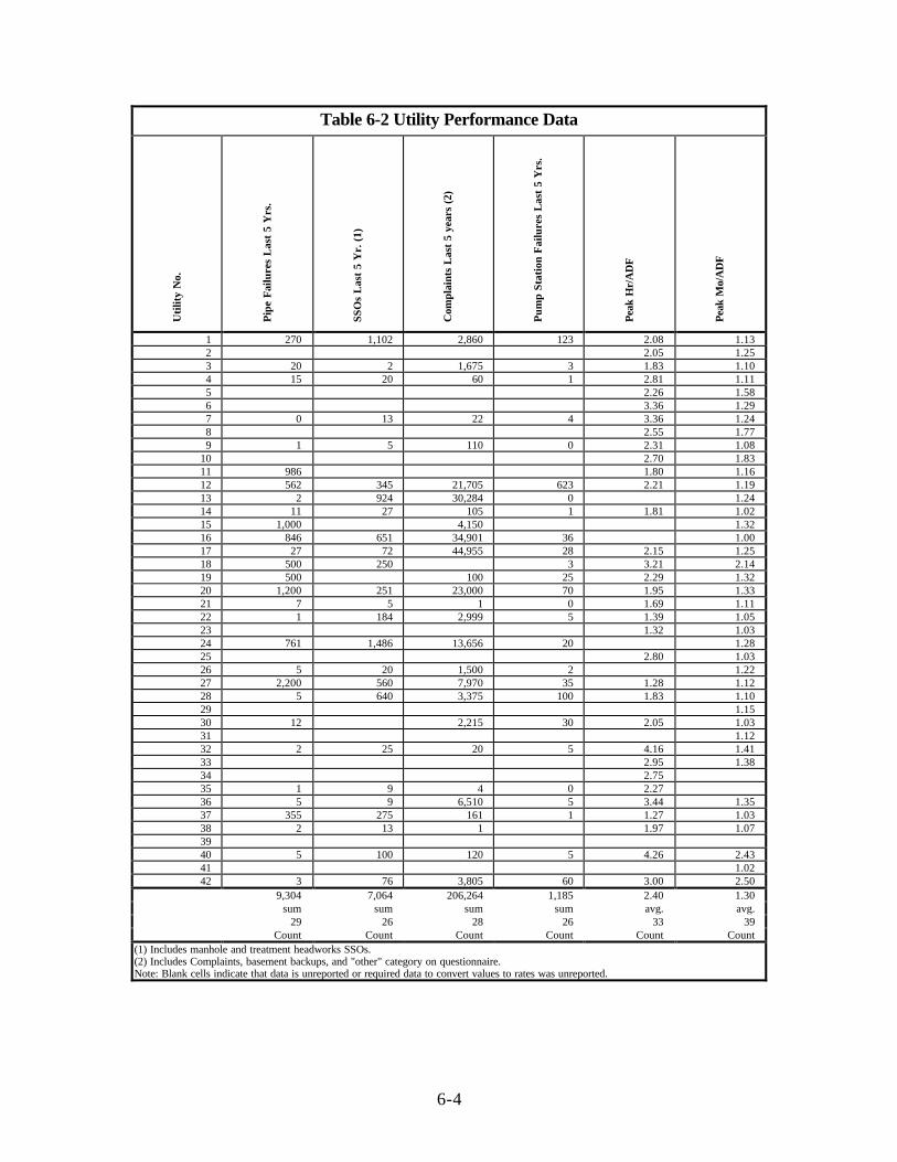
6-4

Table 6-2 Utility Performance Data

Uti

lity

No.

Pip

e F

ailu

res

Las

t 5

Yrs

.

SSO

s L

ast

5 Y

r. (

1)

Com

plai

nts

Las

t 5

year

s (2

)

Pum

p St

atio

n F

ailu

res

Las

t 5

Yrs

.

Pea

k H

r/A

DF

Pea

k M

o/A

DF

1 270 1,102 2,860 123 2.08 1.132 2.05 1.253 20 2 1,675 3 1.83 1.104 15 20 60 1 2.81 1.115 2.26 1.586 3.36 1.297 0 13 22 4 3.36 1.248 2.55 1.779 1 5 110 0 2.31 1.08

10 2.70 1.8311 986 1.80 1.1612 562 345 21,705 623 2.21 1.1913 2 924 30,284 0 1.2414 11 27 105 1 1.81 1.0215 1,000 4,150 1.3216 846 651 34,901 36 1.0017 27 72 44,955 28 2.15 1.2518 500 250 3 3.21 2.1419 500 100 25 2.29 1.3220 1,200 251 23,000 70 1.95 1.3321 7 5 1 0 1.69 1.1122 1 184 2,999 5 1.39 1.0523 1.32 1.0324 761 1,486 13,656 20 1.2825 2.80 1.0326 5 20 1,500 2 1.2227 2,200 560 7,970 35 1.28 1.1228 5 640 3,375 100 1.83 1.1029 1.1530 12 2,215 30 2.05 1.0331 1.1232 2 25 20 5 4.16 1.4133 2.95 1.3834 2.7535 1 9 4 0 2.2736 5 9 6,510 5 3.44 1.3537 355 275 161 1 1.27 1.0338 2 13 1 1.97 1.073940 5 100 120 5 4.26 2.4341 1.0242 3 76 3,805 60 3.00 2.50

9,304 7,064 206,264 1,185 2.40 1.30sum sum sum sum avg. avg.

29 26 28 26 33 39Count Count Count Count Count Count

(1) Includes manhole and treatment headworks SSOs.(2) Includes Complaints, basement backups, and "other" category on questionnaire.Note: Blank cells indicate that data is unreported or required data to convert values to rates was unreported.

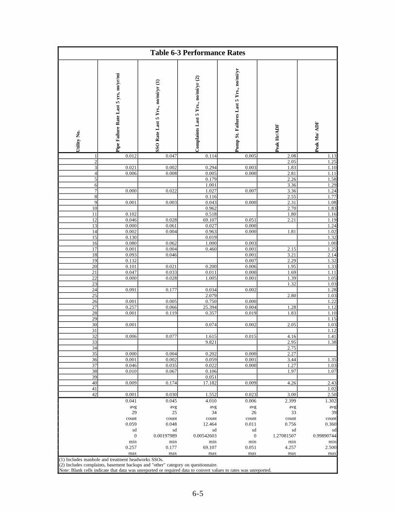
6-5

Table 6-3 Performance Rates

Uti

lity

No.

Pip

e F

ailu

re R

ate

Las

t 5

yrs,

no/

yr/m

i

SSO

Rat

e L

ast

5 Y

rs.,

no/m

i/yr

(1)

Com

plai

nts

Las

t 5

Yrs

., no

/mi/y

r (2

)

Pum

p St

. Fai

lure

s L

ast

5 Y

rs.,

no/m

i/yr

Pea

k H

r/A

DF

Pea

k M

o/ A

DF

1 0.012 0.047 0.114 0.005 2.08 1.132 2.05 1.253 0.021 0.002 0.294 0.003 1.83 1.104 0.006 0.008 0.005 0.000 2.81 1.115 0.179 2.26 1.586 1.001 3.36 1.297 0.000 0.022 1.027 0.007 3.36 1.248 0.116 2.55 1.779 0.001 0.003 0.043 0.000 2.31 1.08

10 0.962 2.70 1.8311 0.102 0.518 1.80 1.1612 0.046 0.028 69.107 0.051 2.21 1.1913 0.000 0.061 0.027 0.000 1.2414 0.002 0.004 0.963 0.000 1.81 1.0215 0.130 0.019 1.3216 0.080 0.062 1.000 0.003 1.0017 0.001 0.004 0.460 0.001 2.15 1.2518 0.093 0.046 0.001 3.21 2.1419 0.132 0.007 2.29 1.3220 0.101 0.021 0.200 0.006 1.95 1.3321 0.047 0.033 0.011 0.000 1.69 1.1122 0.000 0.028 1.005 0.001 1.39 1.0523 1.32 1.0324 0.091 0.177 0.034 0.002 1.2825 2.079 2.80 1.0326 0.001 0.005 0.750 0.000 1.2227 0.257 0.066 25.394 0.004 1.28 1.1228 0.001 0.119 0.357 0.019 1.83 1.1029 1.1530 0.001 0.074 0.002 2.05 1.0331 1.1232 0.006 0.077 1.615 0.015 4.16 1.4133 9.821 2.95 1.3834 2.7535 0.000 0.004 0.202 0.000 2.2736 0.001 0.002 0.059 0.001 3.44 1.3537 0.046 0.035 0.022 0.000 1.27 1.0338 0.010 0.067 0.106 1.97 1.0739 0.05140 0.009 0.174 17.182 0.009 4.26 2.4341 1.0242 0.001 0.030 1.552 0.023 3.00 2.50

0.041 0.045 4.010 0.006 2.399 1.302avg avg avg avg avg avg29 25 34 26 33 39

count count count count count count0.059 0.048 12.464 0.011 0.756 0.360

sd sd sd sd sd sd0 0.00197989 0.00542603 0 1.27081507 0.99890744

min min min min min min0.257 0.177 69.107 0.051 4.257 2.500

max max max max max max(1) Includes manhole and treatment headworks SSOs.(2) Includes complaints, basement backups and "other" category on questionnaire.Note: Blank cells indicate that data was unreported or required data to convert values to rates was unreported.

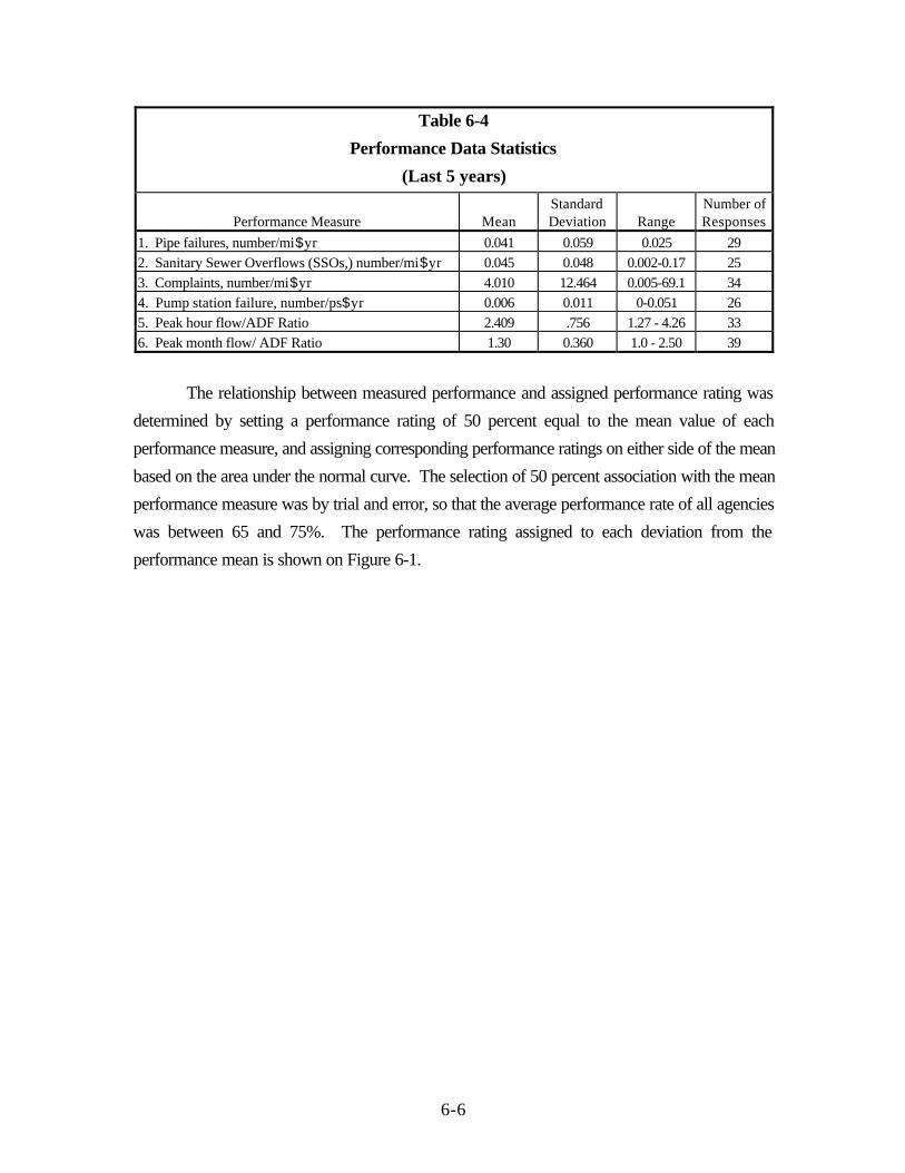
6-6

Table 6-4

Performance Data Statistics

(Last 5 years)

Performance Measure MeanStandardDeviation Range

Number ofResponses

1. Pipe failures, number/mi$yr 0.041 0.059 0.025 29

2. Sanitary Sewer Overflows (SSOs,) number/mi$yr 0.045 0.048 0.002-0.17 25

3. Complaints, number/mi$yr 4.010 12.464 0.005-69.1 34

4. Pump station failure, number/ps$yr 0.006 0.011 0-0.051 26

5. Peak hour flow/ADF Ratio 2.409 .756 1.27 - 4.26 33

6. Peak month flow/ ADF Ratio 1.30 0.360 1.0 - 2.50 39

The relationship between measured performance and assigned performance rating was

determined by setting a performance rating of 50 percent equal to the mean value of each

performance measure, and assigning corresponding performance ratings on either side of the mean

based on the area under the normal curve. The selection of 50 percent association with the mean

performance measure was by trial and error, so that the average performance rate of all agencies

was between 65 and 75%. The performance rating assigned to each deviation from the

performance mean is shown on Figure 6-1.

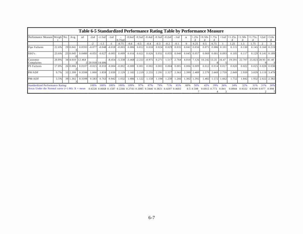
6-7

Table 6-5 Standardized Performance Rating Table by Performance MeasurePerformance Measure Weigh

tNo. Avg. sd -2sd -1.5sd -1sd -

0.75sd-0.6sd -0.5sd -0.4sd -0.3sd -0.2sd -.1sd x +.25s

d+0.50s

d+.75s

d+1sd +1.25s

d+1.50s

d+1.75s

d+2sd +3.0s

d

-2 -1.5 -1 -0.75 -0.6 -0.5 -0.4 -0.3 -0.2 -0.1 0 0.25 0.5 0.75 1 1.25 1.5 1.75 2 3Pipe Failures 22.6% 29 0.041

30.0593 -0.077 -0.048 -0.018 -0.003 0.006 0.012 0.018 0.024 0.029 0.035 0.041 0.056 0.071 0.086 0.101 0.115 0.130 0.145 0.160 0.219

SSO's 23.6% 25 0.0450

0.0480 -0.051 -0.027 -0.003 0.009 0.016 0.021 0.026 0.031 0.035 0.040 0.045 0.057 0.069 0.081 0.093 0.105 0.117 0.129 0.141 0.189

CustomerComplaints

20.8% 34 4.0103

12.4642

-20.918

-14.686

-8.454 -5.338 -3.468 -2.222 -0.975 0.271 1.517 2.764 4.010 7.126 10.242 13.358

16.475

19.591 22.707 25.823 28.939

41.403

PS Failures 17.8% 26 0.0062

0.0107 -0.015 -0.010 -0.004 -0.002 -0.000 0.001 0.002 0.003 0.004 0.005 0.006 0.009 0.012 0.014 0.017 0.020 0.022 0.025 0.028 0.038

PH/ADF 9.7% 33 2.3992

0.3598 1.000 1.859 2.039 2.129 2.183 2.219 2.255 2.291 2.327 2.363 2.399 2.489 2.579 2.669 2.759 2.849 2.939 3.029 3.119 3.479

PM/ADF 5.5% 39 1.3023

0.3598 0.583 0.763 0.942 1.032 1.086 1.122 1.158 1.194 1.230 1.266 1.302 1.392 1.482 1.572 1.662 1.752 1.842 1.932 2.022 2.382

100% 100% 100% 100% 109% 97% 87% 79% 71% 65% 60% 50% 43% 39% 36% 34% 32% 31% 31% 30%Standardized Performance Rating:Areas Under the Normal curve (+1.00): X = mean 0.0228 0.0668 0.1587 0.2266 0.2743 0.3085 0.3446 0.3821 0.4207 0.4602 0.5 0.598

70.6915 0.773

40.841

30.8944 0.9332 0.9599 0.977

20.998

7

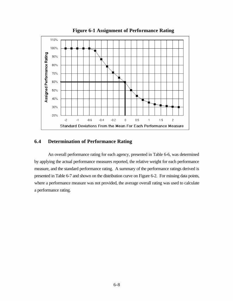
6-8

Figure 6-1 Assignment of Performance Rating

6.4 Determination of Performance Rating

An overall performance rating for each agency, presented in Table 6-6, was determined

by applying the actual performance measures reported, the relative weight for each performance

measure, and the standard performance rating. A summary of the performance ratings derived is

presented in Table 6-7 and shown on the distribution curve on Figure 6-2. For missing data points,

where a performance measure was not provided, the average overall rating was used to calculate

a performance rating.

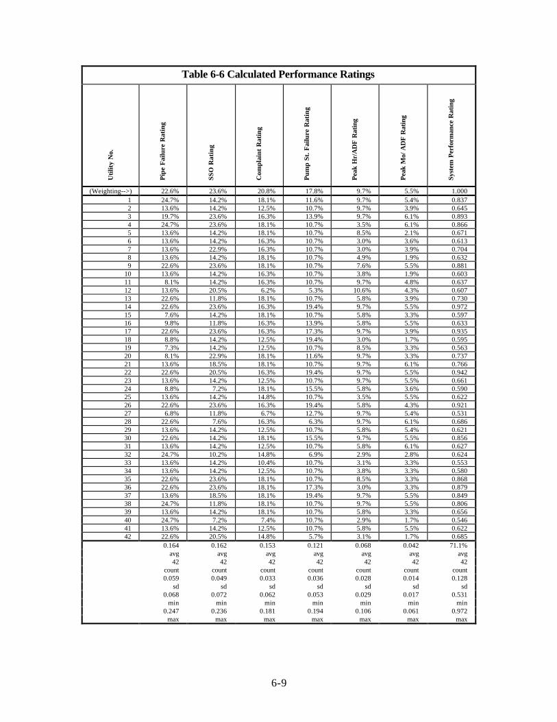
6-9

Table 6-6 Calculated Performance Ratings

Uti

lity

No.

Pip

e F

ailu

re R

atin

g

SS

O R

atin

g

Com

plai

nt R

atin

g

Pum

p St

. Fai

lure

Rat

ing

Pea

k H

r/A

DF

Rat

ing

Pea

k M

o/ A

DF

Rat

ing

Syst

em P

erfo

rman

ce R

atin

g

(Weighting-->) 22.6% 23.6% 20.8% 17.8% 9.7% 5.5% 1.0001 24.7% 14.2% 18.1% 11.6% 9.7% 5.4% 0.8372 13.6% 14.2% 12.5% 10.7% 9.7% 3.9% 0.6453 19.7% 23.6% 16.3% 13.9% 9.7% 6.1% 0.8934 24.7% 23.6% 18.1% 10.7% 3.5% 6.1% 0.8665 13.6% 14.2% 18.1% 10.7% 8.5% 2.1% 0.6716 13.6% 14.2% 16.3% 10.7% 3.0% 3.6% 0.6137 13.6% 22.9% 16.3% 10.7% 3.0% 3.9% 0.7048 13.6% 14.2% 18.1% 10.7% 4.9% 1.9% 0.6329 22.6% 23.6% 18.1% 10.7% 7.6% 5.5% 0.881

10 13.6% 14.2% 16.3% 10.7% 3.8% 1.9% 0.60311 8.1% 14.2% 16.3% 10.7% 9.7% 4.8% 0.63712 13.6% 20.5% 6.2% 5.3% 10.6% 4.3% 0.60713 22.6% 11.8% 18.1% 10.7% 5.8% 3.9% 0.73014 22.6% 23.6% 16.3% 19.4% 9.7% 5.5% 0.97215 7.6% 14.2% 18.1% 10.7% 5.8% 3.3% 0.59716 9.8% 11.8% 16.3% 13.9% 5.8% 5.5% 0.63317 22.6% 23.6% 16.3% 17.3% 9.7% 3.9% 0.93518 8.8% 14.2% 12.5% 19.4% 3.0% 1.7% 0.59519 7.3% 14.2% 12.5% 10.7% 8.5% 3.3% 0.56320 8.1% 22.9% 18.1% 11.6% 9.7% 3.3% 0.73721 13.6% 18.5% 18.1% 10.7% 9.7% 6.1% 0.76622 22.6% 20.5% 16.3% 19.4% 9.7% 5.5% 0.94223 13.6% 14.2% 12.5% 10.7% 9.7% 5.5% 0.66124 8.8% 7.2% 18.1% 15.5% 5.8% 3.6% 0.59025 13.6% 14.2% 14.8% 10.7% 3.5% 5.5% 0.62226 22.6% 23.6% 16.3% 19.4% 5.8% 4.3% 0.92127 6.8% 11.8% 6.7% 12.7% 9.7% 5.4% 0.53128 22.6% 7.6% 16.3% 6.3% 9.7% 6.1% 0.68629 13.6% 14.2% 12.5% 10.7% 5.8% 5.4% 0.62130 22.6% 14.2% 18.1% 15.5% 9.7% 5.5% 0.85631 13.6% 14.2% 12.5% 10.7% 5.8% 6.1% 0.62732 24.7% 10.2% 14.8% 6.9% 2.9% 2.8% 0.62433 13.6% 14.2% 10.4% 10.7% 3.1% 3.3% 0.55334 13.6% 14.2% 12.5% 10.7% 3.8% 3.3% 0.58035 22.6% 23.6% 18.1% 10.7% 8.5% 3.3% 0.86836 22.6% 23.6% 18.1% 17.3% 3.0% 3.3% 0.87937 13.6% 18.5% 18.1% 19.4% 9.7% 5.5% 0.84938 24.7% 11.8% 18.1% 10.7% 9.7% 5.5% 0.80639 13.6% 14.2% 18.1% 10.7% 5.8% 3.3% 0.65640 24.7% 7.2% 7.4% 10.7% 2.9% 1.7% 0.54641 13.6% 14.2% 12.5% 10.7% 5.8% 5.5% 0.62242 22.6% 20.5% 14.8% 5.7% 3.1% 1.7% 0.685

0.164 0.162 0.153 0.121 0.068 0.042 71.1%avg avg avg avg avg avg avg42 42 42 42 42 42 42

count count count count count count count0.059 0.049 0.033 0.036 0.028 0.014 0.128

sd sd sd sd sd sd sd0.068 0.072 0.062 0.053 0.029 0.017 0.531

min min min min min min min0.247 0.236 0.181 0.194 0.106 0.061 0.972

max max max max max max max

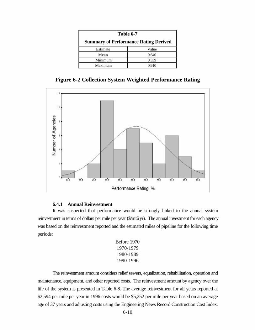
6-10

Table 6-7

Summary of Performance Rating Derived

Estimate Value

Mean 0.640Minimum 0.339Maximum 0.910

Figure 6-2 Collection System Weighted Performance Rating

6.4.1 Annual ReinvestmentIt was suspected that performance would be strongly linked to the annual system

reinvestment in terms of dollars per mile per year ($/mi$yr). The annual investment for each agency

was based on the reinvestment reported and the estimated miles of pipeline for the following time

periods:

Before 19701970-19791980-19891990-1996

The reinvestment amount considers relief sewers, equalization, rehabilitation, operation and

maintenance, equipment, and other reported costs. The reinvestment amount by agency over the

life of the system is presented in Table 6-8. The average reinvestment for all years reported at

$2,594 per mile per year in 1996 costs would be $5,252 per mile per year based on an average

age of 37 years and adjusting costs using the Engineering News Record Construction Cost Index.

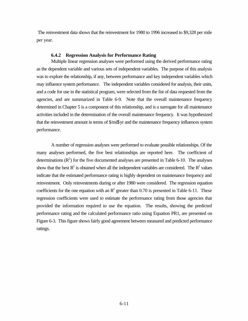
6-11

The reinvestment data shows that the reinvestment for 1980 to 1996 increased to $9,328 per mile

per year.

6.4.2 Regression Analysis for Performance RatingMultiple linear regression analyses were performed using the derived performance rating

as the dependent variable and various sets of independent variables. The purpose of this analysis

was to explore the relationship, if any, between performance and key independent variables which

may influence system performance. The independent variables considered for analysis, their units,

and a code for use in the statistical program, were selected from the list of data requested from the

agencies, and are summarized in Table 6-9. Note that the overall maintenance frequency

determined in Chapter 5 is a component of this relationship, and is a surrogate for all maintenance

activities included in the determination of the overall maintenance frequency. It was hypothesized

that the reinvestment amount in terms of $/mi$yr and the maintenance frequency influences system

performance.

A number of regression analyses were performed to evaluate possible relationships. Of the

many analyses performed, the five best relationships are reported here. The coefficient of

determinations (R2) for the five documented analyses are presented in Table 6-10. The analyses

show that the best R2 is obtained when all the independent variables are considered. The R2 values

indicate that the estimated performance rating is highly dependent on maintenance frequency and

reinvestment. Only reinvestments during or after 1980 were considered. The regression equation

coefficients for the one equation with an R2 greater than 0.70 is presented in Table 6-11. These

regression coefficients were used to estimate the performance rating from those agencies that

provided the information required to use the equation. The results, showing the predicted

performance rating and the calculated performance ratio using Equation PR1, are presented on

Figure 6-3. This figure shows fairly good agreement between measured and predicted performance

ratings.

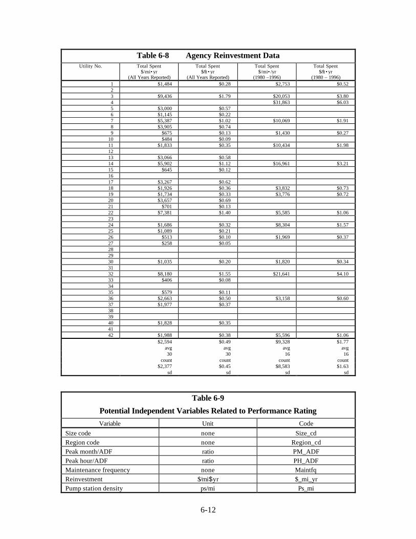
6-12

Table 6-8 Agency Reinvestment DataUtility No. Total Spent

$/mi•yr(All Years Reported)

Total Spent$/ft •yr

(All Years Reported)

Total Spent$/mi•/yr

(1980 –1996)

Total Spent$/ft •yr

(1980 – 1996)1 $1,484 $0.28 $2,753 $0.5223 $9,436 $1.79 $20,053 $3.804 $31,863 $6.035 $3,000 $0.576 $1,145 $0.227 $5,387 $1.02 $10,069 $1.918 $3,905 $0.749 $675 $0.13 $1,430 $0.27

10 $484 $0.0911 $1,833 $0.35 $10,434 $1.981213 $3,066 $0.5814 $5,902 $1.12 $16,961 $3.2115 $645 $0.121617 $3,267 $0.6218 $1,926 $0.36 $3,832 $0.7319 $1,734 $0.33 $3,776 $0.7220 $3,657 $0.6921 $701 $0.1322 $7,381 $1.40 $5,585 $1.062324 $1,686 $0.32 $8,304 $1.5725 $1,089 $0.2126 $513 $0.10 $1,969 $0.3727 $258 $0.05282930 $1,035 $0.20 $1,820 $0.343132 $8,180 $1.55 $21,641 $4.1033 $406 $0.083435 $579 $0.1136 $2,663 $0.50 $3,158 $0.6037 $1,977 $0.37383940 $1,828 $0.354142 $1,988 $0.38 $5,596 $1.06

$2,594 $0.49 $9,328 $1.77avg avg avg avg30 30 16 16

count count count count$2,377 $0.45 $8,583 $1.63

sd sd sd sd

Table 6-9

Potential Independent Variables Related to Performance Rating

Variable Unit Code

Size code none Size_cd

Region code none Region_cd

Peak month/ADF ratio PM_ADF

Peak hour/ADF ratio PH_ADF

Maintenance frequency none Maintfq

Reinvestment $/mi$yr $_mi_yr

Pump station density ps/mi Ps_mi

6-13

Table 6-10

Regression Analysis for Performance Ratios

Independent Variables Coefficient ofDetermination

Selected RegressionAnalysis

Rei

nves

tmen

t, $/

mi$

yr

Reg

iona

l Cod

e

Siz

e C

ode

Pea

k M

onth

/AD

F

Pea

k H

our/

AD

F

Pum

p S

tati

ons/

Mi

Mai

nten

ance

Fre

quen

cy

R2Adjusted

R2 R2 > 0.70

Equation Name

X X X 0.34380 0.11820

X X X X 0.35678 0.12730

X X X X X 0.57434 0.32987

X X X X X X 0.71141 0.50611

X X X X X X X 0.84710 0.71757 X PR1

Table 6-11Regression Coefficients for

Performance RatingItem Line Regression Equation Coefficients

Eq PR1 Bi

Constant 0.751

$/mi$yr 3.342 x 10-6

Regional Code 2.179 x 10-2

Size Code -1.114 x 10-2

Peak Month/ADF -0.117

Peak Hour/ADF -1.487 x 10-2

Pump Stations/mi -0.252

Maintenance Frequency 2.614

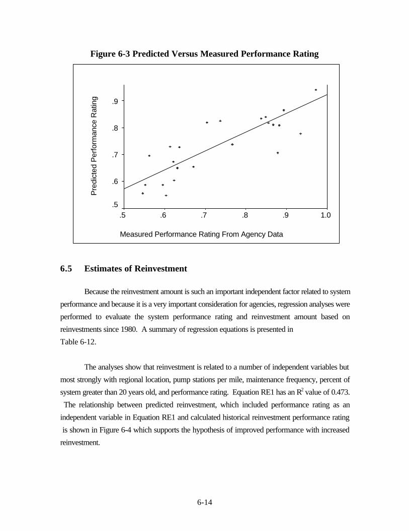
6-14

Figure 6-3 Predicted Versus Measured Performance Rating

6.5 Estimates of Reinvestment

Because the reinvestment amount is such an important independent factor related to system

performance and because it is a very important consideration for agencies, regression analyses were

performed to evaluate the system performance rating and reinvestment amount based on

reinvestments since 1980. A summary of regression equations is presented in

Table 6-12.

The analyses show that reinvestment is related to a number of independent variables but

most strongly with regional location, pump stations per mile, maintenance frequency, percent of

system greater than 20 years old, and performance rating. Equation RE1 has an R2 value of 0.473.

The relationship between predicted reinvestment, which included performance rating as an

independent variable in Equation RE1 and calculated historical reinvestment performance rating

is shown in Figure 6-4 which supports the hypothesis of improved performance with increased

reinvestment.

Measured Performance Rating From Agency Data

1.0.9.8.7.6.5

Pre

dict

ed P

erfo

rman

ce R

atin

g .9

.8

.7

.6

.5

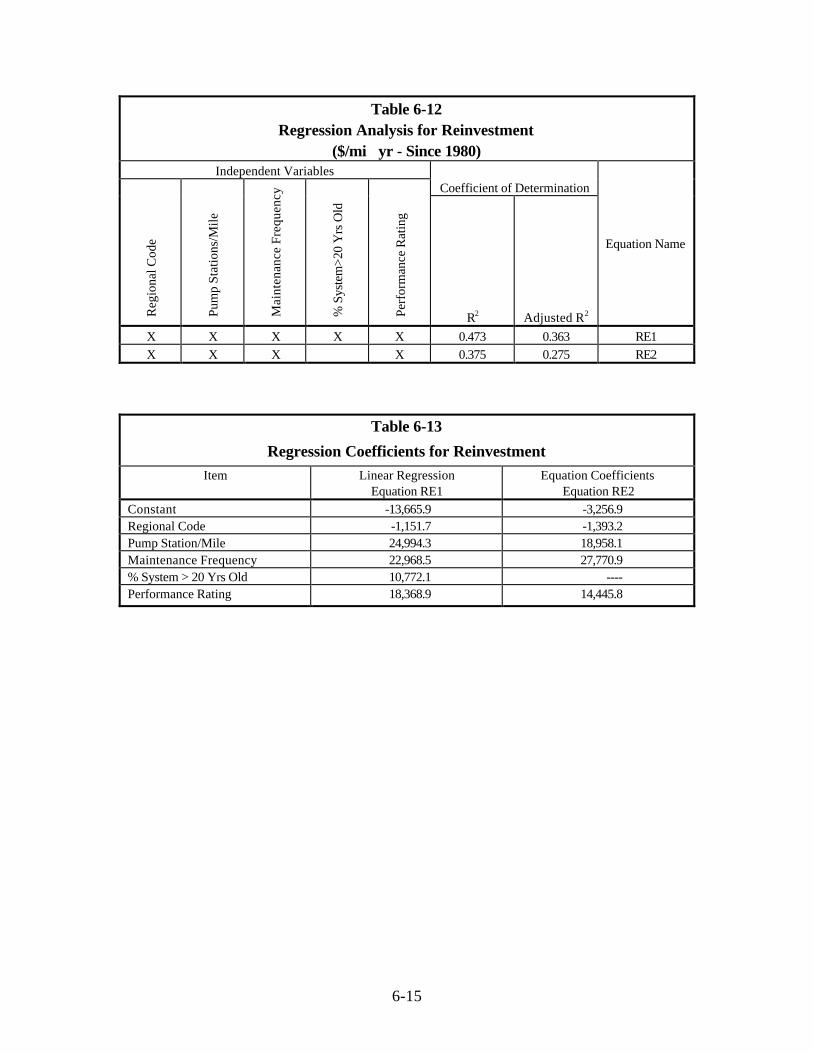
6-15

Table 6-12Regression Analysis for Reinvestment

($/mi�yr - Since 1980)Independent Variables

Coefficient of Determination

Reg

iona

l Cod

e

Pum

p S

tati

ons/

Mil

e

Mai

nten

ance

Fre

quen

cy

% S

yste

m>

20 Y

rs O

ld

Per

form

ance

Rat

ing

R2 Adjusted R2

Equation Name

X X X X X 0.473 0.363 RE1

X X X X 0.375 0.275 RE2

Table 6-13

Regression Coefficients for Reinvestment

Item Linear RegressionEquation RE1

Equation CoefficientsEquation RE2

Constant -13,665.9 -3,256.9Regional Code -1,151.7 -1,393.2Pump Station/Mile 24,994.3 18,958.1Maintenance Frequency 22,968.5 27,770.9% System > 20 Yrs Old 10,772.1 ----Performance Rating 18,368.9 14,445.8

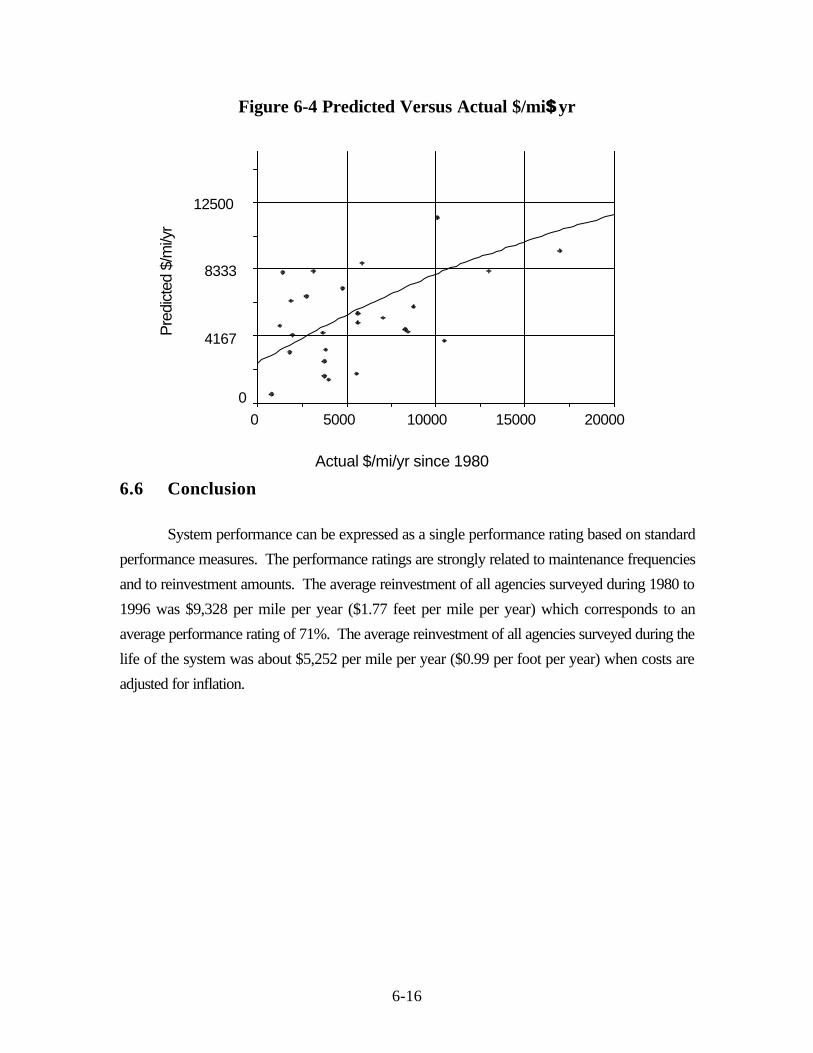
6-16

Figure 6-4 Predicted Versus Actual $/mi$$yr

6.6 Conclusion

System performance can be expressed as a single performance rating based on standard

performance measures. The performance ratings are strongly related to maintenance frequencies

and to reinvestment amounts. The average reinvestment of all agencies surveyed during 1980 to

1996 was $9,328 per mile per year ($1.77 feet per mile per year) which corresponds to an

average performance rating of 71%. The average reinvestment of all agencies surveyed during the

life of the system was about $5,252 per mile per year ($0.99 per foot per year) when costs are

adjusted for inflation.

Actual $/mi/yr since 1980

20000150001000050000

Pre

dict

ed $

/mi/y

r

12500

8333

4167

0

7-1

7.0 Optimizing Collection System Maintenance

7.1 Introduction

This chapter presents maintenance frequencies, performance ratings, and reinvestment rates

for optimizing collection system maintenance activities. Optimization should provide a system which

performs satisfactorily with a reasonable level of maintenance (reinvestment). It should be

remembered that each collection system has its own unique characteristics and requirements and

that the information presented in this study is intended to provide guidance for improving system

performance through a more balanced maintenance program and appropriate levels of reinvestment.

The guidelines presented herein relative to system performance, maintenance levels, and

reinvestment will help agencies determine how much maintenance is enough. In order to optimize

collection system maintenance, it is necessary to establish the existing system maintenance

frequency, performance rating, and reinvestment rate as discussed in the following sections.

7.2 Collection System Maintenance Frequency

The following sections present the methods to determine the maintenance frequency of a

given system.

7.2.1 Establish Existing Maintenance Frequency

All maintenance activities should be expressed as rates, such as percentage of system

cleaned per year. The procedure presented in Chapter 5 can be used to develop the overall

maintenance frequency. The maintenance activities listed in Table 7-1 should be considered when

developing the system maintenance frequency.

7-2

Table 7-1

Activities for Determination of Maintenance Frequencies

Maintenance Activity Suggested Rate Expression

Cleaning of sewer lines Percentage of system/yr

Root removal Percentage of system/yr

Pump Station Inspections number/pump station$yr

Flow monitoring Percentage of system/yr

Manhole inspection Percentage of system/yr

Smoke/dye testing Percentage of system/yr

CCTV Percentage of system/yr

Private sector Inspections Percentage of system/yr

Manholes rehabilitated Percentage of manholes requiring rehabilitation actually rehabilitated

Sewer line rehabilitated Percentage of sewer lines requiring rehabilitation actually rehabilitated

Relief/equalization Percentage of relief/equalization facilities needed actually constructed

Private sectors rehabilitated Percentage of private sector needs actually addressed

The following steps describe the determination of system maintenance frequency:

(1) Determine Maintenance Activity Rate

For each maintenance activity, a rate is calculated. For most routine maintenance activities,

such as line cleaning, the maintenance activity rate is expressed as the percentage of system cleaned

per unit time (%/yr). For example, an agency which has 1,500 miles of sewer and has cleaned 825

miles of sewers over a 5-year period, has a cleaning maintenance rate of 11%/yr determined as

follows:

825 miles / (5 years x 1500 miles) = 0.11 = 11% per year

(2) Assign Normalized Frequency to Each Maintenance Activity

Using the data presented in Chapter 5, a normalized frequency rate is assigned to each

maintenance activity. This allows the overall maintenance frequency to be determined considering

multiple maintenance activities. The normalized frequency for each maintenance activity and the

activity rate from Chapter 5 are summarized in Table 7-2. For example, an agency which has a line

cleaning frequency of 11%/yr (0.11) will have a normalized maintenance frequency of 5% for this

activity.

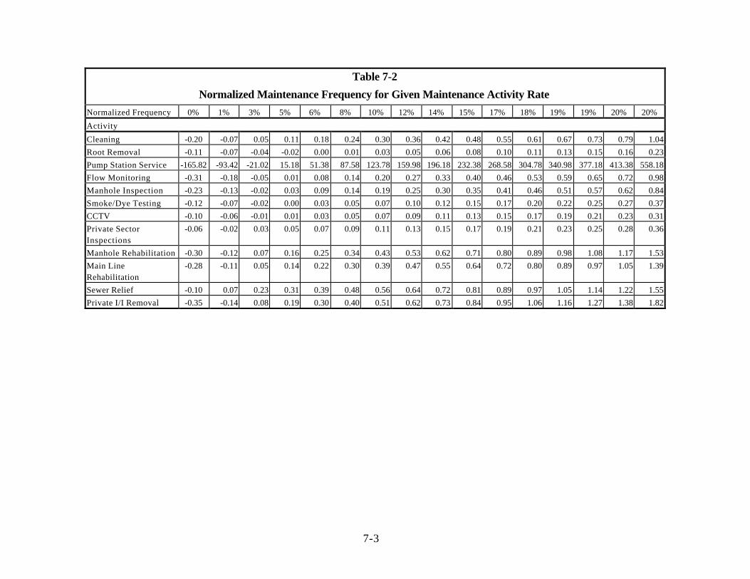
7-3

Table 7-2

Normalized Maintenance Frequency for Given Maintenance Activity Rate

Normalized Frequency 0% 1% 3% 5% 6% 8% 10% 12% 14% 15% 17% 18% 19% 19% 20% 20%

Activity

Cleaning -0.20 -0.07 0.05 0.11 0.18 0.24 0.30 0.36 0.42 0.48 0.55 0.61 0.67 0.73 0.79 1.04

Root Removal -0.11 -0.07 -0.04 -0.02 0.00 0.01 0.03 0.05 0.06 0.08 0.10 0.11 0.13 0.15 0.16 0.23

Pump Station Service -165.82 -93.42 -21.02 15.18 51.38 87.58 123.78 159.98 196.18 232.38 268.58 304.78 340.98 377.18 413.38 558.18

Flow Monitoring -0.31 -0.18 -0.05 0.01 0.08 0.14 0.20 0.27 0.33 0.40 0.46 0.53 0.59 0.65 0.72 0.98

Manhole Inspection -0.23 -0.13 -0.02 0.03 0.09 0.14 0.19 0.25 0.30 0.35 0.41 0.46 0.51 0.57 0.62 0.84

Smoke/Dye Testing -0.12 -0.07 -0.02 0.00 0.03 0.05 0.07 0.10 0.12 0.15 0.17 0.20 0.22 0.25 0.27 0.37

CCTV -0.10 -0.06 -0.01 0.01 0.03 0.05 0.07 0.09 0.11 0.13 0.15 0.17 0.19 0.21 0.23 0.31

Private SectorInspections

-0.06 -0.02 0.03 0.05 0.07 0.09 0.11 0.13 0.15 0.17 0.19 0.21 0.23 0.25 0.28 0.36

Manhole Rehabilitation -0.30 -0.12 0.07 0.16 0.25 0.34 0.43 0.53 0.62 0.71 0.80 0.89 0.98 1.08 1.17 1.53

Main LineRehabilitation

-0.28 -0.11 0.05 0.14 0.22 0.30 0.39 0.47 0.55 0.64 0.72 0.80 0.89 0.97 1.05 1.39

Sewer Relief -0.10 0.07 0.23 0.31 0.39 0.48 0.56 0.64 0.72 0.81 0.89 0.97 1.05 1.14 1.22 1.55

Private I/I Removal -0.35 -0.14 0.08 0.19 0.30 0.40 0.51 0.62 0.73 0.84 0.95 1.06 1.16 1.27 1.38 1.82

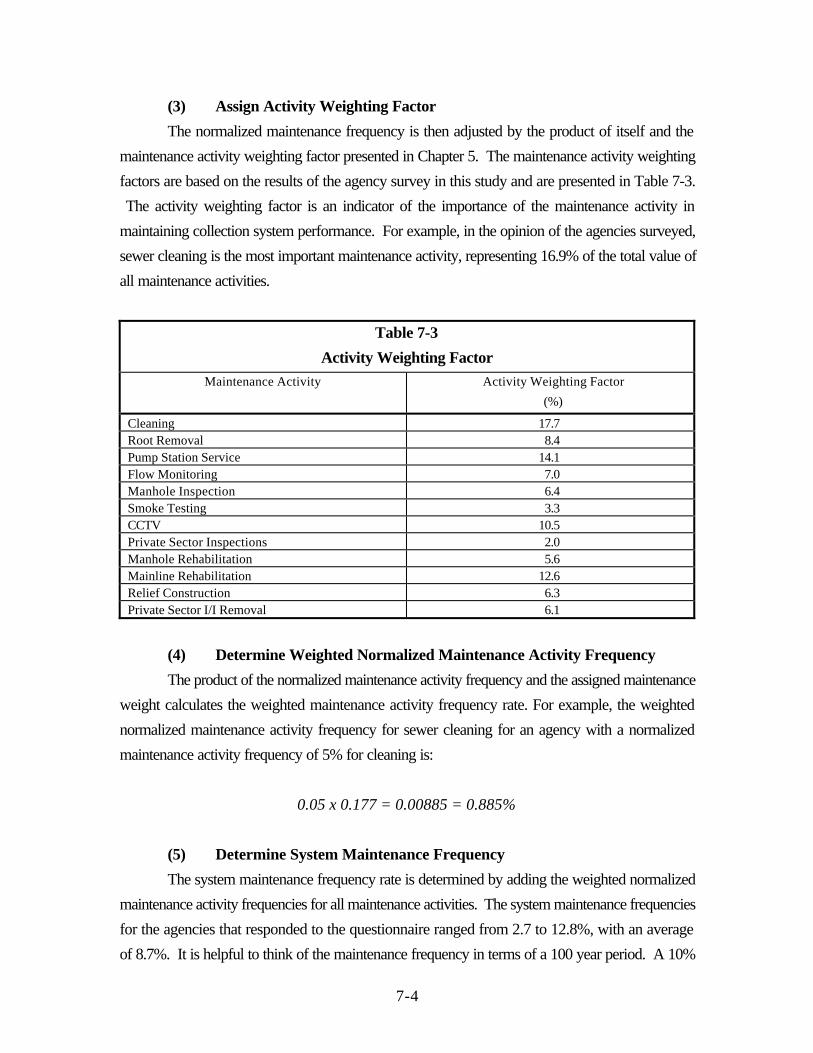
7-4

(3) Assign Activity Weighting Factor

The normalized maintenance frequency is then adjusted by the product of itself and the

maintenance activity weighting factor presented in Chapter 5. The maintenance activity weighting

factors are based on the results of the agency survey in this study and are presented in Table 7-3.

The activity weighting factor is an indicator of the importance of the maintenance activity in

maintaining collection system performance. For example, in the opinion of the agencies surveyed,

sewer cleaning is the most important maintenance activity, representing 16.9% of the total value of

all maintenance activities.

Table 7-3

Activity Weighting Factor

Maintenance Activity Activity Weighting Factor

(%)

Cleaning 17.7Root Removal 8.4Pump Station Service 14.1Flow Monitoring 7.0Manhole Inspection 6.4Smoke Testing 3.3CCTV 10.5Private Sector Inspections 2.0Manhole Rehabilitation 5.6Mainline Rehabilitation 12.6Relief Construction 6.3Private Sector I/I Removal 6.1

(4) Determine Weighted Normalized Maintenance Activity Frequency

The product of the normalized maintenance activity frequency and the assigned maintenance

weight calculates the weighted maintenance activity frequency rate. For example, the weighted

normalized maintenance activity frequency for sewer cleaning for an agency with a normalized

maintenance activity frequency of 5% for cleaning is:

0.05 x 0.177 = 0.00885 = 0.885%

(5) Determine System Maintenance Frequency

The system maintenance frequency rate is determined by adding the weighted normalized

maintenance activity frequencies for all maintenance activities. The system maintenance frequencies

for the agencies that responded to the questionnaire ranged from 2.7 to 12.8%, with an average

of 8.7%. It is helpful to think of the maintenance frequency in terms of a 100 year period. A 10%

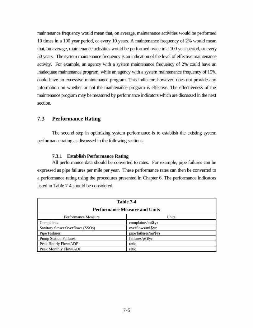
7-5

maintenance frequency would mean that, on average, maintenance activities would be performed

10 times in a 100 year period, or every 10 years. A maintenance frequency of 2% would mean

that, on average, maintenance activities would be performed twice in a 100 year period, or every

50 years. The system maintenance frequency is an indication of the level of effective maintenance

activity. For example, an agency with a system maintenance frequency of 2% could have an

inadequate maintenance program, while an agency with a system maintenance frequency of 15%

could have an excessive maintenance program. This indicator, however, does not provide any

information on whether or not the maintenance program is effective. The effectiveness of the

maintenance program may be measured by performance indicators which are discussed in the next

section.

7.3 Performance Rating

The second step in optimizing system performance is to establish the existing system

performance rating as discussed in the following sections.

7.3.1 Establish Performance RatingAll performance data should be converted to rates. For example, pipe failures can be

expressed as pipe failures per mile per year. These performance rates can then be converted to

a performance rating using the procedures presented in Chapter 6. The performance indicators

listed in Table 7-4 should be considered.

Table 7-4

Performance Measure and Units

Performance Measure Units

Complaints complaints/mi$yrSanitary Sewer Overflows (SSOs) overflows/mi$yrPipe Failures pipe failures/mi$yrPump Station Failures failures/ps$yrPeak Hourly Flow/ADF ratioPeak Monthly Flow/ADF ratio

7-6

The following steps should be taken to calculate the performance rating:

(1) Determine Performance Measure Rate

For each performance measure, a performance rate is calculated. The performance rate

in most cases is defined as the number of occurrences divided by the number of years for which the

performance indicator is reported and by the total miles of sewer in the system. For example, the

pipe failure performance rate for an agency which has 1,500 miles of sewer and has experienced

370 pipe failures over a 5-year period can be calculated as follows:

370 pipe failures / (5 years x 1500 miles) = 0.049 failures/mi$year

The performance rate for pump station failures is calculated by dividing the number of pump

station failures per year by the number of pump stations. The flow performance indicators, peak

hour and peak month to average daily flow are expressed as a ratio.

(2) Assign Normalized Performance Rating to Each Performance Measure

Using the data presented in Chapter 6, a normalized performance rating is assigned to each

performance measurement. The normalized performance rating for each performance measure is

presented in Table 7-5. For example, an agency which has a performance measure of 0.049

failures/mi$yr for pipe failure, will have a normalized performance rating of 50% for this item.

(3) Assign Performance Weighting Factor

The normalized performance rating is then adjusted by multiplying it by the activity

weighting factor presented in Chapter 6. The performance activity weighting factors for each

performance measure are presented in Table 7-6. The performance weighing factor is a measure

of the importance of the performance measure as perceived by the agencies that participated in this

survey. For example, the largest weighting factor of 23.6% was assigned to SSO=s.

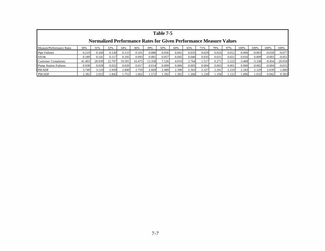
7-7

Table 7-5

Normalized Performance Rates for Given Performance Measure ValuesMeasure/Performance Rates 30% 31% 32% 34% 36% 39% 50% 60% 65% 71% 79% 97% 100% 100% 100% 100%

Pipe Failures 0.219 0.160 0.130 0.115 0.101 0.086 0.056 0.041 0.035 0.029 0.024 0.012 0.006 -0.003 -0.018 -0.077

SSO=s 0.189 0.141 0.117 0.105 0.093 0.081 0.057 0.045 0.040 0.035 0.031 0.021 0.016 0.009 -0.003 -0.051

Customer Complaints 41.403 28.939 22.707 19.591 16.475 13.358 7.126 4.010 2.764 1.517 0.271 -2.222 -3.468 -5.338 -8.454 -20.918

Pump Station Failures 0.038 0.028 0.022 0.020 0.017 0.014 0.009 0.006 0.005 0.004 0.003 0.001 0.000 -0.002 -0.004 -0.015

PH/ADF 3.749 3.119 2.939 2.849 2.759 2.669 2.489 2.399 2.363 2.327 2.291 2.219 2.183 2.129 2.039 1.000

PM/ADF 2.382 2.022 1.842 1.752 1.662 1.572 1.392 1.302 1.266 1.230 1.194 1.122 1.086 1.032 0.942 0.583

7-8

Table 7-6Performance Weighting Factor

Performance Measure Weighting Factor(%)

Customer Complaints 22.6

Sanitary Sewer Overflows (SSO=s) 23.6

Pipe Failures 20.8

Pump Station Failures 17.8

Peak Hourly/ADF Ratio 9.7

Peak Monthly/ADF Ratio 5.5

(4) Calculate Weighted Normalized Performance Rating

The weighted normalized performance rating is calculated by the product of the weighting

factor and the normalized performance rate. For example, the weighted normalized performance

rating of pipe failure for an agency with a normalized performance rating of 50% is:

0.50 x 0.208=0.104 = 10.4%

(5) Determine Overall System Performance Rating

The overall system performance rating is calculated by summing the weighted normalized

performance ratings of the six performance measures. The weighted performance rating for the

agencies that responded to the questionnaire varied from 33.9 to 91.0%, with an average of 64%.

The performance rating is an indication of the level of system performance. For example, an agency

with a performance rating of 30% probably is not providing effective service to its customers while

an agency with a performance rating of 80% is likely providing safe and effective service.

7.4 Determine Historical Reinvestment Rate

The historical reinvestment rate should be determined based on the information in Table 7-

7. If cost data for the life of the system is not available, then the longest period for which data is

available should be used. Only costs related to the collection system should be included. The costs

of facilities such as wastewater treatment plants should not be included. The reinvestment rate will

provide a basis for comparison with other agencies regarding the adequacy of the budget for system

maintenance, and can also be compared with predicted reinvestment amounts which may be

estimated from system operating characteristics as discussed in this section.

Table 7-7

Determination of Reinvestment

Reinvestment Item Unit

Relief construction $/mi$yr, over the life of the system

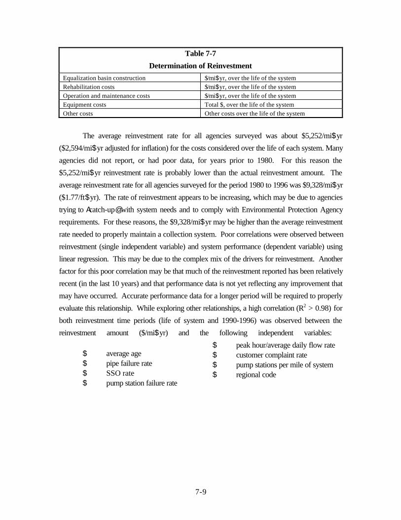
7-9

Table 7-7


Equalization basin construction $/mi$yr, over the life of the system

Rehabilitation costs $/mi$yr, over the life of the system

Operation and maintenance costs $/mi$yr, over the life of the system

Equipment costs Total $, over the life of the system

Other costs Other costs over the life of the system

The average reinvestment rate for all agencies surveyed was about $5,252/mi$yr

($2,594/mi$yr adjusted for inflation) for the costs considered over the life of each system. Many

agencies did not report, or had poor data, for years prior to 1980. For this reason the

$5,252/mi$yr reinvestment rate is probably lower than the actual reinvestment amount. The

average reinvestment rate for all agencies surveyed for the period 1980 to 1996 was $9,328/mi$yr

($1.77/ft$yr). The rate of reinvestment appears to be increasing, which may be due to agencies

trying to Acatch-up@ with system needs and to comply with Environmental Protection Agency

requirements. For these reasons, the $9,328/mi$yr may be higher than the average reinvestment

rate needed to properly maintain a collection system. Poor correlations were observed between

reinvestment (single independent variable) and system performance (dependent variable) using

linear regression. This may be due to the complex mix of the drivers for reinvestment. Another

factor for this poor correlation may be that much of the reinvestment reported has been relatively

recent (in the last 10 years) and that performance data is not yet reflecting any improvement that

may have occurred. Accurate performance data for a longer period will be required to properly

evaluate this relationship. While exploring other relationships, a high correlation (R2 > 0.98) for

both reinvestment time periods (life of system and 1990-1996) was observed between the

reinvestment amount ($/mi$yr) and the following independent variables:

$ average age$ pipe failure rate$ SSO rate$ pump station failure rate

$ peak hour/average daily flow rate$ customer complaint rate$ pump stations per mile of system$ regional code

7-10

The regression coefficients for the reinvestment rates based on survey data are presented

in Table 7-8.

Table 7-8Reinvestment Regression Coefficients

Dependent Variable: $/mi$yr Reinvestment

Independent VariableEquation RE-3

Based on All Reinvestment DataEquation RE-4

Based on 1980 to 1996 Data

Customer Complaint Rate(1) -2836.49 -6114.06

SSO=s (1) -63550.25 -101100.93

Pipe Failure Rate(1) -42308.86 -19817.16

Pump Station Failure Rate(1) -131572.22 -251085.23

Regional Code -56.04 -942.45

Pump Stations Per Mile 17055.97 46788.79

Peak Hour/ADF Ratio -3616.08 -6915.00

Average Age 191.08 642.09

Constant 13288.45 17776.14

R2 0.998 0.984

Adjusted R2 0.980 0.860(1) Five years of data ending 1996.

It must be remembered that the sample used for this study is relatively small and that some

of the agencies likely have very good maintenance programs while the programs of others are

deficient. If all agencies had optimized maintenance activities and high quality data, a stronger

correlation between reinvestment and performance would be expected. Nevertheless, the

reinvestment trends provide some insight into the adequacy of the total reinvestment. In order to

develop a better perspective of the relationship between performance and reinvestment, an

estimated performance/reinvestment envelope was constructed using the average performance

ratios and the reinvestment rates previously presented. For a performance rating of 0.65 to 0.80

cost ranges of $2,500/mi$yr to $8,000/mi$yr and $3,000/mi$yr to $9,700/mi$yr, respectively,

appear to form a reasonable envelope of values. The estimated envelope showing reinvestment and

desired performance is shown on Figure 7-1. Based on data from the agencies surveyed it was

assumed that a desirable range of system performance would be from about 0.65 to 0.80. The

data show that a moderate reinvestment level of $5,200/mi$yr to $6,500/mi$yr would be required

to achieve this performance. Reinvestment rates higher than the moderate value may indicate that

too much money is being spent for the benefit derived, and that some program adjustment is

warranted. Reinvestment rates lower than the moderate values indicate a very effective

reinvestment program. These values are only guidelines and must be evaluated carefully for each

agency.

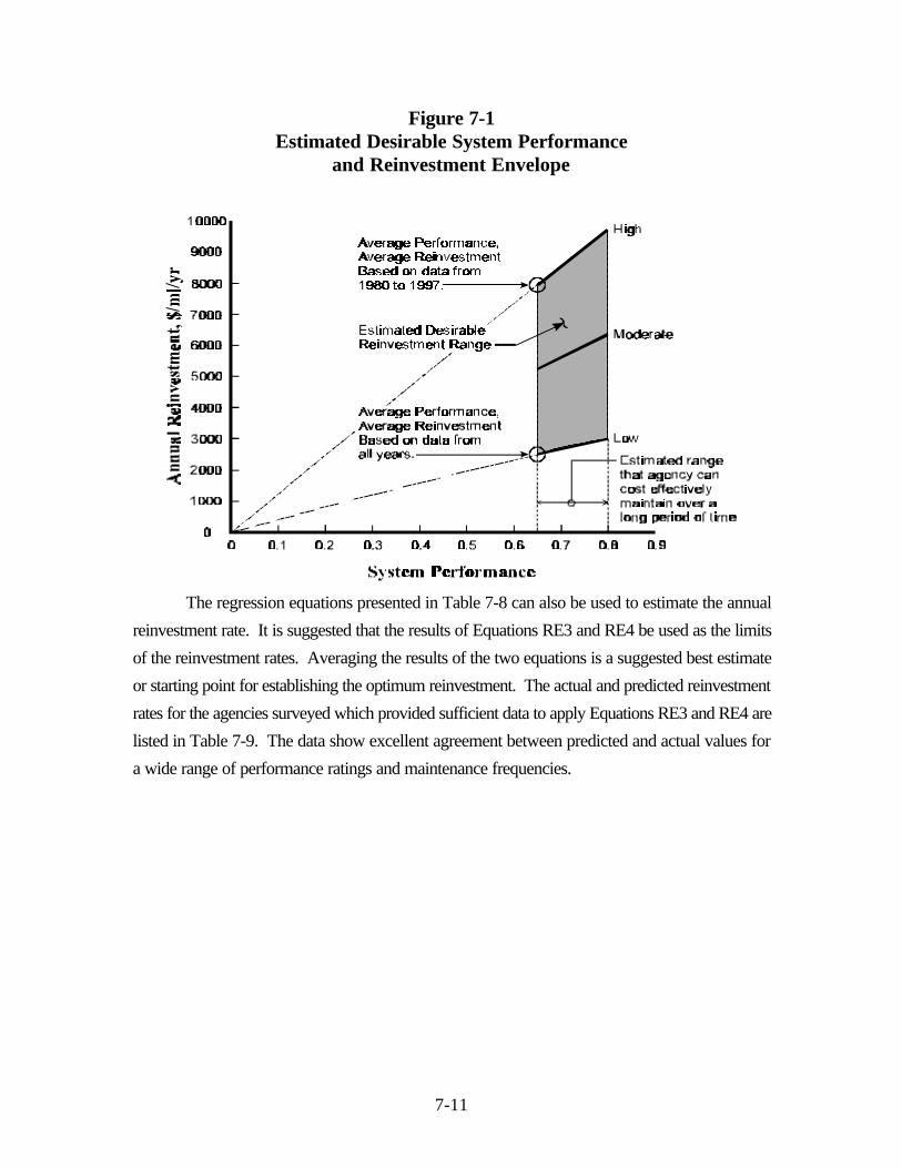
7-11

Figure 7-1Estimated Desirable System Performance

and Reinvestment Envelope

The regression equations presented in Table 7-8 can also be used to estimate the annual

reinvestment rate. It is suggested that the results of Equations RE3 and RE4 be used as the limits

of the reinvestment rates. Averaging the results of the two equations is a suggested best estimate

or starting point for establishing the optimum reinvestment. The actual and predicted reinvestment

rates for the agencies surveyed which provided sufficient data to apply Equations RE3 and RE4 are

listed in Table 7-9. The data show excellent agreement between predicted and actual values for

a wide range of performance ratings and maintenance frequencies.

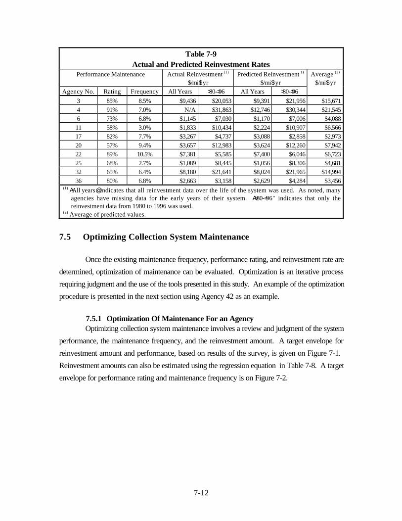
7-12

Table 7-9Actual and Predicted Reinvestment Rates

Performance Maintenance Actual Reinvestment (1)

$/mi$yrPredicted Reinvestment 1)

$/mi$yr

Agency No. Rating Frequency All Years >80-=96 All Years >80-=96

Average (2)

$/mi$yr

3 85% 8.5% $9,436 $20,053 $9,391 $21,956 $15,671

4 91% 7.0% N/A $31,863 $12,746 $30,344 $21,545

6 73% 6.8% $1,145 $7,030 $1,170 $7,006 $4,088

11 58% 3.0% $1,833 $10,434 $2,224 $10,907 $6,566

17 82% 7.7% $3,267 $4,737 $3,088 $2,858 $2,973

20 57% 9.4% $3,657 $12,983 $3,624 $12,260 $7,942

22 89% 10.5% $7,381 $5,585 $7,400 $6,046 $6,723

25 68% 2.7% $1,089 $8,445 $1,056 $8,306 $4,681

32 65% 6.4% $8,180 $21,641 $8,024 $21,965 $14,994

36 80% 6.8% $2,663 $3,158 $2,629 $4,284 $3,456

(1) AAll years@ indicates that all reinvestment data over the life of the system was used. As noted, manyagencies have missing data for the early years of their system. A>80-=96" indicates that only thereinvestment data from 1980 to 1996 was used.

(2) Average of predicted values.

7.5 Optimizing Collection System Maintenance

Once the existing maintenance frequency, performance rating, and reinvestment rate are

determined, optimization of maintenance can be evaluated. Optimization is an iterative process

requiring judgment and the use of the tools presented in this study. An example of the optimization

procedure is presented in the next section using Agency 42 as an example.

7.5.1 Optimization Of Maintenance For an AgencyOptimizing collection system maintenance involves a review and judgment of the system

performance, the maintenance frequency, and the reinvestment amount. A target envelope for

reinvestment amount and performance, based on results of the survey, is given on Figure 7-1.

Reinvestment amounts can also be estimated using the regression equation in Table 7-8. A target

envelope for performance rating and maintenance frequency is on Figure 7-2.

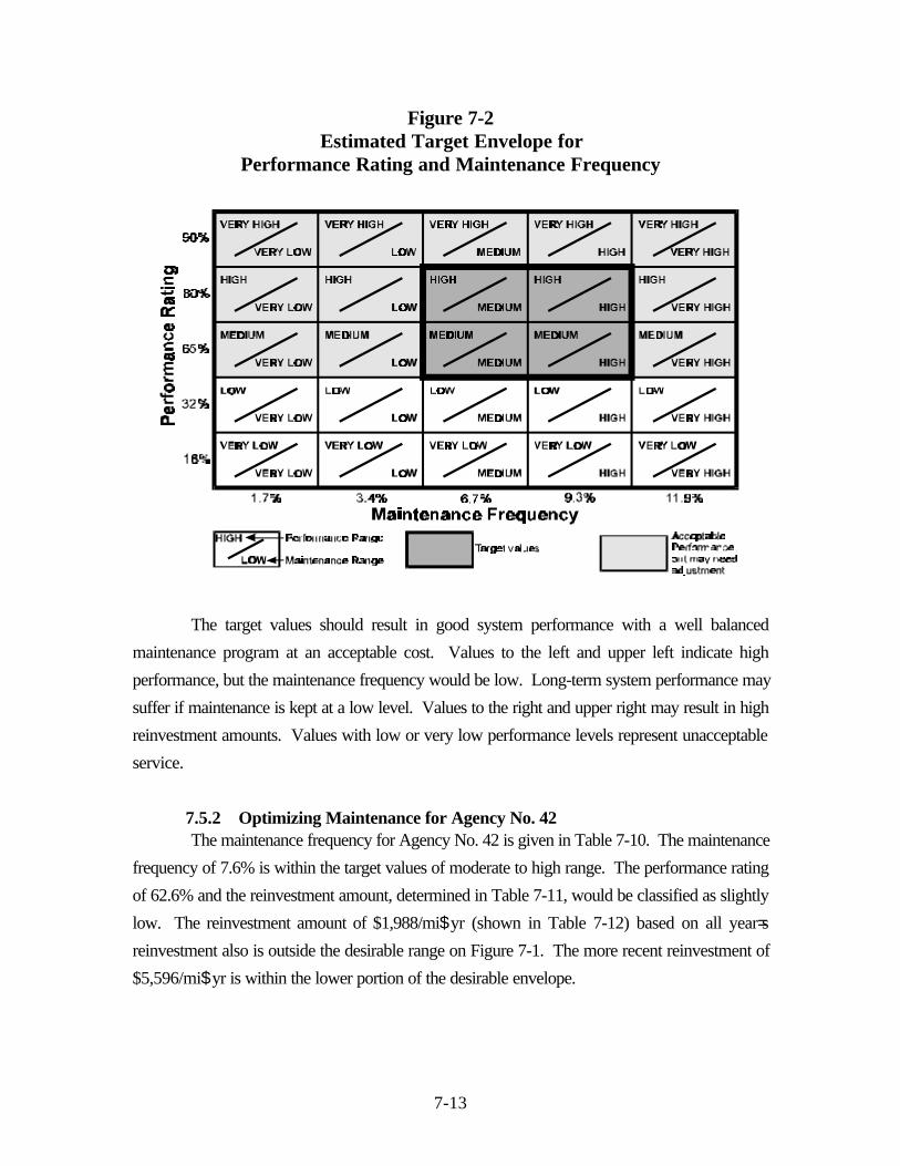
7-13

Figure 7-2Estimated Target Envelope for

Performance Rating and Maintenance Frequency

The target values should result in good system performance with a well balanced

maintenance program at an acceptable cost. Values to the left and upper left indicate high

performance, but the maintenance frequency would be low. Long-term system performance may

suffer if maintenance is kept at a low level. Values to the right and upper right may result in high

reinvestment amounts. Values with low or very low performance levels represent unacceptable

service.

7.5.2 Optimizing Maintenance for Agency No. 42The maintenance frequency for Agency No. 42 is given in Table 7-10. The maintenance

frequency of 7.6% is within the target values of moderate to high range. The performance rating

of 62.6% and the reinvestment amount, determined in Table 7-11, would be classified as slightly

low. The reinvestment amount of $1,988/mi$yr (shown in Table 7-12) based on all year=s

reinvestment also is outside the desirable range on Figure 7-1. The more recent reinvestment of

$5,596/mi$yr is within the lower portion of the desirable envelope.

7-14

Review of the individual performance measures shows that customer complaints, pump

station failures, peak hour/ADF ratio, and maximum month/ADF ratio are all below desirable

performance levels. A strategy to improve system performance would be to address maintenance

items that are most likely to improve the performance deficiencies. The number of pump station

failures could be reduced by increasing the number of inspections per year, and customer

complaints may be reduced by increasing relief sewer improvements and/or reducing flows.

Implementation of these measures will require increased reinvestment in the form of relief, and

possible adjustment of priorities and budget.

Table 7-10Determination of Maintenance Frequency for Agency No. 42

Characteristic Data: Value

Miles of Sewer - No.42 525

Number of Pump Stations 55

Data

Activity Quantity Years Rate

Cleaning 1992 -1996, miles 844 5 32.2%

Root Removal 1992 - 1996, miles 20 5 0.8%

Pump Station Inspections 1992 - 1996 1,1876 5 43.2%

Percentage of Flow Monitoring Last 5 Years 2% 5 0.4%

Percentage of Manhole Inspections Last 5 Years 100% 5 20.0%

Percentage of Smoke/Dye Test Last 5 Years 0% 5 0.0%

Percentage of CCTV Last 5 Years 5% 5 1.0%

Percentage of Private Sector Last 5 Years 0% 5 0.0%

Percentage of Manhole Rehabed 95% n/a 95.0%

Percentage of Main Line Rehabed 60% n/a 60.0%

Percentage of Relief/ Equal 0% n/a 0.0%

Percentage of Private Sector 0% n/a 0.0%

Maintenance Activity Frequency

Item Rate

Cleaning Rate, % system/year 32.2%

Root Cutting, % System/yr 0.8%

Pump Station Rate, no/ps$yr 43.2

Flow Monitoring Rate,% System/yr 0.4%

Manhole Inspect. % System/yr 20.0%

Smoke/dye Rate, % System/yr 0.0%

CCTV Rate, % System/yr 1.0%

Maintenance Activity Frequency

Item Rate

Private Sector Inspection Rate, % System/yr 0.0%

Manhole Rehab Status 95%

Main Line Rehab Status 60%

Sewer Relief Status 0%

Private I/I Removal Rating 0%

7-15

Table 7-10Determination of Maintenance Frequency for Agency No. 42

Weighted Normalized Maintenance Activity Frequency

Rating WeightUnadjustedFrequency

WeightedFrequency

Cleaning Rating 17.7% 10% 1.77%

Root Cutting Rating 8.4% 6% 0.50%

Pump Station Rating 14.1% 5% 0.71%

Flow Monitoring Rating 7.0% 3% 0.21%

Manhole Inspect Rating 6.4% 10% 0.64%

Smoke/dye Rating 3.3% 3% 0.10%

CCTV Rating 10.5% 5% 0.53%

Private Sector Inspection Rating 2.0% 1% 0.02%

Manhole Rehab Rating 5.6% 18% 1.01%

Main Line Rehab Rating 12.6% 14% 1.76%

Sewer Relief Rating 6.3% 0% 0.00%

Private I/I Removal Rating 6.1% 1% 0.06%

Total Maintenance Frequency Rating 100.0% 76.0% 7.30%

Table 7-11

Determination of Performance Rating for Agency No. 42

Data

Performance Measure Value

Pipe Failure Rate Last 5 Years, no/yr$mi 0.001

SSO Rate Last 5 Years, no/yr$mi 0.029

Customer Complaints Last 5 Years., no/mi$yr 1.552

Pump Station Failures Last 5 Years., no/mi$yr 0.023

Peak Hourly/ADF 3.000

Peak Month/ADF 2.500

Weighted Normalized Performance Activity Rating

Performance Rating WeightUnadjusted

RatingWeighted

Rating

Pipe Failure Rating 22.6% 100% 22.6%

SSO Rate Rating 23.6% 87.1% 20.5%

Customer Complaints Rating 20.8% 71.3% 14.8%

Pump Station Failures Rating 17.8% 32.1% 5.7%

Peak Hourly/ADF Rating 9.7% 32.1% 3.1%

Peak Month/ADF Rating 5.5% 30.0% 1.7%

Total 100% 68.5 %

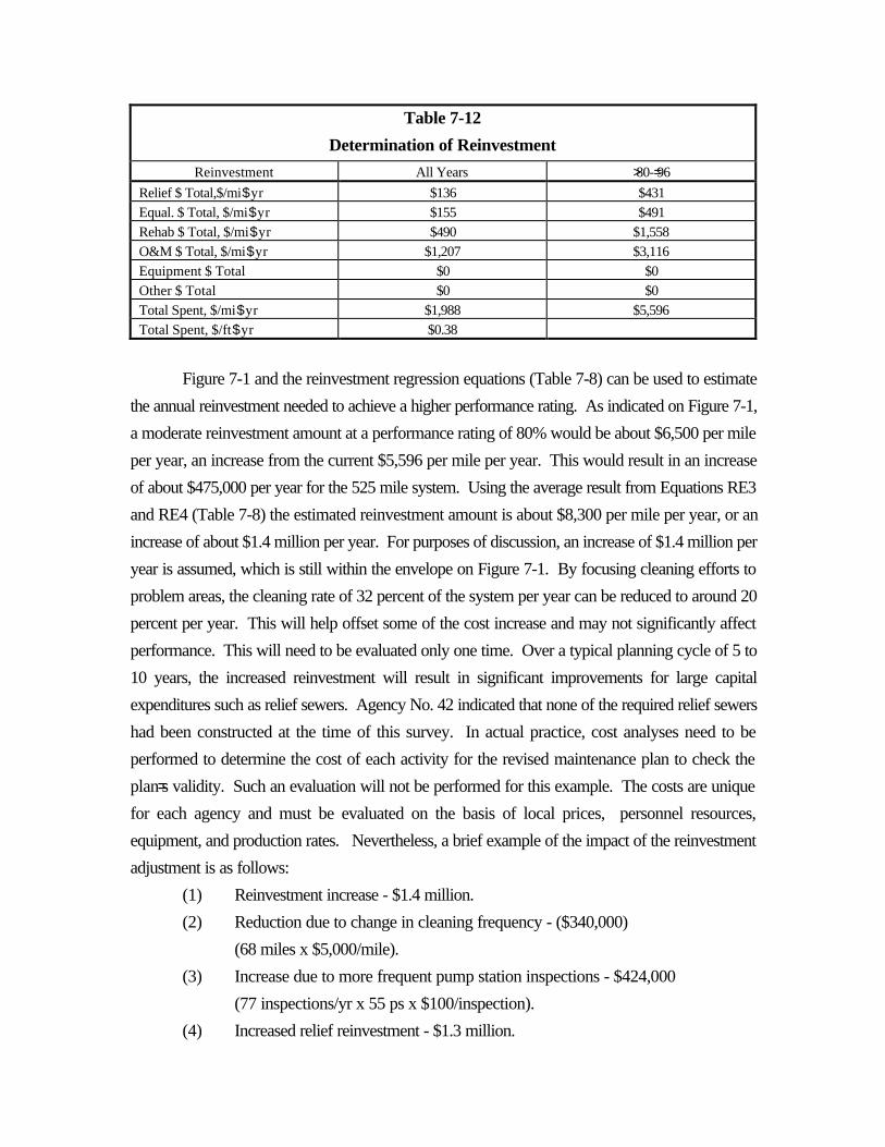
Table 7-12


Reinvestment All Years >80-=96

Relief $ Total,$/mi$yr $136 $431

Equal. $ Total, $/mi$yr $155 $491

Rehab $ Total, $/mi$yr $490 $1,558

O&M $ Total, $/mi$yr $1,207 $3,116

Equipment $ Total $0 $0

Other $ Total $0 $0

Total Spent, $/mi$yr $1,988 $5,596

Total Spent, $/ft$yr $0.38

Figure 7-1 and the reinvestment regression equations (Table 7-8) can be used to estimate

the annual reinvestment needed to achieve a higher performance rating. As indicated on Figure 7-1,

a moderate reinvestment amount at a performance rating of 80% would be about $6,500 per mile

per year, an increase from the current $5,596 per mile per year. This would result in an increase

of about $475,000 per year for the 525 mile system. Using the average result from Equations RE3

and RE4 (Table 7-8) the estimated reinvestment amount is about $8,300 per mile per year, or an

increase of about $1.4 million per year. For purposes of discussion, an increase of $1.4 million per

year is assumed, which is still within the envelope on Figure 7-1. By focusing cleaning efforts to

problem areas, the cleaning rate of 32 percent of the system per year can be reduced to around 20

percent per year. This will help offset some of the cost increase and may not significantly affect

performance. This will need to be evaluated only one time. Over a typical planning cycle of 5 to

10 years, the increased reinvestment will result in significant improvements for large capital

expenditures such as relief sewers. Agency No. 42 indicated that none of the required relief sewers

had been constructed at the time of this survey. In actual practice, cost analyses need to be

performed to determine the cost of each activity for the revised maintenance plan to check the

plan=s validity. Such an evaluation will not be performed for this example. The costs are unique

for each agency and must be evaluated on the basis of local prices, personnel resources,

equipment, and production rates. Nevertheless, a brief example of the impact of the reinvestment

adjustment is as follows:

(1) Reinvestment increase - $1.4 million.

(2) Reduction due to change in cleaning frequency - ($340,000)

(68 miles x $5,000/mile).

(3) Increase due to more frequent pump station inspections - $424,000

(77 inspections/yr x 55 ps x $100/inspection).

(4) Increased relief reinvestment - $1.3 million.

The resulting plan will be a first step towards achieving a system with a maintenance

frequency of about 7.5%, a performance rating of 80%, and a reinvestment of $8,300 per mile per

year.

Refining the maintenance and reinvestment will be an iterative process which will require

judgment to properly address performance deficiencies. The above example provides an approach

to using maintenance frequencies, performance ratings, and system reinvestment amounts in

adjusting a maintenance plan and evaluating its adequacy.

7.6 Conclusion

The data collected during this study and the methods used to develop maintenance

frequencies, performance ratings, and reinvestment rates can be useful in evaluating the adequacy

of existing maintenance programs (including routine maintenance and total reinvestment), and for

making modification and adjustments to these programs. By expressing collection system

maintenance in terms of overall frequency and performance as an overall rating, it is hoped that the

relationship between maintenance (total reinvestment) and system performance will be better

understood. This will also help regulators and agencies evaluate acceptable levels of system

performance and reinvestment.

7.7 Recommendations

This study is a first effort to evaluate the relationship between collection system

performance and maintenance (reinvestment), using an overall rating approach. The data for this

study were difficult to collect, were guessed in some cases, and were not readily available from

many of the agencies surveyed. It is probable that many agencies across the country also lack good

data. It is recommended that agencies compile and keep records of performance and maintenance

(total reinvestment) in a standardized format. The information presented in this study includes

standard formats for collecting and summarizing data. The definitions and guidelines developed

during this study for maintenance, and performance measures should be used by agencies to ensure

uniform interpretation and collection of data.

Specific steps to improve the optimization of collection system maintenance are as follows:

1. Review and refine the maintenance, performance, and reinvestment measures used

in this report. Develop detailed definitions of each.

2. Develop either an information collection guideline which would request that

agencies collect data consistent with results of Step 1 or have a study with a core

group of agencies to provide data that can be used to refine these analyses and to

generate a AGuideline Report for Collection System Maintenance@.

3. Implement the information collection process and analyze the data to develop cost

estimates, maintenance guidelines, and performance measures similar to those

presented in this study.

4. Repeat the analysis on a regular basis every 2-5 years as the output will improve

with the improved data collection.

Appendix A

Questionnaire

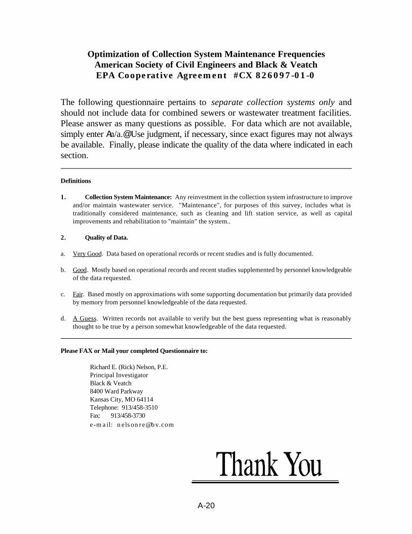
A-20

Optimization of Collection System Maintenance FrequenciesAmerican Society of Civil Engineers and Black & VeatchEPA Cooperative Agreement #CX 826097-01-0

The following questionnaire pertains to separate collection systems only andshould not include data for combined sewers or wastewater treatment facilities.Please answer as many questions as possible. For data which are not available,simply enter An/a.@ Use judgment, if necessary, since exact figures may not alwaysbe available. Finally, please indicate the quality of the data where indicated in eachsection.

Definitions

1. Collection System Maintenance: Any reinvestment in the collection system infrastructure to improveand/or maintain wastewater service. "Maintenance", for purposes of this survey, includes what istraditionally considered maintenance, such as cleaning and lift station service, as well as capitalimprovements and rehabilitation to "maintain" the system..

2. Quality of Data.

a. Very Good. Data based on operational records or recent studies and is fully documented.

b. Good. Mostly based on operational records and recent studies supplemented by personnel knowledgeableof the data requested.

c. Fair. Based mostly on approximations with some supporting documentation but primarily data providedby memory from personnel knowledgeable of the data requested.

d. A Guess. Written records not available to verify but the best guess representing what is reasonablythought to be true by a person somewhat knowledgeable of the data requested.

Please FAX or Mail your completed Questionnaire to:

Richard E. (Rick) Nelson, P.E.Principal InvestigatorBlack & Veatch8400 Ward ParkwayKansas City, MO 64114Telephone: 913/458-3510 Fax: 913/458-3730

e-mail: [email protected]

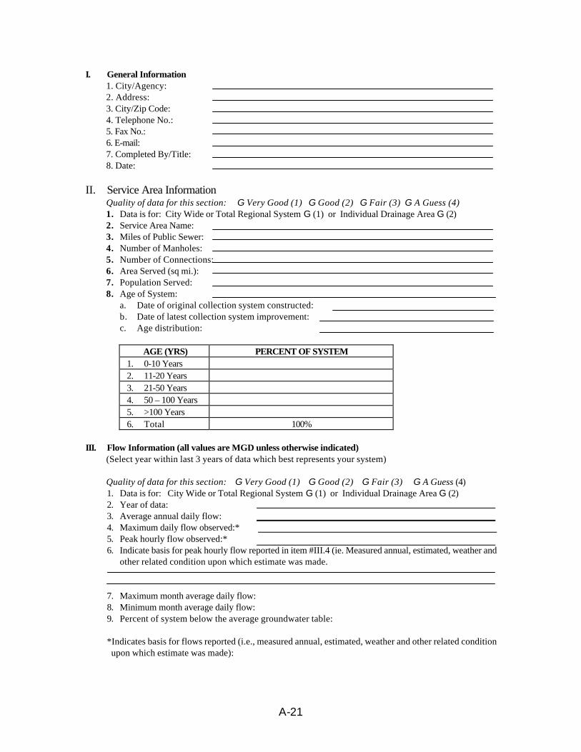
A-21

I. General Information1. City/Agency:2. Address: 3. City/Zip Code: 4. Telephone No.:5. Fax No.:6. E-mail:7. Completed By/Title:8. Date:

II. Service Area InformationQuality of data for this section: G Very Good (1) G Good (2) G Fair (3) G A Guess (4) 1. Data is for: City Wide or Total Regional System G (1) or Individual Drainage Area G (2)2. Service Area Name: 3. Miles of Public Sewer:4. Number of Manholes: 5. Number of Connections:6. Area Served (sq mi.):7. Population Served:8. Age of System:

a. Date of original collection system constructed: b. Date of latest collection system improvement: c. Age distribution:

AGE (YRS) PERCENT OF SYSTEM1. 0-10 Years2. 11-20 Years3. 21-50 Years4. 50 – 100 Years5. >100 Years6. Total 100%

III. Flow Information (all values are MGD unless otherwise indicated)(Select year within last 3 years of data which best represents your system)

Quality of data for this section: G Very Good (1) G Good (2) G Fair (3) G A Guess (4)1. Data is for: City Wide or Total Regional System G (1) or Individual Drainage Area G (2)2. Year of data:3. Average annual daily flow: 4. Maximum daily flow observed:*5. Peak hourly flow observed:*6. Indicate basis for peak hourly flow reported in item #III.4 (ie. Measured annual, estimated, weather and

other related condition upon which estimate was made.

7. Maximum month average daily flow:8. Minimum month average daily flow: 9. Percent of system below the average groundwater table:

*Indicates basis for flows reported (i.e., measured annual, estimated, weather and other related conditionupon which estimate was made):

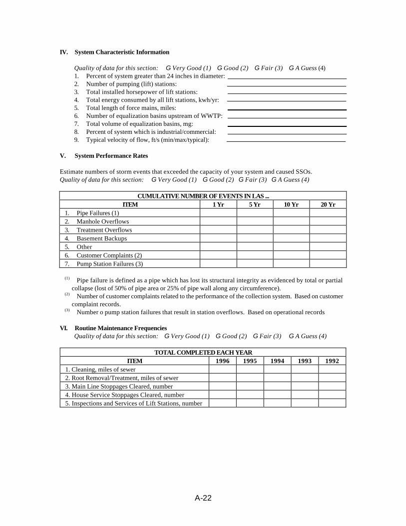
A-22

IV. System Characteristic Information

Quality of data for this section: G Very Good (1) G Good (2) G Fair (3) G A Guess (4)1. Percent of system greater than 24 inches in diameter: 2. Number of pumping (lift) stations:3. Total installed horsepower of lift stations:4. Total energy consumed by all lift stations, kwh/yr:5. Total length of force mains, miles:6. Number of equalization basins upstream of WWTP:7. Total volume of equalization basins, mg:8. Percent of system which is industrial/commercial:9. Typical velocity of flow, ft/s (min/max/typical):

V. System Performance Rates

Estimate numbers of storm events that exceeded the capacity of your system and caused SSOs.Quality of data for this section: G Very Good (1) G Good (2) G Fair (3) G A Guess (4)

CUMULATIVE NUMBER OF EVENTS IN LAS ...ITEM 1 Yr 5 Yr 10 Yr 20 Yr

1. Pipe Failures (1)2. Manhole Overflows3. Treatment Overflows4. Basement Backups5. Other6. Customer Complaints (2)7. Pump Station Failures (3)

(1) Pipe failure is defined as a pipe which has lost its structural integrity as evidenced by total or partialcollapse (lost of 50% of pipe area or 25% of pipe wall along any circumference).

(2) Number of customer complaints related to the performance of the collection system. Based on customercomplaint records.

(3) Number o pump station failures that result in station overflows. Based on operational records

VI. Routine Maintenance FrequenciesQuality of data for this section: G Very Good (1) G Good (2) G Fair (3) G A Guess (4)

TOTAL COMPLETED EACH YEARITEM 1996 1995 1994 1993 1992

1. Cleaning, miles of sewer2. Root Removal/Treatment, miles of sewer3. Main Line Stoppages Cleared, number4. House Service Stoppages Cleared, number5. Inspections and Services of Lift Stations, number

A-23

VII. Inspection Methods Used and Status

Quality of data for this section: G Very Good (1) G Good (2) G Fair (3) G A Guess (4)

INSPECTIONS METHOD AND STATUS (1)

CUMULATIVE PERCENT OF SYSTEM QUANTITYINSPECTED IN LAST ...

INSPECTION TASK 1 YR 5 YR 10 YR 20 YR1. Flow Monitoring/Capacity Evaluation (2)2. Manhole (3)3. Smoke/Dye Test5. Private Sector Building Inspection (4)

(1) Inspection % may exceed 100% of actives have been performed more than once. Percentage should bebase on total quantity of task completed divided by total system. For example, in a system with 100manholes, if 50 manholes were inspected twice each in the last year, the 100% of the system quantitywould have been inspected in the last 1 year; not 50%. This data will help establish the frequency ofinspection activities.

(2) Percent of subsystem (basins) monitored and evaluated.(3) Surface or internal inspections.(4) Inspections for area drains, downspouts, cleanouts, sump discharges and other private sector inflow

sources into the sewer system.

VIII. Approximate Rehabilitation Status Percent Complete:

Quality of data for this section: G Very Good (1) G Good (2) G Fair (3) G A Guess (4)

REHABILITATION TASK PERCENT COMPLETE (1)1. Manhole2. Main line/public service connection repairs3. Relief/equalization4. Private Sector (lateral and illegal disconnect

program)

(1) Indicate the completion status of total estimated rehabilitation required to bring each item to anew or like new condition. For example: (a) if a system requires not rehabilitation (a like newsystem) then all rehabilitation tasks would be 100% complete; (b) in a 100 manhole system, if a totalof 50 manholes require rehabilitation and 25 manholes have already been rehabilitated, then therehabilitation status would be 50% complete; not 25% (i.e. 25/50 – 0.50).

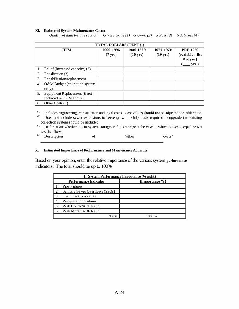
A-24

XI. Estimated System Maintenance Costs:Quality of data for this section: G Very Good (1) G Good (2) G Fair (3) G A Guess (4)

TOTAL DOLLARS SPENT (1)ITEM 1990-1996

(7 yrs)1980-1989

(10 yrs)1970-1970

(10 yrs)PRE-1970

(variable – list# of yrs.)

(____ yrs.)1. Relief (Increased capacity) (2)2. Equalization (2)3. Rehabilitation/replacement4. O&M Budget (collection system

only)5. Equipment Replacement (if not

included in O&M above)6. Other Costs (4)

(1) Includes engineering, construction and legal costs. Cost values should not be adjusted for infiltration.(2) Does not include sewer extensions to serve growth. Only costs required to upgrade the existing

collection system should be included.(3) Differentiate whether it is in-system storage or if it is storage at the WWTP which is used to equalize wet

weather flows.(4) Description of "other costs"

____________________________________________________________

X. Estimated Importance of Performance and Maintenance Activities

Based on your opinion, enter the relative importance of the various system performance

indicators. The total should be up to 100%

1. System Performance Importance (Weight)Performance Indicator (Importance %)

1. Pipe Failures2. Sanitary Sewer Overflows (SSOs)3. Customer Complaints4. Pump Station Failures5. Peak Hourly/ADF Ratio6. Peak Month/ADF Ratio

Total 100%

A-25

X. Estimated Importance of Performance and Maintenance Activities

Based on your opinion, enter the relative importance of the various system performanceindicators. The total should be up to 100%

2. Maintenance Activity Importance (Weight)Maintenance Activity (Importance %)

1. % System Cleaned/Yr2. % System Root Removal/Yr3. Lift Station Service4. Flow Monitoring/Capacity Evaluation5. Manhole Inspection6. Smoke/Dye Testing7. CCTV Inspections8. Private Sector Inspections9. Manhole Rehabilitation10. Main Line Rehabilitation11. Relief Sewer Construction12. Private Sector I/I Source Removal

Total 100%

XI. Effectiveness of Program:

1. Are you satisfied with your system maintenance (total reinvestment) program:

a. Strongly Agree _____ (system performance is as required, cost effective budget)

b. Agree _____ (system performance is generally as required, budgetadequate)

c. Not Sure _____ (system performance not defined, budget may be adequate)

d. Disagree _____ (system performance generally not as required, budget notadequate)

e. Strongly Disagree _____ (system performance and budget unacceptable)

2. What would you do different, if anything?______________________________________________________________________________________________________________________________________________________________________________________________________________________________________________________________________________________________________________________________________________________________________________________________________________________________________________________________________________________________________________________________

Appendix B

Data Provided by Respondents

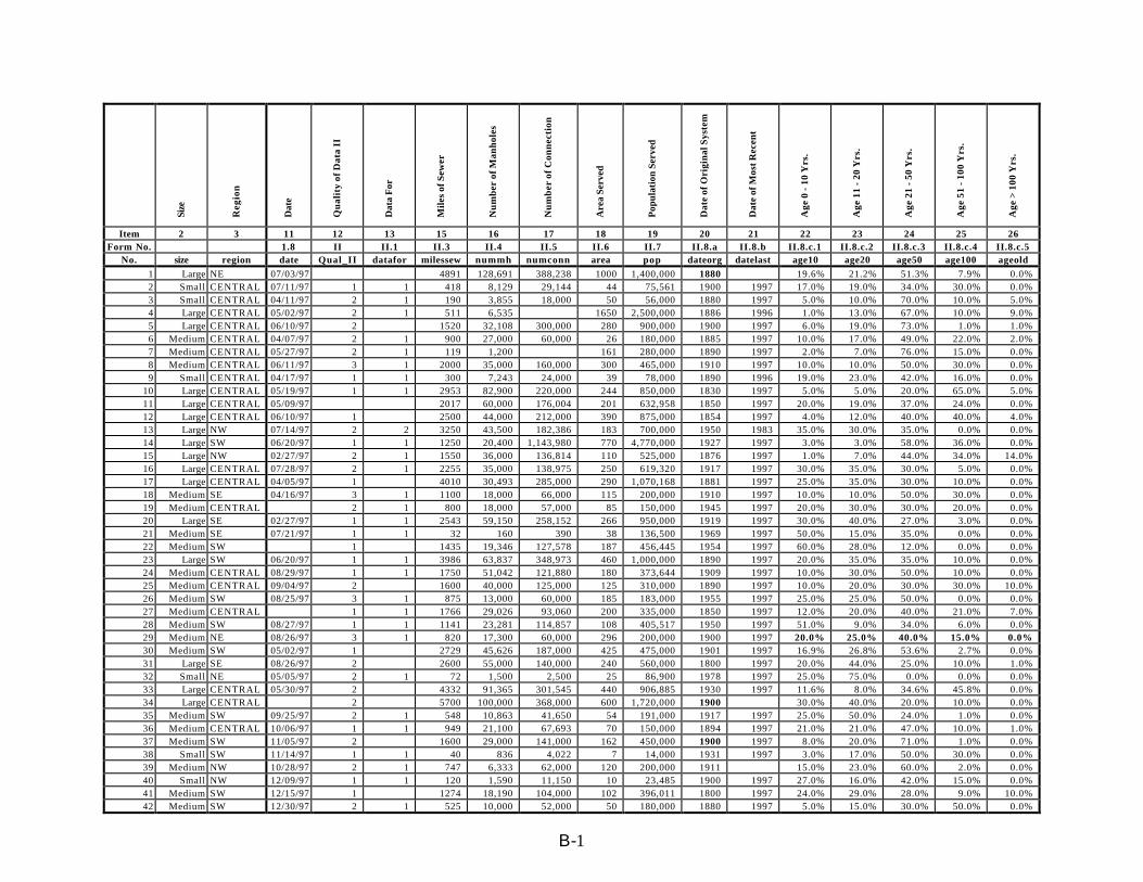
B-1

Size

Reg

ion

Dat

e

Qu

alit

y of

Dat

a II

Dat

a F

or

Mil

es o

f S

ewer

Nu

mb

er o

f M

anh

oles

Nu

mb

er o

f C

onn

ecti

on

Are

a Se

rved

Pop

ula

tion

Ser

ved

Dat

e of

Ori

gin

al S

yste

m

Dat

e of

Mos

t R

ecen

t

Age

0 -

10

Yrs

.

Age

11

- 20

Yrs

.

Age

21

- 50

Yrs

.

Age

51

- 10

0 Y

rs.

Age

> 1

00 Y

rs.

Item 2 3 11 12 13 15 16 17 18 19 20 21 22 23 24 25 26Form No. 1.8 II II.1 II.3 II.4 II.5 II.6 II.7 II.8.a II.8.b II.8.c.1 II.8.c.2 II.8.c.3 II.8.c.4 II.8.c.5

No. size region date Qual_II datafor milessew nummh numconn area pop dateorg datelast age10 age20 age50 age100 ageold

1 Large NE 07/03/97 4891 128,691 388,238 1000 1,400,000 1880 19.6% 21.2% 51.3% 7.9% 0.0%2 Small CENTRAL 07/11/97 1 1 418 8,129 29,144 44 75,561 1900 1997 17.0% 19.0% 34.0% 30.0% 0.0%3 Small CENTRAL 04/11/97 2 1 190 3,855 18,000 50 56,000 1880 1997 5.0% 10.0% 70.0% 10.0% 5.0%4 Large CENTRAL 05/02/97 2 1 511 6,535 1650 2,500,000 1886 1996 1.0% 13.0% 67.0% 10.0% 9.0%5 Large CENTRAL 06/10/97 2 1520 32,108 300,000 280 900,000 1900 1997 6.0% 19.0% 73.0% 1.0% 1.0%6 Medium CENTRAL 04/07/97 2 1 900 27,000 60,000 26 180,000 1885 1997 10.0% 17.0% 49.0% 22.0% 2.0%7 Medium CENTRAL 05/27/97 2 1 119 1,200 161 280,000 1890 1997 2.0% 7.0% 76.0% 15.0% 0.0%8 Medium CENTRAL 06/11/97 3 1 2000 35,000 160,000 300 465,000 1910 1997 10.0% 10.0% 50.0% 30.0% 0.0%9 Small CENTRAL 04/17/97 1 1 300 7,243 24,000 39 78,000 1890 1996 19.0% 23.0% 42.0% 16.0% 0.0%

10 Large CENTRAL 05/19/97 1 1 2953 82,900 220,000 244 850,000 1830 1997 5.0% 5.0% 20.0% 65.0% 5.0%11 Large CENTRAL 05/09/97 2017 60,000 176,004 201 632,958 1850 1997 20.0% 19.0% 37.0% 24.0% 0.0%12 Large CENTRAL 06/10/97 1 2500 44,000 212,000 390 875,000 1854 1997 4.0% 12.0% 40.0% 40.0% 4.0%13 Large NW 07/14/97 2 2 3250 43,500 182,386 183 700,000 1950 1983 35.0% 30.0% 35.0% 0.0% 0.0%14 Large SW 06/20/97 1 1 1250 20,400 1,143,980 770 4,770,000 1927 1997 3.0% 3.0% 58.0% 36.0% 0.0%15 Large NW 02/27/97 2 1 1550 36,000 136,814 110 525,000 1876 1997 1.0% 7.0% 44.0% 34.0% 14.0%16 Large CENTRAL 07/28/97 2 1 2255 35,000 138,975 250 619,320 1917 1997 30.0% 35.0% 30.0% 5.0% 0.0%17 Large CENTRAL 04/05/97 1 4010 30,493 285,000 290 1,070,168 1881 1997 25.0% 35.0% 30.0% 10.0% 0.0%18 Medium SE 04/16/97 3 1 1100 18,000 66,000 115 200,000 1910 1997 10.0% 10.0% 50.0% 30.0% 0.0%19 Medium CENTRAL 2 1 800 18,000 57,000 85 150,000 1945 1997 20.0% 30.0% 30.0% 20.0% 0.0%20 Large SE 02/27/97 1 1 2543 59,150 258,152 266 950,000 1919 1997 30.0% 40.0% 27.0% 3.0% 0.0%21 Medium SE 07/21/97 1 1 32 160 390 38 136,500 1969 1997 50.0% 15.0% 35.0% 0.0% 0.0%22 Medium SW 1 1435 19,346 127,578 187 456,445 1954 1997 60.0% 28.0% 12.0% 0.0% 0.0%23 Large SW 06/20/97 1 1 3986 63,837 348,973 460 1,000,000 1890 1997 20.0% 35.0% 35.0% 10.0% 0.0%24 Medium CENTRAL 08/29/97 1 1 1750 51,042 121,880 180 373,644 1909 1997 10.0% 30.0% 50.0% 10.0% 0.0%25 Medium CENTRAL 09/04/97 2 1600 40,000 125,000 125 310,000 1890 1997 10.0% 20.0% 30.0% 30.0% 10.0%26 Medium SW 08/25/97 3 1 875 13,000 60,000 185 183,000 1955 1997 25.0% 25.0% 50.0% 0.0% 0.0%27 Medium CENTRAL 1 1 1766 29,026 93,060 200 335,000 1850 1997 12.0% 20.0% 40.0% 21.0% 7.0%28 Medium SW 08/27/97 1 1 1141 23,281 114,857 108 405,517 1950 1997 51.0% 9.0% 34.0% 6.0% 0.0%29 Medium NE 08/26/97 3 1 820 17,300 60,000 296 200,000 1900 1997 20.0% 25.0% 40.0% 15.0% 0.0%30 Medium SW 05/02/97 1 2729 45,626 187,000 425 475,000 1901 1997 16.9% 26.8% 53.6% 2.7% 0.0%31 Large SE 08/26/97 2 2600 55,000 140,000 240 560,000 1800 1997 20.0% 44.0% 25.0% 10.0% 1.0%32 Small NE 05/05/97 2 1 72 1,500 2,500 25 86,900 1978 1997 25.0% 75.0% 0.0% 0.0% 0.0%33 Large CENTRAL 05/30/97 2 4332 91,365 301,545 440 906,885 1930 1997 11.6% 8.0% 34.6% 45.8% 0.0%34 Large CENTRAL 2 5700 100,000 368,000 600 1,720,000 1900 30.0% 40.0% 20.0% 10.0% 0.0%35 Medium SW 09/25/97 2 1 548 10,863 41,650 54 191,000 1917 1997 25.0% 50.0% 24.0% 1.0% 0.0%36 Medium CENTRAL 10/06/97 1 1 949 21,100 67,693 70 150,000 1894 1997 21.0% 21.0% 47.0% 10.0% 1.0%37 Medium SW 11/05/97 2 1600 29,000 141,000 162 450,000 1900 1997 8.0% 20.0% 71.0% 1.0% 0.0%38 Small SW 11/14/97 1 1 40 836 4,022 7 14,000 1931 1997 3.0% 17.0% 50.0% 30.0% 0.0%39 Medium NW 10/28/97 2 1 747 6,333 62,000 120 200,000 1911 15.0% 23.0% 60.0% 2.0% 0.0%40 Small NW 12/09/97 1 1 120 1,590 11,150 10 23,485 1900 1997 27.0% 16.0% 42.0% 15.0% 0.0%41 Medium SW 12/15/97 1 1274 18,190 104,000 102 396,011 1800 1997 24.0% 29.0% 28.0% 9.0% 10.0%42 Medium SW 12/30/97 2 1 525 10,000 52,000 50 180,000 1880 1997 5.0% 15.0% 30.0% 50.0% 0.0%

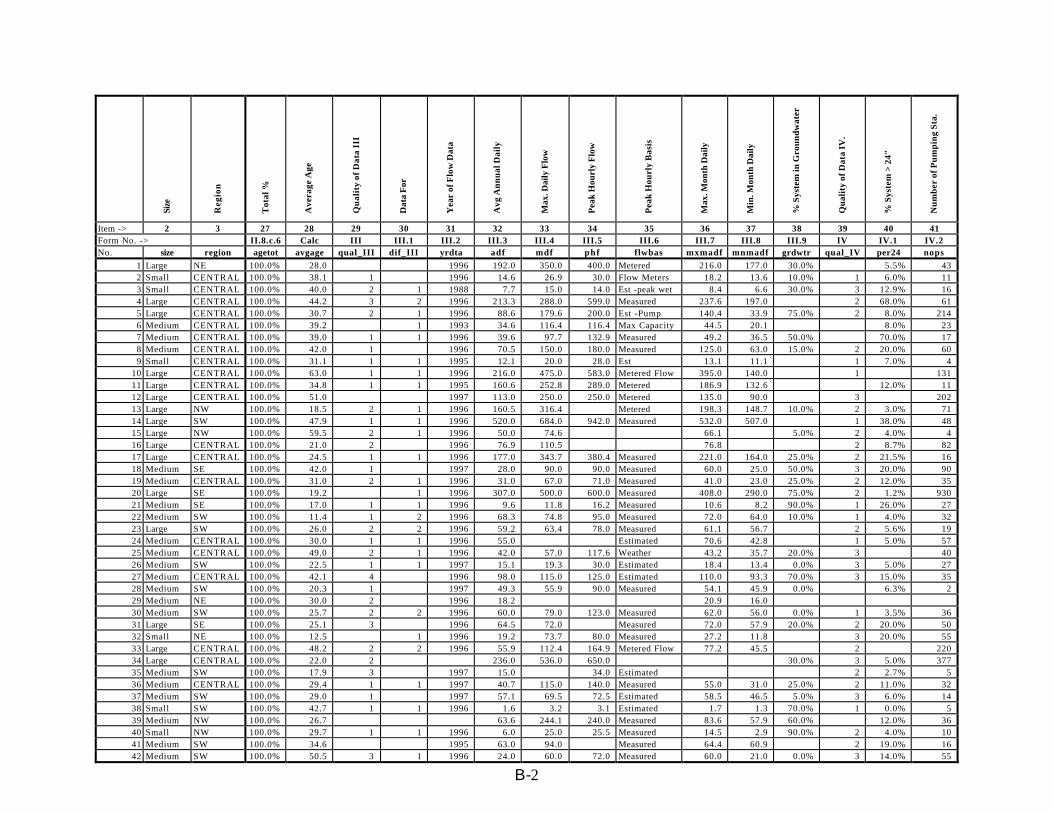
B-2

Size

Reg

ion

Tot

al %

Ave

rage

Age

Qu

alit

y of

Dat

a II

I

Dat

a F

or

Yea

r of

Flo

w D

ata

Avg

An

nu

al D

aily

Max

. Dai

ly F

low

Pea

k H

ourl

y F

low

Pea

k H

ourl

y B

asis

Max

. Mon

th D

aily

Min

. Mon

th D

aily

% S

yste

m in

Gro

un

dw

ater

Qu

alit

y of

Dat

a IV

.

% S

yste

m >

24"

Nu

mb

er o

f P

um

pin

g S

ta.

Item -> 2 3 27 28 29 30 31 32 33 34 35 36 37 38 39 40 41Form No. -> II.8.c.6 Calc III III.1 III.2 III.3 III.4 III.5 III.6 III.7 III.8 III.9 IV IV.1 IV.2No. size region agetot avgage qual_III dif_III yrdta adf mdf phf flwbas mxmadf mnmadf grdwtr qual_IV per24 nops

1 Large NE 100.0% 28.0 1996 192.0 350.0 400.0 Metered 216.0 177.0 30.0% 5.5% 432 Small CENTRAL 100.0% 38.1 1 1996 14.6 26.9 30.0 Flow Meters 18.2 13.6 10.0% 1 6.0% 113 Small CENTRAL 100.0% 40.0 2 1 1988 7.7 15.0 14.0 Est -peak wet 8.4 6.6 30.0% 3 12.9% 164 Large CENTRAL 100.0% 44.2 3 2 1996 213.3 288.0 599.0 Measured 237.6 197.0 2 68.0% 615 Large CENTRAL 100.0% 30.7 2 1 1996 88.6 179.6 200.0 Est -Pump 140.4 33.9 75.0% 2 8.0% 2146 Medium CENTRAL 100.0% 39.2 1 1993 34.6 116.4 116.4 Max Capacity 44.5 20.1 8.0% 237 Medium CENTRAL 100.0% 39.0 1 1 1996 39.6 97.7 132.9 Measured 49.2 36.5 50.0% 70.0% 178 Medium CENTRAL 100.0% 42.0 1 1996 70.5 150.0 180.0 Measured 125.0 63.0 15.0% 2 20.0% 609 Small CENTRAL 100.0% 31.1 1 1 1995 12.1 20.0 28.0 Est 13.1 11.1 1 7.0% 4

10 Large CENTRAL 100.0% 63.0 1 1 1996 216.0 475.0 583.0 Metered Flow 395.0 140.0 1 13111 Large CENTRAL 100.0% 34.8 1 1 1995 160.6 252.8 289.0 Metered 186.9 132.6 12.0% 1112 Large CENTRAL 100.0% 51.0 1997 113.0 250.0 250.0 Metered 135.0 90.0 3 20213 Large NW 100.0% 18.5 2 1 1996 160.5 316.4 Metered 198.3 148.7 10.0% 2 3.0% 7114 Large SW 100.0% 47.9 1 1 1996 520.0 684.0 942.0 Measured 532.0 507.0 1 38.0% 4815 Large NW 100.0% 59.5 2 1 1996 50.0 74.6 66.1 5.0% 2 4.0% 416 Large CENTRAL 100.0% 21.0 2 1996 76.9 110.5 76.8 2 8.7% 8217 Large CENTRAL 100.0% 24.5 1 1 1996 177.0 343.7 380.4 Measured 221.0 164.0 25.0% 2 21.5% 1618 Medium SE 100.0% 42.0 1 1997 28.0 90.0 90.0 Measured 60.0 25.0 50.0% 3 20.0% 9019 Medium CENTRAL 100.0% 31.0 2 1 1996 31.0 67.0 71.0 Measured 41.0 23.0 25.0% 2 12.0% 3520 Large SE 100.0% 19.2 1 1996 307.0 500.0 600.0 Measured 408.0 290.0 75.0% 2 1.2% 93021 Medium SE 100.0% 17.0 1 1 1996 9.6 11.8 16.2 Measured 10.6 8.2 90.0% 1 26.0% 2722 Medium SW 100.0% 11.4 1 2 1996 68.3 74.8 95.0 Measured 72.0 64.0 10.0% 1 4.0% 3223 Large SW 100.0% 26.0 2 2 1996 59.2 63.4 78.0 Measured 61.1 56.7 2 5.6% 1924 Medium CENTRAL 100.0% 30.0 1 1 1996 55.0 Estimated 70.6 42.8 1 5.0% 5725 Medium CENTRAL 100.0% 49.0 2 1 1996 42.0 57.0 117.6 Weather 43.2 35.7 20.0% 3 4026 Medium SW 100.0% 22.5 1 1 1997 15.1 19.3 30.0 Estimated 18.4 13.4 0.0% 3 5.0% 2727 Medium CENTRAL 100.0% 42.1 4 1996 98.0 115.0 125.0 Estimated 110.0 93.3 70.0% 3 15.0% 3528 Medium SW 100.0% 20.3 1 1997 49.3 55.9 90.0 Measured 54.1 45.9 0.0% 6.3% 229 Medium NE 100.0% 30.0 2 1996 18.2 20.9 16.030 Medium SW 100.0% 25.7 2 2 1996 60.0 79.0 123.0 Measured 62.0 56.0 0.0% 1 3.5% 3631 Large SE 100.0% 25.1 3 1996 64.5 72.0 Measured 72.0 57.9 20.0% 2 20.0% 5032 Small NE 100.0% 12.5 1 1996 19.2 73.7 80.0 Measured 27.2 11.8 3 20.0% 5533 Large CENTRAL 100.0% 48.2 2 2 1996 55.9 112.4 164.9 Metered Flow 77.2 45.5 2 22034 Large CENTRAL 100.0% 22.0 2 236.0 536.0 650.0 30.0% 3 5.0% 37735 Medium SW 100.0% 17.9 3 1997 15.0 34.0 Estimated 2 2.7% 536 Medium CENTRAL 100.0% 29.4 1 1 1997 40.7 115.0 140.0 Measured 55.0 31.0 25.0% 2 11.0% 3237 Medium SW 100.0% 29.0 1 1997 57.1 69.5 72.5 Estimated 58.5 46.5 5.0% 3 6.0% 1438 Small SW 100.0% 42.7 1 1 1996 1.6 3.2 3.1 Estimated 1.7 1.3 70.0% 1 0.0% 539 Medium NW 100.0% 26.7 63.6 244.1 240.0 Measured 83.6 57.9 60.0% 12.0% 3640 Small NW 100.0% 29.7 1 1 1996 6.0 25.0 25.5 Measured 14.5 2.9 90.0% 2 4.0% 1041 Medium SW 100.0% 34.6 1995 63.0 94.0 Measured 64.4 60.9 2 19.0% 1642 Medium SW 100.0% 50.5 3 1 1996 24.0 60.0 72.0 Measured 60.0 21.0 0.0% 3 14.0% 55

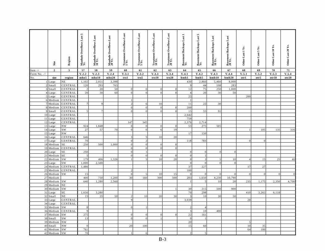
B-3

Size

Reg

ion

Man

hol

e O

verf

low

s L

ast

5Y

r.

Man

hol

e O

verf

low

s L

ast

10 Y

r.

Man

hol

e O

verf

low

s L

ast

20 Y

r.

Tre

atm

ent

Ove

rflo

ws

Las

t1

Yr.

Tre

atm

ent

Ove

rflo

ws

Las

t5

Yr.

Tre

atm

ent

Ove

rflo

ws

Las

t10

Yr.

Tre

atm

ent

Ove

rflo

ws

Las

t20

Yr.

Bas

emen

t B

ack

up

s L

ast

1Y

r.

Bas

emen

t B

ack

up

s L

ast

5Y

r.

Bas

emen

t B

ack

up

s L

ast

10 Y

r.

Bas

emen

t B

ack

up

s L

ast

20 Y

r.

Oth

er L

ast 1

Yr.

Oth

er L

ast 5

Yr.

Oth

er L

ast

10 Y

r.

Oth

er L

ast

20 Y

r.

Item -> 2 3 57 58 59 60 61 62 63 64 65 66 67 68 69 70 71Form No. -> V.2.2 V.2.3 V.2.4 V.3.1 V.3.2 V.3.3 V.3.4 V.4.1 V.4.2 V.4.3 V.4.4 V.5.1 V.5.2 V.5.3 V.5.4No. size region mho5 mho10 mho20 tro1 tro5 tro10 tro20 bmb1 bmb5 bmb10 bmb20 otr1 otr5 otr10 otr20

1 Large NE 1,102 2,051 3,398 430 2,860 5,460 8,0002 Small CENTRAL 120 293 765 9 44 108 2833 Small CENTRAL 2 20 50 0 0 0 0 12 75 250 1,0004 Large CENTRAL 20 30 60 0 0 0 0 4 20 30 505 Large CENTRAL 25 2006 Medium CENTRAL 1 17 Medium CENTRAL 7 9 2 6 10 11 22 308 Medium CENTRAL 0 0 0 0 2009 Small CENTRAL 5 7 0 0 0 0 15 55 91

10 Large CENTRAL 2,64211 Large CENTRAL 75912 Large CENTRAL 147 345 2,376 2,71413 Large NW 924 1,848 0 0 0 0 53 275 50514 Large SW 27 57 70 0 0 6 19 1 105 135 31615 Large NW 17 15016 Large CENTRAL 646 3 5 10 2017 Large CENTRAL 70 0 2 118 783 0 018 Medium SE 250 500 1,000 0 0 0 019 Medium CENTRAL 0 0 0 020 Large SE 250 0 1 0 0 0 021 Medium SE 5 0 0 0 0 0 122 Medium SW 179 406 1,326 1 5 10 20 0 3 5 10 4 15 25 4023 Large SW 1,000 2,500 0 0 0 024 Medium CENTRAL 1,486 37 227 17 2725 Medium CENTRAL 2 10026 Medium SW 15 0 5 10 15 0 0 0 0 0 0 0 027 Medium 400 750 1,200 30 160 300 500 283 1,650 4,230 10,79028 Medium SW 640 1,280 2,560 1 5 10 20 235 1,175 2,350 4,70029 Medium NE30 Medium SW 1 30 215 500 90031 Large SE 1,656 3,280 70 298 410 3,265 6,11832 Small NE 15 35 50 2 10 20 30 3 10 30 5033 Large CENTRAL 9 3,039 2834 Large CENTRAL35 Medium SW 8 0 1 2 436 Medium CENTRAL 9 3 10 40037 Medium SW 275 0 0 0 0 22 16138 Small SW 13 0 0 1 0 139 Medium NW 20 540 Small NW 0 20 100 15 60 10 3541 Medium SW 761 64 10042 Medium SW 70 1 6 2 5

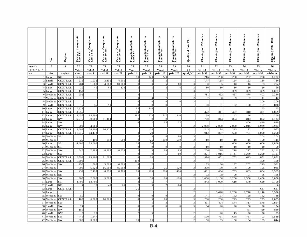
B-4

Size

Reg

ion

Cu

stom

er C

omp

lain

tsL

ast

1 Y

r.

Cu

stom

er C

omp

lain

tsL

ast

5 Y

rs.

Cu

stom

er C

omp

lain

tsL

ast

10 Y

rs.

Cu

stom

er C

omp

lain

tsL

ast

20 Y

rs.

Pu

mp

Sta

tion

Fai

lure

sL

ast

1 Y

r.

Pu

mp

Sta

tion

Fai

lure

sL

ast

5 Y

rs.

Pu

mp

Sta

tion

Fai

lure

sL

ast

10 Y

rs.

Pu

mp

Sta

tion

Fai

lure

sL

ast

20 Y

rs.

Qu

alit

y of

Dat

a V

I.

Cle

anin

g in

199

2, m

iles

Cle

anin

g in

199

3, m

iles

Cle

anin

g in

199

4, m

iles

Cle

anin

g in

199

5, m

iles

Cle

anin

g in

199

6, m

iles

Cle

anin

g 19

92 -

1996

,m

iles

Item -> 2 3 72 73 74 75 76 77 78 79 80 81 82 83 84 85 86Form No. -> V.6.1 V.6.2 V.6.3 V.6.4 V.7.1 V.7.2 V.7.3 V.7.4 VI VI.1.1 VI.1.2 VI.1.3 VI.1.4 VI.1.5 VI.1.6No. size region cust1 cust5 cust10 cust20 psfail1 psfail5 psfail10 psfail20 qual_VI micln92 micln93 micln94 micln95 micln96 miclntot

1 Large NE 6,241 10 123 223 1 216 238 268 262 298 1,2822 Small CENTRAL 216 1,032 2,151 4,501 1 2 2 1 177 135 168 162 138 7803 Small CENTRAL 284 1,600 4,000 10,000 0 3 5 10 3 30 35 40 46 53 2044 Large CENTRAL 20 40 80 120 1 1 2 4 2 10 10 10 10 10 505 Large CENTRAL 150 3 359 359 359 1,0776 Medium CENTRAL 251 3 1 511 452 437 478 402 2,2807 Medium CENTRAL 3 4 7 2 7 8 9 7 11 428 Medium CENTRAL 0 0 0 0 3 200 2009 Small CENTRAL 15 55 91 0 0 0 1 180 151 152 168 177 828

10 Large CENTRAL 7,823 65 346 1 95 9511 Large CENTRAL 3,555 14 1 422 341 407 318 381 1,86912 Large CENTRAL 5,457 18,991 281 623 747 840 1 39 41 42 46 101 26913 Large NW 6,616 30,009 51,484 0 0 0 1 760 844 854 813 852 4,12314 Large SW 0 1 15 32 1 400 449 84915 Large NW 800 4,000 2 2,000 2,000 2,000 2,045 1,939 9,98416 Large CENTRAL 5,668 34,901 86,924 36 1 245 174 225 172 137 95317 Large CENTRAL 11,975 44,172 3 28 1 912 887 678 781 1,000 4,25818 Medium SE 1 3 8 10 3 204 20419 Medium 25 100 250 500 2 25 100 500 2 10 10 10 15 100 14520 Large SE 4,600 23,000 14 70 1 600 600 600 1,80021 Medium SE 0 0 0 0 3 10 10 10 10 10 5022 Medium SW 640 2,981 4,998 8,625 1 5 10 15 2 206 228 218 227 232 1,11123 Large SW 0 0 5 10 2 821 1,016 1,141 1,239 1,200 5,41724 Medium CENTRAL 2,593 13,402 21,095 0 20 2 974 651 752 623 851 3,85125 Medium CENTRAL 1,200 100 2 400 40026 Medium SW 250 1,500 3,000 6,000 0 2 1 183 190 197 202 219 99127 Medium 900 6,320 16,000 45,000 4 35 75 120 2 200 180 170 190 195 93528 Medium SW 439 2,195 4,390 8,780 20 100 200 400 1 481 634 783 863 804 3,56529 Medium NE 2 92 108 99 101 86 48630 Medium SW 300 2,000 5,000 4 30 80 160 2 1,000 1,100 1,200 1,300 1,400 6,00031 Large SE 4,700 18,700 2 5 7 1 843 1,090 619 579 629 3,76032 Small NE 4 10 40 60 2 5 7 14 033 Large CENTRAL 26 2 637 63734 Large 2 3,420 2,280 1,710 1,140 8,55035 Medium SW 55 0 0 0 2 141 157 132 128 182 73936 Medium CENTRAL 1,100 6,500 10,200 0 5 10 3 200 200 225 225 225 1,07537 Medium SW 1 2 2 481 494 544 717 578 2,81438 Small SW 24 0 0 0 0 3 34 20 20 30 20 12439 Medium NW 150 1 451 429 88040 Small NW 8 25 2 5 2 20 15 20 20 7541 Medium SW 749 1,347 2 590 751 668 737 793 3,53942 Medium SW 800 3,800 10 60 2 150 165 150 184 195 844

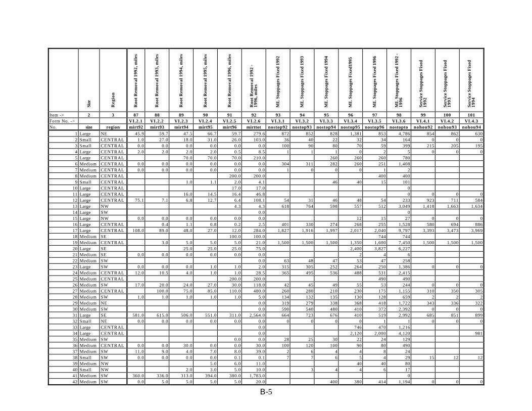
B-5

Size

Reg

ion

Roo

t R

emov

al 1

992,

mil

es

Roo

t R

emov

al 1

993,

mil

es

Roo

t R

emov

al 1

994,

mil

es

Roo

t R

emov

al 1

995,

mil

es

Roo

t R

emov

al 1

996,

mil

es

Roo

t R

emov

al 1

992

-19

96, m

iles

ML

Sto

pp

ages

Fix

ed 1

992

ML

Sto

pp

ages

Fix

ed 1

993

ML

Sto

pp

ages

Fix

ed 1

994

ML

Sto

pp

ages

Fix

ed19

95

ML

Sto

pp

ages

Fix

ed 1

996

ML

Sto

pp

ages

Fix

ed 1

992

-19

96

Ser

vice

Sto

pp

ages

Fix

ed19

92

Ser

vice

Sto

pp

ages

Fix

ed19

93

Ser

vice

Sto

pp

ages

Fix

ed19

94

Item -> 2 3 87 88 89 90 91 92 93 94 95 96 97 98 99 100 101Form No. -> VI.2.1 VI.2.2 VI.2.3 VI.2.4 VI.2.5 VI.2.6 VI.3.1 VI.3.2 VI.3.3 VI.3.4 VI.3.5 VI.3.6 VI.4.1 VI.4.2 VI.4.3No. size region mirt92 mirt93 mirt94 mirt95 mirt96 mirttot nostop92 nostop93 nostop94 nostop95 nostop96 nostopto nohou92 nohou93 nohou94

1 Large NE 45.9 59.7 47.5 66.7 59.7 279.6 872 852 828 1,381 853 4,786 854 862 6302 Small CENTRAL 1.0 27.0 18.0 31.0 26.0 103.0 36 40 22 32 34 164 0 0 03 Small CENTRAL 0.0 0.0 0.0 0.0 0.0 0.0 100 90 80 70 59 399 215 205 1954 Large CENTRAL 2.0 2.0 2.0 2.0 0.5 8.5 1 1 1 0 2 5 0 0 05 Large CENTRAL 70.0 70.0 70.0 210.0 260 260 260 7806 Medium CENTRAL 0.0 0.0 0.0 0.0 0.0 0.0 304 311 282 260 251 1,4087 Medium CENTRAL 0.0 0.0 0.0 0.0 0.0 0.0 1 0 0 0 1 28 Medium CENTRAL 200.0 200.0 400 4009 Small CENTRAL 1.0 1.1 2.0 4.1 46 40 15 101

10 Large CENTRAL 17.0 17.0 011 Large CENTRAL 16.0 14.5 16.4 46.8 0 0 0 012 Large CENTRAL 75.1 7.1 6.8 12.7 6.4 108.1 54 31 46 48 54 233 923 711 58413 Large NW 4.3 4.3 618 764 598 557 512 3,049 1,418 1,663 1,63414 Large SW 0.0 015 Large NW 0.0 0.0 0.0 0.0 0.0 0.0 12 15 27 0 0 016 Large CENTRAL 0.4 1.1 0.8 0.2 2.5 401 330 274 268 255 1,528 580 694 88617 Large CENTRAL 108.0 89.0 48.0 27.0 12.0 284.0 1,827 1,916 1,997 2,017 2,040 9,797 3,393 3,473 3,96918 Medium SE 100.0 100.0 744 74419 Medium CENTRAL 3.0 5.0 5.0 5.0 21.0 1,500 1,500 1,500 1,350 1,600 7,450 1,500 1,500 1,50020 Large SE 25.0 25.0 25.0 75.0 2,400 3,827 6,22721 Medium SE 0.0 0.0 0.0 0.0 0.0 0.0 2 4 622 Medium SW 0.0 63 48 47 53 47 25823 Large SW 0.0 0.0 0.0 1.0 1.0 2.0 315 305 252 264 250 1,386 0 0 024 Medium CENTRAL 12.0 10.5 4.0 1.0 1.0 28.5 365 495 536 488 531 2,41525 Medium CENTRAL 200.0 200.0 490 49026 Medium SW 17.0 20.0 24.0 27.0 30.0 118.0 42 45 49 55 53 244 0 0 027 Medium CENTRAL 100.0 75.0 85.0 110.0 480.0 260 280 210 230 175 1,155 310 350 30528 Medium SW 1.0 1.0 1.0 1.0 1.0 5.0 134 132 135 130 128 659 2 2 229 Medium NE 0.0 319 279 338 368 418 1,722 343 336 32230 Medium SW 0.0 590 540 480 410 372 2,392 0 0 031 Large SE 581.0 615.0 506.0 551.0 311.0 2,564.0 664 723 676 410 519 2,992 685 851 89932 Small NE 0.0 0.0 0.0 0.0 0.0 0.0 0 0 0 0 1 1 0 0 033 Large CENTRAL 0.0 746 470 1,21634 Large CENTRAL 0.0 2,120 2,000 4,120 98135 Medium SW 0.0 0.0 28 25 30 22 24 12936 Medium CENTRAL 0.0 0.0 30.0 0.0 0.0 30.0 100 120 100 90 80 49037 Medium SW 11.0 9.0 4.0 7.0 8.0 39.0 2 6 4 4 8 2438 Small SW 0.0 0.0 0.0 0.0 0.1 0.1 7 7 6 5 4 29 15 12 1239 Medium NW 5.0 6.0 11.0 40 40 8040 Small NW 2.0 3.0 5.0 10.0 3 4 4 6 1741 Medium SW 360.0 336.0 313.0 394.0 380.0 1,783.0 042 Medium SW 0.0 5.0 5.0 5.0 5.0 20.0 400 380 414 1,194 0 0 0

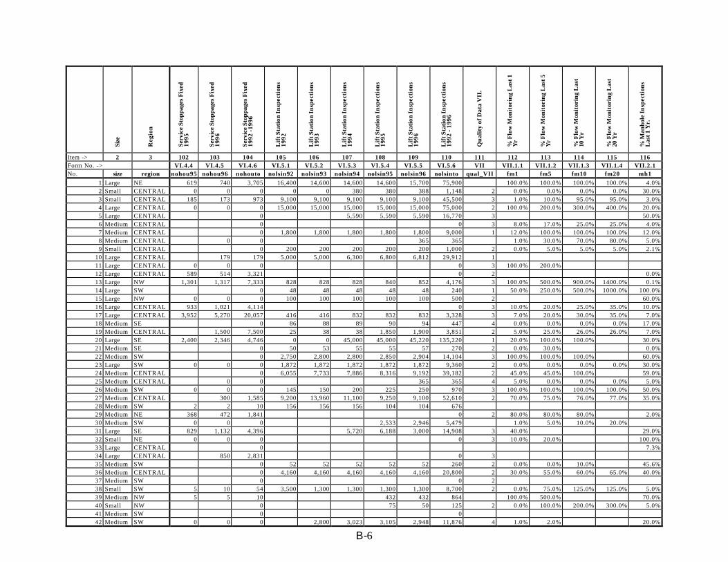
B-6

Size

Reg

ion

Ser

vice

Sto

pp

ages

Fix

ed19

95

Ser

vice

Sto

pp

ages

Fix

ed19

96

Ser

vice

Sto

pp

ages

Fix

ed19

92 -

1996

Lif

t S

tati

on I

nsp

ecti

ons

1992

Lif

t S

tati

on I

nsp

ecti

ons

1993

Lif

t S

tati

on I

nsp

ecti

ons

1994

Lif

t S

tati

on I

nsp

ecti

ons

1995

Lif

t S

tati

on I

nsp

ecti

ons

1996

Lif

t S

tati

on I

nsp

ecti

ons

1992

- 1

996

Qu

alit

y of

Dat

a V

II.

% F

low

Mon

itor

ing

Las

t 1

Yr

% F

low

Mon

itor

ing

Las

t 5

Yr

% F

low

Mon

itor

ing

Las

t10

Yr

% F

low

Mon

itor

ing

Las

t20

Yr

% M

anh

ole

Insp

ecti

ons

Las

t 1

Yr.

Item -> 2 3 102 103 104 105 106 107 108 109 110 111 112 113 114 115 116Form No. -> VI.4.4 VI.4.5 VI.4.6 VI.5.1 VI.5.2 VI.5.3 VI.5.4 VI.5.5 VI.5.6 VII VII.1.1 VII.1.2 VII.1.3 VII.1.4 VII.2.1No. size region nohou95 nohou96 nohouto nolsin92 nolsin93 nolsin94 nolsin95 nolsin96 nolsinto qual_VII fm1 fm5 fm10 fm20 mh1

1 Large NE 619 740 3,705 16,400 14,600 14,600 14,600 15,700 75,900 100.0% 100.0% 100.0% 100.0% 4.0%2 Small CENTRAL 0 0 0 0 0 380 380 388 1,148 2 0.0% 0.0% 0.0% 0.0% 30.0%3 Small CENTRAL 185 173 973 9,100 9,100 9,100 9,100 9,100 45,500 3 1.0% 10.0% 95.0% 95.0% 3.0%4 Large CENTRAL 0 0 0 15,000 15,000 15,000 15,000 15,000 75,000 2 100.0% 200.0% 300.0% 400.0% 20.0%5 Large CENTRAL 0 5,590 5,590 5,590 16,770 3 50.0%6 Medium CENTRAL 0 0 3 8.0% 17.0% 25.0% 25.0% 4.0%7 Medium CENTRAL 0 1,800 1,800 1,800 1,800 1,800 9,000 1 12.0% 100.0% 100.0% 100.0% 12.0%8 Medium CENTRAL 0 0 365 365 1.0% 30.0% 70.0% 80.0% 5.0%9 Small CENTRAL 0 200 200 200 200 200 1,000 2 0.0% 5.0% 5.0% 5.0% 2.1%

10 Large CENTRAL 179 179 5,000 5,000 6,300 6,800 6,812 29,912 111 Large CENTRAL 0 0 0 0 3 100.0% 200.0%12 Large CENTRAL 589 514 3,321 0 2 0.0%13 Large NW 1,301 1,317 7,333 828 828 828 840 852 4,176 3 100.0% 500.0% 900.0% 1400.0% 0.1%14 Large SW 0 48 48 48 48 48 240 1 50.0% 250.0% 500.0% 1000.0% 100.0%15 Large NW 0 0 0 100 100 100 100 100 500 2 60.0%16 Large CENTRAL 933 1,021 4,114 0 3 10.0% 20.0% 25.0% 35.0% 10.0%17 Large CENTRAL 3,952 5,270 20,057 416 416 832 832 832 3,328 3 7.0% 20.0% 30.0% 35.0% 7.0%18 Medium SE 0 86 88 89 90 94 447 4 0.0% 0.0% 0.0% 0.0% 17.0%19 Medium CENTRAL 1,500 7,500 25 38 38 1,850 1,900 3,851 2 5.0% 25.0% 26.0% 26.0% 7.0%20 Large SE 2,400 2,346 4,746 0 0 45,000 45,000 45,220 135,220 1 20.0% 100.0% 100.0% 30.0%21 Medium SE 0 50 53 55 55 57 270 2 0.0% 30.0% 0.0%22 Medium SW 0 2,750 2,800 2,800 2,850 2,904 14,104 3 100.0% 100.0% 100.0% 60.0%23 Large SW 0 0 0 1,872 1,872 1,872 1,872 1,872 9,360 2 0.0% 0.0% 0.0% 0.0% 30.0%24 Medium CENTRAL 0 6,055 7,733 7,886 8,316 9,192 39,182 2 45.0% 45.0% 100.0% 59.0%25 Medium CENTRAL 0 0 365 365 4 5.0% 0.0% 0.0% 0.0% 5.0%26 Medium SW 0 0 0 145 150 200 225 250 970 3 100.0% 100.0% 100.0% 100.0% 50.0%27 Medium CENTRAL 300 1,585 9,200 13,960 11,100 9,250 9,100 52,610 2 70.0% 75.0% 76.0% 77.0% 35.0%28 Medium SW 2 2 10 156 156 156 104 104 67629 Medium NE 368 472 1,841 0 2 80.0% 80.0% 80.0% 2.0%30 Medium SW 0 0 0 2,533 2,946 5,479 1.0% 5.0% 10.0% 20.0%31 Large SE 829 1,132 4,396 5,720 6,188 3,000 14,908 3 40.0% 29.0%32 Small NE 0 0 0 0 3 10.0% 20.0% 100.0%33 Large CENTRAL 0 7.3%34 Large CENTRAL 850 2,831 0 335 Medium SW 0 52 52 52 52 52 260 2 0.0% 0.0% 10.0% 45.6%36 Medium CENTRAL 0 4,160 4,160 4,160 4,160 4,160 20,800 2 30.0% 55.0% 60.0% 65.0% 40.0%37 Medium SW 0 0 238 Small SW 5 10 54 3,500 1,300 1,300 1,300 1,300 8,700 2 0.0% 75.0% 125.0% 125.0% 5.0%39 Medium NW 5 5 10 432 432 864 100.0% 500.0% 70.0%40 Small NW 0 75 50 125 2 0.0% 100.0% 200.0% 300.0% 5.0%41 Medium SW 0 042 Medium SW 0 0 0 2,800 3,023 3,105 2,948 11,876 4 1.0% 2.0% 20.0%

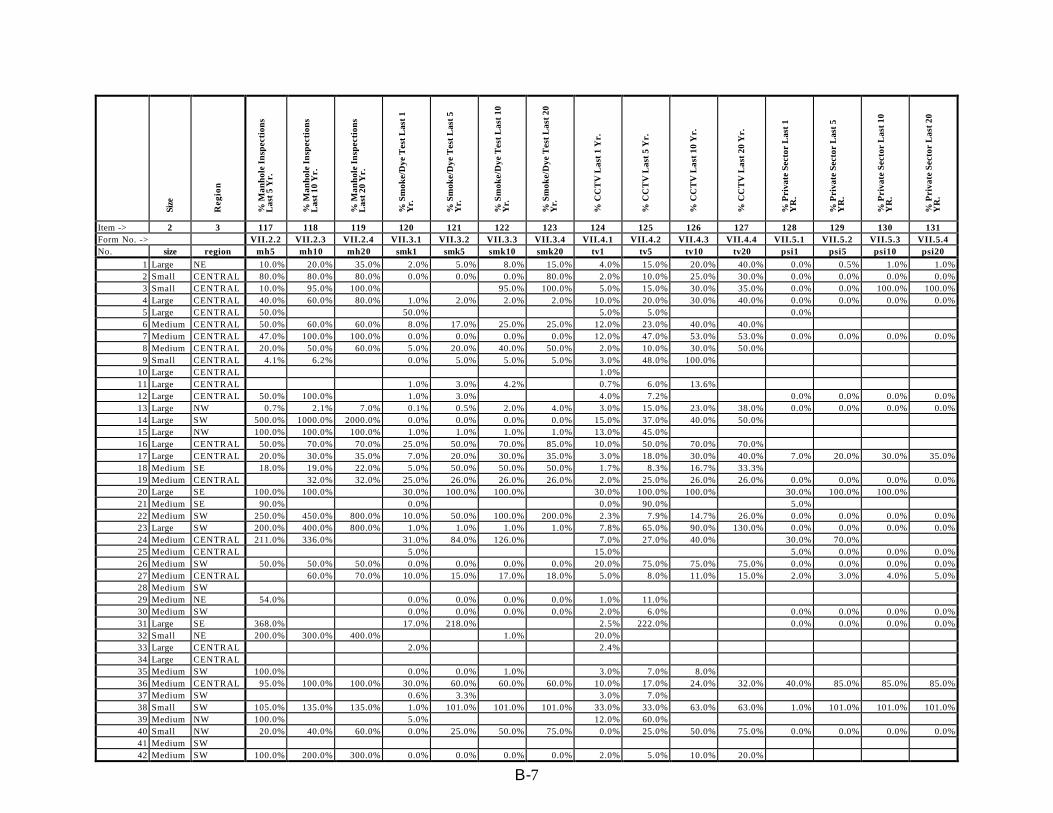
B-7

Size

Reg

ion

% M

anh

ole

Insp

ecti

ons

Las

t 5

Yr.

% M

anh

ole

Insp

ecti

ons

Las

t 10

Yr.

% M

anh

ole

Insp

ecti

ons

Las

t 20

Yr.

% S

mok

e/D

ye T

est

Las

t 1

Yr.

% S

mok

e/D

ye T

est

Las

t 5

Yr.

% S

mok

e/D

ye T

est

Las

t 10

Yr.

% S

mok

e/D

ye T

est

Las

t 20

Yr.

% C

CT

V L

ast

1 Y

r.

% C

CT

V L

ast

5 Y

r.

% C

CT

V L

ast

10 Y

r.

% C

CT

V L

ast

20 Y

r.

% P

riva

te S

ecto

r L

ast

1Y

R.

% P

riva

te S

ecto

r L

ast

5Y

R.

% P

riva

te S

ecto

r L

ast

10Y

R.

% P

riva

te S

ecto

r L

ast

20Y

R.

Item -> 2 3 117 118 119 120 121 122 123 124 125 126 127 128 129 130 131Form No. -> VII.2.2 VII.2.3 VII.2.4 VII.3.1 VII.3.2 VII.3.3 VII.3.4 VII.4.1 VII.4.2 VII.4.3 VII.4.4 VII.5.1 VII.5.2 VII.5.3 VII.5.4No. size region mh5 mh10 mh20 smk1 smk5 smk10 smk20 tv1 tv5 tv10 tv20 psi1 psi5 psi10 psi20

1 Large NE 10.0% 20.0% 35.0% 2.0% 5.0% 8.0% 15.0% 4.0% 15.0% 20.0% 40.0% 0.0% 0.5% 1.0% 1.0%2 Small CENTRAL 80.0% 80.0% 80.0% 0.0% 0.0% 0.0% 80.0% 2.0% 10.0% 25.0% 30.0% 0.0% 0.0% 0.0% 0.0%3 Small CENTRAL 10.0% 95.0% 100.0% 95.0% 100.0% 5.0% 15.0% 30.0% 35.0% 0.0% 0.0% 100.0% 100.0%4 Large CENTRAL 40.0% 60.0% 80.0% 1.0% 2.0% 2.0% 2.0% 10.0% 20.0% 30.0% 40.0% 0.0% 0.0% 0.0% 0.0%5 Large CENTRAL 50.0% 50.0% 5.0% 5.0% 0.0%6 Medium CENTRAL 50.0% 60.0% 60.0% 8.0% 17.0% 25.0% 25.0% 12.0% 23.0% 40.0% 40.0%7 Medium CENTRAL 47.0% 100.0% 100.0% 0.0% 0.0% 0.0% 0.0% 12.0% 47.0% 53.0% 53.0% 0.0% 0.0% 0.0% 0.0%8 Medium CENTRAL 20.0% 50.0% 60.0% 5.0% 20.0% 40.0% 50.0% 2.0% 10.0% 30.0% 50.0%9 Small CENTRAL 4.1% 6.2% 0.0% 5.0% 5.0% 5.0% 3.0% 48.0% 100.0%

10 Large CENTRAL 1.0%11 Large CENTRAL 1.0% 3.0% 4.2% 0.7% 6.0% 13.6%12 Large CENTRAL 50.0% 100.0% 1.0% 3.0% 4.0% 7.2% 0.0% 0.0% 0.0% 0.0%13 Large NW 0.7% 2.1% 7.0% 0.1% 0.5% 2.0% 4.0% 3.0% 15.0% 23.0% 38.0% 0.0% 0.0% 0.0% 0.0%14 Large SW 500.0% 1000.0% 2000.0% 0.0% 0.0% 0.0% 0.0% 15.0% 37.0% 40.0% 50.0%15 Large NW 100.0% 100.0% 100.0% 1.0% 1.0% 1.0% 1.0% 13.0% 45.0%16 Large CENTRAL 50.0% 70.0% 70.0% 25.0% 50.0% 70.0% 85.0% 10.0% 50.0% 70.0% 70.0%17 Large CENTRAL 20.0% 30.0% 35.0% 7.0% 20.0% 30.0% 35.0% 3.0% 18.0% 30.0% 40.0% 7.0% 20.0% 30.0% 35.0%18 Medium SE 18.0% 19.0% 22.0% 5.0% 50.0% 50.0% 50.0% 1.7% 8.3% 16.7% 33.3%19 Medium CENTRAL 32.0% 32.0% 25.0% 26.0% 26.0% 26.0% 2.0% 25.0% 26.0% 26.0% 0.0% 0.0% 0.0% 0.0%20 Large SE 100.0% 100.0% 30.0% 100.0% 100.0% 30.0% 100.0% 100.0% 30.0% 100.0% 100.0%21 Medium SE 90.0% 0.0% 0.0% 90.0% 5.0%22 Medium SW 250.0% 450.0% 800.0% 10.0% 50.0% 100.0% 200.0% 2.3% 7.9% 14.7% 26.0% 0.0% 0.0% 0.0% 0.0%23 Large SW 200.0% 400.0% 800.0% 1.0% 1.0% 1.0% 1.0% 7.8% 65.0% 90.0% 130.0% 0.0% 0.0% 0.0% 0.0%24 Medium CENTRAL 211.0% 336.0% 31.0% 84.0% 126.0% 7.0% 27.0% 40.0% 30.0% 70.0%25 Medium CENTRAL 5.0% 15.0% 5.0% 0.0% 0.0% 0.0%26 Medium SW 50.0% 50.0% 50.0% 0.0% 0.0% 0.0% 0.0% 20.0% 75.0% 75.0% 75.0% 0.0% 0.0% 0.0% 0.0%27 Medium CENTRAL 60.0% 70.0% 10.0% 15.0% 17.0% 18.0% 5.0% 8.0% 11.0% 15.0% 2.0% 3.0% 4.0% 5.0%28 Medium SW29 Medium NE 54.0% 0.0% 0.0% 0.0% 0.0% 1.0% 11.0%30 Medium SW 0.0% 0.0% 0.0% 0.0% 2.0% 6.0% 0.0% 0.0% 0.0% 0.0%31 Large SE 368.0% 17.0% 218.0% 2.5% 222.0% 0.0% 0.0% 0.0% 0.0%32 Small NE 200.0% 300.0% 400.0% 1.0% 20.0%33 Large CENTRAL 2.0% 2.4%34 Large CENTRAL35 Medium SW 100.0% 0.0% 0.0% 1.0% 3.0% 7.0% 8.0%36 Medium CENTRAL 95.0% 100.0% 100.0% 30.0% 60.0% 60.0% 60.0% 10.0% 17.0% 24.0% 32.0% 40.0% 85.0% 85.0% 85.0%37 Medium SW 0.6% 3.3% 3.0% 7.0%38 Small SW 105.0% 135.0% 135.0% 1.0% 101.0% 101.0% 101.0% 33.0% 33.0% 63.0% 63.0% 1.0% 101.0% 101.0% 101.0%39 Medium NW 100.0% 5.0% 12.0% 60.0%40 Small NW 20.0% 40.0% 60.0% 0.0% 25.0% 50.0% 75.0% 0.0% 25.0% 50.0% 75.0% 0.0% 0.0% 0.0% 0.0%41 Medium SW42 Medium SW 100.0% 200.0% 300.0% 0.0% 0.0% 0.0% 0.0% 2.0% 5.0% 10.0% 20.0%

B-8

Size

Reg

ion

Dat

a Q

ual

ity

VII

I

% M

anh

ole

Reh

abed

% M

ain

Lin

e R

ehab

ed

% R

elie

f/ E

qu

al

% P

riva

te S

ecto

r

Dat

a Q

ual

ity

IX

Rel

ief

$ <

197

0

Rel

ief

$ '7

0 -

'79

Rel

ief

$ "

80 -

'89

Rel

ief

$ '9

0 -

96

Rel

ief

$ T

otal

Eq

ual

. $ <

197

0

Eq

ual

. $ '7

0 -

'79

Item -> 2 3 132 133 134 135 136 137 138 139 140 141 142 143 144Form No. -> VIII VIII.1 VIII.2 VIII.3 VIII.4 IX IX.1.1 IX.1.2 IX.1.3 IX.1.4 IX.1.5 IX.2.1 IX.2.2No. size region qual_VIII mhrehab lnrehab rerehab prireh qual_IX rel70 rel79 rel89 rel96 reltot eq70 eq79

1 Large NE 75.0% 50.0% 80.0% 0.0% $0 $0 $0 $48,800,000 $48,800,0002 Small CENTRAL 4 20.0% 50.0% 10.0% 1 $0 $03 Small CENTRAL 3 33.0% 29.0% 62.0% 69.0% 4 $1,000,000 $2,000,000 $5,000,000 $8,000,000 $0 $04 Large CENTRAL 2 90.0% 0.0% 0.0% 0.0% 2 $140,000,000 $72,000,000 $60,000,000 $272,000,000 $0 $05 Large CENTRAL 4 75.0% 75.0% 0.0% 4 $0 $06 Medium CENTRAL 4 20.0% 20.0% 5.0% 0.0% 2 $10,000,000 $10,000,0007 Medium CENTRAL 100.0% 100.0% 100.0% 100.0% 2 $1,303,000 $126,000 $1,216,000 $586,000 $3,231,000 $0 $08 Medium CENTRAL 2 30.0% 40.0% 50.0% 2 $7,000,000 $7,000,0009 Small CENTRAL 3 25.0% 50.0% 1 $0

10 Large CENTRAL $011 Large CENTRAL 4 10.0% 2.0% 1.0% $012 Large CENTRAL $013 Large NW 3 0.1% 1.0% 0.0% 1 $014 Large SW 1 56.0% 56.0% 67.0% 1 $1,400,000 $43,000,000 $44,400,00015 Large NW 2 100.0% 100.0% 100.0% 100.0% 3 $2,500,000 $2,500,00016 Large CENTRAL 4 5.0% 10.0% 5.0% 1 $017 Large CENTRAL 1 40.0% 50.0% 80.0% 90.0% $54,320,000 $54,320,000 $1,025,00018 Medium SE 3 2.0% 2.0% 20.0% 0.0% 4 $20,000,000 $25,000,000 $0 $45,000,000 $0 $019 Medium CENTRAL 40.0% 30.0% 60.0% 0.0% 3 $1,000,000 $2,000,000 $3,000,000 $0 $020 Large SE 1 96.0% 70.0% 25.0% 95.0% $0 $0 $0 $0 $0 $0 $021 Medium SE 2 100.0% 90.0% 2 $0 $022 Medium SW 1 99.9% 100.0% 100.0% 100.0% 2 $18,157,229 $24,570,187 $42,391,582 $85,118,998 $5,000,00023 Large SW 2 1.0% 1.0% 0.0% 0.0% 2 $0 $0 $0 $0 $0 $0 $024 Medium CENTRAL 2 30.0% 30.0% 60.0% 30.0% 2 $9,500,000 $9,500,00025 Medium CENTRAL 4 5.0% 1.0% 1.0% 4 $14,000,000 $14,000,00026 Medium SW 3 0.0% 25.0% 10.0% 0.0% 3 $1,000,000 $5,450,000 $6,450,000 $0 $027 Medium CENTRAL 20.0% 20.0% 10.0% 5.0% 2 $1,100,000 $800,000 $1,200,000 $1,800,000 $4,900,000 $0 $028 Medium SW $029 Medium NE $030 Medium SW 4 5.0% 5.0% 10.0% 0.0% 2 $8,900,000 $4,000,000 $12,900,000 $0 $031 Large SE 2 5.0% 3.0% 50.0% 0.0% 3 $4,000,000 $4,000,00032 Small NE 90.0% 95.0% 3 $900,000 $900,00033 Large CENTRAL 0.0% 3 $25,425,145 $44,638,800 $70,063,94534 Large CENTRAL 40.0% 44.0% 35.0% 17.0% $035 Medium SW 4 25.0% 25.0% 50.0% 3 $2,800,000 $600,000 $3,400,000 $0 $036 Medium CENTRAL 2 20.0% 15.0% 0.0% 0.0% 3 $0 $0 $0 $0 $0 $5,000,00037 Medium SW 3 31.0% $038 Small SW 1 20.0% 2.0% 100.0% 95.0% $039 Medium NW 5.0% 3.0% $040 Small NW 2 5.0% 5.0% 0.0% 3 $0 $0 $0 $2,000,000 $2,000,000 $0 $041 Medium SW 3 99.0% 99.9% 100.0% 100.0% $042 Medium SW 4 95.0% 60.0% 3 $1,500,000 $2,100,000 $3,600,000

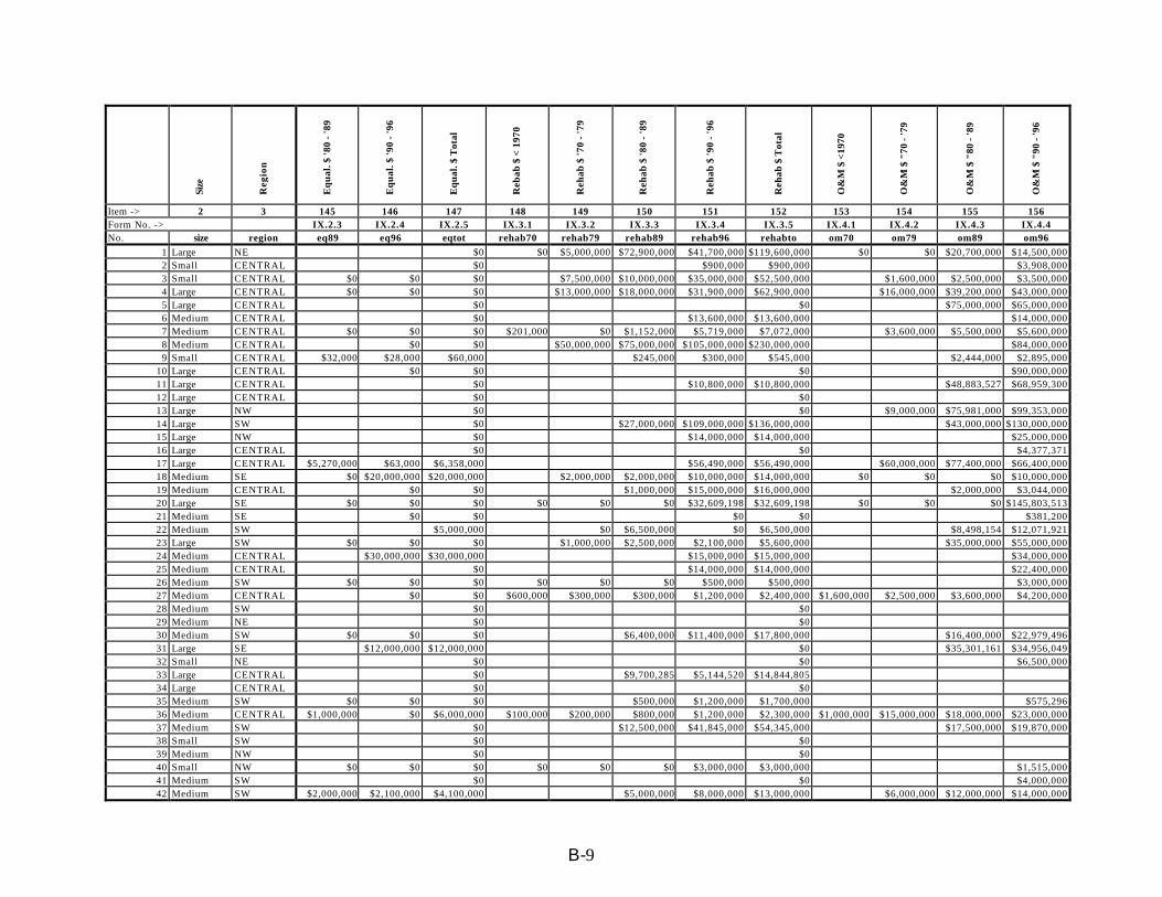
B-9

Size

Reg

ion

Eq

ual

. $ '8

0 -

'89

Eq

ual

. $ '9

0 -

'96

Eq

ual

. $ T

otal

Reb

ab $

< 1

970

Reh

ab $

'70

- '7

9

Reh

ab $

'80

- '8

9

Reh

ab $

'90

- '9

6

Reh

ab $

Tot

al

O&

M $

<19

70

O&

M $

"70

- '7

9

O&

M $

"80

- '8

9

O&

M $

"90

- '9

6

Item -> 2 3 145 146 147 148 149 150 151 152 153 154 155 156Form No. -> IX.2.3 IX.2.4 IX.2.5 IX.3.1 IX.3.2 IX.3.3 IX.3.4 IX.3.5 IX.4.1 IX.4.2 IX.4.3 IX.4.4No. size region eq89 eq96 eqtot rehab70 rehab79 rehab89 rehab96 rehabto om70 om79 om89 om96

1 Large NE $0 $0 $5,000,000 $72,900,000 $41,700,000 $119,600,000 $0 $0 $20,700,000 $14,500,0002 Small CENTRAL $0 $900,000 $900,000 $3,908,0003 Small CENTRAL $0 $0 $0 $7,500,000 $10,000,000 $35,000,000 $52,500,000 $1,600,000 $2,500,000 $3,500,0004 Large CENTRAL $0 $0 $0 $13,000,000 $18,000,000 $31,900,000 $62,900,000 $16,000,000 $39,200,000 $43,000,0005 Large CENTRAL $0 $0 $75,000,000 $65,000,0006 Medium CENTRAL $0 $13,600,000 $13,600,000 $14,000,0007 Medium CENTRAL $0 $0 $0 $201,000 $0 $1,152,000 $5,719,000 $7,072,000 $3,600,000 $5,500,000 $5,600,0008 Medium CENTRAL $0 $0 $50,000,000 $75,000,000 $105,000,000 $230,000,000 $84,000,0009 Small CENTRAL $32,000 $28,000 $60,000 $245,000 $300,000 $545,000 $2,444,000 $2,895,000

10 Large CENTRAL $0 $0 $0 $90,000,00011 Large CENTRAL $0 $10,800,000 $10,800,000 $48,883,527 $68,959,30012 Large CENTRAL $0 $013 Large NW $0 $0 $9,000,000 $75,981,000 $99,353,00014 Large SW $0 $27,000,000 $109,000,000 $136,000,000 $43,000,000 $130,000,00015 Large NW $0 $14,000,000 $14,000,000 $25,000,00016 Large CENTRAL $0 $0 $4,377,37117 Large CENTRAL $5,270,000 $63,000 $6,358,000 $56,490,000 $56,490,000 $60,000,000 $77,400,000 $66,400,00018 Medium SE $0 $20,000,000 $20,000,000 $2,000,000 $2,000,000 $10,000,000 $14,000,000 $0 $0 $0 $10,000,00019 Medium CENTRAL $0 $0 $1,000,000 $15,000,000 $16,000,000 $2,000,000 $3,044,00020 Large SE $0 $0 $0 $0 $0 $0 $32,609,198 $32,609,198 $0 $0 $0 $145,803,51321 Medium SE $0 $0 $0 $0 $381,20022 Medium SW $5,000,000 $0 $6,500,000 $0 $6,500,000 $8,498,154 $12,071,92123 Large SW $0 $0 $0 $1,000,000 $2,500,000 $2,100,000 $5,600,000 $35,000,000 $55,000,00024 Medium CENTRAL $30,000,000 $30,000,000 $15,000,000 $15,000,000 $34,000,00025 Medium CENTRAL $0 $14,000,000 $14,000,000 $22,400,00026 Medium SW $0 $0 $0 $0 $0 $0 $500,000 $500,000 $3,000,00027 Medium CENTRAL $0 $0 $600,000 $300,000 $300,000 $1,200,000 $2,400,000 $1,600,000 $2,500,000 $3,600,000 $4,200,00028 Medium SW $0 $029 Medium NE $0 $030 Medium SW $0 $0 $0 $6,400,000 $11,400,000 $17,800,000 $16,400,000 $22,979,49631 Large SE $12,000,000 $12,000,000 $0 $35,301,161 $34,956,04932 Small NE $0 $0 $6,500,00033 Large CENTRAL $0 $9,700,285 $5,144,520 $14,844,80534 Large CENTRAL $0 $035 Medium SW $0 $0 $0 $500,000 $1,200,000 $1,700,000 $575,29636 Medium CENTRAL $1,000,000 $0 $6,000,000 $100,000 $200,000 $800,000 $1,200,000 $2,300,000 $1,000,000 $15,000,000 $18,000,000 $23,000,00037 Medium SW $0 $12,500,000 $41,845,000 $54,345,000 $17,500,000 $19,870,00038 Small SW $0 $039 Medium NW $0 $040 Small NW $0 $0 $0 $0 $0 $0 $3,000,000 $3,000,000 $1,515,00041 Medium SW $0 $0 $4,000,00042 Medium SW $2,000,000 $2,100,000 $4,100,000 $5,000,000 $8,000,000 $13,000,000 $6,000,000 $12,000,000 $14,000,000

B-10

Size

Reg

ion

O&

M $

Tot

al

Eq

uip

men

t $

< 1

970

Eq

uip

men

t $

'70

- '7

9

Eq

uip

men

t $

'80

- '8

9

Eq

uip

men

t $

'90

- '9

6

Eq

uip

men

t $

Tot

al

Oth

er $

<19

70

Oth

er $

'70

- '7

9

Oth

er $

'80

- '8

9

Oth

er $

'90

- '9

6

Oth

er $

Tot

al

Tot

al $

(al

l yea

rs)

Item -> 2 3 157 158 159 160 161 162 163 164 165 166 167Form No. -> IX.4.5 IX.5.1 IX.5.2 IX.5.3 IX.5.4 IX.5.5 IX.6.1 IX.6.2 IX.6.3 IX.6.4 IX.6.5No. size region omtot omeq70 omeq79 omeq89 omeq96 omeqto oth70 oth79 oth89 oth96 othtot

1 Large NE $35,200,000 $0 $0 $0 $0 $0 $0 $203,600,0002 Small CENTRAL $3,908,000 $0 $0 $4,808,0003 Small CENTRAL $7,600,000 $0 $0 $0 $1,400,000 $1,400,000 $2,214,000 $2,214,000 $71,714,0004 Large CENTRAL $98,200,000 $0 $0 $433,100,0005 Large CENTRAL $140,000,000 $0 $0 $140,000,0006 Medium CENTRAL $14,000,000 $2,800,000 $2,800,000 $0 $40,400,0007 Medium CENTRAL $14,700,000 $0 $0 $0 $0 $0 $0 $25,003,0008 Medium CENTRAL $84,000,000 $7,000,000 $7,000,000 $0 $328,000,0009 Small CENTRAL $5,339,000 $351,650 $351,650 $0 $6,295,650

10 Large CENTRAL $90,000,000 $0 $0 $90,000,00011 Large CENTRAL $117,842,827 $0 $0 $128,642,82712 Large CENTRAL $0 $0 $0 $013 Large NW $184,334,000 $0 $0 $184,334,00014 Large SW $173,000,000 $0 $0 $353,400,00015 Large NW $25,000,000 $0 $18,000,000 $18,000,000 $59,500,00016 Large CENTRAL $4,377,371 $0 $0 $4,377,37117 Large CENTRAL $203,800,000 $0 $0 $320,968,00018 Medium SE $10,000,000 $0 $0 $0 $0 $0 $0 $89,000,00019 Medium CENTRAL $607,000 $1,155,000 $1,762,000 $8,939,900 $8,264,800 $17,204,700 $43,010,70020 Large SE $145,803,513 $0 $0 $0 $0 $0 $0 $0 $0 $126,000 $126,000 $178,538,71121 Medium SE $381,200 $0 $0 $0 $381,20022 Medium SW $20,570,075 $300,000 $1,100,000 $2,150,000 $3,550,000 $0 $120,739,07323 Large SW $90,000,000 $0 $0 $95,600,00024 Medium CENTRAL $34,000,000 $0 $0 $88,500,00025 Medium CENTRAL $22,400,000 $35,000,000 $35,000,000 $0 $85,400,00026 Medium SW $3,000,000 $150,000 $150,000 $0 $10,100,00027 Medium CENTRAL $0 $0 $19,200,00028 Medium SW $0 $0 $0 $029 Medium NE $0 $0 $0 $030 Medium SW $39,379,496 $1,700,000 $645,135 $2,345,135 $0 $72,424,63131 Large SE $70,257,210 $1,651,887 $1,651,887 $0 $87,909,09732 Small NE $6,500,000 $0 $0 $7,400,00033 Large CENTRAL $0 $0 $0 $84,908,75034 Large CENTRAL $0 $0 $035 Medium SW $575,296 $0 $0 $0 $0 $5,675,29636 Medium CENTRAL $66,000,000 $0 $0 $74,300,00037 Medium SW $37,370,000 $0 $0 $91,715,00038 Small SW $0 $0 $0 $039 Medium NW $0 $0 $0 $040 Small NW $1,515,000 $0 $0 $0 $0 $0 $0 $6,515,00041 Medium SW $4,000,000 $0 $0 $4,000,00042 Medium SW $32,000,000 $0 $0 $52,700,000

B-11

Size

Reg

ion

Per

f. W

eigh

t -

Pip

e F

ailu

re

Per

f. W

eigh

t - S

SOs

Per

f. W

eigh

t -

Com

pla

ints

Per

f. W

eigh

t -

PS

Fai

lure

s

Per

f. W

eigh

t - P

k H

r/ A

DF

Per

f. W

eigh

t - P

k M

o/ A

DF

Per

f. W

eigh

t -

Tot

al

Mai

nt.

Wei

ght

- %

Cle

aned

Mai

nt.

Wei

ght

- %

Roo

tC

lean

ed

Mai

nt.

Wei

ght

- L

ift

Sta

tion

Ser

vice

Mai

nt.

Wei

ght

-F

low

/Cap

acit

y

Mai

nt.

Wei

ght

- M

anh

ole

Mai

nt.

Wei

ght

- S

mok

e

Mai

nt.

Wei

ght

- C

CT

V

Mai

nt.

Wei

ght -

Pri

vate

Item -> 2 3 168 169 170 171 172 173 174 175 176 177 178 179 180 181 182Form No. -> X.1.1 X.1.2 X.1.3 X.1.4 X.1.5 X.1.6 X.1.7 X.2.1 X.2.2 X.2.3 X.2.4 X.2.5 X.2.6 X.2.7 X.2.8No. size region perpf perfsso perfcomp perfps perfpkhr perfpkmo perktot maintcl maintrt maintls maintfm maintmh maintsmk mainttv maintpri

1 Large NE2 Small CENTRAL 27.0% 32.0% 32.0% 9.0% 0.0% 0.0% 100% 25.0% 10.0% 5.0% 1.0% 1.0% 1.0% 10.0% 5.0%3 Small CENTRAL 35.0% 35.0% 20.0% 0.0% 5.0% 5.0% 100% 15.0% 0.0% 5.0% 5.0% 2.0% 3.0% 0.0%4 Large CENTRAL 25.0% 25.0% 25.0% 25.0% 100% 6.0% 0.0% 35.0% 18.0% 12.0% 0.0% 13.0% 0.0%5 Large CENTRAL 18.0% 18.0% 14.0% 27.0% 14.0% 9.0% 100% 15.0% 15.0% 15.0% 8.0% 5.0% 5.0% 10.0% 3.0%6 Medium CENTRAL 25.0% 25.0% 40.0% 10.0% 0.0% 0.0% 100% 10.0% 10.0% 10.0%7 Medium CENTRAL 16.7% 25.0% 25.0% 16.7% 16.6% 0.0% 100% 10.0% 0.0% 10.0% 20.0% 10.0% 0.0% 10.0% 0.0%8 Medium CENTRAL 80.0% 5.0% 10.0% 5.0% 100%9 Small CENTRAL 35.0% 15.0% 20.0% 20.0% 7.0% 3.0% 100% 40.0% 5.0% 20.0% 15.0%

10 Large CENTRAL 20.0% 20.0% 40.0% 10.0% 5.0% 5.0% 100% 20.0% 10.0% 0.0% 5.0% 4.0% 10.0% 20.0% 10.0%11 Large CENTRAL 15.0% 30.0% 30.0% 15.0% 5.0% 5.0% 100% 12.0% 10.0% 10.0% 4.0% 8.0% 6.0% 12.0% 4.0%12 Large CENTRAL 22.0% 10.0% 22.0% 2.0% 3.0% 2.0% 10.0% 1.0%13 Large NW 5.0% 30.0% 30.0% 35.0% 0.0% 0.0% 100% 25.0% 5.0% 35.0% 10.0% 5.0% 0.0% 10.0% 0.0%14 Large SW 25.0% 25.0% 15.0% 25.0% 8.0% 2.0% 100% 15.0% 15.0% 15.0% 5.0% 5.0% 10.0%15 Large NW 80.0% 5.0% 10.0% 2.0% 2.0% 1.0% 100% 60.0% 5.0% 5.0% 5.0% 1.0% 1.0% 12.0% 3.0%16 Large CENTRAL 20.0% 20.0% 20.0% 20.0% 10.0% 10.0% 100% 13.6% 9.1% 31.9% 0.9% 2.7% 0.9%17 Large CENTRAL 25.0% 39.0% 25.0% 3.0% 5.0% 3.0% 100% 15.0% 12.0% 2.0% 10.0% 10.0% 2.0% 10.0% 2.0%18 Medium SE 20.0% 20.0% 20.0% 20.0% 5.0% 15.0% 100% 4.8% 19.0% 9.5% 9.5% 4.8% 9.5% 4.8% 4.8%19 Medium CENTRAL 20.0% 10.0% 20.0% 15.0% 15.0% 100% 8.0% 5.0% 20.0% 15.0% 5.0% 5.0% 5.0% 1.0%20 Large SE 20.0% 20.0% 10.0% 10.0% 20.0% 20.0% 100% 5.0% 5.0% 5.0% 10.0% 10.0% 10.0% 10.0% 10.0%21 Medium SE 30.0% 25.0% 10.0% 25.0% 0.0% 10.0% 100% 20.0% 0.0% 50.0% 0.0% 5.0% 0.0% 15.0% 0.0%22 Medium SW 12.0% 40.0% 20.0% 25.0% 2.0% 1.0% 100% 34.0% 1.0% 20.0% 10.0% 9.0% 1.0% 15.0% 0.0%23 Large SW 50.0% 10.0% 20.0% 20.0% 0.0% 0.0% 100% 35.0% 0.0% 15.0% 0.0% 20.0% 3.0% 15.0% 0.0%24 Medium CENTRAL 15.0% 10.0% 20.0% 50.0% 2.0% 3.0% 100% 0.0% 30.0% 10.0% 2.0% 2.0% 2.0% 7.0% 1.0%25 Medium CENTRAL 30.0% 30.0% 20.0% 10.0% 5.0% 5.0% 100%26 Medium SW 10.0% 25.0% 25.0% 20.0% 10.0% 10.0% 100% 10.0% 10.0% 10.0% 20.0% 10.0% 0.0% 10.0% 0.0%27 Medium CENTRAL 30.0% 20.0% 10.0% 10.0% 10.0% 100% 10.0% 10.0% 10.0% 6.0% 15.0% 6.0% 6.0% 3.0%28 Medium SW29 Medium NE30 Medium SW 10.0% 20.0% 60.0% 10.0% 0.0% 0.0% 100% 20.0% 15.0% 5.0% 10.0% 5.0% 0.0% 8.0% 1.0%31 Large SE 15.0% 25.0% 25.0% 25.0% 5.0% 5.0% 100% 20.0% 20.0% 30.0% 1.0% 1.0% 2.0% 4.0% 0.0%32 Small NE 5.0% 20.0% 5.0% 70.0% 0.0% 0.0% 100% 15.0% 0.0% 30.0% 5.0% 20.0% 0.0% 25.0%33 Large CENTRAL 22.0% 27.0% 20.0% 20.0% 8.0% 3.0% 100% 13.0% 8.0% 11.0% 7.0% 7.0% 5.0% 5.0% 2.0%34 Large CENTRAL 25.0% 35.0% 15.0% 3.0% 2.0% 100%35 Medium SW 20.0% 20.0% 10.0% 25.0% 13.0% 12.0% 100% 12.0% 5.0% 14.0% 10.0% 7.0% 5.0% 14.0% 5.0%36 Medium CENTRAL 15.0% 20.0% 30.0% 5.0% 20.0% 10.0% 100% 5.0% 5.0% 5.0% 5.0% 10.0% 10.0% 10.0% 5.0%37 Medium SW 30.0% 40.0% 10.0% 20.0% 100% 27.0% 17.0% 3.0% 4.0% 2.0% 7.0% 14.0% 0.0%38 Small SW 12.0% 48.0% 20.0% 15.0% 1.0% 4.0% 100% 18.0% 10.0% 17.0% 6.0% 4.0% 5.0% 10.0% 3.0%39 Medium NW 10.0% 20.0% 30.0% 5.0% 25.0% 10.0% 100% 30.0% 2.0% 12.0% 2.0% 2.0% 1.0% 12.0% 1.0%40 Small NW 20.0% 25.0% 20.0% 15.0% 10.0% 10.0% 100% 20.0% 10.0% 15.0% 5.0% 10.0% 5.0% 10.0% 0.0%41 Medium SW 25.0% 15.0% 15.0% 25.0% 10.0% 10.0% 100% 50.0% 20.0% 13.0% 1.0% 1.0% 4.0% 5.0% 1.0%42 Medium SW 10.0% 50.0% 10.0% 20.0% 5.0% 5.0% 100% 10.0% 10.0% 10.0% 20.0% 5.0% 0.0% 40.0% 0.0%

B-12

Size

Reg

ion

Mai

nt.

Wei

ght

- M

anh

ole

Reh

ab

Mai

nt.

Wei

ght

- M

ain

Reh

ab

Mai

nt.

Wei

ght

- R

elie

f

Mai

nt.

Wei

ght -

Pri

vate

I/I

Mai

nt.

Wei

ght

- T

otal

Sat

isfa

ctio

n

Wh

at D

iffe

ren

t

Item -> 2 3 183 184 185 186 187 188 189Form No. -> X.2.9 X.2.10 X.2.11 X.2.12 X.1 X.2No. size region maintmhr maintmn maintre maintpr maintot satis diff

1 Large NE2 Small CENTRAL 1.0% 35.0% 5.0% 1.0% 100.0% b3 Small CENTRAL 5.0% 35.0% 15.0% 15.0% 100.0% b4 Large CENTRAL 8.0% 8.0% 0.0% 0.0% 100.0% a5 Large CENTRAL 5.0% 5.0% 4.0% 10.0% 100.0% c6 Medium CENTRAL 10.0% 10.0% 10.0% 40.0% 100.0% c7 Medium CENTRAL 0.0% 20.0% 10.0% 10.0% 100.0% b8 Medium CENTRAL 10.0% 70.0% 20.0% 0.0% 100.0% b9 Small CENTRAL 10.0% 10.0% 100.0% c

10 Large CENTRAL 1.0% 5.0% 5.0% 10.0% 100.0% b11 Large CENTRAL 10.0% 12.0% 6.0% 6.0% 100.0% c12 Large CENTRAL 8.0% 10.0% 5.0% 5.0% 100.0%13 Large NW 5.0% 5.0% 0.0% 0.0% 100.0% b14 Large SW 5.0% 15.0% 15.0% 100.0% a15 Large NW 1.0% 4.0% 2.0% 1.0% 100.0% b16 Large CENTRAL 4.5% 27.3% 9.1% 100.0% d17 Large CENTRAL 10.0% 10.0% 10.0% 7.0% 100.0% b18 Medium SE 9.5% 14.2% 4.8% 4.8% 100.0% c19 Medium CENTRAL 20.0% 2.0% 4.0% 100.0% c20 Large SE 5.0% 10.0% 10.0% 10.0% 100.0% a21 Medium SE 5.0% 5.0% 0.0% 0.0% 100.0% c22 Medium SW 2.0% 2.0% 5.0% 1.0% 100.0% a23 Large SW 2.0% 10.0% 0.0% 0.0% 100.0% b24 Medium CENTRAL 4.0% 10.0% 2.0% 30.0% 100.0% b25 Medium CENTRAL c&d26 Medium SW 10.0% 10.0% 10.0% 0.0% 100.0% b27 Medium CENTRAL 11.0% 6.0% 2.0% 100.0% d28 Medium SW b29 Medium NE30 Medium SW 5.0% 10.0% 20.0% 1.0% 100.0% b31 Large SE 1.0% 5.0% 15.0% 1.0% 100.0% d32 Small NE 5.0% 0.0% 100.0% b33 Large CENTRAL 6.0% 13.0% 18.0% 5.0% 100.0% d34 Large CENTRAL35 Medium SW 8.0% 8.0% 7.0% 5.0% 100.0% d36 Medium CENTRAL 15.0% 10.0% 5.0% 15.0% 100.0% c37 Medium SW 1.0% 20.0% 5.0% 0.0% 100.0% d38 Small SW 5.0% 10.0% 2.0% 10.0% 100.0% b39 Medium NW 4.0% 12.0% 12.0% 10.0% 100.0% b40 Small NW 10.0% 10.0% 0.0% 5.0% 100.0% c41 Medium SW 1.0% 2.0% 1.0% 1.0% 100.0% b42 Medium SW 0.0% 5.0% 0.0% 0.0% 100.0% c

Appendix C

Maintenance Activities Weighting

C-1

Collection System Maintenance Weighting

Maintenance Weighting - % System Cleaned

Crosstab Table For Average maintcl by region and size

Large Medium Small Avg- Reg. Avg - AllCENTRAL 13.0% 5.4% 26.7% 15.0%NE 0.0% 0.0% 15.0% 5.0%NW 42.5% 30.0% 20.0% 30.8%SE 12.5% 12.4% 12.5%SW 25.0% 20.4% 18.0% 21.1%

18.6% 13.6% 19.9% 16.9% 17.7%Count-> 36

Maintenance Weighting - % System Root CleanedCrosstab Table For Average maintrt by region and size


6.6% 5.8% 6.3% 6.5% 8.4%Count-> 36

Maintenance Weighting - Lift Station ServiceCrosstab Table For Average maintls by region and size


13.3% 11.9% 18.0% 14.8% 14.2%Count-> 36

Maintenance Weighting - Flow MonitoringCrosstab Table For Average maintfm by region and size


4.3% 4.4% 4.5% 4.5% 6.9%Count-> 33

C-2

Maintenance Weighing - Manhole InspectionCrosstab Table For Average maintmh by region and size


5.3% 3.4% 10.0% 5.9% 6.5%Count-> 35

Maintenance Weighing - Smoke TestingCrosstab Table For Average maintsmk by region and size


2.3% 2.2% 2.6% 2.5% 3.3%Count-> 31

Maintenance Weighting - CCTVCrosstab Table For Average mainttv by region and size


7.9% 8.0% 12.3% 9.2% 10.5%Count-> 34

Maintenance Weighting - Private Sector InspectionsCrosstab Table For Average maintpri by region and size


1.8% 1.1% 1.2% 1.5% 2.0%Count-> 32

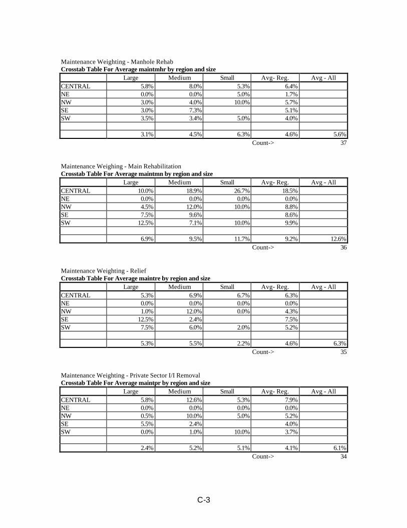
C-3

Maintenance Weighting - Manhole RehabCrosstab Table For Average maintmhr by region and size


3.1% 4.5% 6.3% 4.6% 5.6%Count-> 37

Maintenance Weighing - Main RehabilitationCrosstab Table For Average maintmn by region and size


6.9% 9.5% 11.7% 9.2% 12.6%Count-> 36

Maintenance Weighting - ReliefCrosstab Table For Average maintre by region and size


5.3% 5.5% 2.2% 4.6% 6.3%Count-> 35

Maintenance Weighting - Private Sector I/I RemovalCrosstab Table For Average maintpr by region and size


2.4% 5.2% 5.1% 4.1% 6.1%Count-> 34

Appendix D

Collection System Performance Weighting

D-1

Collection System Performance WeightingPerformance Weighting - Pipe FailureCrosstab Table For Average perpf by region and size


23.2% 15.5% 17.3% 18.9% 23.3%count-> 38

Performance Weighting - SSOCrosstab Table For Average perfsso by region and size


16.0% 17.9% 30.1% 20.8% 24.4%count-> 38

Performance Weighting - ComplaintsCrosstab Table For Average perfcomp by region and size


15.6% 17.1% 17.3% 16.6% 21.4%count-> 38

Performance Weighting - Pump Station FailureCrosstab Table For Average perfps by region and size


14.7% 12.3% 27.4% 17.6% 18.3%count-> 38

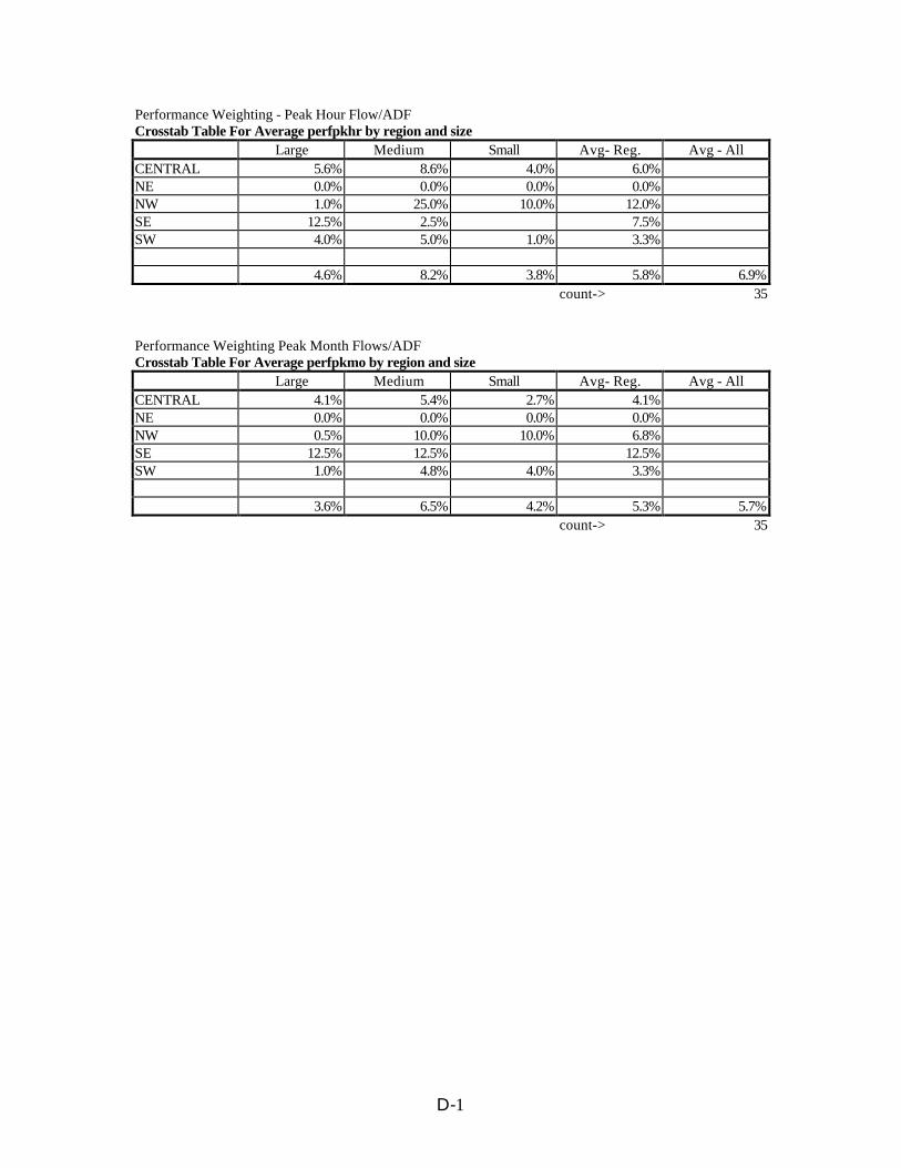
D-1

Performance Weighting - Peak Hour Flow/ADFCrosstab Table For Average perfpkhr by region and size


4.6% 8.2% 3.8% 5.8% 6.9%count-> 35

Performance Weighting Peak Month Flows/ADFCrosstab Table For Average perfpkmo by region and size


3.6% 6.5% 4.2% 5.3% 5.7%count-> 35

Appendix E

Literature Review

FINAL.DOC E-3

Appendix E Literature Review

Review of the Literature

The authors of this project conducted an extensive literature search to obtain nationwide

information on current trends in maintenance of wastewater collection systems.

The literature review included a search of the 1990-1997 publications listed below:

$ Beton werk und Fertigtel - Technik$ Civil Engineering$ Engineering News Record$ Journal of Infrastructure System$ Journal of Professional Issues in Engineering$ Journal of Urban Planning and Development$ Optimizing the Resources for Water Management - Proceedings of the ASCE 17th

Annual National Conference (1990)$ Proceedings of the International Conference on Pipeline Infrastructure II (1993)$ Proceedings of the 1995 Construction Congress$ Proceedings of the 1991 Specialty Conference on Environmental Engineering$ Public Works$ Urban Drainage Rehabilitation Programs and Techniques (1994)$ Water Engineering and Management$ Water Resources Infrastructure: Needs, Economic, and Financing (1990)$ Water Resources Planning and Management and Urban Water Resources (1991) -

Proceedings of the 18th Annual Conference and Symposium$ Water Resources Planning and Management and Urban Water Resources (1993) -

Proceedings of the 20th Anniversary Conference on Water Management in the�90s

$ Water Resources Planning and Management: Saving a Threatened Resource - InSearch of Solutions, Proceedings of the Water Resources Sessions at WaterForum (1992)

$ 1992 Nation Conference on Water Resources Planning and Management (WaterForum �92)

FINAL.DOC E-4

Summary of Findings

Information from the following papers was used, in part, in the development of the survey

form used for this study.

Anonymous (1994) Districts expand sewer rehabilitation program. Public Works, v125,

n 9, 34-35.

The article describes system reinvestment through installation of a pipe liner in 40,000 linear

feet of large diameter sewer (48 inches and larger) in 1993. The systems oldest sewers

were constructed in 1926.

Burgess, Edward H. (1990) Planning model for sewer system rehabilitation. Proceedings

of ASCE's Conference on Water Resources Infrastructure: Needs, Economics, and

Financing, Fort Worth, TX, April 18-20, 1990.

A probabilistic model is developed to simulate long-term variation in the structural condition

of wastewater collection systems. The effect of both deterioration and rehabilitation

strategies as an extension of current sewer system planning and management practices was

discussed.

Bergman, William (1991) 1991 Update on sanitary sewer rehabilitation metropolitan

Chicago. Water Resources Planning and Management and Urban Water Resources, 825-

829.

The following data for the Metropolitan Water Reclamation District of Greater Chicago

(MWRDGC) was reported:

$ Provided collection for 875 square miles, 5,100,000 people plus commercial/industrialpopulation equivalent to 4,500,000 people.

$ 520 miles of interceptor sewer, seven water reclamation plants.$ 125 communities own and operate separate sanitary sewers with a total discharge

population equivalent of 2,000,000 people.$ MWRDGC required each community to do comprehensive sewer rehabilitation in

1973.$ 1973-1985 - $100,000,000 was spent by tributary communities, but was not

successful in reducing I/I.$ 1986 - I/I Corrective Action Program (ICAP).$ 1987-1991 - estimated that an additional $140,000,000 (to the previous

$100,000,000) would be needed to complete cost-effective rehabilitation.

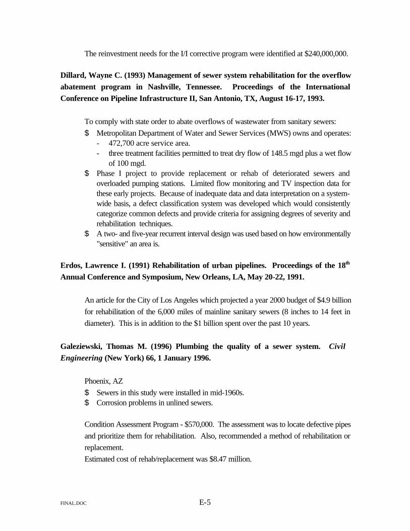
FINAL.DOC E-5

The reinvestment needs for the I/I corrective program were identified at $240,000,000.

Dillard, Wayne C. (1993) Management of sewer system rehabilitation for the overflow

abatement program in Nashville, Tennessee. Proceedings of the International

Conference on Pipeline Infrastructure II, San Antonio, TX, August 16-17, 1993.

To comply with state order to abate overflows of wastewater from sanitary sewers:

$ Metropolitan Department of Water and Sewer Services (MWS) owns and operates:- 472,700 acre service area.- three treatment facilities permitted to treat dry flow of 148.5 mgd plus a wet flow

of 100 mgd.$ Phase I project to provide replacement or rehab of deteriorated sewers and

overloaded pumping stations. Limited flow monitoring and TV inspection data forthese early projects. Because of inadequate data and data interpretation on a system-wide basis, a defect classification system was developed which would consistentlycategorize common defects and provide criteria for assigning degrees of severity andrehabilitation techniques.

$ A two- and five-year recurrent interval design was used based on how environmentally"sensitive" an area is.

Erdos, Lawrence I. (1991) Rehabilitation of urban pipelines. Proceedings of the 18th

Annual Conference and Symposium, New Orleans, LA, May 20-22, 1991.

An article for the City of Los Angeles which projected a year 2000 budget of $4.9 billion

for rehabilitation of the 6,000 miles of mainline sanitary sewers (8 inches to 14 feet in

diameter). This is in addition to the $1 billion spent over the past 10 years.

Galeziewski, Thomas M. (1996) Plumbing the quality of a sewer system. Civil Engineering (New York) 66, 1 January 1996.

Phoenix, AZ

$ Sewers in this study were installed in mid-1960s.$ Corrosion problems in unlined sewers.

Condition Assessment Program - $570,000. The assessment was to locate defective pipes

and prioritize them for rehabilitation. Also, recommended a method of rehabilitation or

replacement.

Estimated cost of rehab/replacement was $8.47 million.

FINAL.DOC E-6

Phoenix wastewater collection system size:

$ 3,700 miles (8 to 90-inch in diameter).$ 7,200 manholes.

Unlined pipe: 116,347 ft (24 to 60-inch diameter) 258 manholes.

Gray, William R. (1990) Sanitary sewer bypass reduction program. Water/Engineeringand Management, v 137, n 5, May 1990.

Elmhurst, Illinois, has a population of 44,000. The area is served by approximately 77,000

linear feet of gravity sewer and 10 lift stations.

Elmhurst implemented a program to reduce the incidence of sanitary sewer backups into

basements and bypassing of wastewater into receiving streams following moderate to

intense storm events.

Upgrading of system included 59,000 linear feet of sanitary relief sewers and force mains

along with upgrading of lift stations.

Gregory, Henry N. Jr. (1990) New technologies help Houston inspect its sewers. PublicWorks, v 121, n 2, February 1990.

The City of Houston, Texas, conducted a physical inspection program on its 4,500 mile

sewer system using laptop computers and image storage software and hardware. Cost of

the program was estimated at $100 million.

Harman, Duane G. (1990) Evaluation plus history equals sewer renovation. Proceedings

of ASCE's Conference on Water Resources Infrastructure: Needs, Economics, and

Financing, Fort Worth, TX, April 18-20, 1990.

Fort Worth Zoo

477 manholes, 194,000 feet of sewer

3,952 residential units and 18 acres of commercial.

Intensive survey activities including flow monitoring, computer modeling, and analysis for

cost-effective I/I removal. Key data are as follows:

$ 2060 I/I sources identified (849 infiltration sources, 1,211 inflow sources).$ The I/I costs are for treatment and transport of the I/I flow rate. Treatment cost is for

increasing treatment capacity, plus the present worth of increased cost of plant

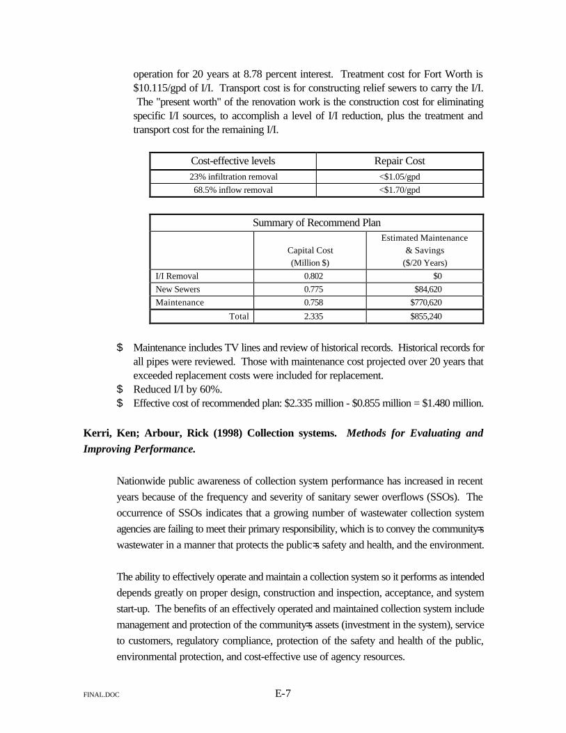
FINAL.DOC E-7

operation for 20 years at 8.78 percent interest. Treatment cost for Fort Worth is$10.115/gpd of I/I. Transport cost is for constructing relief sewers to carry the I/I. The "present worth" of the renovation work is the construction cost for eliminatingspecific I/I sources, to accomplish a level of I/I reduction, plus the treatment andtransport cost for the remaining I/I.

Cost-effective levels Repair Cost

23% infiltration removal <$1.05/gpd

68.5% inflow removal <$1.70/gpd

Summary of Recommend Plan

Capital Cost

(Million $)

Estimated Maintenance

& Savings

($/20 Years)

I/I Removal 0.802 $0

New Sewers 0.775 $84,620

Maintenance 0.758 $770,620

Total 2.335 $855,240

$ Maintenance includes TV lines and review of historical records. Historical records forall pipes were reviewed. Those with maintenance cost projected over 20 years thatexceeded replacement costs were included for replacement.

$ Reduced I/I by 60%.$ Effective cost of recommended plan: $2.335 million - $0.855 million = $1.480 million.

Kerri, Ken; Arbour, Rick (1998) Collection systems. Methods for Evaluating andImproving Performance.

Nationwide public awareness of collection system performance has increased in recent

years because of the frequency and severity of sanitary sewer overflows (SSOs). The

occurrence of SSOs indicates that a growing number of wastewater collection system

agencies are failing to meet their primary responsibility, which is to convey the community=s

wastewater in a manner that protects the public=s safety and health, and the environment.

The ability to effectively operate and maintain a collection system so it performs as intended

depends greatly on proper design, construction and inspection, acceptance, and system

start-up. The benefits of an effectively operated and maintained collection system include

management and protection of the community=s assets (investment in the system), service

to customers, regulatory compliance, protection of the safety and health of the public,

environmental protection, and cost-effective use of agency resources.

FINAL.DOC E-8

This manual includes:

$ Information on how to establish an effective collection system O&M program that willmaintain the functional and structural integrity of the collection system,

$ Information regarding how to evaluate the adequacy and effectiveness of existing O&Mprograms through the use of performance indicators, and

$ Information on how to improve the performance of collection systems.

Steps in the evaluation process include:

$ Verifying and validating what is being done right,

$ Identifying areas of the O&M program that affect system performance,

$ Identifying areas of opportunity for more cost-effective O&M of the system,

$ Identifying areas of potential liability, and

$ Adapting successful ideas and solutions from other agencies nationwide to improveperformance.

This manual provides a detailed analysis of the data provided by 13 agencies whose

systems consist of sanitary sewers only. The benchmark data are organized by both

population served and miles of gravity sewer. Agencies can compare their system

characteristics with other systems and also their level of production, performance, and

budget with other similar agencies. Subjects for comparison include operation and

maintenance data, finance, training and certification, safety, level of service, regulatory

compliance, O&M policies and procedures, and information management. Critical

performance indicators include stoppages per 100 miles of gravity sewer, complaints per

100,000 population served, and response time for service requests

.

Macaitis, William (1993) Collection system inspection and rehabilitation program. WaterResources Planning and Management and Urban Water Resources.

Metropolitan Water Reclamation District of Greater Chicago:

$ Serves area of 875 square miles.$ 535 mile collection system.$ The first sewer was constructed in 1906. Present worth of sewers is $3.8

billion. Sewers 50 years or older have a total length of 170 miles and a present worthof $1.5 billion.

$ Spent approximately $3 million in last 10 years on emergency repairs.

FINAL.DOC E-9

Macaitis, William; Kuhl, Robert (1994) Local Sewer Rehabilitation - Metro Chicago.

Urban Drainage Rehabilitation Programs and Techniques, 111-122

The Metropolitan Water Reclamation District of Greater Chicago is a regional wastewater

agency encompassing an area of 875 sq. miles in Cook County, Illinois. The city of

Chicago and 124 neighboring municipalities are served by the Water Reclamation District.

The purpose of the study was to reduce overloading of the conveyance system and to

alleviate the widespread occurrence of home and basement flooding.

The Water Reclamation District formulated and adopted a rehabilitation program in the

1970s and revised the program in 1985, which was patterned after the US EPA cost-

effective methodology. The agencies were given two options: Either reduce the average

wet-weather flow to 150 gpcpd under the old (1970s) program or implement a sewer

rehabilitation program based upon the US EPA Corrective Action Program

(ICAP). Details of the ICAP option were defined in the "Sewer Summit Agreement,"

developed jointly by the IEPA, the Water Reclamation District, and local agencies.

The main features of the ICAP program included a Sewer System Evaluation Study

(SSES) which consisted of a data collection and flow monitoring program, sewer system

investigations, plans for corrective action in both public and private sectors, and

construction of projects.

Based on the submitted SSES reports, the Water Reclamation District estimated that the

total cost for local sanitary sewer systems rehabilitation would be $240 million (1985

dollars). Of this total, $100 million of work was completed prior to the 1985 Sewer

Summit Agreement. The ICAP program represents a savings of $1.16 billion to the local

agencies compared to the estimated $1.4 billion needed to complete the Sewer

Rehabilitation, 150 option program. As a result of a 1993 Water Reclamation District

survey, with 90 percent of the public sector and 80 percent of the private sector work

completed, a revised estimate of $195 million (from the original $240 million estimate) was

projected to be spent by the local agencies on sanitary sewer system rehabilitation as a

result of the Sewer Summit Agreement.

Of the corrective work performed in the public sector, all identified I/I sources associated

with manholes were found to be cost-effective to repair. In general, sewer grouting was

determined to be a cost-effective repair. Sewer lining, sewer replacement, and

interconnection repairs were usually found not to be cost-effective. In the private sector,

FINAL.DOC E-10

down spouts and foundation sumps were found to be cost-effective repair items. Gravity

foundation drain disconnections were generally found not to be cost-effective.

All agencies are required by the Sewer Summit Agreement to establish a long-term

Operation & Maintenance (O&M) program. The three core elements of an acceptable

O&M program are:

1. A five-year inspection cycle of all sewers and appurtenances.

2. TV inspection of any problem areas.

3. A program funded by annual budget appropriations or user fees.

The Water Reclamation District's treatment plants and interceptor system were designed

and sized nominally for 150 gpcpd. The ICAP program reduced flows from 764 to 370

gpcpd, but the residual flow would have to be accommodated to prevent backups and

overflows. It was determined that storing peak flows at remote sites for treatment at off-

peak hours and providing additional regional treatment plant capacity as required would

be the most cost-effective plan. The flow equalization was estimated to cost $0.6 billion.

Macaitis, William; Paintal, Amreek (1994) Interceptor inspection and rehabilitation

program. Urban Drainage Rehabilitation Programs and Techniques, 123-142.

Description of methods conducted in inspection and rehabilitation for program: physical

inspection, CCTV inspection, void defect inspection, flow monitoring, computerized

mapping, documentation, and underground advisory committee.

Metropolitan Water Reclamation District of Greater Chicago: One third of the system is

more than 50 years old; with cave-ins being a common occurrence.

$ Based on costs experienced during last 10 years, average annual cost of unscheduledemergency repair has been $300,000.

$ A program cost $1.4 million per year not including cost of rehabilitating sewers

Nelson, Richard E., AASSES Experience in Kansas,@@ presented at the Kansas Water

Pollution Control Association, Lawrence, KS, April 1993, 20 pages.

Sewer System Evaluation Survey (SSES) are being performed or being considered

throughout Kansas in an effort to meet regulator requirements and to improve sewerage

service to customers. Following completion of the SSES, rehabilitation work is performed

to correct identified deficiencies. A survey was conducted encompassing 10 cities and

agencies, which include 12 service areas. The cities/agencies surveyed ranged in area from

9 to 150 square miles, with 55 to 1,500 miles of sewer line and an average daily flow

FINAL.DOC E-11

(ADF) from 1.2 MGD to 60 MGD, with populations ranging from 10,500 to 285,000

persons. The average age of the cities/agencies ranged from 20 to 63 years. Conclusions

based on collected information include: (1) routine inspection activities include manhole

inspections, line inspections and testing, and private sector work, (2) sewer systems

degrade continuously and a plan is required to effectively manage this degradation, (3)

rehabilitation is effective in improving system performance, (4) rehabilitation costs are

typically about $25 per foot of sewer, but vary widely and are system-dependent, and (5)

annual inspection frequency of about 6 to 10 percent of the system per year can be a cost-

effective way to manage system performance.

Malik, Omesh; Pumphery, Jr., Norman D.; Roberts, Freddy L., AASanitary Sewers: State-

of-the-Practice@@ . ASCE Infrastructure condition Assessment, 297-306.

Researchers are developing the framework of a sanitary sewer management system

(SSMS). Too often and predominantly, a Aworst first@ or Acrisis management@ system

exists, causing inefficient use of the meager resources available for maintaining and

upgrading the sanitary sewer system. Of those who have a systematic management

procedure in place, little compatibility exists so that the municipalities have difficulty in

sharing information. As a first step in development of the SSMS, a state-of-practice survey

was mailed to over 450 cities and sanitation districts across the United States. A survey

was conducted through 121 cities and agencies, with population ranging from 40,000 to

832,750 persons. Cities with populations less than 20,000 or with less than 50 miles of

sewer have been excluded from this study. The average age of the cities/agencies ranged

from 29 to 42 years. An average city or sanitation district has 1,075 kilometers (667 miles)

of sewer, a population of 221,199, and an annual budget of almost $3 million. On the

average each city spent an average of about $14 per person and $2,790 per kilometer

($4,497 per mile) of sewer in the 1995. Each kilometer of sewer serves 228 people.

According the survey, only 48% of the cities have some established procedures set down

for planned maintenance, consisting mostly of the cleaning the lines, and only 45% of the

respondents use some kind of subjective criteria for repairing sewers which are in poor

conditions. Only 21% of the cities have any kind of historical data upon which to base

decisions for the future, with only 26% of the cities making an attempt to predict the future

condition of the different sections of the system. Several steps are involved to establish the

state-of-practice for sanitary sewer management and for condition assessment.

FINAL.DOC E-12

Wright, Andrew G. (1996) Miami looks for alternatives to blue-chip sewer overhaul.

Engineering News Record, McGraw-Hill, Inc., 22-25.

Program started - 1988

Target end date - 2002

Estimated expense - $1.1 billion

$ System Characteristics- 400 sq. miles.

- 2,400 miles of gravity sewers.

- 640 miles of force mains.

- 874 pump stations.

- average flow = 320 mgd.

- peak flow = >700 mgd.

- three treatment plants.

$ US EPA brought a federal lawsuit against Miami and to settle, Miami agreed to the$1.1 billion program.

$ They believe the program should be much less than $1.1 billion when completed.$ Between 1985 and 1994 system-wide overflows were between 2,200 and 2,600.

Zimmerman, Robert A; Martin, Robert D., AAFrom Prevention to Prediction,@@ WaterEnvironment & Technology, August, 1993.

$ A model to predict sewer system rehabilitation needs has enabled the city ofMoorhead, Minnesota, to preserve its gravity sewer system and minimize costlyrepairs. The city used information from an existing preventive maintenance programand expanded it into a predictive maintenance program. Information from a routinepreventive maintenance program, including sewer cleaning reports, sewer serviceconnection records, sewer inspections, and video inspection reports, was used todevelop the predictive model. Data collected included:$ pipe location$ pipe diameter$ pipe length$ pipe age$ video inspection status$ pipe condition$ type of rehabilitation required$ length of pipe in need of rehabilitation

FINAL.DOC E-13

The statistical relationship between the percent of sewer lengths needing rehabilitation and sewer

pipe age can be expressed as:

Y = 0.001830.070x

where Y = the percent of the total length of sewer lines requiring rehabilitation, and x = the age of

sewer pipe in years.

FINAL.DOC E-14

Bibliography

(1) Anonymous (1994) Districts expand sewer rehabilitation program. Public Works,v 125 n 9, 34-35.

(2) Arbour, Rick; Kerri, Ken (1998) Collection Systems. Methods for Evaluating andImproving Performance, California State University, Sacramento Foundation.

(3) Bergman, William (1991) 1991 Update on sanitary sewer rehabilitation metropolitan

Chicago. Water Resources Planning and Management and Urban Water Resources, 825-829.

(4) Browne, Roger; Knott, Graham (1993) Television and scanning sonar in Seattle

metro's siphons and brick sewers. Proceedings of the International Conference on Pipeline

Infrastructure II, San Antonio, TX.

(5) Burgess, Edward H. (1990) Planning model for sewer system rehabilitation.

Proceedings of ASCE's Conference on Water Resources Infrastructure: Needs, Economics, and

Financing, Fort Worth, TX April 18-20, 1990.

(6) Day, Michael D. (1990) Balancing needs. Growth & infrastructure rehabilitation.



(7) Dillard, Wayne C. (1993) Management of sewer system rehabilitation for the

overflow abatement program in Nashville, Tennessee. Proceedings of the International Conference

on Pipeline Infrastructure II, San Antonio, TX August 16-17, 1993.

(8) Edwards, Curtis L. (1991) Mission Bay Park, San Diego sewage interceptor system.

Proceedings of ASCE's 18th Annual Conference and Symposium, New Orleans, LA May 20-22,

1991.

(9) Erdos, Lawrence I. (1991) Rehabilitation of urban pipelines. Proceedings of the 18th

Annual Conference and Symposium, New Orleans, LA May 20-22, 1991.

(10) Galeziewski, Thomas M. (1996) Plumbing the quality of a sewer system. CivilEngineering (New York) 66, 1 January 1996.

FINAL.DOC E-15

(11) Gray, William R. (1990) Sanitary sewer bypass reduction program.

Water/Engineering and Management, v 137, n 5 May 1990.

(12) Gregory, Henry N. Jr. (1990) New technologies help Houston inspect its sewers.

Public Works, v 121, n 2 February 1990.

(13) Gwaltney, Tim (1995) Total system solution**T**M. Proceedings of the 1995

Construction Congress, San Diego, CA October 22-26, 1995.

(14) Haas, C. (1995) Evaluation of new underground infrastructure maintenance

technologies. Journal of Infrastructure Systems, 1, 4.

(15) Hannan, Philip (1994) Collection system material improvements for precast concrete

manholes in the Americal wastewater technique. Beton werk und Fertigteil-Technik, v 60, n 4,

April 1994.

(16) Harman, Duane G. (1990) Evaluation plus history equals sewer renovation.



(17) Huckabee, Adrian J. (1990) Developing a wastewater plan for an urbanizing area

- The case of Johnson County, Texas. Proceedings of ASCE's 17th Annual National Conference,

Fort Worth, TX April 17-21, 1990.

(18) Karaa, Fad (1989) Infrastructure maintenance management system development.

Journal of Professional Issues in Engineering, v 115, n 4 October 1989.

(19) Lund, Jay R. (1990) Cost-effective maintenance and replacement scheduling.



(20) Macaitis, William (1993) Collection system inspection and rehabilitation program.

Water Resources Planning and Management and Urban Water Resources.

(21) Macaitis, William; Paintal, Amreek (1994) Interceptor inspection and rehabilitation

program. Urban Drainage Rehabilitation Programs and Techniques, 123-142.

(22) Macaitis, William; Kuhl, Robert (1994) Local Sewer Rehabilitation - Metro Chicago.

Urban Drainage Rehabilitation Programs and Techniques, 111-122.

FINAL.DOC E-16

(23) Malik, Omesh; Pumphery, Jr., Norman D.; Roberts, Freddy L., ASanitary Sewers:

State-of-the-Practice@. ASCE Infrastructure condition Assessment, 297-306.

(24) Morin, Kenneth (1991) Navy targets effective infiltration/ inflow elimination.

Proceedings of ASCE's 1991 Specialty Conference on Environmental Engineering, Reno, NV.

(25) Nelson, Arthur C. (1991) Wastewater planning and administration concerns along

southeastern U.S. coast. Journal of Urban Planning and Development, v 117, n 1 March

1991.

(26) Nelson, Richard E., ASSES Experience in Kansas,@ presented at the Kansas Water

Pollution Control Association, Lawrence, KS, April 1993, 20 pages.

(27) Pickell, Mark B., ed. (1993) Proceedings of the International Conference on Pipeline

Infrastructure II, San Antonio, TX August 16-17, 1993.

(28) Rowlett, Thomas (1992) When sewer rehab doesn't stop basement flooding. Water

Resources Planning and Management: Saving a Threatened Resource - In Search of Solutions.

Proceedings of the Water Resources Sessions at Water Forum.

(29) Schindewolf, Jimmie (1995) Texas-sized SSO solution. Civil Engineering, 65, 12,

December 1995.

(30) Serpente, Robert F. (1994) Understanding the modes of failure for sewers. UrbanDrainage Rehabilitation Programs and Techniques, 86-100.

(31) Wright, Andrew G. (1996) Miami looks for alternatives to blue-chip sewer overhaul.

Engineering News Record, McGraw-Hill, Inc., 22-25.

(32) Zimmerman, Robert A; Martin, Robert D., AFrom Prevention to Prediction,@ WaterEnvironment & Technology, August, 1993.

FINAL.DOC E-17

Appendix F

Optimization of Collection System Maintenance Frequenciesand System Performance (with sample diskette)

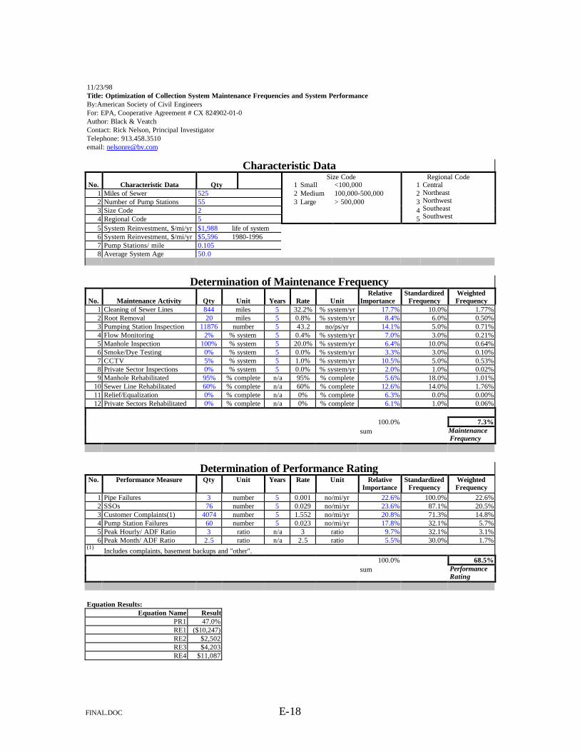
FINAL.DOC E-18

11/23/98Title: Optimization of Collection System Maintenance Frequencies and System PerformanceBy:American Society of Civil EngineersFor: EPA, Cooperative Agreement # CX 824902-01-0Author: Black & VeatchContact: Rick Nelson, Principal InvestigatorTelephone: 913.458.3510email: [email protected]

Characteristic DataSize Code Regional Code

No. Characteristic Data Qty 1 Small <100,000 11 Miles of Sewer 525 2 Medium 100,000-500,000 22 Number of Pump Stations 55 3 Large > 500,000 33 Size Code 2 44 Regional Code 5 5

CentralNortheastNorthwestSoutheastSouthwest

5 System Reinvestment, $/mi/yr $1,988 life of system6 System Reinvestment, $/mi/yr $5,596 1980-19967 Pump Stations/ mile 0.1058 Average System Age 50.0

Determination of Maintenance Frequency

No. Maintenance Activity Qty Unit Years Rate UnitRelative

ImportanceStandardized

FrequencyWeightedFrequency

1 Cleaning of Sewer Lines 844 miles 5 32.2% % system/yr 17.7% 10.0% 1.77%2 Root Removal 20 miles 5 0.8% % system/yr 8.4% 6.0% 0.50%3 Pumping Station Inspection 11876 number 5 43.2 no/ps/yr 14.1% 5.0% 0.71%4 Flow Monitoring 2% % system 5 0.4% % system/yr 7.0% 3.0% 0.21%5 Manhole Inspection 100% % system 5 20.0% % system/yr 6.4% 10.0% 0.64%6 Smoke/Dye Testing 0% % system 5 0.0% % system/yr 3.3% 3.0% 0.10%7 CCTV 5% % system 5 1.0% % system/yr 10.5% 5.0% 0.53%8 Private Sector Inspections 0% % system 5 0.0% % system/yr 2.0% 1.0% 0.02%9 Manhole Rehabilitated 95% % complete n/a 95% % complete 5.6% 18.0% 1.01%

10 Sewer Line Rehabilitated 60% % complete n/a 60% % complete 12.6% 14.0% 1.76%11 Relief/Equalization 0% % complete n/a 0% % complete 6.3% 0.0% 0.00%12 Private Sectors Rehabilitated 0% % complete n/a 0% % complete 6.1% 1.0% 0.06%

100.0% 7.3%sum Maintenance

Frequency

Determination of Performance RatingNo. Performance Measure Qty Unit Years Rate Unit Relative

ImportanceStandardized

FrequencyWeightedFrequency

1 Pipe Failures 3 number 5 0.001 no/mi/yr 22.6% 100.0% 22.6%2 SSOs 76 number 5 0.029 no/mi/yr 23.6% 87.1% 20.5%3 Customer Complaints(1) 4074 number 5 1.552 no/mi/yr 20.8% 71.3% 14.8%4 Pump Station Failures 60 number 5 0.023 no/mi/yr 17.8% 32.1% 5.7%5 Peak Hourly/ ADF Ratio 3 ratio n/a 3 ratio 9.7% 32.1% 3.1%6 Peak Month/ ADF Ratio 2.5 ratio n/a 2.5 ratio 5.5% 30.0% 1.7%

(1) Includes complaints, basement backups and "other".

100.0% 68.5%sum Performance

Rating

Equation Results:Equation Name Result

PR1 47.0%RE1 ($10,247)RE2 $2,502RE3 $4,203RE4 $11,087

Documents

Optimization of Collection System Maintenance Frequencies ... · Optimization of Collection System Maintenance Frequencies and System Performance Prepared by Black & Veatch LLP for