UNLV Retrospective Theses & Dissertations

1-1-2008

Optimization of bipolar plate design for flow and temperature Optimization of bipolar plate design for flow and temperature

distributions using numerical techniques distributions using numerical techniques

Kiran Mohan Veepuri University of Nevada, Las Vegas

Follow this and additional works at: https://digitalscholarship.unlv.edu/rtds

Repository Citation Repository Citation Veepuri, Kiran Mohan, "Optimization of bipolar plate design for flow and temperature distributions using numerical techniques" (2008). UNLV Retrospective Theses & Dissertations. 2366. http://dx.doi.org/10.25669/fka1-dqh3

This Thesis is protected by copyright and/or related rights. It has been brought to you by Digital Scholarship@UNLV with permission from the rights-holder(s). You are free to use this Thesis in any way that is permitted by the copyright and related rights legislation that applies to your use. For other uses you need to obtain permission from the rights-holder(s) directly, unless additional rights are indicated by a Creative Commons license in the record and/or on the work itself. This Thesis has been accepted for inclusion in UNLV Retrospective Theses & Dissertations by an authorized administrator of Digital Scholarship@UNLV. For more information, please contact digitalscholarship@unlv.edu.

OPTIMIZATION OF BIPOLAR PLATE DESIGN FOR FLOW AND TEMPERATURE

DISTRIBUTIONS USING NUMERICAL TECHNIQUES

by

Kiran Mohan Veepuri Bachelor o f Engineering in Mechanical Engineering

Osmania University, India 2005

A thesis submitted in partial fulfillment o f the requirements for the

Master o f Science Degree in Mechanical Engineering Department o f M echanical Engineering

Howard R. Hughes College of Engineering

Graduate College University of Nevada, Las Vegas

August 2008

UMI Number: 1460486

INFORMATION TO USERS

The quality of this reproduction is dependent upon the quality of the copy submitted. Broken or indistinct print, colored or poor quality illustrations and photographs, print bleed-through, substandard margins, and improper alignment can adversely affect reproduction.

In the unlikely event that the author did not send a complete manuscript and there are missing pages, these will be noted. Also, if unauthorized copyright material had to be removed, a note will indicate the deletion.

UMIUMI Microform 1460486

Copyright 2009 by ProQuest LLC.

All rights reserved. This microform edition is protected against

unauthorized copying under Title 17, United States Code.

ProQuest LLC 789 E. Eisenhower Parkway

PC Box 1346 Ann Arbor, Ml 48106-1346

IJNTV Thesis ApprovalThe G raduate College U niversity of N evada, Las Vegas

0 9 t h JULY . 2onm

The Thesis prepared by

KIRAN MOHAN VEEPURI

Entitled

OPTIMIZATION of BIPOLAR PLATE DESIGN for FLOW and TEMPERATURE DISTRIBUTIONS USING NUMERICAL TECHNIQUES

is approved in partial fulfillment of the requirem ents for the degree of

MASTER OF SCIENCE IN MECHANICAL ENGINEERING

(TExam ination C om m ittee M em ber

2 ^Exam ination Com m ittee M em ber

G raduate College FjjetlJty R epresentative

Examinamon Com m ittee Chair

Dean o f the Graduate College

11

ABSTRACT

Optimization of Bipolar Plate Design for Flow and Temperature Distributions UsingNumerical Techniques

by

Kiran Mohan Veepuri

Dr. Yitung Chen, Examination Committee Chair Associate Professor o f Department o f Mechanical Engineering

University o f Nevada, Las Vegas

Although water is fed eontrollably into the flow channels in the bipolar plates

surrounding the membrane electrode assembly (MEA), the complex flow geometry can

lead to non-uniformity o f the flow and temperature distribution inside the channels. In

addition, non-uniform temperature distribution in the cell will affect the electrochemical

process for hydrogen production or fuel cell applications. There are many studies on the

theoretical analysis o f fuel cells, but not many have been reported on the characteristics

o f the PEM electrolyzer.

In this thesis work, numerical simulations were carried out on the basic bipolar

plate given by the Proton Energy Systems in the United States. A 3-D steady state,

incompressible flow model was developed. Finite volume method was used to solve the

model for flow and temperature distributions inside the ehannels o f the bipolar plate.

Ill

A parametric study was performed based on number o f inlets and outlets and an

optimized bipolar plate design was selected. Later, the optimized model was again

simulated for two-phase flow. The flow and temperature distributions inside the channels

o f the new bipolar plate design were found to be uniform even for two-phase flow. Again

a parametric study was performed based on volumetric flow rate o f water and mass flow

rate o f oxygen production. Results were tabulated and numerical values were compared

with the back o f the envelope calculations.

IV

TABLE OF CONTENTS

ABSTRACT....................................................................................................................................... üi

LIST OF FIGURES .........................................................................................................................vii

N OM EN CLATURE............................................ viii

ACKNOWLEDGEMENTS............................................................................................................. x

CHAPTER 1 INTRODUCTION ................................................................................................... 11.1 Global p ic tu re ........................................................................................................................ 11.2 H ydrogen................................................................................................................................51.3 E lectro lyzer........................................................................................................................... 5

1.3.1 Alkaline electro lyzer.................................................................................................. 71.3.2 Solid oxide electrolyzer ............................................................................................ 71.3.3 Proton exchange membrane electro lyzer...............................................................8

1.3.3-1 M em brane.....................................................................................................101.3.3-2 Electrocatalyst .............................................................................................101.3.3-3 Bipolar plate ................................................................................................ 12

1.4 Literature re v ie w ................................................................................................................ 131.5 Objective o f research ........................................................................................................ 16

CHAPTER 2 PROBLEM DESCRIPTION AND NUMERICAL M ODELING................172.1 Problem description .......................................................................................................... 172.2 Governing equations .........................................................................................................202.3 Numerical m e th o d ............................................................................................................. 21

2.3.1 Finite volume method ............................................................................................. 212.3.2 Segregated solution algorithm ...............................................................................22

2.4 Boundary conditions .........................................................................................................232.4.1 Velocity inlet boundary condition ...................................................................... 232.4.2 Pressure outlet boundary cond ition ..................................................................... 242.4.3 Thermal boundary cond ition .................................................................................242.4.4 Wall boundary condition ........................................................................................25

CHAPTER 3 NUMERICAL MODELING FOR THE FLOW AND TEMPERATURE DISTRIBUTION IN THE BIPOLAR PLATE .......................................................................... 26

3.1 Baseline design analysis .................................................................................................. 263.2 Mesh independent study .................................................................................................. 273.3 Velocity distribution .........................................................................................................30

V

CHAPTER 4 DESIGN OPTIMIZATION OF THE BIPOLAR PLATE FOR UNIFORM FLOW AND TEMPERATURE DISTRIBUTION ..................................................................33

4.1 Reason for non-uniform f lo w .......................................................................................... 334.2 Design Modification .........................................................................................................35

4.2.1 Case-1 ........................................................................................................................354.2.2 Case-2 ........................................................................................................................384.2.3 Case-3 ........................................................................................................................404.2.4 Case-4 ........................................................................................................................43

4.3 Conclusion .......................................................................................................................... 45

CHAPTER 5 HYDRODYNAMIC ANALYSIS ON TW O-PHASE F L O W ......... 465.1 Need for two-phase f lo w ..................................................................................................465.2 Introduction to two-phase f lo w .......................................................................................475.3 Model set-up .......................................................................................................................495.4 Results and parametric study .......................................................................................... 50

5.4.1 Case-1 ........................................................................................................................505.4.2 Case-2 ........................................................................................................................515.4.3 Case-3 ........................................................................................................................ 52

5.5 V alidation .............................................................................................................................53

CHAPTER 6 CONCLUSIONS AND FUTURE WORK RECOMMENDATIONS ....... 586.1 C onclusions......................................................................................................................... 586.2 Future recom m endations.................................................................................................. 59

REFERENCES ................................................................................................................................. 61

V IT A ................................................................................................................................................... 66

VI

LIST OF FIGURES

Figure 1.1 Global fossil carbon emissions in last two cen tu ries .........................................2Figure 1.2 Renewable energies used in year 2005 .................................................................4Figure 1.3 Monopolar d e s ig n ......................................................................................................6

Figure 1.4 Bipolar d es ig n .............................................................................................................6

Figure 1.5 Schematic diagram of a PEM electro lyzer.......................................................... 9Figure 2.1 PEM electrolysis c e l l .............................................................................................. 17Figure 2.2 Flow distribution o f water in channels o f the bipolar p la te ........................... 18Figure 2.3 Computer aided design (CAD) model o f bipolar plate .................................. 19Figure 2.4 Iterative solution method for the segregate solver .......................................... 23Figure 3.1(a) Computational mesh model o f the bipolar plate .............................................. 28Figure 3.1(b), (c) & (d) Closer image o f the grid inside the channels with element density

4, 6 and 8 , respectively .......................................................................................... 29Figure 3.2 Mesh independent study p lo t ................................................................................ 30Figure 3.3 Velocity distributions inside the channels o f the bipolar plate & CAD model

showing plane o f cut AA & B B ........................................................................... 31Figure 4.1 CAD model o f the baseline design (Isometric view) ......................................34Figure 4.2 New bipolar plate design: Case-1 ........................................................................35Figure 4.3 Velocity distribution plot and pressure contour; Case-1 ..... 37Figure 4.4 Temperature contour; Case-1 ............................................................................... 37Figure 4.5 CAD model o f the bipolar plate with one inlet and outlet; Case-2 ..............39Figure 4.6 Velocity distribution plot and pressure contour; Case-2 ................................39Figure 4.7 Temperature contour; Case-2 ............................................................................... 40Figure 4.8 CAD model o f the bipolar plate with two inlets and outlets; Case-3 ............41Figure 4.9 Velocity distribution plot and pressure contour; Case-3 ................................42Figure 4.10 Temperature contour; Case-3 ............................................................................... 42Figure 4.11 CAD model o f the bipolar plate with four inlets and outlets; Case-4 ...........43Figure 4.12 Velocity distribution plot and pressure contour: Case-4 ................................ 44Figure 4.13 Temperature contour; Case-4 ............................................................................... 44Figure 5.1 H alf section o f the new bipolar plate CAD model with four in le ts ...............49Figure 5.2 Velocity profile for two-phase flow ....................................................................51Figure 5.3 Velocity profile for 0.3 1pm water and 0.01 g/s o x y g en ...................................52Figure 5.4 Velocity profile for 1.5 1pm water and 0.06 g/s o x y g en ...................................53Figure 5.5 VOF o f oxygen at outlet in case-1 ........................................................................ 55Figure 5.6 VOF o f oxygen at outlet in c a se -2 ........................................................................ 55Figure 5.7 VOF o f oxygen at outlet in case-3 ........................................................................ 56

Vll

NOMENCLATURE

Cp Specific heat at constant pressure, J-kg''-K ''

D Hydraulic diameter, m

F Body force, N

g Acceleration due to gravity, m-s’

K Coefficient o f thermal conductivity, W -m ''K‘'

n Number o f phases

AP Pressure drop. Pa

p Static pressure. Pa

Q Volumetric flow rate, m^-s"'

Re Reynolds number

Sh Heat o f chemical reaction, kg-K m'^-s'"

T Temperature, K

Ui Mean veloeity eomponent (i = 1, 2, 3), m-s''

Uj Mean velocity component (j = 1, 2, 3), m-s''

Uk Mean velocity component (k = 1, 2, 3), m-s''

^ Velocity o f the fluid

^ Mass-averaged velocity, m-s '

Drift velocity for secondary phase k

vm

Wi Length coordinate i (x,y,z), m

Wj Length coordinate j (x,y,z), m

w* Length coordinate k (x,y,z), m

X Thermal conductivity, W-m"'K"'

p Dynamic viscosity, kg-m'" s"'

Viscosity o f mixture, kg-m ''-s''

V Kinematic viscosity, m^-s'’

p Density, kg m'^

Mixture density, kg m'^

Density o f phase k, kg-m''^

Volume fraction

IX

ACKNOWLEDGMENTS

This thesis is the end o f my journey in obtaining my Masters o f seience degree in

mechanical engineering. I have not traveled in a vacuum in this journey. There are some

people who made this journey easier with words o f encouragement and more

intellectually satisfying by offering different places to look to expand my theories and

ideas.

First a very special thank you to Dr. Yitung Chen.

Dr. Yitung Chen gave me the confidence and support to begin my M aster’s

program in Computational Fluid Dynamics. Dr. Chen challenged me to set my

benchmark even higher and to look for solutions to problems rather than focus on the

problem. 1 learned to believe in my work and myself. Thank you Professor.

1 would also like to gratefully acknowledge the support o f some very special

individuals. Dr. Jianhu Nie, who took me on the process o f learning and made him self

available even through his heavy work and teaching schedule. Thank you doesn’t seem

sufficient but it is said with appreciation and respect.

1 would like to thank Dr. Robert F Boehm and Dr. Rama Yenkat for their time in

reviewing the prospectus, participation o f defense as the committee members.

1 would like to thank the U.S. Department o f Energy and University o f Nevada

Las Vegas for their continuous support throughout the entire research.

Ashwin Nambakam, Anushaw Nambakam, Avinash Ramani and Radhika

Varadarajan; without their support, pursuing graduate study would not have been

possible. Their beliefs that one should face the challenges boldly instead o f leaving the

battlefield allowed me the freedom to pursue my Masters. Thank you all.

And to my brother Madan Mohan Veepuri who from day one saw me graduating

and in a way is a proxy for my father ever since my father passed away.

Finally, 1 would like to thank my mother Jay a Veepuri. Words cannot describe her

enormous support and encouragement in pursuing my Masters.

XI

CHAPTER 1

INTRODUCTION

1.1 Global Picture

One o f the main reasons for many people doing research on Proton Exchange

Membrane Electrolysis Cell (PEMEC) for production o f hydrogen is “Global warming”.

Global warming is the increase in the average temperature o f the Earth’s near-surface air

and oceans. Increasing global temperature will cause sea level to rise, and is expected to

increase the intensity o f extreme weather events and to change the amount and pattern o f

precipitation. In the past century, Earth’s temperature has risen about 1°F. The global sea

levels have risen 4 to 8 inches [1]. The past 50 years o f warming has been attributed to

human activity. On Earth, the major greenhouse gases are carbon dioxide (CO2), methane

(CH4) and ozone.

Human activity since the industrial revolution has increased the concentration o f

various greenhouse gases, leading to increased radiative forcing from CO2 , CH4 ,

tropospheric ozone, chloro flouro carbons (CFCs) and nitrous oxide. In all, methane is a

more effective greenhouse gas than carbon dioxide, but its concentration is much smaller

so that its total radiative effect is only about a fourth o f that from carbon dioxide. Some

other naturally occurring gases contribute very small fractions o f the greenhouse effect.

The atmospheric concentrations o f CO2 and CH4 have increased by 31% and 149%

respectively since the beginning o f the industrial revolution in the mid-1700s [2]. Fossil

fuel burning has produced about three-quarters o f the increase in CO 2 from human

activity over the past 20 years. Fig. 1.1 shows the increase in the global fossil carbon

emissions in the last two centuries. The fossil carbon emissions in the beginning o f the

industrial revolution were in control. But, after 1850, it rose drastically and is expected to

increase at a higher rate in the future.

18OOO

Carbon EmissionsGlobal7000

- Total- Petroleum- Coal- Natural Gas- Cement Production

6000

5000

4000

;3000

2000

1000

1800 1850 1900 1950 2004

m>c

IV"oc

.u

O

Fig. 1.1 Global fossil carbon emissions in the last two centuries [3]

Another important reason for the increasing research work on production o f hydrogen

is, the above mentioned fuels are non-renewable energy sources. Non-renewable energy

is energy that comes from the ground and is not replaced in a relatively short amount o f

time. Fossil fuels are the main category o f non-renewable energy. Fossil fuels include;

coal, oil and natural gas. They currently provide more than 85% o f all the energy

consumed in the United States, nearly two-thirds o f the electricity and virtually all o f the

transportation fuels [4]. Moreover, the demand for fuels is expected to increase in the

next two decades. In an article written by Michael T. Klarke, in the weekly journal “The

Nation”, he stated that “we are nearing the end o f the petroleum age and have entered the

age o f insufficiency”. The Department o f Energy in the United States indicated that the

global output o f fuels would increase from 84 million barrels o f oil equivalent (mboe) per

day in 2005 to a projected 117.7 mboe in 2030 which is barely enough to satisfy the

anticipated world demand o f 117.6 mboe [5].

As a consequence, investigations o f renewable energy strategies have recently

become important, particularly for future world stability. The most important property o f

renewable energy sources is their environmental compatibility. In 2005 about 18% o f

global final energy consumption came from renewables [6 ]. Fig. 1.2. shows the different

kinds o f renewable sources used to generate energy in 2005. From this pie diagram it can

be found that more than 50% o f the renewable energy that is used is generated from

hydropower. Hydroelectricity is generated from hydropower and it does not produce

greenhouse gases. But, hydroelectric projects can be disruptive to the surrounding aquatic

ecosystems. The reservoirs o f hydroelectric power plants in tropical regions may produce

substantial amounts o f methane and carbon dioxide due to plant material in flooded areas

decaying in an anaerobic environment. Another important and serious reason is failure o f

large dams. The Banqiao Dam failure in southern China resulted in the deaths o f 171,000

people and left millions homeless [7]. Other ways o f producing energy from water is by

electrolysis. This is a very simple process. When current is passed through water, the

water is split into hydrogen (H2 ) and oxygen (O 2). The hydrogen thus produced can be

used as energy carrier in many applications.

2 H2 0 (1) ► 2 H2(g) + 0 2 (g) (Eq. 1.1)

Since chemical (H2 ) energy is being created, a minimum energy must be input to

drive the process according to the laws o f thermodynamics. In terms o f electrical energy,

this corresponds to a voltage greater than 1.23 V. In reality, the working voltage,

generally known as the over voltage, represents a waste o f energy or loss o f efficiency. It

has two main causes, one o f which is the internal voltage drop loss due to the finite

electrical resistance o f the electrolyte, or the membrane in this case. The second is kinetic

in origin, i.e., to do with the overall speed o f the process at the electrode surface. [8 ]

World Renewable Energy 2005

g Large hydro g Small hydro 5.12% n Wind power 4.58% Q Biomass elec58.23% 3.42%

g Geothermal eiec Photovoltaic 0.42% g C^hw elec** 0.05% g Biomass heat*0.72% 17.08%

g Solar he^ 6.83% H Geothermal heat [ ] BiocBesel fuel □ Bioethanol fuel2.17% 1.21% 0.16%

Fig. 1.2. Renewable energies used in year 2005 [6 ]

1.2 Hydrogen

While the fossil-fuel era enters its sunset years, a new energy regime is being born

that has the potential to remake civilization along radically new lines - hydrogen.

Hydrogen is the most basic and ubiquitous element in the universe. It can be used as fuel

in almost every application where fossil fuels are used. It never runs out and produces no

harmful CO2 emissions when burned; the only byproducts are heat and pure water.

Hydrogen power will reduce the CO 2 emissions and mitigate the effects o f global

warming. In the long run, the hydrogen-powered economy will fundamentally change the

very nature o f our market, political and social institutions, just as coal and steam power

did at the beginning o f the Industrial Revolution.

Hydrogen can be produced from a diverse array o f potential feedstocks, including

water fossil fuels and organic matter. Commercial bulk hydrogen is usually produced by

the steam reforming o f natural gas. But, this method o f hydrogen production is dependent

on a potentially limited and volatile natural gas supply. On the other hand, this process

results in moderate emissions o f CO2 and is not desirable. As discussed earlier, the better

way o f producing hydrogen is by electrolysis.

1.3 Electrolyzer

The electrolyzer is a device that generates hydrogen and oxygen from water

through the application o f electricity. It consists o f a series o f porous graphite plates

through which water flows while low voltage direct current is applied. An electrolyzer

stack consists o f several cells linked in series. These cells are o f two types namely mono-

polar and bipolar cell [9]. In the monopolar design the electrodes are either negative or

positive with parallel electrical connection o f the individual cells (Fig. 1.3), while in the

bipolar design the individual cells are linked in series electrically and geometrically

(Fig. 1.4). One advantage o f the bipolar cell design is that they are more compact than

monopolar systems which give shorter current paths in the electrical wires and electrodes.

This reduces the losses due to internal ohmic resistance o f the electrolyte, and therefore

increases the electrolyzer efficiency.

T"- f ” O r

1

Hz_

0

0

0

o'’ 0 0

J —— ....V

Hz O2 O,

cathode j anode diaphragm

/container

Fig. 1.3 M onopolar design [9]

Hz i O : '.H, Hz I O 2 H; Oz

-----T J-------0

i 0 0

0 o1 0

; 0 ^

1 ^

K} ° a

/y=î 0 a o .nrr." __

o - f

' \ X /cathode anode \(bipolar plate) diaphragm container

Fig. 1.4 Bipolar design [9]

1.3.1 Alkaline Electrolyzer

Alkaline electrolyzers usually use an alkaline solution o f sodium or potassium

hydroxide (NaOH or KOH) that acts as the electrolyte, mostly with 20-30 wt% because

o f the optimal conductivity, they require using corrosion resistant stainless steel to

withstand the chemical attack. These electrolyzers, generally, operate at a temperature o f

70-100°C and at a pressure o f 1-30 bar. The following are the two chemical reactions that

take place at anode and cathode finally resulting in the production o f hydrogen:

For the anode reaction it is:

4 H2 0 (1) + 4e -------- ► 2 H2 (g) + 40H'(aq) (Eq. 1.2)

For the cathode reaction it is:

40H'(aq) ► 02(g) + 4e' 4- 2Fl20(i) (Eq. 1.3)

And finally the overall electrolyzer reaction is:

2 H2Ü(|) ► 2 H2(g) + 0 2 (g) (Eq. 1.4)

1.3.2 Solid Oxide Electrolyzers

Solid oxide electrolyzers, which use a solid eeramic material as the electrolyte that

selectively transmits negatively charged oxygen ions at elevated temperatures, generate

hydrogen in a slightly different way -

• W ater at the cathode combines with electrons from the external circuit to form

hydrogen gas and negatively charged oxygen ions;

• The oxygen ions pass through the membrane and react at the anode to form

oxygen gas and give up the electrons to the external circuit.

Solid oxide electrolyzers must operate at temperatures high enough for the solid oxide

membranes to function properly (about 500 - 800°C; compared to PEM electrolyzers.

which operate at 80-100°C, and alkaline electrolyzers, which operate at 100-150°C). The

solid oxide electrolyzer can effectively use heat available at these elevated temperatures

to decrease the amount o f electrical energy needed to produce hydrogen from water. [ 1 0 ]

1.3.3 Proton Exchange Membrane Electrolyzer

Polymer electrolyte membranes (PEMs) were first developed for the chlor-alkali

industry. These specialized materials, also known as ionomers, are solid fluoro-polymers

which have been chemically altered to make them electrically conductive. The

fluorocarbon chain has typically a repeating structural unit, such as - [Cp2% CF2 ]n-, where

n is very large. Treatments like sulphonation or carboxylation, insert ionic or electrically-

charged pendant groups, statistically spaced, into some o f these base units giving, e.g.,

[CF(S0 3 .IT^) % CF2 ]m-, where m can range from n/5 to n/20 depending on the properties

most suited for the application. Nation, made by Du Pont, is the most commercially

successful o f such materials, and is available as thin pre-formed membranes in various

thicknesses, or as a 5% solution which may be deposited and evaporated to leave a

polymer layer o f customized shape. The electrolyzers that are based on polymer

electrolyte membrane separators are mostly used for industrial purposes because they can

achieve high efficiencies. These devices anticipate the imminent development o f a

renewable energy economy based on electricity and FI2 fuel as complementary energy

vector. [8 ]

A PEM electrolyzer is shown in Fig. 1.5. Its efficiency is a function primarily o f

the membrane, electrocatalysts and the bipolar plate. This becomes crucial under high-

current operation, which is necessary for industrial-seale application. The following

reactions occur in a PEM electrolyzer:

Reaction at anode;

2 H2 0 (I) —

Reaction at cathode:

4 H '^ ( a q ) + 4e"

► 4H ( a q ) + 4e" + 0 2 ( 2

-> 2H

2(g)

2(g)

Overall electrolyzer reaction:

2H20(|) ► 2H2(g) + 02(g)

(Eq. 1.5)

(Eq. 1.6)

(Eq. 1.7)

AAnode Calhod

PolyelectrolyteMembrane [PEM]

t" Protons'^ [H+]

electrocatalysts.

Electron flow

Fig. 1.5 Schematic diagram o f a PEM electrolyzer [9]

1.3.3-1 Membrane

The membrane consists o f solid fluoro-polymer which has been chemically

altered in part to eontain sulphonie acid groups, SO3H, which easily release their

hydrogen as positively-charged atoms or protons [8 ]:

SO3H 1 -:-:-» SO]- + H+ (Eq. 1.8)

These ionic or charged forms allow water to penetrate into the membrane structure but

not the product gases, molecular hydrogen (Hz) and oxygen (O2). The resulting hydrated

proton, H ]0^, is free to move whereas the sulphonate ion (SO3) remains fixed to the

polymer side-chain. Thus, when an electric field is applied across the membrane the

hydrated protons are attracted to the negatively charged electrode, known as the cathode.

Since a moving charge is identical with electric current, the membrane acts as a

conductor o f electricity. It is said to be a protonic conductor. A typical membrane

material that is used is called “Nation”. Because “N ation” is a solid, its acidity is self-

contained and so chemical corrosion o f the electrolyzer housing is much less problematic.

Furthermore as it is an excellent gas separator, allowing water to permeate almost to the

exclusion o f H] and O2 , it can be made very thin, typically only 100 microns. This

improves its conductivity so that the electrolyzer can operate effectively even at high

currents.

1.3.3-2 Electrocatalyst

A solid catalyst speeds up chemical reactions due to its surface action. As a

simple example, two H atoms held loosely on a surface are much more likely to collide

and make H2 gas than if they are dispersed in a liquid with billions o f water molecules in-

between. This is a spatial or localized concentration effect. The case o f O2 evolution is

10

much more complex. Two water molecules must be broken into their constituent atoms;

then the two O atoms must combine. The electrocatalyst at the anode is a special catalyst,

which facilitates this process by withdrawing electrons from the water such that the H

atoms are ejected as protons, which enter the membrane. Water is said to be activated by

charge-transfer. The OH or 0 atoms are very reactive in their free state. However, when

fixed at the surface by chemical bonds they are much more stable. W hen more water

encounters the surface, its protons are ejected in turn and O atom are accumulated. These

are then able to combine easily by surface diffusion just as described for hydrogen. It is

said that the surface provides a low-energy pathway, which is intrinsically much faster

because the speed o f the reaction is related exponentially to the energy difference.

It is easy to visualize that if the cathode and anode surfaces, respectively, attract H

or O atoms too strongly, the surfaces will become completely covered with these

intermediates and the catalytic process stops. On the other hand, if protons or water are

not attracted strongly enough, the process never gets going. Only when there is a

moderate strength o f binding o f reactants and intermediates at the electrode surfaces, the

right balance will be obtained. This is the key factor in determining if a solid catalyst will

work efficiently. It is also obvious that the larger the catalyst surface area available, the

more H i and O2 will be produced in a given time, i.e., a higher current will flow in the

electrolyzer.

Platinum is long known to be the best catalyst for water electrolysis due to its

moderate strength o f adsorption o f the intermediates o f relevance. It has the lowest over­

voltage o f all metals. However due to its cost, and the preferred operation o f the

electrolyzer at high current, ingenious ways have been devised to deposit ultra-fine Ft

11

particles either on the electrode support plate, or directly onto the membrane, which is

then clamped for good electrical continuity. A current o f 1-3 A/cm^ can be obtained from

as little as milligrams o f Pt spread over the same area. [11]

1.3.3-3 Bipolar Plate

The bipolar plates are in weight and volume the major part o f the PEM

electrolyzer cell stack, and are also a significant contributor to the stack costs. The

bipolar plate is therefore a key component if power density has to increase and costs must

come down. Bipolar plates have to accomplish many functions in the electrolyzer cell

stack. Main functions are:

• Distribution o f water uniformly over the active areas;

• Uniform thermal distribution to water from the membrane;

• Conduction o f current from cell to cell;

• Preventing leakage o f gases and coolant.

For uniform fluid flow distribution inside the channels o f the bipolar plate, tight

tolerances on channel dimensions have to be met. Small deviations lead to reduced

efficiency, poor utilization o f the catalyst and reduced hydrogen output and should

therefore be avoided. Uniform thermal distribution o f water in the channels is achieved

only if the flow distribution is achieved. To minimize the ohmic losses the material needs

to have low bulk resistance and low contact resistance [12]. Today several materials are

being used in bipolar plates.

12

1.4 Literature Review

Hydrogen production from water electrolysis using proton exchange membranes

has been studied to some degree since the development o f the first PEM water

electrolyzer by the General Electric Company [13]. Barbir [14] discussed the difference

between the electrical grid independent and grid assisted hydrogen generation. It is also

shown that electrolytically generated hydrogen from an integrated system o f both grid

connected and grid independent is stored and then via fuel cell converted back to

electricity when needed. Grigoriev et al. [15] discussed the effects o f the operating

temperature and pressure on the volt-amperic curves o f the electrolysis cell. The volt-

amperic curves o f electrolysis cell with different catalyst at 90°C were presented.

A theoretical model was proposed by Choi et al. [16], to explain the current-

potential characteristics o f PEM electrolysis cell based on the involved charge and mass

balances as well as Butler-Volmer kinetics on the electrode surfaces. It is found that the

reduction kinetics at the cathode is relatively fast while the anodic overpotential is mainly

responsible for the voltage drop.

A technology where the membrane itself is catalytically effective, splitting water

into protons and hydroxyl ions is described by Balster et al. [17]. A mature

electromembrane technology was reviewed. In addition, bipolar, ion-exchange membrane

technology was extensively described. The catalyst and absorbent technologies under

development for the extraction o f hydrogen from the natural gas to meet the requirements

from the PEMFC were discussed by Farrauto et al. [18]. Electrochemieal characterization

o f the various electrocatalytic powders was conducted in 0.5M H 2 SO4 electrolyte at room

temperature, by supporting the powders on titanium plates using a spraying technique

13

[19]. The performance o f the various anode electrocatalysts were evaluated in a single

PEM water electrolysis cell up to current densities o f 2 A cm'^ with the total (anode and

cathode) noble metal loadings less than 2 mg cm'^.

Millet et al. [20] discussed the design and performance o f a PEM water

electrolyzer. High cell voltages were contributed to poor electrical connections which

introduced a significant ohmic loss. Rasten [21] provided a study o f various

electrocatalysts for water electrolysis using proton exchange membrane. A solid polymer

electrolyzer was developed using IrOa as the anode catalyst and Pt black as the cathode

catalyst at loading o f 3 mg/cm^ [22].

Since 1987 Mitsubishi Heavy Industries, Ltd. has been developing solid polymer

water electrolyzer technology [23]. A chemical plating technique was used to plate

iridium metal onto each side o f the Nafion membrane. A 50 cm^ solid polymer electrolyte

electrolyzer was developed using a hot press method to adhere the catalyst film to the

membrane [24]. Based on the results mentioned above, a 2500 cm^ solid polymer

electrolyte electrolyzer was developed [25]. A high pressure solid polymer electrolyte

water electrolyzer was developed with Pt and Ir black serving as the anode catalyst and Pt

black as the cathode catalyst [26]. The development o f membrane electrode assemblies

(MEAs) for a reversible solid polymer fuel cell was examined using Pt, Rh, Ir, and Ir-Ru

mixed oxides, as the oxygen evolution electro-catalyst [27]. Millet [28] provided an

experimental study for an electrode membrane electrode (EME) cell operated at high

current densities. From their experimental work, the electric potential across the cell and

membrane alone were computed, since the determination o f anodic and cathodic over­

voltages usually requires the use o f a membrane strip [29, 30]. They also determined if a

14

membrane strip can be used as a reference potential to measure separately each term o f

the cell voltage.

A micro-scale model was developed by Zhou et al. [31] to predict the contact

resistance between the bipolar plate and the gas diffusion layer (GDL) in PEMFC.

Bipolar plate surface topology is simulated as randomly distributed asperities and gas

diffusion layer modeled as randomly distributed eylindrical fibers. Heinzel et al. [32]

discussed the method o f production o f low cost bipolar plates for PEM cells. M aterials

with low cost and high availability, high chemical resistance and good mechanical

properties were chosen for manufacturing o f bipolar plates. It was found that the cost for

production o f bipolar plate by injection moulding is very low. Injection moulding o f

composite bipolar plates for PEMFC compared with moulding technologies and the

production feasibility o f polypropylene based composites at different temperatures was

tested by Muller et al. [33]. Electrical and chemical stability o f the plates at different

temperatures was tested.

Barreras et al. [34] demonstrated that the flow distribution inside a bipolar plate

ean be visualized by applying laser-induced fluorescence in an optically accessible

model. A parallel-channel commercial bipolar plate with a transparent plastic plate cover

was investigated. A three-dimensional transient numerical model o f PEMFC was

developed and the effect o f gas flow-field design in the bipolar plates tested by Atul et al.

[35].

Most o f the research on the PEM electrolyzer cell so far, focused on the

experimental studies and numerical analysis o f the catalyst, electrolytic membrane and

membrane electrode assembly. Even though a little amount o f research work was done on

15

bipolar plate, no numerical analysis was done on the design optimization to obtain

uniform flow and temperature distribution. The main aim o f this thesis is to design a

bipolar plate which gives uniform flow and temperature distribution o f the fluid in the

channels.

1.5 Objective o f Research

The present work is funded by the Department o f Energy o f the United States

under award DE-FG36-03GO13063. Some o f the research objectives are outlined as

follows:

• To develop a computational model for the bipolar plate o f the PEM electrolyzer;

• To analyze the flow and temperature distribution o f the fluid inside the channels

o f the above developed bipolar plate;

• To redesign the bipolar plate so as to obtain homogeneous flow and temperature

distribution;

In the next chapter, the design o f the bipolar plate is described. The numerical

model and the operating and boundary conditions that will be used are also discussed.

Computational meshing and the mesh independent study will be discussed in Chapter 3.

After mesh independent study, the design optimization o f the bipolar plate in order to

achieve uniform flow and temperature distribution will be discussed in Chapter 4. The

new bipolar plate that is designed in Chapter 4 is again simulated for two-phase flow. The

results are shown in Chapter 5. In Chapter 6 , the numerical experiment performed for this

thesis is concluded and future work that can be done in order to achieve a good design in

other aspects also are pointed out.

16

CHAPTER 2

PROBLEM DESCRIPTION AND NUMERICAL MODELING

2.1 Problem Description

The PEM electrolysis cell is used to produce hydrogen from the water flowing

through the bipolar plate as discussed earlier in Chapter 1, when water comes in contact

with the catalyst surface. Fig. 2.1 shows the basic two-dimensional schematic picture o f

the PEM electrolysis cell. The well known catalyst that is used in this process is

platinum. This increases the cost o f hydrogen produced by this process. To improve the

cost efficiency o f this process, the platinum catalyst must be used in a much more

effective way.

PEM Electrolysis

Oxygen Pmwen Exehmng* Mennbran*SoSd Etoctrotyte

Fig. 2.1 PEM Electrolysis cell [36]

17

The effective use o f platinum is achieved by the uniform flow o f water in the

channels o f the bipolar plate. From the experiments done by Barreras et al. [34] and Atul

et al. [35], it can be found that the flow distribution o f water inside the channels o f the

bipolar plate is not uniform. Fig. 2.2 shows the distribution o f water inside the channels

o f the bipolar plate. The flow rate in the end side channels is more when compared with

the middle side channels. In this case the platinum catalyst is more effective in the ends

channels when compared with the middle channels. This results in low efficiency o f

hydrogen production.

To improve the efficiency o f the PEM electrolysis cell and to make maximum use

o f the platinum catalyst, a new bipolar plate has to be designed which gives uniform flow

o f water in the channels.

Fig. 2.2 Flow distribution o f water in channels o f the bipolar plate [34]

18

The geometry o f the bipolar plate o f the PEM electrolysis cell that is considered is

shown in Fig. 2.3.

0 . 08” 0

Fig. 2.3 Computer aided design (CAD) model o f bipolar plate

The above shown bipolar plate consists o f 60 channels, each with a width o f 0.08

inches and a height o f 0.035 inches. The length o f each channel is 9.52 inches. The

channels are connected to one inlet and one outlet with the header section, which is one

inch in width and 9.52 inches in length. The inlet and outlet are circular in cross-section

with 1 inch diameter. The header is designed with cylindrical pellets in it. This changes

the flow direction o f water and helps to flow into the channels.

19

The water is fed into the bipolar plate from the inlet with a volumetric flow rate o f

0.3 liters per minute (1pm). The velocity o f the water is assumed to be uniform at the

entrance o f the inlet along the cross-sectional area. The properties o f water like density

and viscosity etc. are considered at a temperature o f 80°C. The bottom surfaces o f all the

channels will be in contact with the catalyst layer. This surface is known as active region

as shown in Fig. 2.3. A eonstant heat flux o f 2500 W/m^ is applied to the surfaces at the

bottom of the bipolar plate.

To know whether the flow inside the bipolar plate is laminar or turbulent, the

Reynolds number is calculated. The Eq. 2.1 below shows the formula to calculate the

Reynolds number (Re):

Re = ^ (Eq. 2.1)A

Here “ p ” and “ / /” are the density and viscosity o f the water. “ i9” is the velocity o f the

water at the inlet and “D ” is the hydraulic diameter o f the inlet. In this case the hydraulic

diameter is simply the diameter o f the inlet area. The value o f the Reynolds number for

the above boundary conditions is 172. This value is much less than 2400. Therefore this

model falls in the laminar flow region. Thus, laminar, incompressible flow model was

used for further calculations.

2.2 Governing Equations

The steady state governing equations for continuity, momentum and energy for

laminar flow can be expressed as follows:

= 0 0 & F 2 2 )

20

:r--(/3w,Wt) = (luq. :2.3)C W . 6Wy C W i CAVi^

™ ( w r ) = ^ U ^ ) + S„ (Eq.2.4)m r 6W, Cj> a v.

2.3 Numerical Method

The flow o f water through the micro channels o f the bipolar plate and the

complex geometry o f the bipolar plate make the study o f the flow distribution difficult.

To simplify the analysis, the physical model is replaced by infinite points and 3-D

elements. The points are known as grid-points or nodes. The 3-D elements are o f three

types: hexahedrals, tetrahedrons and prisms. These elements are known as grid elements

or cells. These nodes and cells define the entire geometry and this model is known as

finite element (FE), finite volume (FV) or finite difference (FD) model depending on the

type o f numerical method used. For the current numerical experiment, finite volume

method (FVM) is followed. When the above mentioned mathematical governing

equations will be solved for this model, it gives very close results o f pressure,

temperature, velocity distributions etc when compared the actual physical device. The

governing equations will be solved only at the grid points representing the geometry.

The computational mesh model o f the geometry is obtained from the commercial

software FlYFERMESFI 7.0 and is solved in the Cartesian coordinate system using the

general purpose CFD code FLUENT 6.3.26 which is based on finite volume method.

FLUENT is powerful commercial software for solving fluid flow, heat transfer and

chemical reaction problems [37].

21

2.3.1 Finite Volume Method

The finite volume method (FVM) is one o f the most versatile discretization

techniques used in computational fluid dynamics (CFD). Based on the control volume

formulation o f analytical fluid dynamics, the first step in the FVM is to divide the domain

into a number o f control volumes (elements) where the variable o f interest is located at

the centroid o f the control volume. The next step is to integrate the differential form o f

the governing equations over each control volume. Interpolation profiles are then

assumed in order to describe the variation o f the concerned variable between the cell

centroids. The resulting equation is called the discretized or discretization equation. In

this manner, the discretization equation expresses the conservation principle for the

variable inside the control volume.

The most compelling feature o f the FVM is that the resulting solution satisfies the

conservation o f quantities such as mass, momentum, energy and species. This is exactly

satisfied for any control volume as well as for the whole computational domain and for

any number o f control volumes. Even a proper coarse grid solution may exhibit similar

integral balances. It is also prefemed while solving partial differential equations

containing discontinuous coefficients.

2.3.2 Segregated Solution Algorithm

fhe segregated solver was used to solve the governing integral equations for the

conservation o f mass, momentum and energy equations. The numerical scheme that is

used in this study is first order upwind scheme and SIMPLE (semi-implicit method for

pressure-linked equations) algorithm is used to resolve the coupling between pressure and

velocity. The discrete and nonlinear governing equations are linearized using an implicit

7 0

formulation with respect to a set o f dependent variables in every computation cell. The

resulting algebraic equations are solved iteratively using an additive correction multi-grid

method with Gauss-Seidel relaxation procedure.

n oC onverged?

U pdate p ropeities.

Solve m om entum equations.

Solve energy, species, and o ther equations.

Solve pressure-correction (continuity) equation. U pdate pressure, face m ass flow rate.

Fig. 2.4 Iterative solution method for the segregate solver

2.4 Boundary Conditions

2.4.1 Velocity Inlet Boundary Condition

The velocity inlet boundary condition is used to define the flow velocity, along

with all other relevant sealar properties o f the flow, at the flow inlets. User can define the

inflow velocity by specifying the velocity magnitude and direction, the velocity

component, or the velocity magnitude normal to the boundary. I f the cell zone adjacent to

23

the veloeity inlet is moving, the user ean specify either relative or absolute velocities. In

this case, the velocity magnitude and direction type was used.

2.4.2 Pressure Outlet Boundary Condition

Pressure outlet boundary conditions require the specification o f a static (gauge)

pressure at the outlet boundary. The value o f the specified static pressure is used only

while the flow is subsonic. If the flow beeomes locally supersonic, the specified pressure

will no longer be used; pressure will be extrapolated from the flow in the interior. All

other flow quantities are extrapolated from the interior. A set o f “backflow” conditions is

also specified should the flow reverse direction at the pressure outlet boundary during the

solution process. Convergence difficulties will be minimized if the user specifies realistic

values for the backflow quantities.

2.4.3 Thermal Boundary Condition

This type o f boundary condition is defined only when the energy equation is

chosen to solve. At flow inlets and outlets, the temperatures are set. At the walls the

following thermal conditions can be used:

• Specified heat flux

• Specified temperature

• Convective heat transfer

• External radiation

• Combined external radiation and external eonvective heat transfer

In the current study case, speeified heat flux is speeified at the walls that come in

contact with the platinum catalyst and the inlet temperature is also set.

24

2.4.4 Wall Boundary Conditions

This type o f boundary conditions are used to bound the fluid and solid regions. In

viscous flows (which is considered in the current numerical experiment), the no-slip

boundary condition is enforced at the walls. Several other pieces o f information that can

be given under the wall boundary condition are shear conditions, wall roughness etc. But,

for this numerical experiment all these conditions are neglected.

25

CHAPTER 3

NUMERICAL MODELING FOR THE FLOW AND TEMPERATURE

DISTRIBUTION IN THE BIPOLAR PLATE

3.1 Baseline Design Analysis

The purpose o f the numerical analysis o f the bipolar plate o f PEMEC is to check

the flow distribution o f the water inside the channels and also the temperature distribution

in the fluid due to the constant heat flux supplied to channels from the bottom o f the

channels. The analysis is done on the baseline design o f the bipolar plate and then

studied. If the flow and temperature distribution inside the channels is not uniform then it

has to be redesigned so as to achieve uniform distribution o f flow and temperature. For

analysis, as mentioned in the earlier chapters, meshing is done using the powerful

commercial software HYPERMESH 7.0 and then simulation is done using the FLUENT

software. Different zones like inlet, outlet, walls etc. are set up in HYPERMESH and

then the boundary conditions are incorporated using FLUENT. The different boundary

conditions specified for the current model are:

• Inlet volumetric flow rate : 0.3 1pm

• Inlet temperature : 80°C

• Operating pressure : 1 atm

Heat flux : 2500 W/m 2

26

All the walls that bound the fluid, other than the walls that come in contact with the

catalyst, are assumed to be adiabatic. The properties o f water like density, viscosity, etc.

are taken at 80°C. From the calculations o f Reynolds number (Re=172) it is known that

water flow falls into laminar flow range; so laminar, incompressible flow model is set up

for the analysis. Once the model is set up, it is simulated for several iterations until the

solution is converged according to the absolute iterative convergence criterion. The

absolute convergence criterion is used by setting the absolute criteria to 10'^. After the

simulation, the results are plotted and the conclusions are made. But in this whole

process, the results obtained need to be mesh independent. This is done by performing a

mesh independent study.

3.2 Mesh Independent Study

A mesh independent study otherwise known as grid independent study plays a

very important study in the finite element analysis (FEA), finite difference method

(FDM) and finite volume method (FVM). After the given CAD model is divided into

finite elements and simulated, the obtained results are plotted. W hen the same model is

refined and simulated it gives different results. This variation is because o f the fact that

the results obtained after simulation depends on the grid. In order to avoid this, a grid

independent study is performed through which the percentage o f error can be minimized.

Once the percentage error is with in the tolerance limit, it can be said that the model with

that mesh is grid independent.

In the current numerieal experiment, the grid independent study is done for fluid

flow analysis alone. Since the aim o f this experiment is to achieve uniform flow

27

distribution inside the channels, the grid independent study is also done by varying the

number o f elements across the width o f the channels. Fig. 3.1 (a) shows the

computational mesh model and Fig 3.1 (b), (c) and (d) show different number o f mesh

elements inside the channels.

Fig 3.1(a) Computational mesh model o f the bipolar plate

28

:

m p

& i i m

Fig 3.1(b) Fig 3.1(c)

H g 3 JU 0 )

Fig 3.1 (b), (c) & (d) Closer images o f the grid inside the channels with element density

4, 6 and 8 , respectively

29

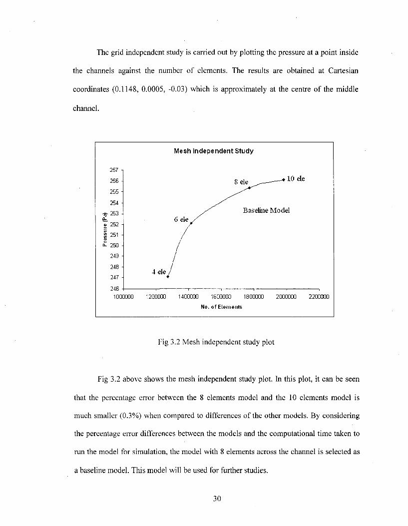
The grid independent study is carried out by plotting the pressure at a point inside

the channels against the number o f elements. The results are obtained at Cartesian

coordinates (0.1148, 0.0005, -0.03) which is approximately at the centre o f the middle

channel.

Mesh Independent Study

257 -,

1 0 ele256 - 8 ele255 -

254 -Baseline Model253 -

6 ele® 252 -

s 251

CL 250 -

249 -

248 -4 ele /

247 -

246 1-----1000000 1200000 140000G 1600000 22000001800000 2000000

No. of Elenieiits

Fig 3.2 M esh independent study plot

Fig 3.2 above shows the mesh independent study plot. In this plot, it can be seen

that the percentage error between the 8 elements model and the 1 0 elements model is

much smaller (0.3%) when compared to differences o f the other models. By considering

the percentage error differences between the models and the computational time taken to

run the model for simulation, the model with 8 elements across the channel is selected as

a baseline model. This model will be used for further studies.

30

3.3 Velocity Distribution

As mentioned earlier, the mesh independent study was carried out for fluid flow

analysis. After the mesh independent study was done and the baseline model was

selected, the fluid flow distribution inside the channels was studied. The velocity

distribution inside the channels is plotted for the baseline model and is shown in Fig 3.3.

0.04

0.03

Î>

0.02

0.01

0 0.05 0.1 0.15X ( m )

0.2

Fig 3.3 Velocity distribution inside the channels o f the bipolar plate & CAD model

showing plane o f cut AA & BB

31

The CAD figure shown in Fig 3.3, along with the velocity plot shows the plane o f

cut where the slice is taken to plot the results with help o f the AA and BB. The plane BB

is along the channel at a half the height o f the channels. From this figure it is clear that

the flow distribution inside the channels is not uniform. In the end channels, where the

velocity is very high, the water molecules might not stay in contact with the catalyst layer

for sufficient amount o f time for the reaction to take place. And in the middle channels,

where the movement o f water molecules is very slow, if the time taken by the water

molecules to move on the catalytic surface is more than the reaction time it leads to the

shortage o f water for the reaction to take place at the surface. This leads to the improper

use o f the catalyst. And since the catalyst that is generally used in a PEM electrolysis cell

is platinum, which is very costly, the production cost goes up. This indirectly means the

efficiency o f the PEM electrolysis cell is less which is undesirable.

To reduce the production cost o f the hydrogen using a PEM electrolysis cell, a

new bipolar plate has to be designed which gives a uniform flow distribution inside all

the channels.

In Chapter 4, several configurations o f bipolar plates that are designed and

simulated to achieve uniform flow will be discussed. These designs will also be studied

for the thermal distribution inside the channels. For a good bipolar plate the uniform

distribution o f temperature is also very important. Finally, optimized design o f the bipolar

plate will be chosen from those designs. This design will be used as the new bipolar plate

for further analysis.

32

CHAPTER 4

DESIGN OPTIMIZATION OF THE BIPOLAR PLATE FOR UNIFORM FLOW AND

TEMPERATURE DISTRIBUTION

4.1 Reason for Non-Uniform Flow

In the previous chapter, it is shown that the baseline design o f the bipolar plate

gives the non-uniform flow distribution inside the channels. In this chapter, the design

will be changed and simulated to achieve uniformity. But, to change the design, one

should first know the reason for the non-unifoimity. If that is known, then i f 11 be easy to

rectify it by changing the design in the areas where it is required.

The isometric view o f the baseline design along with the coordinate axes is shown

in Fig 4.1. This figure helps in understanding the flow o f water inside the bipolar plate

along with the direction. The water is fed into the bipolar plate from the inlet duct in

negative y-direction flows into the header along the 7 intermediate channels that connect

inlet duct and the header. Because o f this, the flow direction is changed to negative x-

direction. Here, one should make a note that the velocity vector is not exactly in the

negative x-direction. There will be non-zero y and z components o f the velocity o f the

water. Due to the z-component velocity vector, as soon as the water enters the header,

some amount o f the water is diverted in z direction and enters the initial channels. In the

later section o f the header, the water is deflected because o f the cylindrical pellets inside

the header. Even though the water is deflected, the major component o f the velocity

vector will be in the x-direction. So, the water moves completely to the end o f the header

in the negative x-direction and when it is blocked by the wall, it changes its direction and

enters the end channels with high velocity. Due to the deflection because o f the pellets

some amount o f water enters the middle channels, but the amount o f water that enters the

end channels is more when compared with the amount that enters the middle channels.

HEADER

AINLET 4^

Fig 4.1 CAD model o f the baseline design (Isometric view)

34

In order to achieve the uniform flow, changes should be made in the header in

such a way that same amount o f water is fed into the middle channels as in the end

channels. In the next few sections, several modifications made in the design will be

discussed as different cases.

4.2 Design Modification

4.2.1 Case-1

Since the flow direction in the channels is positive z-direction, it is better if the

water in the header also flows in the z-direction. Taking this point into consideration, a

new bipolar plate is designed which is shown in Fig 4.2.

0.793"

CDChro

Fig 4.2 New bipolar plate design; Case-1

35

The new bipolar plate designed has 6 inlets and 6 outlets as shown in Fig 4.2. The

number six for inlets and outlets was selected randomly. As the total number o f channels

is sixty, it was assumed that one inlet duct should supply water sufficiently to 1 0

channels. The centers o f the inlet and outlet ducts are at a distance o f 1.5 inches from the

entrance and exit o f the channels respectively. Even though the number o f inlets and

outlet is changed, the diameter o f the ducts still remains the same (1 inch). All the inlet

and outlet ducts are placed at equal distances, such that each duct covers 1 0 channels.

The Mesh was generated for this geometry with 8 elements across the channels and then

simulated to study the flow and temperature distribution inside the channels.

In this case, the energy equation is solved to know the temperature distribution

inside the channels when a constant heat flux is supplied. The model is run for the same

operating conditions and in the boundary conditions, a constant heat flux o f 2500 w W is

supplied to the channels from the bottom surface. Even though the volumetric flow rate is

not changed (0.3 1pm), the inlet velocity which is defined in FLUENT is reduced since

the number o f inlet ducts increased. Thus the Reynolds number is dropped to 114. After

the model is run for the mentioned boundary and operating conditions, a velocity

distribution plot and a temperature distribution contour were plotted. The slice was taken

at the same place as mentioned earlier in Chapter 3. Fig 4.3 shows the velocity

distribution and pressure distribution and Fig. 4.4 shows temperature distribution inside

the bipolar plate.

36

1.4

1.2

1 * 0 8

E% 0.6

0.4

0.2

P r e s s u r e (P a )5.0•SO4-Û3020100

- 1 0-20-SO^ - 0

0 Hiiiiiiimimiiiuiiniiiiiiiiimiiimiiiuniuiiiiiii0 0.05 0.1 0.15 0.2

X(m)

Fig 4.3 Velocity distribution plot and pressure contour: Case-1

356.8356.6

356.2

355.8355.6355.4355.2

354.4354.2

Tem perature (k)

Fig 4.4 Temperature contour: Case-1

37

The velocity profile drawn in Fig 4.3 shows that the velocity in each channel. The

mean velocity o f was found to be 0.083 m/s and the percentage deviation o f velocities in

each channel was found to be 3.87%. With this it can be said that there is uniform flow

distribution inside the channels and the pressure distribution reads the pressure drop

between the inlet and outlet around 100 Pa. From Fig 4.4 it is clear that even the

temperature distribution inside the bipolar plate is uniform.

Even though uniform flow and temperature distribution is achieved using the new

bipolar plate design o f Case-1, it cannot be said that this design is the optimized model.

Thus, a parametric study is done by changing the number o f inlets and outlets. If similar

results are obtained with less number o f inlets, then it can be considered as optimized

bipolar plate design. A Parametric study is carried out for number o f inlets 1, 2 and 4 on

the top o f the header similar to the new bipolar plate design o f Case-1.

4.2.2 Case-2

In this case study, the bipolar plate was designed with one inlet and one outlet.

The centre o f the inlet and outlet are located at 1.5” away from the entrance and exit o f

the channels similar to the design in Case-1 and exactly at the middle o f the whole width

o f the bipolar plate as shown in Fig 4.5.

The operating and boundary conditions are the same as for the Case-1. The mass

flow rate is same as the Case-1, but since there is only one inlet duct with a radius o f 1

inch, the inlet velocity increases and thus the Reynolds number is increased to 687. Even

though the Reynolds number is increased it is still in the laminar flow region.

38

T'09.52"

CD

Fig 4.5 CAD model o f bipolar plate with one inlet and outlet: Case-2

0.6

E>

0.4

0.2

0,1

N

- 0,1

I , ' I I 'I

0 1

P re ssu ie (Pa)

ISC170

5160

I4C- 4 130A 120

110— 100

00

MM. 7000504 0N30I 201 10

OS

0 0.05 0.1 0.15

X(m)0.2

Fig 4.6 Velocity distribution plot and pressure contour: Case-2

39

Hill I

Temperature (k)

■ 363362361360359358 357 356 355 354

Fig 4.7 Temperature contour: Case-2

In this case, the water rushes into the middle channels as they are closer to the

inlet duct. The mean velocity o f was found to be 0.02 m/s and the percentage deviation o f

velocities in each channel was found to be 47.84%. The mass flow rate in the end

channels is almost negligible. As a result, even the temperature contour is also not

uniform. The temperature is more in the end channels and less in the middle channels.

Thus, it can be said that this is not a good bipolar design. Thus, Case-3 is run with a new

bipolar plate design with 2 inlets and 2 outlets.

40

4.2.3 Case-3

This ease also has all the conditions similar to the previous cases except the

velocity is slightly less than that for case-2 and the Reynolds number is calculated as 343.

The CAD model is shown in Fig 4.8 and the numerical results are shown in Fig 4.9 and

Fig 4.10.

Fig 4.8 CAD model o f the bipolar plate with two inlets and outlets: Case-3

41

1.4

1.2

| o a

0 )>N

0.6

0.4

0.2

0.1

N

- 0.1

- 0.2

1 Ill'll*,::'':,

j ________ I I 1 I I

0 0.1 02 X

Pressure(Pa)

n

120110100908070606040302010

J 1 I 1 I I 1 I 1______I_ _ _ _ L0.3

[ l l l l l l l l l i l l l l l l l l i l l l i u i l l l l l l l l iu i in i l l l t l l l l l l l l iu i l0.05 0.1 0.15

X0.2

Fig 4.9 Velocity distribution plot and pressure contour: Case-3

355.5

354.5

Temperature (k)

Fig 4.10 Temperature contour: Case-3

42

The bipolar plate design with two inlets and two outlets gave a good velocity

profile when compare with the results obtained in Case-2. But, the results are not as good

as o f Case-1. The mean velocity o f was found to be 0.083 m/s and the percentage

deviation o f velocities in each channel was found to be 12%. Even though the velocity

profile is comparable to some extent, the pressure distribution inside the bipolar plate as

shown in Fig 4.9 is not uniform. Even the temperature distribution, shown in Fig 4.10 is

not uniform. Thus, this cannot be considered as an optimized bipolar plate design.

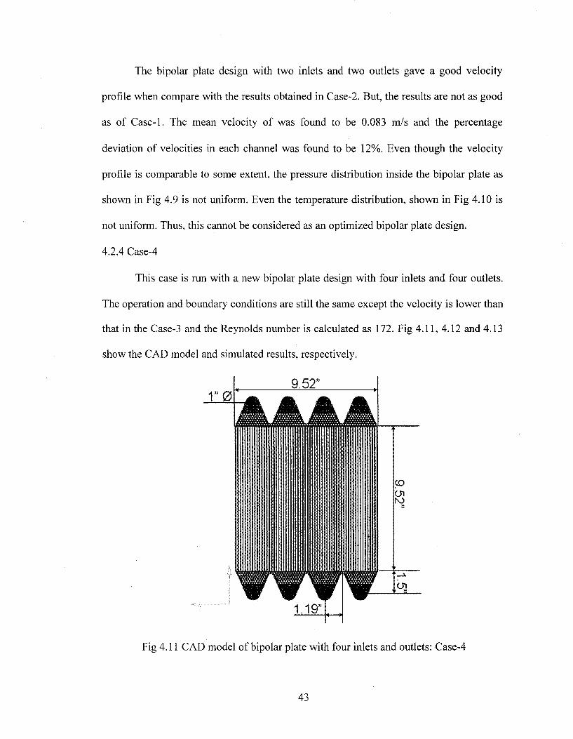
4.2.4 Case-4

This case is run with a new bipolar plate design with four inlets and four outlets.

The operation and boundary conditions are still the same except the velocity is lower than

that in the Case-3 and the Reynolds number is calculated as 172. Fig 4.11, 4.12 and 4.13

show the CAD model and simulated results, respectively.

1"09 . 5 2 "

1 . 19 ”

CDcnto

cm

Fig 4.11 CAD model o f bipolar plate with four inlets and outlets: Case-4

43

1.4

1.2

üTO-S

E^ Z o 6

0.4

0.2

0.1

N

- 0.1

-D.2

1,1

J I 1 I I I I L0.1 0.2

Pressure (Pa)105100959085807570856055504540353025201510

0.3

hiiiiiiiiiiiiiiiiitiiiiiiiiiiiiimuiiiminmimiiiiii0.05 0.1 0.15

X ( m )0.2

Fig 4.12 Velocity distribution plot and pressure contour; Case-4

Temperature (k)

' 1 , 1, «

357356.8356.6356.4356.2 356355.8355.6355.4355.2 355354.8354.6354.4354.2 354353.8353.6353.4353.2

Fig 4.13 Temperature contour: Case-4

44

The velocity profile obtained in this is very similar to that obtained in Case-1 with

6 inlets and 6 outlets. Even though the pressure distribution inside the bipolar plate is

slightly non-uniform, it is comparable with that obtained in Case-1. The mean velocity o f

was found to be 0.083 m/s and the percentage deviation o f velocities in each channel was

found to be 4.58%. The temperature contour is also uniform, and the temperature rise is

also similar to Case-1.

4.3 Conclusion

From the above four eases it is found out that the bipolar plate design with 1 and 2

inlets are not good designs and that with 6 inlets and outlets gives very good results. The

bipolar plate design with 4 inlets and 4 outlets also gives good results and these results

are very much similar to those obtained for 6 inlets. Thus one o f these two has to be

chosen as an optimized design and will be used for further analysis. Taking material

usage for the manufacturing o f the bipolar plate and the manufacturing costs, it can be

said that bipolar plate with 4 inlets and outlets is the optimized design. This design uses

less material when compared with bipolar plate with 6 inlets and outlets. Thus the bipolar

plate with 4 inlets and 4 outlets will be used for further analysis.

In the next chapter, the new optimized bipolar plate which was selected earlier

will be simulated to study the flow distribution inside the channels with multi-phase flow.

45

CHAPTER 5

HYDRODYNAMIC ANALYSIS ON TW O-PHASE FLOW

5.1 Need for Two-Phase Flow Analysis

In the previous chapters, the fluid flow inside the bipolar plate was discussed and

the model was developed which gave uniform flow and temperature distribution. For this

kind o f analysis water was used as the fluid that flowed through the plate. But, in reality,

the water flows through the inlet ducts and enters the channels and there it is split into

hydrogen ions (H^) and hydroxide ions (OH ) when it comes in contact with the bottom

surface o f the bipolar plate where constant heat flux is supplied. Then, the reduction

reaction occurs and the hydroxide ions combine with electrons and give water and

oxygen gas. This chemical equation was shown earlier in Chapter 1. Then the hydrogen

ions flow through the gas diffusion layer (GDL) and membrane electrode assembly

(MEA) and then enter another bipolar plate the other side. During entering another plate

it gains electrons from the cathode and becomes hydrogen gas.

In the first bipolar plate, where water is split, the remaining amount o f water

which is not split flows out o f the bipolar plate along with the oxygen gas produced. Thus

there is a two-phase flow inside the channels. The oxygen bubbles might result in non-

uniform flow inside the channels. Thus hydrodynamic analysis for two-phase flow must

46

be done to make sure that the new bipolar plate gives uniform flow. I f it does not give

uniform flow distribution, a new geometry must be developed. This chapter briefly gives

the introduction to two phase flow and discusses about whieh approach to follow,

assumptions made and finally the simulation and results.

5.2 Introduction to Two-Phase Flow

There are currently two approaches for the numerical calculation o f two-phase

flow:

1. Euler-Lagrange approach

2. Euler-Euler approach

In Euler-Lagrange approach, the fluid phase is treated as a continuum by solving

the time-averaged Navier-Stokes equations, while the dispersed phase is solved by

tracking a large number o f particles, bubbles or droplets through the calculated flow field.

The dispersed phase can exchange momentum, mass and energy with the fluid phase. In

this approach, the fundamental assumption made is that the dispersed second phase

occupies a low volume fraction. Thus, this approach is inappropriate for the models

where volume fraction o f the second phase is not negligible. In the current model, the

second phase is oxygen and its volume o f fraction is not neglected. Thus this approach is

inappropriate for the current experiment.

In Euler-Euler approach, the different phases are treated mathematically as

interpenetrating continua. Since the volume o f a phase cannot be occupied by the other

phase, the concept o f phasic volume fraction is introduced. These volume fractions are

assumed to be continuous functions o f space and time and their sum is equal to one. In

47

the commereial software FLUENT that is being used for the simulation, three different

Euler-Euler models are available;

1. The volume o f fluid model (VOF Model)

2. The Eulerian model

3. The mixture model

VOF model is a surface-tracking technique applied to a fixed Eulerian mesh. It is

designed for two or more immiscible fluids where the position o f the interface between

the fluids o f interest. The Eulerian model is the most complex o f the multiphase models

in FLUENT. Two-phase flow analysis with this model take more computational time

than the other models and streamwise periodic flow with specified mass flow rate cannot

be modeled when the Eulerian model is used. The mixture model is designed for two or

more phases. As in the Eulerian model, the phases are treated as interpenetrating

continua. The mixture model solves for the mixture momentum equation and prescribes

relative velocities to describe the dispersed phases. This model can be used for bubbly

flows. It can also be used without relative velocities for the dispersed phases to model

homogeneous multiphase flow.

For the current model analysis, mixture model theory is used. The new design is

run only for hydrodynamic analysis. It is not solved for the energy equation. The new

governing equations for continuity and momentum equations are

48

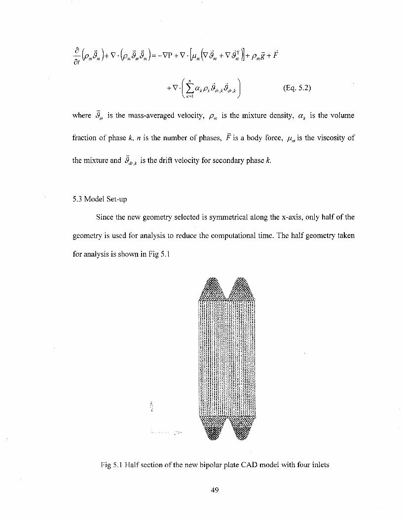
et

+v- dr,k\ A--1

(Eq. 5.2)

where 3,„ is the mass-averaged velocity, p„, is the mixture density, or* is the volume

fraction o f phase k, n is the number o f phases, F is a body force, is the viscosity o f

the mixture and ,9 ^ is the drift velocity for secondary phase k.

5.3 Model Set-up

Since the new geometry selected is symmetrical along the x-axis, only half o f the

geometry is used for analysis to reduce the computational time. The half geometry taken

for analysis is shown in Fig 5.1

Fig 5.1 Flalf section o f the new bipolar plate CAD model with four inlets

49

The operating conditions are the same as considered for the flow and temperature

distribution analysis in the previous chapter. In the boundary conditions, since the energy

equation is not solved, heat flux is not defined at the bottom walls o f the channels. Sinee

the number o f inlets is reduced to 2, the mass flow rate is also halved (0.15 1pm). In this

experiment, water is split to hydroxide ions and hydrogen ions inside the channels as

mentioned earlier. But, since the chemical reaction is not considered in this part o f the

analysis, it is assumed that oxygen is supplied from the bottom o f the ehannels, where

earlier, the heat flux was defined. The mass flow rate o f the oxygen supplied is given as

0.012 g/s. This value is given by Proton Energy Systems.

5.4 Results and Parametric Study

5.4.1 Case-1

This case is run with the operating conditions and the boundary conditions

mentioned in the previous section. After simulation, the velocity profile o f the water

inside the channels is plotted and is shown in Fig 5.2. The slice taken at the same location

as discussed in the previous chapters.

From the plot shown below, it can be found that even for two phase flow analysis,

the bipolar plate designed gives uniform flow distribution. Thus it can be accepted as an

optimized design o f the bipolar plate for the PEM electrolysis cell. But, before that

parametric study is carried out by varying the mass flow rate o f the oxygen and water

supplied. The results o f these cases are shown in the following sections as different cases.

50

0 . 6

0.5

w 0.4Ego 0.3 0 )>N

0.2

Operating Conditions:

R e = 172

Volumetric flow rate o f HiO = 0.3 1pm

Mass flow rate o f O2 = 0.012 g/s

Fig 5.2 Velocity profile for two-phase flow

5.4.2 Case-2

In this case the volumetric flow rate o f the water is unchanged but the mass flow

rate o f the oxygen is reduced to 0.01 g/s. All other operating conditions and boundary

conditions are unchanged. The model is then run and the velocity profile o f water inside

the ehannels is plotted. The velocity profile is shown in Fig 5.3. When the velocity profile

o f Case-2 is compared with that o f Case-1, not much difference is observed. The velocity

profile is still uniform inside the channels.

51

0.6

0.5

-w 0.4 E' So 0.30 )>

0.2

Operating Conditions;

Re= 172

Volumetric flow rate o f H 2 O = 0.3 1pm

Mass flow rate o f O2 = 0.01 g/s

0.02 0.04 0.06 0.08X(m)

0.1 0.12

Fig 5.3 Velocity Profile for 0.3 1pm Water and 0.010 g/s Oxygen

5.4.3 Case-3

In this case, the volumetric flow rate o f the water is increased to 1.5 1pm so as to

observe the behavior o f water for high flow rates. The mass flow rate o f the oxygen is

assumed to be increased linearly and increased to 0.06 g/s. The velocity profile o f this

case is shown in Fig 5.4

52

Operating Conditions:

0.9 Re = 859

Volumetric flow rate o f H2O = 1.5 1pm0.8

Mass flow rate o f O2 = 0.06 g/s0.7

E 0.6

f o . 50

^ Q A1

N0.3

0.2

0.120.02 0.04 0.06X( m)

0.08

Fig 5.4 Velocity profile for 1.5 1pm o f water and 0.06 g/s oxygen

As the volumetric flow rate o f the water increased from 0.3 1pm to 1.5 1pm, it is

found that there is a small non homogeneity in the flow distribution inside the channels.

But, the percentage error in the uniformity is not very high (5%) and this can be still

accepted as an optimized design.

5.5 Validation

The basic bipolar plate and the new bipolar plate designed were simulated

numerically and by plotting the results it was found that the new bipolar plate design

53

gives us uniform flow and temperature distribution inside the charmels. Before accepting

these numerical results, it should be validated that the results obtained from the numerical

analysis are reasonable with the analytical calculations. For this, back-of-the-envelope

calculations are to be done and compared with the numerical results.

In this experiment, to validate the results obtained, the volume fraction o f the

oxygen is calculated at the outlet and then it is compared with the numerical results. I f the

calculated value is comparable with the results obtained by the numerical analysis, then

the experiment is said to be validated and the model can be used. The percentage o f

volume fraction o f oxygen is calculated by

VOF = ----------------- *100Q oxy^cn Qwafer

where is the volumetric flow rate o f oxygen and the is the volumetric flow

rate o f the water at the respective inlets.

From the results obtained from the numerical analysis, the VOF o f oxygen at the

outlet is plot for all the three cases and are shown in Figs 5.5, 5.6 and 5.7, respectively.

And the comparisons between numerical and analytical values are shown in Table 5.5-1.

54

X

VOF Oxygen

■ 0 . 7

0.69 0.68 0.67 0.66 0.65 0.64 0.63 0.62 0.61 0.6 0.59 0.58 0.57 0.56 0.55

Fig 5.5 VOF o f oxygen at outlet in case-1

VOF Oxygen

I

Fig 5.6 VOF o f oxygen at outlet in case-2

55

X

VOF Oxygen

10.7 0.69 0.68 0.67 0.66 0.65 0.64 0.63 0.62 0.61 0.6 0.59 0.58 0.57 0.560.55

Fig 5.7 VOF o f oxygen at outlet in case-3

fable 5.5-1 Comparison between numerical and analytical results

Case

No.

Description Numerical

Result (%)

Analytical Results

(%)

1 Mass flow rate o f oxygen = 0.012 g/s;

Volumetric flow rate o f water = 0.3 1pm

62.8 - 69.6 64.8

2 Mass flow rate o f oxygen = 0.010 g/s;

Volumetric flow rate o f water = 0.3 1pm

5 9 - 6 5 .4 60.6

3 Mass flow rate o f oxygen = 0.06 g/s;

Volumetric flow rate o f water = 1.5 1pm

64 — 65.7 64.8

56

From the above table, it can be found that the values obtained by the numerical

analysis are close to the analytical values. The percentage error between both the values

is not more than 5%. Hence, the values obtained from the numerical analysis are

acceptable.

57

CHAPTER 6

CONCLUSIONS AND FUTURE WORK RECOMMENDATIONS

6.1 Conclusions

Numerical modeling has been performed to study the flow and temperature

distribution inside the bipolar plate o f PEM electrolysis cell in this thesis. The

conclusions pertaining to this research work are summarized as follows

• The basic bipolar plate design which was given by Proton Energy Systems USA,

was simulated and was found that the flow distribution inside the charmels in not

uniform. This is because; the flow o f the water inside the header, after exiting the

inlet duct charmels is almost in the perpendicular direction to the charmels. Thus

the flow through the end charmels is more when compared with the middle

charmels.

• This problem is solved by designing new bipolar plates to which the inlet and

outlet ducts are cormected in such a way that the flow direction o f the water which

enters the header from the ducts is almost parallel to the charmels. With this kind

o f design, uniform flow and temperature distributions are achieved inside the

bipolar plate.

• The new bipolar plate design was then simulated for two-phase hydrodynamic

flow analysis. The results gave little non-uniformity for higher mass flow rates o f

58

water and oxygen. But, since the percentage o f non-uniformity is significantly less, it can

be accepted as the good design o f the bipolar plate.

6.2 Future Recommendations

The current experiment resulted in the design o f a new bipolar plate which gives

uniform flow and temperature distributions. But, there were several assumptions made to

achieve these approximate results. To achieve better results and to study the design o f the

bipolar plate more accurately, few modifications have to be made in the simulations and

few other simulations must also be performed which might give better results. Some o f

them are mentioned below

• In two-phase flow analysis, the model was simulated only for continuity and

momentum equations. It should be simulated for the energy equation also.

• In a bipolar plate o f the PEM electrolysis, the water is split into hydrogen ions and

hydroxide ions and later the hydroxide ions give oxygen gas and water due to

reduction reaction. In current two phase flow analysis, it was assumed that the

oxygen is supplied from the bottom walls o f the channels. Numerical analysis

with a chemical reaction defined at the surface will give much realistic solutions.

• It was also assumed that the oxygen is supplied uniformly along those bottom

surfaces where as in reality; the oxygen generation might not be uniform along

the surface. So, the two phase flow analysis must be done with a user defined

function to define the generation o f oxygen inside the plate.

• In the current numerical experiment, the escape o f the hydrogen ions from the

bipolar plate into the gas diffusion layer was not studied. So, simulation o f the

59

complete PEM assembly must be carried out to see the actual behavior o f water,

oxygen and hydrogen ions inside the bipolar plate.

No experimental work has been done on the current PEM electrolysis cell. The

experimental results will help in validating the results obtained from the

numerical simulations performed, more accurately. So, a real time experiment

must be carried out to know the exact behavior o f each component in the cell.

60

REFERENCES

1 . www.effectofglobalwarming.com

2. Pearson, Paul N.; Palmer, Martin R. (2000-08-17). "Atmospheric Carbon Dioxide

Concentrations over the Past 60 M illion Years". Nature 406 (6797): 695-699.

3. Marland, G., T.A. Boden, and R. J. Andres. 2007. Global, Regional, and National

C 02 Emissions. A Compendium of Data on Global Change. Carbon Dioxide

Information Analysis Center, Oak Ridge National Laboratory, United States

Department o f Energy, Oak Ridge, Term., U.S.A.

4. http://usinfo.state.gov/products/pubs/economy-in-brief/pagel 1 .html

5. http://www.thenation.eom/doc/20071112/klare

6 . http://www.worldwatch.org/fdes/pdf/renewables2007.pdf. Renewable 2007 Global

Status Report.

7. http://www.worldofrenewables.com/page.php?pageid=48

8 . http://www.pege.org/greenwinds/electrolyzer.htm

9. loannis Papagiannakis, “Studying and Improving the Efficiency o f W ater Electrolysis

using a Proton Exchange Membrane Electrolyzer” , MS Thesis, Strathclyde

University, 2005.

10. http://www.eoearth.org/article/Hydrogen_production_technology

11. Shanthi P. Katukota, “Computational Modeling o f Proton Exchange Membrane

Electrolysis Cell for Hydrogen Production”, MS Thesis, University o f Nevada Las

Vegas, 2006.

61

12. Hung Yue, El- Khatib K. M., Tawfik Hazem., “Corrosion-resistant light weight

metallic bipolar plates for PEM fuel cells,” Journal o f Applied Electrochemistry, Vol.

35, 445-447, 2005.

13. J. Divisek, “Water electrolysis in low and medium temperature regime”,

electrochemical hydrogen technologies, 137, 1990.

14. Barbir P., “PEM electrolysis for production o f hydrogen from renewable energy

sources,” Solar Energy, 78, 661-669, 2005.

15. Grigoriev S.A., Porembsky V.I., Fateev V.N., “Pure hydrogen production by PEM

electrolysis for hydrogen energy,” International Journal o f Hydrogen Energy, 31,

171-175,2006.

16. Choi P., Bessarabov D.G., Datta, R., “A simple model for solid polymer electrolyte

(SPE) water electrolysis,” Solid State Ionics, 175, 535-539, 2004.

17. Balster J., Stamatialis D.F., Wessling M., “Electro-catalytic membrane reactors and

the development o f bipolar membrane technology,” Chemical Engineering and

Processing, 43 (9), 1115-1127, 2004.

IS. Farrauto R., Hwang S., Shore L., Ruettinger W., Lampert J., Giroux T., Liu Y.,

Ilinich O., “New material needs for hydrocarbon fuel processing: generating

hydrogen for the PEM fuel cell,” Armual Review o f Materials Research, 33, 1-27,

2003.

19. Marshall A., Borresen B., Hagen G., Tsypkin M., Tunold R., “ Hydrogen production

by advanced proton exchange membrane (PEM) water electrolysers-reduced energy

consumption by improved electrocatalysis,” Energy, 32, 431-436, 2007.

62

20. Millet P., Andolfatto F., Durand R., “Design and performance o f solid polymer

electrolyte water electrolyzer,” International Journal o f Hydrogen Energy, 21(2), 87-

93,1996.

21. Rasten E, Electrocatalysis in water electrolysis with solid polymer electrolyte, PhD

Dissertation, NTNU Trondheim, 2001.

22. Yamaguchi M, Yagiuchi K, Okisawa K, “R&D o f high performance solid polymer

electrolyte water electrolyzer in W E-Net,” Hydrogen Energy Progress XI,

Proceedings o f the World Hydrogen Energy Conference, 781-786, 1996.

23. Nagai M, Tazima H, Sakanishi A, Hisatome N, Ohkura S, “Development on solid

polymer electrolyte water electrolysis technology for high current density and energy

efficiency,” Hydrogen Energy Progress XI, Proceedings o f the World Hydrogen

Energy Conference, 825-830, 1996.

24. Yamaguchi M, Okisawa K, Nakanori T, “Development o f high performance solid

polymer electrolyte water electrolyzer in W E-NET,” Proceedings o f the 32"'*

Intersociety Energy Conversion Engineering Conference, I958-I965, 1997.

25. Yamaguchi M, Shinohara T, Taniguchi H, Nakanori T, Okisawa K, “Development o f

2500 cm^ solid polymer electrolyte water electrolyzer in W E-NET,” Hydrogen

Energy Progress XII, Proceeding o f the World Hydrogen Energy Conference, 747-

755,1998.

26. Grigorev S, Khaliullin M, Kuleshov N, Fateev V, “Electrolysis o f water in a system

with a solid polymer electrolyte at elevated pressure,” Russian Journal o f

Electrochemistry (Translation o f Electrokhimiya), 37, 819-822, 2001.

63

27. Ledjeff K, M ahlendorf F, Peinecke V, Heinzel A, “Development o f electrode

membrane units for the reversible polymer fuel cell (RSPFC),” Electrochimica Acta,

40,315-319,1995.

28. Millet P, “Water electrolysis using EME technology: electric potential distribution

inside a nafion membrane during electrolysis,” Electrochimica Acta, 2501-2506,

1994.

29. Stucki S, Menth A, “Proceedings o f the industrial water electrolysis”, (edited by

Srinivasan S, Salzano A and Landgrebe K) Electrochemical Society, Princeton, p.

180,1978.

30. McBreen J, “Voltammetric studies o f electrodes in contact with ionomeric

membranes,” Journal o f Electrochemical Society, 132, 1112-1116, 1985.

31. Zhou Y., Lin G., Shih A.J., Hu S.J., “A micro-scale model for predicting contact

resistance between bipolar plate and gas diffusion layer in PEM fuel cells,” Journal o f

Power Sources 163, 777-783, 2007.

32. Heinzel A., M ahlendorf F., Niemzig O., Kreuz C., “Injection moulded low cost

bipolar plates for PEM fuel cells,” Journal o f Power Sources, 131, 35-40, 2004.

33. Muller. A., Kauranen. P., Von Ganski.A., Hell. B., “Injection moulding o f graphite

composite bipolar plates,” Journal o f Power Sources, 154, 467-471, 2006.

34. Barreras F., Lozano A., Valino L., Marin C., Pascau A., “Flow distribution in a

bipolar plate o f a proton exchange membrane fuel cell: experiments and numerical

simulation studies,” Journal o f Power Sources, 144, 54-66, 2005.

64

35. Atul Kumar, Ramana G. Reddy, “Effect o f gas flow-field design in the bipolar/end

plates on the steady and transient state performance o f polymer electrolyte membrane

fuel cells,” Journal o f Power Sources, 155, pp. 264-271, 2006.

36. http://www.greencarcongress.com/hsub2sub/index.html

37. FLUENT, Inc., GAMBIT 2.2, U ser’s Guide, Lebanon, NH, USA, 2004.

65

VITA

Graduate College University o f Nevada Las Vegas

Kiran Mohan Veepuri

Address:1555 E Rochelle Ave, Apt# 147 Las Vegas, NV 89119

Degree:• Bachelor o f Engineering, Mechanical Engineering, 2005

Osmania University, India

Professional Experience:• Worked as Design Engineer at Wipro Technologies, Hyderabad, India, June ’05-

Dec ’06• Research Assistant, University o f Nevada Las Vegas, Jan ’07-Present

Thesis Title: Optimization o f Bipolar Plate Design for Flow and Temperature Distributions Using Numerical Techniques

Thesis Examination Committee:Chairperson, Dr. Yitung Chen, Ph.D.Committee Member, Dr. Robert F .Boehm, Ph.D.Committee Member, Dr. Jianhu Nie, Ph.D.Graduate College Representative, Dr. Rama Venkat, Ph.D.

66