Embed Size (px)
Citation preview

Journal of Industrial Engineering and ManagementJIEM, 2016 – 9(2): 374-388 – Online ISSN: 2013-0953 – Print ISSN: 2013-8423
http://dx.doi.org/10.3926/jiem.1929
Optimization of a Truck-drone in Tandem Delivery Network
Using K-means and Genetic Algorithm
Sergio Mourelo Ferrandez1 , Timothy Harbison1 , Troy Weber1 , Robert Sturges2 , Robert Rich2
1Liberty University (United States)2Virginia Tech University (United States)
[email protected], [email protected], [email protected], [email protected], [email protected]
Received: February 2016Accepted: April 2016
Abstract:
Purpose: The purpose of this paper is to investigate the effectiveness of implementing
unmanned aerial delivery vehicles in delivery networks. We investigate the notion of the reduced
overall delivery time and energy for a truck-drone network by comparing the in-tandem system
with a stand-alone delivery effort. The objectives are (1) to investigate the time and energy
associated to a truck-drone delivery network compared to standalone truck or drone, (2) to
propose an optimization algorithm that determines the optimal number of launch sites and
locations given delivery requirements, and drones per truck, (3) to develop mathematical
formulations for closed form estimations for the optimal number of launch locations and the
optimal total time of delivery.
Design/methodology/approach: The design of the algorithm herein computes the minimal
time of delivery utilizing K-means clustering to find launch locations, as well as a genetic
algorithm to solve the truck route as a traveling salesmen problem (TSP). The optimal solution is
determined by finding the minimum cost associated to the parabolic convex cost function. The
optimal min-cost is determined by finding the most efficient launch locations using K-means
algorithms to determine launch locations and a genetic algorithm to determine truck route
between those launch locations.
-374-

Journal of Industrial Engineering and Management – http://dx.doi.org/10.3926/jiem.1929
Findings: Results show improvements with in-tandem delivery efforts as opposed to standalone
systems. Further, multiple drones per truck are more optimal and contribute to savings in both
energy and time. For this, we sampled various initialization variables to derive closed form
mathematical solutions for the problem.
Originality/value: Ultimately, this provides the necessary analysis of an integrated truck-drone
delivery system which could be implemented by a company in order to maximize deliveries while
minimizing time and energy. Closed-form mathematical solutions can be used as close estimators
for the optimal number of launch locations and the optimal delivery time.
Keyword: evolutionary, K-means, truck drone in tandem delivery network, UAV
1. Introduction
The technology for UAVs and drones has increased significantly in the past few years, and the list of
potential uses for automated drones is growing annually across various disciplines. Conversely, there has
been limited research in the area of systems level planning and execution for a network of drones within a
given environment.
The problem herein examines a truck-drone team from an operational viewpoint to better understand the
impact of the number and location of truck stops with regards to its effect on delivery time and energy
requirements. Initially, we analyze a single drone to deliver all packages to all locations. This requires one
truck stop centrally positioned among the delivery locations using K-means. The drone uses a hub
configuration to egress and ingress from the truck to each delivery location and back, not constrained by
range. We intend to understand the total time, cost, and energy involved in a hub configuration
(star-distance) in order to contrast this configuration with truck-only delivery using a TSP route. We use a
genetic algorithm to compute this TSP truck route in order to satisfy all the deliveries to all the locations.
Furthermore, we use a combination of truck and drone to find the optimal number of truck stops and
locations using K-means algorithm to cluster demands in conjunction with a TSP genetic algorithm.
The problem herein assumes that one or more drones and a single truck work in tandem to deliver
packages to delivery locations within a given delivery space; and that the uniformly distributed delivery
demands are known a priori. The drones are not constrained by range to gain a better sense of the
upper/lower boundaries of time and energy. Further, neither the truck nor the drone is constrained by a
system of roads but each type vehicle can move directly to any delivery location as required. However, the
truck is constrained to move along a TSP route while the drone is constrained to egress and ingress from
-375-

Journal of Industrial Engineering and Management – http://dx.doi.org/10.3926/jiem.1929
the truck in hub (star) configuration to a nearby delivery location and then back to the truck. A truck stop
denotes the following: (1) a delivery location of one package from the truck and (2) a launch location for
the drone to deliver one package to each nearby delivery location associated to that truck stop by means
of K-MEANS clustering.
2. Similar Existing Models in Literature
Danzig and Ramser investigated the vehicle routing problem (VRP) wherein they described a delivery
scenario of fuel to gas stations whereby integer programming and other algorithmic approaches were
utilized to solve the problem (Dantzi & Ramser, 1959). Later, Clarke and Wright proposed an effective
greedy heuristic which was subsequently followed by several models involving exact and heuristic
approaches to solve the variations of the VRP (Clarke & Wright, 1964). An extensive survey was
conducted by Desrochers, Lenstra, and Savelsbergh devoted to formulating exact methods of solving the
VRP and provided an overview of the system state (Desrochers, Lenstra & Savelsbergh, 1990).
Drone research today involves a number of papers on various topics from obstacle detection-avoidance,
GPS enhancements, hijacking, endurance, and navigation. However, from an operational standpoint, only
a handful of papers deal with the operational aspects of a package delivery system. One recent publication
was written by Chen and MacDonald describing a set of nodes and drones interconnected by a delivery
network interrupted by the random arrival of packages at any node. The objective was to discuss how to
plan and solve for the number of drones given the demands on the system. A simulation model was
recommended for the problem due to the stochastic nature of the scenario (Chen & MacDonald, 2014).
In another recent paper, Murray and Chu formulated an optimization parcel delivery problem using
trucks and drones. They determined the optimal routing of the truck-drone as synergistic agents in the
delivery effort, such that the total delivery time was minimized. For their case, the truck serves to launch
the drone from an efficient launch location prior to reaching the ‘last mile’ of the delivery effort. A multi-
integer programming (MIP) solution is formulated to solve the problem (Murray & Chu, 2015).
3. Proposed Optimization Model
The optimization algorithm herein utilizes a hybrid Newton’s method with difference equations. This
employs a cost function (J) to solve for the optimal delivery time and associated number of centroids.
Inputs to the optimization function include a set of delivery coordinate locations (P) whereby the length
of this parameter denotes the number of customers (kup).This upper boundary (kup) represents a truck
only delivery while Klow represents a drone only delivery solution. For non-convex functions, a truck only
-376-

Journal of Industrial Engineering and Management – http://dx.doi.org/10.3926/jiem.1929
solution is optimal. Otherwise, the optimal delivery time (bestTime) for the in tandem system is a function
of speed of the truck (Ts), speed of the drone (Ds), number of drones per truck (dr), as well as the number
(kup) of deliveries and their respective locations (P).
3.1. Optimization Function
Algorithm 1: Optimization algorithm (hybrid Newton’s method)
Function Optimize(P)Input
P = {p1, p2, …, pn}; (Set of customer delivery locations to be clustered)kup (Total number of customers or size n of P)dr (Number of drones per truck)
Output:bestTime (Optimal time in hours to delivery)optimalK (Optimal number of stops (centroids))
InitializebestTime = Infinity;optimalK = kup;
Ts = 35 truck speed ;
Ds = Ts*1.5 (drone speed ); (Drone speed a factor of truck speed in km/h)
klow = 2; (Min number of calculable centroids or stops)K = {klow, klow +10, kup-10, kup} (k centroids for test for convexity)Convex = ArgCheckConvex(P, K, ts, ds);α = 10; (Learning rate for hybrid Newton's Method 2 to 15)if not Convex then
return;end
K1 = ; (Initialize K)
J1 = CostFunction(K1, P, Ts, Ds, dr); (Initialize J)foreach 1:MaxItr do (for loop)
Ki+1 := Ki – ag; (Gradient descent using learning rate alpha)Ji+1 := CostFunction( Ki+1, P, Ts, Ds, dr); (Call to cost function)dJi := Ji+1 – Ji; (Change in cost function)dKi := Ki+1 – Ki; (Change in K centroids)
g := ; Gradient of cost function with respect to change in centroids)
if Ji+1 < bestTime thenbestTime := Ji+1; (Captures the best time)optimalK := Ki+1; (Captures the K centroids based on best time)
endendreturn bestTime, optimalK
-377-

Journal of Industrial Engineering and Management – http://dx.doi.org/10.3926/jiem.1929
3.2. Cost Function
The cost function utilizes the number of centroid stops (K) to evaluate total time. Once initialized, the
function calls the KMEANS algorithm to calculate the K optimal centroids locations (C) based on
customer locations (P). KMEANS returns both optimal location and star distance between customer
locations and centroid locations. Star distance (sD) is the mathematical representation for drone ingress
and egress in hub configuration from truck to customer and back to truck. The KMEANS returned
centroid locations (C) are used by the genetic algorithm to calculate truck route (R) defined as the
minimum route of the traveling salesman problem. The genetic algorithm returns both the optimal truck
route and the minimum truck route distance (tD). Both truck distance (tD) and sum of all drone star
distances (sumD) are divided by their respective vehicle speeds to determine the total time required for (K)
truck stops. The total time required for (K) truck stops is returned as the cost function.
Algorithm 2: Cost Function
CostFunction (K, P, Ts, Ds, dr)Input
Ds (Drone speed )
Ts (Truck speed )
k (Number of centroids or stops)P = {p1, p2, …, pn}; (Set of customer locations)dr (Number of drones per truck)
Output:totTi (Total time resulting from K stops)
Initialize:MaxIter =3 (Maximum number of iterations used to average total time)
foreach 1:MaxItr do (for loop)C, L, sD := CallKmeans(K, P); (Kmeans returns centroid location, distance, and labels)
; (Sum of star distances multiplied by 2m ingress egress)
R, tD := CallGenetic(K,C); (Returns TSP route and min TSP distance)
; (Total time at each iteration based on vehicle speeds)
end
; (average the total times at each iteration for convergence)
end
-378-

Journal of Industrial Engineering and Management – http://dx.doi.org/10.3926/jiem.1929
3.3. K-Means Algorithm
The generalized KMEANS algorithm as described by (MacQueen, 1967) simply partitions n objects into
(K) clusters were each object is associated with closest cluster center. It clusters the delivery location into
k-groups where k, or the number of centroids is pre-defined. KMEANS herein utilizes the KMEANS
(MathWorks, 2013) two phase operation to solve for least distance between points (delivery locations) to
nearest centroid (truck launch) summed over all K clusters based on concepts described in works by
Seber (1984) and Spath (1985). The first phase assigns delivery locations to the nearest cluster (centroid)
all at once and then re-calculates the centroids. Phase I typically results in a sub-optimal local minimum,
but gives good candidate centroids for initialization and Phase II. The second phase utilizes ‘on-line’
updates whereby candidate points are reassigned to different centroids if the act of reassignment reduces
the cost. KMEANS algorithm herein is adapted from Seber (1984) and Spath (1985).
Algorithm 3: Cost Function
Function CallKmeans(k,P)Input
P = {p1, p2, …, pn}; (Set of customer to be clustered to centroids)k (Number of centroids)
Output:C = {c1, c2, c3, …, ck}; (Set of calculated centroids)L = {l(p) | p = 1, 2,…, n}; (Set of cluster labels for Customer p)D = {d(p) | p = 1, 2,…, n}; (Set of cluster distances for Customer p)
foreach ci C do (for loop)
ci := pj P; (Initial cluster assignment according to Phase I)end
foreach pi P do (for loop)
l(pi) := ArgMinDistance(pi, cj) where j {1...k}; (Assigns customer to closest centroid)endchanged := false; (Flag to stop repeat)iter := 0; (Count iteration in repeat)repeat (outer while loop)
foreach ci C do (inner for loop)UpdateCluster(ci); (Based on Phase II)end
foreach ei P do (inner for loop)
minDist := ArgMinDistance(pi, cj) where j {1...k}; (Find Minimum distance)if minDist ≠ l(pi) thenl(pi) := minDist; (Capture Minimum distance)changed := true;end
enduntil changed == true and iter ≤ MaxIter
-379-

Journal of Industrial Engineering and Management – http://dx.doi.org/10.3926/jiem.1929
3.4. Genetic Algorithm
The genetic algorithm herein is adapted from Joseph Kirk (2007). This efficient algorithm randomly
permutes 200 routes finding a route with best distance within this population. The algorithm begins by
permuting a given population of potential route sequences. It randomly selects a number of routes and
finds the best from this selection. Once the best route is found, it mutates the route in five efficient ways
thus creating a new route for each mutation. Mutations are: (1) reverse orders a short segment within the
route from randomly selected points A to B; (2) reverse orders a short segment within the route from
randomly selected points B to C; (3) Slide a route segment B to C one space left, then replaces the last
element B with the first element A; (4) in route segment A, B, it swaps centroids A and B; and (5) keeps
the original best route. The entire population is updated based on random variations of the five mutations
of the best route. The efficient algorithm solves for large TSP (n>200) problems in relatively short time
(i.e. less than two minutes).
Algorithm 4: Genetic Algorithm
Function CallGenetic(k, C)Input
C = {c1, c2, c3, …, ck}; (Set of centroids results from CallKmeans to be TSP routed)n = k where (k>2)
Output:optimalRoute = {r1, r2, r3, …, rn}; (TSP route sequences from 1 to n)globalMinDist; (Calculated min distance for optimal route)
Initializep:=200; (Population size)POPpn := ArgRandPermute(p,n); (Randomly Permute route sequence matrix)DISTij := ArgEuclideanDistance(ci, cj); (Square distance matrix between centroids)globalMinDist := infinity;MaxIter := round(25n9); (Maxiterations based on route size)
foreach 1 to MaxIter do (outer for loop)minDist, index = ArgMinPathDist(POPpn, DISTij); (Find min distance route in population)
if minDist<globalMinDist thenglobalMinDist:=minDist; (Capture Minimum Distance)optimalRoute:= POPindex, :; (Capture Best Route)end
rPOP5,n := ArgRandSelect(POP); (omly select five routes from population)minDist, index = ArgMinPathDist(rPOP5,n, DISTij); (Find min distance of the five routes)rShuff1:n := randShuffle(1:n); (Random shuffle 1:n integers)rand1, rand2 := sort(rShuff1,2); (Take two elements (A,B) of random shuffle, sort)rand2, rand3 := sort(rShuff2,3); (Take two elements (B,C) of random shuffle, sort)foreach k in 1 to 5 do
-380-

Journal of Industrial Engineering and Management – http://dx.doi.org/10.3926/jiem.1929
tmpPOP5,n := getBestRoute(index); (Get the best of five routes for mutation)switch kcase 2 (Reverse order a random route segement in best sequence A to B)
tmpPOP(k, rand1 :rand2) = tempPOP(k, rand1 :-1 :rand2);case 3 (Reverse order a random route segement in best sequence B to C)
tmpPOP(k, rand2 :rand3) = tempPOP(k, rand2 :-1 :rand3);case 4 (Slide a route segment B to C, replace last element with first element)
tmpPOP(k, rand2 :rand3) = tempPOP(k, [rand2 +1 :rand3 rand2]);case 5 (Swap two centroids in route sequence A to B)
tmpPOP(k, [rand1 rand2) = tempPOP(k, [rand2 rand1])otherwise
do nothing;endnewPop(p-3:p,:) := tmpPOP; (Update new population with the mutations of best)endpop := newPop; (Set population as new population)end
4. Closed Form Mathematical Solutions (Estimations)
Data generated from the optimization algorithms of typical discretized state space initialization variables,
various drone speeds, truck speeds, number of deliveries, and drones per truck was used to formulate
closed form estimations for the number of stops and total delivery time, given input parameters. The
following closed form solutions gave good estimates for expected delivery time and number of truck
stops for uniformly distributed demands. Using ANOVA, each of the input variables were analyzed to
find the significance of the input variables to the output variable. In each case, the input variables revealed
a significant impact on the output as shown by low p-values (i.e. 3×10-16). Estimated number of centroids
(truck route stops/launches) and the estimated delivery time was found to be a function of size of
delivery area, truck speed (Ts), drone speed (Ds), number of drones (dr), and number of deliveries
(totCust).
4.1. Optimal K and Time Function (Uniform Distribution)
The state space was discretized as shown in Table 1 below. Truck speed was held constant at 35 km/h
while the drone speed was investigated starting at 35 km/h, then incremented by 17.5 km/h to a max
speed of 105 km/h denoted by 35:17.5:105. The optimal time and optimal number of truck stops was
found for each unique set of input initialization values. In all, 1,600 initialization parameters were
analyzed, and the optimization algorithms produced optimal values for total delivery time and number of
-381-

Journal of Industrial Engineering and Management – http://dx.doi.org/10.3926/jiem.1929
stops for each case. This dataset, comprised of inputs and optimal outputs, was then used to formulate
closed form estimates.
Factor Levels Total Levels
Truck Speed 35 1
Drone Speed 35: 17.5: 105 5
No. Drones 1, 2, 3, 4 4
No. Customers 50:50:250 5
Operating Space Uniform Dist. (25: 25: 200) 8
Model MATLAB™ 1
Total Problem Instances 2 Replications (5*4*5*8*2) 1,600
Table 1. Discretized state space initialization parameters
4.1.1. Optimal K (Number of Truck Stops to Launch Drones)
(1)
Equation (1) represents the number of K-clusters, or more specifically the optimal number of truck stops,
given the input variables.
Figure 1. Power function Y = C Xa where
-382-
Journal of Industrial Engineering and Management – http://dx.doi.org/10.3926/jiem.1929
The goodness of fit of this function is high as the adjusted R – square is 0.9011, and therefore, it can be
used for estimating the optimal number of clusters (Optimal K) of this system.
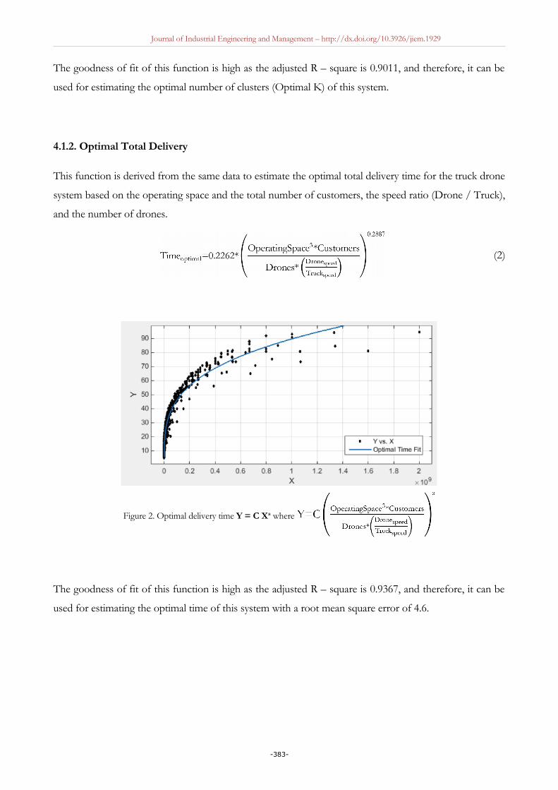
4.1.2. Optimal Total Delivery
This function is derived from the same data to estimate the optimal total delivery time for the truck drone
system based on the operating space and the total number of customers, the speed ratio (Drone / Truck),
and the number of drones.
(2)
Figure 2. Optimal delivery time Y = C Xa where
The goodness of fit of this function is high as the adjusted R – square is 0.9367, and therefore, it can be
used for estimating the optimal time of this system with a root mean square error of 4.6.
-383-

Journal of Industrial Engineering and Management – http://dx.doi.org/10.3926/jiem.1929
5. Experimental Results
Experiments were conducted on various inputs of state space to gain a sense of the variations in
optimal solutions compared to various distributions as well as performance criteria. Performance
criteria analyzed included total delivery time, total energy used, and total costs based on cost per km
and cost per hour.
5.1. Optimal Time Analysis
As shown in Table 2, the resultant delivery time cost curve is depicted as a parabolic, convex and
quasi-continuous cost function. The delivery time graph was created by analyzing brute force 2 to 100 truck
stops (2:2:100). We see that two truck stops is not optimal. On the other end of the abscissa, we see that
the truck performing all the stops (i.e. abscissa value 100), that this too was not optimal. The optimal
solution was found utilizing both truck and drone, a value between the two extremes.
Optimal Time (ordinate) and Number of truck stops (abscissa)
Initialization Parameters Simulation (Brute Force)
Operating Space Size 100 km by 100 km
Customers (100) deliveries (uniformlydistributed)
Truck speed km/h (35)
Drone speed km/h (70)
Number of Drones per truck (2)
Uniformly distributed demand
Optimal Results:Optimality found at
Stops: 22 stopsDelivery Time: 27 h
Table 2. Optimal Time Analysis
-384-

Journal of Industrial Engineering and Management – http://dx.doi.org/10.3926/jiem.1929
5.2. Energy Estimates of in Tandem System
Rough energy estimates are given to understand the differences in energy requirements between trucks
and drones based on uniformly distributed demand delivery requirements. For these high level estimates a
few assumptions are provided. A drone is assumed to require 448 Watts per second (Allain, 2013) at
100% efficiency; and if we assume 50% efficiency of the drone rotor system, then the drone requires 896
Watts (896 Joules per second) when in flight. Thus, the drone is estimated here to fly at 70km/h and
deliver to each customer in the star configuration associated to each of the cluster centroids. Since our
resulting time for experiments is in hours, the energy required for drones (Edrone) is multiplied by 3,600 and
then the number of hours required for total drone delivery.
The truck’s estimated speed is 35 km/h and is tasked to circumnavigate each of the centroids in a TSP
route configuration. The truck is estimated get 10 miles / gallon of diesel; and each gallon of diesel has
approximately 1.3×10⁸ J of energy. The algorithm computes a TSP truck route in kilometers
(total_TSP_truck_route) for each of the possible centroids. The energy requirements for the truck (Etruck)
calculation is based on the TSP route converted to miles and then multiplied by Joules per gallon of diesel
fuel.
We analyzed the total energy requirements for each of the possible centroids in our experiments. These
ranged from 2 to 100 centroids to determine the optimal energy expenditure. Energy requirements for
truck and drone were added to give the total energy requirements per each centroid configuration. Results
showed that the least amount of energy would be expended if the drone delivered each of the packages
even though both ingress and egress routes would have to be traversed which resulted in more than twice
the distance. It is assumed that these efficiencies are due to four general principles: (1) efficiencies of the
brushless rotor are higher than those of the diesel engine, (2) the load to vehicle weight ratios is
significantly different for each vehicle and impacts efficiencies, (3) reduced friction efficiencies found in
air transport generally outweigh energy loss due to mechanical/tire friction, and (4) systems that are
cooler tend to use less energy as the drone’s brushless motors will run significantly cooler than the truck’s
diesel engine.
-385-
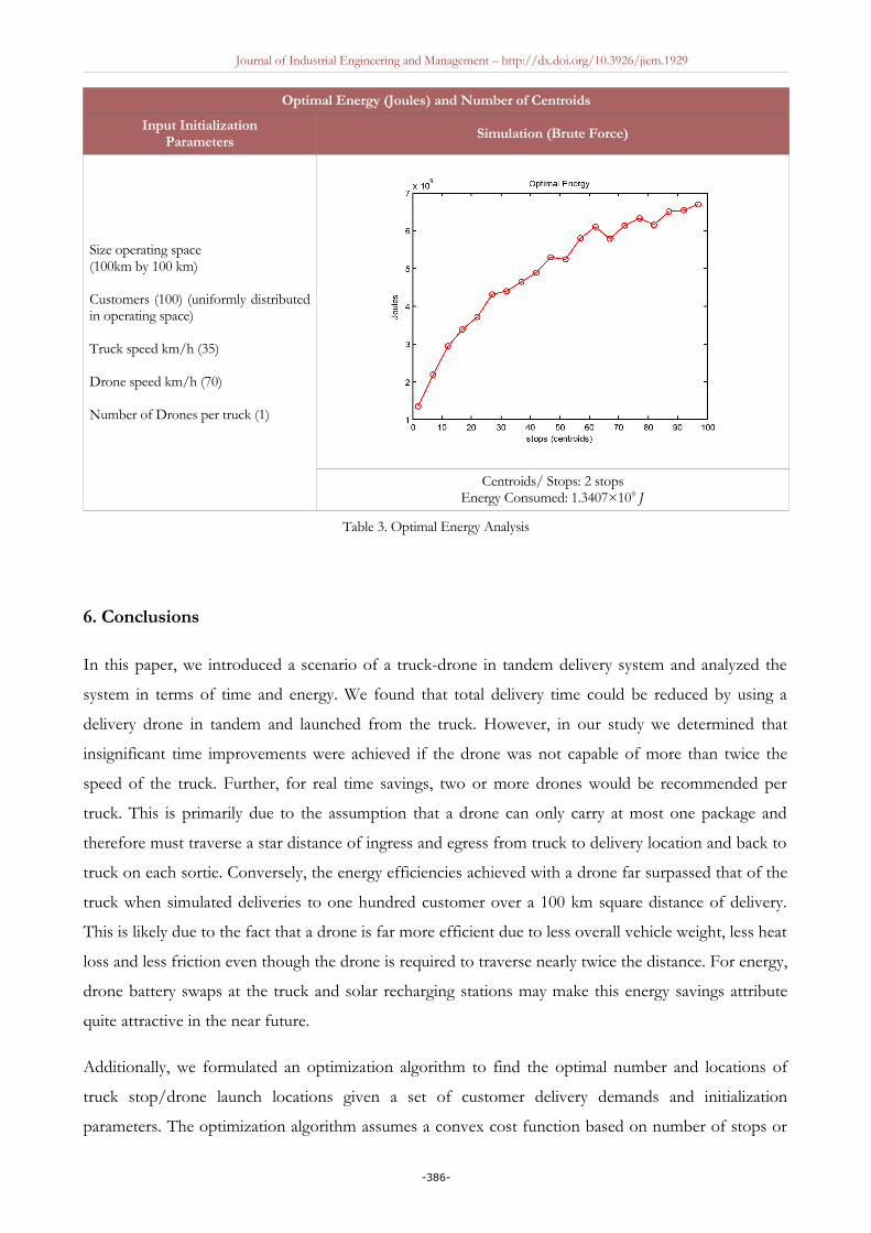
Journal of Industrial Engineering and Management – http://dx.doi.org/10.3926/jiem.1929
Optimal Energy (Joules) and Number of Centroids
Input InitializationParameters
Simulation (Brute Force)
Size operating space (100km by 100 km)
Customers (100) (uniformly distributedin operating space)
Truck speed km/h (35)
Drone speed km/h (70)
Number of Drones per truck (1)
Centroids/ Stops: 2 stopsEnergy Consumed: 1.3407×10⁹ J
Table 3. Optimal Energy Analysis
6. Conclusions
In this paper, we introduced a scenario of a truck-drone in tandem delivery system and analyzed the
system in terms of time and energy. We found that total delivery time could be reduced by using a
delivery drone in tandem and launched from the truck. However, in our study we determined that
insignificant time improvements were achieved if the drone was not capable of more than twice the
speed of the truck. Further, for real time savings, two or more drones would be recommended per
truck. This is primarily due to the assumption that a drone can only carry at most one package and
therefore must traverse a star distance of ingress and egress from truck to delivery location and back to
truck on each sortie. Conversely, the energy efficiencies achieved with a drone far surpassed that of the
truck when simulated deliveries to one hundred customer over a 100 km square distance of delivery.
This is likely due to the fact that a drone is far more efficient due to less overall vehicle weight, less heat
loss and less friction even though the drone is required to traverse nearly twice the distance. For energy,
drone battery swaps at the truck and solar recharging stations may make this energy savings attribute
quite attractive in the near future.
Additionally, we formulated an optimization algorithm to find the optimal number and locations of
truck stop/drone launch locations given a set of customer delivery demands and initialization
parameters. The optimization algorithm assumes a convex cost function based on number of stops or
-386-

Journal of Industrial Engineering and Management – http://dx.doi.org/10.3926/jiem.1929
centroids. Since the problem is simulated and considered quasi-discontinuous, we used difference
equations in place of the Jacobian (gradient) for gradient descent. The algorithm proved to be capable
of solving problems with 200 or more customers in approximately two minutes by solving TSP as well
as drone star-distance. The algorithms found the optimal number and location of truck stops such that
the minimum amount of time was achieved. Several experiments were conducted using the
optimization algorithm and good approximation mathematical models were formulated as closed form
mathematical solutions for expected delivery time and optimal number of stops. Brute force
experiments were conducted to show all relevant outputs regarding a set of likely initialization
parameters. The graphical results show number of stops and the resulting energy and time associated to
each stop given a set of initialization parameters. It was found that efficiencies could always be found in
energy if the drone was not constrained by range. Furthermore, efficiencies in time were found, if the
speed of the drone was approximately three times (or more) as that of the truck, or if two or more
drones were assigned to each truck.
References
Allain, R. (2013). Physics of the Amazon octocopter drone. Wired.
Chen, M., & Macdonald, J. (2014). Optimal Routing Algorithm in Swarm Robotic Systems. Department of Computer
Sciences, California Institute of Technology. Available at:
http://courses.cms.caltech.edu/cs145/2014/ourobouy.pdf
Clarke, G., & Wright, J. (1964). Scheduling of vehicles from a central depot to a number. Operations
research, 12, 568-581. http://dx.doi.org/10.1287/opre.12.4.568
Dantzi, G., & Ramser, J. (1959). The truck dispatching problem. Management Science, 6(1), 80-91.
http://dx.doi.org/10.1287/mnsc.6.1.80
Desrochers, M., Lenstra, J., & Savelsbergh, M. (1990). A classification scheme for vehicle routing and
scheduling problem. Journal of Operations Research Society, 46, 322-332. http://dx.doi.org/10.1016/0377-
2217(90)90007-x
Kirk, J. (2007). Traveling Salesman Problem: Genetic Algorithm. Natick, MA, USA.
MacQueen, J. (1967). Some Methods for classification and Analysis of Multivariate Observations.
Proceedings of 5-th Berkeley Symposium on Mathematical Statistics and Probability. Berkeley: University of
California Press.
-387-

Journal of Industrial Engineering and Management – http://dx.doi.org/10.3926/jiem.1929
MathWorks, I. (2013). KMEANS.
Murray, C., & Chu, A. (2015). The flying sidekick traveling salesman problem: optimization of drone-
assisted parcel delivery. Transportation Research Part C, 54, 86-109. http://dx.doi.org/10.1016/j.trc.2015.03.005
Seber, G. (1984). Multivariate Observations. New York: Wiley. http://dx.doi.org/10.1002/9780470316641
Spath, H. (1985). Cluster Dissection and Analysis: Theory, FORTRAN Programs, Examples. New York:
Halsted Press.
Journal of Industrial Engineering and Management, 2016 (www.jiem.org)
Article's contents are provided on an Attribution-Non Commercial 3.0 Creative commons license. Readers are allowed to copy,
distribute and communicate article's contents, provided the author's and Journal of Industrial Engineering and Management's
names are included. It must not be used for commercial purposes. To see the complete license contents, please visit
http://creativecommons.org/licenses/by-nc/3.0/.
-388-