Embed Size (px)
Citation preview
Optimization Methods for Power Grid Reliability
Sean Harnett
Submitted in partial fulfillment of the
requirements for the degree
of Doctor of Philosophy
in the Graduate School of Arts and Sciences
COLUMBIA UNIVERSITY
2016

c©2016
Sean Harnett
All Rights Reserved
ABSTRACT
Optimization Methods for Power Grid Reliability
Sean Harnett
This dissertation focuses on two specific problems related to the reliability of the modern power
grid. The first part investigates the economic dispatch problem with uncertain power sources. The
classic economic dispatch problem seeks generator power output levels that meet demand most
efficiently; we add risk-awareness to this by explicitly modeling the uncertainty of intermittent
power sources using chance-constrained optimization and incorporating the chance constraints
into the standard optimal power flow framework. The result is a dispatch of power which is
substantially more robust to random fluctuations with only a small increase in economic cost.
Furthermore, it uses an algorithm which is only moderately slower than the conventional practice.
The second part investigates “the power grid attack problem”: aiming to maximize disruption
to the grid, how should an attacker distribute a budget of “damage” across the power lines? We
formulate it as a continuous problem, which bypasses the combinatorial explosion of a discrete
formulation and allows for interesting attacks containing lines that are only partially damaged
rather than completely removed. The result of our solution to the attack problem can provide
helpful information to grid planners seeking to improve the resilience of the power grid to outages
and disturbances. Both parts of this dissertation include extensive experimental results on a
number of cases, including many realistic large-scale instances.
Contents
List of Figures v
List of Tables ix
1 Introduction 1
2 Power grid preliminaries 3
2.1 Structure of power grids . . . . . . . . . . . . . . . . . . . . . . . . . . . . . . 3
2.2 Power grid stability requirements . . . . . . . . . . . . . . . . . . . . . . . . . 4
2.2.1 Frequency stability . . . . . . . . . . . . . . . . . . . . . . . . . . . . . 4
2.2.2 Voltage stability . . . . . . . . . . . . . . . . . . . . . . . . . . . . . . 5
2.2.3 Line stability . . . . . . . . . . . . . . . . . . . . . . . . . . . . . . . . 5
2.3 The power balance equations . . . . . . . . . . . . . . . . . . . . . . . . . . . 6
2.4 The power flow problem . . . . . . . . . . . . . . . . . . . . . . . . . . . . . . 9
2.4.1 Existence and uniqueness of solutions . . . . . . . . . . . . . . . . . . . 10
2.4.2 DC approximation . . . . . . . . . . . . . . . . . . . . . . . . . . . . . 10
2.5 Power flow examples . . . . . . . . . . . . . . . . . . . . . . . . . . . . . . . . 11
2.5.1 Power circles . . . . . . . . . . . . . . . . . . . . . . . . . . . . . . . . 11
2.5.2 Nose curves . . . . . . . . . . . . . . . . . . . . . . . . . . . . . . . . 15
2.5.3 No solution . . . . . . . . . . . . . . . . . . . . . . . . . . . . . . . . . 16
2.5.4 Multiple solutions . . . . . . . . . . . . . . . . . . . . . . . . . . . . . 16
i
2.6 Optimal power flow problem . . . . . . . . . . . . . . . . . . . . . . . . . . . . 18
2.6.1 Difficulties solving the OPF . . . . . . . . . . . . . . . . . . . . . . . . 19
2.6.2 Semidefinite relaxation of the OPF . . . . . . . . . . . . . . . . . . . . 20
2.7 Difficult optimal power flow examples . . . . . . . . . . . . . . . . . . . . . . . 23
2.7.1 Two-bus OPF with local solutions . . . . . . . . . . . . . . . . . . . . . 24
2.7.2 Different solvers converge to different solutions . . . . . . . . . . . . . . 24
2.7.3 Failure to converge after many iterations . . . . . . . . . . . . . . . . . 26
I The economic dispatch problem with uncertain power sources 27
3 Introduction 28
3.1 Transmission system controls . . . . . . . . . . . . . . . . . . . . . . . . . . . 31
3.2 Standard generation dispatch . . . . . . . . . . . . . . . . . . . . . . . . . . . 32
3.3 Adjusting to power fluctuations . . . . . . . . . . . . . . . . . . . . . . . . . . 34
3.4 Using chance constraints . . . . . . . . . . . . . . . . . . . . . . . . . . . . . . 36
3.5 Uncertain power sources . . . . . . . . . . . . . . . . . . . . . . . . . . . . . . 38
3.6 Affine Control . . . . . . . . . . . . . . . . . . . . . . . . . . . . . . . . . . . 39
3.7 Overview of the CC-OPF solution methodology . . . . . . . . . . . . . . . . . . 40
4 Solving the chance-constrained OPF problem 42
4.1 Chance-constrained optimal power flow: formal expression . . . . . . . . . . . . 42
4.1.1 Preliminaries . . . . . . . . . . . . . . . . . . . . . . . . . . . . . . . . 43
4.1.2 Formal expression . . . . . . . . . . . . . . . . . . . . . . . . . . . . . 45
4.1.3 Objective . . . . . . . . . . . . . . . . . . . . . . . . . . . . . . . . . . 46
4.1.4 Variance of the line flow fkm . . . . . . . . . . . . . . . . . . . . . . . 47
4.2 Formulating the chance-constrained problem as a conic program . . . . . . . . . 48
4.3 Solving the conic program . . . . . . . . . . . . . . . . . . . . . . . . . . . . . 51
4.3.1 Example of typical performance of the cutting plane algorithm . . . . . . 54
ii
5 Numerical experiments 56
5.1 Failure of standard OPF . . . . . . . . . . . . . . . . . . . . . . . . . . . . . . 57
5.2 Cost of reliability under high wind penetration . . . . . . . . . . . . . . . . . . 58
5.3 Non-locality . . . . . . . . . . . . . . . . . . . . . . . . . . . . . . . . . . . . 60
5.4 Increasing penetration . . . . . . . . . . . . . . . . . . . . . . . . . . . . . . . 61
5.5 Out-of-sample tests . . . . . . . . . . . . . . . . . . . . . . . . . . . . . . . . 61
5.6 Scalability . . . . . . . . . . . . . . . . . . . . . . . . . . . . . . . . . . . . . 65
5.7 Changing locations for wind farms . . . . . . . . . . . . . . . . . . . . . . . . . 66
5.8 Reversal of line flows . . . . . . . . . . . . . . . . . . . . . . . . . . . . . . . . 66
II The power grid attack problem 68
6 Introduction 69
6.1 Motivation . . . . . . . . . . . . . . . . . . . . . . . . . . . . . . . . . . . . . 69
6.1.1 Continuous formulation . . . . . . . . . . . . . . . . . . . . . . . . . . 70
6.1.2 Is this realistic? . . . . . . . . . . . . . . . . . . . . . . . . . . . . . . 71
6.2 Attacker budget and the upper-level problem . . . . . . . . . . . . . . . . . . . 72
6.3 Optimal power flow lower-level problem . . . . . . . . . . . . . . . . . . . . . . 73
6.4 Related work . . . . . . . . . . . . . . . . . . . . . . . . . . . . . . . . . . . . 76
7 Solving the attack problem 78
7.1 Solving the OPF lower-level problem . . . . . . . . . . . . . . . . . . . . . . . 79
7.2 Non-convexity and multiple local optima . . . . . . . . . . . . . . . . . . . . . 79
7.3 The Frank-Wolfe algorithm . . . . . . . . . . . . . . . . . . . . . . . . . . . . 80
7.3.1 Example . . . . . . . . . . . . . . . . . . . . . . . . . . . . . . . . . . 83
7.4 Computing the gradient . . . . . . . . . . . . . . . . . . . . . . . . . . . . . . 83
7.5 Other approaches . . . . . . . . . . . . . . . . . . . . . . . . . . . . . . . . . 84
7.5.1 Derivative-free optimization . . . . . . . . . . . . . . . . . . . . . . . . 84
iii
7.5.2 Branching . . . . . . . . . . . . . . . . . . . . . . . . . . . . . . . . . 85
8 Numerical experiments 87
8.1 9-bus example . . . . . . . . . . . . . . . . . . . . . . . . . . . . . . . . . . . 87
8.1.1 Attack parameters . . . . . . . . . . . . . . . . . . . . . . . . . . . . . 88
8.1.2 Results . . . . . . . . . . . . . . . . . . . . . . . . . . . . . . . . . . . 88
8.1.3 Summary . . . . . . . . . . . . . . . . . . . . . . . . . . . . . . . . . . 89
8.2 57-bus example: branching . . . . . . . . . . . . . . . . . . . . . . . . . . . . 90
8.3 118-bus example: head and tail . . . . . . . . . . . . . . . . . . . . . . . . . . 94
8.4 Large-scale example on the Polish grid . . . . . . . . . . . . . . . . . . . . . . 95
Bibliography 98
iv
List of Figures
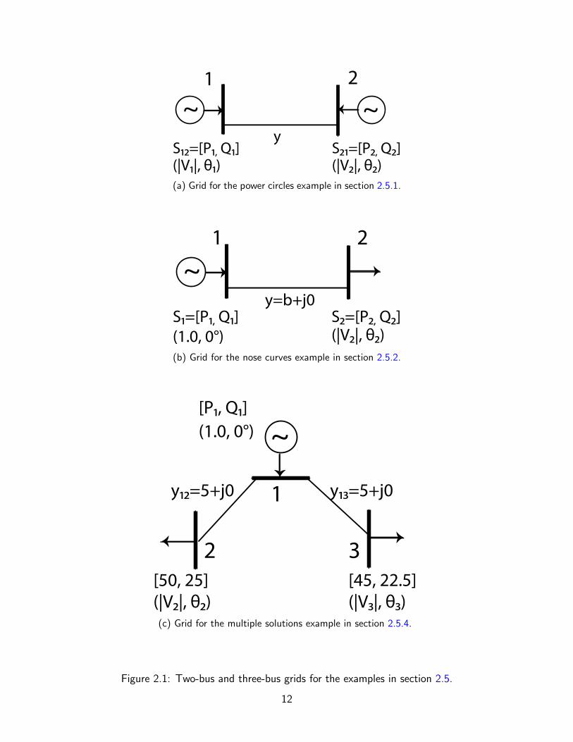
2.1 Two-bus and three-bus grids for the examples in section 2.5. . . . . . . . . . . . 12
2.2 Sending-end and receiving-end circles from [17]. Both circles have radius |B| =
|y||V1||V2|. . . . . . . . . . . . . . . . . . . . . . . . . . . . . . . . . . . . . . 14
2.3 Nose curves for two bus example from [29] with b = −10. Notice how as P2
increases from zero there are first two solutions, then one solution, and finally no
solutions for each load factor. . . . . . . . . . . . . . . . . . . . . . . . . . . . 16
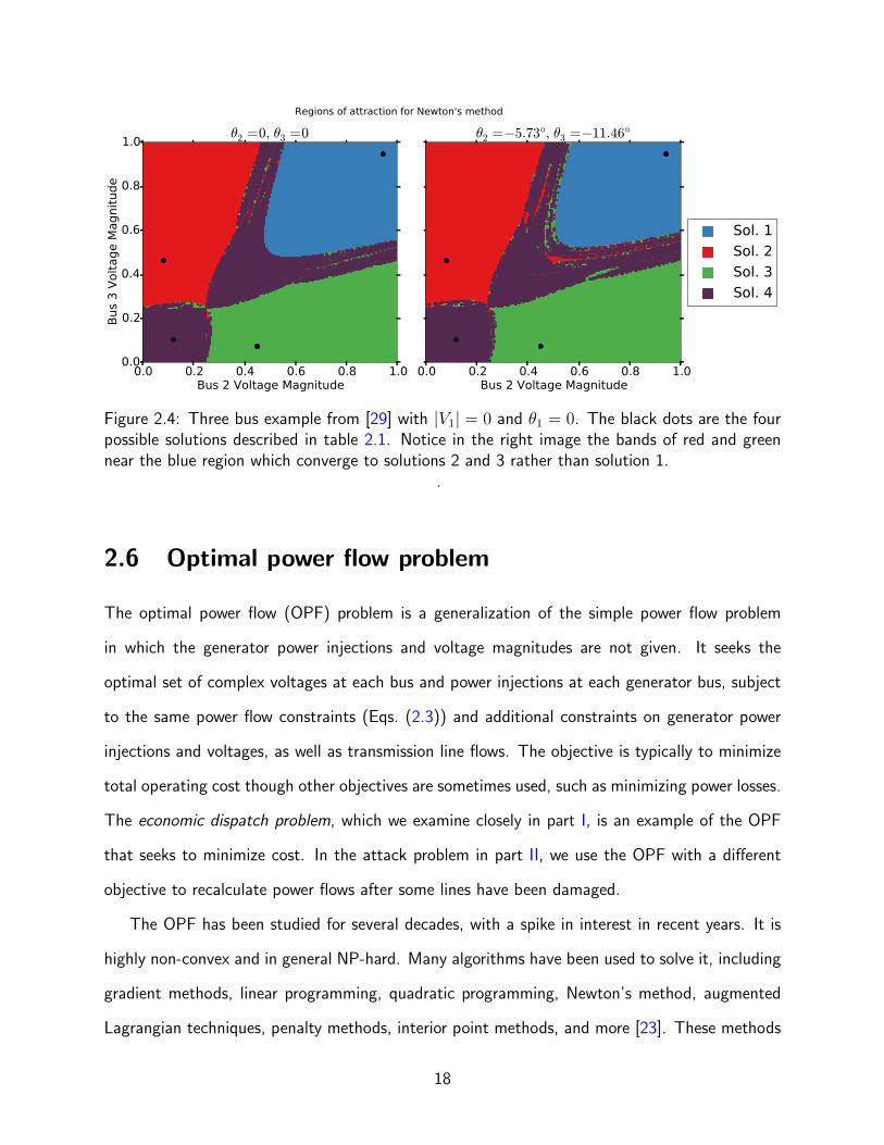
2.4 Three bus example from [29] with |V1| = 0 and θ1 = 0. The black dots are the
four possible solutions described in table 2.1. Notice in the right image the bands
of red and green near the blue region which converge to solutions 2 and 3 rather
than solution 1. . . . . . . . . . . . . . . . . . . . . . . . . . . . . . . . . . . 18
2.5 Two bus grid from [22]. Note that we use the impedance z rather than the
admittance y in this example. . . . . . . . . . . . . . . . . . . . . . . . . . . . 24
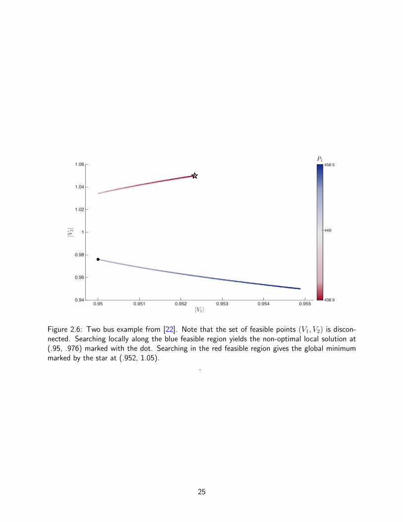
2.6 Two bus example from [22]. Note that the set of feasible points (V1, V2) is
disconnected. Searching locally along the blue feasible region yields the non-
optimal local solution at (.95, .976) marked with the dot. Searching in the red
feasible region gives the global minimum marked by the star at (.952, 1.05). . . 25
v
3.1 Bonneville Power Administration [8] shown in outline under 9% wind penetration,
where green dots mark actual wind farms. We set standard deviation to be 0.3
of the mean for each wind source. Our CC-OPF (with 1% of overload set as
allowable) resolved the case successfully (no overloads) and was computed in
seconds, while the standard OPF showed 8 overloaded lines, all marked in color.
Lines shown orange are at 4% chance of overload. There are two dark red lines
which are at 50% of the overload while other (dark orange) lines show values of
overload around 10%. . . . . . . . . . . . . . . . . . . . . . . . . . . . . . . . 29
5.1 118-bus case with four wind farms (green dots; brown are generators, black are
loads). Shown is the standard OPF solution against the average wind case with
penetration of 5%. Standard deviations of the wind are set to 30% of the respec-
tive average cases. Lines in red exceed their limit 8% or more of the time. . . . 58
5.2 39-bus case. Red lines indicate high probability of flow exceeding the limit under
the standard OPF solution. Generators are shades of blue, with darker shades
indicating greater absolute difference between the chance-constrained solution
and the standard solution. . . . . . . . . . . . . . . . . . . . . . . . . . . . . . 60
5.3 39-bus case with four wind farms (green dots; brown are generators, black are
loads). Lines in red are at the maximum of ε = .02 chance of exceeding their
limit. The three cases shown are left to right: .1%, 8%, and 30% average wind
penetration. With penetration beyond 30% the problem becomes infeasible. . . . 62
5.4 30-bus case with three wind farms. The case on the left supports only up to
10% before becoming infeasible, while the one on the right is feasible up to 55%
penetration. . . . . . . . . . . . . . . . . . . . . . . . . . . . . . . . . . . . . 62
5.5 Maximum probability of overload for out-of-sample tests. These are a result of
Monte Carlo testing with 10,000 samples on the BPA case, solved under assuming
normally distributed fluctuations and desired maximum chance of overload at
2.27%. . . . . . . . . . . . . . . . . . . . . . . . . . . . . . . . . . . . . . . 64
vi
5.6 BPA case solved with average penetration at 8% and standard deviations set to
30% of mean. The maximum probability of line overload desired is 2.27%, which
is achieved with 0 forecast error on the graph. Actual wind power means are
then scaled according to the x-axis and maximum probability of line overload is
recalculated (blue). The same is then done for standard deviations (green). . . 64
5.7 Number of lines that are overloaded with given probability values in simulation
of 2746 bus Polish power grid with 20% wind penetration distributed over 50
wind farms. Under the standard OPF, five lines are overloaded half of the time,
and two lines are overloaded more than ten percent of the time, constituting a
situation with unacceptable systemic risk. Under the chance-constrained OPF,
the largest overload probability is fifty times smaller than in the case of standard
OPF. Moreover, the cost increase is by less than five percent. . . . . . . . . . . 65
5.8 9-bus case, 25% average penetration from two wind sources. With shifting winds,
the flow on the orange line changes direction with a large absolute difference. . . 67
7.1 The attack problem is non-convex and can have multiple local optima. The left
image shows all attacks on lines 2, 3 and 3, 4 from case5 up to a maximum
of γ = 2.5. The global optimum is (2.5, 2.5) but there is a local optimum at (.66,
0). Restricting to the x-axis or the dotted line γ34 = 2.5− γ23 results in the right
image, with different local and global optima; see the text for details. Random
restarts of the Frank-Wolfe procedure help to find a good local optimum. . . . 80
7.2 Two different line search approaches for the Frank-Wolfe algorithm applied to
minimizing f(x, y) = (x− 2)2 + 5(y − 2)2 in the region x ≥ 0, y ≥= 0, x+ y ≤
3. An exact line search suffers from zig-zagging and takes many iterations to
converge; a simple back-tracking line search quickly finds the optimum. . . . . . 84
8.1 case9 from MATPOWER, rendered by graphviz [34]. Generator buses are in green,
load buses are in black. Buses with neither demand nor generation are grey. . . . 88
vii

8.2 Three different attacks on case9, where a red dotted line has its impedance multi-
plied by 3.5. F is the attacker’s objective, in this case maximizing the 1-norm of
phase angle differences across branches (the units are degrees). H is the objective
for the OPF inner problem. The unattacked grid has F = 33.249 and H = 0. . . 90
8.3 As the attack grows stronger, many different indicators of grid health grow weaker.
“Null” is the unattacked grid; see the text for definitions of weak, median, and
strong attacks. Branch apparent power is defined here as S = 12
(√P 2f +Q2
f +√P 2t +Q2
t
)– the average of the apparent power injected into the line from the ‘to’ bus and
the ‘from’ bus. . . . . . . . . . . . . . . . . . . . . . . . . . . . . . . . . . . . 91
8.4 case57 from MATPOWER with generator buses in green. Pictured are two attacks
discovered with the branching procedure in section 8.2. Observe that the attacks
are qualitatively different: the attack on the left creates two islands, while the
attack on the left focuses on generators and heavily loaded lines. . . . . . . . . 92
8.5 The branching procedure applied to case57. The first of each pair of lines in-
cates which branches are excluded from the attack. The second is of the form:
objective [branch number attack value; branch number attack value;
...]. Forcing certain lines to be excluded from the attack may find other sets of
vulnerable lines, and sometimes improves the strength of the attack. . . . . . . . 93
8.6 Histogram of phase angle differences under different attacks on case118. Notice
that the Frank-Wolfe attack increases the phase angle difference on many branches
to over 20 degrees. . . . . . . . . . . . . . . . . . . . . . . . . . . . . . . . . 95
8.7 The IEEE 118-bus test system. (Image source: [1].) . . . . . . . . . . . . . . . 96
8.8 Sample output from the Frank-Wolfe attack procedure on case118 from a zero
start. . . . . . . . . . . . . . . . . . . . . . . . . . . . . . . . . . . . . . . . . 96
8.9 Output from the Frank-Wolfe attack procedure on case2383wp from a zero start.
Included are the step-size used in the line-search step as well as run times (in
seconds) for the line search and gradient steps. . . . . . . . . . . . . . . . . . . 97
viii
List of Tables
2.1 Solutions to the three-bus system. . . . . . . . . . . . . . . . . . . . . . . . . . 17
4.1 Performance of cutting-plane method on a number of large cases. . . . . . . . 54
4.2 Typical convergence behavior of cutting-plane algorithm on a large instance. . . 55
5.1 Impact of penetration, 39-bus case . . . . . . . . . . . . . . . . . . . . . . . . 59
7.1 A typical example comparing the effectiveness of a derivative-free optimization
method to our gradient-based method on the attack problem. The Frank-Wolfe
method finds better attacks and requires far fewer function evaluations. Runtimes
were computed from a single core of an Intel Xeon X5570 2.93GHz machine. . . 85
8.1 Attack problem parameters for case9 example . . . . . . . . . . . . . . . . . . . 88
8.2 Changes in power generation after the strong attack. Pg is real power output,
Qg is reactive. In the strong attack, lines 1,4, 5,6, and 8,9 have their
impedance multiplied by 3.5. . . . . . . . . . . . . . . . . . . . . . . . . . . . 89
8.3 Objective values for different attacks on case118. See the text for the definitions
of the different attacks. . . . . . . . . . . . . . . . . . . . . . . . . . . . . . . 94
ix
Chapter 1
Introduction
The development of the power grid and the electricity it provides has led to tremendous economic
and social progress, dramatically improving quality of life across the globe. It underlies virtually
every aspect of our modern economy and society.
The energy landscape, however, is changing dramatically. One significant change is that much
more of our energy is coming from renewable sources. Spurred by improvements in technology
and concerns with climate change, the U.S. has increased its solar electricity generation by 20-
fold since 2008, and more than tripled electricity generation from wind energy [9]. This trend
is expected to continue across the world’s power grids. For example Germany, a world leader in
renewable energy, expects to grow its renewable penetration from 30% in 2014 to 80% in 2050.
Such high renewable penetration creates challenges for power grids like those in the U.S. which
were built under the assumption of almost entirely dispatchable generation. The intermittent
nature of many renewable energy sources requires the power grid to adapt from this old design
to maximally take advantage of these energy sources in a safe and efficient manner.
Innovations in smart grid technology, of which increasing renewable energy plays a large
part, are leading to an ever more complex power grid. At the same time, demand for power
continues to increase at a faster pace than supporting infrastructure, so that the grid operates
closer to capacity with smaller safety margins [42]. As a consequence, power outages and quality
1

disturbances are becoming more frequent, costing the U.S. economy an estimated $80 to $188
billion a year [12]. Recent large-scale blackouts [2] [5] provide a clear reminder of this problem.
The growing complexity of the grid suggests that without new ideas and measures, these blackouts
will become more frequent and more costly.
This dissertation focuses on two specific problems related to the reliability of the modern
power grid. In part I we investigate the economic dispatch problem with uncertain power sources.
In this, we add risk awareness to the classic problem of determining how much power generators
should produce to meet demand most efficiently. We do this by explicitly modeling the uncertainty
of intermittent power sources and directly addressing the risk of line flow overages when power
outputs vary significantly from their forecasted values.
In part II we investigate the “the power grid attack problem”: aiming to maximize damage
to the grid, how would an attacker distribute a budget of “damage” across the power lines? It
is a continuous and therefore more tractable version of the “N-k” problem, which seeks to find
a set of k lines in a grid with N lines whose removal will maximally disrupt the grid. By helping
to identify vulnerable components in the power grid, the study of this problem can provide useful
information to grid planners seeking to improve the resilience of the power grid to outages and
disturbances.
2

Chapter 2
Power grid preliminaries
This chapter introduces the background material on power systems needed to understand the
chapters that follow. The chapter describes basic power grid concepts, the power balance equa-
tions, and the load flow and optimal power flow problems that use them. It also includes some
examples of simple power flow situations to help provide intuition as to how power flows behave.
2.1 Structure of power grids
The power grid can be thought of as a graph, with power lines as edges and generators and loads
as vertices. The graph has two systems: 1) a high voltage (hundreds of kV) transmission system
connecting power plants to electrical substations and 2) a medium voltage (tens of kV) distribution
system connecting the substations to individual consumers, at which point the voltage is lowered
to 120V in the U.S. The voltage levels of the different systems take advantage of different points
in the trade-off between the efficiency of high voltage transmission and the safety of low voltage
distribution (which occurs closer to buildings and people).
The graph of the medium voltage distribution system typically has a tree structure which
can be exploited for certain problems. The problems considered in this thesis focus on the
transmission system, however, which almost always includes cycles. Both systems use primarily
alternating current (AC) power lines, though direct current (DC) is occasionally used in particular
3

situations in the transmission system.
Some terminology: the term bus is used to describe a vertex in the graph, usually either a
generator, a load, or a transformer. The term branch refers to an edge in the graph – a power
line.
As a matter of convenience, a rescaling of variables known as the per unit (or p.u.) system
is almost always used in power systems analysis [17]. For example, power quantities may be
scaled by 100MVA and voltages by 135KV. This is especially convenient when there are many
transformers, since the per-unit quantities do not change on either side of a transformer. The
system is also useful when there are many voltage levels involved; because voltage magnitudes
will be close to their nominal values under stable conditions (see the next section), they are all
close to 1.0 p.u. in the per-unit system, and it is easy to quickly identify buses with undesirable
voltage levels.
2.2 Power grid stability requirements
2.2.1 Frequency stability
The power grid operates at a fixed frequency, 60 Hz in the U.S., with all generators producing
power in sync. If two generators lose synchronism or “fall out of step,” they no longer generate
voltages of the same frequency, and effective exchange of power ceases. Furthermore, because
generators are specifically designed and calibrated to operate within a narrow band (≈ ±0.05Hz)
of the prescribed frequency, large deviations in frequency can be very damaging to the equipment.
For these reasons, automatic control systems (see section 3.1 for more) act very quickly to
synchronize the grid to the desired frequency. In some cases, it may be necessary to trip a
generator (detach it from the grid) in order to protect it from unsafe frequency deviations, which
can lead to further frequency deviations and a dangerous vicious cycle.
4
2.2.2 Voltage stability
Similarly, the grid operates most efficiently when all buses are kept at voltage magnitudes of
1.0 p.u. When grid conditions force voltages to stray too far from 1.0, a number of problems
arise. This type of disturbance usually appears as a voltage drop and when voltages become low
enough the system cannot maintain stability. This situation is known as voltage collapse. It is
a well-studied phenomenon [30] involved in numerous historical blackouts, in particular the 2003
Northeast blackout [2].
2.2.3 Line stability
Power lines can fail when they carry too much power, most commonly in the case of thermal
overload. Excessive power over a line will cause it to overheat and the conducting material to
degrade. But before that occurs, the line will sag and become much more likely to touch or
create an arc with a foreign object, leading to a short circuit. It takes some time for power lines
to heat up, and this usually does not become dangerous for minutes or hours, leaving enough
time for grid operators to shed load or redispatch power. In general, it is not a great risk when
the flow on a line exceeds the limit for a short period of time. To help address the problem of
thermal overload, power lines come with a standard rating and one or more emergency ratings
which determine the amount of power that can be safely transmitted. Each level of rating has a
maximum amount of time that the line can carry that much power before grid operators need to
relieve it.
A more pressing risk to grid stability from power lines is high phase angle difference. When the
phase angle difference between two buses becomes too high, the two buses will lose synchronism,
leading to the problems discussed above for frequency stability. The upper limit to the phase
angle difference depends on a number of factors, but it is typically more restrictive for longer
lines [17].
For example, in the 2011 San Diego blackout, a long line was accidentally opened. The grid
then adjusted and entered a dangerous state, while simultaneously the phase angle difference
5

across the line grew very large. The angle was too large for operators to reclose the line without
losing synchrony and an immediate failure of the grid, so it remained open. The dangerous state
of the grid persisted and led to a cascading blackout [5] which left millions in the greater San
Diego area without electricity in what would become the largest power failure in California history.
2.3 The power balance equations
The flow of electric power on a network is governed by the laws of physics, and under stable
conditions can be accurately described by the steady-state1 power balance equations derived in
this section. For other descriptions of this material, see [17] and [13]. First, some notation:
• j =√−1 is the imaginary unit
• E is the set of all lines (edges) in the grid
• V is the set of all buses (vertices) in the grid
• G is the set of generator buses
• D is the set of load (demand) buses
• k and m are bus indices
• K is the set of buses adjacent to bus k, including bus k
• Ωk is the set of buses adjacent to bus k, excluding bus k
• km refers to the power line from bus k to bus m
• k,m also refers to the power line between buses k and m, but as an unordered pair
• θkm = θk − θm is the phase angle difference between buses k and m
1The problems addressed in this thesis do not consider transients and other behaviors which can be describedby differential equations.
6
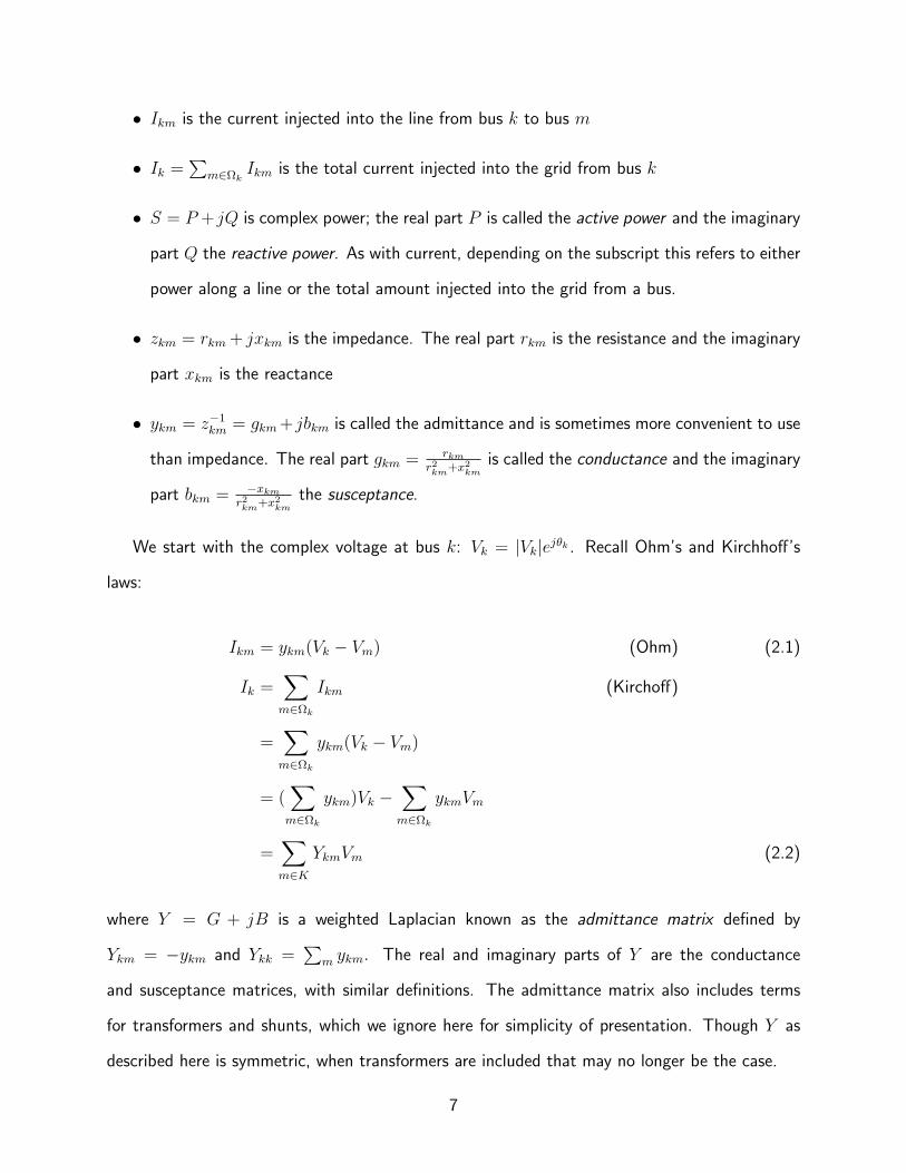
• Ikm is the current injected into the line from bus k to bus m
• Ik =∑
m∈ΩkIkm is the total current injected into the grid from bus k
• S = P + jQ is complex power; the real part P is called the active power and the imaginary
part Q the reactive power. As with current, depending on the subscript this refers to either
power along a line or the total amount injected into the grid from a bus.
• zkm = rkm + jxkm is the impedance. The real part rkm is the resistance and the imaginary
part xkm is the reactance
• ykm = z−1km = gkm+jbkm is called the admittance and is sometimes more convenient to use
than impedance. The real part gkm = rkmr2km+x2km
is called the conductance and the imaginary
part bkm = −xkmr2km+x2km
the susceptance.
We start with the complex voltage at bus k: Vk = |Vk|ejθk . Recall Ohm’s and Kirchhoff’s
laws:
Ikm = ykm(Vk − Vm) (Ohm) (2.1)
Ik =∑m∈Ωk
Ikm (Kirchoff)
=∑m∈Ωk
ykm(Vk − Vm)
= (∑m∈Ωk
ykm)Vk −∑m∈Ωk
ykmVm
=∑m∈K
YkmVm (2.2)
where Y = G + jB is a weighted Laplacian known as the admittance matrix defined by
Ykm = −ykm and Ykk =∑
m ykm. The real and imaginary parts of Y are the conductance
and susceptance matrices, with similar definitions. The admittance matrix also includes terms
for transformers and shunts, which we ignore here for simplicity of presentation. Though Y as
described here is symmetric, when transformers are included that may no longer be the case.
7
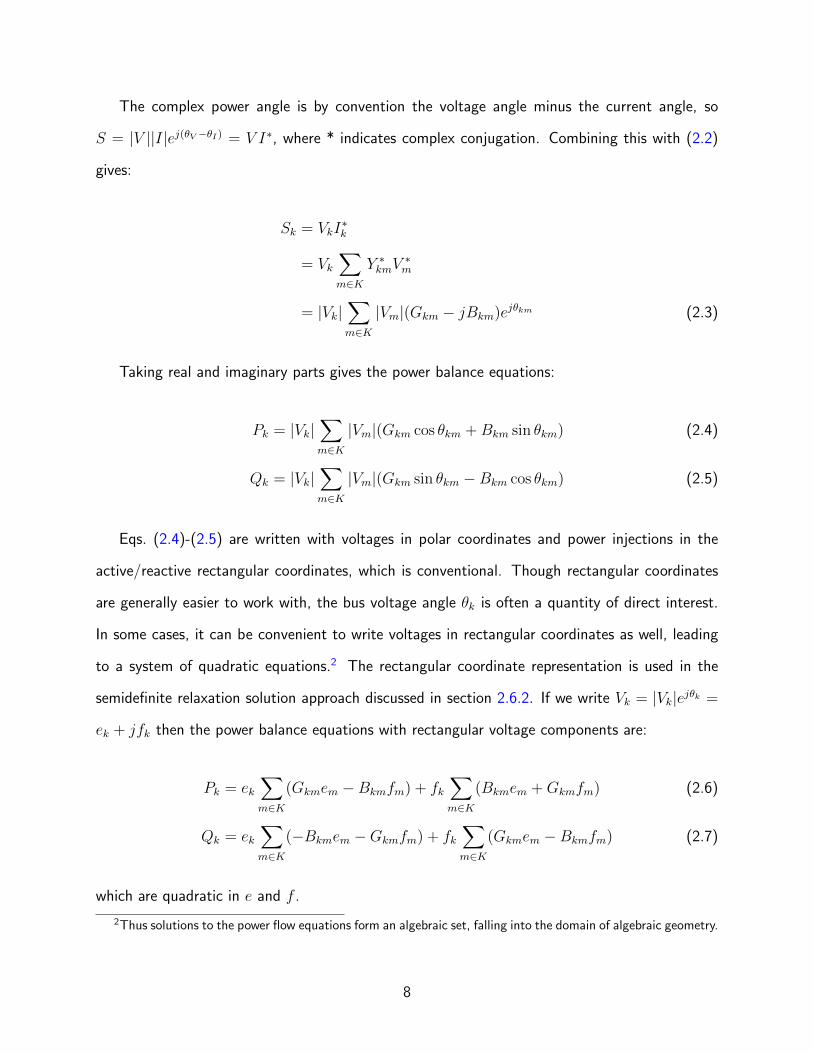
The complex power angle is by convention the voltage angle minus the current angle, so
S = |V ||I|ej(θV −θI) = V I∗, where * indicates complex conjugation. Combining this with (2.2)
gives:
Sk = VkI∗k
= Vk∑m∈K
Y ∗kmV∗m
= |Vk|∑m∈K
|Vm|(Gkm − jBkm)ejθkm (2.3)
Taking real and imaginary parts gives the power balance equations:
Pk = |Vk|∑m∈K
|Vm|(Gkm cos θkm +Bkm sin θkm) (2.4)
Qk = |Vk|∑m∈K
|Vm|(Gkm sin θkm −Bkm cos θkm) (2.5)
Eqs. (2.4)-(2.5) are written with voltages in polar coordinates and power injections in the
active/reactive rectangular coordinates, which is conventional. Though rectangular coordinates
are generally easier to work with, the bus voltage angle θk is often a quantity of direct interest.
In some cases, it can be convenient to write voltages in rectangular coordinates as well, leading
to a system of quadratic equations.2 The rectangular coordinate representation is used in the
semidefinite relaxation solution approach discussed in section 2.6.2. If we write Vk = |Vk|ejθk =
ek + jfk then the power balance equations with rectangular voltage components are:
Pk = ek∑m∈K
(Gkmem −Bkmfm) + fk∑m∈K
(Bkmem +Gkmfm) (2.6)
Qk = ek∑m∈K
(−Bkmem −Gkmfm) + fk∑m∈K
(Gkmem −Bkmfm) (2.7)
which are quadratic in e and f .
2Thus solutions to the power flow equations form an algebraic set, falling into the domain of algebraic geometry.
8

2.4 The power flow problem
Finding a solution to the power balance equations (2.4) and (2.5) for all buses amounts to solving
for the voltage magnitude and angle for each bus, using whichever of the quantities |Vk|, θk, Pk, Qk
that are known as well as static grid data encoded in the Y matrix. Once we know the complex
voltage at each bus, the active and reactive power injections can be immediately computed from
the equations. We generally split the set of buses V into two sets: 1) the set G of generators,
where voltage magnitude and sometimes active power injections are known and 2) the set D (for
demand) of loads, where active and reactive power demands are known.
For a grid with n buses of which m are loads, we have n unknown phase angles and m
unknown voltage magnitudes for a total of n + m unknowns. Since active power injections are
known at each bus, we have n equations of the type (2.4), and since reactive power injections
are known at each load, m equations of type (2.5) for a total of n+m equations.
Conservation of power prevents us from specifying Pk at every bus, however – the sum of all
power injections must equal the sum of power losses on the lines, and the line losses are unknown
in advance. So we leave Pk free at one bus, called the slack bus, to pick up the “slack” and ensure
that the sum of all power injections is equal to the sum of losses. This adds an unknown variable
which would make our system of equations underdetermined. But note that in the equations,
phase angles only appear as differences, so we can arbitrarily assign the phase at one bus (usually
θk = 0) called the reference bus, thus removing one unknown. For convenience we usually let
the slack and reference bus be the same at k = 1. So we indeed have n + m equations and
unknowns, and the hope for a unique solution; see the next section for additional discussion.
The power balance equations are typically solved via Newton’s method. In practice, the
equations are often solved after a small change has occurred in the state of the grid, and the
solution from the previous state is used as the initial guess, in other words a “warm start.” If a
previous solution isn’t available, a “flat start” with |Vk| = 1, θk = 0 ∀k will often converge. If the
grid has changed significantly from the previous known state, however, Newton’s method may
fail to converge, even with a warm start. Though there has been much research and progress on
9
solving power flows, this problem continues to be a source of frustration in the study of power
grids. Section 2.6 on the optimal power flow problem, a generalization of the simple power flow
problem, further discusses this issue.
2.4.1 Existence and uniqueness of solutions
In general the system will not have a unique solution; we will see examples in section 2.5 of
systems with zero or multiple solutions. But under normal practical conditions there is usually
exactly one realistic solution: the solution where the voltage magnitudes are all close to 1.0 p.u.
This is because under normal conditions, voltage magnitudes vary slowly and continuously, and
grid operators are actively working to keep them near 1.0.
In general, the number of possible solutions in a grid is exponential in the number of buses [43],
though the actual number of solutions is typically much smaller. The state of the art does not
yet have a tractable way of reliably finding all solutions. The Newton’s method grid-search
method illustrated in the example in section 2.5.4 is impractical for large grids. Homotopy-based
methods [59] may find all solutions, but they have complexity that grows exponentially with the
size of the grid even when the number of actual solutions is small. The semidefinite relaxation
approach discussed in section 2.6 is more efficient, but the relaxation is not tight in general and
thus it is possible for it to find “solutions” which are not physically meaningful.
2.4.2 DC approximation
Though Eqs.(2.4)-(2.5) can be difficult to solve in general, under normal operating conditions they
can be approximated by much simpler linear equations. The DC approximation takes advantage
of the following approximations:
1. Resistance is dominated by reactance: rkm ≈ 0 and thus gkm ≈ 0 for all lines k,m
2. Voltage magnitudes are fixed and scaled to unity: |Vk| ≈ 1 ∀k ∈ V
3. Voltage angle differences are small, so that: sin θkm ≈ θkm for all lines k,m
10

Under these assumptions, the real power balance equation (2.4) simplifies to
Pk = |Vk|∑m
|Vm|(Gkm cos θkm +Bkm sin θkm)
≈∑m
Bkmθkm
We write the DC approximation to the power balance equations as
Bθ = P (2.8)
which relates the real power at each bus to the susceptance matrix and the vector of phase angle
differences across each line. The name DC approximation becomes more clear when we look at
the contribution of a single line to (2.8):
Pkm = Bkmθkm
= −bkm(θk − θm)
=θk − θmxkm
The equation is analagous to Ohm’s law applied to a resistor carrying a DC current, where in the
analogy P represents the current, θ the voltage at each terminal, and x the resistance.
2.5 Power flow examples
2.5.1 Power circles
Here we introduce the concept of power circles, as described in [17]. This should provide some
intuition on the behavior of power flow on a very simple grid. Consider the case of two buses
connected by a single line (figure 2.1). The complex power injected into the grid by bus 1 toward
11
~ ~
yS12=[P1, Q1](|V1|, θ1)
S21=[P2, Q2](|V2|, θ2)
1 2
(a) Grid for the power circles example in section 2.5.1.
~y=b+j0
(1.0, 0°)S1=[P1, Q1] S2=[P2, Q2]
(|V2|, θ2)
1 2
(b) Grid for the nose curves example in section 2.5.2.
y12=5+j0
(1.0, 0°)
(|V3|, θ3)
~
(|V2|, θ2)[50, 25]
y13=5+j0
[45, 22.5]
[P1, Q1]
1
2 3
(c) Grid for the multiple solutions example in section 2.5.4.
Figure 2.1: Two-bus and three-bus grids for the examples in section 2.5.
12
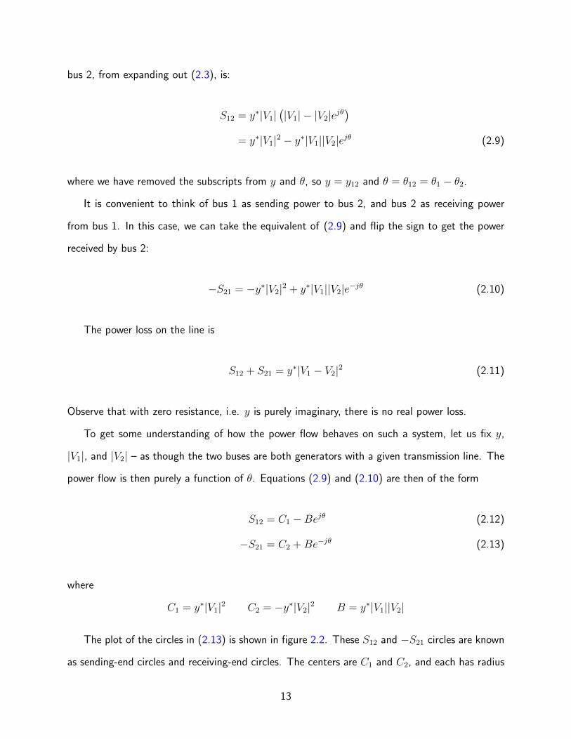
bus 2, from expanding out (2.3), is:
S12 = y∗|V1|(|V1| − |V2|ejθ
)= y∗|V1|2 − y∗|V1||V2|ejθ (2.9)
where we have removed the subscripts from y and θ, so y = y12 and θ = θ12 = θ1 − θ2.
It is convenient to think of bus 1 as sending power to bus 2, and bus 2 as receiving power
from bus 1. In this case, we can take the equivalent of (2.9) and flip the sign to get the power
received by bus 2:
−S21 = −y∗|V2|2 + y∗|V1||V2|e−jθ (2.10)
The power loss on the line is
S12 + S21 = y∗|V1 − V2|2 (2.11)
Observe that with zero resistance, i.e. y is purely imaginary, there is no real power loss.
To get some understanding of how the power flow behaves on such a system, let us fix y,
|V1|, and |V2| – as though the two buses are both generators with a given transmission line. The
power flow is then purely a function of θ. Equations (2.9) and (2.10) are then of the form
S12 = C1 −Bejθ (2.12)
−S21 = C2 +Be−jθ (2.13)
where
C1 = y∗|V1|2 C2 = −y∗|V2|2 B = y∗|V1||V2|
The plot of the circles in (2.13) is shown in figure 2.2. These S12 and −S21 circles are known
as sending-end circles and receiving-end circles. The centers are C1 and C2, and each has radius
13
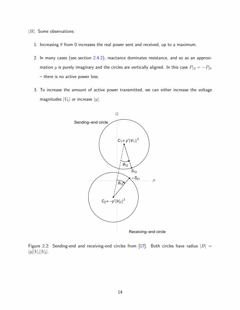
|B|. Some observations:
1. Increasing θ from 0 increases the real power sent and received, up to a maximum.
2. In many cases (see section 2.4.2), reactance dominates resistance, and so as an approxi-
mation y is purely imaginary and the circles are vertically aligned. In this case P12 = −P21
– there is no active power loss.
3. To increase the amount of active power transmitted, we can either increase the voltage
magnitudes |Vk| or increase |y|.
C1= y* |V1
2
C2= -y* |V22
θ12
θ12
S12
-S21
Sending-end circle
Receiving-end circle
P
Q
Figure 2.2: Sending-end and receiving-end circles from [17]. Both circles have radius |B| =|y||V1||V2|.
14
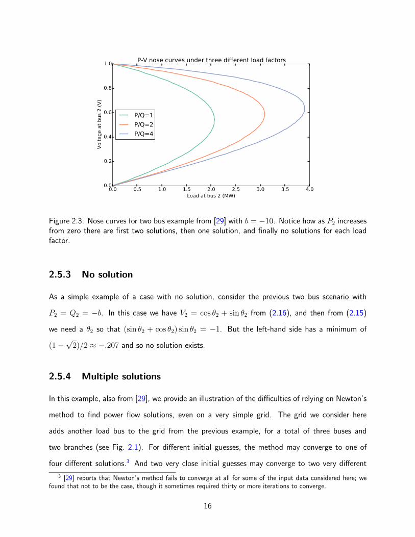
2.5.2 Nose curves
Here we introduce the concept of nose curves as described in [29]. For more on this topic in the
context of voltage stability analysis, see [2, p. 35]. To start, consider a grid with two buses and
a single branch (figure 2.1) with no resistance (and hence no real power loss, i.e. g = 0). Let
bus 1 be a generator with |V1| = 1, θ1 = 0 and let bus 2 be a load. The power flow equations at
bus 2 are:
P2 = bV2 sin θ2 (2.14)
Q2 = b(V 22 − V2 cos θ2) (2.15)
Solving for V2 in terms of θ2 gives
V2 = cos θ2 +1
αsin θ2 (2.16)
where α = P2/Q2 is the load factor. If we consider different load factors, we get different
contours of solutions in the P2 − V2 plane known as nose curves. See figure 2.3, where we have
set the susceptance to b = −10. Notice that depending on the value of P2 there are either 0, 1,
or 2 solutions, and in particular that for a fixed load factor, there is a maximum amount of real
power that can be delivered to the load bus beyond which the flow is infeasible.
15
0.0 0.5 1.0 1.5 2.0 2.5 3.0 3.5 4.0Load at bus 2 (MW)
0.0
0.2
0.4
0.6
0.8
1.0
Volt
age a
t bus
2 (
V)
P-V nose curves under three different load factors
P/Q=1
P/Q=2
P/Q=4
Figure 2.3: Nose curves for two bus example from [29] with b = −10. Notice how as P2 increasesfrom zero there are first two solutions, then one solution, and finally no solutions for each loadfactor.
2.5.3 No solution
As a simple example of a case with no solution, consider the previous two bus scenario with
P2 = Q2 = −b. In this case we have V2 = cos θ2 + sin θ2 from (2.16), and then from (2.15)
we need a θ2 so that (sin θ2 + cos θ2) sin θ2 = −1. But the left-hand side has a minimum of
(1−√
2)/2 ≈ −.207 and so no solution exists.
2.5.4 Multiple solutions
In this example, also from [29], we provide an illustration of the difficulties of relying on Newton’s
method to find power flow solutions, even on a very simple grid. The grid we consider here
adds another load bus to the grid from the previous example, for a total of three buses and
two branches (see Fig. 2.1). For different initial guesses, the method may converge to one of
four different solutions.3 And two very close initial guesses may converge to two very different
3 [29] reports that Newton’s method fails to converge at all for some of the input data considered here; wefound that not to be the case, though it sometimes required thirty or more iterations to converge.
16

solutions.
The two lines are lossless with susceptance b = −5. The loads are 50 W and 25 MVAR at
bus 2 and 45 MW and 22.5 MVAR at bus 3. The four solutions are:
Solution |V1| θ1 |V2| θ2 |V3| θ3
1 1.0 0 .944 5.9 .946 5.7
2 1.0 0 .082 -62.3 .462 -14.8
3 1.0 0 .450 -16.0 .074 -63.1
4 1.0 0 .120 -56.5 .105 -58.7
Table 2.1: Solutions to the three-bus system.
Depending on the initial values in Newton’s method for V2, V3, θ2, and θ3, a different solution
is found. In figure 2.4, the left image shows the solution space with initial values θ2 = θ3 = 0
and the right image shows it with θ2 = −5.73 and θ3 = −11.46.
The right image in figure 2.4 shows some unusual behavior, illustrating a known property of
Newton’s method: the edges of the basins of attraction are fractal. The upper right contains a
large contiguous region (in blue) where all starting values converge to solution 1. But to the left
of and below this region there are narrow bands of starting positions which instead converge to
solutions 2 or 3, which are much further away. With initial angles at zero as in the left image these
surprising bands do not exist. Clearly, convergence of one intitial condition to a particular solution
does not allow one to draw very strong conclusions regarding other nearby initial conditions.
17
0.0 0.2 0.4 0.6 0.8 1.0Bus 2 Voltage Magnitude
0.0
0.2
0.4
0.6
0.8
1.0
Bus
3 V
olt
age M
agnit
ude
θ2 =0, θ3 =0
0.0 0.2 0.4 0.6 0.8 1.0Bus 2 Voltage Magnitude
θ2 =−5.73°, θ3 =−11.46°
Sol. 1
Sol. 2
Sol. 3
Sol. 4
Regions of attraction for Newton's method
Figure 2.4: Three bus example from [29] with |V1| = 0 and θ1 = 0. The black dots are the fourpossible solutions described in table 2.1. Notice in the right image the bands of red and greennear the blue region which converge to solutions 2 and 3 rather than solution 1.
.
2.6 Optimal power flow problem
The optimal power flow (OPF) problem is a generalization of the simple power flow problem
in which the generator power injections and voltage magnitudes are not given. It seeks the
optimal set of complex voltages at each bus and power injections at each generator bus, subject
to the same power flow constraints (Eqs. (2.3)) and additional constraints on generator power
injections and voltages, as well as transmission line flows. The objective is typically to minimize
total operating cost though other objectives are sometimes used, such as minimizing power losses.
The economic dispatch problem, which we examine closely in part I, is an example of the OPF
that seeks to minimize cost. In the attack problem in part II, we use the OPF with a different
objective to recalculate power flows after some lines have been damaged.
The OPF has been studied for several decades, with a spike in interest in recent years. It is
highly non-convex and in general NP-hard. Many algorithms have been used to solve it, including
gradient methods, linear programming, quadratic programming, Newton’s method, augmented
Lagrangian techniques, penalty methods, interior point methods, and more [23]. These methods
18
are generally not robust and not guaranteed to find a global optimum. Recent progress has been
made with a semidefinite programming formulation [46] of the problem, discussed in section 2.6.2,
which is convex and therefore in theory can guarantee either a global optimum or certificate of
infeasibility. The formulation is a relaxation of the original problem, however, and the relaxation
is not always tight [51], potentially giving “solutions” which do not solve the unrelaxed problem.
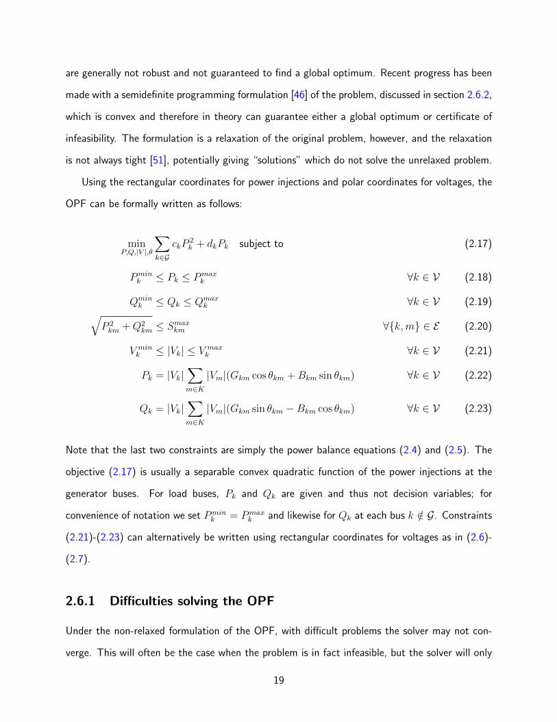
Using the rectangular coordinates for power injections and polar coordinates for voltages, the
OPF can be formally written as follows:
minP,Q,|V |,θ
∑k∈G
ckP2k + dkPk subject to (2.17)
Pmink ≤ Pk ≤ Pmax
k ∀k ∈ V (2.18)
Qmink ≤ Qk ≤ Qmax
k ∀k ∈ V (2.19)√P 2km +Q2
km ≤ Smaxkm ∀k,m ∈ E (2.20)
V mink ≤ |Vk| ≤ V max
k ∀k ∈ V (2.21)
Pk = |Vk|∑m∈K
|Vm|(Gkm cos θkm +Bkm sin θkm) ∀k ∈ V (2.22)
Qk = |Vk|∑m∈K
|Vm|(Gkm sin θkm −Bkm cos θkm) ∀k ∈ V (2.23)
Note that the last two constraints are simply the power balance equations (2.4) and (2.5). The
objective (2.17) is usually a separable convex quadratic function of the power injections at the
generator buses. For load buses, Pk and Qk are given and thus not decision variables; for
convenience of notation we set Pmink = Pmax
k and likewise for Qk at each bus k /∈ G. Constraints
(2.21)-(2.23) can alternatively be written using rectangular coordinates for voltages as in (2.6)-
(2.7).
2.6.1 Difficulties solving the OPF
Under the non-relaxed formulation of the OPF, with difficult problems the solver may not con-
verge. This will often be the case when the problem is in fact infeasible, but the solver will only
19
report that it encountered numerical difficulties or simply failed to converge. The solvers cannot
guarantee that the problem is infeasible. For some applications, such as the economic dispatch
problem, this may not be a huge issue: configurations of the grid where the OPF solver fails to
converge can all be considered “bad” and adjusted until it does converge. For other applications
(e.g. the attack problem in part II), lack of convergence is a problem because we do not know
whether the configuration of the grid being considered is truly vulnerable (the OPF is infeasible
– there is no possible power flow) or it is relatively harmless and the solver is just having trouble.
Another potential problem with the standard formulation of the OPF is that a solution found via
a local method may fail to be a global optimum. [22] includes many examples of OPF problems
with suboptimal local solutions.
Significant progress in the robustness of OPF solvers has been made recently, in particular
the semidefinite relaxation discussed in the next section. These new techniques have their own
drawbacks, however, and software implementations are not as mature. For this dissertation,
the OPF is an important building block of the attack problem in part II. We used the interior-
point solver IPOPT [66] which performs well in practice. For some small problems, we used the
semidefinite programming approach to obtain certificates of infeasibility. We use the OPF with
the DC approximation in part I for the economic dispatch problem; because the DC assumptions
make the problem linear, the difficulties described here do not arise. Section 2.7 describes some
specific examples of difficult OPF problems.
2.6.2 Semidefinite relaxation of the OPF
A recent development that has renewed interest in solution methods for the OPF is the semidef-
inite relaxation. It is a convex formulation of the problem, and thus has the potential to be
much more robust than conventional solution methods. In this section we introduce semidefi-
nite programming, and very briefly describe the semidefinite relaxation of the OPF as well as its
shortcomings. For a more thorough treatment, see e.g. [46–48, 51].
Semidefinite programming (SDP) is a method that optimizes a linear objective function over
20
the intersection of a cone of positive semidefinite matrices and an affine plane. SDP problems
are convex and can be efficiently solved with interior point methods. Some free software that can
solve SDPs include SeDuMi [63] and SDPT3 [64].
Denote by Sn the set of symmetric n×n matrices, and for two n×n matrices A and B, the
Frobenius inner product:
A •B = trace(AB) =n∑i=1
n∑j=1
AijBij
A general semidefinite program can be written as
minW∈Sn
C •W (2.24)
subject to Ai •W = bi, i = 1, ...,m (2.25)
W 0 (2.26)
where W is the matrix decision variable, C ∈ Sn is a given cost matrix, Ai ∈ Sn are given
constraint matrices with the constraint vector b ∈ Rm, and indicates that a matrix is positive
semidefinite.
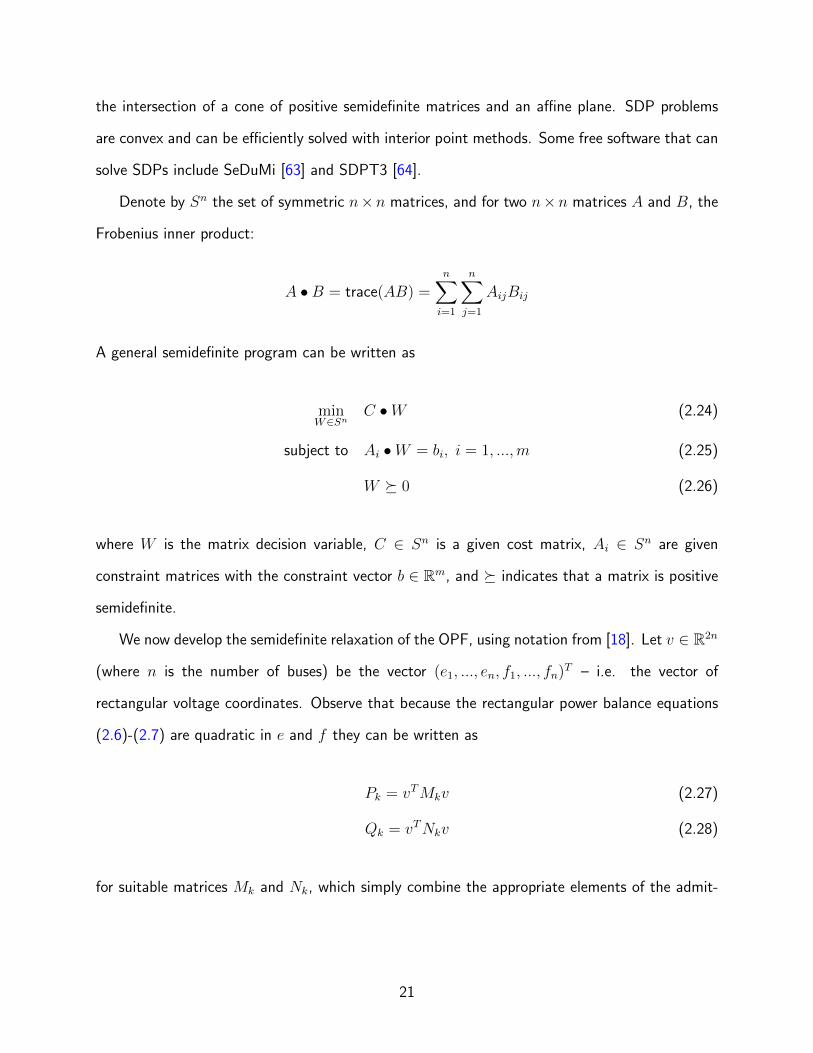
We now develop the semidefinite relaxation of the OPF, using notation from [18]. Let v ∈ R2n
(where n is the number of buses) be the vector (e1, ..., en, f1, ..., fn)T – i.e. the vector of
rectangular voltage coordinates. Observe that because the rectangular power balance equations
(2.6)-(2.7) are quadratic in e and f they can be written as
Pk = vTMkv (2.27)
Qk = vTNkv (2.28)
for suitable matrices Mk and Nk, which simply combine the appropriate elements of the admit-
21
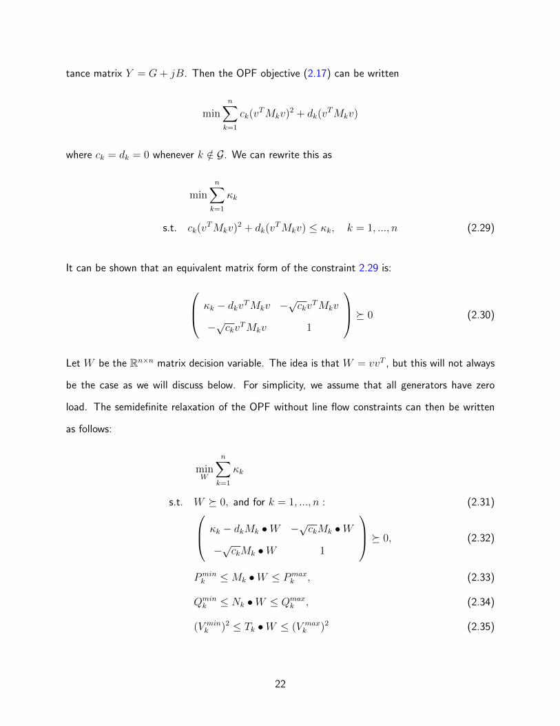
tance matrix Y = G+ jB. Then the OPF objective (2.17) can be written
minn∑k=1
ck(vTMkv)2 + dk(v
TMkv)
where ck = dk = 0 whenever k /∈ G. We can rewrite this as
minn∑k=1
κk
s.t. ck(vTMkv)2 + dk(v
TMkv) ≤ κk, k = 1, ..., n (2.29)
It can be shown that an equivalent matrix form of the constraint 2.29 is:
κk − dkvTMkv −√ckv
TMkv
−√ckvTMkv 1
0 (2.30)
Let W be the Rn×n matrix decision variable. The idea is that W = vvT , but this will not always
be the case as we will discuss below. For simplicity, we assume that all generators have zero
load. The semidefinite relaxation of the OPF without line flow constraints can then be written
as follows:
minW
n∑k=1
κk
s.t. W 0, and for k = 1, ..., n : (2.31) κk − dkMk •W −√ckMk •W
−√ckMk •W 1
0, (2.32)
Pmink ≤Mk •W ≤ Pmax
k , (2.33)
Qmink ≤ Nk •W ≤ Qmax
k , (2.34)
(V mink )2 ≤ Tk •W ≤ (V max
k )2 (2.35)
22

where Tk is a diagonal matrix with ones in position k and k + n and otherwise zero, so that
Tk • vvT = e2k + f 2
k . Including the line flow constraints requires a construction similar to that of
the other constraints.
If we replace the constraint W 0 with the rank-one constraint
W = vvT (2.36)
the formulation is exact and not a relaxation. Constraint 2.36 is not convex, however, and
thus cannot be enforced by an SDP solver. The semidefinite relaxation is tight if the global
optimum W happens to have rank one. This is the case for most practical instances of the
problem, and under a number of appropriate sufficient conditions [47, 48]. In general, however,
the relaxation can produce an optimum W with rank greater than one, and thus fail to produce
a meaningful solution v. Furthermore, the SDP relaxation can be feasible when the original OPF
is infeasible [44]. [51] and [22] include additional practical examples where the relaxation fails
because rank(W ) > 1.
Another significant drawback of the semidefinite approach is that it is much more compu-
tationally expensive: the number of decision variables increases from order n to order n2. In
practice, for large and complex grids the SDP formulation can be prohibitively slow to solve for
some applications. Progress continues to be made, however, and [45] describes other relaxations
of the OPF which are much faster to solve.
2.7 Difficult optimal power flow examples
To reinforce the difficulty of the OPF, this section will examine some problems which prove
troublesome for numerical solvers. We will provide examples for the following situations:
1. The solver converges to a non-optimal local solution
2. Two different solvers converge to two different solutions
23

~z=0.04+0.20j
[P1, Q1](|V1|, θ1)
[350, -350](|V2|, θ2)
1 2
Figure 2.5: Two bus grid from [22]. Note that we use the impedance z rather than the admittancey in this example.
3. The solver fails to converge after a very large number of iterations
2.7.1 Two-bus OPF with local solutions
Consider the two bus grid in Fig. 2.5 from [22]. There is a single generator at bus 1 and the
objective is to minimize the active power output. Voltage magnitude limits on each bus are set to
[.95, 1.05] and there are no line flow limits. This very simple OPF has a feasible region consisting
of two disconnected segments in the |V1| − |V2| plane. Setting the initial guess for a standard
OPF solver in one region results in the global optimum; starting in the other region leads to a
more costly local optimum. See Fig. 2.6.
Furthermore, as reported in [22], setting the voltage magnitude limit for bus 2 to a value
in the range [.977, 1.034] causes the SDP solver to fail. Conventional local solvers correctly
converge to the only remaining feasible optimum at (.95, .976) in this case.
2.7.2 Different solvers converge to different solutions
In the modification described in [22] to the nine bus grid case9 from MATPOWER [72], they
raise the reactive power generation bounds from -300 MVAR to -5 MVAR and scale all loads
by 60%. This gives rise to four local solutions. Solving this case with the trust region solver
TRALM from [68] results in the globally optimal solution. Solving it instead with the interior
point method PDIPM, also from [68], results in the worst of the four local solutions, which has
a cost 37% greater than the global optimum.
24
|V1|0.95 0.951 0.952 0.953 0.954 0.955
|V2|
0.94
0.96
0.98
1
1.02
1.04
1.06
438.9
449
458.5P1
Figure 2.6: Two bus example from [22]. Note that the set of feasible points (V1, V2) is discon-nected. Searching locally along the blue feasible region yields the non-optimal local solution at(.95, .976) marked with the dot. Searching in the red feasible region gives the global minimummarked by the star at (.952, 1.05).
.
25
2.7.3 Failure to converge after many iterations
This particular example comes from our investigation of the attack problem in part II. The 57-
bus grid in case57 from MATPOWER is modified so that the lines 35, 36, and 46 have their
impedance multiplied by 4. Line flow constraints are removed and voltage magnitude constraints
at load buses are relaxed to [.5, 1.5]. Voltage constraints at generators are set to ±1% of their
normal values.
At iteration 8017 and after over a minute of computation, IPOPT reports that it believes
the problem is infeasible. This required several iterations of increasing the maximum number of
iterations because the default maximum is set to 250, which works well for the vast majority of
problems. In contrast, the SDP solver reports the problem is infeasible in four seconds and 31
iterations. In the attack problem, small variations of this OPF are computed thousands of times
as a subroutine, usually converging in a fraction of a second. The performance of IPOPT for this
problem illustrates the difficulty of using the OPF as a subroutine with the current technology.
26
Part I
The economic dispatch problem
with uncertain power sources4
4Adapted from Chance-Constrained Optimal Power Flow: Risk-Aware Network Control under Uncertainty byDaniel Bienstock, Michael Chertkov, and Sean Harnett. SIAM Review 56 (2014) [19].
27
Chapter 3
Introduction
The smart grid – the use of computer-based control and automation technologies to manage
the increasing complexity of the modern power grid – is well on its way. A large motivation
for the smart grid and a major contributor to the increased complexity is our desire for greater
use of renewable energy. But the large-scale introduction of renewables brings with it the risk
of large, random variability. This is a condition that the current grid, built in the 1890s under
much simpler elecricity needs, was not developed to accommodate. Automatic grid control and
regulations achieve remarkable robustness of operation under normal fluctuations, in particular
under the forecasted inter-day demands. But as the size of power fluctuations grows, which it will
with increased renewable penetration, the automatic systems can fail and must rely on human
input to restore stability to the grid.
The economic dispatch problem (see section 2.6) is one example where greatly increased
renewable penetration creates challenges for the way the grid is currently operated. Economic
dispatch is used to set generator outputs over approximately 15-minute time windows so as to
meet demand at minimum cost, subject to transmission and operational constraints. Estimates
of the expected loads for the upcoming time window are employed in this computation. In real
time, the generator outputs computed by economic dispatch are modulated by the Automatic
Generation Control (AGC) system (see section 3.1) to account for variations in demand from
28
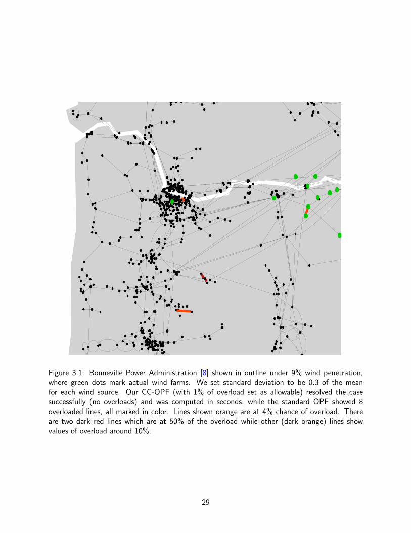
Figure 3.1: Bonneville Power Administration [8] shown in outline under 9% wind penetration,where green dots mark actual wind farms. We set standard deviation to be 0.3 of the meanfor each wind source. Our CC-OPF (with 1% of overload set as allowable) resolved the casesuccessfully (no overloads) and was computed in seconds, while the standard OPF showed 8overloaded lines, all marked in color. Lines shown orange are at 4% chance of overload. Thereare two dark red lines which are at 50% of the overload while other (dark orange) lines showvalues of overload around 10%.
29
the estimates. Because AGC does not respect transmission constraints, this scheme can fail
dramatically when renewables are part of the generation mix and fluctuations in their output
become large. Specifically, combinations of generator and renewable outputs can conspire to
produce power flows that significantly exceed transmission line ratings, increasing the chances
that those lines trip (see section 2.1). If several key lines trip, the grid is likely to become unstable
and experience a cascading failure, with large losses in served load. To prevent line tripping an
additional scheme is employed as a part of the current operational routine. It requires a human
operator in the loop and is based on direct line flow measurements: after receiving a warning,
the operator may initiate an emergency action, possibly disconnecting the overheated line.
The U.S. is committed to increasing the proportion of power delivered from renewable sources
[4] while safety margins (between typical power flows and line ratings) continue to shrink [42].
Without significant changes, line overloads will become much more frequent, and so the current
operational paradigm is most likely unsustainable. A possible failure scenario is illustrated in
figure 3.1 with U.S. Pacific Northwest regional grid data (2866 lines, 2209 buses, 176 generators
and 18 wind sources), where lines highlighted in red are jeopardized (flow becomes too high) with
unacceptably high probability by fluctuating wind resources positioned along the Columbia river
basin.
This part of the dissertation investigates a solution by explicitly modeling fluctuating power
sources in the economic dispatch problem. The non-deterministic behavior of wind make it
natural to cast the problem in terms of stochastic optimization. Recent works [16,26,27] suggest
that focusing on the most-likely dangerous events provides a practicable route to risk control
and assessment. The approach described here goes one step further, by implicitly discovering
probable realizations of line overloads and correcting them in a single step.
The particular type of stochastic optimization used in our approach is known as “chance-
constrained” optimization [54], which allows for constraints stating that the probability of a certain
random event is kept smaller than a target value. Our formulation of the problem minimizes the
average cost of generation over the random power injections (from renewables), while specifying
30
a mechanism by which the dispatchable generators adjust in real-time to compensate for the
power fluctuations, and guaranteeing a low probability that any line will exceed its rating. This
last constraint is naturally formulated as a chance constraint. The economic dispatch problem
is a particular type of optimal power flow problem (section 2.6) and though we examine only
economic dispatch, our method applies more generally to OPF problems. Thus we term our
approach Chance-Constrained Optimal Power Flow, or CC-OPF.
Part I of this dissertation is organized as follows. The remainder of this chapter motivates
and presents the various mathematical models used to describe how the grid operates, as well as
the proposed methodology. Chapter 4 explains how to solve the models. Chapter 5 then presents
a number of examples to demonstrate the speed and usefulness of our approach.
3.1 Transmission system controls
Transmission systems (see 2.1 for more background information) balance load and generation
using a complex strategy that spans three different time scales (see e.g. [17]). An essential
stability requirement is that all generators operate at the same frequency – 60Hz in the U.S.
Failure to maintain a common frequency leads to a loss of synchrony, and can force generators
to shut down for protective reasons, potentially leading to a swift collapse of the grid.
In real time, changes in loads are observed at generators by an opposite change in frequency.
Consider the case of a sudden load increase. In that case generator frequency will start to
drop. The so-called primary frequency control will react to stop frequency drift by having each
participating generator inject more power into the grid, proportionally to the frequency change.
This reaction is swift and local, leading to stabilization of frequency across the system, however
not necessarily at the nominal 60Hz value.
The task of the secondary, or Automatic Generation Control (AGC), is to undertake the
adjustment of generation levels to return frequency to 60Hz. The economic dispatch algorithm
typically runs as frequently as every 15 minutes providing information to the AGC, which ultimately
31
undertakes the adjustment of generation levels to achieve optimal (or close to optimal) control.
The economic dispatch time-window thus represents the shortest time scale where actual off-line
and network wide optimal computations are employed.
3.2 Standard generation dispatch
This section reviews and further describes the way power is usually dispatched, by means of a
conventional optimal power flow. We’ll refer to this scheme as simply “standard OPF”. Note:
to stay consistent with [19] we will use slightly different notation from the discussion in section
2.3: we’ll use fkm rather than Pkm for the power flow along line k,m, and βkm for susceptance
rather than bkm so that fkm = βkm(θk − θm).
The optimal power flow problem is introduced in section 2.6. We use the DC approximation
(section 2.4.2), so we ignore reactive power and voltage magnitude. We can informally describe
the DC-OPF problem as follows:
• The goal is to determine the vector of active power generated and voltage angles so as to
minimize a convex quadratic objective function of the generator power outputs
• There are three types of constraints: power flow, line limit, and generation bound con-
straints.
Let dk be demand (possibly zero) at bus k and pk the power generated (also possibly zero).
Then the power injected into the grid from bus k is pk − dk. With this notation, the DC power
flow equation in matrix form is
Bθ = p− d (3.1)
where recall that the susceptance matrix B is a weighted-Laplacian defined by Bkm = −βkm and
Bkk =∑
m∈Ωkβkm.
32
For future reference, we state some well known properties of Laplacians and the power flow
system (3.1).
Lemma 3.2.1. The following statements hold for the system (3.1):
• the sum of rows of B is zero
• if the underlying graph is connected, the rank of B is n− 1
• if (3.1) is feasible, then for any index k there is a solution with θk = 0
• the system (3.1) is feasible in θ if and only if total generation equals total demand
More formally, the standard DC-OPF problem can be stated as the following constrained
optimization problem:
DC-OPF: minp,θ
c(p), s.t. (3.2)
Bθ = p− d, (3.3)
∀k ∈ G : pmink ≤ pk ≤ pmaxk , (3.4)
∀k,m ∈ E : |βkm(θk − θm)| ≤ fmaxkm , (3.5)
Note that the pmink , pmaxk quantities can be used to enforce the convention pk = 0 for each k /∈ G;
if k ∈ G then pmink , pmaxk are lower and upper generation bounds which are generator-specific.
Constraint (3.5) is the line limit constraint for k,m; fmaxkm represents the line limit which is
assumed to be strictly enforced. This conservative condition will be relaxed in what follows.
Problem (3.2) is a convex quadratic program, easily solved using modern optimization tools.
The vector d of demands is fixed in this problem and is obtained through estimation. In practice,
however, demand will fluctuate around d; generators then respond by adjusting their output
(from the OPF-computed quantities) proportionally to the overall fluctuation as discussed above
in section 3.1. This scheme works well in current practice, since demands usually do not fluctuate
significantly over the approximately 15-minute time scale between OPF calculations.
33
3.3 Adjusting to power fluctuations
When fluctuations in power injections grow large, the scheme in the previous section can lead to
serious line overloads. This section examines more closely the details of how this happens, by
describing how generator output is modulated in real time to respond to changes in demand.
Suppose we have computed, using the standard OPF, the output pk for each generator k
assuming constant demands d. Let d(t) be the vector of real-time demands at time t, and
similarly p(t) the vector of real-time generator outputs. Then so-called “frequency control,” or
more properly, the combination of primary and secondary controls (section 3.1) will achieve (on
the scale of minutes) the following real-time generator outputs:
pk(t) = pk − ρk∑m
(dm − dm(t)) ∀k ∈ G (3.6)
In this equation, the quantities ρk ≥ 0 are fixed and satisfy∑
k ρk = 1. ρk represents the
proportional adjustment made by generator k to the mismatch between the forecasted and actual
demand. Taking the sum of (3.6) over all k, and assuming the system is feasible so that∑k pk =
∑k dk, we obtain
∑k
pk(t) =∑k
pk −∑m
(dm − dm(t)) =∑k
dk(t),
and thus the demand matches supply over time. The quantities ρk are generator dependent but
essentially chosen far in advance and without regard to short-term demand forecasts.
Generator outputs are set in this hierarchical fashion: the OPF computes a base level, and
then real-time adjustments are made according to (3.6) which is risk-unaware. This scheme has
worked in the past because of the slow time scales of change in uncontrolled resources (mainly
loads). That is to say, frequency control and load changes are well-separated. An error in the
forecast of d for the next – e.g., 15 minute – period may lead to an operational problem1. This is
1See for example the discussions in [3, 49]
34
because even though the vector p(t) suffices to meet average demands, the θ(t) computed from
Bθ(t) = p(t)− d(t)
may give rise to real-time power flows
fkm(t).= βkm[θk(t)− θm(t)]
that violate the line flow constraints (3.5). Even the generator constraints (3.4) may fail to hold.
This has not been considered a handicap since any resulting line trips are rare, primarily because
the deviations dk(t) − dk will be small in the time scale of interest. In effect, the risk-unaware
approach that assumes constant demands has worked well.
Now let us consider the case where demands are constant, but some generators have fluctu-
ating output.2 Let a subset W of the buses hold uncertain power sources (wind farms); for each
k ∈ W , write the amount of power generated by source k at time t as µk + ωk(t), where µk
is the forecast output of farm k in the time period of interest and ωk(t) is the fluctuation from
the forecast over time. For ease of exposition, we will assume in what follows that G refers to
the set of buses holding controllable generators, i.e. G ∩W = ∅. Renewable generation can be
incorporated into the OPF formulation (3.2)-(3.5) by simply setting pk = µk for each k ∈ W .
With constant demands and fluctuating power sources, the application of frequency control yields
the following analog to (3.6):
pk(t) = pk − ρk∑m∈W
ωm(t) ∀k ∈ G (3.7)
For instance, if∑
m∈W ωm(t) > 0, that is, there is a net increase in wind output, then (control-
lable) generator output will proportionally decrease.
Eq. (3.7) describes how generation will adjust to wind changes under current power engineering
2This is essentially a matter of notation, but we make the distinction because we will use the fluctuatinggenerator formulation in what follows.
35

practice. The hazard embodied in this relationship is that the quantities ωm(t) can be large,
resulting in changes in power flows significant enough to overload power lines. The risk of such
overloads can be expected to increase [42]; this is due to a projected increase of renewable
penetration in the future [4], accompanied by the decreasing gap between normal operation and
limits set by line capacities. Tightening the line flow limits can succeed in deterministically
preventing overloads, but it also forces excessively conservative choices of the generation re-
dispatch, with the potential risk of greatly increased cost and extreme volatility of the electricity
markets. See e.g. the discussion in [67] on abnormal price fluctuations in markets that are heavily
reliant on renewables.
3.4 Using chance constraints
Section 2.1 describes the nature of a line trip due to thermal overload – the result of carrying
too much power for too long. The failure does not necessarily happen instantly and is difficult
to model3 but a trip is more likely to occur the longer the line stays overheated.
So as an enhancement to the standard OPF which assumes static demand and power gen-
eration, we would ideally address the problem in the previous section by updating the static line
constraints (3.5) with constraints of the form “the fraction of the time that the line exceeds its
limit within a certain time window is small.” Direct implementation of this constraint would re-
quire resolving dynamics of the grid over the generator dispatch time window of interest. Instead
we propose the following static proxy of this ideal model – a chance constraint: we will require
that the probability that a given line exceeds its limit is small.
To formalize this notion, we assume:
1. For each k ∈ W , the (stochastic) amount of power generated by source k is of the form
µk + ωk, where
2. µk is constant, assumed known from the forecast, and ωk is a zero mean independent
3See [2] for discussions of line tripping during the 2003 Northeast U.S.-Canada blackout.
36
random variable with known standard deviation σk.
Here and in what follows, we use bold face to indicate uncertain quantities. For line k,m,
let a tolerance parameter εkm > 0 be given and recall that fkm is the (uncertain) flow. The
chance constraint for line k,m is then:
P (fkm > fmaxkm ) < εkm and P (fkm < −fmaxkm ) < εkm (3.8)
Likewise4, for a generator g we will require that
P (pg > pmaxg ) < εg and P (pg < pming ) < εg. (3.9)
The parameter εg will be chosen extremely small, so that for all practical purposes all generator
outputs will be guaranteed to stay within respective bounds.
Chance constraints [25, 50, 58] are but one possible methodology for handling uncertain data
in optimization. Broadly speaking, this methodology fits within the general field of stochastic
optimization. Constraint (3.8) can be viewed as a “value-at-risk” statement; the closely-related
“conditional value at risk” concept provides a (convex) alternative, which roughly stated con-
strains the expected overload of a line to remain small, conditional on there being an overload
(see [54] for definitions and details).
One alternative model would impose the much stronger constraint
P (∃ line k,m s.t. |fkm| > fmaxkm ) < ε, (3.10)
with a single global tolerance ε. Nemirovski and Shapiro [54] develop a general framework for
constructing, under appropriate assumptions, a convex optimization problem with an approximate
version of constraint (3.10).
4One could alternatively use the more conservative constraint P (|fkm| > fmaxkm ) < εkm. This implies (3.8),
and if (3.8) holds then P (|fkm| > fmaxkm ) < 2εkm. However, (3.8) proves more tractable, and moreover we are
interested in the regime where εkm is fairly small; thus we estimate that there is small practical difference betweenthe two constraints; this will be verified by our numerical experiments.
37
Reference [70] considers the standard OPF problem under stochastic demands, using chance
constraints to guarantee high probability that the system operates within acceptable bounds. The
problem is tackled using a simulation-based local optimization system, with experiments using a
5-bus and a 30-bus example.
Another related study [65] describes a scenario-based system for reserve scheduling with
fluctuating wind generation, using chance constraints to limit line or generator overloads. This
optimization is tackled via transformation to a convex problem and a heuristic scheme, with no
convergence to global optimum of the nonlinear problem guaranteed.
Chance constrained optimization has also been discussed recently in relation to the unit
commitment problem, which is used to plan the operation of large generation units on the scale
of hours-to-months, so as to account for long-term wind-farm generation uncertainty [56,69,71].
3.5 Uncertain power sources
In what follows, we assume that the outputs of the wind power sources vary between OPF
calculations as (1) independent (2) normally distributed random variables with (3) known mean
and variance. Let us examine the components of this assumption.
We assume that reasonably accurate, standard forecasts of wind speed for the next OPF time
window are available at a coarse-grained level of minutes and kilometers. Along with known
“power curves” for the wind turbines, which describe the relationship between wind speed and
power output, this provides a forecast of the power generated by each wind farm for the next
time period. This sort of forecast data is already widely used, so this is not a large assumption.
The possibility of forecast errors can be handled efficiently with the so-called ambiguous chance
contrained approach, which we describe in detail in [19]. This extends the formulation here, where
the forecasts are constant, by letting them vary within a fixed set. Furthermore, the out-of-sample
numerical simulations in section 5.5 suggest that the degradation in the chance constraints are
small when data errors are small, so that the solution from our approach is not especially sensitive
38
to errors in the wind forecasts.
The independence of wind power fluctuations5 at different sites can be justified by the fact
that the wind farms are sufficiently far away from each other. For the typical economic dispatch
time span of 15 minutes and typical wind speed of 10m/s, fluctuations at farms more than 10km
apart are not correlated.
The assumption that the power output of a wind farm over a 15 minute period varies according
to a normal distribution is less justified. We use it as a first approximation for the purpose
of simplicity and because the resulting optimization problem is particularly efficient. Though
once again, numerical experiments (section 5.5) suggest that the errors due to non-normal wind
fluctuations are relatively small. The distribution of short-term (e.g. ten minute) average wind
speed observations over long time periods is well-researched [52], and the Weibull distribution
is commonly proposed as a good fit. In other words, there is a lot of data available for the
distribution of µk over a long period of OPF time windows. But our problem is concerned rather
with the fluctuations of wind speed from the forecasted value – ωk – on even shorter time scales.
Furthermore, we are concerned with wind power rather than speed, so turbine power curves
must be taken into account. Techniques exist6 to enable distributions other than the normal
distribution in our methodology, but at the cost of increased complexity. Future work on this
problem should revisit this assumption of normally distributed wind power fluctuations.
3.6 Affine Control
Since the power injections at each bus are fluctuating, we need a control scheme to ensure that
generation is equal to demand at all times within the time window of interest. We assume
that all governors involved in the controls respond to fluctuations in the generalized load (actual
demand which is assumed frozen minus stochastic wind resources) in a proportional way, however
5We assume that the fluctuations ωk are independent. Of course the overall wind levels in a region can becorrelated, which will be reflected in the forecasts of the average wind power µk.
6Chebyshev’s inequality is a rather crude technique, and there are more advanced methods from robust opti-mization [54].
39
with possibly different proportionality coefficients. Thus, we term the joint result of the primary
frequency control and secondary frequency control the affine control. The stochastic version of
Eq. (3.7) thus becomes
pk = pk − αk∑m∈W
ωm ∀k ∈ G : (3.11)
Here the quantities pk ≥ 0 and αk ≥ 0 are design variables satisfying (among other constraints)∑k∈G αk = 1. Thus the generator output pk combines a fixed term pk and a term which varies
with wind, −αk∑
m∈W ωm. Observe that∑
k pk =∑
k pk −∑
mωm, that is, the total power
generated equals the average production of the generators minus any additional wind power above
the average case.
Allowing α to change does not reflect current practice. We allow this degree of freedom
because (a) control of α is available, in principle; (b) we do not set any αk to a standard (fixed)
value, but instead leave it to the optimization to decide the optimal value; and (c) the freedom
is optional in that our formulation allows for linear constraints on α, so that it can be fixed if
desired. (In some cases it may even be advantageous to allow negative αk but we decided not to
consider such a drastic change of current policy in this study.)
This affine control scheme creates the possibility of requiring a generator to produce power
beyond its limits. With unbounded wind, this possibility is inevitable, though we can restrict it
to occur with arbitrarily small probability, which we will do with additional chance constraints for
all controllable generators, ∀g ∈ G,
P (pming ≤ pg − αg∑k∈W
wk ≤ pmaxg ) > 1− εg. (3.12)
3.7 Overview of the CC-OPF solution methodology
Our methodology applies and develops general ideas on chance-constrained optimization [54] to
the setting of the OPF under uncertainty. In section 4.1 we will provide a generic formulation of
40
our chance-constrained OPF problem that is valid under the assumption of linear power flow laws
and statistical independence of wind fluctuations at different sites, while using control law (3.11)
to specify standard generation response to wind fluctuations. Under the additional assumption
that the fluctuations are normally distributed, in section 4.2 this formulation is reduced to a
deterministic convex optimization problem, more precisely, a second-order cone program (SOCP)
[21, 35]; an efficient computational implementation is discussed in section 4.3.
Many of our assumptions are not restrictive and allow natural generalizations. Using tech-
niques from [54], one can relax the assumption of normally distributed wind sources. For example,
using only the mean and variance of output at each wind farm, one can use Chebyshev’s inequal-
ity to obtain a similar though more conservative formulation. And following [54] one can also
obtain convex approximations to (3.8) which are tighter than Chebyshev’s inequality, for a large
number of empirical distributions discussed in the literature. The data-robust version of our algo-
rithm discussed in [19] provides a methodologically sound (and computationally efficient) means
to protect against data and model errors. Additionally out-of-sample experiments (section 5.5)
involving the controls computed with the nominal approach (first to investigate the effect of
parameter estimation errors in the normally distributed case, and, second, to gauge the impact
of non-normal wind distributions) indicate robustness.
41
Chapter 4
Solving the chance-constrained OPF
problem
In this chapter we first formally describe the chance-constrained optimal power flow. We then
make use of the simplifying assumptions from section 3.5 to convert the chance constraints
(which include probability statements) into a form usable by optimization software. The resulting
convex optimization problem, though efficiently solvable in theory, raises numerical difficulties
for off-the-shelf optimization algorithms on large grids. In the final section we describe a simple
procedure to overcome the numerical difficulties and quickly solve the the CC-OPF on real grids
with thousands of buses and lines.
4.1 Chance-constrained optimal power flow: formal ex-
pression
Recall that we assume each wind source k produces power of the form µk + ωk, where µk
is constant and ωk1 is a zero mean independent random variable with standard deviation σk.
Eqs. (3.11) explain the affine control, where the αk are decision variables which control the
1Further recall that variables in bold denote random/fluctuating quantities.
42
proportional response of each generator to the total difference in power from the forecast. We
also use the usual power output decision variables pk, which the standard OPF (3.2) uses as well.
In our case, the bar indicates that these are the average power outputs, representing what would
be generated in the case where the wind did not fluctuate at all from the forecasted average.
4.1.1 Preliminaries
For convenience of notation, we let every bus have a wind power source but set the wind power
to zero for the other buses. Formally, where n is the number of buses, for k /∈ W we write
µk = σk = 0 (so that ωk = 0), thereby obtaining vectors µ, σ, ω ∈ Rn. Likewise, we extend p
and α to vectors in Rn by writing pk = αk = 0 whenever k /∈ G.
Definition. We say that the pair p, α is viable if the generator outputs under control law (3.11)
exactly match total demand under any configuration of uncertain outputs.
The following simple result characterizes this condition as well as other basic properties of
the affine control. Here and below, e ∈ Rn is the vector of all ones.
Lemma 4.1.1. Under the control law (3.11) the net output of bus k equals
pk + µk − dk + ωk − αk(eTω), (4.1)
and thus the (stochastic) power flow equations can be written as
Bθ = p+ µ− d+ ω − (eTω)α. (4.2)
Consequently, the pair p, α is viable if and only if
∑k∈V
(pk + µk − dk) = 0, (4.3)
∑k
αk = 1.
43
Proof. Eq. (4.1) follows by definition of the p, µ, d vectors and the control law. Thus Eq. (4.2)
holds. By Lemma 3.2.1 from Eq. (4.2) one gets that p, α is viable iff
0 =n∑k=1
(pk − (eTω)αk + µk + ωk − dk)
=∑k
(pk + µk − dk),
since by construction∑
k αk = 1.
Equation (4.3) can be interpreted as stating the condition that expected total generation
must equal total demand; however the Lemma contains a rigorous proof of this fact.
Because the admittance matrix B is singular with rank n− 1, it is conventional to eliminate
the row corresponding to the slack bus and the column corresponding to the reference angle bus
to obtain a system with a unique solution. Our formulation does not include a single slack bus,
but rather every bus with αk > 0 is used to balance power fluctuations. For convenience we will
assume that bus n is the reference bus, and furthermore neither a generator nor a wind farm
bus, that is to say, n /∈ G ∪ W . We denote by B the invertible submatrix obtained from B by
removing row and column n, and write
B =
B−1 0
0 0
. (4.4)
We will use B as a sort of pseudoinverse of B. By Lemma 3.2.1 we can assume without loss of
generality that θn = 0. The following simple result will be used in what follows.
Lemma 4.1.2. Suppose the pair p, α is viable. Then under the control law (3.11) a vector of
(stochastic) phase angles is
θ = θ + B(ω − (eTω)α), where (4.5)
θ = B(p+ µ− d). (4.6)
44
As a consequence,
Eω[θ] = θ, (4.7)
and given any line k,m,
Eω[fkm] = βkm(θk − θm). (4.8)
Furthermore, each quantity θk or fkm is an affine function of the random variables ωk.
Proof. For convenience we rewrite system (4.2): Bθ = p + µ − d + ω − (eTω)α. Since p, α
is viable, this system is always feasible, and since the sum of rows of B is zero, its last row is
redundant. Therefore Eq. (4.5) follows since θn = 0, and Eq. (4.7) holds since ω has zero mean.
Since fkm = βkm(θk − θm) for all k,m, Eq. (4.8) holds. From this fact and Eq. (4.5) it
follows that θ and f are affine functions of ω.
4.1.2 Formal expression
Using this result we can now give an initial formulation to our chance-constrained problem.
Because this formulation includes probability statements, it is not directly usable by optimization
software. In the next section we will use the assumptions from section 3.5 to transform this to a
45
conventional convex optimization formulation.
CC-OPF: min Eω
[c(p− (eTω)α)
](4.9)
s.t.∑g∈G
αg = 1, α ≥ 0, p ≥ 0, (4.10)
∑k∈V
(pk + µk − dk) = 0, (4.11)
Bθ = p+ µ− d; (4.12)
for all lines k,m:
P(βkm(θk − θm + [B(ω − (eTω)α)]k − [B(ω − (eTω)α)]m ) > fmaxkm
)< εkm, (4.13)
P(βkm(θk − θm + [B(ω − (eTω)α)]k − [B(ω − (eTω)α)]m ) < −fmaxkm
)< εkm; (4.14)
for all generators g:
P(pg − (eTω)αg > pmaxg
)< εg and P
(pg − (eTω)αg < pming
)< εg. (4.15)
The variables in this formulation are p, α, and θ. Constraint (4.10) simply states basic conditions
needed by the affine control. Constraint (4.11) is (4.3). Constraints (4.12), (4.13) and (4.14)
express our chance constraint, in view of Lemma 4.1.2.
4.1.3 Objective
The objective function is the expected cost incurred by the stochastic generation vector
p = p− (eTω)α
over the varying wind power output w. In standard power engineering practice generation cost is
convex, quadratic and separable, i.e. for any vector p, c(p) =∑
k ck(pk) where each ck is convex
quadratic. Note that for any g ∈ G we have
p2g = p2
g + (eTω)2α2g − 2eTωpgαg,
46
from which we obtain, since the ωg have zero mean,
Ew[p2g] = p2
g + var(Ω)α2g,
where “var” denotes variance and Ω.=∑
k ωk. It follows that the objective function can be
written as
Eω[c(p)] =∑g∈G
cg2(p2g + var(Ω)α2
g
)+ cg1pg + cg0
(4.16)
where cg2 ≥ 0 for all g ∈ G. Consequently the objective function is convex quadratic, as a
function of p and α.
4.1.4 Variance of the line flow fkm
The above formulation is the formal statement for our optimization problem. Even though its
objective is convex in cases of interest, the formulation is not in a form that can be readily
exploited by standard optimization algorithms. Below we will provide an efficient approach to
solve relevant classes of problems with the above form; prior to that we need a technical result.
We will employ the following notation:
• For 1 ≤ k,m ≤ n let πkm denote the k,m entry of the matrix B given above, that is,
πkm =
[B−1]km, k < n,
0 otherwise.(4.17)
• Given α, for 1 ≤ k ≤ n write
δk.= [Bα]k =
n−1∑m=1
πkmαm, k < n,
0 otherwise.
(4.18)
We use π as simpler notation for B, and δ is the “solution” to the system Bδ = α using the
47
pseudoinverse B.
Lemma 4.1.3. Assume that the ωk are independent random variables. Given α, for any line
k,m,
var(fkm) = β2km
∑l∈W
σ2l (πkl − πml − δk + δm)2. (4.19)
Proof. Using fkm = βkm[θk − θm] and eq. (4.5) we have that
fkm − Eω[fkm] = βkm([B(ω − (eTω)α)]k − [B(ω − (eTω)α)]m)
= βkm
([Bω]k − [Bω]m − (eTω)δk + (eTω)δm
)= βkm
∑l∈W
(πkl − πml − δk + δm)ωl,
since by convention ωk = 0 for any k /∈ W . The result now follows.
Remark. Lemma 4.1.3 holds for any distribution of the ωk so long as independence is assumed.
Similar results are easily obtained for higher-order moments of the fkm.
4.2 Formulating the chance-constrained problem as a conic
program
In deriving the above formulation (4.9)-(4.15) for the CC-OPF we assumed that the ωk random
variables have zero mean. To obtain an efficient solution procedure we will additionally assume
that they are (a) independent and (b) normally distributed, as described in section 3.5. Under
these additional assumptions, since the fkm are affine functions of the ωk, there is a simple
restatement of the chance-constraints (4.13), (4.14), and (4.15) in a computationally practicable
form. See [54] for a general treatment of linear inequalities with stochastic coefficients. For any
real 0 < r < 1 we write η(r) = Φ−1(1 − r), where Φ is the cumulative distribution function of
the standard normal distribution.
48
Lemma 4.2.1. Let p, α be viable. Assume that the ωk are normally distributed and independent.
Then the following hold:
• For any line k,m, P (fkm > fmaxkm ) < εkm and P (−fkm > fmaxkm ) < εkm iff
βkm|θk − θm| ≤ fmaxkm − η(εkm)
[β2km
∑l∈W
σ2l (πkl − πml − δk + δm)2
]1/2
(4.20)
where as before θ = B(p+ µ− d) and δ = Bα.
• For any generator g, P(pg − (eTω)αg > pmaxg
)< εg and P
(pg − (eTω)αg < pming
)< εg
iff
pming + η(εg)
(∑k∈W
σ2k
)1/2
≤ pg ≤ pmaxg − η(εg)
(∑k∈W
σ2k
)1/2
. (4.21)
Proof. By Lemma 4.1.2, fkm is an affine function of the ωk; under the assumption it follows
that fkm is itself normally distributed. Thus, P (fkm > fmaxkm ) < εkm iff
Eω[fkm] + η(εkm) var(fkm) ≤ fmaxkm , (4.22)
and similarly, P (fkm < −fmaxkm ) < εkm iff
Eω[fkm]− η(εkm) var(fkm) ≥ −fmaxkm . (4.23)
Lemma 4.1.2 gives Eω[fkm] = βkm(θk−θm) while by Lemma 4.1.3, var(fkm) = β2km
∑l∈W σ
2l (πkl−
πml − δk + δm)2. Substituting these values into (4.22) and (4.23) yields (4.20). The proof of
(4.21) is similar.
Remark. Eq. (4.20) highlights the difference between e.g. our chance constraint for lines, which
requires that P (fkm > fmaxkm ) < εkm and that P (fkm < −fmaxkm ) < εkm, and the stricter
requirement that P (|fkm| > fmaxkm ) < εkm which amounts to
P (fkm > fmaxkm ) + P (fkm < −fmaxkm ) < εkm. (4.24)
49
Unlike our requirement, which is captured by (4.20), the stricter condition (4.24) does not admit
a compact statement.
We can now present a formulation of our chance-constrained optimization as a convex opti-
mization problem, on variables p, α, θ, δ, and s. We will assume in what follows that for all lines
k,m, εkm < 1/2, so that η(εkm) > 0.
min∑k∈G
ck2
(p2k + α2
k
∑m
σ2m
)+ ck1pk + ck0
; (4.25)
for 1 ≤ k ≤ n− 1 :n−1∑m=1
Bkm δm = αk; (4.26)
for 1 ≤ k ≤ n− 1 :n−1∑m=1
Bkmθm − pk = µk − di; (4.27)
∑k
αk = 1, α ≥ 0, p ≥ 0; (4.28)
pn = αn = δn = θn = 0; (4.29)
βkm|θk − θm|+ βkmη(εkm) skm ≤ fmaxkm ∀ k,m; (4.30)[∑l∈W
σ2l (πkl − πml − δk + δm)2
]1/2
− skm ≤ 0 ∀ k,m; (4.31)
−pg + η(εg)
(∑k∈W
σ2k
)1/2
≤ −pming ∀ g ∈ G; (4.32)
pg + η(εg)
(∑k∈W
σ2k
)1/2
≤ pmaxg ∀ g ∈ G; (4.33)
In this formulation, the variables skm are auxiliary and introduced to facilitate the discussion
below – since η(εkm) ≥ 0 without loss of generality (4.31) will hold as an equality. Constraints
(4.31), (4.32), and (4.33) are second-order cone inequalities [21]. A problem of the above form is
solvable in polynomial time using well-known methods of convex optimization; several commercial
software tools such as CPLEX [6], Gurobi [10], MOSEK [7] and others are available. Constraint
(4.26) is equivalent to δk =∑n−1
1=m πkmαm (as we did in (4.18)), however the πkm can be seen
50
to be all nonzero, whereas B is very sparse for typical grids. Constraint (4.31) can be relatively
dense – the sum has a term for each wind farm. As a percentage of the total number of buses,
however, this can be expected to be small.
4.3 Solving the conic program
Even though optimization theory guarantees that the above problem is efficiently solvable, ex-
perimental testing shows that in the case of large grids (thousands of lines) the problem proves
challenging. For example, in the Polish 2003-2004 winter peak case,2 we have 2746 buses, 3514
lines and 8 wind farms, and CPLEX [6] reports (after pre-solving) 36625 variables and 38507
constraints, of which 6242 are conic. On this problem, a recent version of CPLEX on a modern
workstation3 ran for 3392 seconds and was unable to produce a feasible solution. On the same
problem Gurobi reported “numerical trouble” after 31.1 cpu seconds and stopped.
In fact, all of the commercial solvers [6, 7, 10] we experimented with reported numerical
difficulties with problems of this size. Anecdotal evidence indicates that the primary cause for
these difficulties is not simply the size, but also to a large degree numerics in particular poor
conditioning due to the entries in the matrix B. These are susceptances, which are inverses of
reactances, and often take values in a wide range.
To address this issue we implemented an effective algorithm for solving problem (4.25)-(4.33).
For brevity we will focus on constraints (4.31) ((4.32) and (4.33) are similarly handled). For a
line k,m define
Ckm(δ).=
(∑l∈W
σ2l (πkl − πml − δk + δm)2
)1/2
.
Constraint (4.31) can thus be written as Ckm(δ) ≤ skm. For completeness, we state the following
result:
2Available with MATPOWER [72]3A machine with two Intel Xeon CPU X5570 2.93GHz chips (total of 8 cores) and 64GB RAM. CPLEX ran
on 16 parallel threads, making use of “hyperthreading.”
51
Lemma 4.3.1. Constraint (4.31) is equivalent to the infinite set of linear inequalities
Ckm(δ) +∂Ckm(δ)
∂δk(δk − δk) +
∂Ckm(δ)
∂δm(δm − δm) ≤ skm, ∀δ ∈ Rn (4.34)
Constraints (4.34) express the outer envelope of the set described by (4.31) [21]. Any vector
δ ∈ Rn which satisfies (4.31) (for a given choice of skm) is guaranteed to satisfy (4.34). Thus
a finite subset of the inequalities (4.34), used instead of (4.31), will give rise to a relaxation of
the optimization problem and thus a lower bound on the optimal objective value. Given Lemma
4.3.1 there are two ways to proceed, both motivated by the observation that at δ∗ ∈ Rn, the
most constraining inequality from among the set (4.34) (that is to say, the one whose left-hand
side evaluated at δ∗ is largest) is that obtained by choosing δ = δ∗.
First, one can use inequalities (4.34) as cutting-planes in the context of the ellipsoid method
[36], obtaining a polynomial-time algorithm. A different way to proceed yields a numerically
practicable algorithm, described below. For a classical reference, see [40]. Denote by F (p, α) the
objective function in Eq. (4.25).
Algorithm 4.1: Cutting plane procedure
The linear “master” system A(p, α, δ, θ, s)T ≥ b is defined to include constraints
(4.26)-(4.30)
Iterate
1 Set (p∗, α∗, δ∗, θ∗, s∗)← argminF (p, α) : A(p, α, δ, θ, s)T ≥ b
2 if all conic constraints are satisfied by (p∗, α∗, δ∗, θ∗, s∗) then Stop
3 else if all chance constraints are satisfied by (p∗, α∗) then Stop
4 Add to the master system the outer inequality (4.34) arising from the constraint
(4.31) which is most violated
End
As the algorithm iterates the master system represents a valid relaxation of the conic program
(4.26)-(4.31); thus the objective value of the solution computed in Step 1 is a valid lower bound
52
on the value of problem. Each problem solved in Step 1 is a linearly constrained, convex quadratic
program. Computational experiments involving large-scale realistic cases show that the algorithm
is robust and rapidly converges to an optimum.
Note that Step 3 is not redundant. Recall that our formulation includes the variables skm;
each such variable is lower bounded (via equation (4.31)) by the variance of flow on line k,m.
However in the cutting-plane algorithm we do not make explicit use of equation (4.31) – indeed,
we progressively approximate it by means of cutting planes. At a typical intermediate iteration
the current solution will still fail to satisfy (4.31), i.e. we may have, for some line (or lines)
k,m, [∑l∈W
σ2l (πkl − πml − δ∗k + δ∗m)2
]1/2
> s∗km, (4.35)
(where “*” indicates the current values of the variables) which would normally indicate that the
algorithm has not terminated because condition (4.31) has not been adequately represented by
the cutting-planes. However, in later stages of the algorithm it may be the case that (4.35) holds
for some lines, and yet the pair (p∗, α∗) already satisfies the chance constraints for all lines. This
situation will arise if in the current solution some of the s∗km quantities are artificially low, that is
to say, they could be increased so as to match the left-hand side of (4.35) without jeopardizing
feasibility of the rest of the solution, that is to say, constraint (4.30). The underlying dynamic
is that the conic constraints (4.31) are still somewhat loosely (outer-)approximated by a set of
linear inequalities, resulting in a range of possible values for a particular variable skm. One such
value will be picked by the underlying optimization solver; and as just argued this value may be
artificially low. A direct way to check that (p∗, α∗) satisfies the chance constraint for a given line
k,m, is straightforward – the flows fkm are normally distributed (as noted in Lemma 4.2.1)
and their means and variances can be directly computed from (p∗, α∗), and so we can directly
compute the probability that, under (p∗, α∗), any given fkm exceeds its corresponding line limit
(additionally, this procedure computes said probability, a useful output parameter). If (p∗, α∗)
indeed satisfies all chance constraints, it is optimal, since it attains a cost that matches a lower
53
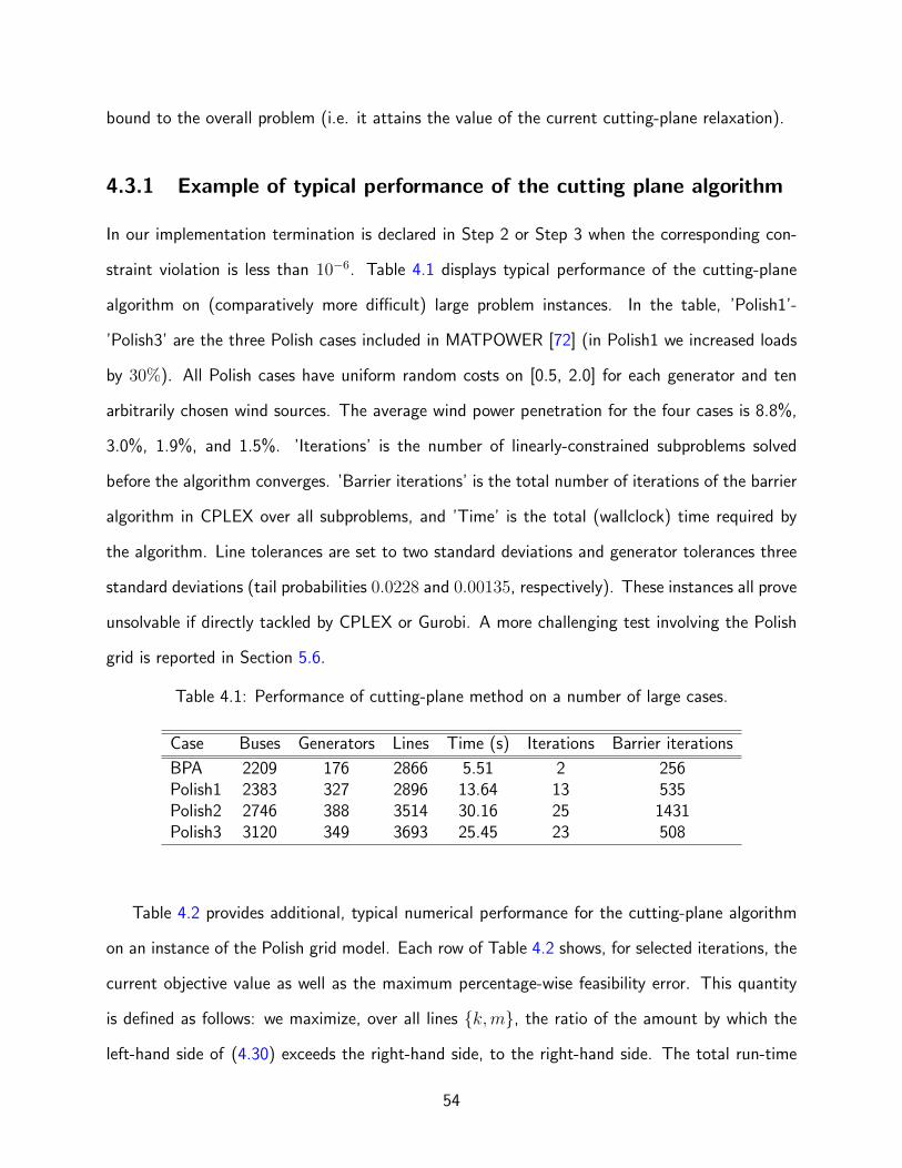
bound to the overall problem (i.e. it attains the value of the current cutting-plane relaxation).
4.3.1 Example of typical performance of the cutting plane algorithm
In our implementation termination is declared in Step 2 or Step 3 when the corresponding con-
straint violation is less than 10−6. Table 4.1 displays typical performance of the cutting-plane
algorithm on (comparatively more difficult) large problem instances. In the table, ’Polish1’-
’Polish3’ are the three Polish cases included in MATPOWER [72] (in Polish1 we increased loads
by 30%). All Polish cases have uniform random costs on [0.5, 2.0] for each generator and ten
arbitrarily chosen wind sources. The average wind power penetration for the four cases is 8.8%,
3.0%, 1.9%, and 1.5%. ’Iterations’ is the number of linearly-constrained subproblems solved
before the algorithm converges. ’Barrier iterations’ is the total number of iterations of the barrier
algorithm in CPLEX over all subproblems, and ’Time’ is the total (wallclock) time required by
the algorithm. Line tolerances are set to two standard deviations and generator tolerances three
standard deviations (tail probabilities 0.0228 and 0.00135, respectively). These instances all prove
unsolvable if directly tackled by CPLEX or Gurobi. A more challenging test involving the Polish
grid is reported in Section 5.6.
Table 4.1: Performance of cutting-plane method on a number of large cases.
Case Buses Generators Lines Time (s) Iterations Barrier iterations
BPA 2209 176 2866 5.51 2 256Polish1 2383 327 2896 13.64 13 535Polish2 2746 388 3514 30.16 25 1431Polish3 3120 349 3693 25.45 23 508
Table 4.2 provides additional, typical numerical performance for the cutting-plane algorithm
on an instance of the Polish grid model. Each row of Table 4.2 shows, for selected iterations, the
current objective value as well as the maximum percentage-wise feasibility error. This quantity
is defined as follows: we maximize, over all lines k,m, the ratio of the amount by which the
left-hand side of (4.30) exceeds the right-hand side, to the right-hand side. The total run-time
54
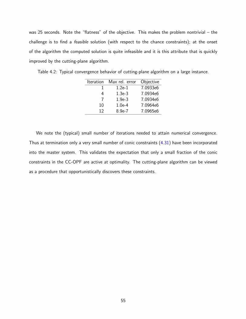
was 25 seconds. Note the “flatness” of the objective. This makes the problem nontrivial – the
challenge is to find a feasible solution (with respect to the chance constraints); at the onset
of the algorithm the computed solution is quite infeasible and it is this attribute that is quickly
improved by the cutting-plane algorithm.
Table 4.2: Typical convergence behavior of cutting-plane algorithm on a large instance.
Iteration Max rel. error Objective1 1.2e-1 7.0933e64 1.3e-3 7.0934e67 1.9e-3 7.0934e6
10 1.0e-4 7.0964e612 8.9e-7 7.0965e6
We note the (typical) small number of iterations needed to attain numerical convergence.
Thus at termination only a very small number of conic constraints (4.31) have been incorporated
into the master system. This validates the expectation that only a small fraction of the conic
constraints in the CC-OPF are active at optimality. The cutting-plane algorithm can be viewed
as a procedure that opportunistically discovers these constraints.
55
Chapter 5
Numerical experiments
Here we will describe qualitative aspects of our affine control on small systems; in particular
we focus on the contrast between the standard OPF and the CC-OPF on problematic features
that can arise because of fluctuating wind sources and on out-of-sample testing of the CC-OPF
solution, including the analysis of non-normal distributions. Some of our tests involve the BPA
grid and the Polish grid, which are large; we present additional sets of tests to address the
scalability of our solution methodology to the large cases.
Above (see Eq. (3.2)) we introduced the so-called standard OPF method for setting traditional
generator output levels. When renewables are present, the natural extension of this approach
would make use of some fixed estimate of output (e.g. mean output) and to handle fluctuations
in renewable output through the same method used to deal with changes in load: ramping output
of traditional generators up or down in proportion to the net increase or decrease in renewable
output. This feature could seamlessly be handled using today’s control structure, with each
generator’s output adjusted at a fixed (preset) rate. For the sake of simplicity, in the experiments
below we assume that all ramping rates are equal. That is, αg = 1/ng ∀g ∈ G where ng is the
number of generators.
Different assumptions on these fixed rates will likely produce different numerical results; how-
ever, this general approach entails an inherent weakness. The key point here is that mean
56
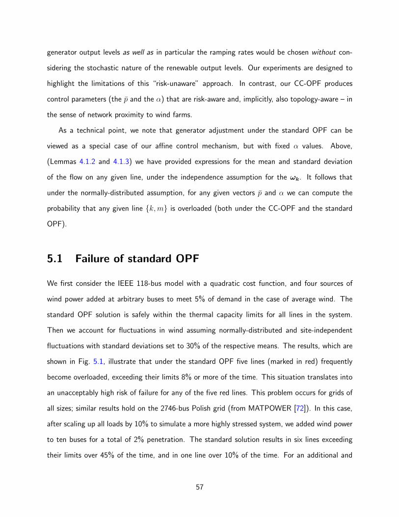
generator output levels as well as in particular the ramping rates would be chosen without con-
sidering the stochastic nature of the renewable output levels. Our experiments are designed to
highlight the limitations of this “risk-unaware” approach. In contrast, our CC-OPF produces
control parameters (the p and the α) that are risk-aware and, implicitly, also topology-aware – in
the sense of network proximity to wind farms.
As a technical point, we note that generator adjustment under the standard OPF can be
viewed as a special case of our affine control mechanism, but with fixed α values. Above,
(Lemmas 4.1.2 and 4.1.3) we have provided expressions for the mean and standard deviation
of the flow on any given line, under the independence assumption for the ωk. It follows that
under the normally-distributed assumption, for any given vectors p and α we can compute the
probability that any given line k,m is overloaded (both under the CC-OPF and the standard
OPF).
5.1 Failure of standard OPF
We first consider the IEEE 118-bus model with a quadratic cost function, and four sources of
wind power added at arbitrary buses to meet 5% of demand in the case of average wind. The
standard OPF solution is safely within the thermal capacity limits for all lines in the system.
Then we account for fluctuations in wind assuming normally-distributed and site-independent
fluctuations with standard deviations set to 30% of the respective means. The results, which are
shown in Fig. 5.1, illustrate that under the standard OPF five lines (marked in red) frequently
become overloaded, exceeding their limits 8% or more of the time. This situation translates into
an unacceptably high risk of failure for any of the five red lines. This problem occurs for grids of
all sizes; similar results hold on the 2746-bus Polish grid (from MATPOWER [72]). In this case,
after scaling up all loads by 10% to simulate a more highly stressed system, we added wind power
to ten buses for a total of 2% penetration. The standard solution results in six lines exceeding
their limits over 45% of the time, and in one line over 10% of the time. For an additional and
57
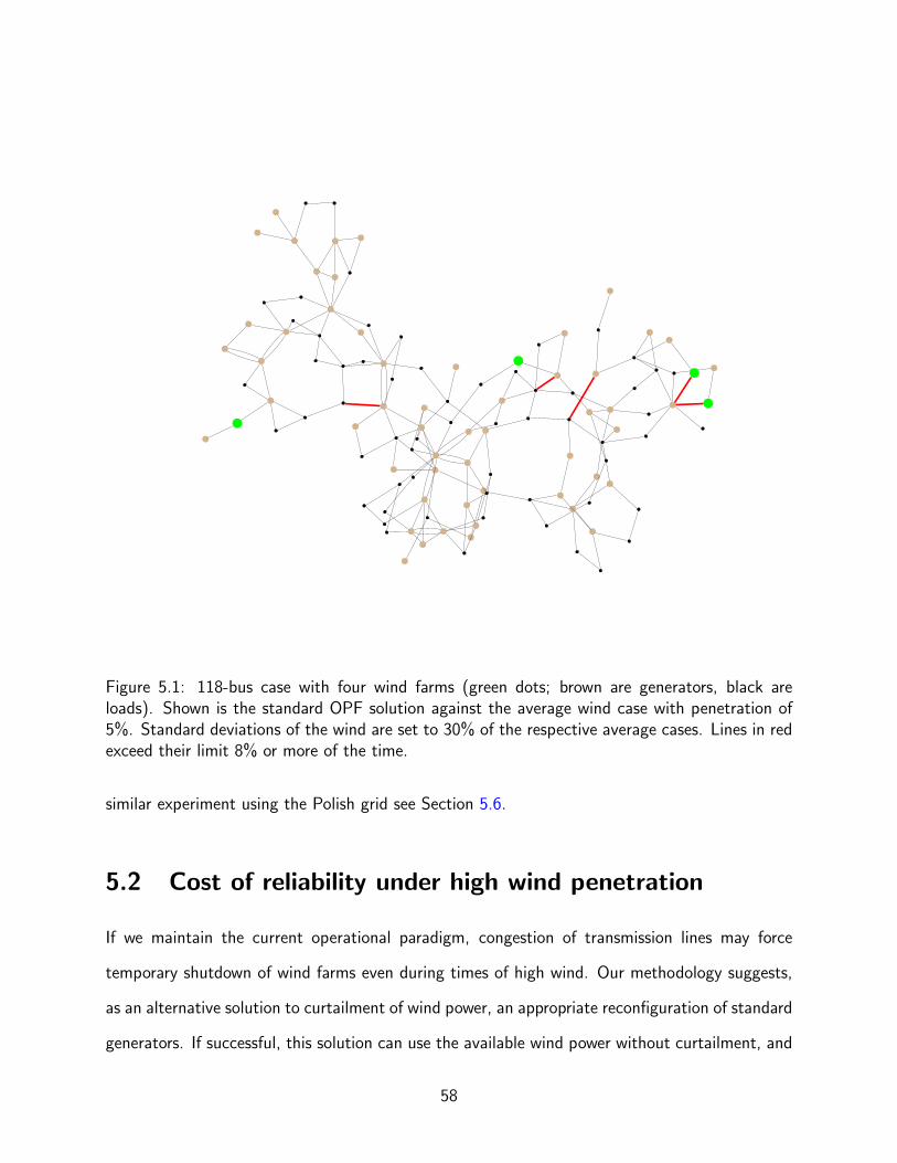
Figure 5.1: 118-bus case with four wind farms (green dots; brown are generators, black areloads). Shown is the standard OPF solution against the average wind case with penetration of5%. Standard deviations of the wind are set to 30% of the respective average cases. Lines in redexceed their limit 8% or more of the time.
similar experiment using the Polish grid see Section 5.6.
5.2 Cost of reliability under high wind penetration
If we maintain the current operational paradigm, congestion of transmission lines may force
temporary shutdown of wind farms even during times of high wind. Our methodology suggests,
as an alternative solution to curtailment of wind power, an appropriate reconfiguration of standard
generators. If successful, this solution can use the available wind power without curtailment, and
58
thus result in cheaper operating costs.
As a (crude) proxy for curtailment, we perform the following experiment, which considers
different levels of renewable penetration. Here, the mean power outputs of the wind sources are
kept in a fixed proportion to one another and proportionally scaled so as to vary total amount of
penetration, and likewise with the standard deviations. Under a high penetration level (e.g. 30%),
the standard OPF solution may yield significant probability of line overloads. In order to obtain
comparisons with CC-OPF, we perform experiments that involve two controls: (1) increasing line
limits by some proportion and (2) decreasing wind penetration. Assuming zero cost for wind
power, the difference in cost for a high-penetration CC-OPF solution and the low-penetration
standard solution represents the savings produced by our model (generously, given the line limit
increase).
We performed experiments involving the 39-bus case. For this test the standard cost function
associated with this case (provided with MATPOWER), which is∑
g∈G(0.01 p2
g + 0.3 pg)
(we
are ignoring constant terms). The following table summarizes the outcome of this experiment.
Table 5.1: Impact of penetration, 39-bus case
OPF Penetration Line limit Overload Costtype boost prob.
STD 30 % 10 % 21.8 % 2.05× 10⁴
STD 5 % 0 % 0.0 % 3.72× 10⁴
CC 30 % 0 % 0.3 % 2.16× 10⁴
CC 40 % 0 % 0.5 % 1.80× 10⁴
In this table, “OPF type” refers to either the standard (“STD”) or the CC-OPF, “Line limit
boost” is the percentage by which line limits are increased, and “Overload prob.” is the maximum
line overload probability. Thus, in the case of 30% penetration, the standard OPF experiences
high probability of line overloads, even with a 10% increase in line limits (two lines are overloaded
with very high probability). Reducing penetration to 5% removes this problem, but at a major
cost increase. In contrast, even under 40% penetration, the CC-OPF achieves a low overload
probability and a significant cost decrease.
59
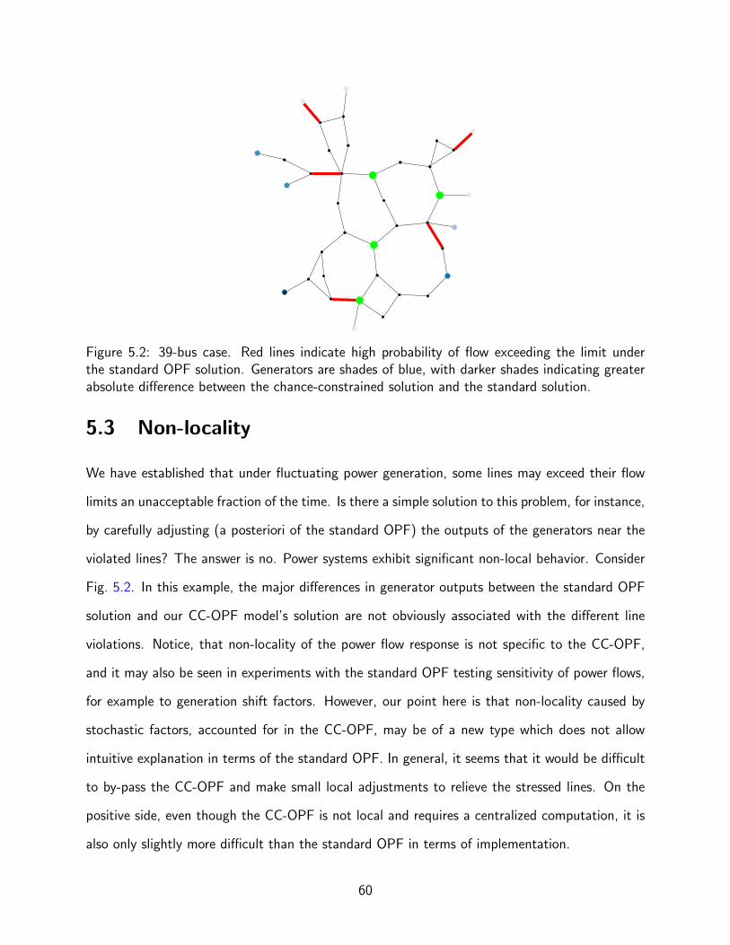
Figure 5.2: 39-bus case. Red lines indicate high probability of flow exceeding the limit underthe standard OPF solution. Generators are shades of blue, with darker shades indicating greaterabsolute difference between the chance-constrained solution and the standard solution.
5.3 Non-locality
We have established that under fluctuating power generation, some lines may exceed their flow
limits an unacceptable fraction of the time. Is there a simple solution to this problem, for instance,
by carefully adjusting (a posteriori of the standard OPF) the outputs of the generators near the
violated lines? The answer is no. Power systems exhibit significant non-local behavior. Consider
Fig. 5.2. In this example, the major differences in generator outputs between the standard OPF
solution and our CC-OPF model’s solution are not obviously associated with the different line
violations. Notice, that non-locality of the power flow response is not specific to the CC-OPF,
and it may also be seen in experiments with the standard OPF testing sensitivity of power flows,
for example to generation shift factors. However, our point here is that non-locality caused by
stochastic factors, accounted for in the CC-OPF, may be of a new type which does not allow
intuitive explanation in terms of the standard OPF. In general, it seems that it would be difficult
to by-pass the CC-OPF and make small local adjustments to relieve the stressed lines. On the
positive side, even though the CC-OPF is not local and requires a centralized computation, it is
also only slightly more difficult than the standard OPF in terms of implementation.
60
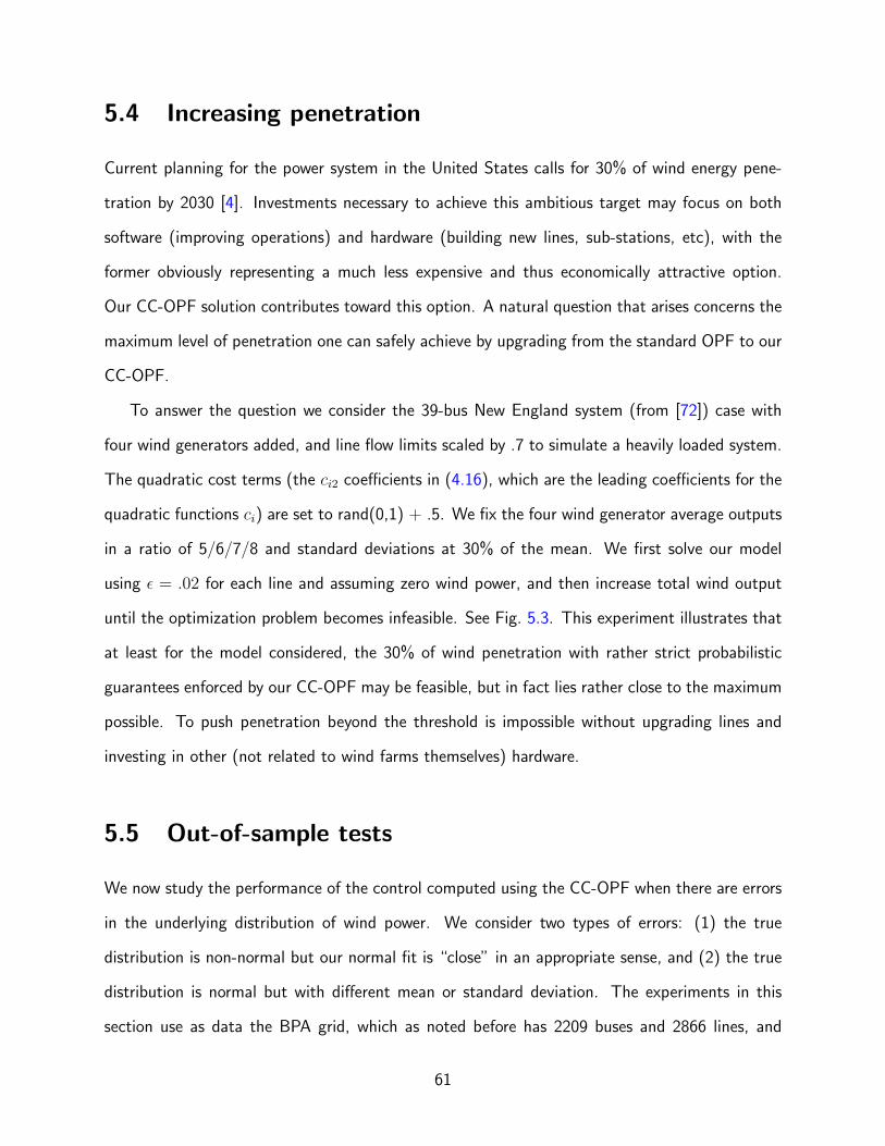
5.4 Increasing penetration
Current planning for the power system in the United States calls for 30% of wind energy pene-
tration by 2030 [4]. Investments necessary to achieve this ambitious target may focus on both
software (improving operations) and hardware (building new lines, sub-stations, etc), with the
former obviously representing a much less expensive and thus economically attractive option.
Our CC-OPF solution contributes toward this option. A natural question that arises concerns the
maximum level of penetration one can safely achieve by upgrading from the standard OPF to our
CC-OPF.
To answer the question we consider the 39-bus New England system (from [72]) case with
four wind generators added, and line flow limits scaled by .7 to simulate a heavily loaded system.
The quadratic cost terms (the ci2 coefficients in (4.16), which are the leading coefficients for the
quadratic functions ci) are set to rand(0,1) + .5. We fix the four wind generator average outputs
in a ratio of 5/6/7/8 and standard deviations at 30% of the mean. We first solve our model
using ε = .02 for each line and assuming zero wind power, and then increase total wind output
until the optimization problem becomes infeasible. See Fig. 5.3. This experiment illustrates that
at least for the model considered, the 30% of wind penetration with rather strict probabilistic
guarantees enforced by our CC-OPF may be feasible, but in fact lies rather close to the maximum
possible. To push penetration beyond the threshold is impossible without upgrading lines and
investing in other (not related to wind farms themselves) hardware.
5.5 Out-of-sample tests
We now study the performance of the control computed using the CC-OPF when there are errors
in the underlying distribution of wind power. We consider two types of errors: (1) the true
distribution is non-normal but our normal fit is “close” in an appropriate sense, and (2) the true
distribution is normal but with different mean or standard deviation. The experiments in this
section use as data the BPA grid, which as noted before has 2209 buses and 2866 lines, and
61
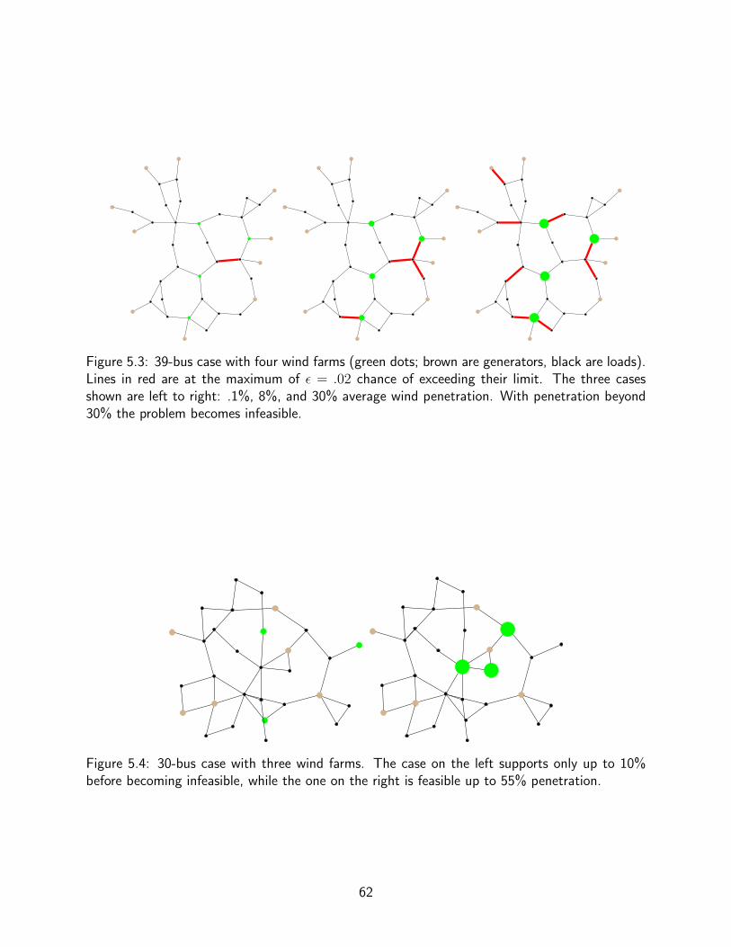
Figure 5.3: 39-bus case with four wind farms (green dots; brown are generators, black are loads).Lines in red are at the maximum of ε = .02 chance of exceeding their limit. The three casesshown are left to right: .1%, 8%, and 30% average wind penetration. With penetration beyond30% the problem becomes infeasible.
Figure 5.4: 30-bus case with three wind farms. The case on the left supports only up to 10%before becoming infeasible, while the one on the right is feasible up to 55% penetration.
62

collected wind data, altogether constituting a realistic test-case.
We first consider the non-normal case, using the following probability distributions, all with
fatter tails than tbe normal distrbution: (1) Laplace, (2) logistic, (3) Weibull (three different
shapes), (4) t location-scale with 2.5 degrees of freedom, and (5) Cauchy. For the Laplace
and logistic distributions, we simply match the mean and standard deviation. For the Weibull
distribution, we consider shape parameters k = 1.2, 2, 4 and choose the scale parameter to match
the standard deviations. We then translate to match means. For the t distribution, we fix 2.5
degrees of freedom and then choose the location and scale to match mean and standard deviation.
For the Cauchy distribution, we set the location parameter to the mean and choose the scale
parameter so as to match the 95th percentiles.
We use our model and solve under the normal distribution assumption, seeking a solution
which results in no line violations for cases within two standard deviations of the mean, i.e. a
maximum of about 2.27% chance of exceeding the limit. We then perform Monte Carlo tests
drawing from the above distributions to determine the actual rates of violation. See Fig. 5.5.
The worst-performer is the highly-asymmetric (and perhaps unreasonable) Weibull with shape
parameter 1.2, which approximately doubles the desired maximum chance of overload. Somewhat
surprisingly, the fat-tailed logistic and Student’s t distributions result in a maximum chance of
overload significantly less than desired, suggesting that our model is too conservative in these
cases.
Next we consider the normally distributed case with errors. We solve with nominal values for
the mean and standard deviation of wind power. We then consider the rate of violation after
scaling all means and standard deviations (separately). While the solution is sensitive to errors
in the mean forecast, the sensitivity is well-behaved. With a desired safety level of ε = 2.27%
for each line, an error in the mean of 25% results in a maximum 15% chance of exceeding the
limit. The solution is quite robust to errors in the standard deviation forecast, with a 25% error
resulting in less than 6% chance of overload. See Fig. 5.6.
63
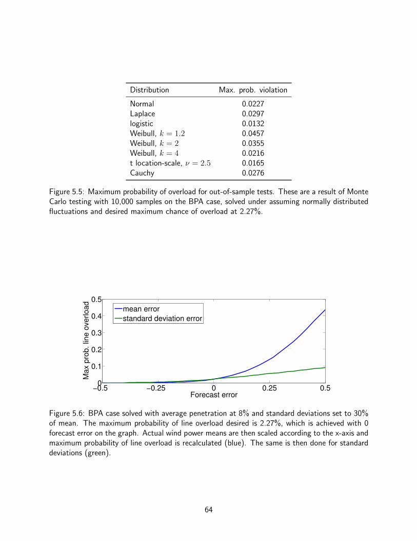
Distribution Max. prob. violation
Normal 0.0227Laplace 0.0297logistic 0.0132Weibull, k = 1.2 0.0457Weibull, k = 2 0.0355Weibull, k = 4 0.0216t location-scale, ν = 2.5 0.0165Cauchy 0.0276
Figure 5.5: Maximum probability of overload for out-of-sample tests. These are a result of MonteCarlo testing with 10,000 samples on the BPA case, solved under assuming normally distributedfluctuations and desired maximum chance of overload at 2.27%.
−0.5 −0.25 0 0.25 0.50
0.1
0.2
0.3
0.4
0.5
Forecast error
Max p
rob. lin
e o
verload
mean error
standard deviation error
Figure 5.6: BPA case solved with average penetration at 8% and standard deviations set to 30%of mean. The maximum probability of line overload desired is 2.27%, which is achieved with 0forecast error on the graph. Actual wind power means are then scaled according to the x-axis andmaximum probability of line overload is recalculated (blue). The same is then done for standarddeviations (green).
64
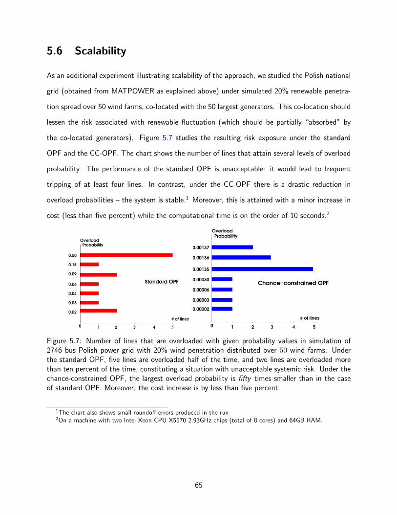
5.6 Scalability
As an additional experiment illustrating scalability of the approach, we studied the Polish national
grid (obtained from MATPOWER as explained above) under simulated 20% renewable penetra-
tion spread over 50 wind farms, co-located with the 50 largest generators. This co-location should
lessen the risk associated with renewable fluctuation (which should be partially “absorbed” by
the co-located generators). Figure 5.7 studies the resulting risk exposure under the standard
OPF and the CC-OPF. The chart shows the number of lines that attain several levels of overload
probability. The performance of the standard OPF is unacceptable: it would lead to frequent
tripping of at least four lines. In contrast, under the CC-OPF there is a drastic reduction in
overload probabilities – the system is stable.1 Moreover, this is attained with a minor increase in
cost (less than five percent) while the computational time is on the order of 10 seconds.2
1 2 3 40
ProbabilityOverload
Standard OPF
# of lines
5
0.50
0.09
0.15
0.06
0.04
0.03
0.02
1 3 40
ProbabilityOverload
# of lines
Chance−constrained OPF
2
0.00137
0.00136
0.00135
0.00003
0.00006
0.00002
5
0.00030
Figure 5.7: Number of lines that are overloaded with given probability values in simulation of2746 bus Polish power grid with 20% wind penetration distributed over 50 wind farms. Underthe standard OPF, five lines are overloaded half of the time, and two lines are overloaded morethan ten percent of the time, constituting a situation with unacceptable systemic risk. Under thechance-constrained OPF, the largest overload probability is fifty times smaller than in the caseof standard OPF. Moreover, the cost increase is by less than five percent.
1The chart also shows small roundoff errors produced in the run2On a machine with two Intel Xeon CPU X5570 2.93GHz chips (total of 8 cores) and 64GB RAM.
65

5.7 Changing locations for wind farms
In this example we consider the effect of changing locations of wind farms. We take the MAT-
POWER 30-bus case with line capacities scaled by .75 and add three wind farms with average
power output in a ratio of 2/3/4 and standard deviations at 30% of the average. Two choices
of locations are shown in Fig. 5.4. The first remains feasible for penetration up to 10% while the
second can withstand up to 55% penetration. This experiment shows that choosing location of
the wind farms is critical for achieving the ambitious goal of high renewable penetration.
5.8 Reversal of line flows
Here we consider the 9-bus case with two wind sources and 25% average penetration and standard
deviations set to 30% of the average case and analyze the following two somewhat rare but still
admissible wind configurations: (1) wind source (a) produces its average amount of power and
source (b) three standard deviations below average; (2) the reverse of the case (1). This results
in a substantial reversal of flow on a particular line shown in Fig. 5.8. This example suggests
that when evaluating and planning for grids with high-penetration of renewables one needs to be
aware of potentially fast and significant structural rearrangements of power flows. Flow reversals
and other qualitative changes of power flows, which are extremely rare in the grid of today, will
become significantly more frequent in the grid of tomorrow.
66
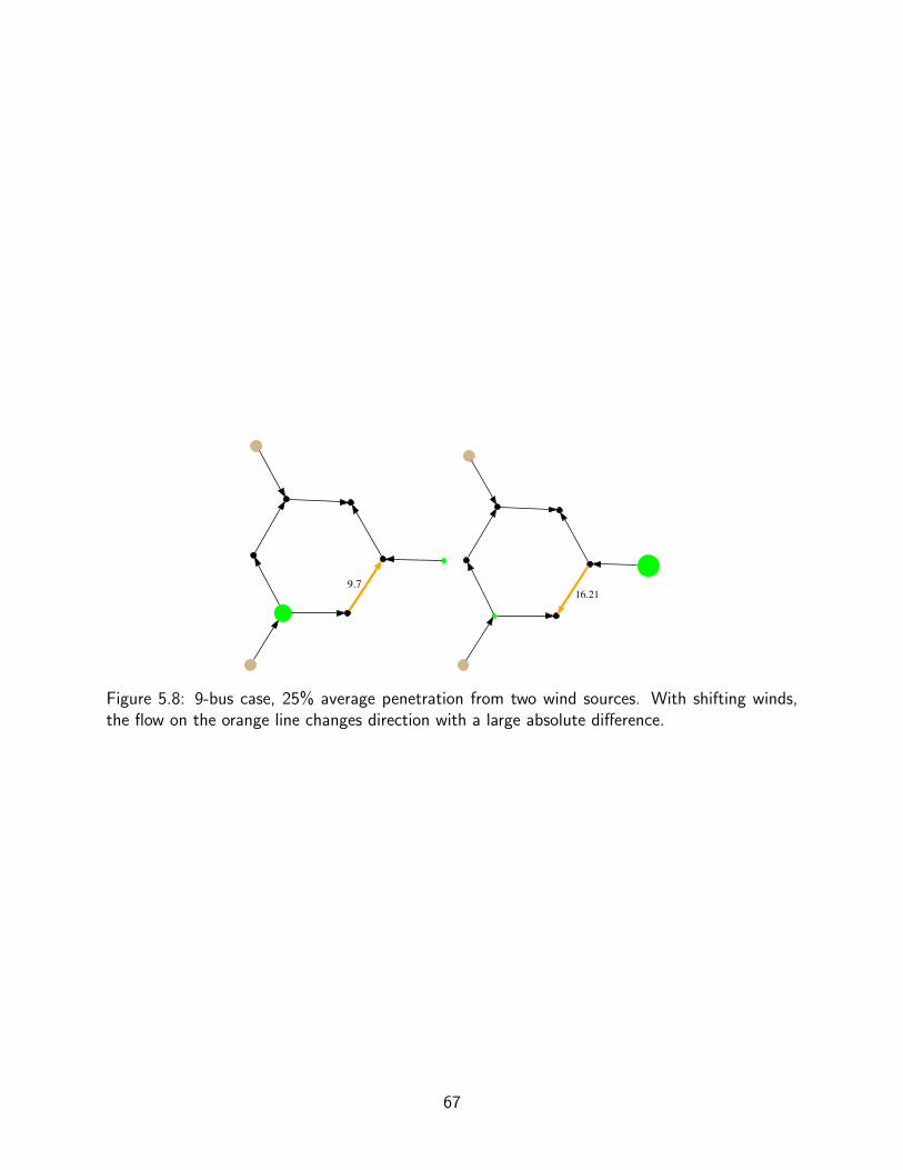
9.7
16.21
Figure 5.8: 9-bus case, 25% average penetration from two wind sources. With shifting winds,the flow on the orange line changes direction with a large absolute difference.
67
Part II
The power grid attack problem
68
Chapter 6
Introduction
6.1 Motivation
Large-scale blackouts of the power grid are massively disruptive to modern life. A serious black-
out can leave millions without power; shut down schools, offices, and hospitals; force essential
infrastructure like airports to rely on wasteful backup generators; and lead to economic losses
into the billions of dollars.
As we move toward a “smart” grid, we are at the same time encountering new stresses from
increased renewable generation, and growing threats from climate change and terrorism. More-
over, economic and environmental concerns have prevented the growth of power infrastructure to
keep pace with rising demand, so the grid operates ever closer to capacity [42]. Because of these
stresses on the modern power grid, the need to further understand the causes and properties of
blackouts has never been greater.
Modern power grids are usually quite robust to small disturbances, and are typically required
to operate under at least the “N - 1” criterion: the grid will continue to run safely after the failure
of a single element. After the failure, grid operators act quickly to restore the N-1 status so that
after a short period of time the grid can safely withstand an additional contingency. Thus, large
and expensive disruptions to the grid are usually caused by the failure of several components in
69
a small window of time.
This motivates a common topic in the study of power grid vulnerabilities, the so-called “N -
k problem” which asks: is there a set of k power lines whose simultaneous outage will result in
system failure? Rather than certifying the safety of the grid, in studying this problem one hopes
to identify potential weaknesses so that they might be addressed. It is an “agnostic” approach in
that it does not assume any particular structure for the attack – which is useful because failures
can come from a large number of sources (natural disasters, extreme weather events, physical
attack, human error, etc.) Of primary interest are small values of k; for large k (greater than 5
or so) there are usually a large number of damaging attacks, and for k = 1 simple enumeration
will work [20]. For large grids, combinatorial explosion makes the discrete problem intractable.
Furthermore, the equations that model the physical laws of power flows need to be solved in an
accurate and computationally practicable manner, which can be difficult for large grids.
6.1.1 Continuous formulation
One way to bypass this complexity is to consider a related continuous problem: instead of looking
at power line failures, let the impedances of the lines be increased. In the limit as resistance goes
to infinity, this is equivalent to removing the line. To simulate the idea of a small k, we impose
constraints on how much the impedances can be changed. The hope is that this modified problem
will have a combinatorial solution – the optimal attack will be to largely modify the impedance
of only a small number of lines, while perhaps slightly modifying many more lines. This way, the
solution to the continous problem also answers the original discrete question. In the numerical
experiments that follow we will see that this is indeed the case.
The next step is deciding what notion of “damage” to the grid we should consider. A number
of factors can lead to instability in the grid and the potential for a costly blackout, as discussed
in section 2.2. In [41] we investigate a variation of the problem discussed in this dissertation
that seeks to maximally disrupt voltage magnitudes; unlike line overages, which usually take
some time before causing the line to trip, voltage disturbances can lead to swift failures in the
70
grid, too fast for any mitigating action by a grid operator. Though the framework we developed
can accommodate both, the examples in this dissertation focus instead on maximally disrupting
voltage phase angle differences across lines. These are correlated with frequency instability and
a large angle difference can lead to loss of synchrony and sudden collapse of the grid.
Our formulation is then an optimization problem1:
An attacker seeks to maximally disrupt normal bus voltages by increasing the impedances of
power lines, constrained by a budget.
Note that after increasing the impedance on a number of lines, determining the voltage
disruption requires recomputing the power flows with the new grid configuration, which we achieve
with an OPF calculation. The approach can be described in terms of bilevel optimization: the
lower-level problem captures the disruption to the grid arising from a given set of attacked lines,
while the variables in the upper-level problem model the attack itself. Bilevel optimization can
be described as “mathematical programs with optimization problems in the constraints”; [28]
provides an overview of this sort of problem.
6.1.2 Is this realistic?
This attack model is unlikely to be encountered in practice exactly as described – it is doubtful
that a malicious agent would or could raise impedances on a particular set of power lines. But
it may still provide useful information about the vulnerability of the grid, as we will see in the
numerical experiments.
As an example, the model often times discovers attacks that create islands, which a combina-
torial formulation could be designed to find but may be too inefficient on large grids. Additionally,
the structure of the attacks discovered by the model mimicks that of grid conditions immediately
prior to historical blackouts: 1) a concentrated attack on a small number of lines and 2) a broad,
1We use the term “attacker” simply as a convenient way to describe the problem; we do not assume the gridwill actually be deliberately attacked. Our method is a vulnerability analysis which can help expose weaknessesto a large variety of events which may damage the grid, including but not limited to deliberate attack.
71
dispersed attack over a larger set of lines which can be interpreted as systemic stress that can
contribute significantly to the acute attack. So although the specific details of the attack mech-
anism may not be completely realistic, the model discovers sets of lines whose interdiction (even
in a partial sense) lead to disruption of the grid, which should be of interest to grid planners.
6.2 Attacker budget and the upper-level problem
To find interesting weaknesses in the grid, we impose a budget on the attacker’s ability to increase
impedances. By tuning the parameters of the budget we can find attacks of different strengths.
Setting the budget too low may result in an attack which has little effect on the grid. Too high a
budget on the other hand is likely to find a damaging attack, but it may be of little interest if it
involves extreme changes to a large number of lines – for instance, finding an attack of “disable
25% of all power lines” is unlikely to provide useful information to grid planners and operators.
The form of the budget we use is reminiscent of the “N-k” problem discussed in the intro-
duction to this section:
• the impedance of each line can be multiplied by a factor up to some γ
• the total amount of multiplication across all lines is bounded by κγ
In this, γ is a vector representing the increase in branch impedances in the following way: if
branch k has impedance zk, then under the attack its impedance is
z′k = (1 + γk)zk (6.1)
With this budget, the attacker can maximally attack κ lines. But unlike the “N-k” problem,
the attacker may choose to allocate his budget of κγ across many more than κ lines. This sort
of attack more closely resembles historical blackouts2 where only a small number of lines are
disabled, but many more lines are under various amounts of stress due to grid conditions.
2Such as the Northeast blackout of 2003 [2].
72

We can describe the two constraints with the following notation, from [41]:
eTγ ≤ κγ
0 ≤ γ ≤ γe
(6.2)
where e = (1, 1, ..., 1)T , the scalar γ is an upper bound for each line, and κ is the maximum
number of lines that can be attacked at the maximum level.
The upper-level problem is then to select a γ satisfying (6.2) which maximizes the appropriate
notion of voltage disruption. In [41] we chose to maximize the sum of squared differences in
voltage magnitude from 1.0 p.u.:
max∑k∈V
(|Vk| − 1)2
In this dissertation, I chose to focus mostly on maximizing the 1-norm of the vector of voltage
angle differences across branches:
F(γ) =∑
k,m∈L
|θk − θm| (6.3)
The choices of 1-norm versus 2-norm and angle versus magnitude cause the attacker to seek
different sorts of potential weaknesses in the power grid. The power flows on the grid change
after the attack via an optimal power flow computation, described in the next section. This is
what produces the voltage angles θk in Eq. (6.3).
6.3 Optimal power flow lower-level problem
After the grid is attacked, the line impedances are increased as in Eq. (6.1). We stated the
OPF (see section 2.6) in terms of admittances, however, and the equivalent adjustment for the
73

matrices G and B is3
Gkm(δ) =
Gkm
δkm + 1if k 6= m,
−∑l∈Ωk
Gkl(δ) if k = m.
(6.4)
Bkm(δ) =
Bkm
δkm + 1if k 6= m,
−∑l∈Ωk
Bkl(δ) if k = m.
(6.5)
Note that when γ = 0 the conductances and susceptances all retain their original values.
The power flow must change to account for this updated state of the grid while still satisfying
the power balance equations. We accomplish this by solving an OPF satisfying these conditions:
1. generator bus voltage magnitudes remain fixed
2. generator bus power injections and voltage angles vary
3. load bus power injections remained fixed
4. load bus voltage magnitudes and angles vary
5. line flow limits are not enforced
6. the sum of squared power injection changes at the generator buses is minimized
To clarify point 6: if generator bus g has power output P 0g + jQ0
g before the attack, the OPF
chooses Pg and Qg to minimize
H(P,Q, |V |, θ) =∑g∈G
(Pg − P 0g )2 + (Qg −Q0
g)2 (6.6)
where G is the set of generator buses. Note that generator bound constraints are not enforced;
the objective helps to keep generator outputs reasonable, but this is still a shortcoming that future
3As in the introduction to power flows in section 2.3, I have excluded the shunt terms here.
74
work should address. In the numerical experiments we found that strictly enforcing the generator
bounds lead to many more infeasible cases, indicating that load shedding or other measures would
be necessary and thus require a more complicated formulation. The OPF here is nonetheless an
improvement over our approach in [41], which used a simple power flow with a slack bus. With
that method, the slack bus could exhibit extremely erratic and unrealistic behavior when the grid
is attacked.
This OPF represents a somewhat realistic automatic response to the disturbance introduced
by γ: the generators adjust as little as possible to continue satisfying the demand at the load
buses. Unlike the classic power flow problem with a single slack bus, this OPF distributes the
change in power output across all the generators, which is a more reasonable approximation to
what happens in practice.
The complete formulation of the attack problem is then:
maxγ
∑k,m∈L
|θ∗k − θ∗m| s.t. (6.7a)
0 ≤ γkm ≤ γ ∀k,m ∈ E (6.7b)∑k,m∈L
γkm ≤ κγ (6.7c)
(P ∗, Q∗, |V |∗, θ∗) = argminP,Q,|V |,θ
∑g∈G
(Pg − P 0g )2 + (Qg −Q0
g)2 s.t (6.7d)
Pk = P 0k ∀k ∈ D (6.7e)
Qk = Q0k ∀k ∈ D (6.7f)
|Vk| = |Vk|0 ∀k ∈ G (6.7g)
Pk = |Vk|∑m∈K
|Vm|(Gkm(γ) cos θkm +Bkm(γ) sin θkm) ∀k ∈ V (6.7h)
Qk = |Vk|∑m∈K
|Vm|(Gkm(γ) sin θkm −Bkm(γ) cos θkm) ∀k ∈ V (6.7i)
δ is the attacker’s decision variable in the upper-level problem – the amount by which to
multiply the impedance of each line. Eq. (6.7a) is the upper-level (attacker’s) objective, to max-
75
imize the 1-norm of voltage angle differences. Constraints (6.7b)-(6.7c) represent the attacker’s
budget. Constraint (6.7d) states that the power flows will adjust according to the OPF in the
inner-level problem expressed in (6.7d)-(6.7i). Note that constraints (6.7h)-(6.7i) differ from
(2.22)-(2.23) in that the conductance and susceptance terms are now the γ-attacked versions
Gkm(δ) and Bkm(δ) from Eqs. (6.4)-(6.5). Also observe that line flow limits are not enforced –
this OPF does not include the constraints (2.20). Additionally, generator bound constraints are
not enforced.
6.4 Related work
The topic of vulnerability assessment for power grids is of great interest and considerable research
has been done on applying optimization methods to this problem. The papers [14,53,60] describe
a bilevel approach similar to ours, using binary decision variables so that a line is either fully
removed or not attacked at all, and focusing on loss of load as the attacker’s objective rather
than voltage disruption. The lower-level problem in the bilevel formulation is replaced by its dual
in [53] and is approximated using KKT conditions in [14].
By replacing the lower-level problem, these formulations have the disadvantage of allowing
spurious solutions of the power flow equations into the model, giving a misleading picture of the
effects of a prescribed attack on the grid. In this dissertation, we retain the bilevel structure,
solving the lower-level problem explicitly to more reliably rule out spurious solutions. A further
difference is that these papers use the linear DC approximation to describe the grid’s response to
an attack rather than the more accurate AC model used in this dissertation. Because a serious
attack can lead to extreme grid conditions in which the assumptions of the DC approximation do
not hold, we chose to use the more complicated full-AC model.
The paper [31] presents a bilevel formulation focusing on loss of load as the attack objective,
but with a lossless AC model. This is an improvement over the DC approximation, but it replaces
the lower-level problem with its KKT conditions as before. They use a continuous relaxation of
76
the binary decision variables comparable to ours. [57] pursues a similar strategy, but retains the
binary decision variables and approximates the single-level problem with a purely combinatorial
reduction of the problem that bypasses direct solution of the nonlinear AC equations.
The paper [33] explores a problem closely related to ours, examining heavily congested trans-
mission grids with infeasible configurations of generation and load. The source of the congestion
is either high load or a problematic injection of uncontrollable fluctuating generation4 combined
with the automatic response of controllable generation. The authors explore the problem of re-
lieving this congestion by installing a minimal set of Flexible Alternating Current Transmission
System devices, which modify the reactance of the transmission lines. They use a sequential
linearization method to solve the resulting bilevel optimization problem.
In [20], the problem is stated most closely to our formulation, but it uses the DC approxi-
mation: a fictitious attacker modifies reactances (rather than impedances as in the AC model)
to maximally overload any power line. Because power flow on a line is a simple function of the
branch angle difference in the DC model, this objective is closely related to ours.
4Note the similarity to part I.
77
Chapter 7
Solving the attack problem
We now describe our procedure for solving the attack problem as formulated in the previous
section. To recap: we are looking for a set of impedance multipliers, constrained by a budget, that
will cause maximum disruption to normal grid voltages. We formulate this as a bilevel optimization
problem, where in the upper-level problem (section 6.2) an attacker selects impedance multipliers
within his budget, and in the lower-level problem (section 6.3) the grid responds via an optimal
power flow problem which minimizes changes in power output at the generators.
We use MATPOWER [72] to solve the OPF lower-level problem. To solve the upper-level
problem, we use the Frank-Wolfe algorithm [32] for constrained optimization, which we describe
in section 7.3. The problem is non-convex, so the Frank-Wolfe algorithm is not guaranteed to
converge to a global optimum; we sometimes use multiple random restarts to help find a good
local optimum. Our objective does not allow for a convenient analytic form for the gradient,
so we use a finite-difference approximation. This is expensive on large grids, so we investigated
some derivative-free approaches. We also explored a branching approach to help avoid inferior
local optima and to find many different near-optimal attacks.
78
7.1 Solving the OPF lower-level problem
A primary tool in all of these analyses is MATPOWER [72], a package of MATLAB files for
solving power flow problems. With MATPOWER, it is possible to use a number of internal and
third-party solvers. We used the IPOPT [66] with PARDISO solver [11,61,62], which we observed
to perform best after much experimentation. In certain cases where the OPF failed to converge,
we checked with the semidefinite program solver [51] to confirm infeasibility.
7.2 Non-convexity and multiple local optima
The lower-level OPF subproblem is itself nonconvex and in practice may have many local solutions,
as discussed in section 2.6.1. Wrapping this with an additional optimization problem does not
help the issue. Standard gradient-based optimization methods (such as the Frank-Wolfe algorithm
described in the next section) are thus not guaranteed to find a global optimum. We use random
restarts to find a good local optimum, though this provides no guarantees either.
Fig. 7.1 provides a simple example of the problem. In this example, we attack two differ-
ent lines in the 5-bus grid “case5” from MATPOWER. The objective is the 1-norm of voltage
magnitude differences from 1.0 p.u.:∑
k∈V ||Vk| − 1|. The attack is constrained to a maximum
multiplier of γ + 1 = 3.5 and restricted so that only lines 2, 3 and 3, 4 can be attacked.
The left image shows the objective for all attacks on the two lines with γ values in the region
[0, 2.5] × [0, 2.5], so that κ = 2 (two lines can be maximally attacked). The global optimum in
this case is at (2.5, 2.5), but there is a local optimum at (0.66, 0). Furthermore, and not shown
in the figure, there is actually a local optimum at the origin, so that starting from zero results in
a very weak attack.
If we set κ = 1, we are restricted to the region to the left and below the dotted line. In
this case the global optimum is (0.66, 0) but there is a local optimum at (2.5, 0). If we further
restrict the attack to use all of the budget, so that γ23 + γ34 = κγ, then the feasible region is
the dotted line. In this case the global optimum is at (.46, 2.04) and again (2.5, 0) is a local
79
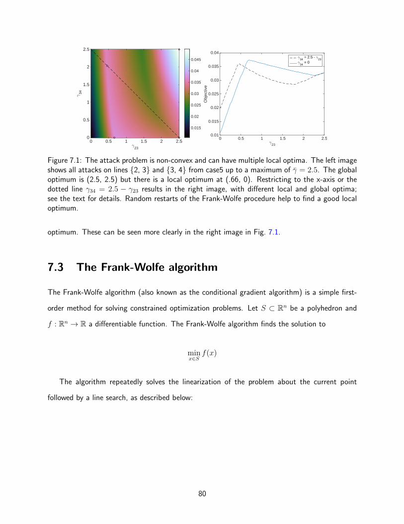
.23
0 0.5 1 1.5 2 2.5
.34
0
0.5
1
1.5
2
2.5
0.015
0.02
0.025
0.03
0.035
0.04
0.045
.23
0 0.5 1 1.5 2 2.5
Obj
ectiv
e
0.01
0.015
0.02
0.025
0.03
0.035
0.04.
34 = 2.5 - .
23.
34 = 0
Figure 7.1: The attack problem is non-convex and can have multiple local optima. The left imageshows all attacks on lines 2, 3 and 3, 4 from case5 up to a maximum of γ = 2.5. The globaloptimum is (2.5, 2.5) but there is a local optimum at (.66, 0). Restricting to the x-axis or thedotted line γ34 = 2.5 − γ23 results in the right image, with different local and global optima;see the text for details. Random restarts of the Frank-Wolfe procedure help to find a good localoptimum.
optimum. These can be seen more clearly in the right image in Fig. 7.1.
7.3 The Frank-Wolfe algorithm
The Frank-Wolfe algorithm (also known as the conditional gradient algorithm) is a simple first-
order method for solving constrained optimization problems. Let S ⊂ Rn be a polyhedron and
f : Rn → R a differentiable function. The Frank-Wolfe algorithm finds the solution to
minx∈S
f(x)
The algorithm repeatedly solves the linearization of the problem about the current point
followed by a line search, as described below:
80
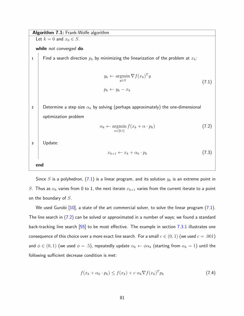
Algorithm 7.1: Frank-Wolfe algorithm
Let k = 0 and x0 ∈ S.
while not converged do
1 Find a search direction pk by minimizing the linearization of the problem at xk:
yk ← argminy∈S
∇f(xk)Ty
pk ← yk − xk(7.1)
2 Determine a step size αk by solving (perhaps approximately) the one-dimensional
optimization problem
αk ← argminα∈[0,1]
f(xk + α · pk) (7.2)
3 Update:
xk+1 ← xk + αk · pk (7.3)
end
Since S is a polyhedron, (7.1) is a linear program, and its solution yk is an extreme point in
S. Thus as αk varies from 0 to 1, the next iterate xk+1 varies from the current iterate to a point
on the boundary of S.
We used Gurobi [10], a state of the art commercial solver, to solve the linear program (7.1).
The line search in (7.2) can be solved or approximated in a number of ways; we found a standard
back-tracking line search [55] to be most effective. The example in section 7.3.1 illustrates one
consequence of this choice over a more exact line search. For a small c ∈ (0, 1) (we used c = .001)
and φ ∈ (0, 1) (we used φ = .5), repeatedly update αk ← φαk (starting from αk = 1) until the
following sufficient decrease condition is met:
f(xk + αk · pk) ≤ f(xk) + c αk∇f(xk)Tpk (7.4)
81

For our problem, the line search typically finds a suitable step size in fewer than ten function
evaluations. Especially for large grids, this is much smaller than the number of evaluations
required in the finite-difference approximation to the gradient, that is to say the run-time of the
line-search has little impact on the overall runtime of the algorithm.
Steps 1-3 repeat until one of the following three conditions holds:
1. improvement between iterations in the objective is less than some tolerance
2. the step size in the line search is less than some tolerance
3. the number of iterations exceeds some maximum
The third condition is a practical safeguard and we do not count it as successful convergence.
Under appropriate conditions the Frank-Wolfe algorithm is guaranteed to converge to the optimal
solution [24, 38], though sublinearly: convergence requires at most O(1ε) steps to get within ε
of the optimal value. This is typical of first-order methods – optimization methods that use
only first-derivative information without taking curvature into account. As described previously,
however, our problem is not well-behaved and the method does not enjoy these guarantees. But
in the examples we will see that it often finds good solutions.
Though they require more iterations to converge than more sophisticated techniques, Frank-
Wolfe and similar first-order methods are used widely and successfully in many fields, especially
machine learning [39]. There are several reasons for this, including:
• First-order methods often have very low complexity per iteration
• In many applications, moderately accurate solutions are sufficient and can be found more
quickly with a simple method
• Data is often corrupted or only known approximately, and uncertain data does not justify
the precise solutions of a sophisticated method
82
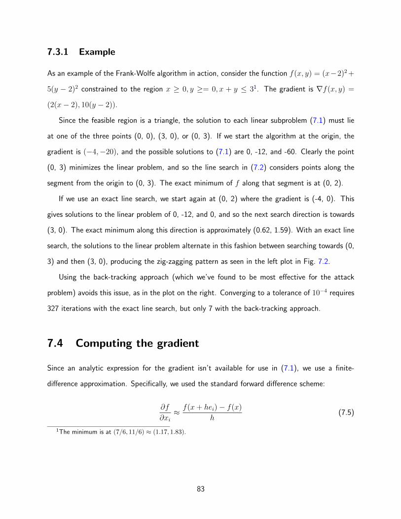
7.3.1 Example
As an example of the Frank-Wolfe algorithm in action, consider the function f(x, y) = (x−2)2 +
5(y − 2)2 constrained to the region x ≥ 0, y ≥= 0, x + y ≤ 31. The gradient is ∇f(x, y) =
(2(x− 2), 10(y − 2)).
Since the feasible region is a triangle, the solution to each linear subproblem (7.1) must lie
at one of the three points (0, 0), (3, 0), or (0, 3). If we start the algorithm at the origin, the
gradient is (−4,−20), and the possible solutions to (7.1) are 0, -12, and -60. Clearly the point
(0, 3) minimizes the linear problem, and so the line search in (7.2) considers points along the
segment from the origin to (0, 3). The exact minimum of f along that segment is at (0, 2).
If we use an exact line search, we start again at (0, 2) where the gradient is (-4, 0). This
gives solutions to the linear problem of 0, -12, and 0, and so the next search direction is towards
(3, 0). The exact minimum along this direction is approximately (0.62, 1.59). With an exact line
search, the solutions to the linear problem alternate in this fashion between searching towards (0,
3) and then (3, 0), producing the zig-zagging pattern as seen in the left plot in Fig. 7.2.
Using the back-tracking approach (which we’ve found to be most effective for the attack
problem) avoids this issue, as in the plot on the right. Converging to a tolerance of 10−4 requires
327 iterations with the exact line search, but only 7 with the back-tracking approach.
7.4 Computing the gradient
Since an analytic expression for the gradient isn’t available for use in (7.1), we use a finite-
difference approximation. Specifically, we used the standard forward difference scheme:
∂f
∂xi≈ f(x+ hei)− f(x)
h(7.5)
1The minimum is at (7/6, 11/6) ≈ (1.17, 1.83).
83
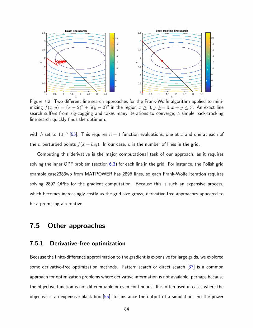
Exact line search
x0 0.5 1 1.5 2 2.5 3 3.5
y
0
0.5
1
1.5
2
2.5
3
3.5
4
6
8
10
12
14
16
18
20
Back-tracking line search
x0 0.5 1 1.5 2 2.5 3 3.5
y
0
0.5
1
1.5
2
2.5
3
3.5
4
6
8
10
12
14
16
18
20
Figure 7.2: Two different line search approaches for the Frank-Wolfe algorithm applied to mini-mizing f(x, y) = (x − 2)2 + 5(y − 2)2 in the region x ≥ 0, y ≥= 0, x + y ≤ 3. An exact linesearch suffers from zig-zagging and takes many iterations to converge; a simple back-trackingline search quickly finds the optimum.
with h set to 10−8 [55]. This requires n + 1 function evaluations, one at x and one at each of
the n perturbed points f(x+ hei). In our case, n is the number of lines in the grid.
Computing this derivative is the major computational task of our approach, as it requires
solving the inner OPF problem (section 6.3) for each line in the grid. For instance, the Polish grid
example case2383wp from MATPOWER has 2896 lines, so each Frank-Wolfe iteration requires
solving 2897 OPFs for the gradient computation. Because this is such an expensive process,
which becomes increasingly costly as the grid size grows, derivative-free approaches appeared to
be a promising alternative.
7.5 Other approaches
7.5.1 Derivative-free optimization
Because the finite-difference approximation to the gradient is expensive for large grids, we explored
some derivative-free optimization methods. Pattern search or direct search [37] is a common
approach for optimization problems where derivative information is not available, perhaps because
the objective function is not differentiable or even continuous. It is often used in cases where the
objective is an expensive black box [55], for instance the output of a simulation. So the power
84
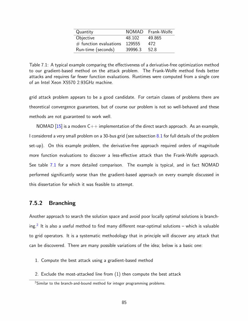
Quantity NOMAD Frank-WolfeObjective 48.102 49.865# function evaluations 129555 472Run-time (seconds) 39996.3 52.8
Table 7.1: A typical example comparing the effectiveness of a derivative-free optimization methodto our gradient-based method on the attack problem. The Frank-Wolfe method finds betterattacks and requires far fewer function evaluations. Runtimes were computed from a single coreof an Intel Xeon X5570 2.93GHz machine.
grid attack problem appears to be a good candidate. For certain classes of problems there are
theoretical convergence guarantees, but of course our problem is not so well-behaved and these
methods are not guaranteed to work well.
NOMAD [15] is a modern C++ implementation of the direct search approach. As an example,
I considered a very small problem on a 30-bus grid (see subsection 8.1 for full details of the problem
set-up). On this example problem, the derivative-free approach required orders of magnitude
more function evaluations to discover a less-effective attack than the Frank-Wolfe approach.
See table 7.1 for a more detailed comparison. The example is typical, and in fact NOMAD
performed significantly worse than the gradient-based approach on every example discussed in
this dissertation for which it was feasible to attempt.
7.5.2 Branching
Another approach to search the solution space and avoid poor locally optimal solutions is branch-
ing.2 It is also a useful method to find many different near-optimal solutions – which is valuable
to grid operators. It is a systematic methodology that in principle will discover any attack that
can be discovered. There are many possible variations of the idea; below is a basic one:
1. Compute the best attack using a gradient-based method
2. Exclude the most-attacked line from (1) then compute the best attack
2Similar to the branch-and-bound method for integer programming problems.
85

3. Exclude the most-attacked line from (1) and ‘force-include’ the second most-attacked line,
then compute the best attack
4. Exclude the second most-attacked line from (1) and ‘force-include’ the most-attacked line,
then compute the best attack
5. Exclude the second most-attacked line from (1) then compute the best attack
6. ...
A concrete example of the technique on the 57-bus case is described in subsection 8.2. In
that example, branching finds a more damaging attack than the Frank-Wolfe procedure alone,
which converges to a less effective local optimum.
86

Chapter 8
Numerical experiments
In this chapter we investigate the properties of the attacks discovered by our model in a number
of numerical experiments. We will begin by examining a small grid where it is easy to visualize
the changes forced upon the grid by the attack. We will also look at much larger actual-scale
grids, which are more difficult to visualize but we can still see that the model discovers damaging
attacks. Additionally, we will consider an example of the branching procedure described in section
7.5.2 which can sometimes find more effective attacks by avoiding local optima.
8.1 9-bus example
To illustrate the nature of this attack problem, we examine a small example grid. For a small case,
we can easily visualize the effect of various attacks on the grid. We can also quickly compute the
result for all(nk
)attacks which allocate the entire budget across k of the grid’s n lines. We will
see that our procedure finds the best of these very quickly. We will also see that the impact on
the grid varies widely between different attacks of the same strength.
In this example we will look at “case9” (Fig. 8.1) from MATPOWER which has nine buses
– three generators, three load buses with positive demand, three buses with zero demand – and
nine branches.
87

1
4
2
3
6
57
8
9
Figure 8.1: case9 from MATPOWER, rendered by graphviz [34]. Generator buses are in green,load buses are in black. Buses with neither demand nor generation are grey.
objective type voltage angleobjective norm L1
γ 2.5κ 3
Table 8.1: Attack problem parameters for case9 example
8.1.1 Attack parameters
Let the attacker’s objective be to maximize the 1-norm of phase angle differences. We set the
attacker’s budget to γ = 2.5 and κ = 3, i.e. he can multiply the impedance of a particular line
by up to γ + 1 = 3.5 and he can maximally attack up to κ = 3 lines.
8.1.2 Results
Our procedure quickly converges to allocating the entire attack budget on only three lines.1 This
sort of result is not typical; the optical attack usually spreads the budget over many more than
κ lines. But in this case it allows us to consider all of the(
93
)= 84 attacks which fully allocate
the budget to three lines, and see how our proposed attack compares.
1From a zero start and most random starts, it converges to this solution in two iterations
88
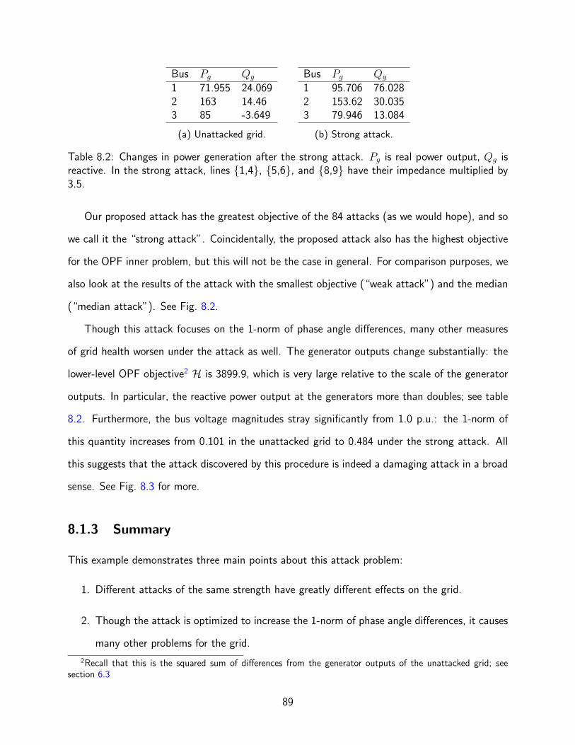
Bus Pg Qg
1 71.955 24.0692 163 14.463 85 -3.649
(a) Unattacked grid.
Bus Pg Qg
1 95.706 76.0282 153.62 30.0353 79.946 13.084
(b) Strong attack.
Table 8.2: Changes in power generation after the strong attack. Pg is real power output, Qg isreactive. In the strong attack, lines 1,4, 5,6, and 8,9 have their impedance multiplied by3.5.
Our proposed attack has the greatest objective of the 84 attacks (as we would hope), and so
we call it the “strong attack”. Coincidentally, the proposed attack also has the highest objective
for the OPF inner problem, but this will not be the case in general. For comparison purposes, we
also look at the results of the attack with the smallest objective (“weak attack”) and the median
(“median attack”). See Fig. 8.2.
Though this attack focuses on the 1-norm of phase angle differences, many other measures
of grid health worsen under the attack as well. The generator outputs change substantially: the
lower-level OPF objective2 H is 3899.9, which is very large relative to the scale of the generator
outputs. In particular, the reactive power output at the generators more than doubles; see table
8.2. Furthermore, the bus voltage magnitudes stray significantly from 1.0 p.u.: the 1-norm of
this quantity increases from 0.101 in the unattacked grid to 0.484 under the strong attack. All
this suggests that the attack discovered by this procedure is indeed a damaging attack in a broad
sense. See Fig. 8.3 for more.
8.1.3 Summary
This example demonstrates three main points about this attack problem:
1. Different attacks of the same strength have greatly different effects on the grid.
2. Though the attack is optimized to increase the 1-norm of phase angle differences, it causes
many other problems for the grid.
2Recall that this is the squared sum of differences from the generator outputs of the unattacked grid; seesection 6.3
89
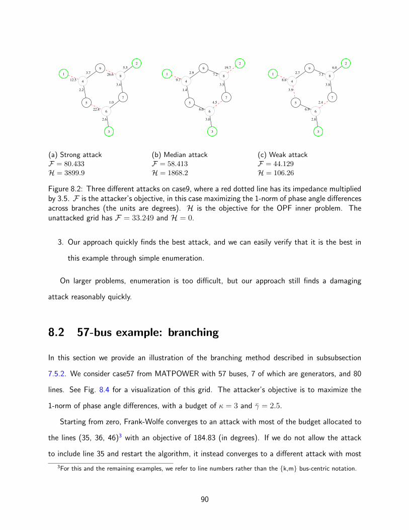
1
4 12.5
2
3
6
2.6
5
2.2
7 1.0
8
5.5 9 26.6
22.8
3.4
3.7
(a) Strong attackF = 80.433H = 3899.9
1
4 9.7
2
3
6
3.0
5
1.4
7 4.5
8
19.7 9 7.2
6.6
3.5
2.9
(b) Median attackF = 58.413H = 1868.2
1
4 8.6
2
3
6
2.8
5
3.9
7 2.4
8
6.0 9 7.1
6.9
3.8
2.7
(c) Weak attackF = 44.129H = 106.26
Figure 8.2: Three different attacks on case9, where a red dotted line has its impedance multipliedby 3.5. F is the attacker’s objective, in this case maximizing the 1-norm of phase angle differencesacross branches (the units are degrees). H is the objective for the OPF inner problem. Theunattacked grid has F = 33.249 and H = 0.
3. Our approach quickly finds the best attack, and we can easily verify that it is the best in
this example through simple enumeration.
On larger problems, enumeration is too difficult, but our approach still finds a damaging
attack reasonably quickly.
8.2 57-bus example: branching
In this section we provide an illustration of the branching method described in subsubsection
7.5.2. We consider case57 from MATPOWER with 57 buses, 7 of which are generators, and 80
lines. See Fig. 8.4 for a visualization of this grid. The attacker’s objective is to maximize the
1-norm of phase angle differences, with a budget of κ = 3 and γ = 2.5.
Starting from zero, Frank-Wolfe converges to an attack with most of the budget allocated to
the lines (35, 36, 46)3 with an objective of 184.83 (in degrees). If we do not allow the attack
to include line 35 and restart the algorithm, it instead converges to a different attack with most
3For this and the remaining examples, we refer to line numbers rather than the k,m bus-centric notation.
90
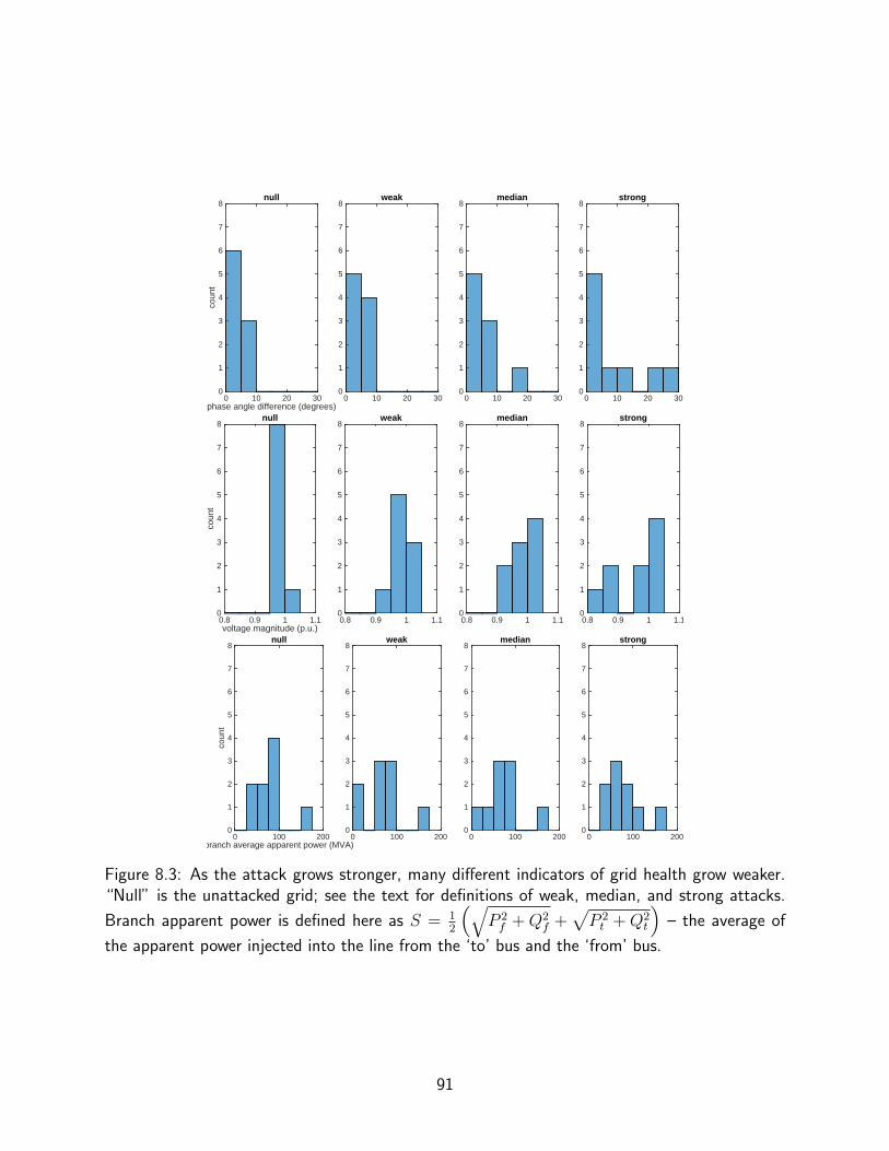
phase angle difference (degrees)0 10 20 30
coun
t
0
1
2
3
4
5
6
7
8null
0 10 20 300
1
2
3
4
5
6
7
8weak
0 10 20 300
1
2
3
4
5
6
7
8median
0 10 20 300
1
2
3
4
5
6
7
8strong
voltage magnitude (p.u.)0.8 0.9 1 1.1
coun
t
0
1
2
3
4
5
6
7
8null
0.8 0.9 1 1.10
1
2
3
4
5
6
7
8weak
0.8 0.9 1 1.10
1
2
3
4
5
6
7
8median
0.8 0.9 1 1.10
1
2
3
4
5
6
7
8strong
branch average apparent power (MVA)0 100 200
coun
t
0
1
2
3
4
5
6
7
8null
0 100 2000
1
2
3
4
5
6
7
8weak
0 100 2000
1
2
3
4
5
6
7
8median
0 100 2000
1
2
3
4
5
6
7
8strong
Figure 8.3: As the attack grows stronger, many different indicators of grid health grow weaker.“Null” is the unattacked grid; see the text for definitions of weak, median, and strong attacks.
Branch apparent power is defined here as S = 12
(√P 2f +Q2
f +√P 2t +Q2
t
)– the average of
the apparent power injected into the line from the ‘to’ bus and the ‘from’ bus.
91
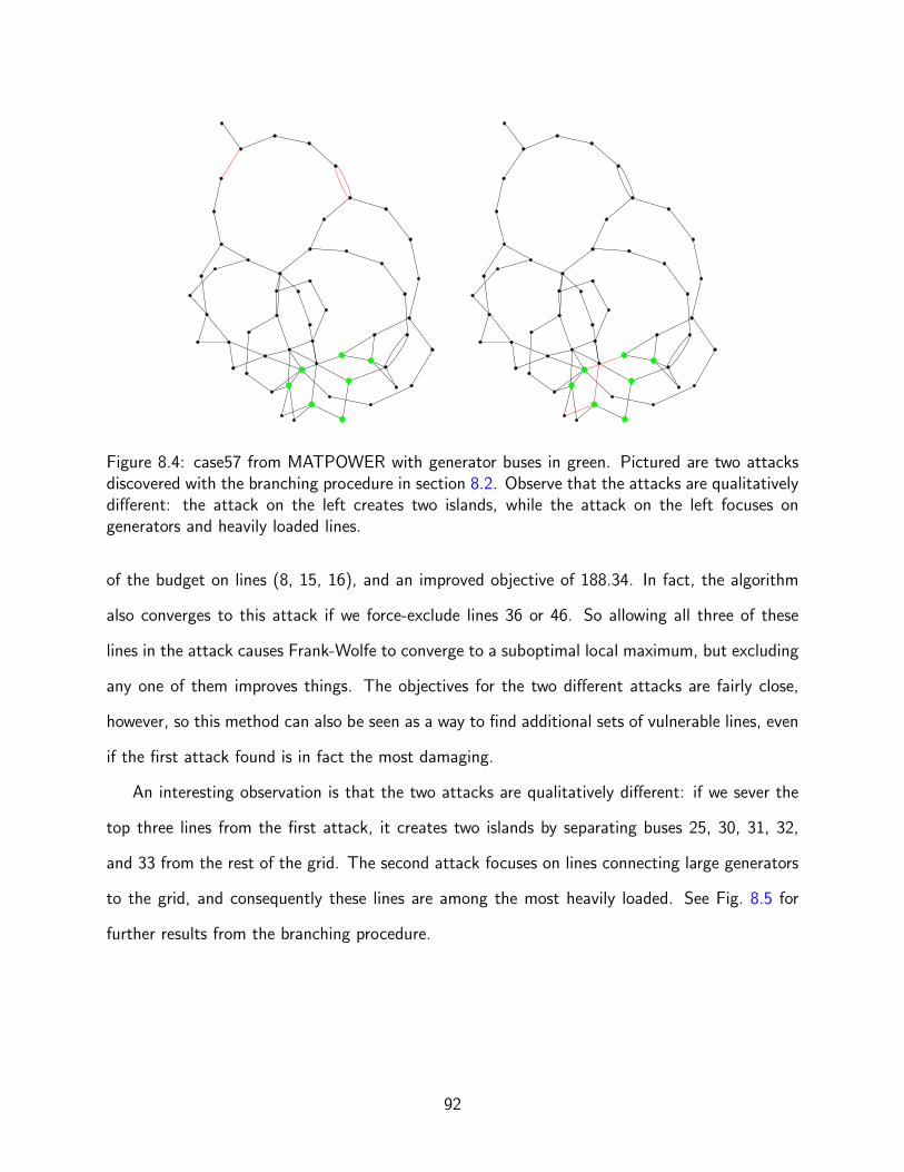
Figure 8.4: case57 from MATPOWER with generator buses in green. Pictured are two attacksdiscovered with the branching procedure in section 8.2. Observe that the attacks are qualitativelydifferent: the attack on the left creates two islands, while the attack on the left focuses ongenerators and heavily loaded lines.
of the budget on lines (8, 15, 16), and an improved objective of 188.34. In fact, the algorithm
also converges to this attack if we force-exclude lines 36 or 46. So allowing all three of these
lines in the attack causes Frank-Wolfe to converge to a suboptimal local maximum, but excluding
any one of them improves things. The objectives for the two different attacks are fairly close,
however, so this method can also be seen as a way to find additional sets of vulnerable lines, even
if the first attack found is in fact the most damaging.
An interesting observation is that the two attacks are qualitatively different: if we sever the
top three lines from the first attack, it creates two islands by separating buses 25, 30, 31, 32,
and 33 from the rest of the grid. The second attack focuses on lines connecting large generators
to the grid, and consequently these lines are among the most heavily loaded. See Fig. 8.5 for
further results from the branching procedure.
92
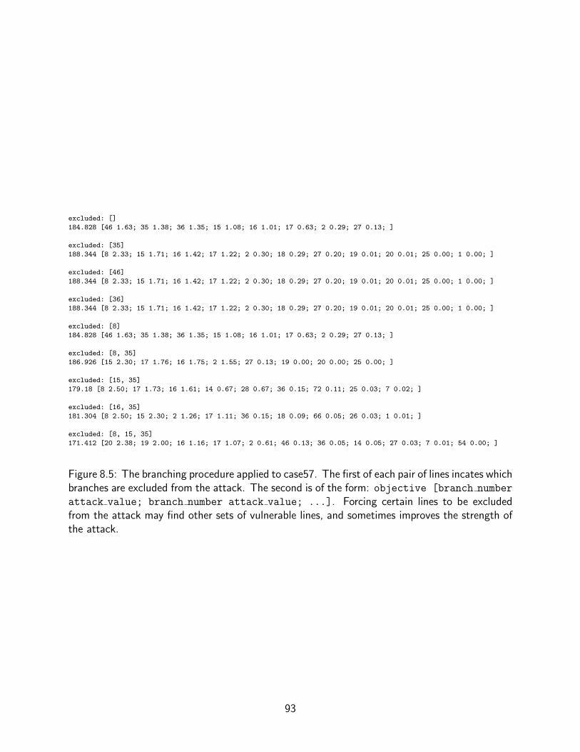
excluded: []
184.828 [46 1.63; 35 1.38; 36 1.35; 15 1.08; 16 1.01; 17 0.63; 2 0.29; 27 0.13; ]
excluded: [35]
188.344 [8 2.33; 15 1.71; 16 1.42; 17 1.22; 2 0.30; 18 0.29; 27 0.20; 19 0.01; 20 0.01; 25 0.00; 1 0.00; ]
excluded: [46]
188.344 [8 2.33; 15 1.71; 16 1.42; 17 1.22; 2 0.30; 18 0.29; 27 0.20; 19 0.01; 20 0.01; 25 0.00; 1 0.00; ]
excluded: [36]
188.344 [8 2.33; 15 1.71; 16 1.42; 17 1.22; 2 0.30; 18 0.29; 27 0.20; 19 0.01; 20 0.01; 25 0.00; 1 0.00; ]
excluded: [8]
184.828 [46 1.63; 35 1.38; 36 1.35; 15 1.08; 16 1.01; 17 0.63; 2 0.29; 27 0.13; ]
excluded: [8, 35]
186.926 [15 2.30; 17 1.76; 16 1.75; 2 1.55; 27 0.13; 19 0.00; 20 0.00; 25 0.00; ]
excluded: [15, 35]
179.18 [8 2.50; 17 1.73; 16 1.61; 14 0.67; 28 0.67; 36 0.15; 72 0.11; 25 0.03; 7 0.02; ]
excluded: [16, 35]
181.304 [8 2.50; 15 2.30; 2 1.26; 17 1.11; 36 0.15; 18 0.09; 66 0.05; 26 0.03; 1 0.01; ]
excluded: [8, 15, 35]
171.412 [20 2.38; 19 2.00; 16 1.16; 17 1.07; 2 0.61; 46 0.13; 36 0.05; 14 0.05; 27 0.03; 7 0.01; 54 0.00; ]
Figure 8.5: The branching procedure applied to case57. The first of each pair of lines incates whichbranches are excluded from the attack. The second is of the form: objective [branch number
attack value; branch number attack value; ...]. Forcing certain lines to be excludedfrom the attack may find other sets of vulnerable lines, and sometimes improves the strength ofthe attack.
93

Attack ObjectiveFrank-Wolfe 625Head 612Simple 596Tail 471None 464
Table 8.3: Objective values for different attacks on case118. See the text for the definitions ofthe different attacks.
8.3 118-bus example: head and tail
This example is much larger, but still small enough to visualize. The IEEE 118-bus test case
(included in MATPOWER, see Fig. 8.7) has 54 generators and 186 branches. Considering all
attacks of three lines at maximal strength is(
1863
)≈ 106 attacks.
But this time, as is typically the case, the optimal attack with parameters as in table 8.1
spreads the budget over many more than three lines. The majority of the budget is allocated to
a small number of lines, but the remainder is spread thinly over a larger number of lines, though
still a small fraction of the total number of lines in the grid. This sort of attack mimicks what
has been observed in actual historical blackouts: a handful of lines are taken out, but a much
larger number are stressed due to grid conditions.
We examine the relative impact of these two pieces of the attack – the strong attack on a few
lines and the general “malaise” over many more lines. A typical random start of the Frank-Wolfe
approach progresses as in Fig. 8.8. Notably, the majority of the budget is allocated between the
six lines (38 96 31 33 67 66), the “head” of the attack. The rest of the budget is spread over
a few dozen more lines, the “tail”. The unattacked grid has an objective value of 464. The
Frank-Wolfe attack achieves an objective of 625. Attacking only the head and setting to zero
the attack on the tail gives an objective of 612. After enumerating all possible attacks of κ = 3
at maximal strength γ = 5.0, the best result is (9 38 96) with an objective of 596. Setting the
attack to zero on the head and only considering the tail gives and objective of 471. See table 8.3
for a summary and Fig. 8.6 for histograms of the phase angle differences under each attack.
94

Figure 8.6: Histogram of phase angle differences under different attacks on case118. Notice thatthe Frank-Wolfe attack increases the phase angle difference on many branches to over 20 degrees.
This result is typical: the majority of the impact of the attack comes from hitting a few
lines hard, but the weaker tail of the attack contributes significantly as well, producing a more
damaging attack than focusing entirely on a few lines.
8.4 Large-scale example on the Polish grid
Our approach scales up to realistic, national-scale power grids. MATPOWER includes data for a
number of configurations of the Polish power grid. I ran the algorithm on the 2383-bus winter
1999-2000 peak data “case2383wp.m” with 327 generators and 2896 branches.
The individual inner OPF problems are relatively expensive for problems of this size, taking up
to a second to solve on a machine with two Intel Xeon CPU X5570 2.93GHz chips (total of 8 cores)
and 64GB RAM. Since grids this big require solving thousands of these OPFs for each gradient,
it is worthwhile to parallelize this computation. Computing the gradient is embarrassingly parallel
and can be accomplished in MATLAB with a simple parfor loop to take advantage of all available
cores.
With a budget of (κ = 5, γ = 5.0) and objective to maximize the 1-norm of angle differences,
95
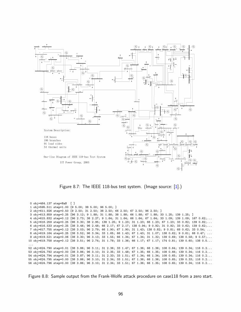
1 2
4
5
6 7
8
9
10
11
12
13
14
117
15
16
17
18
19
20
21
22
23
25
26
27
28
29
113 30
31
32
114115
33
34
35
36
37
38
39
40 41 42
43
44
45
4746
48
49
50
51
52
53 54 5556
5758
59
60
61
62
63
64
65
66
67
68
116
69
70
71
72
73
24
74
75
118 76
77
78
79
80
81
82
8384
85
86
87
88 89
9091
92
93
9495
96
97
98
99
100
101102
103
104 105
106
107
108
109
110
111
112
G
G
G
G
G G
G
G
GG
G
GG
G
G
G
G G
G
G
G
G
G G
G G
G
G G
G
G
G
G
G G G G G
G
G
3
G
G
G
G
G
G
G
G
G
G
G
G
G
G
One-line Diagram of IEEE 118-bus Test System
IIT Power Group, 2003
System Description:
118 buses186 branches91 load sides54 thermal units
Figure 8.7: The IEEE 118-bus test system. (Image source: [1].)
0 obj=464.137 step=NaN [ ]
1 obj=595.511 step=1.00 [9 5.00; 38 5.00; 96 5.00; ]
2 obj=611.926 step=0.50 [9 2.50; 31 2.50; 38 2.50; 66 2.50; 67 2.50; 96 2.50; ]
3 obj=613.859 step=0.25 [96 3.12; 9 1.88; 31 1.88; 38 1.88; 66 1.88; 67 1.88; 33 1.25; 139 1.25; ]
4 obj=615.832 step=0.12 [96 2.73; 38 2.27; 9 1.64; 31 1.64; 66 1.64; 67 1.64; 33 1.09; 139 1.09; 167 0.62;...
5 obj=616.259 step=0.25 [96 3.30; 38 2.95; 138 1.25; 9 1.23; 31 1.23; 66 1.23; 67 1.23; 33 0.82; 139 0.82;...
6 obj=616.533 step=0.25 [38 3.46; 96 2.48; 66 2.17; 67 2.17; 138 0.94; 9 0.92; 31 0.92; 33 0.62; 139 0.62;...
7 obj=617.755 step=0.12 [38 3.03; 96 2.79; 66 1.90; 67 1.90; 31 1.43; 138 0.82; 9 0.81; 68 0.62; 33 0.54; ...
8 obj=619.164 step=0.25 [38 3.52; 96 3.34; 33 1.65; 66 1.43; 67 1.43; 31 1.07; 138 0.62; 9 0.61; 68 0.47; ...
9 obj=619.521 step=0.06 [38 3.30; 96 3.13; 33 1.55; 66 1.34; 67 1.34; 31 1.32; 139 0.69; 138 0.58; 9 0.57;...
10 obj=619.758 step=0.12 [38 3.51; 96 2.74; 31 1.78; 33 1.36; 66 1.17; 67 1.17; 174 0.81; 139 0.60; 138 0.5...
...
52 obj=624.790 step=0.01 [38 3.86; 96 3.11; 31 2.36; 33 1.47; 67 1.36; 66 1.36; 108 0.64; 139 0.34; 116 0.2...
53 obj=624.792 step=0.00 [38 3.86; 96 3.10; 31 2.35; 33 1.48; 67 1.35; 66 1.35; 108 0.66; 139 0.34; 116 0.2...
54 obj=624.794 step=0.01 [38 3.87; 96 3.11; 31 2.33; 33 1.51; 67 1.34; 66 1.34; 108 0.65; 139 0.34; 116 0.2...
55 obj=624.795 step=0.00 [38 3.86; 96 3.10; 31 2.34; 33 1.51; 67 1.36; 66 1.36; 108 0.65; 139 0.33; 116 0.2...
56 obj=624.796 step=0.00 [38 3.86; 96 3.10; 31 2.34; 33 1.51; 67 1.36; 66 1.35; 108 0.65; 139 0.34; 116 0.2...
Figure 8.8: Sample output from the Frank-Wolfe attack procedure on case118 from a zero start.
96
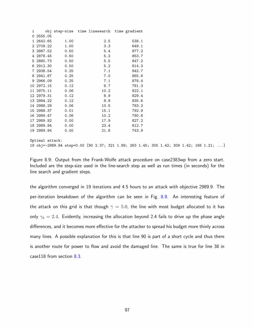
i obj step-size time linesearch time gradient
0 2555.05
1 2642.65 1.00 2.5 538.1
2 2709.22 1.00 3.3 649.1
3 2867.52 0.50 5.4 877.2
4 2878.45 0.50 5.2 853.7
5 2880.73 0.50 5.5 847.2
6 2912.30 0.50 5.2 814.3
7 2938.54 0.25 7.1 842.7
8 2941.87 0.25 7.0 865.6
9 2966.09 0.25 7.1 878.4
10 2972.15 0.12 8.7 781.3
11 2975.11 0.06 10.2 822.1
12 2979.31 0.12 8.9 829.4
13 2984.22 0.12 8.9 835.6
14 2988.29 0.06 10.5 783.3
15 2988.37 0.01 15.1 792.9
16 2989.47 0.06 10.2 790.8
17 2989.92 0.00 17.9 827.2
18 2989.94 0.00 23.4 812.7
19 2989.94 0.00 21.6 743.9
Optimal attack:
19 obj=-2989.94 step=0.00 [90 2.37; 321 1.89; 263 1.45; 305 1.42; 309 1.42; 166 1.21; ...]
Figure 8.9: Output from the Frank-Wolfe attack procedure on case2383wp from a zero start.Included are the step-size used in the line-search step as well as run times (in seconds) for theline search and gradient steps.
the algorithm converged in 19 iterations and 4.5 hours to an attack with objective 2989.9. The
per-iteration breakdown of the algorithm can be seen in Fig. 8.9. An interesting feature of
the attack on this grid is that though γ = 5.0, the line with most budget allocated to it has
only γk = 2.4. Evidently, increasing the allocation beyond 2.4 fails to drive up the phase angle
differences, and it becomes more effective for the attacker to spread his budget more thinly across
many lines. A possible explanation for this is that line 90 is part of a short cycle and thus there
is another route for power to flow and avoid the damaged line. The same is true for line 38 in
case118 from section 8.3.
97
Bibliography
[1] IEEE 118-bus Test System. Electrical and Computer Engineering Department. Illinois Insti-tute of Technology, http://motor.ece.iit.edu/data/IEEE118bus inf/IEEE118bus figure.pdf.
[2] Final Report on the August 14, 2003 Blackout in the United States andCanada: Causes and Recommendations, U.S.-Canada Power Systems Outage TaskForce, 2004. http://energy.gov/oe/downloads/blackout-2003-final-report-august-14-2003-blackout-united-states-and-canada-causes-and.
[3] Integration of Renewable Resources: Transmission and Operating Issues and Recommenda-tions for Integrating Renewable Resources on the California ISO-controlled Grid, CaliforniaISO, 2007. http://www.caiso.com/1ca5/1ca5a7a026270.pdf.
[4] 20% of Wind Energy by 2030: Increasing Wind Energy’s Contribution to US ElectricitySupply, Department of Energy (DOE), 2008. http://energy.gov/eere/wind/20-wind-energy-2030-increasing-wind-energys-contribution-us-electricity-supply.
[5] Arizona-Southern California Outages on September 8, 2011, Federal Energy Regu-latory Commission and the North American Electric Reliability Corporation, 2012.https://www.ferc.gov/legal/staff-reports/04-27-2012-ferc-nerc-report.pdf.
[6] ILOG CPLEX Optimizer, 2012. http://www-01.ibm.com/software/integration/optimization/cplex-optimizer/.
[7] MOSEK Optimizer, 2012. http://www.mosek.com/.
[8] Wind Generation and Total Load in the BPA Balancing Authority, 2012.http://transmission.bpa.gov/business/operations/wind/.
[9] FACT SHEET: Administration Announces New Agenda To Modernize Energy In-frastructure, 2015. https://www.whitehouse.gov/the-press-office/2015/04/21/fact-sheet-administration-announces-new-agenda-modernize-energy-infrastr.
[10] Gurobi Optimizer, 2015. http://www.gurobi.com.
[11] A. Kuzmin, M. Luisier, and O. Schenk, Fast Methods for Computing SelectedElements of the Greens Function in Massively Parallel Nanoelectronic Device Simulations, inEuro-Par 2013 Parallel Processing, F. Wolf, B. Mohr, and D. Mey, eds., vol. 8097 of LectureNotes in Computer Science, Springer Berlin Heidelberg, 2013, pp. 533–544.
98
[12] M. Amin, Turning the Tide on Outages, 2010.http://www.greentechmedia.com/articles/read/turning-the-the-tide-on-outages.
[13] G. Andersson, Modelling and analysis of electric power systems, EEH - Power SystemsLaboratory, (2008).
[14] J. M. Arroyo and F. D. Galiana, On the solution of the bilevel programming for-mulation of the terrorist threat problem, IEEE Transactions on Power Systems, 20 (2005),pp. 789–797.
[15] C. Audet, S. Le Digabel, and C. Tribes, NOMAD User Guide, 2009.https://www.gerad.ca/nomad/Downloads/user guide.pdf.
[16] S. S. Baghsorkhi and I. A. Hiskens, Analysis tools for assessing the impact of windpower on weak grids, SysCon, (2012), pp. 1–8.
[17] A. Bergen and V. Vittal, Power Systems Analysis, Prentice Hall, 2nd ed., 2000.
[18] D. Bienstock, Electrical Transmission System Cascades and Vulnerability, Society forIndustrial and Applied Mathematics, Philadelphia, PA, 2015.
[19] D. Bienstock, M. Chertkov, and S. Harnett, Chance-Constrained Optimal PowerFlow: Risk-Aware Network Control under Uncertainty, SIAM Review, 56 (2014), pp. 461–495.
[20] D. Bienstock and A. Verma, The N - k problem in power grids: New models, formula-tions, and numerical experiments, SIAM Journal on Optimization, 20 (2010), pp. 2352–2380.
[21] S. Boyd and L. Vandenberghe, Convex Optimization, Cambridge University Press,2004.
[22] W. A. Bukhsh, A. Grothey, K. I. M. McKinnon, and P. A. Trodden, LocalSolutions of the Optimal Power Flow Problem, IEEE Transactions on Power Systems, 28(2013), pp. 4780–4788.
[23] M. B. Cain, R. P. O’Neill, and A. Castillo, History of Optimal Power Flow andFormulations, Federal Energy Regulatory Commission. . . . , (2012), pp. 1–36.
[24] M. D. Canon and C. D. Cullum, A Tight Upper Bound on the Rate of Convergenceof Frank-Wolfe Algorithm, SIAM Journal on Control, 6 (1968).
[25] A. Charnes, W. W. Cooper, and G. H. Symonds, Cost horizons and certaintyequivalents: an approach to stochastic programming of heating oil, Management Science, 4(1958), pp. 235–263.
[26] M. Chertkov, F. Pan, and M. Stepanov, Predicting Failures in Power Grids: TheCase of Static Overloads, IEEE Transactions on Smart Grids, 2 (2010), p. 150.
99
[27] M. Chertkov, M. Stepanov, F. Pan, and R. Baldick, Exact and efficient al-gorithm to discover extreme stochastic events in wind generation over transmission PowerGrids, CDC-ECC, (2011), pp. 2174–2180.
[28] B. Colson, P. Marcotte, and G. Savard, An overview of bilevel optimization,Annals of Operations Research, 153 (2007), pp. 235–256.
[29] C. DeMarco and T. Overbye, Low voltage power flow solutions and their role inexit time based security measures for voltage collapse, in Proceedings of the 27th IEEEConference on Decision and Control, IEEE, 1988, pp. 2127–2131.
[30] I. Dobson and H.-D. Chiang, Towards a Theory of Voltage Collapse in Electric PowerSystems, Systems and Control Letters, 13 (1989), pp. 253–262.
[31] V. Donde, V. Lopez, B. Lesieutre, A. Pinar, C. Yang, and J. Meza, Se-vere multiple contingency screening in electric power systems, IEEE Transactions on PowerSystems, 23 (2008), pp. 406–417.
[32] M. Frank and P. Wolfe, An algorithm for quadratic programming, Naval ResearchLogistics Quarterly, 3 (1956), pp. 95–110.
[33] V. Frolov, S. Backhaus, and M. Chertkov, Reinforcing Power Grid Transmissionwith FACTS Devices, arxiv:1307.1940, (2013).
[34] E. R. Gansner and S. C. North, An open graph visualization system and its applica-tions to software engineering, Software - Practice and Experience, 30 (2000), pp. 1203–1233.
[35] D. Goldfarb and F. Alizadeh, Second-Order Cone Programming, Mathematical Pro-gramming, 95 (2003), pp. 3–51.
[36] M. Grotschel, L. Lovasz, and A. Schrijver, Geometric Algorithms and Combi-natorial Optimization, Springer-Verlag, 1998.
[37] R. Hooke and T. A. Jeeves, ”Direct Search” Solution of Numerical and StatisticalProblems, Journal of the ACM, 8 (1961), pp. 212–229.
[38] M. Jaggi, Revisiting Frank-Wolfe: Projection-free sparse convex optimization, 30th Inter-national Conference on Machine Learning, (2013), pp. 427–435.
[39] A. Juditsky and A. Nemirovski, First-Order Methods for Nonsmooth Convex Large-Scale Optimization, I: General Purpose Methods, in Optimization for Machine Learning,S. Sra, S. Nowozin, and S. Wright, eds., The MIT Press, 2012, pp. 121–48.
[40] J. Kelley, The Cutting-Plane Method for Solving Convex Programs, Journal of the Societyfor Industrial and Applied Mathematics, 8 (1960), pp. 703–712.
[41] T. Kim, S. J. Wright, D. Bienstock, and S. Harnett, Vulnerability Analysis ofPower Systems, arXiv:1503.02360, (2015).
100
[42] M. Kleimaier and H. Weber, Grid Integration of Wind Generation, in InternationalConference on Large High Voltage Electric Systems, CIGRE, 2009. Technical brochure 450.
[43] A. Klos and J. Wojcicka, Physical aspects of the nonuniqueness of load flow solutions,International Journal of Electrical Power & Energy Systems, 13 (1991), pp. 268–276.
[44] B. Kocuk, S. S. Dey, and X. A. Sun, Inexactness of SDP relaxation and valid inequal-ities for optimal power flow, IEEE Transactions on Power Systems, 31 (2014), pp. 642–651.
[45] , Strong SOCP Relaxations for Optimal Power Flow, arxiv:1504.06770, (2015).
[46] J. Lavaei and S. Low, Zero Duality Gap in Optimal Power Flow Problem, IEEE Trans-actions on Power Systems, 27 (2012), pp. 92–107.
[47] S. H. Low, Convex Relaxation of Optimal Power Flow. Part II: Exactness, IEEE Transac-tions on Control of Network Systems, 1 (2014), pp. 1–1.
[48] , Convex Relaxation of Optimal Power FlowPart I: Formulations and Equivalence, IEEETransactions on Control of Network Systems, 1 (2014), pp. 15–27.
[49] Y. V. Makarov, C. Loutan, J. Ma, and P. de Mello, Operational Impacts ofWind Generation on California Power Systems, Power Systems, IEEE Transactions on, 24(2009), pp. 1039–1050.
[50] L. B. Miller and H. Wagner, Chance-constrained programming with joint constraints,Operations Research, 13 (1965), pp. 930–945.
[51] D. Molzahn, Application of Semidefinite Optimization Techniques to Problems in ElectricPower Systems, PhD thesis, University of Wisconsin-Madison, 2013.
[52] E. C. Morgan, M. Lackner, R. M. Vogel, and L. G. Baise, Probability distribu-tions for offshore wind speeds, Energy Conversion and Management, 52 (2011), pp. 15–26.
[53] A. L. Motto, J. M. Arroyo, and F. D. Galiana, A mixed-integer LP procedurefor the analysis of electric grid security under disruptive threat, IEEE Transactions on PowerSystems, 20 (2005), pp. 1357–1365.
[54] A. Nemirovski and A. Shapiro, Convex Approximations of Chance Constrained Pro-grams, SIAM Journal on Optimization, 17 (2006), pp. 969–996.
[55] J. Nocedal and S. J. Wright, Numerical Optimization, vol. 43 of Springer Series inOperations Research, Springer, 1999.
[56] U. A. Ozturk and M. Mazumdar, A solution to the stochastic unit commitmentproblem using chance constrained programming, Power Systems, IEEE, 19 (2004), pp. 1589–1598.
[57] A. Pinar, J. Meza, V. Donde, and B. Lesieutre, Optimization Strategies for theVulnerability Analysis of the Electric Power Grid, SIAM Journal on Optimization, (2010).
101
[58] A. Prekopa, On probabilistic constrained programming, Proc. Princeton Symposium onMath. Programming, (1970), pp. 113–138.
[59] F. Salam, L. Ni, S. Guo, and X. Sun, Parallel processing for the load flow of powersystems: the approach and applications, in Proceedings of the 28th IEEE Conference onDecision and Control, IEEE, 1989, pp. 2173–2178.
[60] J. Salmeron, K. Wood, and R. Baldick, Analysis of electric grid security underterrorist threat, IEEE Transactions on Power Systems, 19 (2004), pp. 905–912.
[61] O. Schenk, M. Bollhofer, and R. A. Romer, On Large-Scale DiagonalizationTechniques for the Anderson Model of Localization, SIAM Rev., 50 (2008), pp. 91–112.
[62] O. Schenk, A. Wachter, and M. Hagemann, Matching-based preprocessing al-gorithms to the solution of saddle-point problems in large-scale nonconvex interior-pointoptimization, Computational Optimization and Applications, 36 (2007), pp. 321–341.
[63] J. F. Sturm, Using SeDuMi 1.02, A Matlab toolbox for optimization over symmetriccones, Optimization Methods and Software, 11 (1999), pp. 625–653.
[64] R. H. Tutuncu, K. C. Toh, and M. J. Todd, Solving semidefinite-quadratic-linearprograms using SDPT3, Mathematical Programming, Series B, 95 (2003), pp. 189–217.
[65] M. Vrakopoulou, K. Margellos, J. Lygeros, and G. Andersson, A proba-bilistic framework for security constrained reserve scheduling of networks with wind powergeneration, in Energy Conference and Exhibition (ENERGYCON), 2012 IEEE International,2012, pp. 452–457.
[66] A. Wachter and L. T. Biegler, On the implementation of an interior-point filterline-search algorithm for large-scale nonlinear programming, Mathematical Programming,106 (2006), pp. 25–57.
[67] G. Wang, M. Negrete-Pincetic, A. Kowli, E. Shafieepoorfard, S. Meyn,and U. Shanbhag, Dynamic Competitive Equilibria in Electricity Markets, in Control andOptimization Theory for Electric Smart Grids, A. Chakrabortty and M. Illic, eds., Springer,2011.
[68] H. Wang, C. E. Murillo-Sanchez, R. D. Zimmerman, and R. J. Thomas, OnComputational Issues of Market-Based Optimal Power Flow, IEEE Transactions on PowerSystems, 22 (2007), pp. 1185–1193.
[69] J. Wang, M. Shahidehpour, and Z. Li, Security-Constrained Unit CommitmentWith Volatile Wind Power Generation, Power Systems, IEEE Transactions on, 23 (2008),pp. 1319–1327.
[70] H. Zhang, Chance Constrained Programming for Optimal Power Flow Under Uncertainty,Power Systems, IEEE Transactions on, 26 (2011), pp. 2417–2424.
102

[71] S. Zhang, Y. Song, Z. Hu, and L. Yao, Robust optimization method based onscenario analysis for unit commitment considering wind uncertainties, in Power and EnergySociety General Meeting, 2011 IEEE, jul 2011, pp. 1–7.
[72] R. Zimmerman, C. Murillo Sanchez, and R. Thomas, MATPOWER: Steady-State Operations, Planning, and Analysis Tools for Power Systems Research and Education,Power Systems, IEEE Transactions on, 26 (2011), pp. 12–19.
103