Optimization-based Motion Planning and Optimal Control

Optimization-based Motion Planning and OptimalControl

Jun Zeng

Department of Mechanical EngineeringUniversity of California, Berkeley

February 25th 2020

Jun Zeng (UC Berkeley) February 25th 2020 1 / 33

Overview

1 Introduction

2 Optimization-based path planningGeneral methodsExamples

3 Optimal controlModel predictive control


1 Introduction




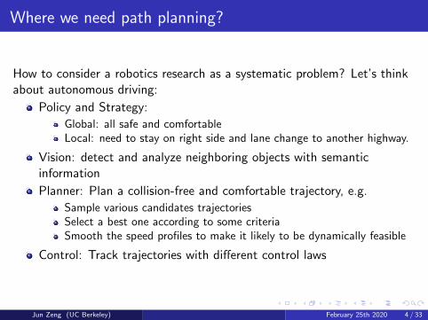
Where we need path planning?

How to consider a robotics research as a systematic problem? Let’s thinkabout autonomous driving:

Policy and Strategy:

Global: all safe and comfortableLocal: need to stay on right side and lane change to another highway.

Vision: detect and analyze neighboring objects with semanticinformation

Planner: Plan a collision-free and comfortable trajectory, e.g.

Sample various candidates trajectoriesSelect a best one according to some criteriaSmooth the speed profiles to make it likely to be dynamically feasible

Control: Track trajectories with different control laws


Planning is the bridge between high-level and low-level.

Need to consider noise and disturbance from vision module

Make the trajectory dynamically-feasible for the control module andother low-level ones.

The performance of path planning is generally determined by two aspectsfrom my personal perspective:

Refresh rate: already a huge time delay from various vision sensors,e.g. you wouldn’t expect the refresh rate to be less than 10Hz forautonomous driving.

Correctness: RRT without smoothness is generally hard to track...


Optimal Control vs Optimization-based Path Planning

Optimal control: linear–quadratic regulator (LQR), model predictivecontrol (MPC), sliding mode control, etc.

Topics in optimization-based path planning:

Speed profile smoothing: e.g. minimum-jerk in autonomous driving.Contact force: e.g. hybrid mode switch with contact force in leggedrobotics.Energy efficiency: e.g. minimum-snap/jerk in aerial robotics.

They are the same in mathematics: an optimization problem isformulated to generate control strategy or trajectory/robot’s motions.

They are different in the implementation: optimal control is usuallyholding a higher refresh rate and needs to be solved very fast, whilethe optimization problem in planning isn’t necessarily to be solvedcomputationally with that fast rate.


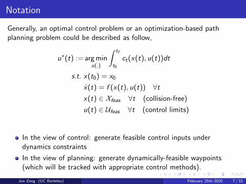
Notation

Generally, an optimal control problem or an optimization-based pathplanning problem could be described as follow,

u∗(t) := arg minu(.)

∫ tf

t0

ct(x(t), u(t))dt

s.t. x(t0) = x0

x(t) = f (x(t), u(t)) ∀tx(t) ∈ Xfeas ∀t (collision-free)

u(t) ∈ Ufeas ∀t (control limits)

In the view of control: generate feasible control inputs underdynamics constraints

In the view of planning: generate dynamically-feasible waypoints(which will be tracked with appropriate control methods).


1 Introduction




Mathematical methods

Generally, a optimization problem will satisfy a variety of constraints, thisleads us to have different methods to solve them numerically.Some of them have explicit solutions:

convex quadratic programming (Convex QP)

LQR: For continuous-system linear system x = Ax + Bu with aquadratic cost J =

∫∞0 (xTQx + uTRu + 2xTNu)dt. The feedback

control law to minimize the value of the cost is u = −Kx , whereK = R−1(BTP + NT ) andATP + PA− (PB + N)R−1(BTP + NT ) + Q = 0. Here, the controllaw could be solved explicitly.


Numerical methods

Other general problems don’t have explicit solutions and don’t guaranteeexisting solution but could be solved numerically:An optimization-based path planning problem could be formulated asseveral types:

Shooting methods: we ’shoot’ out trajectories in different directionsuntil we find a trajectory that has the desired boundary value.

Collocation methods: choose a finite-dimensional space of candidatesolutions (e.g. polynomials) and a number of points in the domain(called collocation points), and to select that solution which satisfiesthe given equation at the collocation points.


Solvers and existence of solutions

Most likely, all problems could be formulated into a dynamic programmingproblem and could be solved with various numerical solvers1:

for convex problems:

software: CVX, OSQPinternal solvers: Gurobi, Sedumi, Mosek

for non-convex problems:

interior point: IPOPT, SNOPTactive set method: SAS

We are more interested in the existence of the solution of theoptimization. For a convex problem, we are likely to ensure at least onesolution (might have several ones if it’s nonlinear or non-convex costfunction, our numerical solution will depends on the initial point where wedo gradient descent). But for general non-convex problem, we are unableto guarantee the existence of solution.

1More mathematical details for solving optimization problem are presented in EE 227A/B/C.


Trajectory smoothing

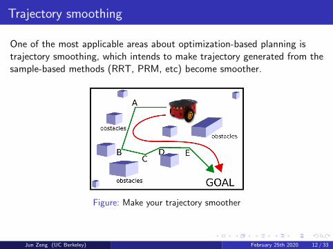
One of the most applicable areas about optimization-based planning istrajectory smoothing, which intends to make trajectory generated from thesample-based methods (RRT, PRM, etc) become smoother.

Figure: Make your trajectory smoother


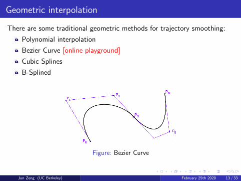
Geometric interpolation

There are some traditional geometric methods for trajectory smoothing:

Polynomial interpolation

Bezier Curve [online playground]

Cubic Splines

B-Splined

Figure: Bezier Curve


https://www.geogebra.org/m/r3UWE9KR

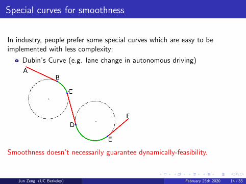
Special curves for smoothness

In industry, people prefer some special curves which are easy to beimplemented with less complexity:

Dubin’s Curve (e.g. lane change in autonomous driving)

Smoothness doesn’t necessarily guarantee dynamically-feasibility.


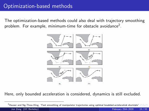
Optimization-based methods

The optimization-based methods could also deal with trajectory smoothingproblem. For example, minimum-time for obstacle avoidance2.

Here, only bounded acceleration is considered, dynamics is still excluded.

2Hauser and Ng-Thow-Hing, “Fast smoothing of manipulator trajectories using optimal bounded-acceleration shortcuts”.


Related work

”Time Elastic Band” planner (TEB Planner) with ROS integration isintroduced34, where non-holonomic kinematics is considered, butroughtly. [demo video in ROS]

For autonomous driving, some special techniques are alsoproposed567.

3Rosmann et al., “Trajectory modification considering dynamic constraints of autonomous robots”.4Rosmann et al., “Efficient trajectory optimization using a sparse model”.5Dolgov et al., “Path planning for autonomous vehicles in unknown semi-structured environments”.6Ziegler et al., “Trajectory planning for Bertha—A local, continuous method”.7Gu and Dolan, “On-road motion planning for autonomous vehicles”.


https://www.youtube.com/watch?v=e1Bw6JOgHME&feature=emb_title

There are many work about this area, the pipeline of path planning ismainly considered as trajectory generation + trajectory smooth, and theproblem is formulated to consider mobile robots not holding too complexdynamics (autonomous cars, robot arm, etc).

How about generating a dynamically-feasible trajectory directly from anoptimization-based problem? There are several tricky points to take intoaccount.

Obstacle avoidance and Safety

Hybrid mode switch (contact force)

Energy efficiency and smoothness (e.g. which kind of cost functionwe shall choose)


Obstacle avoidance

There are several ways to consider obstacle avoidance as constraints in anoptimization-based problem:

simple geometric constraints: e.g. (x − xobs)2 + (y − yobs)2 ≥ r2

very rough consideration: point-mass and round obstaclenonlinear and non-convex constraintsit could be solved with modern solvers (IPOPT, etc) but doesn’tguarantee a solution.


Obstacle avoidance

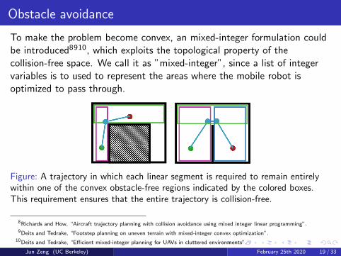
To make the problem become convex, an mixed-integer formulation couldbe introduced8910, which exploits the topological property of thecollision-free space. We call it as ”mixed-integer”, since a list of integervariables is to used to represent the areas where the mobile robot isoptimized to pass through.

Figure: A trajectory in which each linear segment is required to remain entirelywithin one of the convex obstacle-free regions indicated by the colored boxes.This requirement ensures that the entire trajectory is collision-free.

8Richards and How, “Aircraft trajectory planning with collision avoidance using mixed integer linear programming”.9Deits and Tedrake, “Footstep planning on uneven terrain with mixed-integer convex optimization”.

10Deits and Tedrake, “Efficient mixed-integer planning for UAVs in cluttered environments”.


Obstacle avoidance

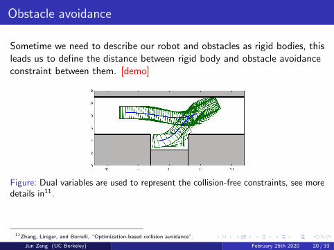
Sometime we need to describe our robot and obstacles as rigid bodies, thisleads us to define the distance between rigid body and obstacle avoidanceconstraint between them. [demo]

Figure: Dual variables are used to represent the collision-free constraints, see moredetails in11.

11Zhang, Liniger, and Borrelli, “Optimization-based collision avoidance”.


https://raw.githubusercontent.com/XiaojingGeorgeZhang/OBCA/master/images/TrajBack_ParkingVideo.gif

Obstacle avoidance

There are many other famous work:

Sequential Convex Optimization12

STOMP13: deployed on PR2 robot and recommended by ROS.

CHOMP14: consider waypoint optimization and trajectory smoothness

12Schulman et al., “Motion planning with sequential convex optimization and convex collision checking”.13Kalakrishnan et al., “STOMP: Stochastic trajectory optimization for motion planning”.14Zucker et al., “Chomp: Covariant hamiltonian optimization for motion planning”.


Other work

There are other famous work for special systems:

Swarm path planning for UAV15

Baidu Apollo open source planner16

15Roberge, Tarbouchi, and Labonte, “Comparison of parallel genetic algorithm and particle swarm optimization for real-timeUAV path planning”.

16Fan et al., “Baidu apollo em motion planner”.


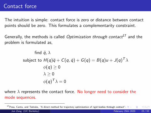
Contact force

The intuition is simple: contact force is zero or distance between contactpoints should be zero. This formulates a complementarity constraint.

Generally, the methods is called Optimization through contact17 and theproblem is formulated as,

find q, λ

subject to H(q)q + C (q, q) + G (q) = B(q)u + J(q)Tλ

φ(q) ≥ 0

λ ≥ 0

φ(q)Tλ = 0

where λ represents the contact force. No longer need to consider themode sequences.

17Posa, Cantu, and Tedrake, “A direct method for trajectory optimization of rigid bodies through contact”.


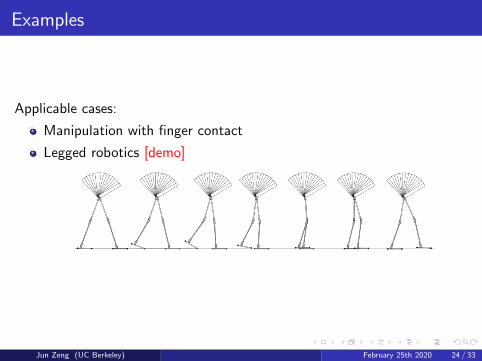
Examples

Applicable cases:

Manipulation with finger contact

Legged robotics [demo]


https://www.youtube.com/watch?v=pH1pDXnCBx4

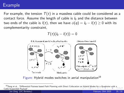
Example

For example, the tension T (t) in a massless cable could be considered as acontact force. Assume the length of cable is l0 and the distance betweentwo ends of the cable is l(t), then we have φ(q) = l0 − l(t) ≥ 0 with itscomplementarity constraint,

T (t)(l0 − l(t)) = 0

Figure: Hybrid modes switches in aerial manipulation18

18Zeng et al., “Differential Flatness based Path Planning with Direct Collocation on Hybrid Modes for a Quadrotor with aCable-Suspended Payload”.


Energy efficiency and smoothness

A cost function to minimize jerk (third-order derivative of vehicle’sposition)19.

A cost function to minimize snap (fourth-order derivative of vehicle’sposition)20.

Actually, people find that minimum jerk or snap usually performed betterthan those of other orders in robots for smoothness.

19Pattacini et al., “An experimental evaluation of a novel minimum-jerk cartesian controller for humanoid robots”.20Mellinger and Kumar, “Minimum snap trajectory generation and control for quadrotors”.


Discussion

The optimization-based path planning is still active research topic, thereare many existing problems which need to be solved:

multi-agents: e.g. ensure collision-free movements in drone swarm

safety: e.g. guarantee safety-critical trajectory in a noisy environment(sensor noise, model uncertainty, algorithm bias, etc)

policy: centralized/decentralized, human-robot interaction


1 Introduction




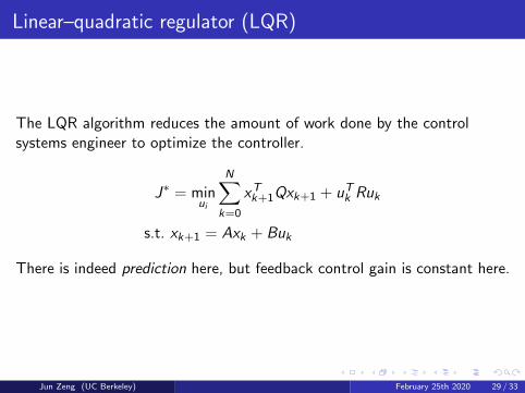
Linear–quadratic regulator (LQR)

The LQR algorithm reduces the amount of work done by the controlsystems engineer to optimize the controller.

J∗ = minui

N∑k=0

xTk+1Qxk+1 + uTk Ruk

s.t. xk+1 = Axk + Buk

There is indeed prediction here, but feedback control gain is constant here.


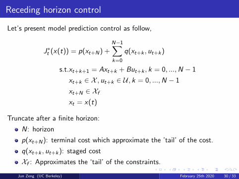
Receding horizon control

Let’s present model prediction control as follow,

J∗t (x(t)) = p(xt+N) +N−1∑k=0

q(xt+k , ut+k)

s.t.xt+k+1 = Axt+k + But+k , k = 0, ...,N − 1

xt+k ∈ X , ut+k ∈ U , k = 0, ...,N − 1

xt+N ∈ Xf

xt = x(t)

Truncate after a finite horizon:

N: horizon

p(xt+N): terminal cost which approximate the ’tail’ of the cost.

q(xt+k , ut+k): staged cost

Xf : Approximates the ‘tail’ of the constraints.


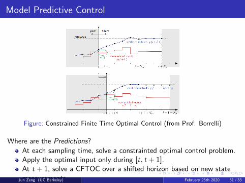
Model Predictive Control

Figure: Constrained Finite Time Optimal Control (from Prof. Borrelli)

Where are the Predictions?

At each sampling time, solve a constrainted optimal control problem.Apply the optimal input only during [t, t + 1].At t + 1, solve a CFTOC over a shifted horizon based on new statemeasurements.Jun Zeng (UC Berkeley) February 25th 2020 31 / 33

Open-loop vs Closed-loop

Some definitions among researchers working on MPC:

Open-loop trajectory: at each time step, we have a constraintedoptimal control problem, which solves a feasible trajectory withpredictions.

Closed-loop trajectory: since we solve optimal control problem ateach time step, the robot will moves along a closed-loop trajectorywith this control policy.


Discussions

Terminal cost ensures the Lyapunov convergence, but it’s notnecessary.

Larger horizon brings a bigger controllable set, but needs more timeto calculate the optimization.

The dynamics constraints could be nonlinear, which will make theproblem as a dynamic programming problem.

There are many variants of MPC: Robust MPC, Adaptive MPC, MPCwith obstacle avoidance, etc.

Recent work about Learning MPC takes safety into account. [demo]


https://www.youtube.com/watch?v=W4LkQaTvzhI&feature=emb_title

Documents

Optimization-based Motion Planning and Optimal Control