Embed Size (px)
Citation preview
Optimisation of TPDS Supply Chain | P 1
PROOF OF CONCEPT 2018
World Food Programme
OPTIMISATION OF SUPPLY CHAIN OF TARGETED PUBLIC DISTRIBUTION SYSTEMIN DHENKANAL, ODISHA

P 2 |
Team Members: Mr. Sergio Silva, Supply Chain Officer (R&D), OSCP, WFP Headquarters RomeMr. Luis Anjos, Supply Chain Officer, OSCP, WFP Headquarters RomeMr. Koen Peters, Supply Chain Officer, OSCP, WFP Headquarters RomeMr. Wouter Smeenk, Supply Chain Officer, OSCP, WFP Headquarters RomeMr. Ankit Sood, Programme Policy Officer and Head of System Reforms, WFP IndiaMs. Esha Singh, Programme Policy Officer, WFP IndiaMr. Himanshu Bal, State Project Coordinator, Odisha, WFP India
Disclaimer:
All rights reserved. Reproduction and dissemination of material in this information product for educational or other non-commercial uses is authorized without any prior written permission from the copyright holders provided the source is fully acknowledged. Reproduction of material in this information product for resale or other commercial purposes is prohibited without written permission. Applications for such permission should be addressed to the Communications Division of the World Food Programme.
© WFP 2018
For more information, please contact
World Food Programme2, Poorvi Marg, Vasant Vihar, New Delhi-110057Tel: +91-46554000E-mail- [email protected]
Optimisation of TPDS Supply Chain | P 3
OPTIMISATION OF TPDS SUPPLY CHAIN
DHENKANAL, ODISHAPROOF OF CONCEPT, 2018


Acknowledgement
The World Food Programme (WFP) is the largest humanitarian organisation working in emergencies and development contexts supporting over 80 million people worldwide through essential food, school meals, cash transfers and technical assistance. To ensure that we deliver every day in over 80 countries, supply chain plays an integral role; supporting the entire process of end-to-end planning, procuring and delivering assistance.
Inline with our efforts in ensuring a smooth, well functioning and efficient supply chain, WFP have been investing in innvoting and developing solutions that help optimise our supply chains to reduce operational, administrative and financial costs. This proof of concept for optimisation of the supply chain of TPDS in Dhenkanal, Odisha is a step in the same direction.
I would like to express my gratitude to the Food Supplies and Consumer Welfare Department (FS&CWD), Odisha led by Mr. Vir Vikram Yadav, Secretary (FS&CWD) for their support in completing this activity. I would also like to congratulate Mr. Yadav and his team for their initiate to pioneer optimisation of supply chains in TPDS in India, which I hope will serve as a guide to other states.
Lastly, a special gratitude to the Supply Chain and Planning team in WFP, Rome and the System Reforms Unit in WFP, India for conceptualising and implementing various scenarios to optimise the exsiting supply chain. I am happy to share this report which details the process, methodology and results of the optimisation of TPDS for Dhenkanal, Odisha.
Mahadevan Ramachandran
Chief, Supply Chain Planning and Retail Supply Chains, WFP

P 6 |

Optimisation of TPDS Supply Chain | P 7

P 8 |

Optimisation of TPDS Supply Chain | P 9
Hameed NuruRepresentative and Country Director
WFP, India
Foreword
The United Nations World Food Programme (WFP) has been working closely with the Government of India since 1963, supporting the Government in its endeavor to provide food and nutrition security to the most vulnerable. Over the decades, WFP’s role has evolved from a food aid agency to a technical partner for the Government. WFP’s association with the Government of Odisha was initiated in 2007 and in the recent years, WFP has supported the state government in implementation of the National Food Security Act, 2013 and in the transformation of its Targeted Public Distribution System (TPDS) to be fully digitized and automated, enabling it to become more transparent, accountable and efficient.
In line with this initiative, WFP undertook an assessment in collaboration with the Government of Odisha in 2017, to review the procurement and supply chain system as well as of the Paddy Procurement Automation System (P-PAS) and Supply Chain Management System (SCMS) solutions of TPDS in the state. The assessment report recommended a business process review of the existing P-PAS and SCMS systems to enhance and integrate the two, as well as the optimization of the entire supply chain to make it more efficient and reduce underutilization of resources.
Based on the recommendations of the report and on Government of Odisha’s request, an assessment was conducted in early 2018 to determine optimization opportunities in Odisha and collect data for establishing a Proof of Concept (PoC) for optimization of the supply chain. Dhenkanal district of Odisha, which has 9,28,000 TPDS beneficiaries out of 3.26 crores in Odisha was chosen for the PoC.
The aim of this PoC is to demonstrate the savings potential through optimizing the supply chain by applying WFP’s operations research approach and tools, leading to efficiency improvements in the procurement, storage and delivery of food grains. The PoC analyses different scenarios and finds that in a fully optimized scenario, cost savings of 29 per cent on the current costs can be achieved.
This process has enormous potential to turn underutilization of resources into assets and savings, which can be further used to reach the beneficiaries more effectively and help them gain more from the TPDS. I hope this analysis will be helpful for the Government of Odisha in creating an optimized supply chain network across the state to better manage food grain flows for all food safety nets in Odisha.
I would like to congratulate the Government of Odisha for its commitment and remarkable progress in building an efficient public distribution system and introducing cutting edge technology to the entire value chain from procurement to distribution. WFP looks forward to a continued and strong partnership with the Government of Odisha, towards the common objective to improve access to safe and nutritious food for all.

P 10 |

Optimisation of TPDS Supply Chain | P 11
ContentsList of abbreviations ......................................................................................................................15
Table of conversion ........................................................................................................................ 16
Key definitions ............................................................................................................................... 16
1. Executive summary ...................................................................................................................18
1.1. Key findings ................................................................................................................... 18
2. Introduction ............................................................................................................................... 24
2.1. Key objectives ................................................................................................................ 25
2.2. Approach and methodology ......................................................................................... 26
2.3. Data sources ................................................................................................................. 26
2.4. Optimisation model ........................................................................................................ 27
2.5. Scenarios ....................................................................................................................... 28
2.6. Key outputs and outcomes ............................................................................................ 28
2.7. Limitations of the model and analysis............................................................................ 30
3. Baseline ..................................................................................................................................... 34
3.1. About the scenario ......................................................................................................... 34
3.2. Key constriants .............................................................................................................. 34
3.3. Summary statistics ....................................................................................................... 35
3.4. Key performance indicators ........................................................................................... 35
3.4.1. Observations for leg 1: PACS to Mill .................................................................. 36
3.4.2. Observations for leg 2: Mill to RRC, FCI to RRC ............................................... 37
3.4.3. Observations for leg 3: RRC to FPS ................................................................. 38
3.4.4. Geospatial representation of the supply chain network in baseline ................. 39
4. Scenario 1. Baseline with change in transport contracting ..................................................42
4.1. About the scenario ......................................................................................................... 42
4.2. Key performance indicators ........................................................................................... 43
4.3. Changes from the baseline tagging and volume ........................................................... 44
4.4. Changes required to implement this scenario ............................................................... 44
5. Scenario 2. Optimise PACS tagging .........................................................................................46
5.1. About the scenario ......................................................................................................... 46
5.2. Key constraints .............................................................................................................. 46

P 12 |
5.3. Key performance indicators ........................................................................................... 47
5.4. Changes from the baseline ............................................................................................ 48
5.4.1. Observations for leg 1: PACS to Mill .................................................................. 48
5.4.2. Geospatial representation of the supply chain network in the optimising
PACS tagging scenario ...................................................................................... 50
5.5. Changes required to implement this scenario ............................................................... 50
6. Scenario 3. Optimise leg 1 and 2 .............................................................................................52
6.1. About the scenario ......................................................................................................... 52
6.2. Key constraints .............................................................................................................. 52
6.3. Key performance indicators .....................................................................................................53
6.4. Changes from the baseline ............................................................................................ 54
6.4.1. Observations for leg 2: Mill to RRC ................................................................... 55
6.4.2. Geospatial representation of the supply chain network in optimising leg 1
and 2 .................................................................................................................. 56
6.5. Changes required to implement the scenario ................................................................ 57
7. Scenario 4. Optimise FPS tagging ...........................................................................................60
7.1. About the scenario ......................................................................................................... 60
7.2. Key constraints .............................................................................................................. 60
7.3. Key performance indicators ........................................................................................... 61
7.4. Changes from the baseline ............................................................................................ 62
7.4.1. Observations for leg 3: RRC to FPS .................................................................. 62
7.4.2. Geospatial representation of the supply chain network in optimising
FPS tagging ....................................................................................................... 64
7.5. Changes required to implement this scenario .............................................................. 65
8. Scenario 5. Closing Mills .......................................................................................................... 68
8.1. About the scenario ......................................................................................................... 68
8.2. Key constraint ................................................................................................................ 68
8.3. Key performance indicators ........................................................................................... 69
8.4. Changes from the baseline ............................................................................................ 70
8.4.1. Observations for leg 1: PACS to Mill .................................................................. 70
8.4.2. Observations for leg 2: Mill to RRC ................................................................... 71
8.4.3. Geospatial representation of the supply chain network in closing mills
scenario.............................................................................................................. 72
8.5. Changes required to implement this scenario ............................................................... 73
9. Scenario 6. Closing PACS ......................................................................................................... 76
9.1. About the scenario ......................................................................................................... 76

Optimisation of TPDS Supply Chain | P 13
9.2. Key constriants .............................................................................................................. 76
9.3. Key performance indicators ........................................................................................... 77
9.4. Changes from the baseline ............................................................................................ 78
9.4.1. Observations for leg 1: PACS to Mill .................................................................. 78
9.4.2. Geospatial representation of the supply chain network in the closing
PACS scenario ................................................................................................... 79
9.5. Changes required to implement this scenario ............................................................... 80
10. Scenario 7. Closing FPS .......................................................................................................... 82
10.1. About the scenario ......................................................................................................... 82
10.2. Key constriants .............................................................................................................. 82
10.3. Key performance indicators ........................................................................................... 83
10.4. Changes from the baseline ............................................................................................ 84
10.4.1. Observations for leg 3: RRC TO FPS ................................................................. 84
10.5. Changes required to implement the scenario ............................................................... 86
11. Scenario 8. Fully optimised with capacity constraint ..........................................................88
11.1. About the scenario ......................................................................................................... 88
11.2. Key constriants .............................................................................................................. 88
11.3. Key performance indicators ........................................................................................... 89
11.4. Changes from the baseline ............................................................................................ 90
11.4.1. Observations for leg 1: PACS to Mill .................................................................. 90
11.4.2. Observations for leg 2: Mill to RRC ................................................................... 91
11.4.3. Observations for leg 3: RRC to FPS .................................................................. 93
11.4.4. Geospatial representation of the supply chain network in the fully optimised
with capacity constrained scenario ................................................................... 94
11.5. Changes required to implement the scenario ............................................................... 96
12. Scenario 9. Fully optimised with capacity constraint (+15%) .............................................98
12.1. About the scenario ......................................................................................................... 98
12.2. Key constriants .............................................................................................................. 98
12.3. Key performance indicators ........................................................................................... 99
12.4. Changes from the baseline ......................................................................................... 100
12.4.1. Observations for leg 1: PACS to Mill ................................................................ 100
12.4.2. Observations for leg 2: Mill to RRC and FCI to RRC ....................................... 101
12.4.3. Observations for leg 3: RRC to FPS ................................................................ 103
12.4.4. Geospatial representation of the supply chain network in the fully optimised
with capacity constrained +15% scenario ....................................................... 104
12.5. Changes required to implement the scenario ............................................................. 105

P 14 |
13. Scenario 10. Fully optimised ...............................................................................................108
13.1. About the scenario ....................................................................................................... 108
13.2. Key constriants ............................................................................................................ 108
13.3. Key performance indicators ......................................................................................... 109
13.4. Changes from the baseline .......................................................................................... 110
13.4.1. Observations for leg 1: PACS to Mill ................................................................ 110
13.4.2. Observations for leg 2: Mill to RRC and FCI to RRC ....................................... 111
13.4.3. Distance and costs .......................................................................................... 111
13.4.4. Geospatial representation of the supply chain network in the fully optimised 113
13.5. Changes required to implement the scenario .............................................................. 115
Annexures .....................................................................................................................................117
Annexure 1: list of figures ......................................................................................................... 118
Annexure 2: list of tables .......................................................................................................... 121

Optimisation of TPDS Supply Chain | P 15
LIST OF ABBREVIATIONSCTC - Change in Transport Contracting
EtE - End-to-End
FCI - Food Corporation of India
FPS - Fair Price Shop
FSCW - Food Supplies and Consumer Welfare Department
GMP - Good Manufacturing Practices
GoO - Government of Odisha
KPI - Key Performance Indicator
MSP - Minimum Support Price
NFSA - National Food Security Act
PACS - Primary Agriculture Credit Society
PoC - Proof of Concept
P-PAS - Paddy Procurement Automation System
PPC - Paddy Purchase Centre
RRC - Rice Receiving Centre
SCMS - Supply Chain Management System
SHF - Small Holder Farmers
TPDS - Targeted Public Distribution System
WFP - World Food Programme
MILLSMill1 - Annapurna Rice Mill
Mill2 - BDN Food Products
Mill3 - Bhutia Foods Pvt. Ltd.
Mill4 - Harpriya Rice Mill
Mill5 - Kamlesh Rice Mill
Mill6 - Laxminarayan Agro Foods
Mill7 - Maa Kamakhi Food Processor
Mill8 - Maa Tarini Rice Mills
Mill9 - Natural Agritech Pvt. Ltd.
Mill10 - Panchasakha Rice Mill
Mill11 - Santoshi Rice Mill
Mill12 - Tareni Agro Foods
RRCRRC1 - Badasuanlo
RRC2 - Baladiabandha
RRC3 - Barihapur
RRC4 - Basoi
RRC5 - Bhubhan
RRC6 - Dhenkanal
RRC7 - Gondia
RRC8 - Hindol
RRC9 - Mahispat (I)
RRC10 - Mahispat (II)

P 16 |
TABLE OF CONVERSIONKg. – Kilograms, Qtl. - Quintals, Rs. - Rupees, Km. - Kilometers
• 1 Metric Tonne = 10 Quintals• 1 Quintal = 100 Kgs.• 1 Million = 10 Lakhs• 1$ = ~ 65 Rs. (at the time of analysis)• 1 Mile = 1.61 Km.
KEY DEFINITIONSClustering- Is a task of grouping a set of objects in such a way that objects in the same group (called a cluster) are more similar (in some sense) to each other than to those in other groups (clusters). For this analysis clustering refers to grouping of a set of nodes to minimise cost and distance.
Nodes- Nodes refer to the various originating and destination locations in the overall supply chain. For example: PACS, mills, RRCs etc. are all nodes.
Supply Zone- A supply zone is an area within which all nodes which are part of a cluster are located. The area cannot be defined by any administrative boundaries.
Tagging- Tagging is a method of allocating (delivery and quantity) destination node to origin node within the supply chain.
Throughput- Throughput is the maximum output over a defined period of time.
L1 transporter- The transport contractor that operates between Food Corporation of India warehouses and the state-run warehouses or between two state run warehouses for the TPDS scheme.
L2 transporter- The transport contractor that operates between state run warehouses and fair price shops for the TPDS scheme.
Greedy Algorithms- A greedy algorithm always makes the choice that seems to be the best at that moment. This means that it makes a locally-optimal choice in the hope that this choice will lead to a globally-optimal solution.
Table of Conversion

Optimisation of TPDS Supply Chain | P 17
CHAPTER1. 1CHAPTER
EXECUTIVE SUMMARY
P 18 |
CHAPTER2. 1. EXECUTIVE SUMMARYGovernment of Odisha (GoO) has made remarkable progress and enhancements to the Targeted Public Distribution System (TPDS) of the state since the adoption of the National Food Security Act’ 2013 (NFSA) and the implementation of End-to-End (EtE) computerisation of the TPDS. As part of this process, the procurement and distribution systems for TPDS have been digitised and automated. In an endeavor to make these systems even more efficient, accountable and transparent at the request of GoO, World Food Programme (WFP) undertook an assessment of the entire procurement and distribution operations as well as the deployed software systems i.e. Paddy Procurement Automation System (P-PAS) and the Supply Chain Management System (SCMS), during April, 20171 .
The core recommendations of WFP’s assesment included a comprehensive business process review of the SCMS and P-PAS system to enhance and integrate the two systems. The report also suggested stringent measures to improve quality control, introduction of requisite infrastructure at PACS, introduction and adherence to Good Manufacturing Practices (GMP) at mills and improvement in warehouse management at Rice Receiving Centres (RRC). Lastly, a study to access the overall supply chain including farmers, PACS, mills, warehouses and FPS from an operational research perspective to optimise the entire network was also recommended.
In line with these recommendations, a WFP mission comprising of supply chain and operational research experts completed field assessments and stakeholder consultations in December 2017. The mission’s objectives were to identify optimisation opportunities, understand operational processes, data availability and further suggest a potential roadmap for implementation of the optimised supply chain setup.
The december mission observed that the existing network planning and tagging was based on proximity, administrative boundaries, and other ‘greedy algorithms2, which resulted in inefficiencies in the overall supply chain and underutilisation of resources. The mission further suggested that an incremental approach for supply chain optimisation be adopted, within which initially a proof of concept (PoC) to demonstrate savings potential of optimisation should be completed. Based on the outputs of the PoC, the state may further choose to either implement the findings in one district to realise actual savings or develop a structural solution which can be implemented in the entire state.
Dhenkanal district was chosen for the initial PoC since GoO had already completed data collection including geocodes for the entire TPDS supply chain of Dhenkanal. Dhenkanal district, which is located in the central part of Odisha has 9.28 lakh TPDS beneficiaries with a requirement of 45000 quintals of rice and 8000 quintals of wheat monthly. The beneficiaries are served by 565 Fair Price Shops (FPS). The district also has 10 RRCs, 1 Food Corporation of India (FCI) warehouse to store the food grains (rice and wheat) and 12 mills that mill the paddy procured at 80 PACS in the district.
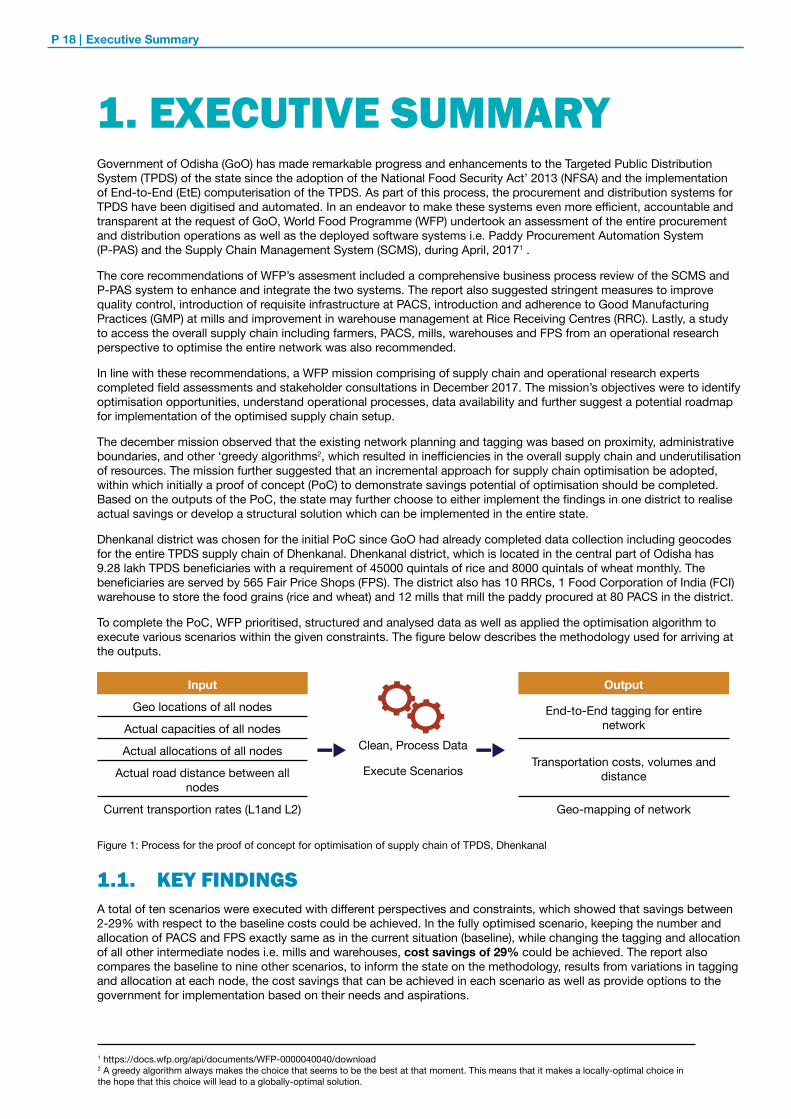
To complete the PoC, WFP prioritised, structured and analysed data as well as applied the optimisation algorithm to execute various scenarios within the given constraints. The figure below describes the methodology used for arriving at the outputs.
Input Output
Geo locations of all nodes
Clean, Process Data
Execute Scenarios
End-to-End tagging for entire networkActual capacities of all nodes
Actual allocations of all nodesTransportation costs, volumes and
distanceActual road distance between all nodes
Current transportion rates (L1and L2) Geo-mapping of network
Figure 1: Process for the proof of concept for optimisation of supply chain of TPDS, Dhenkanal
1.1. KEY FINDINGSA total of ten scenarios were executed with different perspectives and constraints, which showed that savings between 2-29% with respect to the baseline costs could be achieved. In the fully optimised scenario, keeping the number and allocation of PACS and FPS exactly same as in the current situation (baseline), while changing the tagging and allocation of all other intermediate nodes i.e. mills and warehouses, cost savings of 29% could be achieved. The report also compares the baseline to nine other scenarios, to inform the state on the methodology, results from variations in tagging and allocation at each node, the cost savings that can be achieved in each scenario as well as provide options to the government for implementation based on their needs and aspirations.
1 https://docs.wfp.org/api/documents/WFP-0000040040/download2 A greedy algorithm always makes the choice that seems to be the best at that moment. This means that it makes a locally-optimal choice in the hope that this choice will lead to a globally-optimal solution.
Executive Summary

Optimisation of TPDS Supply Chain | P 19
TOTAL COSTS AND SAVINGS : RS. 45,71,640
SCENARIO : BASELINE
GOAL: Model the existing network to calculate costs and prepare a base for comparison with other scenarios.
SCENARIO 1: BASELINE WITH CHANGE IN TRANSPORT PAYMENT MODALITY
GOAL: Investigate potential savings with change in transporter payment modality and rates from per Qtl. to per Qtl. per Km. in RRC to FPS transport.
KEY RESULT: Cost saving of 45% in the last leg i.e. from RRC to FPS.
TOTAL COSTS AND SAVINGS : RS. 36,95,980 (-19%)
SCENARIO 2: OPTIMISE PACS TAGGING
GOAL: Investigate potential savings by only changing the PACS tagging (assuming mill throughput is kept equal).
KEY RESULT: Tagging of 52 out of 80 PACS is changed resulting in average distance/Qtl. to decrease from 19.5 to 17.9 Km. in the leg 1 i.e. PACS to Mill.
TOTAL COSTS AND SAVINGS : RS. 44,84,219 (-2%)
(-6%)
SCENARIO 3: OPTIMISE LEG 1 AND 2
GOAL: Investigate potential savings by changing the PACS to Mill and Mill to RRC tagging (assuming mill throughput can change as well).
KEY RESULT: Tagging of 56 out of 80 PACS is changed. Average distance/Qtl. decreased from 19.5 to 13.5 Km in the PACS to Mill leg and from 19.2 to 11.9 Km. in the Mill to RRC leg
TOTAL COSTS AND SAVINGS : RS. 40,63,924 (-11%)
(-16%)
(-45%)
(-29%)
Additionally, the analysis found that by changing just the payment modality for transportation from RRC to FPS, from the ‘per Qtl.’ to ‘per Qtl. per Km.’ and using the rates as in the Mill to RRC leg itself lead to a saving of 19% from the current costs. The savings potential clearly indicates the need to review and revise the existing operational practices and policies with respect to the supply chain system, in a bid to achieve cost savings which can be reutilised for further benefit of the beneficiaries. Summary of the changes in the network in each scenario and the savings that can be achieved are described below:
Can be changed Remains the same Can be closed

P 20 |
SCENARIO 6: CLOSING PACS
GOAL: Investigate what PACS should be closed in order to minimise transportation costs, assuming that all PACS are able to supply their maximum capacity.
KEY RESULT: 12 out of 80 PACS are closed resulting in an average distance/Qtl. decrease from 19.5 km. to 13.6 Km. in the PACS to Mill leg.
TOTAL COSTS AND SAVINGS : RS. 43,23,411 (-5%)
(-15%)
SCENARIO 4: OPTIMISE FPS TAGGING
GOAL: Investigate potential savings by only changing the FPS tagging (assuming the transport rate in the last leg is changed from the ‘per Qtl.’ to ‘per Qtl. per Km’).
KEY RESULT: Tagging of 356 out of 565 FPS is changed which results in a decrease in average distance/Qtl. from 22.4 to 18.1 Km. in the RRC to FPS leg.
TOTAL COSTS AND SAVINGS : RS. 41,80,933 (-9%)
(-19%)
SCENARIO 5: CLOSING MILLS
GOAL: Investigate what mills should be used in order to minimise transportation costs assuming that all mills should either use their full capacity or be closed.
KEY RESULT: 6 out of 12 mills are closed, the average distance/Qtl has reduced from 19.5 Km. to 15.13 Km. in PACS to Mill leg and from 19.24 Km. to 15.78 Km. in Mill to RRC leg.
TOTAL COSTS AND SAVINGS : RS. 42,92,075 (-6%)
(-6%) (-14%)
SCENARIO 7: CLOSING FPS
GOAL: Investigate the effect on the transportation costs as the optimiser chooses to close the small FPS (<35 Qtl.) and shift their demand to another FPS that is close by (within 2 Km.).
KEY RESULT: 59 out of 565 FPS are closed resulting in a decrease in average distance/Qtl. from 21.67 km. to 17.34 km for the RRC to FPS leg.
TOTAL COSTS AND SAVINGS : RS.41,79,980 (-9%)
(-19%)
Executive Summary
Can be changed Remains the same Can be closed

Optimisation of TPDS Supply Chain | P 21
SCENARIO 9: FULLY OPTIMISED WITH CAPACITY CONSTRAINED +15%
GOAL: Investigate how much savings can be achieved by changing the tagging and assuming that each location in the network (mills and RRCs) can handle up to 15% more than the current throughput.
KEY RESULT: Centrally located mills and RRCs are being used more heavily resulting in an average distance/Qtl. decrease by 9%, 27% and 29% respectively in the three legs.
TOTAL COSTS AND SAVINGS : RS. 36,06,288 (-21%)
(-29%)(-27%)(-9%)
SCENARIO 8: FULLY OPTIMISED WITH CAPACITY CONSTRAINED
GOAL: Investigate how much savings can be achieved in the transportation cost by chnaging the tagging of all the nodes and assuming that the throughput of all locations (RRCs and mills) remain the same.
KEY RESULT: Tagging of 52 out of 80 PACS and 356 out of 565 FPS is changed. This results in an average distance/Qtl. decreases by 6%, 17% and 19% respectively in the three legs.
TOTAL COSTS AND SAVINGS : RS. 39,37,544 (-14%)
(-19%)(-17%)(-6%)
SCENARIO 10: FULLY OPTIMISED
GOAL: Investigate how much savings are possible by allowing the tagging and throughput of every location in the network to change (mills should not exceed capacity)
KEY RESULT: The throughput volume of almost all locations is changed resulting in an average distance/Qtl. decrease of 14%, 50% and 33% respectively in the three legs.
TOTAL COSTS AND SAVINGS : RS. 32,48,206 (-29%)
(-14%) (-50%) (-33%)
Table 1: Summary of scenarios and results
Can be changed Remains the same Can be closed

P 22 | Executive Summary

Optimisation of TPDS Supply Chain | P 23
2CHAPTER
INTRODUCTION
P 24 |
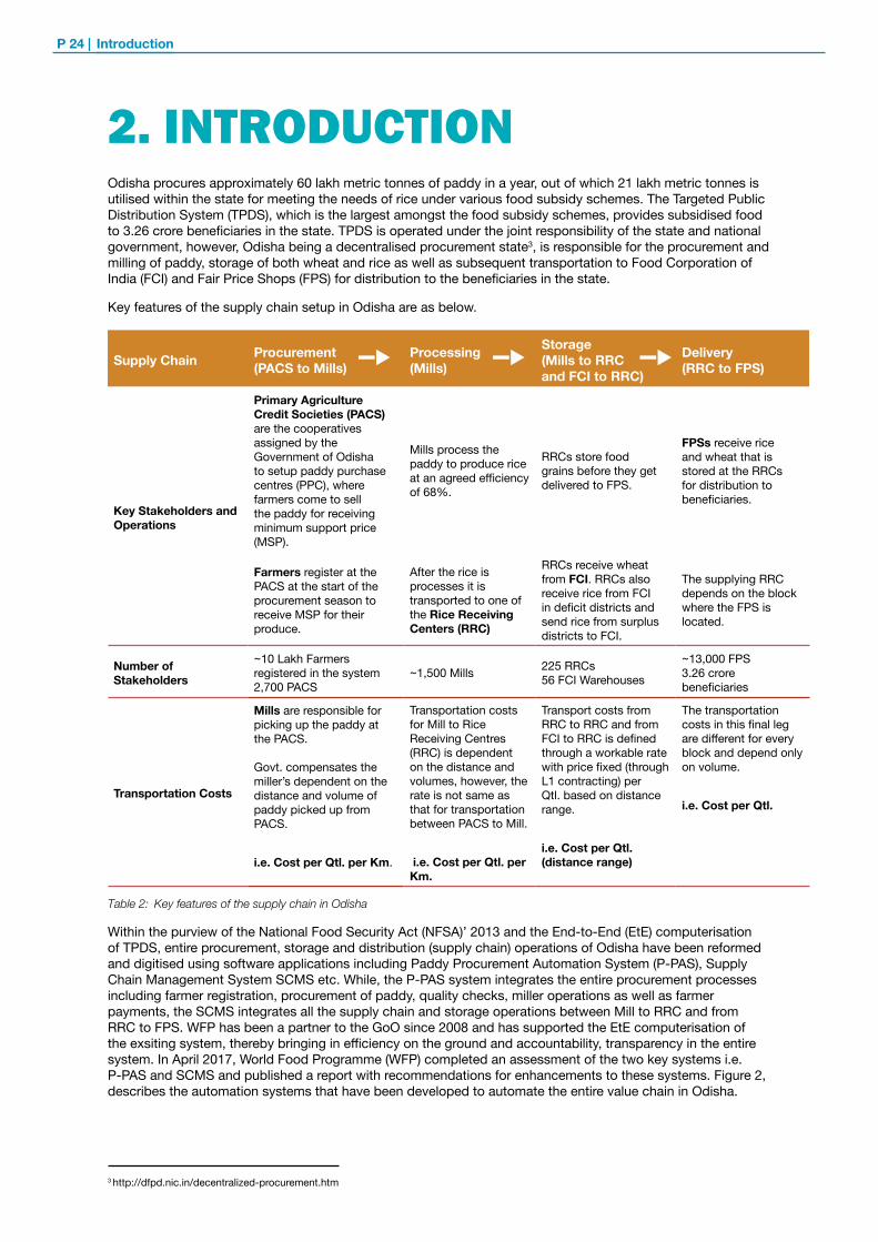
CHAPTER3. 2. INTRODUCTIONOdisha procures approximately 60 lakh metric tonnes of paddy in a year, out of which 21 lakh metric tonnes is utilised within the state for meeting the needs of rice under various food subsidy schemes. The Targeted Public Distribution System (TPDS), which is the largest amongst the food subsidy schemes, provides subsidised food to 3.26 crore beneficiaries in the state. TPDS is operated under the joint responsibility of the state and national government, however, Odisha being a decentralised procurement state3, is responsible for the procurement and milling of paddy, storage of both wheat and rice as well as subsequent transportation to Food Corporation of India (FCI) and Fair Price Shops (FPS) for distribution to the beneficiaries in the state.
Key features of the supply chain setup in Odisha are as below.
Supply Chain Procurement (PACS to Mills)
Processing (Mills)
Storage (Mills to RRC and FCI to RRC)
Delivery (RRC to FPS)
Key Stakeholders and Operations
Primary Agriculture Credit Societies (PACS) are the cooperatives assigned by the Government of Odisha to setup paddy purchase centres (PPC), where farmers come to sell the paddy for receiving minimum support price (MSP).
Mills process the paddy to produce rice at an agreed efficiency of 68%.
RRCs store food grains before they get delivered to FPS.
FPSs receive rice and wheat that is stored at the RRCs for distribution to beneficiaries.
Farmers register at the PACS at the start of the procurement season to receive MSP for their produce.
After the rice is processes it is transported to one of the Rice Receiving Centers (RRC)
RRCs receive wheat from FCI. RRCs also receive rice from FCI in deficit districts and send rice from surplus districts to FCI.
The supplying RRC depends on the block where the FPS is located.
Number of Stakeholders
~10 Lakh Farmers registered in the system 2,700 PACS
~1,500 Mills 225 RRCs 56 FCI Warehouses
~13,000 FPS 3.26 crore beneficiaries
Transportation Costs
Mills are responsible for picking up the paddy at the PACS. Govt. compensates the miller’s dependent on the distance and volume of paddy picked up from PACS.
i.e. Cost per Qtl. per Km.
Transportation costs for Mill to Rice Receiving Centres (RRC) is dependent on the distance and volumes, however, the rate is not same as that for transportation between PACS to Mill.
i.e. Cost per Qtl. per Km.
Transport costs from RRC to RRC and from FCI to RRC is defined through a workable rate with price fixed (through L1 contracting) per Qtl. based on distance range.
i.e. Cost per Qtl. (distance range)
The transportation costs in this final leg are different for every block and depend only on volume.
i.e. Cost per Qtl.
Table 2: Key features of the supply chain in Odisha
Within the purview of the National Food Security Act (NFSA)’ 2013 and the End-to-End (EtE) computerisation of TPDS, entire procurement, storage and distribution (supply chain) operations of Odisha have been reformed and digitised using software applications including Paddy Procurement Automation System (P-PAS), Supply Chain Management System SCMS etc. While, the P-PAS system integrates the entire procurement processes including farmer registration, procurement of paddy, quality checks, miller operations as well as farmer payments, the SCMS integrates all the supply chain and storage operations between Mill to RRC and from RRC to FPS. WFP has been a partner to the GoO since 2008 and has supported the EtE computerisation of the exsiting system, thereby bringing in efficiency on the ground and accountability, transparency in the entire system. In April 2017, World Food Programme (WFP) completed an assessment of the two key systems i.e. P-PAS and SCMS and published a report with recommendations for enhancements to these systems. Figure 2, describes the automation systems that have been developed to automate the entire value chain in Odisha.
3 http://dfpd.nic.in/decentralized-procurement.htm
Introduction

Optimisation of TPDS Supply Chain | P 25
The core recommendations of the April mission included a comprehensive business process review of the SCMS and P-PAS system to enhance and integrate the two systems. The report also suggested stringent measures to improve quality control, introduction of requisite infrastructure at PACS, introduction and adherence to Good Manufacturing Practices (GMP) at mills and improvement in warehouse management at RRCs to optimise the entire network was also recommended.Following up on the recommendation of the assessment from April 2017 and on the request of the Government of Odisha(GoO), a Supply Chain Optimisation (SCO) mission to Odisha took place in December 2017 to study optimisation opportunities from an operational research perspective in the supply chain for TPDS in Odisha.
2.1. KEY OBJECTIVESBased on the SCO scoping mission in December and in consultation with the government it was proposed to undertake a Proof of Concept (PoC) to identify the optimal network tagging for the supply chain network of the TPDS system for one district. The PoC was established by applying WFP’s optimisation approach and tools, leading to efficiency gains in the delivery of food grains and realisation of potential savings. Odisha’s Dhenkanal district, which has 9,28,884 TPDS beneficiaries and a total demand of 45,000 Qtls. of rice per month, was chosen for this assessment because of good data availability on account of an unrelated supply chain mapping exercise that was performed for this district.
The main goal of the SCO mission was to showcase that savings in comparison to the ‘as-is’ scenario, which can be achieved within an individual district. Since the supply chain setup in other districts is similar, it is very likely that these savings can then also be achieved in the other districts with similar supply chain setup.
The key objectives for the SCO mission were as below:
1. Mapping optimal network tagging and flow from PACS to FPS – Propose alternative and more efficient network allocation/tagging scenarios between different nodes of the supply chain (i.e. PACS to Mill, Mill to RRC etc.).
2. Clustering final delivery nodes by “Supply Zone” (and not by administrative block) – Suggest a new clustering of FPSs by supply zone (following the optimal allocation and not the geographical block structure) so that transportation in leg 3 i.e RRC to FPS can be optimised.
3. Estimate the potential/quantum of savings feasible under various scenarios.4. Verify the feasibility of results on ground.
Figure 2: Status of automation in the entire supply chain of Odisha
10 LakhsFarmers
2700Procurement
Centres
1500 Rice Mills
225Warehouses
Warehouses
Wheat
Mak
e on
-gro
und
activ
ities
effi
cien
t
On-
grou
nd a
ctiv
ities
au
tom
ated
Grievance Redressal System
Basic System for reporting
12,650FPS
6 Million MT Paddy
Farmer Registration
Module
Mobile apps for Millers
Paddy ProcurementAutomation system
Supply Chain Management System
Point of Sale Devices
Beneficiary Management
20 Lakhs (MT) tonnes
Rice and Wheat
3.4 croresTPDS
Beneficiaries
(All numbers mentioned above are approx.)
P 26 |
2.2. APPROACH AND METHODOLOGY The initial scoping mission in December was completed to conduct interviews with key stakeholders, visit field operations and to collect and screen documents and data. The data and information collected was further analysed to identify and prioritise potential areas of optimisation. The scoping mission also accessed feasibility, potential next steps and charted a roadmap for project implementation. An initial assessment of Dhenkanal district which was identified for the PoC was completed and showed that:
• Data was captured and available for all nodes of the supply chain.• Supply chain network was sufficiently complex and based on ‘greedy algorithms’ to merit the use of
optimisation software to support planning. • There were opportunities to apply optimisation algorithms to existing data to identify a more efficient and
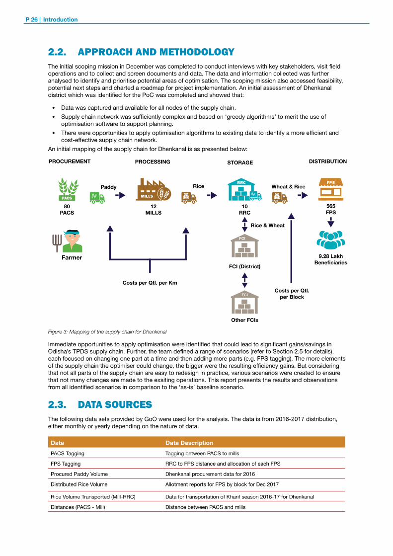
cost-effective supply chain network.An initial mapping of the supply chain for Dhenkanal is as presented below:
Figure 3: Mapping of the supply chain for Dhenkenal
Immediate opportunities to apply optimisation were identified that could lead to significant gains/savings in Odisha’s TPDS supply chain. Further, the team defined a range of scenarios (refer to Section 2.5 for details), each focused on changing one part at a time and then adding more parts (e.g. FPS tagging). The more elements of the supply chain the optimiser could change, the bigger were the resulting efficiency gains. But considering that not all parts of the supply chain are easy to redesign in practice, various scenarios were created to ensure that not many changes are made to the exsiting operations. This report presents the results and observations from all identified scenarios in comparison to the ‘as-is’ baseline scenario.
2.3. DATA SOURCES The following data sets provided by GoO were used for the analysis. The data is from 2016-2017 distribution, either monthly or yearly depending on the nature of data.
Data Data DescriptionPACS Tagging Tagging between PACS to mills
FPS Tagging RRC to FPS distance and allocation of each FPS
Procured Paddy Volume Dhenkanal procurement data for 2016
Distributed Rice Volume Allotment reports for FPS by block for Dec 2017
Rice Volume Transported (Mill-RRC) Data for transportation of Kharif season 2016-17 for Dhenkanal
Distances (PACS - Mill) Distance between PACS and mills
Introduction
Other FCIs
FCI (District)
PROCUREMENT PROCESSING STORAGE DISTRIBUTION
Costs per Qtl. per KmCosts per Qtl.
per Block
9.28 Lakh Beneficiaries
Rice & Wheat
80PACS
12MILLS
10 RRC
565FPS
Farmer
Paddy Rice Wheat & Rice
Optimisation of TPDS Supply Chain | P 27
Data Data DescriptionDistances (Mill - RRC) Distance between mills and RRCs
Distances (RRC - FPS) Distance between RRCs and FPSs
Distances (FCI - RRC) Distance between FCI warehouse and RRCs
Transport rates (PACS – Mill / Mill - RRC) Transportation rates for PACS to mills and mills to RRCs
Transport rates (RRC - FPS) Transportation rates for RRCs to FPSs
PACS locations and capacities Latitude, longitude and capacity details of PACS
Mill locations Latitude and longitude of the mills
Mill capacities Mill allocation and capacity details
RRC locations Latitude and longitude of RRCs in Dhenkanal
RRC capacities Storage capacity of RRCs in Qtls.
FPS locations Latitude and longitude details for FPSs
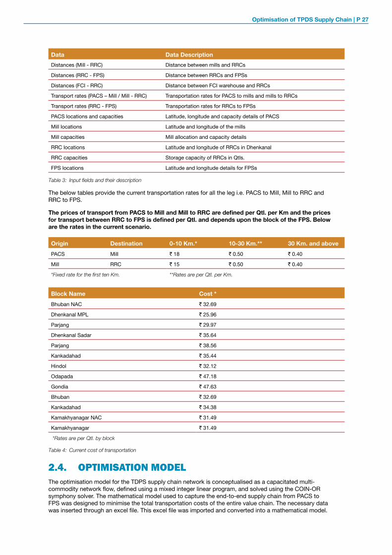
Table 3: Input fields and their description
The below tables provide the current transportation rates for all the leg i.e. PACS to Mill, Mill to RRC and RRC to FPS.
The prices of transport from PACS to Mill and Mill to RRC are defined per Qtl. per Km and the prices for transport between RRC to FPS is defined per Qtl. and depends upon the block of the FPS. Below are the rates in the current scenario.
Origin Destination 0-10 Km.* 10-30 Km.** 30 Km. and abovePACS Mill ` 18 ` 0.50 ` 0.40
Mill RRC ` 15 ` 0.50 ` 0.40
*Fixed rate for the first ten Km. **Rates are per Qtl. per Km.
Block Name Cost *Bhuban NAC ` 32.69
Dhenkanal MPL ` 25.96
Parjang ` 29.97
Dhenkanal Sadar ` 35.64
Parjang ` 38.56
Kankadahad ` 35.44
Hindol ` 32.12
Odapada ` 47.18
Gondia ` 47.63
Bhuban ` 32.69
Kankadahad ` 34.38
Kamakhyanagar NAC ` 31.49
Kamakhyanagar ` 31.49
*Rates are per Qtl. by block
Table 4: Current cost of transportation
2.4. OPTIMISATION MODELThe optimisation model for the TDPS supply chain network is conceptualised as a capacitated multi-commodity network flow, defined using a mixed integer linear program, and solved using the COIN-OR symphony solver. The mathematical model used to capture the end-to-end supply chain from PACS to FPS was designed to minimise the total transportation costs of the entire value chain. The necessary data was inserted through an excel file. This excel file was imported and converted into a mathematical model.
P 28 |
This method ensured that it would be easy to re-run the model in case the data changed and that it would also be possible to run the same model for a different district if the data is available in a structured format. Depending on the scenario, a (slightly) different mathematical optimisation model was solved to identify the optimal solution for the corresponding scenario.
• A solution consists of the allocation of volume (rice, wheat and paddy) that should travel between all locations (e.g. PACS to Mill, RRC to FPS, etc.) to minimise the total transportation costs.
• The script further generates three different outputs for the specific scenario:
‣ A table containing the Key Performance Indicators (KPIs) such as transportation cost, average costs and average distance travelled for all the legs in the supply chain network.
‣ A file containing the details of the cost or transportation, distance and volume of commodity (rice/wheat/paddy) travelled between each node (e.g. between each mill to each RRC) of the supply chain network.
‣ Maps that visualise the supply chain network and the tagging of various locations (e.g. RRC to FPS) using geocodes.
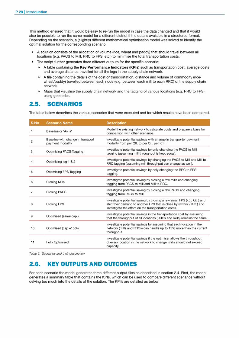
2.5. SCENARIOSThe table below describes the various scenarios that were executed and for which results have been compared.
S.No Scenario Name Description
1 Baseline or ‘As is’ Model the existing network to calculate costs and prepare a base for comparison with other scenarios.
2 Baseline with change in transport payment modality
Investigate potential savings with change in transporter payment modality from per Qtl. to per Qtl. per Km.
3 Optimising PACS Tagging Investigate potential savings by only changing the PACS to Mill tagging (assuming mill throughput is kept equal).
4 Optimising leg 1 & 2 Investigate potential savings by changing the PACS to Mill and Mill to RRC tagging (assuming mill throughput can change as well).
5 Optimising FPS Tagging Investigate potential savings by only changing the RRC to FPS tagging.
6 Closing Mills Investigate potential saving by closing a few mills and changing tagging from PACS to Mill and Mill to RRC.
7 Closing PACS Investigate potential saving by closing a few PACS and changing tagging from PACS to Mill.
8 Closing FPSInvestigate potential saving by closing a few small FPS (<35 Qtl.) and shift their demand to another FPS that is close by (within 2 Km.) and investigate the effect on the transportation costs.
9 Optimised (same cap.) Investigate potential savings in the transportation cost by assuming that the throughput of all locations (RRCs and mills) remains the same.
10 Optimised (cap +15%)Investigate potential savings by assuming that each location in the network (mills and RRCs) can handle up to 15% more than the current throughput.
11 Fully OptimisedInvestigate potential savings if the optimiser allows the throughput of every location in the network to change (mills should not exceed capacity).
Table 5: Scenarios and their description
2.6. KEY OUTPUTS AND OUTCOMESFor each scenario the model generates three different output files as described in section 2.4. First, the model generates a summary table that contains the KPIs, which can be used to compare different scenarios without delving too much into the details of the solution. The KPI’s are detailed as below:
Introduction

Optimisation of TPDS Supply Chain | P 29
KPI: Unit: Description:
1. Total Transportation Costs: Rs.The total costs that are incurred for transportation. Calculated separately for the transport of paddy, rice and wheat and for every transportation leg.
2. Average Transportation Costs: Rs. / Km. / Qtl.
The average transportation costs are calculated per Km. per Qtl. This allows a comparison of costs incurred in the different transportation legs.
3. Average Distance Travelled4: Km./Qtl.
This KPI indicates the average distance that each Qtl. of grain has to travel to get from its origin to its destination in the corresponding transportation leg.
Table 6: Key output KPI’s and their description
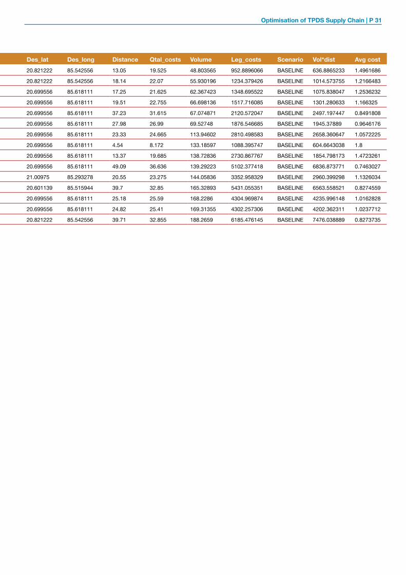
Secondly, the model generates an excel file that contains details for every location and supply chain leg in the optimised configuration of the network for every scenario segregated by type of commodity (refer table 7 on next page). For each movement the optimiser captures the origin and destination locations, the volume transported, commodity type, distance travelled, and the average and total transportation costs that are incurred. This file can be used to analyse the optimal network configuration in more detail and to aggregate the results. Finally, for every leg in the transportation network, the model generates maps that help visualise the supply chain network and the tagging of various locations (e.g. RRC – FPS) using geocodes (refer figure 4).
These results can be used to gain valuable insights on how to achieve savings on transportation cost. Insights from various scenarios could inform a policy, operational or technical change in the supply chain configuration. Below are some of outputs from the models which can inform operational, technical or policy level changes.
TAGGING AND DISTANCE
• Tagging of PACS to Mill and Mill to RRC.• Tagging between FCI to RRC and RRC to FPS.• Distance travelled between PACS to Mill, Mill to RRC, FCI to RRC and from RRC to FPS.
VOLUME
• Volume of paddy supplied between each PACS and mill.• Volume of rice supplied by each mill to each RRC and wheat from FCI to each RRC.• Volume from each RRC to each FPS without any change in the total allocation for each FPS.
COSTS
• Ideal transport rate which should be negotiated for the RRC to FPS transport leg.
4 Distance travelled for wheat to reach FCI godowns in Odisha is not included
Figure 4: Sample output map of PACS to Mills in baseline
BaselinePACS-MILL

P 30 |
2.7. LIMITATIONS OF THE MODEL AND ANALYSISThis PoC focused on mapping the supply chain network and analysing the grain flow between various locations, however even while it provides details of the tagging, volume, distance and costs of transportation between various legs, there are a few limitations to this model, which are detailed as below:
1. The model does not consider the time dimension (e.g. months, weeks) and therefore it cannot be used to answer questions that relate to time (e.g. when to purchase paddy at PACS; how long to store rice at RRCs; when to dispatch a truck from Mill to RRC).
2. The model focuses exclusively on minimising transport costs, so it does not account for costs related to processing at RRCs i.e. storage, loading and unloading costs, etc., since they increase or decrease depending on the change in volume.
3. The PoC focused on a single district, which means the current model does not look at inter-district flows (e.g. sending surplus rice to an FCI, supplying an FPS from a RRC in a different district, etc.) hence:
‣ Absolute savings that can be achieved through optimisation is not very large.
‣ Efficiency gains by dropping the administrative boundaries of the district itself could not be defined i.e. more efficiencies can be realised once the entire supply chain is optimised.
Note: For future applications these limitations can be addressed by improving the model, assuming the required data is made available.
Introduction
Table 7: Sample output -excel file PACS to Mills in baseline
Leg Origin Destination Commodity Block Ori_lat Ori_long Des_lat Des_long Distance Qtal_costs Volume Leg_costs Scenario Vol*dist Avg cost PACS-MILL S1090506 NATURAL AGRITECH PVT LTD PADDY KAMAKHYANAGAR 20.912028 85.518111 20.821222 85.542556 13.05 19.525 48.803565 952.8896066 BASELINE 636.8865233 1.4961686
PACS-MILL S1090702 NATURAL AGRITECH PVT LTD PADDY ODAPADA 20.706722 85.510806 20.821222 85.542556 18.14 22.07 55.930196 1234.379426 BASELINE 1014.573755 1.2166483
PACS-MILL S1090210 BDN FOOD PRODUCTS PADDY DHENKANAL 20.571472 85.63125 20.699556 85.618111 17.25 21.625 62.367423 1348.695522 BASELINE 1075.838047 1.2536232
PACS-MILL S1090307 BDN FOOD PRODUCTS PADDY GANDIA 20.786444 85.7225 20.699556 85.618111 19.51 22.755 66.698136 1517.716085 BASELINE 1301.280633 1.166325
PACS-MILL S1090310 BDN FOOD PRODUCTS PADDY GANDIA 20.846 85.856028 20.699556 85.618111 37.23 31.615 67.074871 2120.572047 BASELINE 2497.197447 0.8491808
PACS-MILL S1090312 BDN FOOD PRODUCTS PADDY GANDIA 20.850306 85.748278 20.699556 85.618111 27.98 26.99 69.52748 1876.546685 BASELINE 1945.37889 0.9646176
PACS-MILL S1090306 BDN FOOD PRODUCTS PADDY GANDIA 20.741111 85.783667 20.699556 85.618111 23.33 24.665 113.94602 2810.498583 BASELINE 2658.360647 1.0572225
PACS-MILL S1090201 BDN FOOD PRODUCTS PADDY DHENKANAL 20.725806 85.60075 20.699556 85.618111 4.54 8.172 133.18597 1088.395747 BASELINE 604.6643038 1.8
PACS-MILL S1090208 BDN FOOD PRODUCTS PADDY DHENKAMAL 20.786083 85.636528 20.699556 85.618111 13.37 19.685 138.72836 2730.867767 BASELINE 1854.798173 1.4723261
PACS-MILL S1090314 BDN FOOD PRODUCTS PADDY GANDIA 20.796972 85.992417 20.699556 85.618111 49.09 36.636 139.29223 5102.377418 BASELINE 6836.873771 0.7463027
PACS-MILL S1090801 BHUTIA FOOD PVT LTD PADDY PARAJANG 20.942389 85.417167 21.00975 85.293278 20.55 23.275 144.05836 3352.958329 BASELINE 2960.399298 1.1326034
PACS-MILL S1090303 HARAPRIYA RICE MILL PADDY GANDIA 20.790278 85.761 20.601139 85.515944 39.7 32.85 165.32893 5431.055351 BASELINE 6563.558521 0.8274559
PACS-MILL S1090303 BDN FOOD PRODUCTS PADDY GANDIA 20.790278 85.761 20.699556 85.618111 25.18 25.59 168.2286 4304.969874 BASELINE 4235.996148 1.0162828
PACS-MILL S1090202 BDN FOOD PRODUCTS PADDY DHENKANAL 20.618278 85.642472 20.699556 85.618111 24.82 25.41 169.31355 4302.257306 BASELINE 4202.362311 1.0237712
PACS-MILL S1090303 NATUAL AGRITECH PVT LTD PADDY GANDIA 20.790278 85.761 20.821222 85.542556 39.71 32.855 188.2659 6185.476145 BASELINE 7476.038889 0.8273735
Optimisation of TPDS Supply Chain | P 31
Leg Origin Destination Commodity Block Ori_lat Ori_long Des_lat Des_long Distance Qtal_costs Volume Leg_costs Scenario Vol*dist Avg cost PACS-MILL S1090506 NATURAL AGRITECH PVT LTD PADDY KAMAKHYANAGAR 20.912028 85.518111 20.821222 85.542556 13.05 19.525 48.803565 952.8896066 BASELINE 636.8865233 1.4961686
PACS-MILL S1090702 NATURAL AGRITECH PVT LTD PADDY ODAPADA 20.706722 85.510806 20.821222 85.542556 18.14 22.07 55.930196 1234.379426 BASELINE 1014.573755 1.2166483
PACS-MILL S1090210 BDN FOOD PRODUCTS PADDY DHENKANAL 20.571472 85.63125 20.699556 85.618111 17.25 21.625 62.367423 1348.695522 BASELINE 1075.838047 1.2536232
PACS-MILL S1090307 BDN FOOD PRODUCTS PADDY GANDIA 20.786444 85.7225 20.699556 85.618111 19.51 22.755 66.698136 1517.716085 BASELINE 1301.280633 1.166325
PACS-MILL S1090310 BDN FOOD PRODUCTS PADDY GANDIA 20.846 85.856028 20.699556 85.618111 37.23 31.615 67.074871 2120.572047 BASELINE 2497.197447 0.8491808
PACS-MILL S1090312 BDN FOOD PRODUCTS PADDY GANDIA 20.850306 85.748278 20.699556 85.618111 27.98 26.99 69.52748 1876.546685 BASELINE 1945.37889 0.9646176
PACS-MILL S1090306 BDN FOOD PRODUCTS PADDY GANDIA 20.741111 85.783667 20.699556 85.618111 23.33 24.665 113.94602 2810.498583 BASELINE 2658.360647 1.0572225
PACS-MILL S1090201 BDN FOOD PRODUCTS PADDY DHENKANAL 20.725806 85.60075 20.699556 85.618111 4.54 8.172 133.18597 1088.395747 BASELINE 604.6643038 1.8
PACS-MILL S1090208 BDN FOOD PRODUCTS PADDY DHENKAMAL 20.786083 85.636528 20.699556 85.618111 13.37 19.685 138.72836 2730.867767 BASELINE 1854.798173 1.4723261
PACS-MILL S1090314 BDN FOOD PRODUCTS PADDY GANDIA 20.796972 85.992417 20.699556 85.618111 49.09 36.636 139.29223 5102.377418 BASELINE 6836.873771 0.7463027
PACS-MILL S1090801 BHUTIA FOOD PVT LTD PADDY PARAJANG 20.942389 85.417167 21.00975 85.293278 20.55 23.275 144.05836 3352.958329 BASELINE 2960.399298 1.1326034
PACS-MILL S1090303 HARAPRIYA RICE MILL PADDY GANDIA 20.790278 85.761 20.601139 85.515944 39.7 32.85 165.32893 5431.055351 BASELINE 6563.558521 0.8274559
PACS-MILL S1090303 BDN FOOD PRODUCTS PADDY GANDIA 20.790278 85.761 20.699556 85.618111 25.18 25.59 168.2286 4304.969874 BASELINE 4235.996148 1.0162828
PACS-MILL S1090202 BDN FOOD PRODUCTS PADDY DHENKANAL 20.618278 85.642472 20.699556 85.618111 24.82 25.41 169.31355 4302.257306 BASELINE 4202.362311 1.0237712
PACS-MILL S1090303 NATUAL AGRITECH PVT LTD PADDY GANDIA 20.790278 85.761 20.821222 85.542556 39.71 32.855 188.2659 6185.476145 BASELINE 7476.038889 0.8273735
P 32 | Introduction

Optimisation of TPDS Supply Chain | P 33
3BASELINE
CHAPTER

P 34 |
3.1. ABOUT THE SCENARIOThe main purpose of this scenario is to model the current configuration of the procurement and distribution network of Dhenkanal district and quantify the exsiting tagging, volumes and cost of transportation. The baseline is vital to validate model assumptions, inputs, and outputs, and enable comparison of other optimised scenarios against the performance of the current supply chain setup. The outputs under this scenario have been generated based on actual data from the existing supply chain setup.
SCENARIO: BASELINE
**TTC - Total Transport Costs | ADT - Average Distance Travelled | ATC - Average Transportation Costs
TTC: Rs. 45,71,640 | ADT: 84 Km./Qtl. | ATC: 1.21 Rs. per Km./Qtl.
Furthermore, this scenario has also been used to calculate the estimated transport rate (per Qtl. Per Km.) for the last leg (RRC-FPS) based on the existing cost of transportation, which is paid out to the transporters. The estimated cost is then further used to show potential savings in other scenarios. Please find below the table described the cost calculations.
3.2. KEY CONSTRIANTS1. Every PACS can only supply a mill that it’s connected to according to the current PACS tagging.2. All paddy that is procured is transported to one of the mills in the district.3. All paddy that is procured from the PACS is processed by the mills.4. All mills have an efficiency of 68%: for every Kg. of paddy that flows into the mill it produces exactly
0.68 Kg. of rice.5. The volumes of rice that are being transported from mills to RRCs are given by the data.6. All rice that is produced at the mills is transported to one of the 10 RRCs in Dhenkanal.7. FPS can only be supplied by a RRC that it’s connected to according to the current FPS tagging (this holds
for the supply of both rice and wheat). 8. All demand for rice and wheat at every FPS must be satisfied.9. The wheat allocation of every RRC is defined by the wheat demand of the connected FPSs.10. All wheat demand in the district is fulfilled from FCI (Dhenkanal). 11. Rice delivered from RRC to FPS is as per the FPS allocation, any remaining quantity of rice is stored for
further use or transport to deficit districts.
Table 8: Key statistics for the baseline
BASELINE
Baseline
5 Values are rounded off to maximum two decimal places, hence there may be slight differences in computed transportation costs as compared to the values provided.
Table 9: Calculation of estimated current transport rate per Qtl. per Km.
LEG
Rs. 19,34,274.29 Rs. 11,85,592.69 Rs. 1.63
Total Transportation Costs (Rs. /month)
(A)
Sum of Volume*Distance (Rs. /Qtl. /km)
(B)
Average Cost (Rs. /Qtl./ Km)
(C=A/B)
Can be changed Remains the same Can be closed

Optimisation of TPDS Supply Chain | P 35
3.3. SUMMARY STATISTICS
80
Number of RRCs (Rice)
73,529 Qtls.
Quantity Stored at RRC (Rice)
12
Number of FPS (Rice)
50,000 Qtls.
Quantity Delivered at FPS
(Rice)
10
Number of FPS (Wheat)
8000 Qtls.
Quantity Delivered at FPS
(Wheat)
Baseline 15,69,794 (34%) 1.09 19.51
Total Transportation Costs (Rs. /month):
Average Transportation Costs (Rs. /Qtl. /Km.):
Average Distance Travelled (Km. /Qtl.):
Baseline 0.95 19.249,09,631 (20%)
Baseline 1.63 22.4016,44,524 (36%)
Baseline 1.63 22.222,89,750 (6%)
Table 10: Summary statistics for the baseline
Baseline 1,57,941 (4%) 0.86 22.92
Wheat (8000 Qtls.)
Wheat (8000 Qtls.)
Rice (45,000 Qtls)
Rice (45,000 Qtls)
Paddy (73,529 Qtls)
Baseline:
Baseline:
Table 11: Key outputs for the baseline
3.4. KEY PERFORMANCE INDICATORS
Parameters:
Parameters:
Number of PACS
Quantity Procured at
PACS (Paddy)
Number of Mills
Output Quantity of Mills (Rice)
Number of RRCs (Wheat)
Quantity Stored at RRC
(Wheat)
10 50,000 Qtls. 565 45000 Qtls. 565 8000 Qtls.
Figure 5: Total distance and cost of transportation by leg for the baseline 5
Baseline
Cos
t of t
rans
port
atio
n ( i
n R
s. L
akh
)
Aver
age
Dis
tace
/Qtl.
PACS-MILL
Paddy Rice Wheat
PACS-MILLMILL-RRC MILL-RRCFCI-RRC FCI-RRCRRC-FPS RRC-FPSRRC-FPS RRC-FPS
15.7
9.1
1.58
16.4519.51 19.24 22.92 22.40 22.22
2.9

P 36 |
The figure 5, shows the breakup of transportation costs per leg in comparison to the average distance travelled per Qtl. For Leg 1, 2, 3, the costs are derived per Qtl. per Km. and for Leg 4 the costs are by Qtl., but restricted to a block. As can be observed, maximum cost is incurred in Leg 4 followed by Leg 1.
3.4.1. OBSERVATIONS FOR LEG 1: PACS TO MILL
3.4.1.1. TAGGING AND VOLUME
• There are 80 PACS and 12 mills, while the nodes traversed are 125, which shows that many PACS are attached to each mill or vice versa (Figure 6).
• Even through there are 14 PACS tagged to Mill2 (BDN Food Products) the total paddy allocated to the mill is amongst the lowest in the district.
• Milling allocation is evenly distributed and all mills, except Mill 2 and Mill 11 have an average allocation of ~6500 Qtls.
3.4.1.2. DISTANCE AND COSTS
• The cost of transportation in Leg 1 and the average distance/Qtl travelled from PACS to Mill is described in figure 7. As can be observed, the average distance/Qtl travelled between PACS and Mill 2 (BDN Food Products) is above average (i.e 19.4), but the cost of transportation is amongst the lowest.
Baseline
Figure 6: Tagging and volume from PACS to mills in baseline
8,222
13
Mill1
2,630
14
Mill2
7,335
12
Mill3
5,983
10
Mill4
6,975
12
Mill5
7,314
10
Mill6
6,058
8
Mill7
7,212
10
Mill8
6,184
14
Mill9
6,754
11
Mill10
1,764
4
Mill11
7,097
7
Mill12
Cou
nt o
f PAC
S Ta
gged
to M
ills
Volu
me
of P
addy
(Qtls
.)
PACS-MILL
Figure 7: Distance and cost of transportation from PACS to Mill in baseline
2.0
0.5
1.71.1
1.7 1.5 1.2 1.21.6 1.6
0.41.3
PACS-MILL
Aver
age
Dis
tanc
e/Q
tl.C
ost o
f tra
nspo
rtat
ion
(in R
s. L
akh)
23.8520.05 21.93
14.63
22.9217.91 17.86
12.08
29.08
20.85 18.3613.83
Mill1 Mill2 Mill3 Mill4 Mill5 Mill6 Mill7 Mill8 Mill9 Mill10 Mill11 Mill12

Optimisation of TPDS Supply Chain | P 37
• In line with the above observation, figure 8 describes the volume and cost of transportation for Mill 1(Annapurna Rice Mill), which has the highest cost of transportation and Mill 2 (BDN Food Products), which has one of the least costs of transportation. The results indicate that the cost of transporting paddy in distance range of 0-10 km is much lower than in any other distance range. For Mill 2 (BDN Food Products), 46% of the paddy is being delivered by PACS within 0-10 km distance range while incurring only 23% of the costs. This indicates a potential to maximise tagging within this distance range to minimise costs.
3.4.2. OBSERVATIONS FOR LEG 2: MILL TO RRC, FCI TO RRC
3.4.2.1. TAGGING AND VOLUME
• Total number of mills is 12, which are tagged to 10 RRCs, but the total number of nodes traversed from mills to RRC is 57 (Figure 9).
• Wheat is supplied from FCI Dhenkanal to all the 10 RRCs and hence the tagging is one to one.• Figure 9, also represents the volume of rice from mills to each RRC. It can be observed that even though
RRC 6 (Dhenkanal) and RRC10 (Mahispat (II)) are tagged to 8 and 7 mills respectively, the handled volume is amongst the lowest in the district.
3.4.2.2. DISTANCE AND COSTS
• Figure 10, describes the cost of transportation and average distance/Qtl between mills and RRCs and FCI to RRC.
• The distance for RRC 6 (Dhenkanal) in the FCI to RRC leg is zero because RRC 6 and FCI Dhenkanal located in the same place.
Figure 8: Volume and cost of transportation of paddy over distance range in baseline
1 11 11 1
24.19%
14.78%
<10KM
40.88%35.41%
10-20 KM
6.82% 7.31%
20-40 KM
28.11%
42.50%
40 KM>
46.47%
22.81%
<10 KM
10.18% 10.56%
10-20 KM
22.36%29.10%
20-40 KM
20.98%
37.53%
40 KM>
% of Total Cost% of Total Volume
Annapurana Rice Mill BDN Food Products
Volume of Paddy and Cost of Transportation
Figure 9: Tagging and volume of rice and wheat from mills and FCI respectively to RRC in baseline
5,207
11,040
4,450
2,144
5,020
2,0223,639
7,040 7,547
1,592 988 1,825502 399 789 1,086 364 1,106 589 351
5
10
3 4 4
85
2
9
1 1 1 1 1 1 1 1 1 1
7
MILL-RRC
RRC1 RRC2 RRC3 RRC4 RRC5 RRC6 RRC7 RRC8 RRC9 RRC10 RRC1 RRC2 RRC3 RRC4 RRC5 RRC6 RRC7 RRC8 RRC9 RRC10
FCI-RRC
Cou
nt o
f Mill
sta
gged
to R
RC
Volu
me
(Qlts
.)
Volu
me
(Qlts
.)C
ount
of F
CI w
areh
ouse
tagg
ed to
RR
C

P 38 |
3.4.3. OBSERVATIONS FOR LEG 3: RRC TO FPS
3.4.3.1. TAGGING AND VOLUME
RRC 2 and 9 i.e. Baladiabandha and Mahispat (I) handle one of the highest volume of rice from mills (11,040 and 7040 Qtls. respectively) and the distance travelled between Mill to RRC is also the highest as can be seen. in figure 11, hence the cost of transportation is the highest for these RRC’s in the Mill to RRC leg.
Baseline
Cos
t of t
rans
port
atio
n( i
n R
s. L
akh
)
Figure 10: Distance and cost of transportation from mills to RRCs and FCI to RRC in baseline
8
FCI-RRCMILL-RRC
Aver
age
Dis
tanc
e/Q
tl.C
ost o
f tra
nspo
rtat
ion
( in
Rs.
Lak
h )
Aver
age
Dis
tanc
e/Q
tl.
15.0
RRC2 RRC6RRC1
26.64
RRC2
28.55
RRC3
14.23
RRC4
13.38
RRC5
25.35
RRC6
27.29
RRC7
5.39
RRC8
5.97
RRC9
18.51
RRC10
17.64
RRC1
37.29
RRC3
41.48
RRC4
36.79
RRC5
49.03
RRC7
10.23
RRC8
30.50
RRC9
7.77
RRC10
7.81
1.1
2.7
0.80.3
1.10.5 0.3
0.6
1.4
0.3 0.3 0.3 0.2 0.1 0.30 0.1 0.3 0.1 0
Figure 11: Total Distance from Mills to RRC in baseline
RRC1
127
Tota
l Dis
tanc
e (K
m.)
RRC2
308
RRC3
47
RRC4
67
RRC5
126
RRC6
191
RRC7
67
RRC8
12
RRC9
199
RRC10
131
MILL-RRC
Figure 12: Tagging and volume of rice and wheat from RRC to FPS in baseline
RRC-FPS
RRC5
Cou
nt o
f Mill
sTa
gged
to R
RC
Volu
me
(Qtls
.)
RRC1
5,674
7448
RRC2
142
11,761
RRC3
51
4,777
RRC4
40
2,329
5,307
RRC6
74
2,9062,906
RRC7
43
3,639
RRC8
110
7,442
RRC9
105
7,381
RRC10
38
1,783

Optimisation of TPDS Supply Chain | P 39
The tagging and volume (rice and wheat) from RRCs to FPS in the baseline is represented in figure 12. The volume of food grains is dependent on the demand of the tagged FPS. The demand of each FPS is further dependent on the number of cards tagged to the FPS. As can be observed, RRC 2 (Baladiabandha) has the highest allocation and the most number of FPS tagged to it.
3.4.3.2. DISTANCE AND COSTS
Figure 13, describes the cost of transportation and distance travelled for delivering foodgrains from RRC to FPS. Cost of transportation is dependent only on the volume of foodgrains. s can be seen for RRC5 (Bhubhan) and RRC9 (Mahispat I), the average distance/Qtl. for paddy is much lower for RRC9 than RRC5, but since the volume of foodgrains at RRC9 is higher, the cost of transportation is also higher for RRC9.
3.4.4. GEOSPATIAL REPRESENTATION OF THE SUPPLY CHAIN NETWORK IN BASELINE
Figure 14: Geo-representation of tagging from PACS to Mill in baseline
Baseline
Mill 1 Mill 2 Mill 3 Mill 4 Mill 5 Mill 6 Mill 7 Mill 8 Mill 9 Mill 10 Mill 11 Mill 12
Destination
• Some of the cereals coming from nearby PACS need to move several kms. further to arrive to another miller, probably since the capacity of the closest miller is already filled.
• It can be observed from map in figure 14 that tagging of PACS is done miller by miller and there are significant overlaps in the map tagging from PACS to Mills, which shows a potential for optimisation.
• It can also be seen that most of the PACS are located on the east side of the district and a lot of paddy has to move from east to the west or central part of the district for milling. As an example, there are 12 PACS attached to Mill 3 (Bhutia Foods Pvt. Ltd.) which is in the north west of the district. Many of the PACS tagged to this mill are in the far east of the district. This type of tagging results in increased costs in this leg.
PACS-MILL
Figure 13: Distance and cost of transportation from RRC to FPS in baseline
RRC-FPS
Aver
age
Dis
tanc
e/Q
tl.C
ost o
f tra
nspo
tatio
n(in
Rs.
Lak
h )
RRC2 RRC3 RRC4 RRC5 RRC6 RRC7 RRC8 RRC9 RRC10RRC1
21.30
41.09
16.8412.46
25.3318.11
13.66 13.00 15.22 14.62
1.9
4.8
1.50.7
2.5
1.2 1.1
2.4 2.6
0.6

P 40 | Baseline
Figure 16: Geo-representation of tagging from FCI to RRC in baseline
Baseline
Figure 17: Geo-representation of tagging from RRC to FPS in baseline
Baseline
Map in figure 16 shows that the tagging from FCI to RRC is one to one and all RRC’s are tagged to the FCI for procuring wheat.
Figure 17, shows that RRCs in the south are even tagged to FPSs which are way up north. (Map is only representing movement of rice). As an example, RRC 2(Baladiabandha) which is in south of the district is tagged to FPSs in the extreme north, which could have been serviced by RRC 1 (Badasuanlo) and RRC 3 (Barihapur). Overall, tagging of RRCs to FPSs neither seems to follow a proximity approach nor block boundaries.
BaselineMILL-RRC
Figure 15: Geo-representation of tagging from Mill to RRC in baseline
Map shown in figure 15, describes the tagging between mills and RRCs. The tagging does not seem to follow the proximity approach. As an example, there are 10 mills attached to RRC 2 (Baladiabandha). These mills are much closer to other RRCs than RRC 10 (Mahispat II), which highlights opportunities in the network planning.
FCI-RRC
RRC-FPS
RRC 1 RRC 2 RRC 3 RRC 4 RRC 5 RRC 6 RRC 7 RRC 8 RRC 9 RRC 10
Destination
RRC 1 RRC 2 RRC 3 RRC 4 RRC 5 RRC 6 RRC 7 RRC 8 RRC 9 RRC 10
Origin

Optimisation of TPDS Supply Chain | P 41
CHAPTER4.
BASELINE WITH CHANGE IN TRANSPORT CONTRACTING
SCENARIO 1
CHAPTER

P 42 | Baseline with change in transport contracting
4.1. ABOUT THE SCENARIOIn this scenario, there is no variation from the baseline in terms of configuration of the transport network. The only variation from the baseline is the change in transportation contract modality for the last leg i.e. from RRC to FPS. As observed in the baseline, the transportation rate for the last leg i.e. RRC to FPS is based only on the volume and is calculated per Qtl., but in this scenario keeping all other parameters constant, transport costs in the last leg i.e. from RRC to FPS are computed using the cost per Qtl. /per Km. as in leg 2 i.e. Mill-RRC leg which is as below:
SCENARIO: BASELINE
TTC: Rs. 45,71,640 | ADT: 84 Km./Qtl. | ATC: 1.21 Rs. per Km./Qtl
KEY CONSTRAINTS1. Every PACS can only supply a Mill that it’s connected to according to the current PACS tagging.2. All paddy that is procured is transported to one of the mills in the district.3. All paddy that is procured from the PACS is processed by the mills.4. All mills have an efficiency of 68%: for every Kg. of paddy that flows into the mill it produces exactly 0.68 Kg. of rice.5. The volumes of rice that are being transported from mills to RRCs are given by the data.6. All rice that is produced at the mills is transported to one of the 10 RRCs in Dhenkanal.7. FPS can only be supplied by a RRC that it’s connected to according to the current FPS tagging (this holds for the
supply of both rice and wheat). 8. All demand for rice and wheat at every FPS must be satisfied.9. The wheat allocation of every RRC is defined by the wheat demand of the connected FPSs.10. All wheat demand in the district is fulfilled from FCI (Dhenkanal). 11. Rice delivered from RRC to FPS is as per the FPS allocation, any remaining quantity of rice is stored for further use
or transport to deficit districts.
SCENARIO: BASELINE WITH CHANGE IN TRANSPORT CONTRACTING
TTC: Rs. 36,95,980 (-19%) | ADT: 84 Km./Qtl. | ATC: 0.99 Rs. per Km./Qtl.
**TTC - Total Transport Costs | ADT - Average Distance Travelled | ATC - Average Transportation Costs
Table 12: Key statistics for the scenario baseline with change in transport contracting
SCENARIO 1. BASELINE WITH CHANGE IN TRANSPORT CONTRACTING
Origin to Desitnation
* Fixed rate for just 10 Km. ** Rates are for per Qtl. per Km.
Rs. 15
0-10Km.*
Rs. 0.50
10-30Km.**
Rs. 0.40
30Km. and Above
With no other change, if contract modality for transportation in the last leg is revised from per Qtl. to per Qtl. per Km., and the same rates as in the Mill to RRC leg are used, 19% cost savings can be achieved.
Can be changed Remains the same Can be closed

Optimisation of TPDS Supply Chain | P 43
4.2. KEY PERFORMANCE INDICATORS
Table 13: Key output KPI’s for baseline with change in transport contracting
(Baseline + CTC.) implies baseline with change in contract modality
Figure 18: Total distance and cost of transportation by leg for the baseline with change in transport contracting
Paddy (73,529 Qtls)
Rice (45,000 Qtls)
Rice (45,000 Qtls)
Wheat (8000 Qtls)
Rice (8000 Qtls)
Baseline 15,69,794 1.09 19.5115,69,794 1.09 19.51
Total Transportation Costs (Rs. /month):
Average Transportation Costs (Rs. /Qtl. /Km.):
Average Distance Travelled (Km. /Qtl.):
Baseline + CTC
Baseline 0.95 19.249,09,6310.95 19.24 9,09,631Baseline + CTC
Baseline 1.63 22.4016,44,524 0.98 (-39%) 22.408,99,669 (-45%)Baseline + CTC
Baseline 1.63 22.222,89,7501.01 (-38%) 22.22 1,58,945 (-45%)Baseline + CTC
Baseline 1,57,941 0.86 22.92
1,57,941 0.86 22.92 Baseline + CTC
15.7
Aver
age
Dis
tanc
e/Q
tl.
Aver
age
Dis
tanc
e/Q
tl.
Baseline Baseline + CTC
Cos
t of t
rans
port
atio
n (in
Rs.
Lak
h)
Cos
t of t
rans
port
atio
n (in
Rs.
Lak
h)9.19.1 9.001.58 1.58
16.45
2.9
19.51 19.24 22.92 22.40 22.22
15.7
1.59
22.22 22.2222.9219.2419.51
PACS-MILL PACS-MILLMILL-RRC MILL-RRCFCI-RRC FCI-RRCRRC-FPS RRC-FPSRRC-FPS RRC-FPS
WHEATRICEPADDY
P 44 | Baseline with change in transport contracting
4.3. CHANGES FROM THE BASELINE TAGGING AND VOLUMEThe total cost of transportation has reduced by 19% i.e Rs. 8,75,660 per month in the leg RRC to FPS. Based on analysis of results of the total distance travelled in this leg in the entire supply chain, it was observed that with a change in transportation contract modality i.e. by changing the contracting from cost per Qtl. to cost per Qtl. /Km., and using the rates as in the Mill to RRC leg, the overall costs are reduced by approximately 19%.
The supply chain tagging and flow for this scenario are the same as the one in baseline as there has been no change to the supply chain configuration.
4.4. CHANGES REQUIRED TO IMPLEMENT THIS SCENARIOAs there are no changes in the actual routes, clustering or network tagging of destinations, hence no technical and operational changes are proposed. Change in contracting will affect all block and L2 transporters in the state.
POLICY CHANGE
• Changes to the contract terms and conditions and new rate slabs for calculation of payments.• Contracting of transport agents (L2 transporters) as per the changed contract modality.

Optimisation of TPDS Supply Chain | P 45
CHAPTER5. 5
SCENARIO 2 OPTIMISE PACS TAGGING
CHAPTER

P 46 | Optimise PACS tagging
5.1. ABOUT THE SCENARIOThe purpose of this scenario is to investigate the quantum of savings that can be achieved by only changing the tagging between PACS and Mills. In this scenario, the volume of paddy assigned to PACS and mills remains the same and only changes are made to the tagging from PACS to Mills. Overall, by just changing the tagging between PACS to Mills, cost reduction of 2% of costs i.e Rs. 87,421 per month and 6% reduction in costs in leg 1 i.e from PACS to Mills can be achieved.
SCENARIO: BASELINE
SCENARIO: OPTIMISE PACS TAGGING
TTC: RS. 45,71,640 | ADT: 84 Km./Qtl. | ATC: 1.21 Rs. per Km./Qtl
TTC: RS. 44,84,219 (-2%) | ADT: 82.5 KM./QTL. | ATC: 1.23 RS. PER KM./QTL.
**TTC - Total Transport Costs | ADT - Average Distance Travelled | ATC - Average Transportation Costs
5.2. KEY CONSTRAINTS1. All paddy that is procured is transported to one of the mills in the district.2. All paddy that is procured from the PACS is processed by the mills.3. All mills have an efficiency of 68%: for every Kg. of paddy that flows into the mill it produces exactly
0.68 Kg. of rice.4. The volumes of rice that are being transported from mills to RRCs are given by the data.5. All rice that is produced at the mills is transported to one of the 10 RRCs in Dhenkanal.6. FPS can only be supplied by a RRC that it’s connected to according to the current FPS tagging (this
holds for the supply of both rice and wheat). 7. All demand for rice and wheat at every FPS must be satisfied.8. The wheat allocation of every RRC is defined by the wheat demand of the connected FPSs. 9. All wheat demand in the district is fulfilled from FCI (Dhenkanal). 10. Rice delivered from RRC to FPS is as per the FPS allocation, any remaining quantity of rice is stored
for further use or transport to deficit districts.
Table 14: Key statistics for optimising PACS tagging scenario
SCENARIO 2. OPTIMISE PACS TAGGING
Can be changed Remains the same Can be closed

Optimisation of TPDS Supply Chain | P 47
15,69,794 1.09 19.51
14,82,373 (-6%) 1.12 (+3%) 17.93 (-8%)
0.95 19.249,09,631
0.95 19.24 9,09,631
1.63 22.4016,44,524
1.63 22.4016,44,524
1.63 22.222,89,750
1.63 22.222,89,750
1,57,941 0.86 22.92
1,57,941 0.86 22.92
5.3. KEY PERFORMANCE INDICATORSTotal Transportation Costs (Rs. /month):
Average Distance Travelled (Km. /Qtl.):
Paddy (73,529 Qtls)
Rice 45,000 Qtls
Rice 45,000 Qtls
Wheat (8000 Qtls.)
Wheat (8000 Qtls.)
Figure 19: Distance and cost of transportation for all legs in the optimising PACS tagging scenario
15.79.1
1.58
16.45
2.9
Baseline Optimise PACS Tagging
14.82
9.11.58
16.45
2.9
22.2222.4022.9219.2417.9322.2222.4022.9219.2419.51
Aver
age
Dis
tanc
e/Q
tl.C
ost o
f tra
nspo
rtat
ion
(in R
s. L
akh)
PACS-MILL PACS-MILLMILL-RRC MILL-RRCFCI-RRC FCI-RRCRRC-FPS RRC-FPSRRC-FPS RRC-FPSAver
age
Dis
tanc
e/Q
tl.C
ost o
f tra
nspo
rtat
ion
(in R
s. L
akh)
WHEATRICEPADDY
Average Transportation Costs (Rs. /Qtl. /Km.):
BaselineOptimise PACS Tagging
BaselineOptimise PACS Tagging
BaselineOptimise PACS Tagging
BaselineOptimise PACS Tagging
Baseline
Optimise PACS Tagging
Table 15: Key output KPI’s for optimising PACS tagging scenario

P 48 | Optimise PACS tagging
Figure 19, describes the total cost of transportation and average distance/Qtl. travelled in each leg in the optimising PACS tagging scenario in comparison to the baseline. Since there are changes only to leg 1, the cost and average distance/Qtl. has been reduced only in Leg 1. As described in table 15, the average cost of transportation for leg 1 has shown a minor increase. This is largely because the average transportation costs are dependent on total transportation costs, volume and distance (i.e. average transportation costs = total cost of transportation/ (volume*distance) and while distance has reduced by 36% or 971.6 Km. due to changes in tagging, total cost of transportation in this leg has only reduced by 6%.
5.4. CHANGES FROM THE BASELINEAs the change in network configuration is only for leg 1 i.e. PACS to Mills, all the observations and outputs relate to this leg. Change is tagging of PACS to mills has led to reduction in the average distance travelled for each Qtl. of paddy from 19.51 Km. to 17.93 Km. Total cost savings in this scenario is 6% for leg 1 and 2% overall or Rs. 87,421 monthly.
5.4.1. OBSERVATIONS FOR LEG 1: PACS TO MILL
5.4.1.1. TAGGING AND VOLUME
• In this scenario, tagging for 52 out of 80 PACS has been changed. Total number of nodes traversed in leg 1 has changed from 125 to 91 (Figure 20).
• The number of PACS tagged to each mill has been either reduced or kept same (except for Mill 5). As an example, BDN Food Products (Mill2) which was tagged to 14 PACS in the baseline is tagged to 3 PACS in the optimising PACS tagging scenario.
• To ensure that there is no impact on the subsequent legs, a constraint was put in the model that allowed tagging of PACS to mills to change without any change in the total volume allotted to each mill. This means that even though there are changes in the volume delivered by each PACS to each mill, the overall quantity of paddy allocated to each mill remains the same. Figure 21 describes a few examples of the changes in the volume between tagged PACS and mills in this scenario as compared with the baseline.
• As can be seen in figure 21, the number of PACS tagged to mill 9 (Natural Agritech Pvt. Ltd.) has reduced from 14 to 7 and a few PACS that were never tagged to this mill have now been tagged to use mill in optimising PACS tagging scenario.
Figure 20: Tagging of PACS to Mill in the optimising PACS tagging scenario
Cou
nt o
f PAC
S Ta
gged
to M
ills
Volu
me
of
padd
y (Q
tls) 8,222
2,630
7,335
5,9836,975 7,314
6,058
PACS-MILL
7,2126,184
6,754
1,764
7,097
7
Mill12Mill11Mill10Mill9Mill8Mill7Mill6Mill5Mill3Mill2Mill1
Baseline Optimise PACS Tagging
12
38
13 14 12
Mill4
7
1012
13
86 87
10 810 11
4
14
8
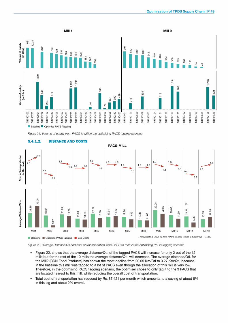
Optimisation of TPDS Supply Chain | P 49
5.4.1.2. DISTANCE AND COSTS
• Figure 22, shows that the average distance/Qtl. of the tagged PACS will increase for only 2 out of the 12 mills but for the rest of the 10 mills the average distance/Qtl. will decrease. The average distance/Qtl. for the Mill2 (BDN Food Products) has shown the most decline from 20.05 Km/Qtl to 3.27 Km/Qtl, because in the baseline this mill was tagged to a lot of PACS even though the allocation of this mill is very low. Therefore, in the optimising PACS tagging scenario, the optimiser chose to only tag it to the 3 PACS that are located nearest to this mill, while reducing the overall cost of transportation.
• Total cost of transportation has reduced by Rs. 87,421 per month which amounts to a saving of about 6% in this leg and about 2% overall.
Figure 21: Volume of paddy from PACS to Mill in the optimising PACS tagging scenario
Volu
me
of p
addy
(in
Qtls
.)Vo
lum
e of
pad
dy
(in Q
tls.)
Mill 1 Mill 91,
031
1,02
1
1,57
0
S109
0305
Baseline Optimise PACS Tagging
S109
0703
S109
0901
S109
0707
S109
0107
S109
0313
S109
0409
S109
0402
S109
0401
S109
0701
S109
0301
S109
0410
S109
0407
S109
0901
S109
0107
S109
0508
S109
0507
S109
0503
S109
0104
S109
0106
S109
0105
S109
0303
S109
0506
S109
0101
S109
0103
S109
0707
S109
0702
S109
0108
S109
0502
842
224
773
S109
0705
1,19
8
1,21
5
S109
0408
182
S109
0303
948
S109
0202
74
S109
0306
367
S109
0312
390
S109
0405
439
315
805
713
842
773
724
634
599
564
561
508
383
367
216
907
840
810
805
542
478
478
334
308
213
201
188
54 49
1,29
4
983
1,24
6
829
Figure 22: Average Distance/Qtl and cost of transportation from PACS to mills in the optimising PACS tagging scenario
67
Cos
t of t
rans
port
atio
n (in
Rs.
Lak
h)Av
erag
e D
ista
nce/
Qtls
Baseline Optimise PACS Tagging Please note a value of zero refers to cost which is below Rs. 10,000
36.0
8
23.8
5
20.0
8
3.27
21.9
3
19.0
8
14.6
3
13.1
6 22.9
2
15.8
0
17.9
1
18.8
7
17.8
6
13.4
2
12.0
8
11.6
6
29.0
8
22.8
9
20.8
5
14.5
9
18.3
6
8.26 13
.83
17.7
6
Mill1 Mill2 Mill3 Mill4 Mill5 Mill6 Mill7 Mill8 Mill9 Mill10 Mill11 Mill12
2.0
2.4
0.5
1.7
1.6 1.1 1.1
1.7
1.4
0.2
1.5
PACS-MILL
1.51.2 1.2 1.2
1.6 1.6
1.40.4
1.3
1.5
0.3
1.31.1
Leg Costs

P 50 | Optimise PACS tagging
5.4.2. GEOSPATIAL REPRESENTATION OF THE SUPPLY CHAIN NETWORK IN THE OPTIMISING PACS TAGGING SCENARIO
The geo representation of the baseline and the optimising PACS scenario shows reduction in the network complexity between PACS to Mill in this scenario. (Figure 23)
5.5. CHANGES REQUIRED TO IMPLEMENT THIS SCENARIOTECHNICAL CHANGE
• Changes to the P-PAS databases on tagging of nodes: i.e. tagging of PACS to mills in the P-PAS system
OPERATIONAL CHANGE
• Changes in the tagging in Leg 1 i.e. PACS to Mill.• Preparation of new allocation orders based on the changes in tagging in leg 1 from PACS to Mill. While
the changes do not impact the total quantity delivered to each mill, there are changes in the quantities received by mills from each PACS.
• Changes in the planning/execution, delivery schedules and pick up of paddy from PACS to mills.
Optimise PACS Tagging
Figure 23: Geo-Representation of tagging in the optimise PACS tagging scenario
Mill 1 Mill 2 Mill 3 Mill 4 Mill 5 Mill 6 Mill 7 Mill 8 Mill 9 Mill 10 Mill 11 Mill 12
Destination
BaselinePACS-MILL PACS-MILL

Optimisation of TPDS Supply Chain | P 51
CHAPTER6. 6
SCENARIO 3 OPTIMISE LEG 1 AND 2
CHAPTER

P 52 | Optimise leg 1 and 2
6.1. ABOUT THE SCENARIOIn this scenario, the model optimises leg 1 and 2 i.e. PACS to Mill and Mill to RRC, while keeping leg 3 i.e RRC to FPS as same. For Leg 1, both the tagging and allocation from PACS to Mill are optimised, while for Leg 2 only tagging from Mill to RRC is optimised, total volume allocated to each RRC has been kept the same. Additionally, while optimising, the volume that is allocated to each mill has been changes, while ensuring that it does not exceed the maximum capacity of that mill.
This scenario allows the optimisation model to choose from more possible routes and therefore it is possible to decrease the transportation costs by a lot more than in the optimising PACS scenario. Overall, the total cost saving is 11% or Rs. 5,07,710 per month. The costs for leg 1 have been reduced by 16% from the baseline and the cost for leg 2 have been reduced by 29% from the baseline.
SCENARIO: BASELINE
SCENARIO: OPTIMISE LEG 1 AND 2
TTC: Rs. 45,71,640 | ADT: 84 Km./Qtl. | ATC: 1.21 Rs. per Km./Qtl
TTC: Rs. 40,63,924 (-11%) | ADT: 70.7 Km./Qtl. | ATC: 1.38 Rs. per Km./Qtl.
**TTC - Total Transport Costs | ADT - Average Distance Travelled | ATC - Average Transportation Costs
6.2. KEY CONSTRAINTS1. All paddy that is procured is transported to one of the mills in the district.2. All paddy that is procured from the PACS is processed by the mills.3. All mills have an efficiency of 68%: for every Kg. of paddy that flows into the mill it produces exactly
0.68 Kg. of rice.4. All rice that is produced at the mills is transported to one of the 10 RRCs in Dhenkanal.5. FPS can only be supplied by a RRC that it’s connected to according to the current FPS tagging (this
holds for the supply of both rice and wheat). 6. All demand for rice and wheat at every FPS must be satisfied.7. The wheat allocation of every RRC is defined by the wheat demand of the connected FPSs. 8. All wheat demand in the district is fulfilled from FCI (Dhenkanal). 9. Rice delivered from RRC to FPS is as per the FPS allocation, any remaining quantity of rice is stored
for further use or transport to deficit districts.
Table 16: Summary statistics for scenario Optimising Leg 1&2
SCENARIO 3. OPTIMISE LEG 1 AND 2
Can be changed Remains the same Can be closed

Optimisation of TPDS Supply Chain | P 53
Baseline 15,69,794 1.09 19.5113,22,450 (-16%) 1.33 (+22%) 13.50 (-31%)Optimise Leg 1
and 2
Baseline 0.95 19.249,09,6311.09 (+15%) 11.87 (-38%)6,49,258 (-29%)Optimise Leg 1
and 2
Baseline 1.63 22.4016,44,524 1.63 22.4016,44,524Optimise Leg 1
and 2
Baseline 1.63 22.222,89,7501.63 22.222,89,750Optimise Leg 1
and 2Table 17: Key output KPI’s for optimising leg 1&2 scenario
Figure 24: Changes in total cost and distance in all legs for the scenario optimise leg 1 and 2
Baseline 1,57,941 0.86 22.92
1,57,941 0.86 22.92Optimise Leg 1 and 2
Wheat (8000 Qtls.)
Wheat (8000 Qtls.)
Rice (45,000 Qtls)
Rice (45,000 Qtls)
Paddy (73,529 Qtls)
Baseline Optimise Leg 1 and 2
PACS-MILL PACS-MILLMILL-RRC MILL-RRCFCI-RRC FCI-RRCRRC-FPS RRC-FPSRRC-FPS RRC-FPS
15.7
9.1
1.58
16.45
2.9
22.2222.4022.9219.2419.51
Aver
age
Dis
tanc
e/Q
tl.
Aver
age
Dis
tanc
e/Q
tl.
Cos
t of t
rans
port
atio
n (in
Rs.
Lak
h)
Cos
t of t
rans
port
atio
n (in
Rs.
Lak
h)
13.226.49
1.58
16.45
2.9
13.50 11.87
22.92 22.40 22.22
WHEATRICEPADDY
Total Transportation Costs (Rs. /month):
Average Transportation Costs (Rs. /Qtl. /Km.):
Average Distance Travelled (Km. /Qtl.):
6.3. KEY PERFORMANCE INDICATORS

P 54 | Optimise leg 1 and 2
6.4. CHANGES FROM THE BASELINEThe changes are restricted to Leg 1 and 2 of the supply chain. Overall the costs have reduced by 11% or Rs 5,07,710 per month. For Leg 1 average distance per Qtl. has reduced from 19.51 Km./Qtl to 13.50 Km./Qtl. and for Leg 2 from 19.24 Km./Qtl. to 11.87 Km./Qtl. Table 17 shows that the average transportation costs have increased in Leg 1 and 2. This is largely because the average transportation costs are dependent on total transportation costs, volume and distance (i.e. average transportation costs=total cost of transportation/ (volume*distance) and while distance has reduced by 56% and 82% respectively for leg 1 and 2 due to optimisation the cost of transportation in these legs has only reduced by 16% and 29%.
OBSERVATIONS FOR LEG 1: PACS TO MILL
6.4.2.1. TAGGING AND VOLUME
• Tagging and volume from PACS to Mill have been reallocated to optimise the overall costs. For example: Mill 1(Annapurna rice mill) was tagged to 13 PACS in the baseline, but after the optimisation, allocation to the mill has been reduced from 8,222 Qtls. to 2040 Qtls and the number of PACS tagged to it have reduced to 2. On the other hand, tagging to Mill 2 (BDN Food Products) has reduced, but allocation has been increased six times than the baseline.
• Number of nodes traversed in this leg have decreased from 125 to 84. (Figure 25).
6.4.2.2. DISTANCE AND COSTS
13 1412
10
15
108
1614
11
Figure 25: Tagging and volume of paddy from PACS to mills in the optimising leg 1&2 scenario
Volu
me
of p
addy
(Q
tls.)
8,222
2,040 2,630
Cou
nt o
f PAC
S Ta
gged
to M
ills
(Qtls
.)
PACS-MILL12,415
7,335
1,345
5,983
3,724
6,975
8,3147,314
2,974
6,058
7,657
7,212
14,118
6,184
805
6,7548,794
7,097
9,181
2,163 1,764
Mill12Mill11Mill10Mill9Mill8Mill7Mill6Mill5Mill4Mill3Mill2Mill1
Baseline Optimise Leg 1 and 2
2 25
12
11 57
10
1 24
117
Figure 26: Distance and cost of transportation from PACS to mills in the optimising leg 1 and 2 scenario
67
PACS-MILL
Cos
t of t
rans
port
atio
n (in
Rs.
Lak
h)Av
erag
e D
ista
nce/
Qtl
23.85
36.08
2.0
0.5
1.7
1.1 1.1
1.7 1.5 1.51.2 1.2 1.2
1.6 1.6
1.4
0.41.3
1.5
0.3
1.31.1
1.41.6
0.2
2.4
20.05
3.27
21.93 19.0814.63 13.16
22.9215.80 17.91 18.87 17.86
13.42 12.08 11.66
29.0822.89 20.85
14.5918.36
8.2613.83
17.76
Mill12Mill11Mill10Mill9Mill8Mill7Mill6Mill5Mill4Mill3Mill2Mill1
Baseline Optimise Leg 1 and 2 Leg Costs
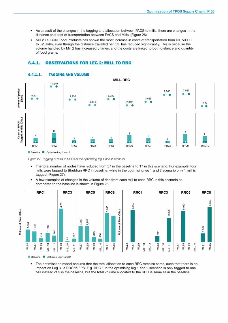
Optimisation of TPDS Supply Chain | P 55
• As a result of the changes in the tagging and allocation between PACS to mills, there are changes in the distance and cost of transportation between PACS and Mills. (Figure 26).
• Mill 2 i.e. BDN Food Products has shown the most increase in costs of transportation from Rs. 50000 to ~2 lakhs, even though the distance travelled per Qtl. has reduced significantly. This is because the volume handled by Mill 2 has increased 5 times, and the costs are linked to both distance and quantity of food grains.
6.4.1. OBSERVATIONS FOR LEG 2: MILL TO RRC
6.4.1.1. TAGGING AND VOLUME
Figure 27: Tagging of mills to RRCs in the optimising leg 1 and 2 scenario
• The total number of nodes have reduced from 57 in the baseline to 17 in this scenario. For example, four mills were tagged to Bhubhan RRC in baseline, while in the optimising leg 1 and 2 scenario only 1 mill is tagged. (Figure 27).
• A few examples of changes in the volume of rice from each mill to each RRC in this scenario as compared to the baseline is shown in Figure 28.
• The optimisation model ensures that the total allocation to each RRC remains same, such that there is no impact on Leg 3 i.e RRC to FPS. E.g. RRC 1 in the optimising leg 1 and 2 scenario is only tagged to one Mill instead of 5 in the baseline, but the total volume allocated to the RRC is same as in the baseline.
12
Volu
me
of p
addy
(Q
tls.)
MILL-RRC
Cou
nt o
f PAC
S Ta
gged
to M
ills
(Qtls
.)
Baseline
RRC1
5
5,207
11,040
4,750
2,144
5,020
2,0223,639
7,040 7,547
1,592
10
3 4 48
52
97
1 5 2RRC2 RRC3 RRC4 RRC5 RRC6 RRC7 RRC8 RRC9 RRC10
Optimise Leg 1 and 2
1 1 1 1 1 2
RRC1
Baseline Optimise Leg 1 and 2
Volu
me
of R
ice
(Qtls
.)
RRC1RRC3 RRC3RRC5 RRC5RRC8 RRC8
MIL
L41,
554
1,32
1
438
1,11
3
780
4,28
1
82
MIL
L7
MIL
L9
MIL
L10
MIL
L12
MIL
L3
MIL
L10
MIL
L11
MIL
L11
MIL
L7
MIL
L8
MIL
L8
MIL
L9
MIL
L9
MIL
L10
MIL
L1
MIL
L1
MIL
L5
MIL
L5
MIL
L4
MIL
L7
MIL
L7
MIL
L3
MIL
L9
MIL
L10
MIL
L10
MIL
L10
MIL
L12
387
2,00
2
1,98
7
3,69
6 5,20
7
914
645
386
3,83
6 5,02
0
1,38
7
5,65
3
Volu
me
of R
ice
(Qtls
.)

P 56 | Optimise leg 1 and 2
6.4.1.2. DISTANCE AND COSTS
Figure 29, describes the changes in the average distance/Qtl and the total cost for transportation in Leg 2 for the optimising leg 1 and 2 scenario. Cost of transportation has reduced for all nodes between Mill to RRC due to changes in tagging and distance travelled between nodes.
6.4.2. GEOSPATIAL REPRESENTATION OF THE SUPPLY CHAIN NETWORK IN OPTIMISING LEG 1 AND 2
The maps display the tagging of PACS to Mill and Mill to RRC. It can be observed that the transportation of paddy from east to west has been rationalised, thereby reducing the overall costs without change in the supply volume (demand) of the FPS and RRCs. (Figure 30, 31).
Figure 30: Geo-representation of tagging between PACS and mills in the optimising leg 1 and 2 scenario
Mill 1 Mill 2 Mill 3 Mill 4 Mill 5 Mill 6 Mill 7 Mill 8 Mill 9 Mill 10 Mill 11 Mill 12
Destination
Baseline Optimise Leg 1 & 2PACS-MILL PACS-MILL
Figure 29: Distance and costs of transportation from mills to RRCs in the optimising leg 1 and 2 scenario
Cos
t of t
rans
port
atio
n (in
Rs.
Lak
h)Av
erag
e D
ista
nce/
Qtl.
RRC1
26.64
2.61
28.55
14.23 13.38
25.35 27.29
3.77 5.39 5.97
18.51
0.2
0.31.0
1.4
0.1
0.3
0.1
0.5
1.1
0.2
2.7 2.7
0.3
0.0
1.1
0.90.6 0.6
9.51
17.64
8.682.70
16.1428.65
8.72
1.48
RRC2 RRC3 RRC4 RRC5 RRC6 RRC7 RRC8 RRC9 RRC10
Baseline Optimise Leg 1 and 2 Leg Costs Please note that a value of zero refers to costs which are below Rs.10,000
5.70
MILL-RRC
0.6
0.8

Optimisation of TPDS Supply Chain | P 57
Figure 31: Geo-representation of tagging between Mill and RRC in the optimising leg 1 and 2 scenario
6.5. CHANGES REQUIRED TO IMPLEMENT THE SCENARIOTECHNICAL CHANGE
• Changes to the SCMS and P-PAS databases on tagging of nodes: i.e. tagging of mills to RRCs in SCMS and tagging of PACS to mills in the P-PAS system.
• Changes to the P-PAS and miller database on the allocation of grains to mills i.e. allocation of mills in P-PAS.
OPERATIONAL CHANGE
• Changes to existing contracts/prepare new contract for the next procurement cycle for mills to accommodate transportation and other changes as a result of revised tagging and allocation.
• Changes in the tagging and volume from PACS to Mills and changes in tagging for Mills to RRC. • Preparation of new allocation orders based on the changes in tagging of PACS to Mills and Mills to RRC.
While the changes do not impact the total quantity delivered to each RRC, there are changes in the quantities received by RRC from each Mill.
• Changes in the planning/execution, delivery schedules and pick up of paddy from PACS to Mills and Mills to RRC.
RRC 1 RRC 2 RRC 3 RRC 4 RRC 5 RRC 6 RRC 7 RRC 8 RRC 9 RRC 10
Destination
Baseline Optimise Leg 1 & 2MILL-RRC MILL-RRC

P 58 | Optimise leg 1 and 2

Optimisation of TPDS Supply Chain | P 59
CHAPTER7. 7
SCENARIO 4OPTIMISE FPS TAGGING
CHAPTER

P 60 | Optimise FPS tagging
7.1. ABOUT THE SCENARIOIn this scenario, changes are made only in the tagging of FPS to RRC, while the configuration (tagging and volume) of leg 1 and 2, i.e PACS to mills and mills to RRC remains the same as in the baseline. Under the current transport contract for the last leg i.e. RRC to FPS, it is not possible to minimise the costs because the costs are only dependent on volume (i.e per Qtl defined per block) and not on travelled distance (Refer table 4 in section 2.3 for the details on costs). Additionally, in this scenario the volume allotted to each FPS is not altered to ensure fulfillment of demand at FPS, therefore costs savings cannot be achieved unless the changes in tagging and resultant decrease in distance is reflected in the transport cost. Thus, to analyse these savings for this scenario, the calculated costs of transportation for leg 3 i.e. RRC to FPS (refer to Table 9) of Rs.1.63 per Qtl. per Km. have been used.
Overall, with the changes in tagging and change in contract modality from exsiting per Qtl. cost to the calculated rate which is per Qtl. per Km. overlooking the administrative boundaries of the block, 9% cost savings from the baseline can be achieved.
SCENARIO: BASELINE
SCENARIO: OPTIMISE FPS TAGGING
TTC: Rs. 45,71,640 | ADT: 84 Km./Qtl. | ATC: 1.21 Rs. per Km./Qtl
TTC: Rs. 41,80,933 (-9%) | ADT: 79.5 KM./QTL. | ATC: 1.19 RS. PER KM./QTL.
**TTC - Total Transport Costs | ADT - Average Distance Travelled | ATC - Average Transportation Costs
7.2. KEY CONSTRAINTS1. Every PACS can only supply a mill that it’s connected to according to the current PACS tagging.2. All paddy that is procured is transported to one of the mills in the district.3. All paddy that is procured from the PACS is processed by the mills.4. All mills have an efficiency of 68%: for every Kg. of paddy that flows into the mill it produces exactly
0.68 Kg. of rice.5. The volumes of rice that are being transported from mills to RRCs are given by the data.6. All rice that is produced at the mills is transported to one of the 10 RRCs in Dhenkanal.7. All demand for rice and wheat at every FPS must be satisfied.8. All wheat demand in the district is fulfilled from FCI (Dhenkanal). 9. Rice delivered from RRC to FPS is as per the FPS allocation, any remaining quantity of rice is stored
for further use or transport to deficit districts.
Table 18: Summary statistics for scenario optimising FPS tagging
SCENARIO 4. OPTIMISE FPS TAGGING
Can be changed Remains the same Can be closed

Optimisation of TPDS Supply Chain | P 61
Figure 32: Total distance and cost of transportation for all legs in the optimising FPS tagging scenario
Baseline Optimise FPS Tagging
WHEATRICEPADDY
Aver
age
Dis
tanc
e/Q
tl.
Aver
age
Dis
tanc
e/Q
tl.
Cos
t of t
rans
port
atio
n (in
Rs.
Lak
h)
Cos
t of t
rans
port
atio
n (in
Rs.
Lak
h)
PACS-MILL PACS-MILLMILL-RRC MILL-RRCFCI-RRC FCI-RRCRRC-FPS RRC-FPSRRC-FPS RRC-FPS
15.7
9.11.58
16.45
2.90
19.51 19.24 22.92 22.40 22.22 19.51 19.24 22.92 18.08 16.65
15.7
9.11.58
13.26
2.17
Table 19: Key output KPI’s for optimising leg 1&2 scenario
Baseline 15,69,794 1.09 19.5115,69,794 1.09 19.51Optimise FPS
Tagging
Baseline 0.95 19.249,09,6310.95 19.249,09,631Optimise FPS
Tagging
Baseline 1.63 22.4016,44,524 1.63 18.08 (-19%)13,26,471 (-19%)Optimise FPS
Tagging
Baseline 1.63 22.222,89,7501.63 16.65 (-25%)2,17,095 (-25%)Optimise FPS
Tagging
Baseline 1,57,941 0.86 22.92
1,57,941 0.86 22.92Optimise FPS Tagging
Wheat (8000 Qtls.)
Rice (45,000 Qtls)
Rice (45,000 Qtls)
Paddy (73,529 Qtls)
Wheat (8000 Qtls.)
7.3. KEY PERFORMANCE INDICATORSTotal Transportation Costs (Rs. /month):
Average Transportation Costs (Rs. /Qtl. /Km.):
Average Distance Travelled (Km. /Qtl.):

P 62 | Optimise FPS tagging
7.4. CHANGES FROM THE BASELINEChanges are made only to the last leg i.e. RRC to FPS, hence all the observation relate to only this leg. Overall the cost savings are 9% from the baseline or Rs. 3,90,707 monthly. Below are the key changes:
7.4.1. OBSERVATIONS FOR LEG 3: RRC TO FPS
7.4.1.1. TAGGING AND VOLUME
There are changes to tagging of 356 out of 565 FPSs. Figure 33 describes the changes in tagging between baseline and the optimisation scenario for both rice and wheat.
Figure 33: Tagging of FPS to RRCs (Rice) in the optimising FPS tagging scenario
Cou
nt o
f FPS
Tag
ged
to R
RC
Volu
me
(Qtls
.)
5,674
11,761
4,777
2,329
5,703
2,9063,639
7,442 7,381
1,783
74
142
5140
48
86
43
111 105
38
Mill10Mill9Mill8Mill7Mill6Mill5Mill4Mill3Mill2Mill1
Baseline Optimise FPS Tagging
74
38
110 104
30
74
43 36
122
RRC-FPS
Figure 34: Volume of rice and wheat from RRC to FPS in each block in the optimise FPS tagging scenario
Volu
me
(Qtls
.)
RRC
2
Baseline Optimise FPS Tagging
3,79
1
17
RRC
5
RRC
6
RRC
7
RRC
9
RRC
10
RRC
2
RRC
6
RRC
8
RRC
9
RRC
10
RRC
4
RRC
6
RRC
7
RRC
9
RRC
2
RRC
6
RRC
8
RRC
9
RRC
2
RRC
3
RRC
4
RRC
6
RRC
7
RRC
9
RRC
10
RRC
10
Num
ber
of F
PS
BHUBAN HINDOL KAMAKHYANAGAR ODAPADA PARAJANG
125
374
19 58 631
604
51 395
3,05
2
444
88
1,58
6
3,19
3
3,94
2
5206,
237
1,46
0
254
463
136
1Num
ber
of F
PS
1 4
58
1 7 17 16
57
6
3349
70
10
2
1
69
17
42
8 10 2
5757
1222 11118
63
208
172
55
Volu
me
(Qtls
.)
4,22
0
353
138
16
3,61
3
131
170
84
7,35
8
6,50
7
510
3,10
4
2,32
9
180

Optimisation of TPDS Supply Chain | P 63
For some blocks the tagging has changed drastically e.g. Odapada and Bhubhan, where during the analyis it can be observed that most of the Fair Price Shops are tagged to a different RRC in the baseline. It can also be observed that for some blocks the tagging remains largely the same e.g. Parjang, Hindol. (Figure 34)
7.4.1.2. DISTANCE AND COSTS
• Maximum FPS are tagged within a distance of 0-50 km from the tagged RRC, with an upward shift from 89 in the baseline to 139 within the 0-10 km distance in the revised FPS tagging. Number of FPS in the 50-90 Km ranges has been reduced from the tagged RRC 65 to 23. Overall, the average distance from RRC to FPS hs been reduced by 21%.
• Figure 36, describes the cost of transport from each RRC to FPS for both rice and wheat. It can be observed that costs have come down for each RRC except for RRC 2 (Baladiabandha).
• As per the current/prevalent transportation contract the cost of transportation is dependant only on the volume (Rs./Qtl.), this combined with the restriction of block boundries results in higher costs to GoO. Thus to calculate the cost savings due to change in tagging and distance between nodes, the derived rate of Rs. 1.63 per Km. per Qtl. (refer table 9) has been used. At the derived cost, cost decrease of ~20% in the last leg which results in an overall saving of 9% of total costs can be achieved.
Figure 35: Distance travelled by FPS in the leg: RRC to FPS in the optimising FPS tagging scenario
Num
ber o
f FPS
13
139
0-10Km.
Baseline Optimise FPS Tagging
10-20Km. 20-30Km. 30-40Km. 40-50Km.
Distance RRC- FPS
50-60Km. 60-70Km. 70-80Km. 80-90Km.
157132
89
48 4120
31236
88
129145
87
Figure 36: Cost of transportation from RRC to FPS in the scenario optimising FPS tagging
RRC-FPS
20.0
5
3.27
Baseline
21.30
1.9
1.6
4.8
1.5
1.00.7
2.5
1.41.2 1.1
2.4 2.6
1.62.3
0.6 0.6
0.8 0.80.6
RRC1 RRC2 RRC3 RRC4 RRC5 RRC6 RRC7 RRC8 RRC9 RRC10
41.09
25.82
16.8412.94 12.46
15.46
25.33
15.71 18.11 16.1913.66 13.05 13.00 12.83 15.22
18.7414.62
19.8517.34
Aver
age
Dis
tanc
e (Q
tls.)
Cos
t of t
rans
port
atio
n (in
Rs.
Lak
h)
Optimise FPS Tagging Leg Costs
5.0

P 64 | Optimise FPS tagging
Figure 37, shows the savings at the derived rate of Rs. 1.63 per Km. per Qtl. as well as the range over which savings are feasible in this optimisation scenario. The graph shows that if the transportation rate is below Rs. 1.63 per Km. per Qtl. then there are always savings. However, if the costs are between Rs. 1.63 and Rs. 2.04 per Km. per Qtl. then savings are feasible only if tagging of RRC to FPS is optimised. At a rate which is above Rs. 2.04 per Km. per Qtl. costs will be higher than exsiting prevelant costs, hence GoO should aim to keep the rate less than Rs. 2.04 per Km. per Qtl.
7.4.2. GEOSPATIAL REPRESENTATION OF THE SUPPLY CHAIN NETWORK IN OPTIMISING FPS TAGGING
Figure 38, represents the tagging of RRCs to FPS. FPS tagging is now more clustered, which could be used for contracting transporter. The inefficiencies where grain was travelling from west to east have also been rationalised.
Figure 38: Geo-representation of tagging from RRC to FPS in the optimising FPS tagging scenario
RRC 1 RRC 2 RRC 3 RRC 4 RRC 5 RRC 6 RRC 7 RRC 8 RRC 9 RRC 10
Origin
BaselineRRC-FPS
Optimise FPS TaggingRRC-FPS
Figure 37: Analysis of savings over a range of transportation rates for the last leg
Cur
rent
Cos
t of T
rans
port
atio
n (R
s.)
Average Cost per Qtl. per Km
` 500,000
` 700,000
` 900,000
` 1,100,000
` 1,300,000
` 1,500,000
` 1,700,000
` 1,900,000Current cost of transportation
20%
1.30 1.35 1.40 1.45 1.50 1.55 1.60 1.65 1.70 1.75 1.80 1.85 1.90 1.95 2.00 2.05 2.10 2.15 2.20 2.25 2.30
Baseline
Optimise FPS Tagging
` 2,100,000
` 2,300,000
` 2,500,000
` 2,700,000
` 2,900,000
Only save if you optimise FPS Tagging Never Save

Optimisation of TPDS Supply Chain | P 65
7.5. CHANGES REQUIRED TO IMPLEMENT THIS SCENARIO POLICY CHANGES
• Classification of supply zones in the food security rules and assigning of responsibilities.• Revision in the methodology for contracting of transporters including contracting terms, transportation
rate etc. to accommodate recommendation to move from per Qtl. rate to per Qtl. per Km. rate for the last leg i.e. RRC to FPS.
TECHNICAL CHANGE
• Changes to the SCMS and FPS automation systems on tagging of nodes: i.e. tagging of RRC to FPS for allocation, movement and receipt of grains.
OPERATIONAL CHANGE
• Contracting of new transport agents (L2 transporters) or changes to existing contracts to accommodate changes in rates of transportation, allocation and tagging.
• Preparation of new allocation orders based on the changes in tagging of RRC.• Changes in the planning/execution, delivery schedules and pick up of rice and wheat from RRC’s to FPS.

P 66 | Optimise FPS tagging

Optimisation of TPDS Supply Chain | P 67
CHAPTER8. 8
SCENARIO 5CLOSING MILLS
CHAPTER

P 68 | Closing Mills
8.1. ABOUT THE SCENARIOThis scenario quantifies the impact of closing a few mills in Dhenkanal district and its impact on the total transportation costs. This scenario is similar to Scenario 3: Optimising leg 1 & 2, with additional conditions which include: each mill is either be closed or used to its full capacity to maximise the usage of available resources, and that the volume at each RRC is kept same as in the baseline. The average transportation costs in this scenario will be higher because closing down some mills will increase the distance that each Qtl. of paddy and rice has to travel to and from the mills. Overall, the cost savings in this scenario are 6% from the baseline or Rs. 2,79,565, with savings of 10% and 14% in Leg 1 and 2 respectively.
SCENARIO: BASELINE
SCENARIO: CLOSING MILLS
TTC: Rs. 45,71,640 | ADT: 84 Km./Qtl. | ATC: 1.21 Rs. per Km./Qtl
TTC: RS. 42,92,075 (-6%) | ADT: 76.2 KM./QTL. | ATC: 1.31 RS. PER KM./QTL.
**TTC - Total Transport Costs | ADT - Average Distance Travelled | ATC - Average Transportation Costs
8.2. KEY CONSTRAINT1. All paddy that is procured must be transported to one of the mills in the district.2. All paddy that is procured from the PACS must be processed by the mills.3. All mills have an efficiency of 68%. For every Kg. of paddy that flows into the mill it produces exactly
0.68 Kg. of rice.4. All rice that is produced at the mills is transported to one of the 10 RRCs in Dhenkanal.5. All demand for rice and wheat at every FPS must be satisfied.6. All wheat demand flows into the district at the FCI (Dhenkanal).7. Each FPS can only be supplied by a RRC that it’s connected to according to the current FPS tagging
(this holds for the supply of both rice and wheat). 8. The wheat allocation of every RRC is defined by the wheat demand of the connected FPSs.9. Rice delivered from RRC to FPS is as per the FPS allocation, any remaining quantity of rice is stored
for further use or transport to deficit districts. 10. Each mill should either be closed or it should be used to 90% of its full capacity in order to maximise
the usage of available resources.
Table 20: Summary statistics for the scenario closing mills
SCENARIO 5. CLOSING MILLS
Can be changed Remains the same Can be closed
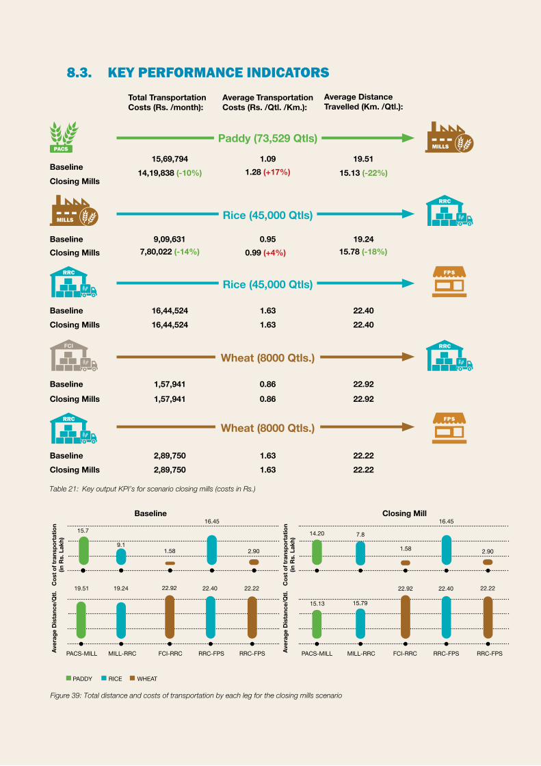
Optimisation of TPDS Supply Chain | P 69
15,69,794 1.09 19.5114,19,838 (-10%) 1.28 (+17%) 15.13 (-22%)
0.95 19.249,09,6310.99 (+4%) 15.78 (-18%)7,80,022 (-14%)
1.63 22.4016,44,524 1.63 22.4016,44,524
1.63 22.222,89,7501.63 22.222,89,750
Table 21: Key output KPI’s for scenario closing mills (costs in Rs.)
Figure 39: Total distance and costs of transportation by each leg for the closing mills scenario
1,57,941 0.86 22.92
1,57,941 0.86 22.92
Baseline Closing Mill
WHEATRICEPADDY
PACS-MILL PACS-MILLMILL-RRC MILL-RRCFCI-RRC FCI-RRCRRC-FPS RRC-FPSRRC-FPS RRC-FPS
15.7
9.11.58
16.45 16.45
2.90 2.90
Aver
age
Dis
tanc
e/Q
tl.
Aver
age
Dis
tanc
e/Q
tl.
Cos
t of t
rans
port
atio
n (in
Rs.
Lak
h)
Cos
t of t
rans
port
atio
n (in
Rs.
Lak
h)
19.51 19.24 22.92 22.40 22.22
14.20 7.8
1.58
15.13 15.79
22.92 22.40 22.22
8.3. KEY PERFORMANCE INDICATORS
Baseline
Total Transportation Costs (Rs. /month):
Average Transportation Costs (Rs. /Qtl. /Km.):
Average Distance Travelled (Km. /Qtl.):
Closing Mills
BaselineClosing Mills
BaselineClosing Mills
BaselineClosing Mills
Baseline
Closing Mills
Wheat (8000 Qtls.)
Wheat (8000 Qtls.)
Rice (45,000 Qtls)
Rice (45,000 Qtls)
Paddy (73,529 Qtls)

P 70 | Closing Mills
8.4. CHANGES FROM THE BASELINEThe optimiser chooses to close 6 out of 12 mills and only keeps the ones that are relatively centrally located within the district. While, closure of mills impacts all legs of the supply chain in this scenario, a constraint has been placed that the volume at each RRC be kept same. Thus, the observations in the sections below are for Leg1 and 2 only. Overall the average cost of transportation for both leg 1 and 2 has increased, but the total costs have reduced by Rs. 1.5 lakhs and Rs. 1.3 lakh monthly for Leg 1 and 2 respectively.
8.4.1. OBSERVATIONS FOR LEG 1: PACS TO MILL
8.4.1.1. TAGGING AND VOLUME
• Figure 40, shows the change in allocation to mill across the baseline and closing mills scenarios. Overall Mill 8 i.e. Maa Tareni Rice mill has been allocated the highest volume of paddy.
• The number of nodes traversed from PACS to mills have reduced from 125 to 85 in this scenario.• It can be observed that if in the optimise leg 1 & 2 scenario allocation to a mill was reduced in comparison
to the baseline, in the closing mills scenario the mill has been closed. (Refer figure 26, 40)• In cases where in the optimise leg 1 & 2 scenario, the throughput of the mill has been increased in
comparison to the baseline, in this scenario mill is assigned to it full capacity. These results are on expected lines, since in both scenarios utilisation is determined by the proximity to the PACS and RRCs.
8.4.1.2. DISTANCE AND COSTS
Baseline Closing Mills
Figure 40: Changes in tagging and volume from PACS to mills in the closing mills scenario
Cou
nt o
f PAC
S Ta
gged
to
Mill
sVo
lum
e of
pad
dy (Q
tls.)
PACS-MILL
11,250
7,335 5,983
6,975 7,314
9,000
6,058 7,212
18,000
6,184 6,754
1,764
14,400
7,097
13,500
7,379
2,630
8,222
13
Mill1 Mill2 Mill3 Mill4 Mill5 Mill6 Mill7 Mill8
1412 10
12 12 11
21
1411
18
711 108 10
4
Mill10 Mill11 Mill12Mill9
Figure 41: Distance and cost of transportation from PACS to Mills in the closing mills scenario
67
Aver
age
Dis
tanc
e (Q
tl.)
Cos
t of t
rans
port
atio
n (in
Rs.
Lak
h)
PACS-Mill
2.0
Mill1
23.8520.05 21.93
14.6312.23
Baseline Closing Mills Legs Costs
Mill2 Mill3 Mill4 Mill5 Mill6 Mill7 Mill8 Mill9 Mill10 Mill11 Mill12
0.5
1.9 1.71.1
1.7
1.4 1.51.2 1.2
3.5 3.3
1.6 1.6
0.4
1.3
2.41.7
22.92
13.9817.91
14.83 17.8612.27 12.08 14.08
29.08
20.8518.36
21.2713.83

Optimisation of TPDS Supply Chain | P 71
• Figure 41, describes the changes in distance and cost of transportation with closing of 6 out of 12 mills. Overall, the distance has reduced by 1,310 Km. and costs have reduced by Rs. 1.5 lakhs per month.
• It can be observed that cost has increased for most mills, but even then, the total cost in this leg has reduced by 10%. Highest cost increase has been for Mills 8 and Mill 11, since both tagging and volume allocated to these mills have increased.
8.4.2. OBSERVATIONS FOR LEG 2: MILL TO RRC
8.4.2.1. TAGGING AND VOLUME
• Figure 42, describes the revised tagging between mills and RRC after closing 6 mills. The number of nodes traversed have decreased from 57 to 15.
• Out of 10 RRC’s, 5 are tagged to only 1 Mill, while in the baseline they were tagged to as high as 9,10 mills. The changes to tagging have been done while ensuring that the total volume at each RRC remains same.
Figure 43: Changes in volume of rice from mills to RRC in the closing mills scenario
Volu
me
of R
ice
(Qtls
.)Vo
lum
e of
Ric
e (Q
tls.)
RRC1 RRC5 RRC7 RRC10
1,55
4M
ILL4
1,32
15,
207
MIL
L7
MIL
L10
1,11
3
MIL
L73,
233
2,00
2
MIL
L81,
787
1,98
7
MIL
L964
5
MIL
L10
386
MIL
L774
121
7
1M
ILL9
861
MIL
L10
329
MIL
L11
2,89
852
MIL
L210
314
6
MIL
L914
6
MIL
L10
124
MIL
L12
230
MIL
L424
8
MIL
L824
8
MIL
L61,
488
450
6M
ILL1
22,
180
MIL
L12
780
MIL
L943
8
Baseline Closing Mills
Figure 42: Tagging of mills to RRC in the closing mills scenario
Cou
nt o
f Mill
s Ta
gged
to
eac
h R
RC
Volu
me
(Qtls
.)
Baseline Closing Mills
11,040
10
2RRC2
5,207
5
1RRC1
4,750
3
1RRC3
10
7,040
2
RRC8
2,144
4
RRC41
2,022
8
RRC61
7,547
9
RRC91
12
5,020
4
RRC52
8
3,639
5
RRC72
1,592
7
RRC102
MILL-RRC
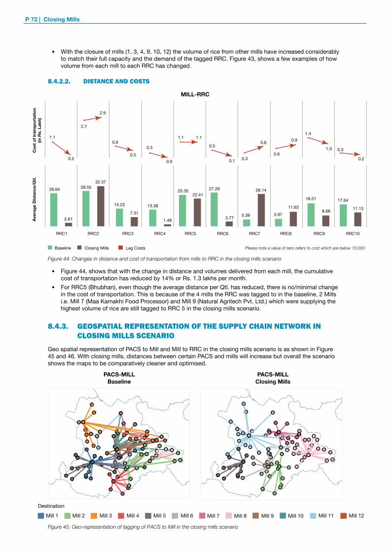
P 72 | Closing Mills
• With the closure of mills (1, 3, 4, 9, 10, 12) the volume of rice from other mills have increased considerably to match their full capacity and the demand of the tagged RRC. Figure 43, shows a few examples of how volume from each mill to each RRC has changed.
8.4.2.2. DISTANCE AND COSTS
• Figure 44, shows that with the change in distance and volumes delivered from each mill, the cumulative cost of transportation has reduced by 14% or Rs. 1.3 lakhs per month.
• For RRC5 (Bhubhan), even though the average distance per Qtl. has reduced, there is no/minimal change in the cost of transportation. This is because of the 4 mills the RRC was tagged to in the baseline, 2 Mills i.e. Mill 7 (Maa Kamakhi Food Processor) and Mill 9 (Natural Agritech Pvt. Ltd.) which were supplying the highest volume of rice are still tagged to RRC 5 in the closing mills scenario.
8.4.3. GEOSPATIAL REPRESENTATION OF THE SUPPLY CHAIN NETWORK IN CLOSING MILLS SCENARIO
Geo spatial representation of PACS to Mill and Mill to RRC in the closing mills scenario is as shown in Figure 45 and 46. With closing mills, distances between certain PACS and mills will increase but overall the scenario shows the maps to be comparatively cleaner and optimised.
Figure 45: Geo-representation of tagging of PACS to Mill in the closing mills scenario
BaselinePACS-MILL
Closing MillsPACS-MILL
Figure 44: Changes in distance and cost of transportation from mills to RRC in the closing mills scenario
12.2
3
12.2
7
Aver
age
Dis
tanc
e/Q
tl.
26.64
14.23
7.3113.38
1.48
25.3522.41
27.29
3.77 5.39 5.9711.63
18.51
8.68
17.64
11.13
0.2
0.31.0
1.4
0.60.30.1
0.5
1.1
MILL-RRC
1.1
0.0
0.30.5
0.2
1.10.8 0.9
26.14
Cos
t of t
rans
port
atio
n (in
Rs.
Lak
h)
2.61
RRC10RRC9RRC8RRC7RRC6RRC5RRC4RRC3
28.5532.37
2.9
2.7
RRC2RRC1
Baseline Closing Mills Leg Costs Please note a value of zero refers to cost which are below 10,000
0.8
Mill 1 Mill 2 Mill 3 Mill 4 Mill 5 Mill 6 Mill 7 Mill 8 Mill 9 Mill 10 Mill 11 Mill 12
Destination
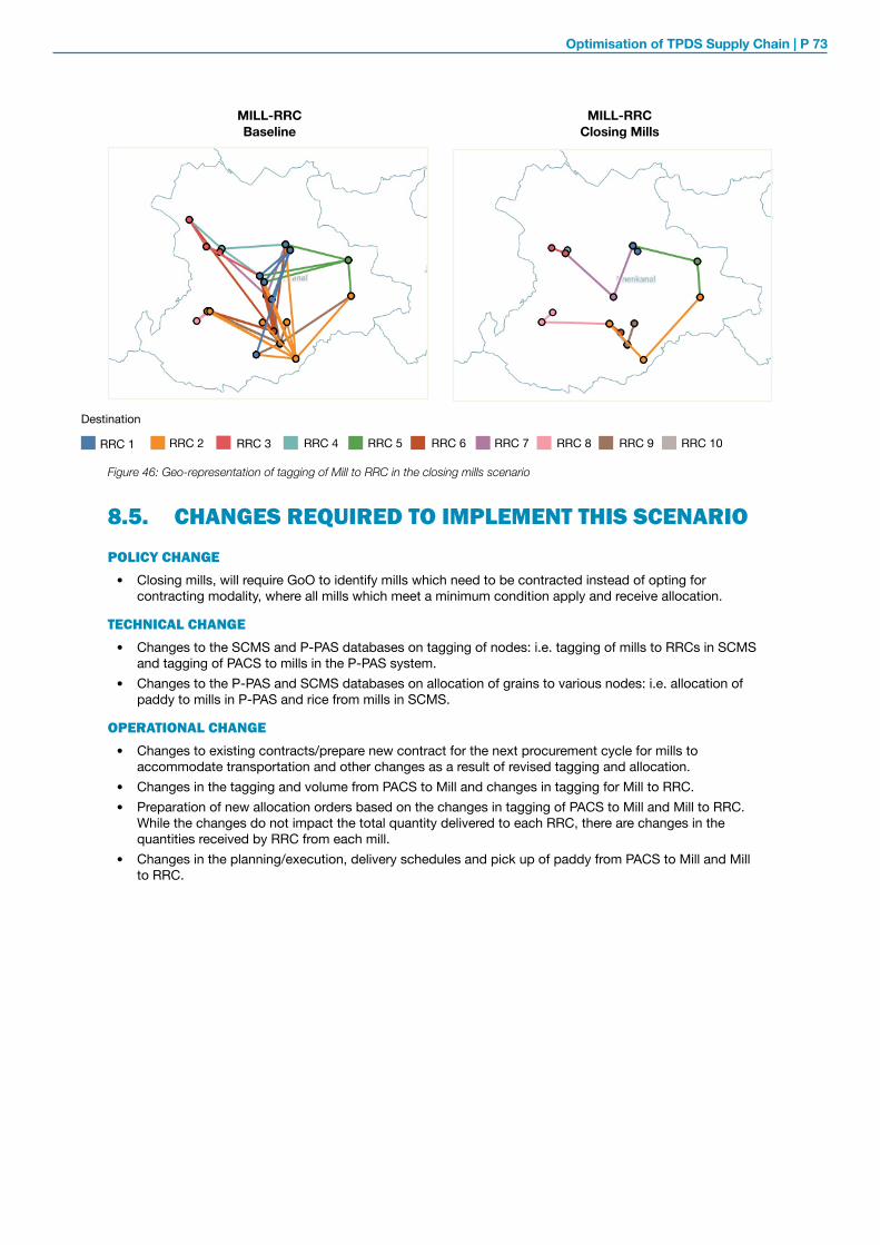
Optimisation of TPDS Supply Chain | P 73
8.5. CHANGES REQUIRED TO IMPLEMENT THIS SCENARIOPOLICY CHANGE
• Closing mills, will require GoO to identify mills which need to be contracted instead of opting for contracting modality, where all mills which meet a minimum condition apply and receive allocation.
TECHNICAL CHANGE
• Changes to the SCMS and P-PAS databases on tagging of nodes: i.e. tagging of mills to RRCs in SCMS and tagging of PACS to mills in the P-PAS system.
• Changes to the P-PAS and SCMS databases on allocation of grains to various nodes: i.e. allocation of paddy to mills in P-PAS and rice from mills in SCMS.
OPERATIONAL CHANGE
• Changes to existing contracts/prepare new contract for the next procurement cycle for mills to accommodate transportation and other changes as a result of revised tagging and allocation.
• Changes in the tagging and volume from PACS to Mill and changes in tagging for Mill to RRC. • Preparation of new allocation orders based on the changes in tagging of PACS to Mill and Mill to RRC.
While the changes do not impact the total quantity delivered to each RRC, there are changes in the quantities received by RRC from each mill.
• Changes in the planning/execution, delivery schedules and pick up of paddy from PACS to Mill and Mill to RRC.
Figure 46: Geo-representation of tagging of Mill to RRC in the closing mills scenario
BaselineMILL-RRC
Closing MillsMILL-RRC
RRC 1 RRC 2 RRC 3 RRC 4 RRC 5 RRC 6 RRC 7 RRC 8 RRC 9 RRC 10
Destination

P 74 | Closing Mills

Optimisation of TPDS Supply Chain | P 75
CHAPTER9.
SCENARIO 6CLOSING PACS
9CHAPTER
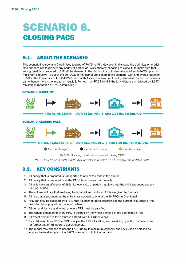
P 76 | Closing PACS
9.1. ABOUT THE SCENARIOThis scenario like scenario 2 optimises tagging of PACS to Mill. However, in this case the optimisation model also chooses not to procure any paddy at particular PACS, thereby choosing to close it. To make sure that enough paddy is procured to fulfil all the demand in the district, the optimiser allocated each PACS up to its maximum capacity. 12 out of the 80 PACS in the district are closed in this scenario, with and overall reduction of 5% in the total costs or Rs. 2,48,229 per month. Since, the volume of paddy allocated to each mill remains same, hence there is no impact on leg 2, 3. For leg 1 i.e. PACS to Mill, the total distance is reduced by 1,647 km resulting in reduction of 16% costs in leg 1.
SCENARIO: BASELINE
SCENARIO: CLOSING PACS
TTC: Rs. 45,71,640 | ADT: 84 Km./Qtl. | ATC: 1.21 Rs. per Km./Qtl
TTC: Rs. 43,23,411 (-5%) | ADT: 78.1 KM./QTL. | ATC: 1.30 RS. PER KM./QTL.
**TTC - Total Transport Costs | ADT - Average Distance Travelled | ATC - Average Transportation Costs
9.2. KEY CONSTRIANTS1. All paddy that is procured is transported to one of the mills in the district.2. All paddy that is procured from the PACS is processed by the mills.3. All mills have an efficiency of 68%: for every Kg. of paddy that flows into the mill it produces exactly
0.68 Kg. of rice.4. The volumes of rice that are being transported from mills to RRCs are given by the data.5. All rice that is produced at the mills is transported to one of the 10 RRCs in Dhenkanal.6. FPS can only be supplied by a RRC that it’s connected to according to the current FPS tagging (this
holds for the supply of both rice and wheat). 7. All demand for rice and wheat at every FPS must be satisfied.8. The wheat allocation of every RRC is defined by the wheat demand of the connected FPSs. 9. All wheat demand in the district is fulfilled from FCI (Dhenkanal). 10. Rice delivered from RRC to FPS is as per the FPS allocation, any remaining quantity of rice is stored
for further use or transport to deficit districts. 11. The model may choose to use the PACS up to its maximum capacity and PACS can be closed as
long as the total supply of the PACS is enough to fulfil the demand.
Table 22: Summary statistics for the scenario closing PACS
SCENARIO 6. CLOSING PACS
Can be changed Remains the same Can be closed

Optimisation of TPDS Supply Chain | P 77
15,69,794 1.09 19.5113,21,565 (-16%) 1.32 (+21%) 13.57 (-30%)
0.95 19.249,09,6310.95 19.249,09,631
1.63 22.4016,44,524 1.63 22.4016,44,524
1.63 22.222,89,7501.63 22.222,89,750
1,57,941 0.86 22.92
1,57,941 0.86 22.92
Figure 47: Total distance and costs of transportation for all legs in this scenario closing PACS
WHEATRICEPADDY
Aver
age
Dis
tanc
e/Q
tl.
Aver
age
Dis
tanc
e/Q
tl.
PACS-MILL PACS-MILLMILL-RRC MILL-RRCFCI-RRC FCI-RRCRRC-FPS RRC-FPSRRC-FPS RRC-FPS
Baseline Closing PACS
Cos
t of t
rans
port
atio
n (in
Rs.
Lak
h)
Cos
t of t
rans
port
atio
n (in
Rs.
Lak
h)
15.7
9.11.58
16.45
2.90
15.7
9.11.58
13.26
2.17
19.51 19.2422.92 22.40 22.22
13.5719.24
22.92 22.40 22.22
9.3. KEY PERFORMANCE INDICATORS
Baseline
Total Transportation Costs (Rs. /month):
Average Transportation Costs (Rs. /Qtl. /Km.):
Average Distance Travelled (Km. /Qtl.):
Closing PACS
BaselineClosing PACS
BaselineClosing PACS
BaselineClosing PACS
Baseline
Closing PACS
Paddy (73,529 Qtls)
Rice (45,000 Qtls)
Rice (45,000 Qtls)
Wheat (8000 Qtls.)
Wheat (8000 Qtls.)
Table 23: Key output KPI’s for scenario closing PACS

P 78 | Closing PACS
9.4. CHANGES FROM THE BASELINEThe optimal configuration in this case chooses to close 12 of the 80 PACS reducing the costs of leg 1 by 16% which is more than double of the cost savings in optimising PACS tagging scenario. The changes are restricted to leg 1 of the supply chain as there are changes only in the tagging of PACS to Mill and not in the volume of paddy allocated to each Mill.
9.4.1. OBSERVATIONS FOR LEG 1: PACS TO M ILL
9.4.1.1. TAGGING AND VOLUME
• Tagging of PACS to Mill has been optimised under the given constraints. The number of nodes traversed in leg 1 have reduced from 125 to 76. (Figure 48).
• Tagging of PACS to Mill 2 (BDN Food Products) and Mill 9 (Natural Agritech Pvt. Ltd.) has shown significant decline from 14 to 3 and 5 PACS respectively.
Even though there are significant changes in tagging of PACS, the change in volume procured by block is smaller. Kankadahad, Parajang and Dhenkanal block have the least change in volume procured, while Gandia and Bhuban block have the most impact in the procured volume. (Figure 49)
Figure 48: Tagging and volume of paddy from PACS to mills in the closing PACS scenario
Volu
me
of p
addy
(Q
tls)
Cou
nt o
f PAC
S Ta
gged
to
Mill
s
Baseline Closing PACS
Mill1
9
13
8,222
Mill23
14
2,630
Mill3
8
12
7,335
Mill4
7
10
5,983
Mill5
9
12
6,975
PACS-MILL
Mill7
5
8
6,058
Mill8
6
10
7,212
Mill9
5
14
6,184
Mill10
7
11
6,754
Mill113
4
1,764
Mill6
8
10
7,314 7,097
Mill12
6
7
Figure 49: Changes in tagging and volume of paddy by block in the closing PACS scenario
Cou
nt o
f PAC
S by
blo
ck
18
21 27
13 15
9
12 10
11,712
Volu
me
of p
addy
(Qtls
.)
5
14
9
1411
68 9 6,522
13,629
9,9018,963
13,141
6,3478,745
6,281
12,895
13,131
13,131
11,292
5,950
6,410
5,563
PARA
JAN
G
ODA
PADA
KAN
KADA
HAD
KAM
AKH
AYA
NAG
AR
KAM
AKH
AYA
NAG
ARHIN
DOL
GAN
DIA
DHEN
KAN
AL
BHU
BHAN
Baseline Closing Mills
HIN
DOL
GAN
DIA
DHEN
KAN
AL
BHU
BHAN
PARA
JAN
G
ODA
PADA
KAN
KADA
HAD

Optimisation of TPDS Supply Chain | P 79
9.4.1.2. DISTANCE AND COSTS
The cost of transportation to all the mills has reduced in leg 1 i.e.PACS to Mill. For Mill 2 (BDN Food Products) and Mill 9 (Natural Agritech Pvt. Ltd.), the average distance/Qtl had reduced significantly hence, the cost of transportation has also decreased. For Mill 12 (Tareni Agro Foods) the cost of transportation has increased, even through the number of PACS tagged has decreased from 7 to 6, because the averge distance/Qtl has increased.
9.4.2. GEOSPATIAL REPRESENTATION OF THE SUPPLY CHAIN NETWORK IN THE CLOSING PACS SCENARIO
Figure 51, shows that the tagging for leg 1 i.e. PACS to Mill is much more optimised than in the baseline. This results in efficiency in administration due to reduction in dependencies of multiple PACS to multiple mills. As an example Mill 3 was tagged to 12 PACS in the baseline, some of which were in the extreme east. In the closing PACS scenario, Mill 3 is tagged 8 PACS all of which are closer to the Mill.
Figure 51: Geo-representation of tagging of PACS to mills in the closing PACS scenario
BaselinePACS-MILL
Closing PACSPACS-MILL
Mill 1 Mill 2 Mill 3 Mill 4 Mill 5 Mill 6 Mill 7 Mill 8 Mill 9 Mill 10 Mill 11 Mill 12
Destination
67
Figure 50: Distance and cost of transportation from PACS to mills for the closing PACS scenario
Aver
age
Dis
tanc
e/Q
tl.C
ost o
f tra
nspo
rtat
ion
(in R
s. L
akh)
Baseline Closing PACS Leg Costs
Mill1
14.8220.05
3.47
21.9318.97
14.63
22.92
15.2517.91
15.1017.86
8.8012.08
8.96
29.08
10.24
20.8514.35
18.3613.83
19.90
7.0813.24
23.85
2.0
1.60.5
1.7
1.61.1
1.7
1.4
1.5
1.3
1.2
PACS-MILL
1.21.6 1.6
1.40.4
0.2
1.3
1.5
0.91.10.9
0.2
Mill2 Mill3 Mill4 Mill5 Mill6 Mill7 Mill8 Mill9 Mill10 Mill11 Mill12

P 80 | Closing PACS
9.5. CHANGES REQUIRED TO IMPLEMENT THIS SCENARIOPOLICY CHANGES
• Changes in procurement policy for establishing a max distance range at which a PACS must be setup for registration and procurement from farmers.
TECHNICAL CHANGE
• Changes to the P-PAS, farmer and miller’s databases on tagging of nodes: i.e. tagging of PACS to Mill.• Changes to the P-PAS Databases on allocation of grains to each node: i.e. allocation to mills from each
PACS in P-PAS.
OPERATIONAL CHANGE
• To implement the scenario would require coordination with the Department of Co-operation, for the change in number and volume of paddy procured at PACS.
• Changes in the tagging of PACS to Mill.• Preparation of new procurement plan and allocation orders for PACS and mills for the current/new
procurement cycle.• Changes in the planning/execution, delivery schedules and pick up of paddy from PACS to mills.• An assessment to remap registered farmers to new PACS would be required, to ensure that the impact in
terms of cost and distance is minimised. • Notification of new procurement centres through various channels and awareness activities for farmers, to
ensure that they know which PACS they can now register and sell their paddy. 10
Optimisation of TPDS Supply Chain | P 81
10SCENARIO 7CLOSING FPS
CHAPTER
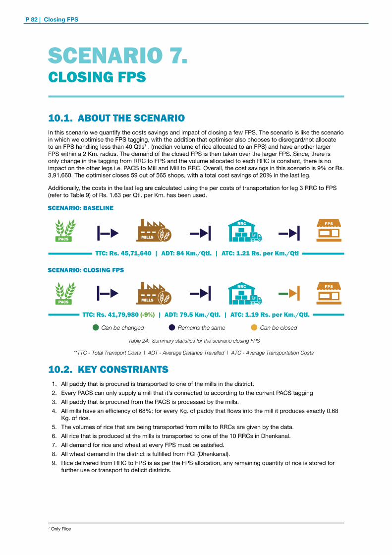
P 82 | Closing FPS
SCENARIO: BASELINE
SCENARIO: CLOSING FPS
TTC: Rs. 45,71,640 | ADT: 84 Km./Qtl. | ATC: 1.21 Rs. per Km./Qtl
TTC: Rs. 41,79,980 (-9%) | ADT: 79.5 Km./Qtl. | ATC: 1.19 Rs. per Km./Qtl.
**TTC - Total Transport Costs | ADT - Average Distance Travelled | ATC - Average Transportation Costs
10.2. KEY CONSTRIANTS1. All paddy that is procured is transported to one of the mills in the district.2. Every PACS can only supply a mill that it’s connected to according to the current PACS tagging 3. All paddy that is procured from the PACS is processed by the mills.4. All mills have an efficiency of 68%: for every Kg. of paddy that flows into the mill it produces exactly 0.68
Kg. of rice.5. The volumes of rice that are being transported from mills to RRCs are given by the data.6. All rice that is produced at the mills is transported to one of the 10 RRCs in Dhenkanal.7. All demand for rice and wheat at every FPS must be satisfied.8. All wheat demand in the district is fulfilled from FCI (Dhenkanal). 9. Rice delivered from RRC to FPS is as per the FPS allocation, any remaining quantity of rice is stored for
further use or transport to deficit districts.
Table 24: Summary statistics for the scenario closing FPS
SCENARIO 7. CLOSING FPS
10.1. ABOUT THE SCENARIOIn this scenario we quantify the costs savings and impact of closing a few FPS. The scenario is like the scenario in which we optimise the FPS tagging, with the addition that optimiser also chooses to disregard/not allocate to an FPS handling less than 40 Qtls7 . (median volume of rice allocated to an FPS) and have another larger FPS within a 2 Km. radius. The demand of the closed FPS is then taken over the larger FPS. Since, there is only change in the tagging from RRC to FPS and the volume allocated to each RRC is constant, there is no impact on the other legs i.e. PACS to Mill and Mill to RRC. Overall, the cost savings in this scenario is 9% or Rs. 3,91,660. The optimiser closes 59 out of 565 shops, with a total cost savings of 20% in the last leg.
Additionally, the costs in the last leg are calculated using the per costs of transportation for leg 3 RRC to FPS (refer to Table 9) of Rs. 1.63 per Qtl. per Km. has been used.
7 Only Rice
Can be changed Remains the same Can be closed

Optimisation of TPDS Supply Chain | P 83
15,69,794 1.09 19.5115, 69,794 1.09 19.51
0.95 19.249,09,6310.95 19.249,09,631
1.63 22.4016,44,524 1.63 18.07 (-19%)13,25,610 (-19%)
1.63 22.222,89,7501.63 16.64 (-25%)2,17,004 (-25%)
1,57,941 0.86 22.92
1,57,941 0.86 22.92
Figure 52: Total Cost of transportation and distance for all legs in the closing FPS scenario
Baseline Closing FPS
WHEATRICEPADDY
Aver
age
Dis
tanc
e/Q
tl.
Aver
age
Dis
tanc
e/Q
tl.
Cos
t of t
rans
port
atio
n (in
Rs.
Lak
h)
Cos
t of t
rans
port
atio
n (in
Rs.
Lak
h)
PACS-MILL PACS-MILLMILL-RRC MILL-RRCFCI-RRC FCI-RRCRRC-FPS RRC-FPSRRC-FPS RRC-FPS
15.7
9.11.58
16.45
2.90
19.51 19.24 22.92 22.40 22.22 19.51 19.24 22.92 18.07 16.64
15.7
9.11.58
13.26
2.17
10.3. KEY PERFORMANCE INDICATORS
Baseline
Total Transportation Costs (Rs. /month):
Average Transportation Costs (Rs. /Qtl. /Km.):
Average Distance Travelled (Km. /Qtl.):
Closing FPS
BaselineClosing FPS
BaselineClosing FPS
BaselineClosing FPS
Baseline
Closing FPS
Paddy (73,529 Qtls)
Rice (45,000 Qtls)
Rice (45,000 Qtls)
Wheat (8000 Qtls.)
Wheat (8000 Qtls.)
Table 25: Key output KPI’s for the scenario Closing FPS
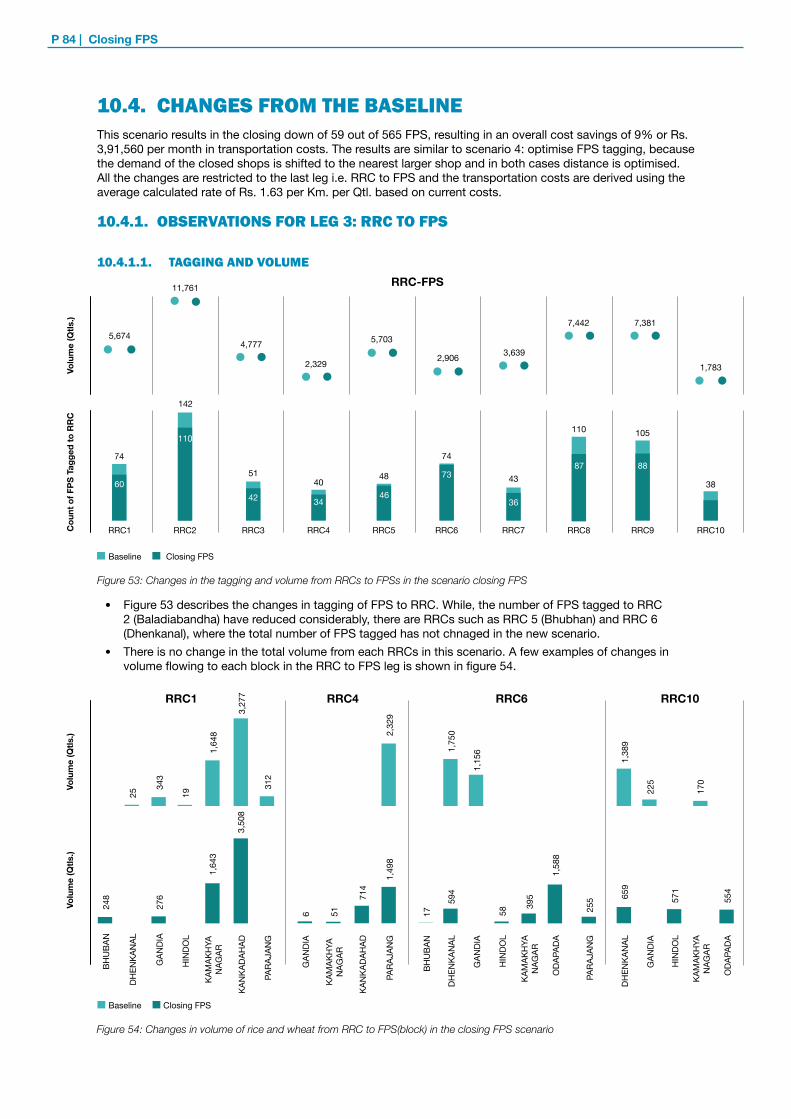
P 84 | Closing FPS
10.4. CHANGES FROM THE BASELINEThis scenario results in the closing down of 59 out of 565 FPS, resulting in an overall cost savings of 9% or Rs. 3,91,560 per month in transportation costs. The results are similar to scenario 4: optimise FPS tagging, because the demand of the closed shops is shifted to the nearest larger shop and in both cases distance is optimised. All the changes are restricted to the last leg i.e. RRC to FPS and the transportation costs are derived using the average calculated rate of Rs. 1.63 per Km. per Qtl. based on current costs.
10.4.1. OBSERVATIONS FOR LEG 3: RRC TO FPS
10.4.1.1. TAGGING AND VOLUME
• Figure 53 describes the changes in tagging of FPS to RRC. While, the number of FPS tagged to RRC 2 (Baladiabandha) have reduced considerably, there are RRCs such as RRC 5 (Bhubhan) and RRC 6 (Dhenkanal), where the total number of FPS tagged has not chnaged in the new scenario.
• There is no change in the total volume from each RRCs in this scenario. A few examples of changes in volume flowing to each block in the RRC to FPS leg is shown in figure 54.
Figure 53: Changes in the tagging and volume from RRCs to FPSs in the scenario closing FPS
Baseline Closing FPS
Cou
nt o
f FPS
Tag
ged
to R
RC
Volu
me
(Qtls
.)
RRC-FPS
RRC10
38
1,783
RRC9
105
7,381
88
RRC8
110
7,442
87
RRC7
43
3,639
36
RRC6
74
2,906
73
RRC5
48
5,703
46
RRC4
40
2,329
34
RRC3
51
4,777
42
RRC2
142
11,761
110
RRC1
74
5,674
60
Figure 54: Changes in volume of rice and wheat from RRC to FPS(block) in the closing FPS scenario
Volu
me
(Qtls
.)
RRC1 RRC4 RRC6 RRC10
Volu
me
(Qtls
.)
248
BHU
BAN
Baseline Closing FPS
25DH
ENKA
NAL
276
343
GAN
DIA
19H
INDO
L
11,
643
1,64
8KA
MAK
HYA
N
AGAR
3,50
83,
277
KAN
KADA
HAD
312
PARA
JAN
G
6G
ANDI
A
51KA
MAK
HYA
N
AGAR
714
KAN
KADA
HAD
1,49
82,
329
PARA
JAN
G
17BH
UBA
N
59
41,
750
DHEN
KAN
AL
1,15
6G
ANDI
A
58H
INDO
L
395
KAM
AKH
YA
NAG
AR
1,58
8O
DAPA
DA
255
PARA
JAN
G
659
1,38
9DH
ENKA
NAL
225
GAN
DIA
571
HIN
DOL
170
KAM
AKH
YA
NAG
AR
554
ODA
PADA

Optimisation of TPDS Supply Chain | P 85
10.4.1.2. DISTANCE AND COSTS
Figure 55, shows the average distance/Qtl and the cost of transportation for Leg 3 i.e. RRC to FPS. Overall the cost of transportation has reduced by 20% in this leg.
10.4.1.3. GEOSPATIAL REPRESENTATION OF THE SUPPLY CHAIN NETWORK IN THE CLOSING FPS SCENARIO
Geotagging from RRC to FPS for rice is described in Figure 56. As can be seen the tagging is optimised. For example, RRC2 was tagged to 142 FPS in the baseline; in the closing FPS scenario the tagging of FPS is reduced to 110 ensuring that movement of grains from east to west is reduced and that it is much more cohesive.
Figure 56: Geo-representation of tagging from RRC to FPS in the closing FPS scenario
RRC 1 RRC 2 RRC 3 RRC 4 RRC 5 RRC 6 RRC 7 RRC 8 RRC 9 RRC 10
Origin
BaselineRRC-FPS
Closing FPSRRC-FPS
Figure 55: Average distance travelled and total cost of transportation in the closing FPS scenario (Rice and Wheat)
Aver
age
Dis
tanc
e/Q
tl.
RRC-FPS
Cos
t of t
rans
port
atio
n (in
Rs.
Lak
h)
Baseline Closing FPS Leg Costs
RRC1
21.3017.40
1.9
1.6
RRC2
25.75
41.09
4.8
4.9
RRC4
12.46 15.09
0.7
0.6
RRC5
25.33
15.72
1.4
2.5
RRC6
18.11 16.77
1.2
0.8
RRC7
13.66 13.03
1.1
0.8
RRC8
12.7013.00
2.4
1.5
RRC9
18.7615.22
2.3
2.6
RRC10
14.6219.41
0.6 0.6
RRC3
16.8413.08
1.5
1.0

P 86 | Closing FPS
10.5. CHANGES REQUIRED TO IMPLEMENT THE SCENARIO POLICY CHANGES
• Classification of Supply Zones in the Food Security Rules and assigning of responsibilities.• Revision in the methodology for contracting of transporters including contracting terms, transportation rate
etc. to accommodate recommendation to move from per Qtl. rate to per Qtl. per Km. rate for the last leg i.e. RRC to FPS.
TECHNICAL CHANGE
• Changes to the SCMS and FPS Automation systems on tagging of nodes: i.e. tagging of RRC to FPS for allocation, movement and receipt of grains.
OPERATIONAL CHANGE
• Contracting of new Transport agents (L2 transporters) or changes to existing contracts to accommodate changes in rates of transportation, allocation and tagging.
• Preparation of new allocation orders based on the changes in tagging of RRC to FPS.• Close FPS which meet the constraint and are chosen to be closed by the optimisation model.• Changes in the planning/execution, delivery schedules and pick up of rice and wheat from RRC’s to FPS.

Optimisation of TPDS Supply Chain | P 87
11SCENARIO 8FULLY OPTISMISED WITH CAPACITY CONSTRAINT
CHAPTER

P 88 | Fully optimised with capacity constraint
11.1. ABOUT THE SCENARIOIn this scenario, the optimisation model assumes that the volume that travels between all nodes (PACS, Mill, RRC, FPS) can be changed, without any change in the total allocation to the node. This ensures that the impact on the individual locations is minimal. The efficiency gains in this scenario are based on optimising the tagging of the PACS to Mill, Mill to RRC and RRC to FPS legs simultaneously and changing the volumes that travel between these leg, without change in the total allocation at the final node. This scenario results in savings of 6% in leg 1, 17% in leg 2 and 19% in leg 3 which results in an overall saving of 14% or Rs. 6,34,096. For leg 3 i.e. RRC to FPS the costs are calculated using the average costs that were incurred in the baseline which is Rs. 1.63 per Qtl. per Km (refer table 9).
SCENARIO: BASELINE
SCENARIO: FULLY OPTIMISED WITH CAPACITY CONSTRAINT
TTC: Rs. 45,71,640 | ADT: 84 Km./Qtl. | ATC: 1.21 Rs. per Km./Qtl
TTC: Rs. 39,37,544 (-14%) | ADT: 73.3 Km./Qtl. | ATC: 1.24 Rs. per Km./Qtl.
**TTC - Total Transport Costs | ADT - Average Distance Travelled | ATC - Average Transportation Costs
11.2. KEY CONSTRIANTS1. All paddy that is procured is transported to one of the mills in the district.2. All paddy that is procured from the PACS is processed by the mills.3. All mills have an efficiency of 68%: for every Kg. of paddy that flows into the mill it produces exactly
0.68 Kg. of rice.4. All rice that is produced at the mills is transported to one of the 10 RRCs in Dhenkanal.5. All demand for rice and wheat at every FPS must be satisfied.6. All wheat demand in the district is fulfilled from FCI (Dhenkanal). 7. All volume flowing through the RRCs, Mills and FPS should remain the same as in the baseline.
Table 26: Summary statistics for fully optimised with capacity constraints scenario
SCENARIO 8. FULLY OPTIMISED WITH CAPACITY CONSTRAINT
Can be changed Remains the same Can be closed
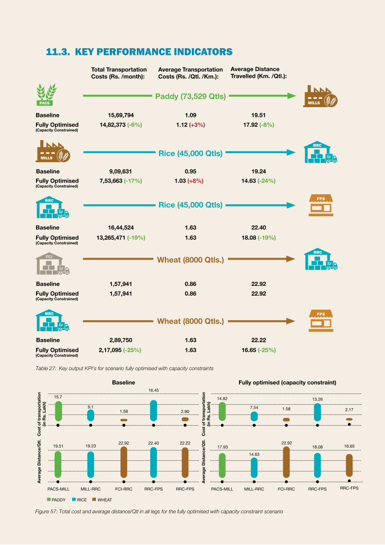
Optimisation of TPDS Supply Chain | P 89
Table 27: Key output KPI’s for scenario fully optimised with capacity constraints
Figure 57: Total cost and average distance/Qtl in all legs for the fully optimised with capacity constraint scenario
Baseline Fully optimised (capacity constraint)
Aver
age
Dis
tanc
e/Q
tl.
Aver
age
Dis
tanc
e/Q
tl.
Cos
t of t
rans
port
atio
n (in
Rs.
Lak
h)
Cos
t of t
rans
port
atio
n (in
Rs.
Lak
h)
15.7
19.51 19.23 22.92 22.40 22.22
14.82
17.9314.63
22.9218.08 16.65
7.549.11.58
16.45
2.90 1.58
13.26
2.17
PACS-MILL PACS-MILLMILL-RRC MILL-RRCFCI-RRC FCI-RRCRRC-FPS RRC-FPSRRC-FPS RRC-FPS
WHEATRICEPADDY
Baseline 15,69,794 1.09 19.5114,82,373 (-6%) 1.12 (+3%) 17.92 (-8%)Fully Optimised
(Capacity Constrained)
Baseline 0.95 19.249,09,6311.03 (+8%) 14.63 (-24%)7,53,663 (-17%)Fully Optimised
(Capacity Constrained)
Baseline 1.63 22.4016,44,524 1.63 18.08 (-19%)13,265,471 (-19%)Fully Optimised
(Capacity Constrained)
Baseline 1.63 22.222,89,7501.63 16.65 (-25%)2,17,095 (-25%)Fully Optimised
(Capacity Constrained)
Baseline 1,57,941 0.86 22.921,57,941 0.86 22.92Fully Optimised
(Capacity Constrained)
Wheat (8000 Qtls.)
Wheat (8000 Qtls.)
Rice (45,000 Qtls)
Rice (45,000 Qtls)
Paddy (73,529 Qtls)
11.3. KEY PERFORMANCE INDICATORSTotal Transportation Costs (Rs. /month):
Average Transportation Costs (Rs. /Qtl. /Km.):
Average Distance Travelled (Km. /Qtl.):
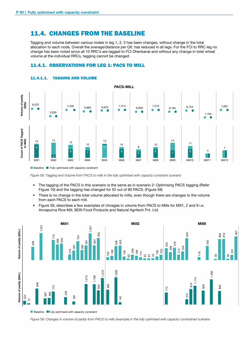
P 90 | Fully optimised with capacity constraint
11.4. CHANGES FROM THE BASELINETagging and volume between various nodes in leg 1, 2, 3 has been changes, without change in the total allocation to each node. Overall the average/distance per Qtl. has reduced in all legs. For the FCI to RRC leg no change has been noted since all 10 RRC’s are tagged to FCI Dhenkanal and without any change in total wheat volume at the individual RRCs, tagging cannot be changed.
11.4.1. OBSERVATIONS FOR LEG 1: PACS TO MILL
11.4.1.1. TAGGING AND VOLUME
• The tagging of the PACS in this scenario is the same as in scenario 2: Optimising PACS tagging (Refer Figure 16) and the tagging has changed for 52 out of 80 PACS. (Figure 58)
• There is no change in the total volume allocated to mills, even though there are changes to the volume from each PACS to each mill.
• Figure 59, describes a few examples of chnages in volume from PACS to Mills for Mill1, 2 and 9 i.e. Annapurna Rice Mill, BDN Food Products and Natural Agritech Pvt. Ltd.
Figure 58: Tagging and Volume from PACS to mills in the fully optimised with capacity constraint scenario
Volu
me
of p
addy
(Q
tls)
Cou
nt o
f PAC
S Ta
gged
to
Mill
s
Baseline Fully optimised with capacity constraint
Mill1
13 14 1210
1310 10
1411
47
7,097
1,764
6,7546,1847,212
6,0587,314
PACS-MILL
6,9755,9837,335
2,630
8,222
89
3
8 7
128 8 875
Mill2 Mill3 Mill4 Mill5 Mill6 Mill7 Mill8 Mill9 Mill10 Mill11 Mill12
Figure 59: Changes in volume of paddy from PACS to mills (example) in the fully optimised with capacity constrained scenario
0 0 0 0 0 0 0 0 0 0 0 0 0 0 0 0 0 0 0 0 0 0 0 0 0 0 0 0 0 0
00 0 0 0 000
66
0
500
1000
1500
2000
Volu
me
of p
addy
(Qtls
.)
224
Baseline Fully optimised with capacity constraint
74
948
367
390
773
439
182
1,21
5
1,19
884
21,
570
882
1,60
814
0
713
315
919 1,
114
829
1,49
0
805
907
201
5681
080
549
542
118
840
334
213
478
30845
3
204
139
7067676213
955
353
616
913
3
842
564
1,02
156
138
372
436
721
6
634
59977
3
1,03
1 Mill1 Mill2 Mill9
508
114168209
Volu
me
of p
addy
(Qtls
.)

Optimisation of TPDS Supply Chain | P 91
11.4.1.2. DISTANCE AND COSTS
Figure 60, describes the cost of transportation and the total distance between PACS and mills in the fully optimised with capacity constrained scenario. Cost of transportation for Mill 1 (Annapurna Rice Mills) and 12 (Tareni Agro Foods) has been increased since the average distance/Qtl. travelled from PACS to these mills has increased. For all other mills, the total cost of transportation has reduced.
11.4.2. OBSERVATIONS FOR LEG 2: MILL TO RRC
11.4.2.1. TAGGING AND VOLUME
• Tagging between mills to RRCs has been optimised, with number of nodes traversed reduced from 57 to 21. (Figure 61)
• This scenario is similar to optimise Leg 1 & 2 scenario, as an example, tagging of mills to RRC 6 has been reduced from 8 to1 in both scenario’s.
Figure 60: Average distance/Qtl. and cost of transportation from PACS to mills in the fully optimised with capacity constrained scenario
Aver
age
Dis
tanc
e/Q
tl.C
ost o
f tra
nspo
rtat
ion
( in
Rs.
Lak
h)
PACS-MILL
Baseline Fully optimised with capacity constraint
1.7
1.6
19.0821.93
Mill3
1.1 1.1
13.1614.63
Mill4
1.5 1.5
18.8717.91
Mill6
1.2 1.2
11.6612.08
Mill8
1.6
1.4
14.5920.85
Mill10
1.3
1.6
21.1313.83
Mill12
8.26
18.36
Mill11
0.4
0.3
19.02
29.08
Mill9
1.6
1.2
1.2
13.4217.86
Mill7
1.1
15.8022.92
Mill5
1.7
1.4
3.27
20.05
Mill2
0.5
0.2
36.08
23.85
Mill1
2.02.4
Leg Costs
Figure 61: Tagging and volume of rice from mills to RRC in the fully optimised with capacity constrained scenario
Baseline Fully optimised with capacity constraint
Cou
nt o
f Mill
s Ta
gged
to
each
RR
CVo
lum
e (Q
tls)
RRC1
5
2
5,207
RRC2
10
4
11,040
RRC3
31
4,750
RRC4
4
3
2,144
RRC5
4
2
5,020
MILL-RRC
RRC6
8
1
2,022
RRC7
5
1
3,639
RRC8
2
7,040
RRC9
9
4
7,547
RRC10
7
1
1,592

P 92 | Fully optimised with capacity constraint
11.4.2.2. DISTANCE AND COSTS
The cost of transportation has decreased for all nodes in the Mill to RRC leg, except for RRC 2 (Baladiabandha) and RRC 3 (Barihapur), because for these RRCs the average cost per Qtl. has increased.
(Please note: minor variations in costs may not be visible in the figure, since the costs are represented in lakh Rs.)
Figure 62: Changes in volume of rice from mills to RRC in the fully optimised with capacity constrained scenario
1 14
3,79
1
Volu
me
of R
ice
(Qtls
.)
MIL
L4
Baseline Fully optimised with capacity constraint
MIL
L7
1,08
7
238 70
7
1,19
9
3,63
9
1,59
2
230
124
146
14632
9
861
217
7601,
009
41
333
780
438
1,32
1
RRC1 RRC4 RRC7 RRC101,
554
1,11
3
52
2,18
0
248
248 45
0
MIL
L9
MIL
L9
MIL
L10
MIL
L10
MIL
L10
MIL
L11
MIL
L11
MIL
L12
MIL
L12
MIL
L3
MIL
L7
MIL
L7
MIL
L2
MIL
L4
MIL
L6
MIL
L8
MIL
L9
MIL
L10
MIL
L12
Volu
me
of R
ice
(Qtls
.)
Figure 63: Average distance/Qtl. and costs from mills to RRC in the in fully optimised with capacity constrained scenario
12.2
3
Aver
age
Dis
tanc
e/Q
tl.C
ost o
f tra
nspo
rtat
ion
(in R
s. L
akh)
26.64
6.25
28.55 29.69
14.23 14.65 13.389.53
25.35
16.75
27.29
3.77 5.392.70
5.97 5.81
18.51 16.15 17.64
10.51
RRC10RRC9RRC8RRC7RRC6RRC5RRC4RRC3RRC2RRC1
Baseline Leg costsFully optimised with capacity contraint
1.1
2.7 2.7
0.8 0.80.3
1.1
MILL-RRC
0.5 0.30.6 0.6
1.4
1.30.3
0.20.1 0.1
0.9
0.20.4
The total volume allocated to each RRC has not changed but the volume of rice between each mill and RRC has changed. Examples of the changes in volume between mills and RRC are shown in Figure 62.
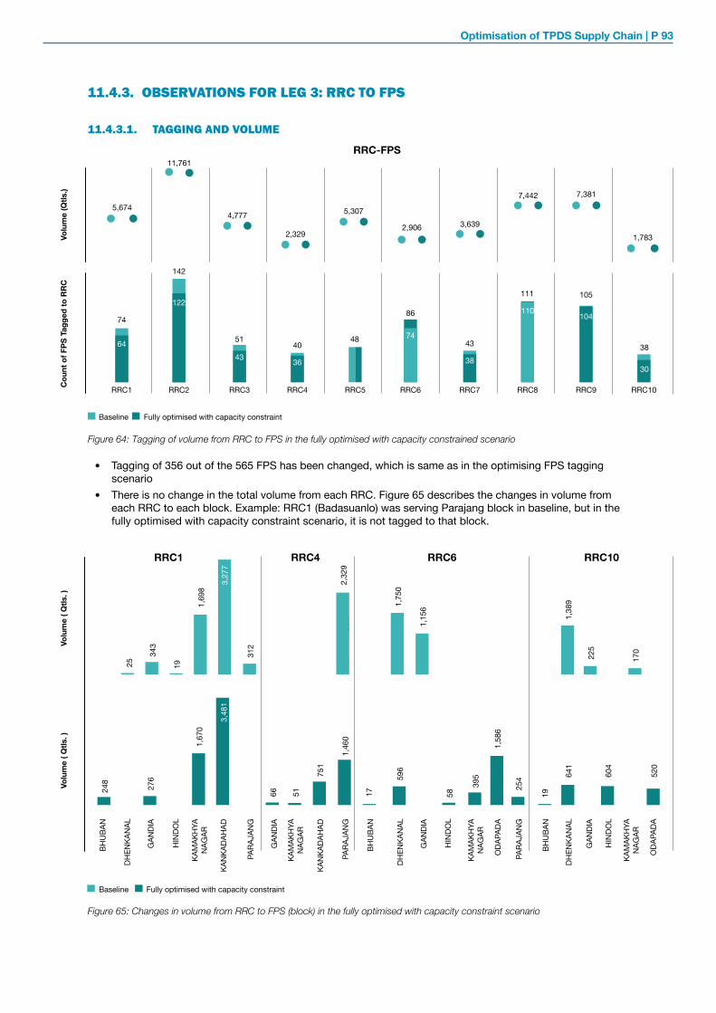
Optimisation of TPDS Supply Chain | P 93
11.4.3. OBSERVATIONS FOR LEG 3: RRC TO FPS
11.4.3.1. TAGGING AND VOLUME
• Tagging of 356 out of the 565 FPS has been changed, which is same as in the optimising FPS tagging scenario
• There is no change in the total volume from each RRC. Figure 65 describes the changes in volume from each RRC to each block. Example: RRC1 (Badasuanlo) was serving Parajang block in baseline, but in the fully optimised with capacity constraint scenario, it is not tagged to that block.
Figure 64: Tagging of volume from RRC to FPS in the fully optimised with capacity constrained scenario
Cou
nt o
f FPS
Tag
ged
to R
RC
Baseline
RRC1 RRC2 RRC3 RRC4 RRC5 RRC6 RRC7 RRC8 RRC9 RRC10
Fully optimised with capacity constraint
Volu
me
(Qtls
.)
38
105111
434051
74
5,674
11,761
4,777
2,329
5,307
RRC-FPS
2,906 3,639
7,442 7,381
1,783
142
43
122
64
86
48
104110
3836
74
30
Figure 65: Changes in volume from RRC to FPS (block) in the fully optimised with capacity constraint scenario
1 186
1
RRC1
248
276
1,67
0
66
3,48
1
Volu
me
( Qtls
. )Vo
lum
e ( Q
tls. )
RRC4 RRC6 RRC10
51 17
596
58 19
641
604
520
170
225
1,38
9
1,15
61,75
0
2,32
9
3,27
7
312
1,69
8
1925
343
395
1,58
6
25475
1
1,46
0
BHU
BAN
Baseline Fully optimised with capacity constraint
BHU
BAN
BHU
BAN
DHEN
KAN
AL
DHEN
KAN
AL
DHEN
KAN
AL
GAN
DIA
GAN
DIA
GAN
DIA
ODA
PADA
ODA
PADA
GAN
DIA
HIN
DOL
HIN
DOL
HIN
DOL
KAM
AKH
YA
NAG
AR
KAM
AKH
YA
NAG
AR
KAM
AKH
YA
NAG
AR
KAM
AKH
YA
NAG
AR
KAN
KADA
HAD
KAN
KADA
HAD
PARA
JAN
G
PARA
JAN
G
PARA
JAN
G

P 94 | Fully optimised with capacity constraint
11.4.3.2. DISTANCE AND COSTS
The total cost of transportation has reduced by 20% in leg 3 i.e RRC to FPS. The costs in this leg are calculated based on average cost per Qtl per Km. derived from the baseline costs.
11.4.4. GEOSPATIAL REPRESENTATION OF THE SUPPLY CHAIN NETWORK IN THE FULLY OPTIMISED WITH CAPACITY CONSTRAINED SCENARIO
Tagging between all nodes of the supply chain PACS to Mill, Mill to RRC, RRC to FPS has been optimised in this scenario. We can observe that the tagging from PACS to Mills is very similar to scenario 2: Optimising PACS tagging (refer figure 23), while the tagging from RRC to FPS is very similar to the optimising FPS tagging scenario (refer figure 38).
Figure 67: Geo-representation of tagging of PACS to mills in the fully optimised with capacity constrained scenario
BaselinePACS-MILL
Fully optimised with capacity constraintPACS-MILL
Figure 66: Average distance/Qtl. and cost of transportation from RRC to FPS in the fully optimised with capacity constrained scenario
Aver
age
Dis
tanc
e/Q
tl.C
ost o
f tra
nspo
rtat
ion
( in
Rs.
Lak
h)
RRC10
19.8514.62
RRC1
17.3421.30
1.9
1.6
RRC3
12.9416.84
1.5
1.0
RRC4
15.4612.46
0.7
0.6
RRC5
15.71
25.33
2.5
1.4
RRC9
18.7415.22
2.6
2.3
0.6 0.6
RRC8
12.8313.00
2.4
1.6
RRC6
16.1918.11
1.2
0.8
RRC7
13.0513.66
1.1
0.8
RRC2
25.82
41.09
4.8
5.0 RRC-FPS
Baseline Fully optimised with capacity constraint Leg costs
Mill 1 Mill 2 Mill 3 Mill 4 Mill 5 Mill 6 Mill 7 Mill 8 Mill 9 Mill 10 Mill 11 Mill 12
Destination

Optimisation of TPDS Supply Chain | P 95
Figure 69: Geo Representation of Tagging of RRC to FPS in the fully optimised with capacity constrained scenario
Figure 68: Geo-representation of tagging of mills to RRC in the fully optimised with capacity constrained scenario
BaselineMILL-RRC
BaselineRRC-FPS
Fully optimised with capacity constraint
Fully optimised with capacity constraint
MILL-RRC
RRC-FPS
RRC 1 RRC 2 RRC 3 RRC 4 RRC 5 RRC 6 RRC 7 RRC 8 RRC 9 RRC 10
Origin
RRC 1 RRC 2 RRC 3 RRC 4 RRC 5 RRC 6 RRC 7 RRC 8 RRC 9 RRC 10
Destination

P 96 | Fully optimised with capacity constraint
11.5. CHANGES REQUIRED TO IMPLEMENT THE SCENARIO POLICY CHANGES
• Classification of Supply Zones in the Food Security Rules and assigning of responsibilities.• Revision in the methodology for contracting of transporters including contracting terms, transportation rate
etc. to accommodate recommendation to move from per Qtl. rate to per Qtl. per Km. rate for the last leg i.e. RRC to FPS.
TECHNICAL CHANGE
• Changes to the SCMS and P-PAS databases on tagging of nodes: i.e. tagging of mills to RRCs and RRCs to FPS in SCMS and tagging of PACS to mills in the P-PAS system
OPERATIONAL CHANGE
• Contracting of new Transport agents (L1 and L2 transporters) or changes to existing contracts to accommodate changes in rates of transportation, allocation and tagging.
• Preparation of new allocation orders based on the changes in tagging of RRC to FPS.• Changes in the planning/execution, delivery schedules and pick up of paddy, rice and wheat between the
various nodes. 12

Optimisation of TPDS Supply Chain | P 97
12SCENARIO 9FULLY OPTISMISED WITH CAPACITY CONSTRAINT +15%
CHAPTER
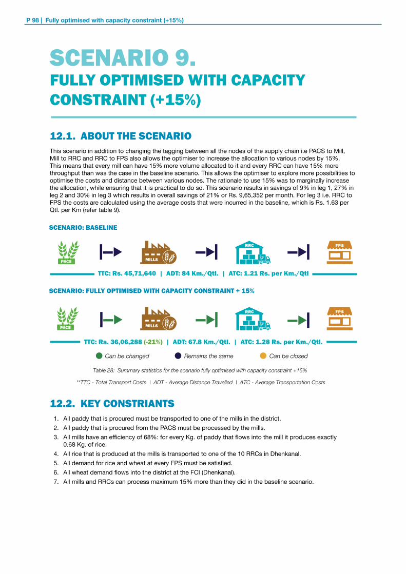
P 98 | Fully optimised with capacity constraint (+15%)
12.1. ABOUT THE SCENARIOThis scenario in addition to changing the tagging between all the nodes of the supply chain i.e PACS to Mill, Mill to RRC and RRC to FPS also allows the optimiser to increase the allocation to various nodes by 15%. This means that every mill can have 15% more volume allocated to it and every RRC can have 15% more throughput than was the case in the baseline scenario. This allows the optimiser to explore more possibilities to optimise the costs and distance between various nodes. The rationale to use 15% was to marginally increase the allocation, while ensuring that it is practical to do so. This scenario results in savings of 9% in leg 1, 27% in leg 2 and 30% in leg 3 which results in overall savings of 21% or Rs. 9,65,352 per month. For leg 3 i.e. RRC to FPS the costs are calculated using the average costs that were incurred in the baseline, which is Rs. 1.63 per Qtl. per Km (refer table 9).
SCENARIO: BASELINE
SCENARIO: FULLY OPTIMISED WITH CAPACITY CONSTRAINT + 15%
TTC: Rs. 45,71,640 | ADT: 84 Km./Qtl. | ATC: 1.21 Rs. per Km./Qtl
TTC: Rs. 36,06,288 (-21%) | ADT: 67.8 Km./Qtl. | ATC: 1.28 Rs. per Km./Qtl.
**TTC - Total Transport Costs | ADT - Average Distance Travelled | ATC - Average Transportation Costs
12.2. KEY CONSTRIANTS1. All paddy that is procured must be transported to one of the mills in the district.2. All paddy that is procured from the PACS must be processed by the mills. 3. All mills have an efficiency of 68%: for every Kg. of paddy that flows into the mill it produces exactly
0.68 Kg. of rice.4. All rice that is produced at the mills is transported to one of the 10 RRCs in Dhenkanal.5. All demand for rice and wheat at every FPS must be satisfied.6. All wheat demand flows into the district at the FCI (Dhenkanal).7. All mills and RRCs can process maximum 15% more than they did in the baseline scenario.
Table 28: Summary statistics for the scenario fully optimised with capacity constraint +15%
SCENARIO 9. FULLY OPTIMISED WITH CAPACITY CONSTRAINT (+15%)
Can be changed Remains the same Can be closed
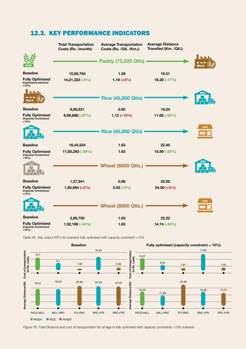
Optimisation of TPDS Supply Chain | P 99
15,69,794 1.09 19.5114,21,323 (-9%) 1.19 (+9%) 16.20 (-17%)
0.95 19.249,09,6311.12 (+18%) 11.82 (-39%)6,66,888 (-27%)
1.63 22.4016,44,524 1.63 15.89 (-29%)11,65,293 (-29%)
1.63 22.222,89,7501.63 14.74 (-34%)1,92,198 (-34%)
Table 29: Key output KPI’s for scenario fully optimised with capacity constraint +15%
Figure 70: Total Distance and cost of transportation for all legs in fully optimised with capacity constraints +15% scenario
1,57,941 0.86 22.921,60,584 (+2%) 0.83 (-3%) 24.09 (+5%)
WHEATRICEPADDY
PACS-MILL MILL-RRC FCI-RRC RRC-FPS RRC-FPS
Aver
age
Dis
tanc
e/Q
tl.C
ost o
f tra
nspo
rtat
ion
(in R
s. L
akh)
15.7
9.11.58
16.45
2.90
19.51 19.24 22.92 22.40 22.22
PACS-MILL MILL-RRC FCI-RRC RRC-FPS RRC-FPS
Aver
age
Dis
tanc
e/Q
tl.C
ost o
f tra
nspo
rtat
ion
(in R
s. L
akh) 14.21
16.2011.82
24.09
15.89
6.671.61
11.65
1.92
14.74
Baseline Fully optimised (capacity constraint + 15%)
BaselineFully Optimised (CapacityConstrained +15%)
BaselineFully Optimised (Capacity Constrained +15%)
BaselineFully Optimised (Capacity Constrained +15%)
BaselineFully Optimised (Capacity Constrained +15%)
BaselineFully Optimised (Capacity Constrained +15%)
Paddy (73,529 Qtls)
Rice (45,000 Qtls)
Wheat (8000 Qtls.)
Rice (45,000 Qtls)
Wheat (8000 Qtls.)
12.3. KEY PERFORMANCE INDICATORSTotal Transportation Costs (Rs. /month):
Average Transportation Costs (Rs. /Qtl. /Km.):
Average Distance Travelled (Km. /Qtl.):

P 100 | Fully optimised with capacity constraint (+15%)
12.4. CHANGES FROM THE BASELINE In the optimal configuration of this scenario the tagging of 53 out of 80 PACS changes and the tagging of 305 out of 565 FPS changes. This results in a cost decrease of 9% in leg 1, 27% in leg 2 and 30% in leg 3 but a 2% increase in costs in the FCI to RRC leg. This is because with the optimisation under the given constraints the average cost/Qtl has decreased for all other legs except the FCI to RRC leg.
12.4.1. OBSERVATIONS FOR LEG 1: PACS TO MILL
12.4.1.1. TAGGING AND VOLUME
• Tagging of PACS to mills has been changed. The number of nodes traversed had reduced for 125 to 75.• The allocation to each mill has been increased by 15%. Figure 71 describes the changes in tagging and
volume of paddy allocated to each mill in comparison to the baseline.
12.4.1.2. DISTANCE AND COSTS
Costs and distance travelled are aligned to the changes in the allocation and tagging of PACS to Mill. Distance between PACS and mills have significantly reduced for all mills except for Mill 5 (Kamlesh Rice Mill) and Mill 12 (Tareni Agro Foods), where the tagging and average distance/Qtl. has increased.
Figure 71: Tagging and volume of paddy from PACS to mills in the fully optimised with capacity constraint +15% scenario
Cou
nt o
f PAC
S Ta
gged
to
Mill
sVo
lum
e of
pad
dy
( Qtls
. )
Mill11
4
1,764
2,028
Mill12
7
7,097
8,162
Mill8
10
7,212
8,294
Mill6
10
7,314
8,411
6,058
6,967
Mill7
8
6
6,975
8,022
Mill5
15
12
5,983
6,881
Mill4
10
9
Mill3
12
7,335
4,661
6
Mill2
14
2,630
3,024
3
8,222
3,885
Mill1
13
5
6,754
7,003
Mill10
11
7
6,184
6,191
Mill9
14
8
Baseline Fully optimised with capacity constraint (+15%)
PACS-MILL
Figure 72: Cost of transportation and distance travelled from PACS to mills in the fully optimised with capacity constraint +15% scenario
Aver
age
Dis
tanc
e/Q
tl.C
ost o
f tra
nspo
rtat
ion
(in R
s. L
akh)
PACS-MILL
2.0
0.7
15.66
23.85
Mill1
Baseline Fully optimised with capacity constraint (+15%) Leg costs
0.5
0.2
20.05
4.02
Mill2
1.7
0.8
13.00
21.93
Mill3
1.1
1.3
13.7514.63
Mill4
1.7
1.8
19.5322.92
Mill5
1.5
1.8
19.3817.91
Mill6
17.8616.39
1.3
1.2
Mill7
1.4
1.2
12.3512.08
Mill8
1.6
1.2
18.70
29.08
Mill9
1.5
1.6
18.2020.85
Mill10
67
0.4
0.3
7.15
18.36
Mill11
1.3
1.8
20.7013.83
Mill12

Optimisation of TPDS Supply Chain | P 101
12.4.2. OBSERVATIONS FOR LEG 2: MILL TO RRC AND FCI TO RRC
12.4.2.1. TAGGING AND VOLUME
• Tagging of Mill to RRC as well as the allocation of rice to RRCs has been changed in this scenario. Figure 73 describes the changes in tagging and allocation of each RRC.
• Except for RRC 2, the allocation for all RRC,s have been increased by about 15% of its existing allocation.• The number of nodes traversed have reduced from 57 to 19.• Figure 74, describes the changes in allocation of wheat between FCI and RRC in comparison to baseline. • Tagging for FCI-RRC remains 1 to 1 as in the baseline, but allocation of wheat has been increased for all
RRCs except RRC 2.
Figure 73: Tagging and allocation of rice from mills to RRCs in the fully optimised with capacity constraints +15% scenario
Cou
nt o
f Mill
s Ta
gged
to
eac
h R
RC
Volu
me
(Qtls
.)
1,592
1,830
1
7
RRC10
7,547
8,679
3
9
RRC9
7,040
8,096
2
RRC8
3,639
4,185
1
5
RRC7
2,022
2,326
1
8
RRC6
5,020
5,773
24
RRC5
2,144
2,466
24
RRC4
4,750
5,463
23
RRC3
11,040
5,196
10
3RRC2
5,207
5,988
5
2RRC1
Baseline Fully optimised with capacity constraint(+15%)
MILL-RRC
Figure 74: Tagging and allocation of wheat from FCI to RRCs in the fully optimised with capacity constraints +15% scenario
Cou
nt o
f FC
I w
areh
ouse
to R
RC
RRC4
1
399
459
RRC5
1
789
907
RRC6
1
1,086
1,249
RRC7
1
364
417
RRC10
1
351
404
RRC9
1
589
677
RRC8
1
1,106
1,272
RRC3
1
502
577
1
RRC1
988
1,137
RRC2
1
899
1,825
FCI-RRC
Baseline Fully optimised with capacity constraint(+15%)
Volu
me
of R
ice
(Qtls
.)

P 102 | Fully optimised with capacity constraint (+15%)
12.4.2.2. DISTANCE AND COSTS
• The distance and cost of transportation has reduced for most RRCs. For RRC 9 even though average distance/Qtl. has reduced, the cost of transportation has increased because the total volume allocated to the RRC has increased. Similarly for RRC 2, the cost of transportation has decreased significantly, since the volume allocated to the RRC as well as the average distance/Qtl. has dropped.
• The distance between mills and RRCs have significantly reduced resulting in cost reduction of 27%.
Figure 75: Cost of transportation and distance from mills to RRC in the fully optimised with capacity constraint +15% scenario
Aver
age
Dis
tanc
e/Q
tl.C
ost o
f tra
nspo
rtat
ion
(in R
s. L
akh)
MILL-RRC
2.7
1.1
21.20
28.55
RRC2
1.1
0.8
18.8614.23
RRC3
0.3
0.2
9.4313.38
RRC4
1.1 1.1
16.75
25.35
RRC5
0.5
0.1
3.77
27.29
RRC6
0.3
0.2
5.392.70
RRC7
0.6
0.7
5.815.97
RRC8
1.4
1.5
15.4318.51
RRC9
0.3 0.3
10.51
17.64
RRC10
1.1
0.4
RRC1
6.25
26.64
Baseline Fully optimised with capacity constraint (+15%) Leg costs
Figure 76: Cost of transportation and distance from FCI to RRC in the fully optimised with capacity constraint +15% scenario
Baseline Leg costsFully optimised with capacity constraint (+15%)
37.29
RRC1
28,309
32,556
RRC2
15.08
32,013
15,767
RRC6
0
0 0
RRC7
10.23
5,508
6,334
RRC10
7.81
4,111
4,728
RRC9
7.77
6,863
7,892
RRC8
30.50
27,925
32,114
RRC5
49.03
26,511
30,487
RRC4
36.79
11,339
13,040
RRC3
41.48
15,362
17,666
FCI-RRC
Aver
age
Dis
tanc
e/Q
tl.C
ost o
f tra
nspo
rtat
ion
(in R
s. L
akh)
The distance travelled from FCI to RRC, shows no change, but due to the changes in the volume of wheat from FCI to each RRC, the costs have changed. Overall, the cost has increased by 2%.
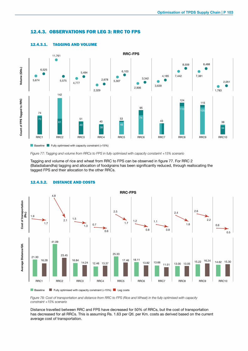
Optimisation of TPDS Supply Chain | P 103
12.4.3. OBSERVATIONS FOR LEG 3: RRC TO FPS
12.4.3.1. TAGGING AND VOLUME
Tagging and volume of rice and wheat from RRC to FPS can be observed in figure 77. For RRC 2 (Baladiabandha) tagging and allocation of foodgrains has been significantly reduced, through reallocating the tagged FPS and their allocation to the other RRCs.
12.4.3.2. DISTANCE AND COSTS
Distance travelled between RRC and FPS have decreased for 50% of RRCs, but the cost of transportation has decreased for all RRCs. This is assuming Rs. 1.63 per Qtl. per Km. costs as derived based on the current average cost of transportation.
Figure 77: Tagging and volume from RRCs to FPS in fully optimised with capacity constarint +15% scenario
Cou
nt o
f FPS
Tag
ged
to R
RC
74
5,674
6,525
11,761
5,5754,777
5,494
2,329
2,678
6,103
RRC-FPS
142
5140
53
95
437061
4938
48
74
110 105
34
Volu
me
(Qtls
.)
124115
38
5,307
2,906
3,342
3,639
4,185 7,442 7,381
1,783
2,051
8,4888,559
RRC1
Baseline Fully optimised with capacity constraint (+15%)
RRC2 RRC3 RRC4 RRC5 RRC6 RRC7 RRC8 RRC9 RRC10
Figure 78: Cost of transportation and distance from RRC to FPS (Rice and Wheat) in the fully optimised with capacity constraint +15% scenario
Aver
age
Dis
tanc
e/Q
tl.C
ost o
f tra
nspo
rtat
ion
(Rs.
)
14.62 15.30
0.6
0.5
RRC10
15.22 16.24
2.6
2.2
RRC9
13.00 13.05
1.8
2.4
RRC8
13.6611.51
0.8
1.1
RRC7
1.2
0.8
18.1113.82
RRC6
2.5
1.7
25.33
17.46
RRC5
0.7
0.6
12.46 13.37
RRC4
1.5
1.3
16.8414.24
RRC3
4.8
2.1
41.09
23.45
RRC2
21.3016.28
1.9
1.7
RRC1
Baseline Fully optimised with capacity constraint (+15%) Leg costs
RRC-FPS

P 104 | Fully optimised with capacity constraint (+15%)
12.4.4. GEOSPATIAL REPRESENTATION OF THE SUPPLY CHAIN NETWORK IN THE FULLY OPTIMISED WITH CAPACITY CONSTRAINED +15% SCENARIO
Figure 79-81 describe the geo tagging of nodes for each leg in this scenario. The tagging in all legs is very similar, but more optimised than the scenario fully optimised with capacity constrained. There is no change in tagging from FCI to RRC, hence geo-representation for that leg is not included.
Figure 79: Geo-representation of tagging from PACS to Mills in fully optimised with capacity constarints +15% scenario
Figure 80: Geo-representation of tagging from Mills to RRC in the fully optimised with capacity constarint +15% scenario
Mill 1 Mill 2 Mill 3 Mill 4 Mill 5 Mill 6 Mill 7 Mill 8 Mill 9 Mill 10 Mill 11 Mill 12
Destination
Fully optimised with capacity constraint +15%PACS-MILL
MILL-RRC
BaselinePACS-MILL
BaselineMILL-RRC
Fully optimised with capacity constraint +15%
RRC 1 RRC 2 RRC 3 RRC 4 RRC 5 RRC 6 RRC 7 RRC 8 RRC 9 RRC 10
Destination
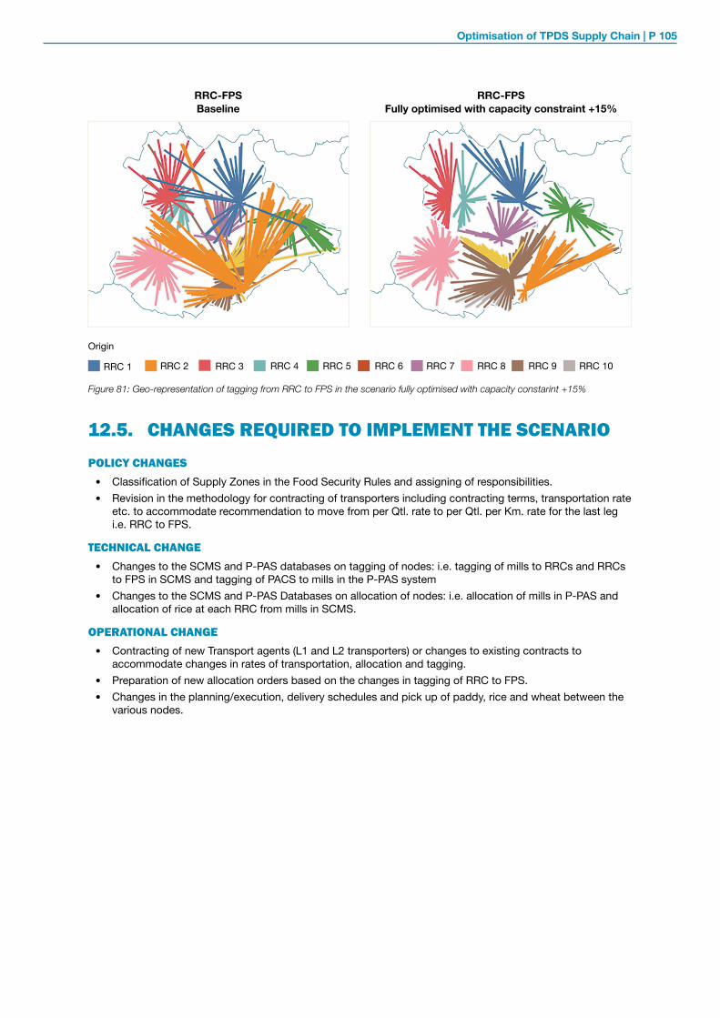
Optimisation of TPDS Supply Chain | P 105
Figure 81: Geo-representation of tagging from RRC to FPS in the scenario fully optimised with capacity constarint +15%
12.5. CHANGES REQUIRED TO IMPLEMENT THE SCENARIO POLICY CHANGES
• Classification of Supply Zones in the Food Security Rules and assigning of responsibilities.• Revision in the methodology for contracting of transporters including contracting terms, transportation rate
etc. to accommodate recommendation to move from per Qtl. rate to per Qtl. per Km. rate for the last leg i.e. RRC to FPS.
TECHNICAL CHANGE
• Changes to the SCMS and P-PAS databases on tagging of nodes: i.e. tagging of mills to RRCs and RRCs to FPS in SCMS and tagging of PACS to mills in the P-PAS system
• Changes to the SCMS and P-PAS Databases on allocation of nodes: i.e. allocation of mills in P-PAS and allocation of rice at each RRC from mills in SCMS.
OPERATIONAL CHANGE
• Contracting of new Transport agents (L1 and L2 transporters) or changes to existing contracts to accommodate changes in rates of transportation, allocation and tagging.
• Preparation of new allocation orders based on the changes in tagging of RRC to FPS.• Changes in the planning/execution, delivery schedules and pick up of paddy, rice and wheat between the
various nodes.
RRC-FPSFully optimised with capacity constraint +15%Baseline
RRC-FPS
RRC 1 RRC 2 RRC 3 RRC 4 RRC 5 RRC 6 RRC 7 RRC 8 RRC 9 RRC 10
Origin
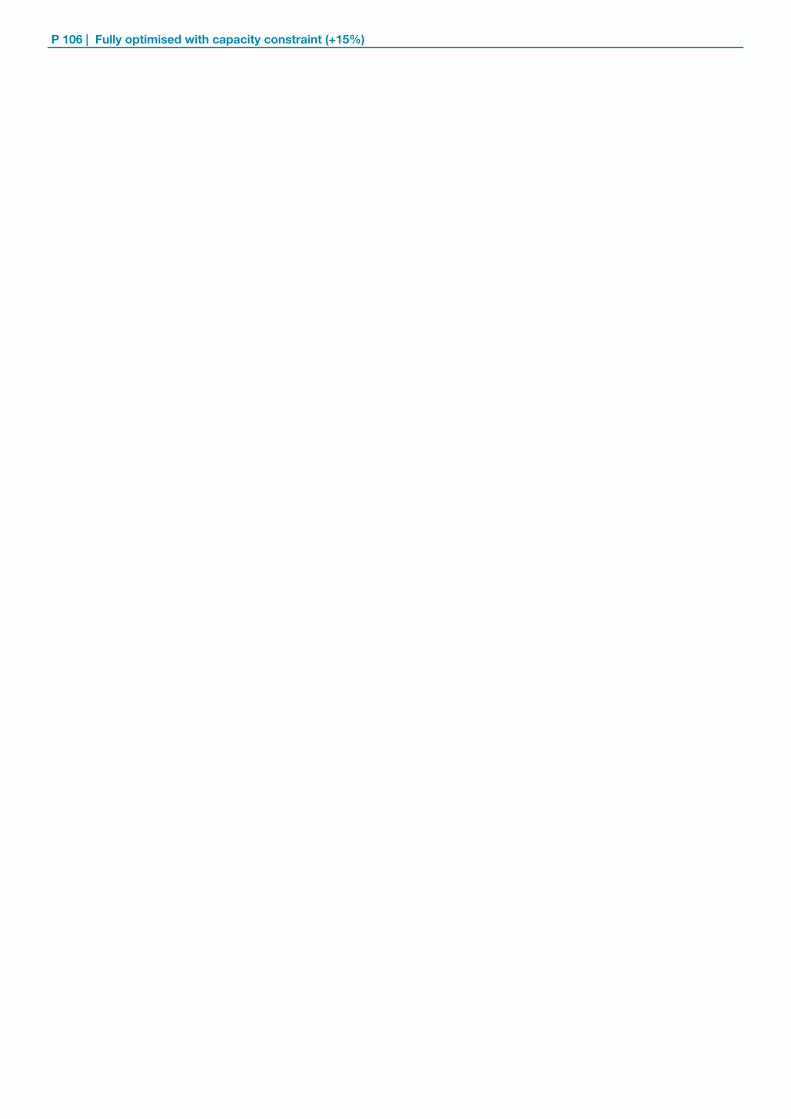
P 106 | Fully optimised with capacity constraint (+15%)
13

Optimisation of TPDS Supply Chain | P 107
13SCENARIO 10FULLY OPTISMISED
CHAPTER

P 108 | Fully optimised
13.1. ABOUT THE SCENARIOIn this scenario, the optimisation model chooses to change the tagging and allocated volume in all the three legs i.e PACS to Mill, Mill to RRC, FCI to RRC and RRC to FPS, as long as all the procured paddy picked up from the PACS and the demand of rice, wheat is fulfilled at the FPSs. This scenario thus provides insight on the changes that could potentially be made in the network to maximise the cost savings, while ensuring that it is practical to implement. The change in throughput of the different locations i.e mills, RRCs as compared to the baseline provides information about what locations should be expanded or reduced to minimise the costs of transportation. Overall, the costs savings in this scenario is 29% or Rs.13,23,474, with cost savings of 13%, 50% and 32% in leg 1, 2 and 3 respectively.
SCENARIO: BASELINE
SCENARIO: FULLY OPTIMISED
TTC: Rs. 45,71,640 | ADT: 84 Km./Qtl. | ATC: 1.21 Rs. per Km./Qtl
TTC: Rs. 32,48,206 (-29%) | ADT: 54.9 Km./Qtl. | ATC: 1.37 Rs. per Km./Qtl.
**TTC - Total Transport Costs | ADT - Average Distance Travelled | ATC - Average Transportation Costs
13.2. KEY CONSTRIANTS1. All paddy that is procured must be transported to one of the mills in the district.2. All paddy that is procured from the PACS must be processed by the mills. 3. All mills have an efficiency of 68%: for every Kg. of paddy that flows into the mill it produces exactly 0.68
Kg. of rice.4. All rice that is produced at the mills is transported to one of the 10 RRCs in Dhenkanal.5. All demand for rice and wheat at every FPS must be satisfied.6. All wheat demand flows into the district at the FCI (Dhenkanal).
Table 30: Summary statistics for the fully optimised scenario
SCENARIO 10. FULLY OPTIMISED
Can be changed Remains the same Can be closed

Optimisation of TPDS Supply Chain | P 109
15,69,794 1.09 19.5113,58,835 (-13%) 1.26 (+16%) 14.57 (-25%)
0.95 19.249,09,6311.31 (+37%) 6.96 (-64%)4,55,514 (-50%)
1.63 22.4016,44,524 1.63 15.13 (-32%)11,09,461 (-33%)
1.63 22.222,89,7501.63 15.87 (-29%)2,06,881 (-29%)
Figure 82: Total cost of transportation and average distance/Qtl. in all legs for the fully optimised scenario
1,57,941 0.86 22.92
1,17,514 (-26%) 0.81 (-7%) 18.22 (-21%)
WHEATRICEPADDY
PACS-MILL PACS-MILLMILL-RRC MILL-RRCFCI-RRC FCI-RRCRRC-FPS RRC-FPSRRC-FPS RRC-FPS
Aver
age
Dis
tanc
e/Q
tl.
Aver
age
Dis
tanc
e/Q
tl.
Cos
t of t
rans
port
atio
n (in
Rs.
Lak
h)
Cos
t of t
rans
port
atio
n (in
Rs.
Lak
h)
15.7
9.11.58
16.45
13.59
14.5718.22
15.13 15.87
6.96
4.56
11.09
2.071.18
2.90
19.51 19.24 22.92 22.40 22.22
Baseline Fully optimised
13.3. KEY PERFORMANCE INDICATORS
Baseline
Total Transportation Costs (Rs. /month):
Average Transportation Costs (Rs. /Qtl. /Km.):
Average Distance Travelled (Km. /Qtl.):
Fully Optimised
BaselineFully Optimised
BaselineFully Optimised
BaselineFully Optimised
Baseline
Fully Optimised
Paddy (73,529 Qtls)
Rice (45,000 Qtls)
Rice (45,000 Qtls)
Wheat (8000 Qtls.)
Wheat (8000 Qtls.)
Table 31: Key output KPI’s for the fully optimised scenario

P 110 | Fully optimised
13.4. CHANGES FROM THE BASELINEIn this scenario, the tagging and throughput of all nodes of the supply chain have been changes, keeping the total procurement at PACS and distribution at FPS same as the baseline. Overall, the cost of transportation and average distance/Qtl. has reduced in all legs of the supply chain.
13.4.1. OBSERVATIONS FOR LEG 1: PACS TO MILL
13.4.1.1. TAGGING AND VOLUME
• The number of PACS tagged to each mill has been changed, without any change in total quantity of paddy picked from each PACS or the total number of PACS.
• The number of nodes traversed in this leg have reduced from 125 to 82.• The quantity of paddy processed by each mill has changed, without any change in the total quantity
of paddy processed by all mills. Figure 83, describes the change in volume processed by each mill as compared to the baseline.
• These changes have led to an overall reduction of 13% in total transportation costs.• Mill 10 (Panchasakha Rice Mill) has not been tagged to any PACS in the fully optimised scenario.
13.4.1.2. DISTANCE AND COSTS
Figure 83: Tagging and volume of paddy from PACS to mills in the fully optimised scenario
Cou
nt o
f PAC
S Ta
gged
to
Mill
sVo
lum
e of
pad
dy
(Qtls
.)
6,754
11
Mill10
7,314
8,050
10
Mill6
1,821
5,983
2
10
Mill4
1,345
7,335
2
12
Mill3
2,630
6,847
5
14
Mill2
8,222
2,040
13
2Mill1
Baseline Fully optimised
6,975
10,709
Mill5
17
12
6,058
13,315
12
Mill7
8
11,955
7,212
13
Mill8
10
6,184
1,872
14
Mill92
1,764
10,429
12
Mill11
4
7,097
5,147
7
Mill12
5
PACS-MILL
Figure 84: Cost of transportation and average distance/Qtl for PACS to mills in the fully optimised scenario
Baseline Fully optimised Leg costs
Cos
t of t
rans
port
atio
n (in
Rs.
lakh
)Av
erag
e D
ista
nce/
Qtl.
0.3
2.0
23.85
7.67
Mill1
20.05
9.55
Mill2
0.5
1.0
21.93
6.10
Mill3
0.1
1.7
14.63
6.48
Mill4
0.2
1.1
Mill6
17.91 17.78
1.5
1.6
29.08
18.09
Mill9
0.3
1.6
20.85
Mill10
1.6
18.36 17.37
Mill11
0.4
2.2
13.83 11.60
Mill12
0.8
1.3
Mill8
12.08 13.12
1.2
2.2
Mill7
17.8614.06
1.2
2.5
Mill5
22.9219.43
1.7
2.4
PACS-MILL

Optimisation of TPDS Supply Chain | P 111
The average distance/Qtl. has reduced by 25% and cost of transportation by 13% in the PACS to Mill leg for the fully optimised scenario. For 50% of the mills i.e Mill 2,5,6,7,8,11, the cost of transportation has gone up, since the volume of paddy allocated to these mills has gone up.
13.4.2. OBSERVATIONS FOR LEG 2: MILL TO RRC AND FCI TO RRC
13.4.2.1. TAGGING AND VOLUME
• The number of mills tagged to each RRC has been optimised, with the number of nodes traversed reduced from 57 to 15.
• The allocation of RRC 2,3,9 and 10 has been decreased, while for all other RRC’s the total allocation has increased.
• FCI Dhenkanal (RRC6) stores wheat which is then transported to other RRCs. In all other scenarios’ FCI Dhenkanal is tagged to all the RRCs, but in this scenario RRC 9 and 10 no longer receive wheat from FCI (Figure 86).
• Total allocation to RRC 6 has been trippled, while for RRC2 it has been reduced to 5% of its allocation in baseline (Figure 86).
• This overall quantity of wheat procured from FCI as well as wheat delivered to individual FPSs for distribution to beneficiaries has not been changed.
Figure 85: Tagging and volume of rice from mills to RRC in the fully optimised scenario
Baseline Fully optimised
MILL-RRC
Cou
nt o
f Mill
s Ta
gged
to
RR
CVo
lum
e (Q
tls.)
RRC1
5,207
9,054
5
1
11,040
724
2
10
RRC2
4,750
4,068
23
RRC3
2,144
3,938
1
4
RRC4
5,020
7,528
1
4
RRC5
2,022
5,474
1
8
RRC6
8
3,639
4,773
2
5
RRC7
7,040
8,737
23
RRC8
7,547
4,656
1
9
RRC9
1,592
994
1
7
RRC10
Figure 86: Volume of wheat from FCI to RRC
Baseline Fully optimised
Volu
me
of W
heat
(Qtls
.)
FCI-RRC
RRC100
351
RRC90
589
RRC8
1,2881,106
RRC7
788364
RRC6
3,479
1,089
RRC5
500789
RRC4
279399
RRC3
778502
RRC2
79
1,825
RRC1
809988
13.4.3. DISTANCE AND COSTS
• Overall, as described in Figure 87, 88 the total cost and average distance/Qtl. has reduced considerably in leg 2 i.e. Mill to RRC and RRC to FCI in the fully optimised scenario.
• For RRC 6 the distance travelled and cost of transportation is zero since FCI Dhenkanal and RRC 6 is same. Since RRC 9 and 10 are not allocated any wheat, the costs in the fully optimised scenario for these RRCs is zero.
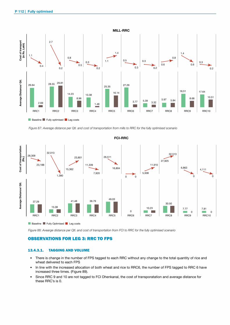
P 112 | Fully optimised
OBSERVATIONS FOR LEG 3: RRC TO FPS
13.4.3.1. TAGGING AND VOLUME
• There is change in the number of FPS tagged to each RRC without any change to the total quantity of rice and wheat delivered to each FPS
• In line with the increased allocation of both wheat and rice to RRC6, the number of FPS tagged to RRC 6 have increased three times. (Figure 89).
• Since RRC 9 and 10 are not tagged to FCI Dhenkanal, the cost of transporatation and average distance for these RRC’s is 0.
Figure 87: Average distance per Qtl. and cost of transportation from mills to RRC for the fully optimised scenario
Aver
age
Dis
tanc
e/ Q
tl.C
ost o
f tra
nspo
rt
(in R
s. L
akh)
MILL-RRC
Baseline Fully optimised Leg costs
25.35
16.14
1.4
1.1
RRC5
27.29
3.77
0.3
0.5
RRC6
17.64
10.51
0.2
0.3
RRC10RRC1
26.64
2.69
1.1
0.4
28.55 29.81
RRC2
2.7
0.2
14.238.96
RRC3
0.8
0.5
13.38
1.48
RRC4
0.3
0.2
5.39 3.32
RRC7
0.3
0.2
18,51
8.68
RRC9
0.6
1.4
5.97 5.84
RRC8
0.6
0.8
Figure 88: Avearge distance per Qtl. and cost of transportation from FCI to RRC for the fully optimised scenario
Cos
t of t
rans
port
atio
n (R
s.)
Aver
age
Dis
tanc
e/ Q
tl.
37.29
28,309
23,188
RRC1 RRC4
36.79
11,339
7,920
FCI-RRC
RRC5
49.03
26,511
16,804
RRC7
10.23
5,508
11,910
RRC9
7.77
6,863
0
RRC10
7.81
0
4,111
RRC8
30.50
27,925
32,513
RRC60
0 0
RRC3
41.48
15,362
23,801
RRC2
15.08
32,013
1,380
Baseline Fully Optimised Leg costs
0 0

Optimisation of TPDS Supply Chain | P 113
13.4.3.2. DISTANCE AND COSTS
• For RRC 1, even though the average distance per Qtl. has reduced, the tagging and volume of rice from RRC to FPS has increased, hence the costs have increased.
• As tagging and allocation to RRC 2 (Baladiabandha) has been reduced significantly, the average distance/Qtl. and cost of transportation has also reduced significantly. Overall the reduction in total costs in this leg is 32%. (Figure 90).
Figure 90: Cost of transportation and average distance per Qtl. of RRC to FPS in the fully optimised scenario
20.0
5
Cos
t of t
rans
port
atio
n (in
Rs.
Lak
h)Av
erag
e D
ista
nce/
Qtl.
21.30
1.9
2.4
4.8
16.32
41.09
4.27
16.8412.25 12.46
17.6225.33
21.3418.11 15.00 13.66 13.00 13.07 15.22 15.01 14.62
8.42
RRC10RRC9RRC8RRC7RRC6RRC5RRC4RRC3RRC2RRC1
Baseline Fully optimised Leg costs
12.61
0.1
1.5
0.9 0.7
1.1
2.5 2.5
RRC-FPS
1.2
2.1
1.1
1.0
2.4 2.6
1.00.6
0.1
1.9
13.4.4. GEOSPATIAL REPRESENTATION OF THE SUPPLY CHAIN NETWORK IN THE FULLY OPTIMISED
• Overall figures 91-94 describe the tagging of nodes in all legs i.e. PACS to Mill, Mill to RRC, FCI to RRC and RRC to FPS. It can be observed that the tagging is optimised for all the legs leading to reduction in distance and cost of transportation.
• Tagging from mills to RRC has been further optimised from scenario 8 and 9. As can be seen, number of mills tagged to RRCs have reduced considerably, with maximum reduction in tagging for RRC2 (Baladiabandha). (Figure 92)
• Figure 93, shows the tagging from FCI to RRC. As can be seen, RRC9 and 10 are not tagged to FCI in the fully optimised scenario.
• Figure 94, represents the tagging between RRC to FPS for rice. As can be seen, the tagging has been optimised by supply zone thereby reducing the overall distance and costs in each leg 13.4.
Figure 89: Tagging and volume of rice and wheat from RRC to FPS
Cou
nt o
f FPS
Tag
ged
to R
RC
Volu
me
(Qtls
.)
Baseline
RRC1
749 51 40 48 43 56
11
11076
142
5941
72 79
138105
38
894
1,7834,190
7,3819,151
7,4425,084
3,639
74
RRC2 RRC3 RRC4 RRC5 RRC6 RRC7 RRC8 RRC9 RRC10
Fully optimised
245
RRC-FPS
2,906
7,323
5,3073,823
2,3294,440
11,761
8,958
5,674
730
4,777
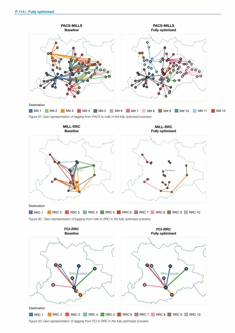
P 114 | Fully optimised
Figure 92 : Geo-representation of tagging from mills to RRC in the fully optimised scenario
Figure 91: Geo-representation of tagging from PACS to mills in the fully optimised scenario
PACS-MILLS
MILL-RRC
Fully optimised
Fully optimised
BaselinePACS-MILLS
BaselineMILL-RRC
Figure 93: Geo-representation of tagging from FCI to RRC in the fully optimised scenario
FCI-RRCFully optimisedBaseline
FCI-RRC
RRC 1 RRC 2 RRC 3 RRC 4 RRC 5 RRC 6 RRC 7 RRC 8 RRC 9 RRC 10
Destination
RRC 1 RRC 2 RRC 3 RRC 4 RRC 5 RRC 6 RRC 7 RRC 8 RRC 9 RRC 10
Destination
Mill 1 Mill 2 Mill 3 Mill 4 Mill 5 Mill 6 Mill 7 Mill 8 Mill 9 Mill 10 Mill 11 Mill 12
Destination

Optimisation of TPDS Supply Chain | P 115
Figure 94: Geo-representation of tagging from RRC to FPS (rice only) in the fully optimised scenario
13.5. CHANGES REQUIRED TO IMPLEMENT THE SCENARIOPOLICY CHANGE
• Classification of Supply Zones in the Food Security Rules and assigning of responsibilities.• Revision in the methodology for contracting of transporters including contracting terms, transportation rate
etc. to accommodate recommendation to move from per Qtl. rate to per Qtl. per Km. rate for the last leg i.e. RRC to FPS.
TECHNICAL CHANGE
• Changes to the SCMS and P-PAS databases on tagging of nodes: i.e. tagging of mills to RRCs and RRCs to FPS in SCMS and tagging of PACS to mills in the P-PAS system
• Changes to the SCMS and P-PAS Databases on allocation of nodes: i.e. allocation of mills in P-PAS and allocation of rice at each RRC from mills in SCMS.
OPERATIONAL CHANGE
• Contracting of new Transport agents (L1 and L2 transporters) or changes to existing contracts to accommodate changes in rates of transportation, allocation and tagging.
• Preparation of new allocation orders based on the changes in tagging of RRC to FPS.• Changes in the planning/execution, delivery schedules and pick up of paddy, rice and wheat between the
various nodes.
RRC-FPSFully optimisedBaseline
RRC-FPS
RRC 1 RRC 2 RRC 3 RRC 4 RRC 5 RRC 6 RRC 7 RRC 8 RRC 9 RRC 10
Origin

P 116 | Fully optimised

Optimisation of TPDS Supply Chain | P 117
ANNEXURES

P 118 | Annexures
Figure 1: Process for the proof of concept for optimisation of supply chain of TPDS, Dhenkanal ...................... 18Figure 2: Status of automation in the entire supply chain of Odisha ................................................................... 25Figure 3: Mapping of the supply chain for Dhenkenal.......................................................................................... 26Figure 4: Sample output map of PACS to Mills in baseline .................................................................................. 29Figure 5: Total distance and cost of transportation by leg for the baseline 5 ...................................................... 35Figure 6: Tagging and volume from PACS to mills in baseline ............................................................................. 36Figure 7: Distance and cost of transportation from PACS to Mill in baseline ...................................................... 36Figure 8: Volume and cost of transportation of paddy over distance range in baseline ...................................... 37Figure 9: Tagging and volume of rice and wheat from mills and FCI respectively to RRC in baseline ................ 37Figure 10: Distance and cost of transportation from mills to RRCs and FCI to RRC in baseline ........................ 38Figure 11: Total Distance from Mills to RRC in baseline ...................................................................................... 38Figure 12: Tagging and volume of rice and wheat from RRC to FPS in baseline ................................................. 38Figure 13: Distance and cost of transportation from RRC to FPS in baseline ..................................................... 39Figure 14: Geo-representation of tagging from PACS to Mill in baseline ............................................................. 39Figure 15: Geo-representation of tagging from Mill to RRC in baseline .............................................................. 40Figure 17: Geo-representation of tagging from RRC to FPS in baseline ............................................................. 40Figure 16: Geo-representation of tagging from FCI to RRC in baseline .............................................................. 40Figure 18: Total distance and cost of transportation by leg for the baseline with change in transport
contracting ......................................................................................................................................... 43Figure 19: Distance and cost of transportation for all legs in the optimising PACS tagging scenario ................. 47Figure 20: Tagging of PACS to Mill in the optimising PACS tagging scenario ..................................................... 48Figure 21: Volume of paddy from PACS to Mill in the optimising PACS tagging scenario .................................. 49Figure 22: Average Distance/Qtl and cost of transportation from PACS to mills in the optimising PACS
tagging scenario ................................................................................................................................. 49Figure 23: Geo-Representation of tagging in the optimise PACS tagging scenario ............................................ 50Figure 24: Changes in total cost and distance in all legs for the scenario optimise leg 1 and 2 ......................... 53Figure 25: Tagging and volume of paddy from PACS to mills in the optimising leg 1&2 scenario ....................... 54Figure 26: Distance and cost of transportation from PACS to mills in the optimising leg 1 and 2 scenario ........ 54Figure 27: Tagging of mills to RRCs in the optimising leg 1 and 2 scenario ........................................................ 55Figure 29: Distance and costs of transportation from mills to RRCs in the optimising leg 1 and 2 scenario ...... 56Figure 30: Geo-representation of tagging between PACS and mills in the optimising leg 1 and 2 scenario ....... 56Figure 31: Geo-representation of tagging between Mill and RRC in the optimising leg 1 and 2 scenario ......... 57Figure 32: Total distance and cost of transportation for all legs in the optimising FPS tagging scenario ........... 61Figure 33: Tagging of FPS to RRCs (Rice) in the optimising FPS tagging scenario ............................................. 62Figure 34: Volume of rice and wheat from RRC to FPS in each block in the optimise FPS tagging scenario ..... 62Figure 36: Cost of transportation from RRC to FPS in the scenario optimising FPS tagging .............................. 63Figure 35: Distance travelled by FPS in the leg: RRC to FPS in the optimising FPS tagging scenario ............... 63Figure 37: Analysis of savings over a range of transportation rates for the last leg ............................................ 64Figure 38: Geo-representation of tagging from RRC to FPS in the optimising FPS tagging scenario ................ 64
ANNEXURE 1: LIST OF FIGURES

Optimisation of TPDS Supply Chain | P 119
Figure 39: Total distance and costs of transportation by each leg for the closing mills scenario ........................ 69Figure 40: Changes in tagging and volume from PACS to mills in the closing mills scenario ............................. 70Figure 41: Distance and cost of transportation from PACS to Mills in the closing mills scenario ....................... 70Figure 42: Tagging of mills to RRC in the closing mills scenario .......................................................................... 71Figure 43: Changes in volume of rice from mills to RRC in the closing mills scenario ........................................ 71Figure 44: Changes in distance and cost of transportation from mills to RRC in the closing mills scenario ....... 72Figure 45: Geo-representation of tagging of PACS to Mill in the closing mills scenario ...................................... 72Figure 46: Geo-representation of tagging of Mill to RRC in the closing mills scenario ........................................ 73Figure 47: Total distance and costs of transportation for all legs in this scenario closing PACS ........................ 77Figure 48: Tagging and volume of paddy from PACS to mills in the closing PACS scenario ............................... 78Figure 49: Changes in tagging and volume of paddy by block in the closing PACS scenario ............................ 78Figure 50: Distance and cost of transportation from PACS to mills for the closing PACS scenario .................... 79Figure 51: Geo-representation of tagging of PACS to mills in the closing PACS scenario .................................. 79Figure 52: Total Cost of transportation and distance for all legs in the closing FPS scenario ............................ 83Figure 53: Changes in the tagging and volume from RRCs to FPSs in the scenario closing FPS ...................... 84Figure 54: Changes in volume of rice and wheat from RRC to FPS(block) in the closing FPS scenario ............. 84Figure 55: Average distance travelled and total cost of transportation in the closing FPS scenario
(Rice and Wheat) ............................................................................................................................... 85Figure 56: Geo-representation of tagging from RRC to FPS in the closing FPS scenario ................................... 85Figure 57: Total cost and average distance/Qtl in all legs for the fully optimised with capacity
constraint scenario ............................................................................................................................. 89Figure 58: Tagging and Volume from PACS to mills in the fully optimised with capacity constraint scenario ..... 90Figure 59: Changes in volume of paddy from PACS to mills (example) in the fully optimised with capacity
constrained scenario .......................................................................................................................... 90Figure 60: Average distance/Qtl. and cost of transportation from PACS to mills in the fully optimised with
capacity constrained scenario ........................................................................................................... 91Figure 61: Tagging and volume of rice from mills to RRC in the fully optimised with capacity
constrained scenario .......................................................................................................................... 91Figure 62: Changes in volume of rice from mills to RRC in the fully optimised with capacity
constrained scenario .......................................................................................................................... 92Figure 63: Average distance/Qtl. and costs from mills to RRC in the in fully optimised with capacity
constrained scenario .......................................................................................................................... 92Figure 64: Tagging of volume from RRC to FPS in the fully optimised with capacity constrained scenario ....... 93Figure 65: Changes in volume from RRC to FPS (block) in the fully optimised with capacity
constraint scenario ............................................................................................................................. 93Figure 66: Average distance/Qtl. and cost of transportation from RRC to FPS in the fully optimised with
capacity constrained scenario ........................................................................................................... 94Figure 67: Geo-representation of tagging of PACS to mills in the fully optimised with capacity
constrained scenario .......................................................................................................................... 94Figure 68: Geo-representation of tagging of mills to RRC in the fully optimised with capacity
constrained scenario .......................................................................................................................... 95Figure 69: Geo Representation of Tagging of RRC to FPS in the fully optimised with capacity
constrained scenario .......................................................................................................................... 95Figure 70: Total Distance and cost of transportation for all legs in fully optimised with capacity
constraints +15% scenario ................................................................................................................ 99

P 120 | Annexures
Figure 71: Tagging and volume of paddy from PACS to mills in the fully optimised with capacity constraint +15% scenario ................................................................................................................ 100
Figure 72: Cost of transportation and distance travelled from PACS to mills in the fully optimised with capacity constraint +15% scenario ................................................................................................................ 100
Figure 73: Tagging and allocation of rice from mills to RRCs in the fully optimised with capacity constraints +15% scenario .............................................................................................................. 101
Figure 74: Tagging and allocation of wheat from FCI to RRCs in the fully optimised with capacity constraints +15% scenario .............................................................................................................. 101
Figure 75: Cost of transportation and distance from mills to RRC in the fully optimised with capacity constraint +15% scenario ............................................................................................................... 102
Figure 76: Cost of transportation and distance from FCI to RRC in the fully optimised with capacity constraint +15% scenario ................................................................................................................ 102
Figure 77: Tagging and volume from RRCs to FPS in fully optimised with capacity constarint +15% scenario ................................................................................................................ 103
Figure 78: Cost of transportation and distance from RRC to FPS (Rice and Wheat) in the fully optimised with capacity constraint +15% scenario .................................................................................................. 103
Figure 79: Geo-representation of tagging from PACS to Mills in fully optimised with capacity constarints +15% scenario .............................................................................................................. 104
Figure 80: Geo-representation of tagging from Mills to RRC in the fully optimised with capacity constarint +15% scenario ................................................................................................................ 104
Figure 81: Geo-representation of tagging from RRC to FPS in the scenario fully optimised with capacity constarint +15% ............................................................................................................................... 105
Figure 82: Total cost of transportation and average distance/Qtl. in all legs for the fully optimised scenario ... 109Figure 83: Tagging and volume of paddy from PACS to mills in the fully optimised scenario ........................... 110Figure 84: Cost of transportation and average distance/Qtl for PACS to mills in the fully optimised scenario . 110Figure 85: Tagging and volume of rice from mills to RRC in the fully optimised scenario ................................. 111Figure 86: Volume of wheat from FCI to RRC .................................................................................................... 111Figure 87:Total distance and cost of transportation from mills to RRC for the fully optimised scenario ........... 112Figure 88: Total distance and cost of transportation from FCI to RRC for the fully optimised scenario ............ 112Figure 90: Cost of transportation and distance of RRC to FPS in the fully optimised scenario ........................ 113Figure 89: Tagging and volume of rice and wheat from RRC to FPS ................................................................. 113Figure 91: Geo-representation of tagging from PACS to mills in the fully optimised scenario .......................... 114Figure 92 : Geo-representation of tagging from mills to RRC in the fully optimised scenario ........................... 114Figure 93: Geo-representation of tagging from FCI to RRC in the fully optimised scenario ............................. 114Figure 94: Geo-representation of tagging from RRC to FPS (rice only) in the fully optimised scenario ............ 115

Optimisation of TPDS Supply Chain | P 121
Table 1: Summary of scenarios and results .................................................................................................... 21Table 2: Key features of the supply chain in Odisha ........................................................................................ 24Table 3: Input fields and their description ........................................................................................................ 27Table 4: Current cost of transportation ............................................................................................................ 27Table 5: Scenarios and their description.......................................................................................................... 28Table 6: Key output KPI’s and their description ............................................................................................... 29Table 7: Sample output -excel file PACS to Mills in baseline .......................................................................... 30Table 9: Calculation of estimated current transport rate per Qtl. per Km. ....................................................... 34Table 8: Key statistics for the baseline ............................................................................................................ 34Table 10: Summary statistics for the baseline ................................................................................................... 35Table 11: Key outputs for the baseline ............................................................................................................. 35Table 12: Key statistics for the scenario baseline with change in transport contracting ................................... 42Table 13: Key output KPI’s for baseline with change in transport contracting ................................................. 43Table 14: Key statistics for optimising PACS tagging scenario ......................................................................... 46Table 15: Key output KPI’s for optimising PACS tagging scenario .................................................................... 47Table 16: Summary statistics for scenario Optimising Leg 1&2 ........................................................................ 52Table 17: Key output KPI’s for optimising leg 1&2 scenario .............................................................................. 53Table 18: Summary statistics for scenario optimising FPS tagging .................................................................. 60Table 19: Key output KPI’s for optimising leg 1&2 scenario .............................................................................. 61Table 20: Summary statistics for the scenario closing mills .............................................................................. 68Table 21: Key output KPI’s for scenario closing mills (costs in Rs.) .................................................................. 69Table 22: Summary statistics for the scenario closing PACS ............................................................................ 76Table 23: Key output KPI’s for scenario closing PACS ...................................................................................... 77Table 24: Summary statistics for the scenario closing FPS ............................................................................... 82Table 25: Key output KPI’s for the scenario Closing FPS .................................................................................. 83Table 26: Summary statistics for fully optimised with capacity constraints scenario ........................................ 88Table 27: Key output KPI’s for scenario fully optimised with capacity constraints ........................................... 89Table 28: Summary statistics for the scenario fully optimised with capacity constraint +15% ......................... 98Table 29: Key output KPI’s for scenario fully optimised with capacity constraint +15% .................................. 99Table 30: Summary statistics for the fully optimised scenario......................................................................... 108
ANNEXURE 2: LIST OF TABLES

P 122 | Annexures

Optimisation of TPDS Supply Chain | P 123
P 124 | Annexures