Optimisation of simultaneous train formation and carsorting at marshalling yards∗

Sara Gestrelius1, Florian Dahms2 and Markus Bohlin1

1SICS Swedish ICT ABBox 1263, SE-164 29 Kista, Sweden,{firstname.lastname}@sics.se

2RWTH Aachen, Chair of Operations ResearchKackertstrasse 7, 52072 Aachen, Germany

dahms@or.rwth-aachen.de

AbstractEfficient and correct freight train marshalling is vital for high quality carload freight trans-portations. During marshalling, it is desirable that cars are sorted according to their individualdrop-off locations in the outbound freight trains. Furthermore, practical limitations suchas non-uniform and limited track lengths and the arrival and departure times of trains needto be considered. This paper presents a novel optimisation method for freight marshallingscheduling under these circumstances. The method is based on an integer programmingformulation that is solved using column generation and branch and price. The approachminimises the number of extra shunting operations that have to be performed, and is evaluatedon real-world data from the Hallsberg marshalling yard in Sweden.

KeywordsShunting, Marshalling, Classification, Optimisation, Blocking, Column Generation

1 Introduction

To maximise the capacity of a carload transportation system a hub and spoke network isoften operated. The hubs are marshalling yards, where incoming cars are sorted into newoutbound trains. Outbound trains have predetermined service routes, and cars are assignedto trains that pass through their destination. This implies that cars have to be decoupled atintermediate stops, and to facilitate drop-off it is desirable that all the cars that are to bedecoupled at a certain location are right at the end of the train when the train reaches thislocation. For this reason, cars should be sorted according to their drop-off location, into socalled blocks, during marshalling. Furthermore, practical limitations such as non-uniformand limited track lengths, and arrival and departure times of the inbound and outbound trains,need to be respected. This paper presents a novel method for freight classification planningunder these circumstances. It is an extension of the work in Bohlin et al. [5], where columngeneration is used to find the classification schedule that minimises the number of extra carpull-backs, but where any car order within the outbound trains is assumed to be acceptable.

∗This work was funded in part by the Swedish Transport Administration (Trafikverket) under grant TRV210/29758.

1

The yard used as a case study is the Hallsberg marshalling yard in Sweden. The Hallsbergyard is the largest marshalling yard in Scandinavia, and its advantageous location makes it animportant hub in the Swedish freight transportation network. Like many other marshallingyards, the Hallsberg yard consists of three sub-yards: an arrival yard, a classification yard(also called classification bowl) and a departure yard. Inbound trains arrive to the arrival yardwhere their cars are decoupled from the line engine and undergo various inspections. Theuncoupled cars of the inbound train are then pushed over a hump and roll to various tracksin the classification yard by means of gravity and a switching system. On the classificationyard, the cars are sorted into new outbound trains. When all cars of an outbound train havebeen rolled to a classification track in the correct order the outbound train can be coupledand then either depart from the classification track, or be pulled to the departure yard anddepart from there. In Hallsberg an operational demand is that each track in the classificationyard may only contain cars of a single outbound train. That is, there must be a bijectionbetween trains and tracks at any point in time. However, due to capacity limitations andsorting requirements it is generally impossible to roll all cars straight to the tracks that havebeen reserved for their outbound trains. Therefore, some of the tracks in the classificationyard are used as a buffer area where cars of different trains may be temporarily stored. Thesetracks are called mixing tracks. The tracks used for building trains are called train formationtracks. At given points in time, a pull-back operation is performed which allows any subsetof cars to be moved from the mixing tracks to the train formation tracks. During a pull-backthe cars of a mixing track are coupled, pulled back over the hump by an engine, and thenimmediately pushed over the hump to once again be distributed on the classification tracks.The later is called a roll-in operation. For a more detailed description of the operations inHallsberg we refer to [6].

Although sorting according to blocks is omitted in Bohlin et al.[5], it is generallyincluded in previous literature on classification planning. Research has been performed onclassification yard operations since the 1950s, and reviews of the area are given by Gatto et al.[13] and more recently Boysen et al. [8]. Four basic methods for classification planning areSorting by trains, Sorting by block, Triangular Sorting and Geometric Sorting, all of whichinclude blocking. However, these methods determine the number of tracks and classificationsteps by the number of outbound trains and their blocks, and do not take arriving car orderinto consideration. This makes them robust against disruptions in the incoming car order,but also leads to an excessive use of capacity or pull-backs. Gatto et al. [13] provides agood overview of the trade-offs between the different algorithms. Dahlhaus et al. [10, 11]introduce the train marshalling problem and presents a radix sort scheme that exploit the carorder in the arriving trains (called pre-sortedness), and show that this reduces the number ofsorting steps from logW (n) to logW (k), where W is the number of classification tracks, nthe number of arriving cars and k the number of batches. A batch is the maximal sequence ofcars that are in the correct relative order in the inbound trains. Jacob et al. [14] also developa methodology that takes pre-sortedness into consideration by representing the classificationschedule of each car by a binary encoding, and then using the intrinsic properties of thisrepresentation to generate an optimal schedule. Further, they use their representation toencode and analyse the previously mentioned basic sorting algorithms. Beygang et al. [4]provide a lower bound on the objective, and upper and lower bounds on competitiveness forthe online version of the problem as well as give an optimal deterministic online algorithm.

The encoding in Jacob et al. [14] is also used to develop an integer programming (IP)model for deriving optimal classification schedules in Maue and Nunkesser [15]. The IP

2

model incorporates real world constraints such as multiple humps and track capacity, and itcan be extended to take departure times into consideration. The authors model the LausanneTriage Shunting yard, and report that an optimal schedule was found within 3 minutes.Further, this schedule requires one less pull-back and one less track than the planning methodcurrently used in Lausanne. The Hallsberg marshalling yard in Sweden has also beenmodelled using first mixed integer programming (MIP) and later pure IP by Bohlin et al.[6, 7, 5]. The three articles present more and more efficient MIP and IP formulations, andin the latest paper [5], an optimal classification schedule for five days is found within 13minutes for all 30 real world test cases. All models presented by Bohlin et al. [6, 7, 5] takethe additional constraints imposed by a car booking system into consideration.

The main contribution of this paper is a new model for optimised marshalling planningthat respects operational constraints and allows for cars to be sorted into blocks in theoutbound trains. Cars are simultaneously sorted by block and train, and car bookings onspecific trains are respected, i.e. cars need not depart with the next train going to theirdestination, but the freight transportation company can define exactly which train they want acertain car to depart with. As the generated schedule minimises the number of car pull-backswhile allowing for blocked outbound trains, it contributes to both efficient shunting andefficient freight transportations.

The paper is structured as follows. In Section 2, the mixing problem with car sortingaccording to blocks is formally defined, and in Section 3 the branch-and-price based columngeneration approach from Bohlin et al. [5] is presented. We also show how to extend thisformulation to allow for sorting by blocks. Section 4 describes the experimental setup andresults, and includes an analysis of how sorting by blocks affects the execution time andsolution quality. Finally, Section 5 concludes the paper and outlines future research.

2 Problem Definition

We are given a set of classification tracks O, a set of periods P , a set of car units Q, anda set of outbound trains R. We denote by B(r) ⊆ B the blocks belonging to train r, andQ(b) ⊆ Q the set of car units that belong to block b. A car unit consists of cars that belongto the same block and arrive with the same inbound train. For each car unit q ∈ Q, we aregiven its arrival time t(q), i.e., the time when its inbound train is rolled to the classificationyard from the arrival yard, its length s(q), and its corresponding outbound train r(q) ∈ R.Further, each car unit q ∈ Q belongs to a block b(q) ∈ B. The blocks have a natural order inwhich they must appear in the outbound train based on their geographical location. However,within a block no special ordering of cars is necessary. We denote by Q(r) ⊆ Q the set ofcar units that belong to train r. Further, each train r ∈ R has a departure time t(r), i.e., thetime when it leaves the classification bowl. The length s(r) of a train r is the sum of thelengths of its cars, s(r) :=

∑q∈Q(r) s(q).

For each classification track o ∈ O we are given its length s(o). Thus, a train r can beformed on track o if and only if s(r) ≤ s(o). Let R(o) denote the set of trains that can beformed on track o. At any point in time, a classification track may only contain cars of oneoutbound train, and each train is formed on exactly one classification track. We say that atrain r is active for the time interval during which its corresponding classification track isused exclusively for the formation of r. Further, we call the block currently being built onthe classification track the active block.

We define the strict partial order≺ on the set of outbound trains R such that r ≺ r′ if and

3

only if train r ∈ R can be scheduled directly before train r′ ∈ R on the same track. Whetherr ≺ r′ holds or not depends on the departure times of trains r and r′ as well as on technicalsetup times (e.g., brake inspection) and other car movements in the marshalling yard. This isfurther explained in Section 2.1. Note that antisymmetry is ensured as no two trains may beformed on one track at the same time.

As stated previously, capacity limitations and sorting requirements normally make itimpossible for all cars to be rolled straight to their train formation tracks. Therefore, we arealso given a set of mixing tracks where cars of different outbound trains can be temporarilystored. To simplify our model, we treat these tracks as one concatenated track, called themixing track. This simplification is valid as long as enough time is added to pull back all carson all physical mixing tracks each time the cars on the concatenated mixing track is pulledback.

The mixing track has a given length smix. A car that is stored on the mixing track is saidto be mixed. All mixed cars are pulled back to the arrival yard at certain predetermined times,and are then immediately pushed over the hump again so that the cars can be re-distributedon the classification tracks. All cars belonging to currently active blocks will be rolled totheir train formation tracks, while the remaining cars are rolled back to the mixing track.We call this operation a pull-back followed by a roll-in. A pull-back operation defines thebeginning of a period p ∈ P , and all cars that are sent to the mixing track after the start timet(p) of period p must remain mixed at least until the start of the next period at time t(p+ 1).

As an objective function, we choose to minimise the number of car pull-backs. There areseveral reasons for our choice of objective function. For each period during which a car ismixed, it will be subjected to a pull-back and roll-in operation, which takes effort and time,and wears down switches and tracks. Note that since no car can leave the mixing track untilthe next pull-back is performed, the total length of the mixed cars within a period is at itsmaximum at the end of the period.

How many cars that need to be mixed in a period depends on which blocks are active,and how long these blocks have been active for. The start time of a block b ∈ B(r′), denotedi(b, r), can be deduced if the blocks of train r′, and the train r that precedes train r′ on theclassification track, are known (see Section 2.1).

Although the car-ordering within an inbound train is assumed to be unknown, the roll-inorder of trains, and therefore of car units from different trains, is know. This means that theorder of car units on the mixing track is known to some extent, and in some cases we candeduce that car units belonging to different blocks are in the correct order on the mixingtrack, and should therefore be rolled to the train formation track in the same pull-back toavoid mixing cars for longer than necessary.

Let qbe be block b’s final car unit to be mixed. This implies that qbe is the final car unit tobe rolled in before block b’s active period starts. Further, assume that block b is immediatelyfollowed by block b′ in a train. Then all cars of b′ that arrives after qbe but before i(b′, r) canbe moved to the train formation track in the same pull-back as qbe if this pull-back ends theactive period of block b. If the pull-back does not end block b’s active period more cars aregoing to be rolled to block b after the pull-back, and all cars belonging to block b′ must bemixed for at least another period. Let’s call the set of car units that fulfill these criteria Qm,i.e. Qm is the car units that can be rolled to their train formation track in the same pull-backas cars of the previous block. Note that the pull-back that moves a car q ∈ Q(b′) ∩Qm tothe train formation track will be the pull-back that starts off the active period of block b′,but that there may be other mixed cars q ∈ Q(b′)\Qm that have to be mixed for yet another

4

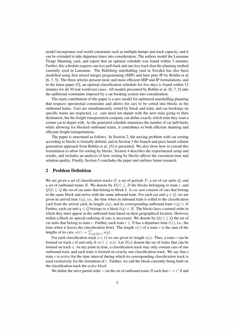
period as they were rolled in before t(qbe). An example of this is shown in Figure 1, wherecar q12 = q1e , and cars q22 , q

23 ∈ Qm and can be rolled to the train formation track in pull P1

while car q21 6∈ Qm and has to wait until pull P2.

r 1 2

t(q11) t(q21) t(q12) t(q22) t(q13) t(q23)P1

P2t(q24) t(q25)

q11

q21

q12

q23 ∈ Qm

q22 ∈ Qm

q21 6∈ Qm

t(r′)t(r)

Time

Train r′: Locomotive q13 q11q12q

22q

23 q24 q25q21

Figure 1: An example of cars of different blocks being in the correct order on the mixingtrack. Train r′ consists of two blocks and train r of one. The boxes represent the activeperiods of the trains and blocks, and the arrival times of the cars qbi ∈ r′ are plotted abovethe active period boxes. Car units are denoted qbi , where b is the block, and i an index toseparate the car units from each other. The departure times of the trains are shown by circlesunderneath the boxes. Pull-backs are represented by P , and the cars that are mixed when apull-back is executed are printed above the pull-back in the order that they were rolled to themixing track (so e.g. car q11 will be the first car to be rolled into the classification yard afterpull-back P1). Also, the final car ordering of train r′ is shown in the bottom of the picturewhere the cars have been plotted right underneath the times when they’re rolled to the trainformation track.

The number of extra car roll-ins needed if train r is followed by train r′ on a classificationtrack can now be calculated as follows:

c(r, r′) =∑

q∈Q(r′)

c(q, r)

wherec(q, r) = |q| · |P (q, r)|

is the number of extra roll-ins needed for car unit q if its train is shunted after r, and

P (q, r) =

∅ if i(b(q), r) ≤ t(q){p ∈ P : t(p) > t(q) ∧ t(p− 1) ≤ i(b(q), r)} elseif q 6∈ Qm

{p ∈ P : t(p) > t(q) ∧ t(p− 1) < i(b(q), r)} else

is the set of all periods in which q will be mixed, when its train is shunted after r. |q| is

5

defined as the number of cars in car unit q. Note that if p is the first pull-back in P , t(p− 1)is defined as the very first point in time.

Likewise, the length of cars that need mixing in each period, denoted sp(r, r′), is givenby,

sp(r, r′) =∑

b∈b(r′)

sp(b)

where,

sp(b) =

∑

q∈Q(b):t(q)<min(i(b,r),t(p+1))

s(q), if t(p) < i(b, r)∑q∈Q(b)\Qm:t(q)<min(i(b,r),t(p+1))

s(q), if t(p) = i(b, r)

0, otherwise.

The formulae above calculate the cost of train r′ if it’s scheduled straight after train r ona classification track. However, in a schedule there will also be a first train on each formationtrack. In Bohlin et al. [5] all cars belonging to the first train on a track will always be rolledstraight to this formation track. However, when sorting cars into blocks some of the carsof this first train may need to be mixed. To calculate the mixing cost of the first train animaginary train, u, with a departure time at 0.0, is introduced. The number of pull-backsincurred by the first train, c(u, r), can then be calculated using the formula above. Likewise,the mixing length, sp(u, r) can be calculated using the formula above and the same imaginarypredecessor train u.

Deducing active periods of blocksThe start time of a block b ∈ B(r′) where r′ is scheduled to follow r on a formation tracko is denoted i(b, r), and the end time t(b, r). Also, let a block b be denoted by its naturalorder in the outbound train, i.e. call the block that needs to be built first on the track 1, thenext one 2 etc. But from the first block, the start time of a block will always be the endtime of the previous block, i.e. i(b+ 1, r) = t(b, r). Note that all cars belonging to a blockmust be rolled to the track after the start time of the active period of the block. The onlyexception to this rule are cars in Qm, which may be rolled to the formation track in thepull-back that starts the active period of their block. The start time of the first block of a trainr will be the departure time of the train preceding r on the formation track. Further, the endtime of a block’s active period is the time when its final car is rolled to the train formationtrack. This may be as a result of an initial roll-in (arrival) or a mixing track pull-back and itsfollowing roll-in. If a block b requires mixing, its end time is max(pb, lb) where lb = t(qf )and qf ∈ Q(b) is the car with the latest roll-in time, and pb is the time of the earliest pull-backafter i(b, r), or, if all the cars of the two blocks are in the correct order on the mixing track(i.e. every mixed car belonging to block b exists in the setQm), pb is the time of the pull-backthat ends the active period of block b − 1. In the latter case the active period of block bmay be very short, and only consist of the time it takes for its cars to be rolled-in after thepull-back. Blocks that do not require mixing always end with a roll-in, namely t(qf ). Giventhese simple rules the start and end times of all the active periods of all blocks of train r′

following a train r on a formation track can be calculated as described in Algorithm 1. Notethat in the final iteration of the algorithm the end time of the final block will be calculatedand saved as the start time of a dummy block b = |B(r′)|+ 1.

6

Algorithm 1: Blocking(r, r′), calculates the start time for all blocks in a train r′ giventhat its immediate predecessor is train r.

input :Two trains r, r′

output :Start times i(b, r) for all blocks b ∈ b(r′)i(1, r)← t(r)foreach b ∈ b(r′) in natural block order do

eb ← minqi∈Q(b) t(qi)lb ← maxqi∈Q(b) t(qi)Mb ← {qi|qi ∈ Q(b) : t(qi) ≤ i(b, r)}if eb > i(b, r) then

pb ← 0else

if |Mb| = |Mb ∩Qm| and the active period of b starts with a pull-back thenpb ← i(b, r)

elsepb ← minpi∈P :i(b,r)<t(pi) t(pi)

endendi(b+ 1, r)← max(pb, lb)

end

2.1 Sequences and Feasible Solutions

We define feasible solutions to our problem in terms of sequences of trains, which can beallocated to individual tracks. A sequence g is a totally ordered subset of trains, includingthe dummy train u which defines the beginning of each sequence. Let us denote the fact thattwo trains r, r′ ∈ R appear consecutively in a sequence g by (r, r′) ∈ g. We call (r, r′) ∈ ga pairing. Note that in a pair (r, r′) train r occupies the formation track before train r′. Forexample, given a sequence g = 〈u, r1, r2, r3〉, it holds that (r1, r2) ∈ g and (r2, r3) ∈ g, butnote that (r1, r3) 6∈ g and (r2, r1) 6∈ g. A sequence which is ordered by ≺ is feasible. Let Gdenote the set of feasible sequences. For each sequence g ∈ G and period p ∈ P , let sp(g)be the total length of the mixed cars from g in p, i.e.,

sp(g) =∑

(r,r′)∈g

sp(r, r′) .

Further, let c(g) be the sum of all extra roll-ins for g:

c(g) =∑

(r,r′)∈g

c(r, r′) .

A schedule f : O → G is an injective mapping from tracks to feasible sequences. Afeasible sequence g can be scheduled on a track o if and only if all trains of the sequence fiton the track, i.e., g ⊆ R(o). Let us denote by G(o) the set of all feasible sequences that canbe scheduled on track o. A feasible solution to our problem can now be defined as a schedulef that

7

1. assigns a feasible sequence to each track,

∀o ∈ O : f(o) ∈ G(o) ,

2. such that each train occurs exactly once in a sequence,

∀r ∈ R : ∃o ∈ O : r ∈ f(o) ∧ ∀o′ ∈ O : o 6= o′ → r 6∈ f(o′) ,

3. and such that in each period, the capacity of the mixing track is respected,

∀p ∈ P :∑o∈O

sp(f(o)) ≤ smix .

Feasible SequencesFor two trains (r, r′), where r departs before r′, to be comparable by ≺ the active periodsof all blocks b ∈ B(r′) must fit within the active period of train r′. The departure time oftrain r determines when the active period of r′ may start. If the departure time of r is earlierthan the arrival time of the earliest car of the first block of train r′ the two trains are triviallycomparable, else they are only comparable if there are enough pull-backs for all blocks oftrain r′ to be built before its departure time. The end-time of the final block of train r′ can becalculated using Algorithm 1, and if the end-time of the final active block is earlier than, orat the same time as, the departure time of train r′ minus a given time for technical set-up, thetwo trains are comparable by ≺ and may be used in the same sequence. An example of twofeasible and one infeasible train pairings is shown in Figure 2.

r 1 2

t(q2)P1 P2

t(r′)t(r)

Time

t(q1)P3 t(q2)

P4

(r, r′) feasible

r 1 2

t(q2)

t(r′)t(r)

t(q1) t(q2)

(r, r′) infeasible

r 1 2

t(q1)

t(r′)t(r)

t(q1) t(q2)

(r, r′) feasible

P1 P2 P3 P4

P1 P2 P3 P4

Figure 2: An example of two feasible pairings and one infeasible. Train r is not blockedwhile train r′ has two blocks. The active periods of the trains are marked with white boxes,and the active periods of block 1 and 2 of train r′ are marked with grey boxes of differentdarkness. The departure times are shown as circles underneath the active period boxes, andthe technical set-up time as a black thick line. The roll-in times of cars belonging to trainr′ are shown above the boxes, and the arrows show when the cars are rolled to the trainformation track. The block of a car is indicated as a subscript. For the pairing to be feasibleall cars of train r′ must be rolled to the train formation track before the technical set-uppreceding its departure time t(r′).

8

3 The column generation model

In this section we introduce the column generation model from Bohlin et al. [5] and describethe necessary adaptations to allow for sorting the cars into blocks in the outbound trains. Theessence of column generation is to reduce the problem size of a linear programming problem(LP) by starting out with a few variables and solving this reduced problem to optimality. Ifthe solution satisfies all the constraints of the full dual problem the solution will be optimalalso for the full LP, but if some constraints are broken more variables need to be introduced.In the model we use, the variables to be included are generated using a method called pricing,where the variable that corresponds to the most violated constraint in the full dual is found.As the shunting problem is an integer programming problem (IP) rather than an LP, we workwith the LP relaxation of the IP, and then branching is used to find an IP solution. For a morethorough explanation of column generation, see Derosiers and Lubbecke [12].

In this paper we briefly outline the integer programming model and its dual. For furtherdetails on the model and the branching algorithm, we refer to Bohlin et al. [5].

3.1 The IP model and its dual

We use variables xgo to encode whether a sequence g is assigned to a track o or not. Further,variables yro are included to encode that train r is assigned to track o, as this variable isuseful during branching. This gives the IP,

min∑o∈O

g∈G(o)

c(g) · xgo (1)

s.t.∑o∈O

yro ≥ 1 r ∈ R (2)∑g∈G(o)r∈g

xgo ≥ yro r ∈ R, o ∈ O (3)

∑g∈G(o)

xgo ≤ 1 o ∈ O (4)

∑o∈O

g∈G(o)

sp(g) · xgo ≤ smix p ∈ P (5)

x, y ∈ {0, 1} (6)

(1) is the objective function, i.e. the number of car pull-backs, and to adapt the IPformulation for sorting by blocks the formula for c(g) from Section 2 should be used.Inequalities (2) and (3) ensure that every train is present in at least one sequence. Should atrain be present in more than one sequence in the final solution all but one instance of thetrain can be removed. Inequality (4) ensures that at most one sequence is assigned to eachtrack. In inequality (5) the formula for sp(g) from Section 2 should be used to make sure thatthe mixing track capacity is never exceeded. The dual of the problem is then the following,

9

max∑r∈R

αr +∑o∈O

γo + smix∑p∈P

δp (7)

s.t. αr ≤ βro r ∈ R, o ∈ O (8)∑r∈g

βro + γo +∑p∈P

sp(g) · δp ≤ c(g) o ∈ O, g ∈ G(o) (9)

α, β ≥ 0 γ, δ ≤ 0 (10)

3.2 Pricing

In the pricing step we want to find the variable that violates∑r∈g

βro +∑p∈P

sp(g) · δp − c(g) ≤ −γo

the most for each track o. That is the variables that maximise,

maxg∈G(o)

∑r∈g

βro +∑p∈P

sp(g) · δp − c(g) . (11)

To this aim we make use of a directed graph G = (V,E), where the nodes representtrains as well as the start and end of a sequence (special nodes u and v), V = R(o) ∪ {u, v}.The edge set E includes an edge (u, r) and (r, v) for every train r ∈ R(o), and an edge(r1, r2) if r1 ≺ r2. Any path from u to v in G corresponds to a feasible sequence g ∈ G(o).

Next, weights should be added to the edges. The weights represent how much cost acertain train pairing adds to Expression (11). As pointed out previously the first train in thesequence may incur a cost when sorting according to blocks. This potential cost is addedto the edge (u, r) for every train r ∈ R(o), where u is once again treated as a dummy trainwith departure time 0.0:

• w(u,r) = βro +∑

p∈P sp(u, r) · δp − c(u, r)

• w(r1,r2) = βr2o +∑

p∈P sp(r1, r2) · δp − c(r1, r2)

• w(r,v) = 0

Now, for every sequence g ∈ G(o) there is one equivalent path in G which has a totalweight equal to ∑

r∈g

βro +∑p∈P

sp(g) · δp − c(g) ,

where sp(g) and c(g) are defined as in Section 2 and allow for sorting according toblocks. This is the quantity that should be maximised, which is done by finding the longestpath in G from u to v. Bohlin et al. [5] points out that the partial ordering of trains makes Gcycle-free, and therefore the longest path can be calculated in O(|V |+ |E|) time (see [9]).As the train graph could be close to complete, the complexity in our case would be O(|R|2).

10

4 Experiments

Case studyThe Hallsberg classification yard, which is the main hub for car-load rail freight in Sweden,was used as a case study. To evaluate the approach, a historic data set obtained from theSwedish Transport Administration (Trafikverket) was used. The set included trains thatarrived to or departed from the Hallsberg yard between December 2010 and May 2011.Further, the physical constraints of Hallsberg marshalling yard were taken from [3].

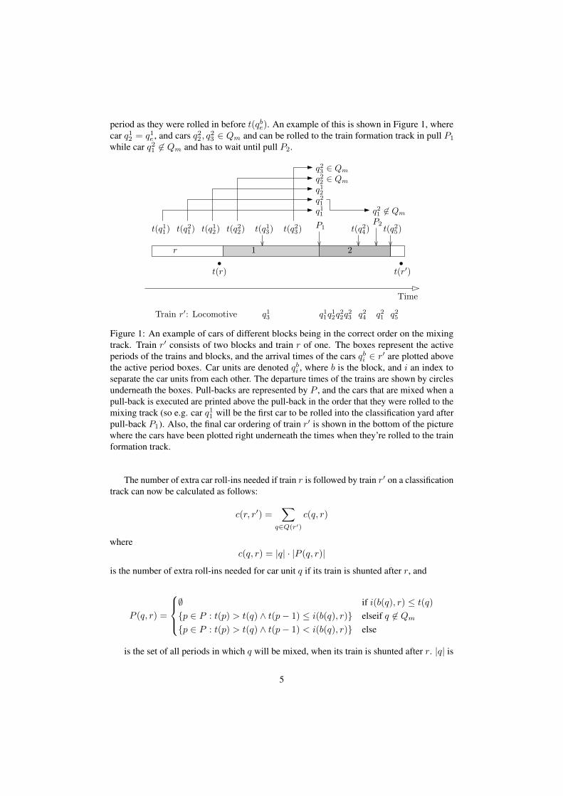
The geographical layout of the yard in Hallsberg can be seen in Figure 3. Hallsberg’sarrival yard consists of 8 tracks, while the classification yard has 32 tracks and the departureyard 23 tracks. The length of the arrival yard tracks range from 595 to 693 meters, and theclassification track lengths range from 374 to 760 meters. The departure yard tracks havelengths between 562 and 886 meters. Two classification tracks, of length 704 m and 724 m,were chosen as mixing tracks, giving a total mixing capacity of 1428 m.

Figure 3: Layout of the Hallsberg Marshalling yard, taken from [3]. The three sub-yards caneasily be identified, with the arrival yard to the left. But from the three sub-yards a numberof other tracks used for e.g. repair work are visible. These tracks were not included in theproblem set-up as they are normally not used for shunting. The image is not to scale.

Arrival and departure track scheduling was done in a pre-processing step as described inBohlin et al. [7]. Likewise, a hump schedule for roll-ins and pull-backs was generated usingthe same pre-processing code as in Bohlin et al. [7]. However, as sorting by blocks requiresmore shunting steps extra pull-backs were scheduled between two consecutive inbound trainroll-ins whenever possible. The time duration estimates used in the pre-processing, and whenadding extra pull-backs, were taken from [2].

The resulting data set consisted of 18 365 car groups. All cars in a car group arrive withthe same inbound train, and depart with the same outbound train. Note that this is differentfrom the car units used for generating a classification schedule that allows for sorting byblocks, as these car units consist of cars that arrive with the same inbound train, and belongto the same block in an outbound train. However, due to lack of better data car groups wereused as car units. Since operational planning normally is done for a few days at a time, theresulting data set was split into separate planning problems of three days each, resulting in atotal of 50 test cases. Every three day planning problem included all car groups that arrivedto or departed from the yard during the period.

Generating block dataUnfortunately real-life block data was not available for the sampling period. However, theHallsberg yard staff provided us with example data for one week to use as a basis for our

11

experimental setup. We used this example data to generate the block composition of trainsrandomly, based on the estimated frequency and composition of blocked trains in the exampledata set. Trains that require sorting by blocks normally depart at approximately the sametime each day, and a daily departure time pattern consisting of seven times was thereforechosen. This time pattern corresponded to times when blocked trains typically departed fromHallsberg. A sweep algorithm was then used to identify the first trains that departed after thetimes specified by the pattern and consisted of cars from more than one inbound train. Thelatter requirement is a consequence of the direct translation of car groups to car units, and theneed for at least two different car units to generate blocks. Trains that had been identified bythe sweep algorithm and that consisted of cars from only two inbound trains were assumedto have two blocks, all other trains that were identified were assumed to require two or threeblocks with equal probability. We restricted the number of blocks to at most three as theexample data set never contained more than three blocks for any train. The number of blocksthat a train required was sampled using the random module in Python 2.7 (for more detailson the random module see [1]).

After the blocked trains had been chosen, their cars had to be assigned to blocks. We calla blocked train that can be correctly built on one train formation track within its unrestrictedactive period, i.e. when its active period is determined by the roll-in times of the cars and thedeparture time of the train only, a feasible train. Whether a train is feasible or not dependson the blocks of the train, and the pull-back and roll-in schedule. Blocked trains that are notfeasible can never be built before their departure time and thereby render the entire probleminfeasible.

Let nrb = |B(r)| be the number of blocks of a train r, and let a block b be defined byits natural order, starting with 1. Then the following lemma states a sufficient condition forfeasible trains.

Lemma 1. A train r is feasible if for all cars q there exist at least nrb − b(q) pull-backsbefore t(r) but after t(q).

Although this condition is sufficient, it is not necessary. A trivial example of a feasibleblocked train that requires no pull-backs is a train whose cars are rolled in from the arrivalyard in the correct order. However, a feasible two block train that does not fulfill Lemma 1can be treated as a non-blocked train (as all cars of the train must already be in the correctorder during roll-in). Likewise, a feasible three block train not fulfilling Lemma 1 can betreated either as a train with no blocks (if all cars are rolled in in the correct order), or as atwo block train.

To sample a block for a car all blocks that were feasible for the car with respect toLemma 1 were identified. Then the random number generator of Python 2.7 was used tosample one of the feasible blocks and the car was assigned to this block. All feasible blockshad an equal probability of being chosen. To ensure that all blocks were represented at leastonce, the set of feasible cars was identified for each block, and then one car was sampledfrom each set and assigned to the respective block. This was done in the beginning of theblock-sampling, and the cars were sampled in the natural order of the blocks. Cars wereremoved from the sampling as soon as they had been assigned to a block. If a train did nothave any feasible cars for a certain block it was either assumed to not require sorting byblocks, or it was assumed to be a train of fewer blocks than originally sampled. More precise,two block trains were always assumed to not require sorting by blocks, while three blocktrains were re- marked as a two block trains and the block sampling was restarted.

12

The initial sweep algorithm identified 1054 trains to be blocked in the historic data. Outof these, 581 two block trains and 473 three block trains were sampled. However, due to lackof pull-backs 29 two block trains and 38 three block trains were rejected by the algorithm atlater stages. Further, 15 three block trains were re-marked as two block trains. Therefore thefinal experimental data included 567 two block trains and 420 three block trains. Out of the567 two block trains 260 were trivial, i.e. the blocks happened to be sampled such that allcars were rolled in from the arrival yard in the correct order. Likewise, 109 of the three blocktrains were trivial.

Introducing blocked outbound trains will decrease the number of feasible pairings as thenumber of pull-backs needed in the active period of a train is increased (see Section 2.1). Inour case, the number of feasible pairings was reduced from 135 514 to 131 755 for the entiresample period.

Technical detailsSCIP 3.1.0 was used as the branch-and-price framework, with CPLEX 12.5.00 as the LPsolver. The pre-processing code was run using Python 2.7.2. Experiments were performedon Linux workstations running openSUSE 12.1 with eight Intel Core i7-2600 quad-coreCPUs running at 3.4 GHz and equipped with 16 GB of RAM.

4.1 Results

Two different test cases, one with blocked outbound trains (called B-IP) and one without(N-IP), were executed and the results are presented in Table 1. Two different measurementsof car pull-backs are presented: P-EP is the number of extra car pull-backs that the problemset-up includes, while O-EP is the number of extra car pull-backs that would be needed toproperly sort all cars according to the generated classification schedule in an operationalsetting. The difference between the two measurements is largely caused by the pull-backsthat were added between consecutive train roll-ins. These pull-backs were scheduled withoutconsideration of how useful they would be, and therefore they are likely to not move anycars from the mixing track to the train formation tracks, but rather all mixed cars will just bepulled out to the arrival yard and then immediately rolled back to the mixing track. This isobviously an unnecessary operation, and in a real world setting the pull-back would not beexecuted. O-EP include only the extra pull-backs which are strictly necessary, while P-EPincludes all extra pull-backs present in the schedule. Further, while all pull-backs of N-IPmay be considered as “extra” pull-backs enforced by capacity limitations, a certain amountof pull-backs will be necessary for sorting the cars into blocks in B-IP. Therefore the totalnumber of pullbacks, as calculated by the formula in Section 3, is presented in brackets forB-IP. The extra pull-backs have been calculated as the total number of pull-backs minusthe number of pull-backs necessary for sorting the cars into blocks given that all the trains’active periods are unrestricted.

As can be seen in Table 1, the optimal solution is found for all test instances. Further, theaverage execution times for the two test cases are comparable, indicating that generating aschedule that allows for blocked outbound trains will not negatively affect the execution time.As expected the total number of pull-backs is greatly increased when blocking is introduced.However, the number of “extra” pull-backs enforced solely by capacity constraints remainslow. In fact, the average of P-EP enforced solely by capacity constraints is reduced whensorting cars according to blocks. This is explained by the fact that some of the pull-backs that

13

are necessary for sorting the cars into blocks will also alleviate capacity problems. However,the average O-EP is slightly higher for B-IP than for N-IP. This may be explained by thefact that more pull-backs will be useful when sorting cars into blocks. A car that spends thesame amount of time on a mixing track in B-IP and N-IP is therefore likely to be subjectedto more pull-backs in an operational setting if the mixing track is used not only for capacityalleviation but also for sorting cars according to blocks. The effect of this is not seen in P-EPas all pull-backs are included whether they are useful or not.

Table 1: The experimental results for two different test cases, one with blocked outboundtrains (B-IP) and one without (N-IP). P-EP are the number of extra pull-backs as definedby the problem set-up, while O-EP are the extra pull-backs that need to be carried out inan operational setting to sort the cars according to the generated classification schedule.The execution times and optimality gaps are also included. x is the arithmetic mean. Theexecution time is reported as clock-seconds, and includes problem set-up and post-processing.

Instance N-IP B-IPTrains Groups P-EP O-EP Time Gap P-EP (Tot) O-EP (Tot) Time Gap

(#) (#) (#) (#) (s) (%) (#) (#) (#) (#)1 65 257 0 0 10.2 0 0 (82) 0 (44) 8.5 02 107 581 68 33 124.5 0 48 (474) 34 (306) 99.9 03 35 148 0 0 1 0 0 (162) 0 (76) 1.2 04 88 340 0 0 29.9 0 0 (248) 0 (106) 44.8 05 14 46 0 0 0.1 0 7 (9) 7 (8) 0.1 06 55 170 0 0 3.3 0 0 (267) 0 (133) 3.3 07 44 170 0 0 2.6 0 0 (109) 0 (31) 2.8 08 51 155 0 0 3.8 0 0 (49) 0 (39) 2.8 09 70 268 0 0 12 0 0 (89) 0 (31) 11.3 010 44 155 0 0 2.2 0 0 (23) 0 (12) 2.6 011 113 575 89 38 191.2 0 61 (500) 53 (335) 154.8 012 57 282 0 0 4.4 0 0 (262) 0 (194) 4.7 013 91 485 30 28 43.4 0 17 (278) 17 (224) 38.7 014 80 440 4 2 25.4 0 0 (276) 0 (216) 24.8 015 63 259 0 0 7.6 0 0 (118) 0 (52) 6.5 016 73 308 0 0 9 0 0 (162) 0 (84) 8.1 017 53 229 0 0 4.6 0 0 (64) 0 (33) 3.6 018 97 485 5 3 51.8 0 3 (144) 2 (69) 61.7 019 66 296 0 0 5.5 0 0 (449) 0 (258) 5.1 020 78 440 18 16 15.7 0 9 (177) 8 (104) 14.6 021 75 371 0 0 12.3 0 0 (600) 0 (370) 13.9 022 59 251 0 0 8.8 0 0 (413) 0 (260) 8.3 023 106 594 64 54 70.3 0 51 (651) 51 (420) 52.4 024 43 200 0 0 1.5 0 0 (561) 0 (352) 1.7 025 108 538 3 3 93.5 0 0 (455) 0 (277) 66.8 026 74 327 0 0 10.9 0 0 (269) 0 (132) 9.2 027 82 467 4 2 14.2 0 2 (208) 2 (158) 14.1 028 72 413 130 24 12.1 0 130 (222) 68 (140) 5.6 029 62 259 0 0 8.1 0 0 (286) 0 (156) 7.2 0

14

Table 1: The experimental results (continuation from previous page).

Instance N-IP B-IPTrains Groups P-EP O-EP Time Gap P-EP (Tot) O-EP (Tot) Time Gap

(#) (#) (#) (#) (s) (%) (#) (#) (#) (#)30 103 572 29 20 173.5 0 21 (352) 21 (246) 169.6 031 50 234 0 0 3.1 0 0 (267) 0 (189) 3.1 032 118 715 100 81 130.4 0 64 (599) 59 (481) 156 033 78 420 1 1 13.1 0 0 (392) 0 (212) 16.1 034 88 492 49 39 36.3 0 20 (236) 16 (187) 43.7 035 84 503 14 9 36 0 3 (471) 3 (310) 28.6 036 65 288 0 0 6.8 0 0 (204) 0 (71) 7 037 94 546 118 78 49.4 0 85 (682) 63 (456) 41.8 038 51 268 0 0 4.5 0 0 (345) 0 (253) 5.6 039 111 640 86 76 151.4 0 67 (483) 67 (355) 148 040 59 269 0 0 5.1 0 0 (411) 0 (269) 4.8 041 95 513 158 62 47 0 145 (261) 83 (150) 54.7 042 86 514 29 22 21.3 0 28 (364) 25 (310) 29.4 043 70 319 6 4 9.9 0 6 (245) 5 (106) 14.6 044 84 503 14 12 37.8 0 7 (464) 6 (298) 32.4 045 5 9 0 0 0 0 0 (0) 0 (0) 0 046 91 470 19 12 24 0 4 (503) 4 (444) 33.2 047 71 391 0 0 6.8 0 0 (273) 0 (177) 5.3 048 94 533 247 118 45.2 0 235 (373) 187 (294) 62.5 049 74 413 4 4 13.3 0 3 (231) 3 (149) 20.2 050 56 244 0 0 4.4 0 0 (148) 0 (107) 4.6 0x 73.0 367.3 25.8 14.8 32.0 0 20.3 (298.2) 15.7 (193.7) 31.2 0

5 Conclusions

In this paper we introduced a novel approach for optimisation of simultaneous car sorting andtrain formation for freight shunting yards. The approach builds on the integer programmingapproach of Bohlin et al. [5] to enable the generation of classification schedules that allowfor cars to be sorted into blocks within outbound trains. This is accomplished by constructingnew formulae for calculating the mixing and pull-back costs, as well as adapting the pricingalgorithm. Experiments were performed on real traffic data from Hallsberg marshalling yard,generated block data, and a planning horizon of three days. The new model found an optimalsolution within three minutes for all 50 test instances, and the results show that althoughthe solutions require more car pull-backs in total, the number of extra pull-backs enforcedby capacity constraints is comparable with the number of extra pull-backs that is requiredwhen no outbound trains have blocks. In fact, if all pull-backs that were included in theproblem set-up are executed, the number of extra pull-backs enforced solely by capacityconstraints is reduced slightly when sorting the cars into blocks. This is because some ofthe pull-backs that are necessary for sorting (and hence not extra) also alleviate the capacityproblem. However, if only the useful pull-backs are executed, the number of extra pull-backs

15

is slightly increased when including sorting by blocks. This is explained by the fact that morepull-backs are useful in the blocked problem, and therefore a car that has been mixed forcapacity reasons is likely to be subjected to more pull-backs while waiting for track capacityto become available.

5.1 Future Work

There is a number of ways in which this method could be further improved. First of all,the heuristic used to decide the roll-in and pull-back times does not take blocking intoconsideration. Changing the heuristic such that blocking is included would most likelyimprove our results. Further, in this paper the mixing track modelling is simplified, and weview the different mixing tracks as one long track. In reality there are many mixing tracks,and they could be pulled-out at different times providing an opportunity to sort cars by blockson the mixing tracks, and thereby make better use of the yard capacity. For this reason, moredetailed mixing-track modelling is highly desirable. For the methods described in this paperto be applicable in real operations, robustness and efficient ways to update the schedule andextend the planning horizon are also important topics to address.

Acknowledgments

We are grateful to Stefan Huss and Pelle Andersson at Green Cargo AB for providinginformation and data on the shunting process in Hallsberg, and to the staff at the Hallsbergshunting yard for providing example data and for helpful and interesting discussions. Finally,we would like to thank Hans Dahlberg at the Swedish Transport Administration for hissupport.

References

[1] Python v2.7.3 documentation chapter 9.6. random –generate pseudo-random numbers.http://docs.python.org/2/library/random.html, Jan. 2013.

[2] C. Alzen. Handbok BROH 313.00700: Trafikeringsplan Hallsbergs rangerbangard.Banverket, May 2006.

[3] K.-A. Averstad. Handbok BROH 313.00001: Anlaggningsbeskrivning Hallsbergsrangerbangard. Banverket, February 2006.

[4] K. Beygang, S. O. Krumke, and F. Dahms. Train marshalling problem - algorithms andbounds -. Technical Report 132, TU Kaiserslautern, Fachbereich Mathematik, 2010.

[5] M. Bohlin, F. Dahms, H. Flier, and S. Gestrelius. Optimal Freight Train Classificationusing Column Generation. In D. Delling and L. Liberti, editors, 12th Workshop onAlgorithmic Approaches for Transportation Modelling, Optimization, and Systems,volume 25 of OpenAccess Series in Informatics (OASIcs), pages 10–22, Dagstuhl,Germany, 2012. Schloss Dagstuhl–Leibniz-Zentrum fuer Informatik.

[6] M. Bohlin, H. Flier, J. Maue, and M. Mihalak. Hump Yard Track Allocation with Tem-porary Car Storage. In The 4th International Seminar on Railway Operations Modelling

16

and Analysis (RailRome), 2011. Available on http://soda.swedish-ict.se/5089/.

[7] M. Bohlin, H. Flier, J. Maue, and M. Mihalak. Track Allocation in Freight-TrainClassification with Mixed Tracks. In 11th Workshop on Algorithmic Approaches forTransportation Modelling, Optimization, and Systems, volume 20 of OpenAccess Seriesin Informatics (OASIcs), pages 38–51, Dagstuhl, Germany, 2011. Schloss Dagstuhl–Leibniz-Zentrum fur Informatik.

[8] N. Boysen, M. Fliedner, F. Jaehn, and E. Pesch. Shunting yard operations: Theoreticalaspects and applications. European Journal of Operational Research, 220(1):1 – 14,2012.

[9] T. Cormen, C. Leiserson, R. Rivest, and C. Stein. Introduction To Algorithms. MITPress, 3rd edition, 2009.

[10] E. Dahlhaus, P. Horak, M. Miller, and J. F. Ryan. The train marshalling problem.Discrete Applied Mathematics, 103(1–3):41–54, 2000.

[11] E. Dahlhaus, F. Manne, M. Miller, and J. Ryan. Algorithms for combinatorial problemsrelated to train marshalling. In Proceedings of the Eleventh Australasian Workshop onCombinatorial Algorithms (AWOCA), pages 7–16, 2000.

[12] J. Desrosiers and M. Lubbecke. A primer in column generation. In G. Desaulniers,J. Desrosiers, and M. Solomon, editors, Column Generation, pages 1–32. Springer,Berlin, 2005.

[13] M. Gatto, J. Maue, M. Mihalak, and P. Widmayer. Shunting for dummies: An introduc-tory algorithmic survey. In Robust and Online Large-Scale Optimization, volume 5868of LNCS, pages 310–337. Springer, 2009.

[14] R. Jacob, P. Marton, J. Maue, and M. Nunkesser. Multistage methods for freight trainclassification. Networks, 57(1):87–105, 2011.

[15] J. Maue and M. Nunkesser. Evaluation of computational methods for freight trainclassification schedules. Technical report, ARRIVAL Project, 2009.

17