Embed Size (px)
Citation preview
Faculdade de Engenharia da Universidade do Porto
Optimisation of an Evaporation Unit for a SOFC APU
Samuel Gouveia Da Cunha
Master in Electrical and Computer Engineering
Supervisor: Adriano Da Silva Carvalho (PhD) Co-Supervisor: Michael Reißig (Dipl.-Ing.)
April 2014

© Samuel Gouveia da Cunha, 2014

i
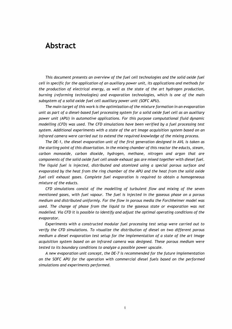
Abstract
This document presents an overview of the fuel cell technologies and the solid oxide fuel
cell in specific for the application of an auxiliary power unit, its applications and methods for
the production of electrical energy, as well as the state of the art hydrogen production,
burning (reforming technologies) and evaporation technologies, which is one of the main
subsystem of a solid oxide fuel cell auxiliary power unit (SOFC APU).
The main target of this work is the optimization of the mixture formation in an evaporation
unit as part of a diesel-based fuel processing system for a solid oxide fuel cell as an auxiliary
power unit (APU) in automotive applications. For this purpose computational fluid dynamic
modelling (CFD) was used. The CFD simulations have been verified by a fuel processing test
system. Additional experiments with a state of the art image acquisition system based on an
infrared camera were carried out to extend the required knowledge of the mixing process.
The DE-1, the diesel evaporation unit of the first generation designed in AVL is taken as
the starting point of this dissertation. In the mixing chamber of this reactor the educts, steam,
carbon monoxide, carbon dioxide, hydrogen, methane, nitrogen and argon that are
components of the solid oxide fuel cell anode exhaust gas are mixed together with diesel fuel.
The liquid fuel is injected, distributed and atomized using a special porous surface and
evaporated by the heat from the ring chamber of the APU and the heat from the solid oxide
fuel cell exhaust gases. Complete fuel evaporation is required to obtain a homogeneous
mixture of the educts.
CFD simulations consist of the modelling of turbulent flow and mixing of the seven
mentioned gases, with fuel vapour. The fuel is injected in the gaseous phase on a porous
medium and distributed uniformly. For the flow in porous media the Forchheimer model was
used. The change of phase from the liquid to the gaseous state or evaporation was not
modelled. Via CFD it is possible to identify and adjust the optimal operating conditions of the
evaporator.
Experiments with a constructed modular fuel processing test setup were carried out to
verify the CFD simulations. To visualize the distribution of diesel on two different porous
medium a diesel evaporation test setup for the implementation of a state of the art image
acquisition system based on an infrared camera was designed. These porous medium were
tested to its boundary conditions to analyze a possible power upscale.
A new evaporation unit concept, the DE-7 is recommended for the future implementation
on the SOFC APU for the operation with commercial diesel fuels based on the performed
simulations and experiments performed.

ii
iii
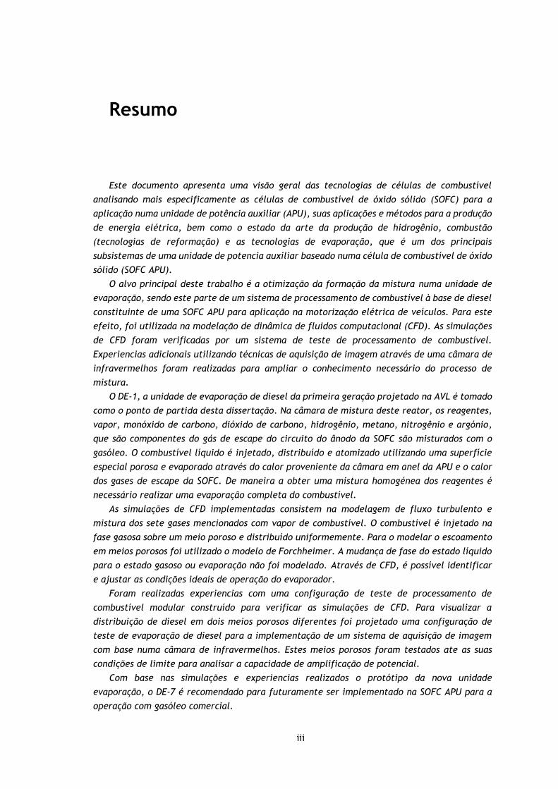
Resumo
Este documento apresenta uma visão geral das tecnologias de células de combustível
analisando mais especificamente as células de combustível de óxido sólido (SOFC) para a
aplicação numa unidade de potência auxiliar (APU), suas aplicações e métodos para a produção
de energia elétrica, bem como o estado da arte da produção de hidrogênio, combustão
(tecnologias de reformação) e as tecnologias de evaporação, que é um dos principais
subsistemas de uma unidade de potencia auxiliar baseado numa célula de combustível de óxido
sólido (SOFC APU).
O alvo principal deste trabalho é a otimização da formação da mistura numa unidade de
evaporação, sendo este parte de um sistema de processamento de combustível à base de diesel
constituinte de uma SOFC APU para aplicação na motorização elétrica de veículos. Para este
efeito, foi utilizada na modelação de dinâmica de fluidos computacional (CFD). As simulações
de CFD foram verificadas por um sistema de teste de processamento de combustível.
Experiencias adicionais utilizando técnicas de aquisição de imagem através de uma câmara de
infravermelhos foram realizadas para ampliar o conhecimento necessário do processo de
mistura.
O DE-1, a unidade de evaporação de diesel da primeira geração projetado na AVL é tomado
como o ponto de partida desta dissertação. Na câmara de mistura deste reator, os reagentes,
vapor, monóxido de carbono, dióxido de carbono, hidrogênio, metano, nitrogênio e argónio,
que são componentes do gás de escape do circuito do ânodo da SOFC são misturados com o
gasóleo. O combustível líquido é injetado, distribuído e atomizado utilizando uma superfície
especial porosa e evaporado através do calor proveniente da câmara em anel da APU e o calor
dos gases de escape da SOFC. De maneira a obter uma mistura homogénea dos reagentes é
necessário realizar uma evaporação completa do combustível.
As simulações de CFD implementadas consistem na modelagem de fluxo turbulento e
mistura dos sete gases mencionados com vapor de combustível. O combustível é injetado na
fase gasosa sobre um meio poroso e distribuído uniformemente. Para o modelar o escoamento
em meios porosos foi utilizado o modelo de Forchheimer. A mudança de fase do estado líquido
para o estado gasoso ou evaporação não foi modelado. Através de CFD, é possível identificar
e ajustar as condições ideais de operação do evaporador.
Foram realizadas experiencias com uma configuração de teste de processamento de
combustível modular construído para verificar as simulações de CFD. Para visualizar a
distribuição de diesel em dois meios porosos diferentes foi projetado uma configuração de
teste de evaporação de diesel para a implementação de um sistema de aquisição de imagem
com base numa câmara de infravermelhos. Estes meios porosos foram testados ate as suas
condições de limite para analisar a capacidade de amplificação de potencial.
Com base nas simulações e experiencias realizados o protótipo da nova unidade
evaporação, o DE-7 é recomendado para futuramente ser implementado na SOFC APU para a
operação com gasóleo comercial.

iv

v
Acknowledgements
The present dissertation was done during my work at the Fuel Cell Department of AVL List
GmbH in Graz.
First and foremost, I would like to express my deepest gratitude to my supervisor Michael
Reißig who allowed me to work on this dissertation and for all his knowledge, kindness, patience
encouragement and continual help. He was always ready for a meeting with me to discuss the
latest developments, problems and ideas of the work. I thank him for his constant commitment
and interest with all my heart.
My sincere thanks goes also to my numerous studies, diploma and working colleagues in the
fuel cell and aftertreatment systems department. The successful implementation of this work
would not have been possible without their help. To Juergen Rechberger for letting me be a
part of such a great and passionate team, full of potential, devoted with heart and soul, working
always with great effort and high performance and a great willingness and desire to push the
boundaries and go always further. To my dear colleagues Simone Lion, Fabian Rasinger, Roger
Cascante, Mathias Spilmann, Konrad Konlechner, René Voetter, Michael Seidl Jörg Mathé,
Martin Hauth, Doris Schoenwetter, Richard Schauperl, Katharina Renner, Michael Pfragner,
Johannes Lackner, Stefan Planitzer and Vincent Lawlor for the exchange of ideas and the
pleasant and comfortable working atmosphere. Horst Kiegerl, Markus Schaffhauser, Markus
Kuerzl, Mario Koroschetz and Dominik Juritsch, for their technical knowledge, experience and
help. Markus Thaler for the support in optical measurement systems and constructive
discussions. Roman Lucrezi that helped me with his genius and experience in physics and fluid-
dynamic modelling. Christopher Sallai for his genius in the support about CAD design. Thank
you all from the bottom of my heart.
I’m also grateful to my professor and supervisor Prof. Dr. Adriano da Silva Carvalho for the
knowledge, encouragement, life experience and advices that he transmitted me throughout my
academic career.
I also thank my friends from FEUP especially, Eduardo Mota, Sandro Vale, Alexandre Roças,
Duarte Sousa, Francisco Cunha, José Autilio, Antonio Patricio, Pedro Pinto, Patricio Lima and
Pedro Alves for their friendship, encouragement and support along my academic career.
I thank my friend Tuan Nguyen for his lifelong friendship, for encouraging me constantly
and giving me always important advices. He has always been like a brother to me.
My special thanks goes also to my parents and my brother, who helped and supported me
during the entire time, without them none of this would be possible.
Finally, I thank for the help and blessing of God, without which no success is possible.

vi

vii
“Strength does not come from winning. Your struggles develop your strengths. When you go
through hardships and decide not to surrender, that is strength.”
Arnold Schwarzenegger

viii
ix
Índex
Abstract ............................................................................................ i
Resumo ...........................................................................................iii
Acknowledgements ..............................................................................v
Índex .............................................................................................. ix
List of figures .................................................................................... xi
List of tables ................................................................................... xxi
Abbreviations and Symbols ................................................................ xxiii
Chapter 1 ......................................................................................... 1
Introduction ..................................................................................................... 1
1.1. Motivation ............................................................................................... 3
1.2. Goals of the dissertation .............................................................................. 5
1.3. Document Outline ...................................................................................... 5
1.4. Methodology ............................................................................................. 6
1.4.1. Hardware ........................................................................................... 6 1.4.2. Software ............................................................................................ 7
Chapter 2 ........................................................................................ 11
State of the Art .............................................................................................. 11
2.1. Fuel Cell ............................................................................................... 11
2.1.1. Evolution ......................................................................................... 11 2.1.2. Operation standard procedures .............................................................. 11 2.1.3. Thermodynamics and efficiency.............................................................. 12 2.1.4. Fuel Cell Types .................................................................................. 14 2.1.5. The Solid Oxide Fuel Cell ...................................................................... 14
2.2. Basic principles of fuel gas production from hydrocarbons ................................... 16
2.2.1. Basic concepts ................................................................................... 17 2.2.2. Reforming methods ............................................................................. 17 2.2.3. Soot formation and carbon deposit .......................................................... 23 2.2.4. Reformers for Fuel Cells ....................................................................... 25
2.3. Evaporation on flat surfaces........................................................................ 27
2.3.1. Definition of the characteristic boiling modes ............................................ 27 2.3.2. Evaporation on porous surfaces .............................................................. 33
x
2.4. Concept of a Fuel Cell APU System based on liquid fuels ..................................... 39
2.4.1. AVL SOFC APU System .......................................................................... 40
Chapter 3 ........................................................................................ 49
Simulations, redesign and optimization of the evaporator ........................................... 49
3.1. Physical parameters ................................................................................. 49
3.2. System requirements ................................................................................ 50
3.3. Evaporator experimental fuel processing simulation .......................................... 51
3.4. Dynamic flow modelling (CFD) ..................................................................... 54
3.4.1. Pre-processing ................................................................................... 55 3.4.2. Solving ............................................................................................ 65 3.4.3. Post-processing .................................................................................. 72
Chapter 4 ........................................................................................ 93
Experimental Setup ......................................................................................... 93
4.1. Test Bench Setup ..................................................................................... 93
4.2. Testing Equipment ................................................................................... 94
4.2.1. Fuel Processing Test System .................................................................. 94 4.2.2. Test System for the Diesel Evaporation on Porous Surface ............................ 100
Chapter 5 ...................................................................................... 105
Practical Implementation and Evaluation .............................................................. 105
5.1. Commissioning of the Fuel processing Test System ........................................... 105
5.1.1. Heat up Procedures ........................................................................... 106 5.1.2. Operational Procedures ....................................................................... 106 5.1.3. Test Results ..................................................................................... 107
5.2. Commissioning of the Diesel Evaporation on Porous Surface Test System ................ 109
5.2.1. Heat up Procedures ........................................................................... 111 5.2.2. Image Acquisition and Test Execution ..................................................... 112 5.2.3. Image Processing and Results ................................................................ 114
Chapter 6 ...................................................................................... 123
Conclusion.................................................................................................... 123
6.1. Conclusion and Future Work ...................................................................... 123
Appendix A .................................................................................... 127
Miscellaneous Equations, Tables and Figures .......................................................... 127
Bibliography ................................................................................................. 143

xi
List of figures
Figure 1.1 Concept sketch of the SOFC APU [10] ........................................................ 4
Figure 1.2 Gas treatment process for a fuel cell system based on liquid fuels. GM=Gas mixture formation; SR=Steam reforming; ATR=Autothermal reforming; POX=Partial oxidation; Shift=CO-conversion; PROX=Selective CO-oxidation; PSA=Pressure Swing Adsorption; Membrane=membrane process; Methane=Methanisation ......................... 4
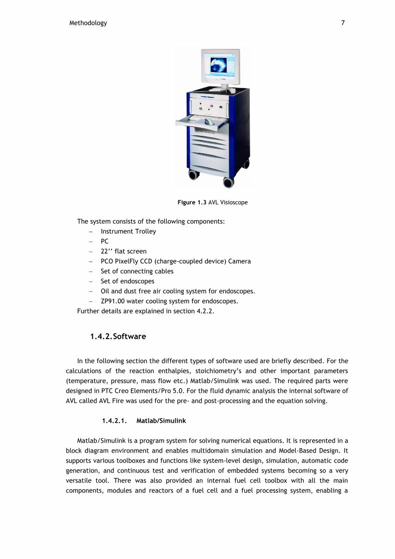
Figure 1.3 AVL Visioscope ................................................................................... 7
Figure 2.1 Principle of a fuel cell [17] .................................................................. 12
Figure 2.2 Functional diagram of the SOFC ............................................................ 14
Figure 2.3 Equilibrium composition and adiabatic temperature for partial oxidation of diesel fuel υeducts=25 ºC, p=1 bar, φ=0,65 [43] ................................................... 23
Figure 2.4 Temperature dependence of the product composition and soot formation in the heated steam reforming of Diesel fuel [43] ...................................................... 24
Figure 2.5 Boiling modes of single drops [58] .......................................................... 27
Figure 2.6 Boiling curve for water of 1 bar [60] ....................................................... 28
Figure 2.7 The actual boiling curve obtained with heated platinum wire in water as the heat flux is increased and then decreased. [60] ................................................ 31
Figure 2.8 Illustration of the boiling heat flux beyond the critical value that often causes a sudden jump of the temperature of the heating element to a value that is above its melting point, resulting in burnout [60]. ......................................................... 32
Figure 2.9 The cavities on a rough surface act as nucleation sites and enhance boiling heat transfer [60]. ........................................................................................... 33
Figure 2.10 Transport mechanism during the boiling process in porous coatings [65] ......... 34
Figure 2.11 Detachment of a vapour bubble of a pore [66]. ........................................ 35
Figure 2.12 Representative ASTM D 86 distillation curve for Diesel ............................... 38
Figure 2.13 Modular fuel processing system for a PEMFC based on liquid fuel [74] ............ 39
Figure 2.14 Diagram of a Diesel fuelled SOFC-APU [7] ............................................... 40
Figure 2.15 Flow sheet AVL SOFC APU [10] ............................................................ 41
Figure 2.16 CAD illustration of the Diesel evaporator DE-1 ......................................... 43
Figure 2.17 Installation sequence of the porous medium 1) Fiberfrax glass fibre 2) nonwoven metal fibre fleece (fine filaments) 3) metal fibre fleece (thick filaments) ... 43
Figure 2.18 Effect of the porosity on the behaviour of water droplet evaporation on a porous silicon carbide surface [67]. ............................................................... 45
xii
Figure 2.19 Operational gas flow during standard operation ....................................... 46
Figure 2.20 AVL SOFC APU temperature measurements of DE-1 during a test to its border conditions without fuel cell. ........................................................................ 47
Figure 3.1 System requirements and physical influencing variables on the mixture formation ............................................................................................... 49
Figure 3.2 Simulation model in Matlab/Simulink ...................................................... 52
Figure 3.3 Content visualization block of the theoretical electrical load point of Pel=3650kW in the APU fuel cell output a recirculation rate of 40%. ....................................... 54
Figure 3.4 CAD illustration of AVL SOFC APU in a section perspective with the visualisation of the integrated DE-1 evaporator ................................................................. 56
Figure 3.5 The dimensions of the DE-1.................................................................. 57
Figure 3.6 The dimensions of the DE-2.................................................................. 57
Figure 3.7 The dimensions of the DE-3.................................................................. 58
Figure 3.8 The dimensions of the DE-4.................................................................. 58
Figure 3.9 The dimensions of the DE-5.................................................................. 59
Figure 3.10 The dimensions of the DE-6. ............................................................... 59
Figure 3.11 The subdivision of the whole DE-1 evaporator into a finite number of small control volume or cells. .............................................................................. 60
Figure 3.12 Characteristic parabolic laminar flow through a pipe ................................. 60
Figure 3.13 Cross-section of the DE-1 evaporator in the xy-plane with the visualisation of the two refinements performed. ................................................................... 61
Figure 3.14 Flow sheet with an overview of the CFD solution procedures [85] ................. 65
Figure 3.15 Fluid element for conservation laws. .................................................... 67
Figure 3.16 Control volume i with surrounding elements [88] ...................................... 69
Figure 3.17 Representation of a structured mesh arrangement [85] .............................. 70
Figure 3.18 The computational nodes at point N for one-, two-and three-dimensional meshes, illustrating the compass notation used [89]. .......................................... 71
Figure 3.19 Temperature profile of the longitudinal cross-section of the tangential pipe and cylinder of the DE-1 evaporator with the carrier gas flowing in through the tangential pipe (a) and a temperature profile of the longitudinal cross-section of the central axial pipe and the cylinder of the DE-1 evaporator with the carrier gas flowing out through the central axial pipe (b)............................................................. 73
Figure 3.20 Temperature profile of the DE-1 evaporator seen from the front (a) and from the back (b) with the carrier gas flowing in through the tangential pipe and the fuel gas mixture flowing out through the central axial pipe. ....................................... 74
Figure 3.21 Temperature profile of the longitudinal cross-section of the tangential pipe and cylinder of DE-1 with the carrier gas flowing in through the tangential pipe (a)
xiii
and a temperature profile of the cross-section of the central axial pipe and the cylinder of DE-1 with the carrier gas flowing out through the central axial pipe (b). .... 75
Figure 3.22 Temperature profile of DE-1 seen from the front (a) and from the back (b) with the carrier gas flowing in through the central axial pipe and the fuel/gas mixture flowing out through the tangential pipe. ......................................................... 76
Figure 3.23 Velocity profile of the longitudinal cross-section of the tangential pipe and cylinder of DE-1 with the carrier gas flowing in through the tangential pipe (a) and a velocity profile of the longitudinal cross-section of the central axial pipe and the cylinder of DE-1 with the carrier gas flowing out through the central axial pipe (b). .... 77
Figure 3.24 Velocity streamlines through the DE-1 evaporator from the front view (a) and back view (b) in which the carrier gas flows inside the evaporator through the tangential pipe and flows out through the central axial pipe. ................................ 77
Figure 3.25 Velocity profile of the longitudinal cross-section of the tangential pipe and cylinder of DE-1 with the carrier gas flowing out through the tangential pipe (a) and a velocity profile of the longitudinal cross-section of the central axial pipe and the cylinder of DE-1 with the carrier gas flowing in through the central axial pipe (b). ..... 78
Figure 3.26 Streamlines through the DE-1 evaporator from the front view (a) and back view (b) in which the carrier gas flows inside the evaporator through the central axial pipe and flows out through the tangential pipe. ...................................................... 78
Figure 3.27 Composition of the mixture highlighting the mass fraction of C16H34 on the longitudinal cross-section of the tangential pipe and cylinder of DE-1 with the carrier gas flowing in through the tangential pipe (a) and the composition of the mixture highlighting the mass fraction of C16H34 on the longitudinal cross-section of the central axial pipe and the cylinder of DE-1 with the carrier gas flowing out through the central axial pipe (b). .......................................................................................... 79
Figure 3.28 Streamlines of the mixture formation highlighting the mass fraction of C16H34 from the front view (a) and from the back view (b) of the DE-1 in which the carrier gas flows inside the evaporator through the tangential pipe and flowing out through the central axial pipe. ............................................................................... 79
Figure 3.29 Transversal cross section of the output of the DE-1 with the distribution of the mass fraction of C16H34 in which the carrier gas flows into the evaporator through the tangential pipe and flows out through the axial pipe. ......................................... 80
Figure 3.30 Temperature profile of the longitudinal cross-section of the tangential pipe and body of the DE-5 evaporator with the carrier gas flowing in through the tangential pipe (a) and a temperature profile of the longitudinal cross-section of the central axial pipe and the body of the DE-5 evaporator with the carrier gas flowing out through the central axial pipe (b). ................................................................................ 81
Figure 3.31 Temperature profile of the DE-5 evaporator seen from the front (a) and from the back (b) with the carrier gas flowing in through the tangential pipe and the fuel gas mixture flowing out through the central axial pipe. ....................................... 81
Figure 3.32 Temperature profile of the longitudinal cross-section of the tangential pipe and body of DE-5 with the carrier gas flowing in through the tangential pipe (a) and a temperature profile of the longitudinal cross-section of the central axial pipe and the body of DE-5 with the carrier gas flowing out through the central axial pipe (b). ........ 82
Figure 3.33 Temperature profile of DE-5 seen from the front (a) and from the back (b) with the carrier gas flowing in through the central axial pipe and the fuel/gas mixture flowing out through the tangential pipe. ......................................................... 82
xiv
Figure 3.34 Velocity profile of the longitudinal cross-section of the tangential pipe and body of DE-5 with the carrier gas flowing in through the tangential pipe (a) and a velocity profile of the longitudinal cross-section of the central axial pipe and the body of DE-5 with the carrier gas flowing out through the central axial pipe (b). .............. 83
Figure 3.35 Streamlines through the DE-5 evaporator from the front view (a) and back view (b) in which the carrier gas flows inside the evaporator through the central axial pipe and flows out through the tangential pipe. ...................................................... 83
Figure 3.36 Velocity profile of the longitudinal cross-section of the tangential pipe and body of DE-5 with the carrier gas flowing out through the tangential pipe (a) and a velocity profile of the longitudinal cross-section of the central axial pipe and the body of DE-5 with the carrier gas flowing in through the central axial pipe (b). ................ 84
Figure 3.37 Streamlines through the DE-5 evaporator from the front view (a) and back view (b) in which the carrier gas flows inside the evaporator through the central axial pipe and flows out through the tangential pipe. ...................................................... 84
Figure 3.38 Composition of the mixture highlighting the mass fraction of C16H34 on the longitudinal cross-section of the tangential pipe and body of DE-5 with the carrier gas flowing in through the tangential pipe (a) and the composition of the mixture highlighting the mass fraction of C16H34 on the longitudinal cross-section of the central axial pipe and the body of DE-5 with the carrier gas flowing out through the central axial pipe (b). .......................................................................................... 85
Figure 3.39 Streamlines of the mixture formation highlighting the mass fraction of C16H34 from the front view (a) and from the back view (b) of the DE-5 in which the carrier gas flows inside the evaporator through the tangential pipe and flows out through the central axial pipe. .................................................................................... 85
Figure 3.40 Composition of the mixture highlighting the mass fraction of C16H34 on the transverse cross-section visualizing the area near the porous media of the cylinder of DE-5 with the carrier gas flowing in through the tangential pipe (a) and the composition of the mixture highlighting the mass fraction of C16H34 on the transverse cross-section visualizing the outflow area of DE-5 in which the carrier gas flows out through the central axial pipe (b). ................................................................ 86
Figure 3.41 Composition of the mixture highlighting the mass fraction of C16H34 on the longitudinal cross-section of the tangential pipe and body of DE-5 with the carrier gas flowing out through the tangential pipe (a) and the composition of the mixture highlighting the mass fraction of C16H34 on the longitudinal cross-section of the central axial pipe and the body of DE-5 with the carrier gas flowing in through the central axial pipe (b). .......................................................................................... 86
Figure 3.42 Streamlines of the mixture formation highlighting the mass fraction of C16H34 from the front view (a) and from the back view (b) of the DE-5 in which the carrier gas flows inside the evaporator through the central axial pipe and flows out through the tangential pipe. .................................................................................. 87
Figure 3.43 Temperature profile of the longitudinal cross-section of the tangential pipe and body of the DE-6 evaporator with the carrier gas flowing in through the tangential pipe (a) and a temperature profile of the longitudinal cross-section of the central axial pipe and the body of the DE-6 evaporator with the carrier gas flowing out through the central axial pipe (b). ................................................................................ 87
Figure 3.44 Temperature profile of the DE-6 evaporator seen from the front (a) and from the back (b) with the carrier gas flowing in through the tangential pipe and the fuel gas mixture flowing out through the central axial pipe. ....................................... 88
xv
Figure 3.45 Velocity profile of the longitudinal cross-section of the tangential pipe and body of DE-6 with the carrier gas flowing in through the tangential pipe (a) and a velocity profile of the longitudinal cross-section of the central axial pipe and the body of DE-6 with the carrier gas flowing out through the central axial pipe (b)................ 89
Figure 3.46 Streamlines through the DE-6 evaporator from the front view (a) and back view (b) in which the carrier gas flows inside the evaporator through the central axial pipe and flows out through the tangential pipe. ...................................................... 89
Figure 3.47 Composition of the mixture highlighting the mass fraction of C16H34 on the longitudinal cross-section of the tangential pipe and body of DE-6 with the carrier gas flowing out through the tangential pipe (a) and the composition of the mixture highlighting the mass fraction of C16H34 on the longitudinal cross-section of the central axial pipe and the body of DE-6 with the carrier gas flowing in through the central axial pipe (b). .......................................................................................... 90
Figure 3.48 Streamlines of the mixture formation highlighting the mass fraction of C16H34 from the front view (a) and from the back view (b) of the DE-5 in which the carrier gas flows inside the evaporator through the central axial pipe and flows out through the tangential pipe. .................................................................................. 90
Figure 3.49 Composition of the mixture highlighting the mass fraction of C16H34 on the transverse cross-section visualizing the area near the porous media of the cylinder of DE-6 (a) and the composition of the mixture highlighting the mass fraction of C16H34 on the transverse cross-section visualizing the outflow area of DE-6 (b). .................. 91
Figure 4.1 Test bench configuration. .................................................................... 93
Figure 4.2 Construction of the DE-1 Evaporator ....................................................... 94
Figure 4.3 Piping and instrumentation diagram of the fuel processing setup .................... 95
Figure 4.4 Linear relationship between the frequency and the flow rate of the pump [92] .. 96
Figure 4.5 Sectional representation of the fuel processing test system. ......................... 97
Figure 4.6 Construction of the catalyst element with mat in the reformer pipe. [10] ......... 98
Figure 4.7 Assembled reformer-burning unit as the hot box 2 [10]. ............................... 98
Figure 4.8 Labview control and measurement interface for the fuel processing test setup .. 99
Figure 4.9 Piping and instrumentation diagram of the evaporation setup ...................... 101
Figure 4.10 CAD illustration of the Evaporator designed for the Diesel evaporation test setup .................................................................................................... 101
Figure 4.11 Implementation of the infrared camera in the test setup. .......................... 102
Figure 4.12 Installation sequence of the porous medium for the Diesel evaporation test. 1) Fiberfrax glass fibre 2) nonwoven metal fibre fleece (fine filaments) 3a) sintered metal disc 3b) silicon carbide ...................................................................... 103
Figure 4.13 Typical setup for catalyst surface temperature ....................................... 103
Figure 5.1 Temperature profile of the hot box 1 and the evaporator with its input parameters. ........................................................................................... 108
Figure 5.2 Temperature profile of the hot box 2, the reformer and the burner. .............. 108
xvi
Figure 5.3 Pressure drop on the evaporator. ......................................................... 109
Figure 5.4 Ulbricht Sphere ............................................................................... 110
Figure 5.5 Reference averaged image of the illuminated Ulbricht sphere recorded with the infrared camera. ..................................................................................... 110
Figure 5.6 Construction of the Diesel Evaporation Test Setup..................................... 111
Figure 5.7 Resulting calibration of the test with the porous sintered metal fleece: data points, linear fit line and temperature deviation ΔT (-20ºC to 20ºC is acceptable and marked green) ........................................................................................ 114
Figure 5.8 Resulting calibration of the test with the porous ceramic foam fleece: data
points, linear fit line and temperature deviation ΔT (-20ºC to 20ºC is acceptable and marked green) ........................................................................................ 115
Figure 5.9 Frames taken from the test 18 of the porous sintered metal fleece with intensity distribution. Frame a) shows the initial conditions, frame b) shows the steady state conditions during the diesel evaporation, frame c) shows the final condition after stopping the diesel injection and heat up until approximately the initial conditions. .. 116
Figure 5.10 Resulting images with temperature distribution from the test 18 of the porous sintered metal fleece. Frame a) shows the initial conditions, frame b) shows the steady state conditions during the diesel evaporation, frame c) shows the final condition after stopping the diesel injection and heat up until approximately the initial conditions. .................................................................................... 117
Figure 5.11 Temperature evolution over time in point [x;y]=[173;131] of the pixel matrix extracted from the image sequence recorded in the test 18 of the porous sintered metal fleece. ......................................................................................... 118
Figure 5.12 Interpolated operating range of the porous sintered metal fleece. ............... 118
Figure 5.13 Frames taken from the test 10 of the porous ceramic foam fleece with intensity distribution. Frame a) shows the initial conditions, frame b) shows the steady state conditions during the diesel evaporation, frame c) shows the final condition after stopping the diesel injection and heat up until approximately the initial conditions. .. 119
Figure 5.14 Resulting images with temperature distribution from the test 10 of the porous ceramic foam fleece. Frame a) shows the initial conditions, frame b) shows the steady state conditions during the diesel evaporation, frame c) shows the final condition after stopping the diesel injection and heat up until approximately the initial conditions. .. 119
Figure 5.15 Temperature evolution over time in point [x;y]=[182;127] of the pixel matrix extracted from the image sequence recorded in the test 18 of the porous sintered metal fleece. ......................................................................................... 120
Figure 5.16 Interpolated operating range of the porous sintered metal fleece. ............... 120
Figure 6.1 Cad illustration of the diesel evaporator DE-7 implemented in the ring chamber of the AVL SOFC APU v2. ............................................................................ 125
Figure A.1 Mass distribution according to the diesel composition in [43] ....................... 128
Figure A.2 2D layout of the Evaporator designed for the Diesel evaporation test setup. .... 129
Figure A.3 Diagram of the ZP91.00 water cooling system. ......................................... 130
xvii
Figure A.4 Unit FU for oil- and dust-free air cooling of the endoscope .......................... 131
Figure A.5 Temperature profile of the longitudinal cross-section of the tangential pipe and cylinder of the DE-2 evaporator with the carrier gas flowing in through the tangential pipe (a) and a temperature profile of the longitudinal cross-section of the central axial pipe and the cylinder of the DE-2 evaporator with the carrier gas flowing out through the central axial pipe (b). .......................................................................... 131
Figure A.6 Temperature profile of the DE-2 evaporator seen from the front (a) and from the back (b) with the carrier gas flowing in through the tangential pipe and the fuel gas mixture flowing out through the central axial pipe. ...................................... 132
Figure A.7 Velocity profile of the longitudinal cross-section of the tangential pipe and cylinder of DE-2 with the carrier gas flowing in through the tangential pipe (a) and a velocity profile of the longitudinal cross-section of the central axial pipe and the cylinder of DE-2 with the carrier gas flowing out through the central axial pipe (b). ... 132
Figure A.8 Velocity streamlines through the DE-2 evaporator from the front view (a) and back view (b) in which the carrier gas flows inside the evaporator through the tangential pipe and flows out through the central axial pipe. ............................... 132
Figure A.9 Composition of the mixture highlighting the mass fraction of C16H34 on the longitudinal cross-section of the tangential pipe and cylinder of DE-2 with the carrier gas flowing in through the tangential pipe (a) and the composition of the mixture highlighting the mass fraction of C16H34 on the longitudinal cross-section of the central axial pipe and the cylinder of DE-2 with the carrier gas flowing out through the central axial pipe (b). ......................................................................................... 133
Figure A.10 Streamlines of the mixture formation highlighting the mass fraction of C16H34 from the front view (a) and from the back view (b) of the DE-2 in which the carrier gas flows inside the evaporator through the tangential pipe and flowing out through the central axial pipe. .............................................................................. 133
Figure A.11 Composition of the mixture highlighting the mass fraction of C16H34 on the transverse cross-section visualizing the area near the porous media of the cylinder of DE-2 with the carrier gas flowing in through the tangential pipe (a) and the composition of the mixture highlighting the mass fraction of C16H34 on the transverse cross-section visualizing the outflow area of DE-2 in which the carrier gas flows out through the central axial pipe (b). ................................................................ 134
Figure A.12 Temperature profile of the longitudinal cross-section of the tangential pipe and cylinder of the DE-3 evaporator with the carrier gas flowing in through the tangential pipe (a) and a temperature profile of the longitudinal cross-section of the central axial pipe and the cylinder of the DE-3 evaporator with the carrier gas flowing out through the central axial pipe (b). ........................................................... 134
Figure A.13 Temperature profile of the DE-3 evaporator seen from the front (a) and from the back (b) with the carrier gas flowing in through the tangential pipe and the fuel gas mixture flowing out through the central axial pipe. ...................................... 135
Figure A.14 Velocity profile of the longitudinal cross-section of the tangential pipe and cylinder of DE-3 with the carrier gas flowing in through the tangential pipe (a) and a velocity profile of the longitudinal cross-section of the central axial pipe and the cylinder of DE-3 with the carrier gas flowing out through the central axial pipe (b). ... 135
Figure A.15 Velocity streamlines through the DE-3 evaporator from the front view (a) and back view (b) in which the carrier gas flows inside the evaporator through the tangential pipe and flows out through the central axial pipe. ............................... 136
xviii
Figure A.16 Composition of the mixture highlighting the mass fraction of C16H34 on the longitudinal cross-section of the tangential pipe and cylinder of DE-3 with the carrier gas flowing in through the tangential pipe (a) and the composition of the mixture highlighting the mass fraction of C16H34 on the longitudinal cross-section of the central axial pipe and the cylinder of DE-3 with the carrier gas flowing out through the central axial pipe (b). ......................................................................................... 136
Figure A.17 Streamlines of the mixture formation highlighting the mass fraction of C16H34 from the front view (a) and from the back view (b) of the DE-3 in which the carrier gas flows inside the evaporator through the tangential pipe and flowing out through the central axial pipe. .............................................................................. 136
Figure A.18 Composition of the mixture highlighting the mass fraction of C16H34 on the transverse cross-section visualizing the area near the porous media of the cylinder of DE-3 with the carrier gas flowing in through the tangential pipe (a) and the composition of the mixture highlighting the mass fraction of C16H34 on the transverse cross-section visualizing the outflow area of DE-3 in which the carrier gas flows out through the central axial pipe (b). ............................................................... 137
Figure A.19 Temperature profile of the longitudinal cross-section of the tangential pipe and cylinder of DE-3 with the carrier gas flowing in through the tangential pipe (a) and a temperature profile of the cross-section of the central axial pipe and the cylinder of DE-3 with the carrier gas flowing out through the central axial pipe (b). ... 137
Figure A.20 Temperature profile of DE-3 seen from the front (a) and from the back (b) with the carrier gas flowing in through the central axial pipe and the fuel/gas mixture flowing out through the tangential pipe. ........................................................ 138
Figure A.21 Velocity profile of the longitudinal cross-section of the tangential pipe and cylinder of DE-3 with the carrier gas flowing out through the tangential pipe (a) and a velocity profile of the longitudinal cross-section of the central axial pipe and the cylinder of DE-3 with the carrier gas flowing in through the central axial pipe (b). .... 138
Figure A.22 Streamlines through the DE-3 evaporator from the front view (a) and back view (b) in which the carrier gas flows inside the evaporator through the central axial pipe and flows out through the tangential pipe. ..................................................... 138
Figure A.23 Composition of the mixture highlighting the mass fraction of C16H34 on the longitudinal cross-section of the tangential pipe and body of DE-3 with the carrier gas flowing out through the tangential pipe (a) and the composition of the mixture highlighting the mass fraction of C16H34 on the longitudinal cross-section of the central axial pipe and the body of DE-3 with the carrier gas flowing in through the central axial pipe (b). ......................................................................................... 139
Figure A.24 Streamlines of the mixture formation highlighting the mass fraction of C16H34 from the front view (a) and from the back view (b) of the DE-3 in which the carrier gas flows inside the evaporator through the central axial pipe and flows out through the tangential pipe. ................................................................................. 139
Figure A.25 Temperature profile of the longitudinal cross-section of the tangential pipe and cylinder of the DE-4 evaporator with the carrier gas flowing in through the tangential pipe (a) and a temperature profile of the longitudinal cross-section of the central axial pipe and the cylinder of the DE-4 evaporator with the carrier gas flowing out through the central axial pipe (b)............................................................ 139
Figure A.26 Temperature profile of the DE-4 evaporator seen from the front (a) and from the back (b) with the carrier gas flowing in through the tangential pipe and the fuel gas mixture flowing out through the central axial pipe. ...................................... 140
xix
Figure A.27 Velocity profile of the longitudinal cross-section of the tangential pipe and cylinder of DE-4 with the carrier gas flowing in through the tangential pipe (a) and a velocity profile of the longitudinal cross-section of the central axial pipe and the cylinder of DE-4 with the carrier gas flowing out through the central axial pipe (b). ... 140
Figure A.28 Velocity streamlines through the DE-4 evaporator from the front view (a) and back view (b) in which the carrier gas flows inside the evaporator through the tangential pipe and flows out through the central axial pipe. ............................... 141
Figure A.29 Composition of the mixture highlighting the mass fraction of C16H34 on the longitudinal cross-section of the tangential pipe and cylinder of DE-4 with the carrier gas flowing in through the tangential pipe (a) and the composition of the mixture highlighting the mass fraction of C16H34 on the longitudinal cross-section of the central axial pipe and the cylinder of DE-4 with the carrier gas flowing out through the central axial pipe (b). ......................................................................................... 141
Figure A.30 Streamlines of the mixture formation highlighting the mass fraction of C16H34 from the front view (a) and from the back view (b) of the DE-4 in which the carrier gas flows inside the evaporator through the tangential pipe and flowing out through the central axial pipe. .............................................................................. 142
Figure A.31 Composition of the mixture highlighting the mass fraction of C16H34 on the transverse cross-section visualizing the area near the porous media of the cylinder of DE-4 with the carrier gas flowing in through the tangential pipe (a) and the composition of the mixture highlighting the mass fraction of C16H34 on the transverse cross-section visualizing the outflow area of DE-4 in which the carrier gas flows out through the central axial pipe (b). ................................................................ 142

xx
xxi
List of tables
Table 1.1 Predicted fuel consumption during the ten hour silent watch for the baseline vehicle, and the one equipped with the Fuel Cell APU [8]. ..................................... 2
Table 2.1 - Overview of the different types of fuel cells including electrolytes, operating temperatures T, efficiencies, fuels and applications. [18, 22] ............................... 15
Table 2.2 - Advantages and disadvantages of different types of reforming [35] ................ 22
Table 2.3 Qualitative influence of the properties on permeability and dispersivity [68] ...... 36
Table 2.4 Typical composition of primary fuels in the automotive sector [71] .................. 38
Table 2.5 Physical and chemical properties of Diesel [72] .......................................... 39
Table 2.6 Gas composition after the reforming, simulated for a 3,65KW electrical stack power output ........................................................................................... 41
Table 3.1 Active parameter configuration for the active operation of the evaporator for a theoretic 40% recirculation rate and different theoretic cell outputs. ..................... 53
Table 3.2 Recirculation gas molar fraction in the evaporator input on a theoretical 3650kW electrical cell output with 40% gas recirculation operational point. ........................ 62
Table 4.1 Label assignment of the measuring signals of the fuel processing test construction on the test bench in which the red marked labels are used for temperature controlling. .......................................................................................................... 100
Table 4.2 Label assignment of the measuring signals of the Diesel evaporation test construction on the test bench in which the red marked labels are used for temperature controlling. ........................................................................... 104
Table 5.1 Input parameter configuration for tests with different load points .................. 107
Table 5.2 Test matrix of the diesel evaporation setup with the sintered metal fleece. ...... 112
Table 5.3 Test matrix of the diesel evaporation setup with the ceramic foam fleece. ....... 113
Table 5.4 Results of the IR Temperature Calibration of the porous sintered metal fleece through the Visioscope processing method. ..................................................... 115
Table 5.5 Resulting calibration factors from the tests with the porous sintered metal fleece. .................................................................................................. 115
Table 5.6 Results of the IR Temperature Calibration of the porous ceramic foam fleece through the Visioscope processing method. ..................................................... 116
Table 5.7 Resulting calibration factors from the tests with the porous ceramic foam fleece. .......................................................................................................... 116

xxii
Table A.1 Composition of Diesel Nr.2 [43] ............................................................. 127
xxiii
Abbreviations and Symbols
List of symbols
AFC Alkaline Fuel Cell
APU Auxiliary Power Unit
ATR Autothermal Reforming
DMFC Direct Methanol Fuel Cell
FC Fuel Cell
FP Fuel Processor
GHSV Gas hourly space velocity
MCFC Molten Carbonate Fuel Cell
OSR Oxidative steam reforming
PAFC Phosphoric Acid Fuel Cell
PEMFC Polymer Electrolyte Membrane Fuel Cell
POX Partial oxidation
SOFC Solide Oxide Fuel Cell
SR Steam reforming
WGS Water gas shift reaction
List of symbols
E0 Normal potential [V] under standard conditions at 25ºC and 1 bar
R Universal gas constant
T Absolute temperature [K]
z Number of exchanged electrons
F Faraday constant
a(Ox.) Activity of the oxidized form
a(Red.) Activity of the reduced form of a substance Redox partial reaction
ΔE Electromotive force
ηid Ideal efficiency
ΔG Free enthalpy
ΔH Reaction enthalpy

xxiv
Δn Converted quantity per time during the reaction period
τ Retention time
ηth Thermal efficiency
λ The quotient from the volume of available air to the required stoichiometric
Air volume for the combustion
Pe Electrical power
1
Chapter 1
Introduction
Considering the scarce reserves of fossil fuels and the desire to reduce global CO2 emissions,
the development of alternative methods of generating power has an important role. Fuel cells
offer the possibility to convert the energy released directly and with higher efficiency into
electrical energy through chemical reactions so that they are comparable to batteries. They
can therefore be advantageously attached in motor vehicles with an electric motor as a
propulsion system or used as on-board power source [1, 2]. In contrast, they are not consumed
in the operation, but can be operated continuously by a continuous supply of the reactants. In
most cases the reactants used are hydrogen and oxygen.
Instead of hydrogen, the combustion of other substances such as methanol, carbon
monoxide, natural gas or other hydrocarbons is partly possible. Compared with heat engines
such as gas turbines or internal combustion engines, fuel cells are characterized by higher
efficiency, lower noise, low vibration, low emissions or even totally free from pollutants when
used with pure hydrogen. The combination of these properties makes fuel cells become an
important alternative to conventional power-generating systems, especially in the field of
portable, mobile and decentralized power supply and also in power plants.
The Solid Oxide Fuel Cell (SOFC) is a high-temperature variant of the fuel cell, which has a
particularly high efficiency. The structure of a fuel cell consists of a cathode, an electrolyte
and an anode which are arranged in planar designs in layers. The individual cells are connected
by bipolar plates or interconnectors. These consist in planar SOFCs among other included for
reasons of cost of heat-resistant alloys containing chromium. Due to the high operating
temperatures of the SOFC (approximately between 600°C and 1000°C), on long operational
time some degradation effects occur, that limit the lifetime of the SOFC. These degradation
effects are mainly related to adverse transport processes within and between the SOFC
materials together.
Due to several other benefits offered by the SOFC, they are a clean and efficient energy
source for the application in the transportation sector as well as in the stationary area or the
high power distribution. Its application on mobile applications such as vehicles is particularly
advantageous. The constant development of internal combustion engines leads more and more
to reduced fuel consumption and pollutant emissions, there are limits set to this energy
conversion process by the Carnot efficiency [3].
2 Introduction
The storage of pure hydrogen in vehicles is a big challenge as it has to be under high pressure
and low temperature that can be dangerous and involves a high energetic effort [4]. To use
hydrogen as a future energy carrier without having the infrastructural technologies and
logistics, the on-board production of hydrogen from a fossil fuel through a fuel processor has
the potential and can strike a balance between the well-known and accepted fossil fuel energy
carriers and hydrogen as one possible energy carrier of the future.
The on-board production of hydrogen from fossil fuels is challenging due to the needs of a
fuel processor system. To perform the conversion of hydrocarbon fuel into hydrogen effectively
and maintain a constant and stable operation still presents some challenges. Several concepts
were presented and are still under development [5-7].
Particularly promising is the use of a SOFC APU as Auxiliary power unit in commercial
vehicles like heavy duty trucks. Usually trucks spend a long time idling to produce electrical
energy for passenger comfort like heating ventilation and air conditioning (HVAC), appliances
like tv, microwave, refrigerator etc. In a conservative way it is estimated an idling time of 6
hours/day, 310 days/year or 1860 hours/year. The annual impacts of around 458000 United
States heavy duty trucks are emissions estimated of 140000 tons of NOx, 2400 tons of CO, and
7,6 million tons of CO2. The annual fuel wasted for idling is around 838 million gallons diesel,
that makes 5% of the fuel consumed for heavy duty trucks with an estimated value of $1.4
billion dollars. Also the noise pollution and engine maintenance are increased with idling [1].
In comparison with the inefficient conventional electricity generation system in trucks
(around 10%) the use of a SOFC APU make the electricity generation completely independent
of the engine and rises the efficiency up to 40%. The fuel cell also achieves its best efficiency
at very low loads, contrary to engines that obtain their peak efficiency at high loads.
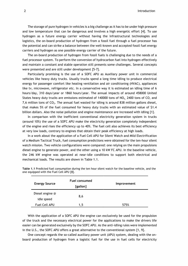
In a work about the application of a Fuel Cell APU for Silent Watch and Mild Electrification
of a Medium Tactical Truck, fuel consumption predictions were obtained for the ten-hour silent
watch mission. Two vehicle configurations were compared: one relying on the main propulsions
diesel engine to generate power, and the other using a 10 kW FC APU. In the baseline vehicle,
the 246 kW engine was operated at near-idle conditions to support both electrical and
mechanical loads. The results are shown in Table 1.1.
Table 1.1 Predicted fuel consumption during the ten hour silent watch for the baseline vehicle, and the one equipped with the Fuel Cell APU [8].
Energy Source Fuel consumed
[gallon] Improvement
Diesel engine @
idle speed 8,6
Fuel Cell APU 1,5 575%
With the application of a SOFC APU the engine can exclusively be used for the propulsion
of the truck and the necessary electrical power for the applications to make the drivers life
easier can be generated exclusively by the SOFC APU. As the anti-idling rules were implemented
in the U.S., the SOFC APU offers a great alternative to the conventional system [1, 9].
One concept regards the so-called auxiliary power unit (APU) system, dealing with the on-
board production of hydrogen from a logistic fuel for the use in fuel cells for electricity
Motivation 3
production in the power range of 3 - 4 kW. One of its crucial modules is the evaporation and
premixing chamber. The operation and optimisation of this module and the whole concept will
be explained further on and serve as the technical background for the experimental
investigations within this dissertation.
1.1. Motivation
AVL develops since 2002 auxiliary power units for trucks based on High-temperature fuel
cell technology (SOFC - Solid Oxide Fuel Cell) operated with conventional diesel. As part of the
work a concept for a Final realization was developed. A crucial subsystem in this concept is the
diesel fuel processing unit. From this (patented) arrangement is expected an improved system
start-up and also benefits during the operation by the Heat transfer between the burner, the
reformer and the premixing chamber that we will call an evaporation unit or simply an
evaporator throughout this dissertation.
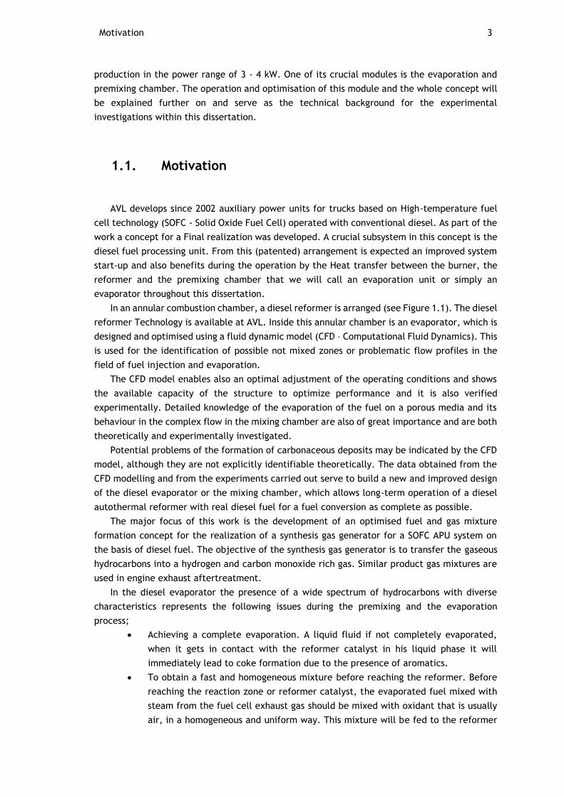
In an annular combustion chamber, a diesel reformer is arranged (see Figure 1.1). The diesel
reformer Technology is available at AVL. Inside this annular chamber is an evaporator, which is
designed and optimised using a fluid dynamic model (CFD – Computational Fluid Dynamics). This
is used for the identification of possible not mixed zones or problematic flow profiles in the
field of fuel injection and evaporation.
The CFD model enables also an optimal adjustment of the operating conditions and shows
the available capacity of the structure to optimize performance and it is also verified
experimentally. Detailed knowledge of the evaporation of the fuel on a porous media and its
behaviour in the complex flow in the mixing chamber are also of great importance and are both
theoretically and experimentally investigated.
Potential problems of the formation of carbonaceous deposits may be indicated by the CFD
model, although they are not explicitly identifiable theoretically. The data obtained from the
CFD modelling and from the experiments carried out serve to build a new and improved design
of the diesel evaporator or the mixing chamber, which allows long-term operation of a diesel
autothermal reformer with real diesel fuel for a fuel conversion as complete as possible.
The major focus of this work is the development of an optimised fuel and gas mixture
formation concept for the realization of a synthesis gas generator for a SOFC APU system on
the basis of diesel fuel. The objective of the synthesis gas generator is to transfer the gaseous
hydrocarbons into a hydrogen and carbon monoxide rich gas. Similar product gas mixtures are
used in engine exhaust aftertreatment.
In the diesel evaporator the presence of a wide spectrum of hydrocarbons with diverse
characteristics represents the following issues during the premixing and the evaporation
process;
Achieving a complete evaporation. A liquid fluid if not completely evaporated,
when it gets in contact with the reformer catalyst in his liquid phase it will
immediately lead to coke formation due to the presence of aromatics.
To obtain a fast and homogeneous mixture before reaching the reformer. Before
reaching the reaction zone or reformer catalyst, the evaporated fuel mixed with
steam from the fuel cell exhaust gas should be mixed with oxidant that is usually
air, in a homogeneous and uniform way. This mixture will be fed to the reformer
4 Introduction
to ensure constant inlet steam to carbon (S/C) and carbon to oxygen (C/O) ratios
required for a sustainable and stable hydrogen throughput. A local occurrence of
insufficient steam (low S/C ratios) and excess oxidant (low C/O ratios) can lead to
coke formation and unexpected temperature spikes.
Maintain a stable operation with an operational safety within the reformer. For
this requirement besides the uniform mixing a rapid and fast mixing is also required
because of the auto-ignition temperatures of n-decane that are smaller than their
boiling points. This is specific in processes involving oxygen and becomes critical
during evaporation of diesel
Figure 1.1 Concept sketch of the SOFC APU [10]
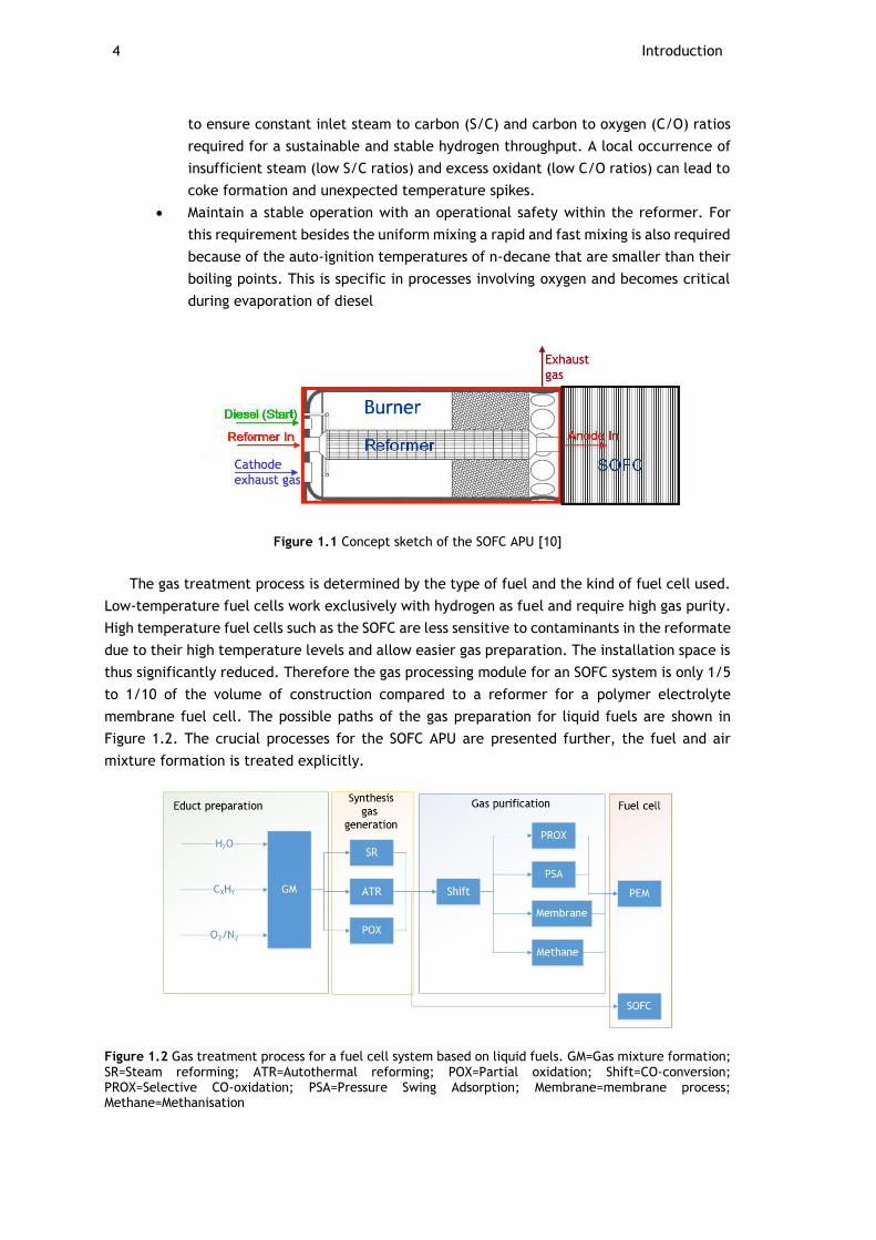
The gas treatment process is determined by the type of fuel and the kind of fuel cell used.
Low-temperature fuel cells work exclusively with hydrogen as fuel and require high gas purity.
High temperature fuel cells such as the SOFC are less sensitive to contaminants in the reformate
due to their high temperature levels and allow easier gas preparation. The installation space is
thus significantly reduced. Therefore the gas processing module for an SOFC system is only 1/5
to 1/10 of the volume of construction compared to a reformer for a polymer electrolyte
membrane fuel cell. The possible paths of the gas preparation for liquid fuels are shown in
Figure 1.2. The crucial processes for the SOFC APU are presented further, the fuel and air
mixture formation is treated explicitly.
Figure 1.2 Gas treatment process for a fuel cell system based on liquid fuels. GM=Gas mixture formation; SR=Steam reforming; ATR=Autothermal reforming; POX=Partial oxidation; Shift=CO-conversion; PROX=Selective CO-oxidation; PSA=Pressure Swing Adsorption; Membrane=membrane process; Methane=Methanisation
Goals of the dissertation 5
The methods applied to synthesis gas generation in this work are focused on the partial
oxidation (POX) and autothermal reforming (ATR). Both are suitable for direct coupling to a
high-temperature fuel cell. The ATR reformer can be coupled with downstream gas cleaning
with other fuel cells. In the SOFC technology complete conversion of hydrocarbons to H2 is not
needed. Unreacted methane, carbon monoxide and light hydrocarbons can be fed to the SOFC
anode with the hydrogen.
The requirements for the APU are mainly derived from the planned application in American
trucks. There, the APU will replace the banned engine idling of vehicles through the
conventional methods by the new legislation and provide uninterrupted electrical power for
the consumer. The heat released by the APU during power generation is also used to heat the
vehicle.
To ensure an economic efficiency of the APU, all components have to be designed for an
operating time of approximately 40,000 hours. During this time, neither maintenance nor
interferences should occur. In a continuous weekly operation of five days per week this
corresponds to a lifetime of about 6,5 years. During this time, around 340 full thermal cycles
should occur, that is in addition to vibration, the maximum load for all materials.
1.2. Goals of the dissertation
Summarized this work aimed for the accomplishment of the following objectives:
1. Understand the basic principles of fuel cells, burning and reforming technologies
2. Understand the functioning of the entire SOFC APU system and its main components
3. Specification of the requirements
4. Evaluation of an optimised evaporation and premixing technology
5. Design of an optimised evaporation unit
6. System CFD simulation and optimization of the design
7. System set up on an AVL test bench
8. Testing and validation of the results with the hardware on a test bench
9. Verification comparison of the previous system with the new system
1.3. Document Outline
This dissertation will discuss a redesign, an eventual technology upgrade and optimisation
of a diesel evaporation unit for a mobile SOFC APU to be applied in trucks. In the second chapter
the state of the art technologies used in fuel cells especially SOFC are reviewed, highlighting
the issues that are considered essential. A general explanation of the main fuel gas production
technologies for fuel cells, its basic concepts, requirements and also its applications in SOFC
APU especially for trucks is given. A fundamental description is made about the evaporation
process. The idea of a fuel cell system is explained emphasizing the AVL SOFC system addressing
the DE-1 Evaporator.
In the third chapter the physical parameters that affect the evaporation and mixture
formation system taking into account the requirements of the applications are referred. The
6 Introduction
operating range of the fuel processing system is simulated and further the evaporator is
redesigned and modelled using computational fluid dynamics.
In the fourth chapter the construction and implementation of a modular fuel processing
test setup and a diesel evaporation test system using optical measurement techniques is
described.
The fifth chapter deals with the commissioning and the operational procedures of the
constructed test setups. In this chapter the evaluation process of the measured data is reported
and discussed.
In the sixth and final chapter the conclusion about this work are drawn outlining the
completed tasks, the methods employed and the recommendation for future work. At last a
final solution is recommended for the implementation in the AVL SOFC APU.
1.4. Methodology
That in this work to be optimised, developed and elaborated evaporator should be firstly
simulated through CFD calculations, implemented and tested on its boundary conditions to find
out all its weaknesses and malfunctions. With the available DE-1 unit takes place a proof of
concept, which shows how far improvements are needed. Finally, a model should be designed
and built out of the results that will meet the requirements of the APU.
1.4.1. Hardware
In the fuel cell laboratory of AVL, the high temperature test bench was used to perform the
experiments. This test bench is intended for testing and development of fuel cells, reformers,
afterburners, heat exchangers, valves and sensors and systems formed from them. It can be
operated with air, nitrogen (N2), carbon dioxide (CO2), carbon monoxide (CO), hydrogen (H2),
hydrogen sulphide (H2S), methane (CH4) and natural gas. Also for the operation of a system
there is the possibility of feeding diesel or gasoline through pipelines to the test. It is possible
to deliver the media flow-or pressure-controlled, control the heating, to moisten and also to
cool down. The media can be heated up to 800°C.
1.4.1.1. AVL Visioscope
The AVL Visioscope as illustrated in Figure 1.3 is a state of the art image acquisition, analysis
and processing system through an infrared camera which was developed for applications in
internal combustion engines research and development.
Methodology 7
Figure 1.3 AVL Visioscope
The system consists of the following components:
Instrument Trolley
PC
22’’ flat screen
PCO PixelFly CCD (charge-coupled device) Camera
Set of connecting cables
Set of endoscopes
Oil and dust free air cooling system for endoscopes.
ZP91.00 water cooling system for endoscopes.
Further details are explained in section 4.2.2.
1.4.2. Software
In the following section the different types of software used are briefly described. For the
calculations of the reaction enthalpies, stoichiometry’s and other important parameters
(temperature, pressure, mass flow etc.) Matlab/Simulink was used. The required parts were
designed in PTC Creo Elements/Pro 5.0. For the fluid dynamic analysis the internal software of
AVL called AVL Fire was used for the pre- and post-processing and the equation solving.
1.4.2.1. Matlab/Simulink
Matlab/Simulink is a program system for solving numerical equations. It is represented in a
block diagram environment and enables multidomain simulation and Model-Based Design. It
supports various toolboxes and functions like system-level design, simulation, automatic code
generation, and continuous test and verification of embedded systems becoming so a very
versatile tool. There was also provided an internal fuel cell toolbox with all the main
components, modules and reactors of a fuel cell and a fuel processing system, enabling a
8 Introduction
precise overall numerical analysis of each functions, systems and modules, giving also the
opportunity to analyse numerically new designs and arrangements of the modules.
1.4.2.2. PTC Creo Elements/Pro 5.0
PTC Creo Elements/Pro is an integrated 3D CAD/CAM/CAE solution. It provides a complete
set of design analysis and manufacturing capabilities, all integrated in one platform. Some main
functions are solid modeling, surface rendering, data interoperability, routed systems design,
simulation, tolerance analysis, numerical control, tooling design, assembly modelling and
drafting and finite elements analysing. This software was used to create the complete 3D model
of some required parts. It was also provided a full 3D model of the entire solid oxide fuel cell
auxiliary power unit (SOFC APU), to be analysed and to study the integration of other possible
evaporator designs.
1.4.2.3. AVL Fire
FIRE is the internal software for fluid dynamic simulations. It provides a complete CFD
environment with different integrated tools for solving, pre- and post-processing applications
embedded in an intuitive GUI. The overall environment and individual components of Fire
enable so the application to any phase of a fluid dynamic development process. FIRE was
developed to meet the main requirements in the automotive research and development field,
allowing its users to adjust modeling complexity and to integrate the software into their CAx
framework.

Methodology 9

11
Chapter 2
State of the Art
2.1. Fuel Cell
2.1.1. Evolution
The origins of fuel cells are far behind, since the nineteenth century. The electrolysis
process is known since 1800 from the scientist William Nicholson and Johann Ritter that
decomposed water into hydrogen and oxygen. Later on, the British judge and scientist William
R. Grove succeeded in 1838 to reverse the electrolysis process to produce electric current
rather than use electric current and build the first fuel cell, which was referred to as "gas
battery" [11].
The term "fuel cell" was introduced in 1889 by the chemists Ludwig Mond and Charles Langer
[12]. The theoretical foundations of the fuel cell were created in 1893 by the work of Frederick
W. Ostwald. Over time, various kinds of fuel cells have been developed [13]. The first high
temperature fuel cell with solid electrolyte was introduced in 1937 by Emil Baur and Hans Price
[14]. Technical difficulties and high costs led to the termination of the project.
A new attempt for the development of the concept proposed by Davtyan in 1945 failed for
the same reasons [15]. The evolution of solid oxide fuel cells to its present state was mainly
driven forward by the work at the Westinghouse (USA), now Siemens-Westinghouse, which are
going on with their development since the 60s of the 20th Century [16].
2.1.2. Operation standard procedures
The kernel of a fuel cell is an ion-conducting electrolyte which separates the two mutually
reactive substances from each other. In most cases, these are hydrogen on one side and oxygen
on the other side. In some fuel cells can be used other fuels instead of hydrogen, such as CO,
methanol and hydrazine. The electrolyte has the property that it is permeable to the ionic
species of one of the reactants.
In the case of the SOFC, it deals with O2 ions. For electrons, the electrolyte is non-
conductive. Due to the concentration on both sides of the electrolyte, the ions migrate from
12 State of the Art
one side to the other. For this, the atoms or molecules of one of the gas have to be ionised,
that means they have to gain or lose electrons and are thus themselves electrically charged.
This process takes place at an electrode that supports the ionization process catalytically
and accomplishes the electron exchange. The electrode is connected on the other side of the
electrolyte of an electrical line with a counter electrode.
On the counter electrode, the charges transported through the ions are balanced again.
The molecules that reach from one side to the other then react with the molecules of the other
reactants to lower molecular weight substances, such as in the case of hydrogen and oxygen to
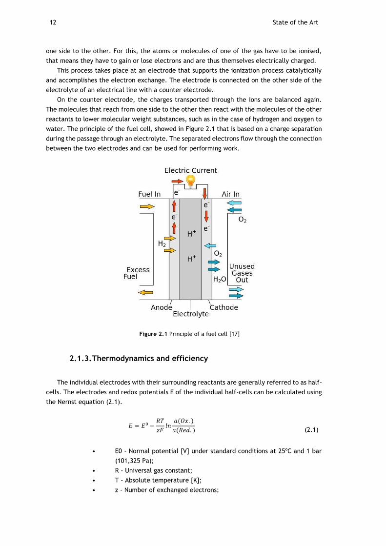
water. The principle of the fuel cell, showed in Figure 2.1 that is based on a charge separation
during the passage through an electrolyte. The separated electrons flow through the connection
between the two electrodes and can be used for performing work.
Figure 2.1 Principle of a fuel cell [17]
2.1.3. Thermodynamics and efficiency
The individual electrodes with their surrounding reactants are generally referred to as half-
cells. The electrodes and redox potentials E of the individual half-cells can be calculated using
the Nernst equation (2.1).
𝐸 = 𝐸0 −𝑅𝑇
𝑧𝐹𝑙𝑛
𝑎(𝑂𝑥. )
𝑎(𝑅𝑒𝑑. )
(2.1)
• E0 - Normal potential [V] under standard conditions at 25ºC and 1 bar
(101,325 Pa);
• R - Universal gas constant;
• T - Absolute temperature [K];
• z - Number of exchanged electrons;
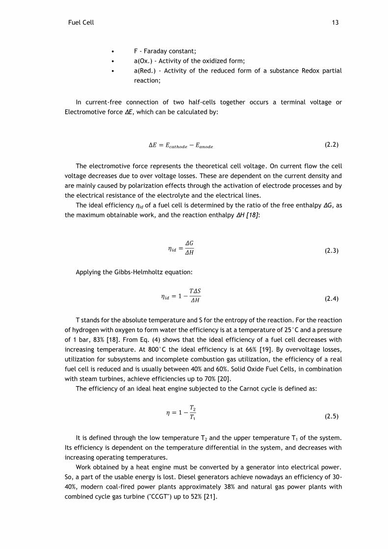
Fuel Cell 13
• F - Faraday constant;
• a(Ox.) - Activity of the oxidized form;
• a(Red.) - Activity of the reduced form of a substance Redox partial
reaction;
In current-free connection of two half-cells together occurs a terminal voltage or
Electromotive force ΔE, which can be calculated by:
∆𝐸 = 𝐸𝑐𝑎𝑡ℎ𝑜𝑑𝑒 − 𝐸𝑎𝑛𝑜𝑑𝑒 (2.2)
The electromotive force represents the theoretical cell voltage. On current flow the cell
voltage decreases due to over voltage losses. These are dependent on the current density and
are mainly caused by polarization effects through the activation of electrode processes and by
the electrical resistance of the electrolyte and the electrical lines.
The ideal efficiency ηid of a fuel cell is determined by the ratio of the free enthalpy ΔG, as
the maximum obtainable work, and the reaction enthalpy ΔH [18]:
𝜂𝑖𝑑 =𝛥𝐺
𝛥𝐻 (2.3)
Applying the Gibbs-Helmholtz equation:
𝜂𝑖𝑑 = 1 −𝑇𝛥𝑆
𝛥𝐻 (2.4)
T stands for the absolute temperature and S for the entropy of the reaction. For the reaction
of hydrogen with oxygen to form water the efficiency is at a temperature of 25°C and a pressure
of 1 bar, 83% [18]. From Eq. (4) shows that the ideal efficiency of a fuel cell decreases with
increasing temperature. At 800°C the ideal efficiency is at 66% [19]. By overvoltage losses,
utilization for subsystems and incomplete combustion gas utilization, the efficiency of a real
fuel cell is reduced and is usually between 40% and 60%. Solid Oxide Fuel Cells, in combination
with steam turbines, achieve efficiencies up to 70% [20].
The efficiency of an ideal heat engine subjected to the Carnot cycle is defined as:
𝜂 = 1 −𝑇2
𝑇1
(2.5)
It is defined through the low temperature T2 and the upper temperature T1 of the system.
Its efficiency is dependent on the temperature differential in the system, and decreases with
increasing operating temperatures.
Work obtained by a heat engine must be converted by a generator into electrical power.
So, a part of the usable energy is lost. Diesel generators achieve nowadays an efficiency of 30-
40%, modern coal-fired power plants approximately 38% and natural gas power plants with
combined cycle gas turbine ("CCGT") up to 52% [21].
14 State of the Art
2.1.4. Fuel Cell Types
The types of fuel cells available today differ mainly in the material of their electrolyte.
This also determines the appropriate operating temperature. Fuel cells can be roughly divided
into low, medium-and high-temperature cells. As low-temperature cells there are the alkaline
fuel cells (AFC), the polymer electrolyte membrane fuel cells (PEMFC) and direct methanol fuel
cell (DMFC).
The phosphoric acid fuel cell (PAFC) is a medium-temperature cell, whilst the molten
carbonate fuel cell (MCFC) and solid oxide fuel cells (SOFC) are high-temperature fuel cells.
Due to their high operating temperatures they are able to split, hydrocarbons, such as methane
or diesel, through the so-called internal reforming in H2 and CO2, which can be operated with
a variety of fuels. Table 2.1 gives an overview of the common types of fuel cells and their
applications.
2.1.5. The Solid Oxide Fuel Cell
The functional diagram can be seen in figure 2.2:
Figure 2.2 Functional diagram of the SOFC [22]
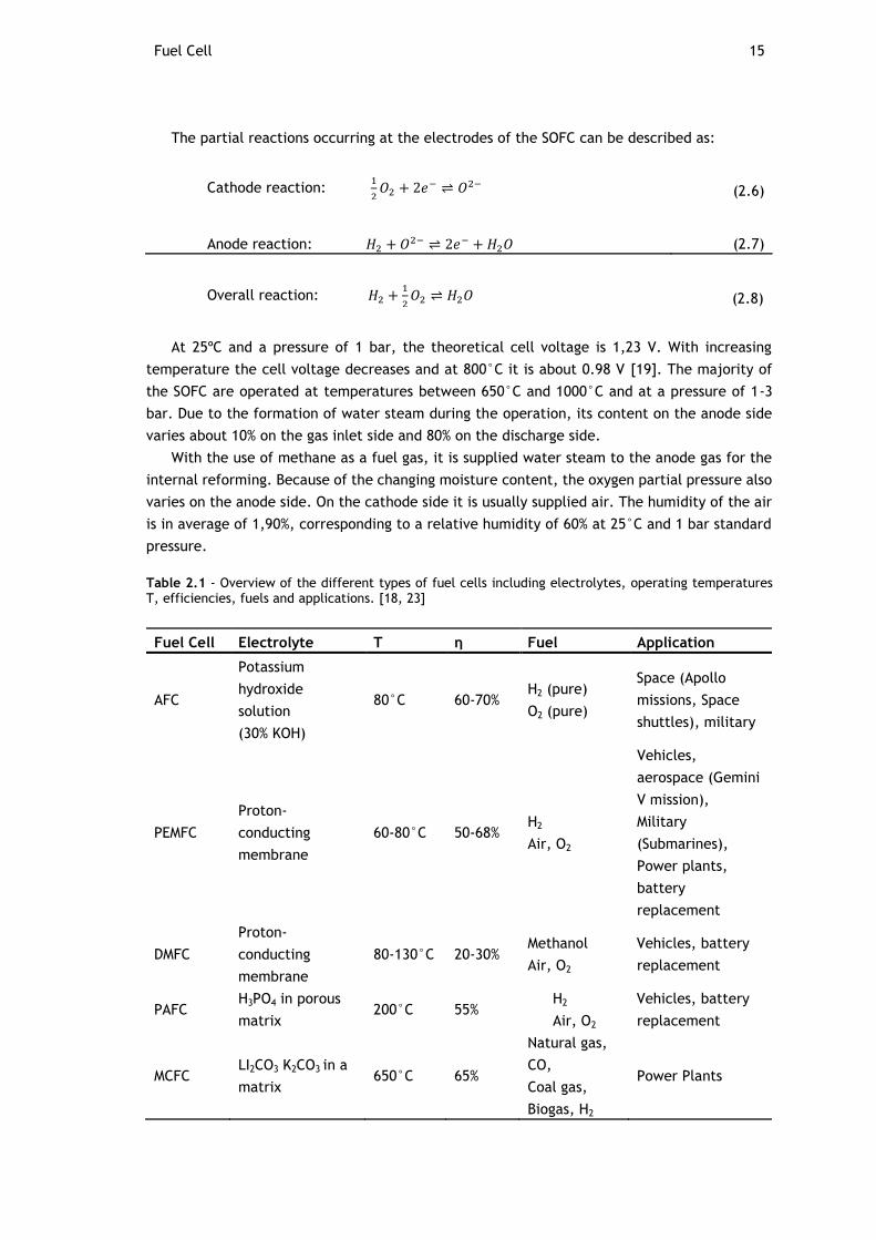
Fuel Cell 15
The partial reactions occurring at the electrodes of the SOFC can be described as:
Cathode reaction: 1
2𝑂2 + 2𝑒− ⇌ 𝑂2− (2.6)
Anode reaction: 𝐻2 + 𝑂2− ⇌ 2𝑒− + 𝐻2𝑂 (2.7)
Overall reaction: 𝐻2 +1
2𝑂2 ⇌ 𝐻2𝑂 (2.8)
At 25ºC and a pressure of 1 bar, the theoretical cell voltage is 1,23 V. With increasing
temperature the cell voltage decreases and at 800°C it is about 0.98 V [19]. The majority of
the SOFC are operated at temperatures between 650°C and 1000°C and at a pressure of 1-3
bar. Due to the formation of water steam during the operation, its content on the anode side
varies about 10% on the gas inlet side and 80% on the discharge side.
With the use of methane as a fuel gas, it is supplied water steam to the anode gas for the
internal reforming. Because of the changing moisture content, the oxygen partial pressure also
varies on the anode side. On the cathode side it is usually supplied air. The humidity of the air
is in average of 1,90%, corresponding to a relative humidity of 60% at 25°C and 1 bar standard
pressure.
Table 2.1 - Overview of the different types of fuel cells including electrolytes, operating temperatures T, efficiencies, fuels and applications. [18, 23]
Fuel Cell Electrolyte T η Fuel Application
AFC
Potassium
hydroxide
solution
(30% KOH)
80°C 60-70% H2 (pure)
O2 (pure)
Space (Apollo
missions, Space
shuttles), military
PEMFC
Proton-
conducting
membrane
60-80°C 50-68% H2
Air, O2
Vehicles,
aerospace (Gemini
V mission),
Military
(Submarines),
Power plants,
battery
replacement
DMFC
Proton-
conducting
membrane
80-130°C 20-30% Methanol
Air, O2
Vehicles, battery
replacement
PAFC H3PO4 in porous
matrix 200°C 55%
H2
Air, O2
Vehicles, battery
replacement
MCFC LI2CO3 K2CO3 in a
matrix 650°C 65%
Natural gas,
CO,
Coal gas,
Biogas, H2
Power Plants
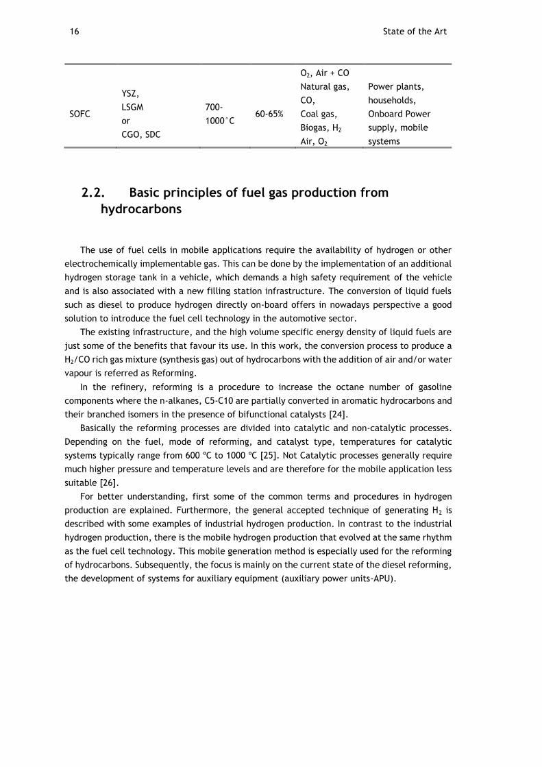
16 State of the Art
O2, Air + CO
SOFC
YSZ,
LSGM
or
CGO, SDC
700-
1000°C 60-65%
Natural gas,
CO,
Coal gas,
Biogas, H2
Air, O2
Power plants,
households,
Onboard Power
supply, mobile
systems
2.2. Basic principles of fuel gas production from
hydrocarbons
The use of fuel cells in mobile applications require the availability of hydrogen or other
electrochemically implementable gas. This can be done by the implementation of an additional
hydrogen storage tank in a vehicle, which demands a high safety requirement of the vehicle
and is also associated with a new filling station infrastructure. The conversion of liquid fuels
such as diesel to produce hydrogen directly on-board offers in nowadays perspective a good
solution to introduce the fuel cell technology in the automotive sector.
The existing infrastructure, and the high volume specific energy density of liquid fuels are
just some of the benefits that favour its use. In this work, the conversion process to produce a
H2/CO rich gas mixture (synthesis gas) out of hydrocarbons with the addition of air and/or water
vapour is referred as Reforming.
In the refinery, reforming is a procedure to increase the octane number of gasoline
components where the n-alkanes, C5-C10 are partially converted in aromatic hydrocarbons and
their branched isomers in the presence of bifunctional catalysts [24].
Basically the reforming processes are divided into catalytic and non-catalytic processes.
Depending on the fuel, mode of reforming, and catalyst type, temperatures for catalytic
systems typically range from 600 ºC to 1000 ºC [25]. Not Catalytic processes generally require
much higher pressure and temperature levels and are therefore for the mobile application less
suitable [26].
For better understanding, first some of the common terms and procedures in hydrogen
production are explained. Furthermore, the general accepted technique of generating H2 is
described with some examples of industrial hydrogen production. In contrast to the industrial
hydrogen production, there is the mobile hydrogen production that evolved at the same rhythm
as the fuel cell technology. This mobile generation method is especially used for the reforming
of hydrocarbons. Subsequently, the focus is mainly on the current state of the diesel reforming,
the development of systems for auxiliary equipment (auxiliary power units-APU).
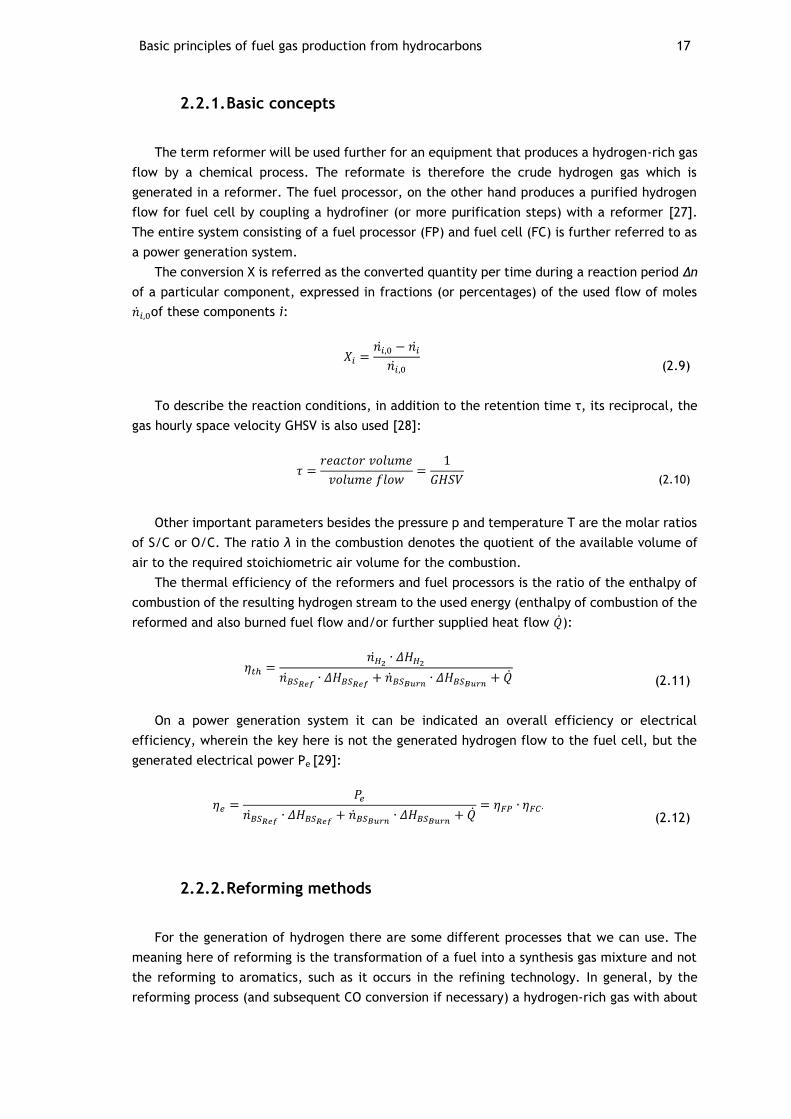
Basic principles of fuel gas production from hydrocarbons 17
2.2.1. Basic concepts
The term reformer will be used further for an equipment that produces a hydrogen-rich gas
flow by a chemical process. The reformate is therefore the crude hydrogen gas which is
generated in a reformer. The fuel processor, on the other hand produces a purified hydrogen
flow for fuel cell by coupling a hydrofiner (or more purification steps) with a reformer [27].
The entire system consisting of a fuel processor (FP) and fuel cell (FC) is further referred to as
a power generation system.
The conversion X is referred as the converted quantity per time during a reaction period Δn
of a particular component, expressed in fractions (or percentages) of the used flow of moles
�̇�𝑖,0of these components i:
𝑋𝑖 =𝑛�̇�,0 − 𝑛�̇�
𝑛�̇�,0
(2.9)
To describe the reaction conditions, in addition to the retention time τ, its reciprocal, the
gas hourly space velocity GHSV is also used [28]:
𝜏 =𝑟𝑒𝑎𝑐𝑡𝑜𝑟 𝑣𝑜𝑙𝑢𝑚𝑒
𝑣𝑜𝑙𝑢𝑚𝑒 𝑓𝑙𝑜𝑤=
1
𝐺𝐻𝑆𝑉
(2.10)
Other important parameters besides the pressure p and temperature T are the molar ratios
of S/C or O/C. The ratio λ in the combustion denotes the quotient of the available volume of
air to the required stoichiometric air volume for the combustion.
The thermal efficiency of the reformers and fuel processors is the ratio of the enthalpy of
combustion of the resulting hydrogen stream to the used energy (enthalpy of combustion of the
reformed and also burned fuel flow and/or further supplied heat flow �̇�):
𝜂𝑡ℎ =𝑛�̇�2
∙ 𝛥𝐻𝐻2
𝑛�̇�𝑆𝑅𝑒𝑓∙ 𝛥𝐻𝐵𝑆𝑅𝑒𝑓
+ �̇�𝐵𝑆𝐵𝑢𝑟𝑛∙ 𝛥𝐻𝐵𝑆𝐵𝑢𝑟𝑛
+ �̇�
(2.11)
On a power generation system it can be indicated an overall efficiency or electrical
efficiency, wherein the key here is not the generated hydrogen flow to the fuel cell, but the
generated electrical power Pe [29]:
𝜂𝑒 =𝑃𝑒
𝑛�̇�𝑆𝑅𝑒𝑓∙ 𝛥𝐻𝐵𝑆𝑅𝑒𝑓
+ �̇�𝐵𝑆𝐵𝑢𝑟𝑛∙ 𝛥𝐻𝐵𝑆𝐵𝑢𝑟𝑛
+ �̇�= 𝜂𝐹𝑃 ∙ 𝜂𝐹𝐶∙
(2.12)
2.2.2. Reforming methods
For the generation of hydrogen there are some different processes that we can use. The
meaning here of reforming is the transformation of a fuel into a synthesis gas mixture and not
the reforming to aromatics, such as it occurs in the refining technology. In general, by the
reforming process (and subsequent CO conversion if necessary) a hydrogen-rich gas with about
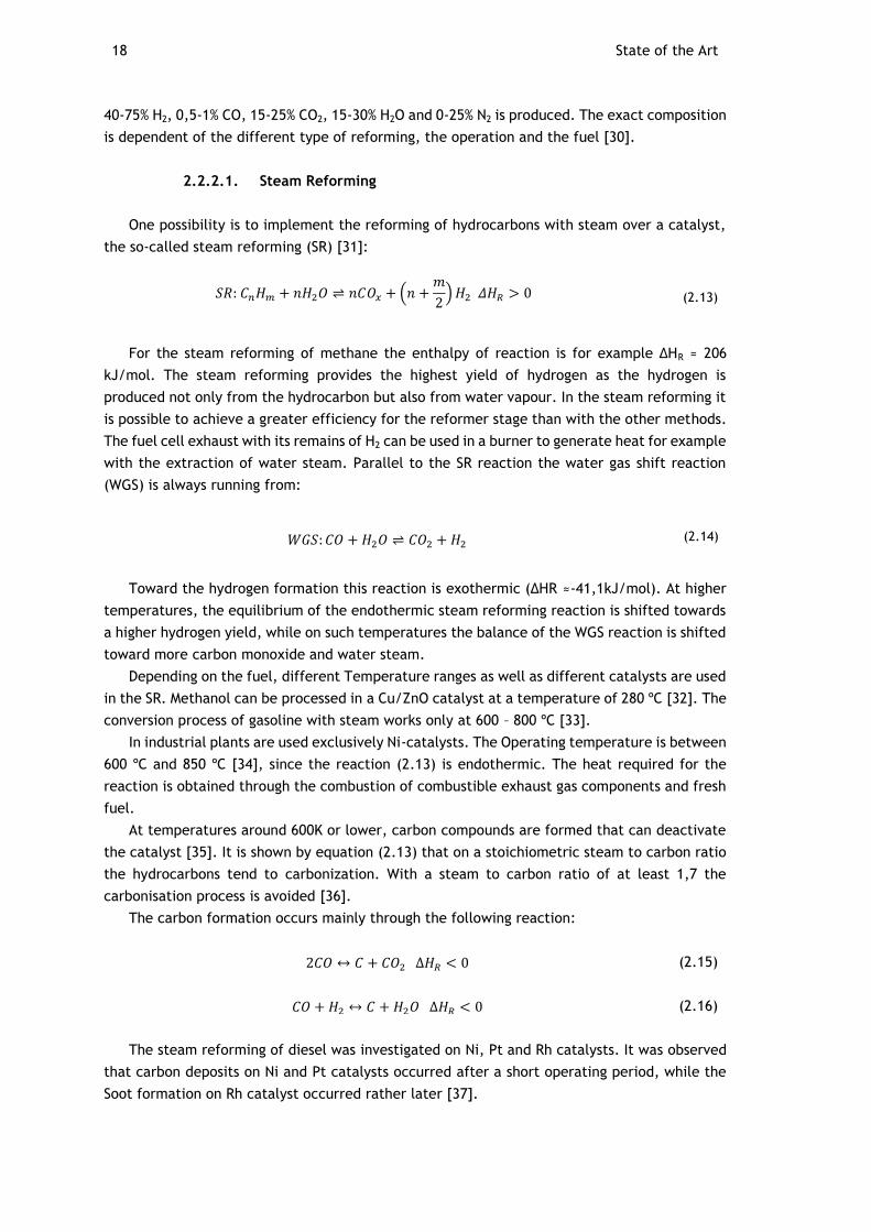
18 State of the Art
40-75% H2, 0,5-1% CO, 15-25% CO2, 15-30% H2O and 0-25% N2 is produced. The exact composition
is dependent of the different type of reforming, the operation and the fuel [30].
2.2.2.1. Steam Reforming
One possibility is to implement the reforming of hydrocarbons with steam over a catalyst,
the so-called steam reforming (SR) [31]:
𝑆𝑅: 𝐶𝑛𝐻𝑚 + 𝑛𝐻2𝑂 ⇌ 𝑛𝐶𝑂𝑥 + (𝑛 +𝑚
2) 𝐻2 𝛥𝐻𝑅 > 0 (2.13)
For the steam reforming of methane the enthalpy of reaction is for example ΔHR ≈ 206
kJ/mol. The steam reforming provides the highest yield of hydrogen as the hydrogen is
produced not only from the hydrocarbon but also from water vapour. In the steam reforming it
is possible to achieve a greater efficiency for the reformer stage than with the other methods.
The fuel cell exhaust with its remains of H2 can be used in a burner to generate heat for example
with the extraction of water steam. Parallel to the SR reaction the water gas shift reaction
(WGS) is always running from:
𝑊𝐺𝑆: 𝐶𝑂 + 𝐻2𝑂 ⇌ 𝐶𝑂2 + 𝐻2 (2.14)
Toward the hydrogen formation this reaction is exothermic (ΔHR ≈-41,1kJ/mol). At higher
temperatures, the equilibrium of the endothermic steam reforming reaction is shifted towards
a higher hydrogen yield, while on such temperatures the balance of the WGS reaction is shifted
toward more carbon monoxide and water steam.
Depending on the fuel, different Temperature ranges as well as different catalysts are used
in the SR. Methanol can be processed in a Cu/ZnO catalyst at a temperature of 280 ºC [32]. The
conversion process of gasoline with steam works only at 600 – 800 ºC [33].
In industrial plants are used exclusively Ni-catalysts. The Operating temperature is between
600 ºC and 850 ºC [34], since the reaction (2.13) is endothermic. The heat required for the
reaction is obtained through the combustion of combustible exhaust gas components and fresh
fuel.
At temperatures around 600K or lower, carbon compounds are formed that can deactivate
the catalyst [35]. It is shown by equation (2.13) that on a stoichiometric steam to carbon ratio
the hydrocarbons tend to carbonization. With a steam to carbon ratio of at least 1,7 the
carbonisation process is avoided [36].
The carbon formation occurs mainly through the following reaction:
2𝐶𝑂 ↔ 𝐶 + 𝐶𝑂2 ∆𝐻𝑅 < 0 (2.15)
𝐶𝑂 + 𝐻2 ↔ 𝐶 + 𝐻2𝑂 ∆𝐻𝑅 < 0 (2.16)
The steam reforming of diesel was investigated on Ni, Pt and Rh catalysts. It was observed
that carbon deposits on Ni and Pt catalysts occurred after a short operating period, while the
Soot formation on Rh catalyst occurred rather later [37].
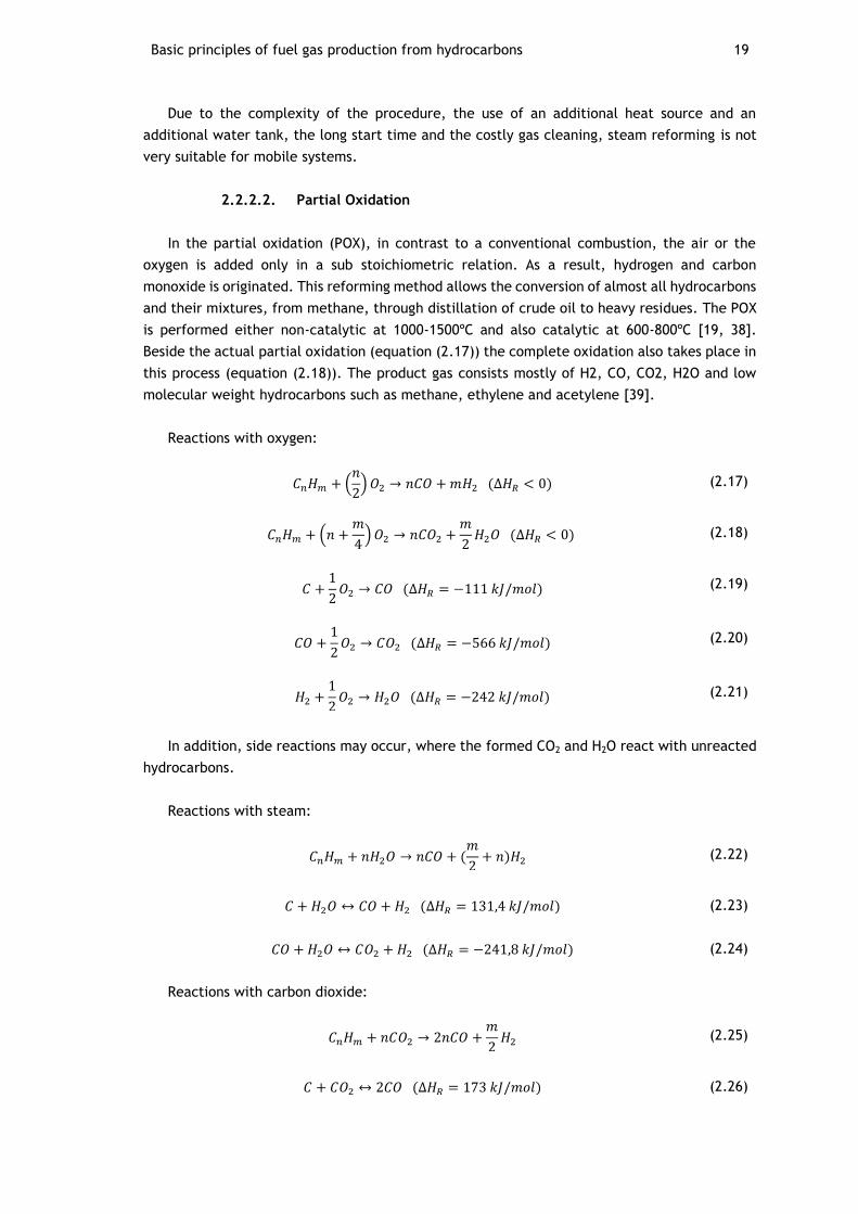
Basic principles of fuel gas production from hydrocarbons 19
Due to the complexity of the procedure, the use of an additional heat source and an
additional water tank, the long start time and the costly gas cleaning, steam reforming is not
very suitable for mobile systems.
2.2.2.2. Partial Oxidation
In the partial oxidation (POX), in contrast to a conventional combustion, the air or the
oxygen is added only in a sub stoichiometric relation. As a result, hydrogen and carbon
monoxide is originated. This reforming method allows the conversion of almost all hydrocarbons
and their mixtures, from methane, through distillation of crude oil to heavy residues. The POX
is performed either non-catalytic at 1000-1500ºC and also catalytic at 600-800ºC [19, 38].
Beside the actual partial oxidation (equation (2.17)) the complete oxidation also takes place in
this process (equation (2.18)). The product gas consists mostly of H2, CO, CO2, H2O and low
molecular weight hydrocarbons such as methane, ethylene and acetylene [39].
Reactions with oxygen:
𝐶𝑛𝐻𝑚 + (𝑛
2) 𝑂2 → 𝑛𝐶𝑂 + 𝑚𝐻2 (∆𝐻𝑅 < 0) (2.17)
𝐶𝑛𝐻𝑚 + (𝑛 +𝑚
4) 𝑂2 → 𝑛𝐶𝑂2 +
𝑚
2𝐻2𝑂 (∆𝐻𝑅 < 0) (2.18)
𝐶 +1
2𝑂2 → 𝐶𝑂 (∆𝐻𝑅 = −111 𝑘𝐽/𝑚𝑜𝑙) (2.19)
𝐶𝑂 +1
2𝑂2 → 𝐶𝑂2 (∆𝐻𝑅 = −566 𝑘𝐽/𝑚𝑜𝑙) (2.20)
𝐻2 +1
2𝑂2 → 𝐻2𝑂 (∆𝐻𝑅 = −242 𝑘𝐽/𝑚𝑜𝑙) (2.21)
In addition, side reactions may occur, where the formed CO2 and H2O react with unreacted
hydrocarbons.
Reactions with steam:
𝐶𝑛𝐻𝑚 + 𝑛𝐻2𝑂 → 𝑛𝐶𝑂 + (𝑚
2+ 𝑛)𝐻2 (2.22)
𝐶 + 𝐻2𝑂 ↔ 𝐶𝑂 + 𝐻2 (∆𝐻𝑅 = 131,4 𝑘𝐽/𝑚𝑜𝑙) (2.23)
𝐶𝑂 + 𝐻2𝑂 ↔ 𝐶𝑂2 + 𝐻2 (∆𝐻𝑅 = −241,8 𝑘𝐽/𝑚𝑜𝑙) (2.24)
Reactions with carbon dioxide:
𝐶𝑛𝐻𝑚 + 𝑛𝐶𝑂2 → 2𝑛𝐶𝑂 +𝑚
2𝐻2 (2.25)
𝐶 + 𝐶𝑂2 ↔ 2𝐶𝑂 (∆𝐻𝑅 = 173 𝑘𝐽/𝑚𝑜𝑙) (2.26)
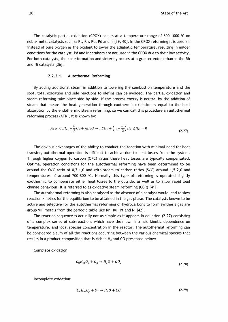
20 State of the Art
The catalytic partial oxidation (CPOX) occurs at a temperature range of 600-1000 ºC on
noble metal catalysts such as Pt, Rh, Ru, Pd and Ir [39, 40]. In the CPOX reforming it is used air
instead of pure oxygen as the oxidant to lower the adiabatic temperature, resulting in milder
conditions for the catalyst. Pd and Ir catalysts are not used in the CPOX due to their low activity.
For both catalysts, the coke formation and sintering occurs at a greater extent than in the Rh
and Ni catalysts [36].
2.2.2.1. Autothermal Reforming
By adding additional steam in addition to lowering the combustion temperature and the
soot, total oxidation and side reactions to olefins can be avoided. The partial oxidation and
steam reforming take place side by side. If the process energy is neutral by the addition of
steam that means the heat generation through exothermic oxidation is equal to the heat
absorption by the endothermic steam reforming, so we can call this procedure an autothermal
reforming process (ATR), it is known by:
𝐴𝑇𝑅: 𝐶𝑛𝐻𝑚 +𝑛
2𝑂2 + 𝑛𝐻2𝑂 → 𝑛𝐶𝑂2 + (𝑛 +
𝑚
2) 𝐻2 𝛥𝐻𝑅 = 0
(2.27)
The obvious advantages of the ability to conduct the reaction with minimal need for heat
transfer, autothermal operation is difficult to achieve due to heat losses from the system.
Through higher oxygen to carbon (O/C) ratios these heat losses are typically compensated.
Optimal operation conditions for the autothermal reforming have been determined to be
around the O/C ratio of 0,7-1,0 and with steam to carbon ratios (S/C) around 1,5-2,0 and
temperatures of around 700-800 ºC. Normally this type of reforming is operated slightly
exothermic to compensate either heat losses to the outside, as well as to allow rapid load
change behaviour. It is referred to as oxidative steam reforming (OSR) [41].
The autothermal reforming is also catalysed as the absence of a catalyst would lead to slow
reaction kinetics for the equilibrium to be attained in the gas phase. The catalysts known to be
active and selective for the autothermal reforming of hydrocarbons to form synthesis gas are
group VIII metals from the periodic table like Rh, Ru, Pt and Ni [42].
The reaction sequence is actually not as simple as it appears in equation (2.27) consisting
of a complex series of sub-reactions which have their own intrinsic kinetic dependence on
temperature, and local species concentration in the reactor. The autothermal reforming can
be considered a sum of all the reactions occurring between the various chemical species that
results in a product composition that is rich in H2 and CO presented below:
Complete oxidation:
𝐶𝑛𝐻𝑚𝑂𝑝 + 𝑂2 → 𝐻2𝑂 + 𝐶𝑂2
(2.28)
Incomplete oxidation:
𝐶𝑛𝐻𝑚𝑂𝑝 + 𝑂2 → 𝐻2𝑂 + 𝐶𝑂 (2.29)
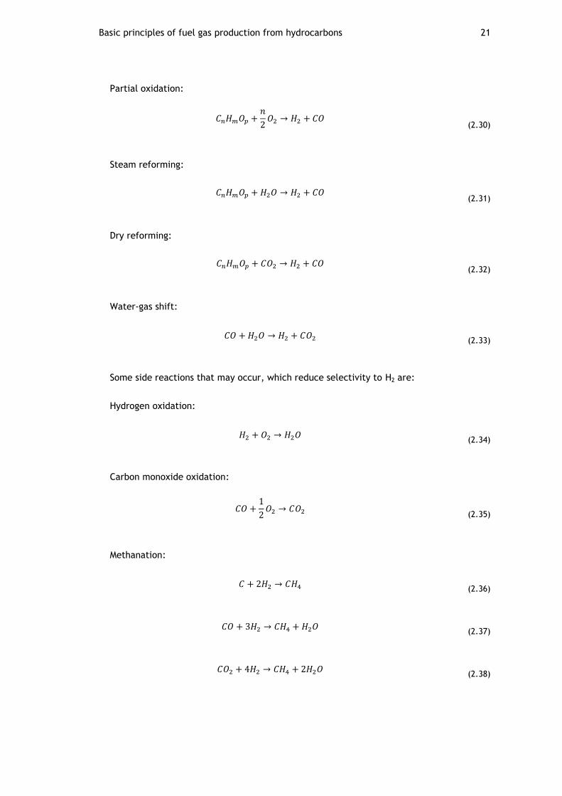
Basic principles of fuel gas production from hydrocarbons 21
Partial oxidation:
𝐶𝑛𝐻𝑚𝑂𝑝 +𝑛
2𝑂2 → 𝐻2 + 𝐶𝑂
(2.30)
Steam reforming:
𝐶𝑛𝐻𝑚𝑂𝑝 + 𝐻2𝑂 → 𝐻2 + 𝐶𝑂
(2.31)
Dry reforming:
𝐶𝑛𝐻𝑚𝑂𝑝 + 𝐶𝑂2 → 𝐻2 + 𝐶𝑂
(2.32)
Water-gas shift:
𝐶𝑂 + 𝐻2𝑂 → 𝐻2 + 𝐶𝑂2
(2.33)
Some side reactions that may occur, which reduce selectivity to H2 are:
Hydrogen oxidation:
𝐻2 + 𝑂2 → 𝐻2𝑂
(2.34)
Carbon monoxide oxidation:
𝐶𝑂 +1
2𝑂2 → 𝐶𝑂2
(2.35)
Methanation:
𝐶 + 2𝐻2 → 𝐶𝐻4
(2.36)
𝐶𝑂 + 3𝐻2 → 𝐶𝐻4 + 𝐻2𝑂
(2.37)
𝐶𝑂2 + 4𝐻2 → 𝐶𝐻4 + 2𝐻2𝑂
(2.38)
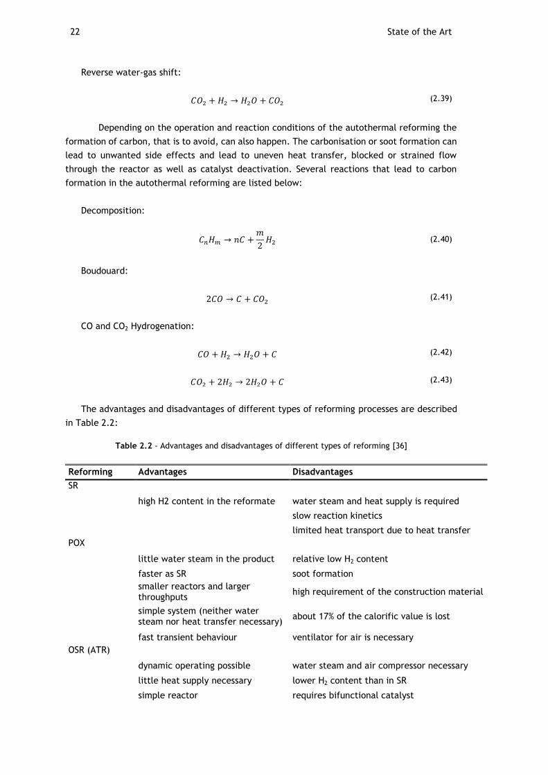
22 State of the Art
Reverse water-gas shift:
𝐶𝑂2 + 𝐻2 → 𝐻2𝑂 + 𝐶𝑂2 (2.39)
Depending on the operation and reaction conditions of the autothermal reforming the
formation of carbon, that is to avoid, can also happen. The carbonisation or soot formation can
lead to unwanted side effects and lead to uneven heat transfer, blocked or strained flow
through the reactor as well as catalyst deactivation. Several reactions that lead to carbon
formation in the autothermal reforming are listed below:
Decomposition:
𝐶𝑛𝐻𝑚 → 𝑛𝐶 +𝑚
2𝐻2 (2.40)
Boudouard:
2𝐶𝑂 → 𝐶 + 𝐶𝑂2 (2.41)
CO and CO2 Hydrogenation:
𝐶𝑂 + 𝐻2 → 𝐻2𝑂 + 𝐶 (2.42)
𝐶𝑂2 + 2𝐻2 → 2𝐻2𝑂 + 𝐶 (2.43)
The advantages and disadvantages of different types of reforming processes are described
in Table 2.2:
Table 2.2 - Advantages and disadvantages of different types of reforming [36]
Reforming Advantages Disadvantages
SR
high H2 content in the reformate water steam and heat supply is required
slow reaction kinetics
limited heat transport due to heat transfer
POX
little water steam in the product relative low H2 content
faster as SR soot formation
smaller reactors and larger throughputs
high requirement of the construction material
simple system (neither water steam nor heat transfer necessary)
about 17% of the calorific value is lost
fast transient behaviour ventilator for air is necessary
OSR (ATR)
dynamic operating possible water steam and air compressor necessary
little heat supply necessary lower H2 content than in SR
simple reactor requires bifunctional catalyst
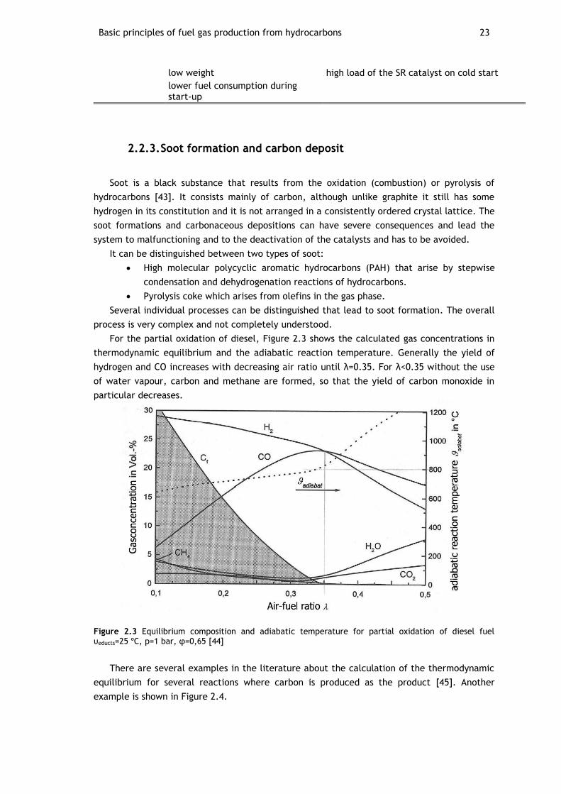
Basic principles of fuel gas production from hydrocarbons 23
low weight high load of the SR catalyst on cold start
lower fuel consumption during start-up
2.2.3. Soot formation and carbon deposit
Soot is a black substance that results from the oxidation (combustion) or pyrolysis of
hydrocarbons [43]. It consists mainly of carbon, although unlike graphite it still has some
hydrogen in its constitution and it is not arranged in a consistently ordered crystal lattice. The
soot formations and carbonaceous depositions can have severe consequences and lead the
system to malfunctioning and to the deactivation of the catalysts and has to be avoided.
It can be distinguished between two types of soot:
High molecular polycyclic aromatic hydrocarbons (PAH) that arise by stepwise
condensation and dehydrogenation reactions of hydrocarbons.
Pyrolysis coke which arises from olefins in the gas phase.
Several individual processes can be distinguished that lead to soot formation. The overall
process is very complex and not completely understood.
For the partial oxidation of diesel, Figure 2.3 shows the calculated gas concentrations in
thermodynamic equilibrium and the adiabatic reaction temperature. Generally the yield of
hydrogen and CO increases with decreasing air ratio until λ=0.35. For λ<0.35 without the use
of water vapour, carbon and methane are formed, so that the yield of carbon monoxide in
particular decreases.
Figure 2.3 Equilibrium composition and adiabatic temperature for partial oxidation of diesel fuel υeducts=25 ºC, p=1 bar, φ=0,65 [44]
There are several examples in the literature about the calculation of the thermodynamic
equilibrium for several reactions where carbon is produced as the product [45]. Another
example is shown in Figure 2.4.
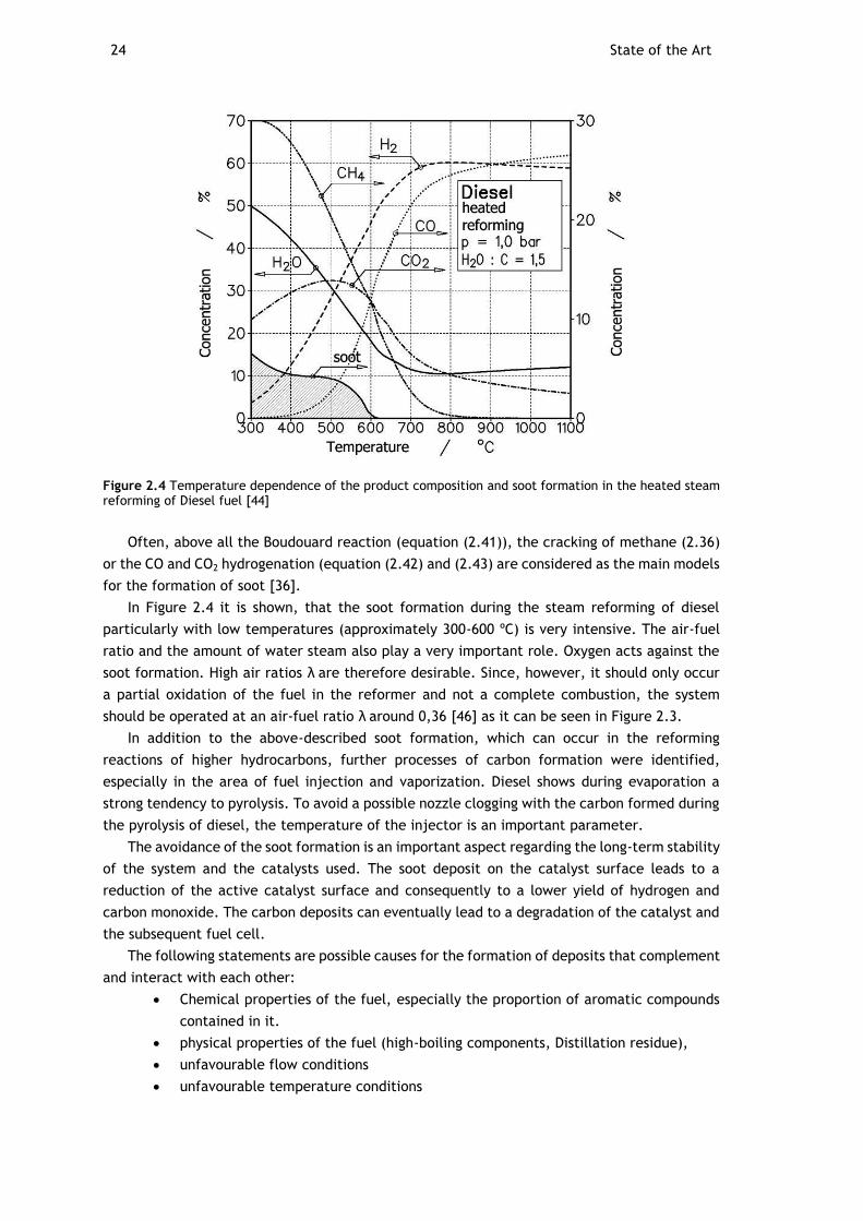
24 State of the Art
Figure 2.4 Temperature dependence of the product composition and soot formation in the heated steam reforming of Diesel fuel [44]
Often, above all the Boudouard reaction (equation (2.41)), the cracking of methane (2.36)
or the CO and CO2 hydrogenation (equation (2.42) and (2.43) are considered as the main models
for the formation of soot [36].
In Figure 2.4 it is shown, that the soot formation during the steam reforming of diesel
particularly with low temperatures (approximately 300-600 ºC) is very intensive. The air-fuel
ratio and the amount of water steam also play a very important role. Oxygen acts against the
soot formation. High air ratios λ are therefore desirable. Since, however, it should only occur
a partial oxidation of the fuel in the reformer and not a complete combustion, the system
should be operated at an air-fuel ratio λ around 0,36 [46] as it can be seen in Figure 2.3.
In addition to the above-described soot formation, which can occur in the reforming
reactions of higher hydrocarbons, further processes of carbon formation were identified,
especially in the area of fuel injection and vaporization. Diesel shows during evaporation a
strong tendency to pyrolysis. To avoid a possible nozzle clogging with the carbon formed during
the pyrolysis of diesel, the temperature of the injector is an important parameter.
The avoidance of the soot formation is an important aspect regarding the long-term stability
of the system and the catalysts used. The soot deposit on the catalyst surface leads to a
reduction of the active catalyst surface and consequently to a lower yield of hydrogen and
carbon monoxide. The carbon deposits can eventually lead to a degradation of the catalyst and
the subsequent fuel cell.
The following statements are possible causes for the formation of deposits that complement
and interact with each other:
Chemical properties of the fuel, especially the proportion of aromatic compounds
contained in it.
physical properties of the fuel (high-boiling components, Distillation residue),
unfavourable flow conditions
unfavourable temperature conditions
Basic principles of fuel gas production from hydrocarbons 25
In order to prevent carburization, during operation the O/C ratio has to be set as high as
possible. This can be achieved by the following measures:
Use of steam: the higher hydrocarbons are reformed with the water vapour
contained in the anode exhaust gas according to equation (2.31). If carbon deposits
are produced, this can be gasified with steam again according to equation (2.23).
Use of carbon dioxide: by increasing the partial pressure of carbon dioxide carbon
deposits could be gasified again according to equation (2.26).
Increase slightly the air-fuel ratio.
The actions mentioned above can be used in a SOFC APU system based on diesel by the
recirculation of the anode exhaust gas (product gas of the fuel cell of the electro-chemical
reaction of the reformate gas) having a high proportion of CO2 and H2O. This concept is already
in use by some system developers and it was also applied in the AVL SOFC APU and can be found
in some literature [36].
In addition through the recirculation of anode exhaust gas the fraction of inert gas is
increased and the temperature on the catalyst is decreased. Thus, an increase of the air ratio
λ at a constant temperature would be possible.
2.2.4. Reformers for Fuel Cells
Fuel cells require a hydrogen rich gas as fuel. There are basically two possibilities for the
mobile sector: to produce this hydrogen-rich gas or hydrogen stationary (on-site) and then save
it or to produce it locally (on-board) from conventional fuels (fuel gas production) and supply
it directly into the fuel cell. In hydrogen storage the following not yet overcomed problems
arise: The large amount of storage volumes due to the low energy density of hydrogen, the
safety aspects and the setup of a new hydrogen infrastructure for hydrogen storage [47].
2.2.4.1. Diesel Reformer
Basically a diesel reformer of a fuel cell power generation system should ensure [48]:
Low costs,
High efficiency,
Long periods of operation without maintenance and
Acceptable cold start and load change behaviour.
For long operation periods without maintenance soot formation during the reforming
process has to be avoided especially during the cold starts of the system [49]. A certain sulphur
tolerance of the catalyst has also a positive effect on its lifetime.
The partial oxidation has the greatest tendency to soot formation, especially at higher
hydrocarbons. During the evaporation of diesel or mixture with air, beside the soot formation
self-ignition can also occur. The Steam reforming is more susceptible to soot formation and
deposition compared to the ATR due to the simultaneous feed of air and steam in the ATR. To
avoid the formation of soot on the catalyst the steam-to-carbon ratio must be set as high as
possible in the SR and ATR. In the SR a steam-to-carbon ratio of 3 and in the ATR a steam to
carbon of 2,25 is recommended in [19, 50].
26 State of the Art
2.2.4.2. Reformer for Auxiliary Power Unit
For the provision of electricity and heat in mobile systems on-board power generators (APU)
can be used, which produce energy based on fuel cells. Depending on the application different
fuels based on hydrocarbon are advantageous:
Motor vehicles: in trucks and commercial vehicles diesel is available, in passenger
cars petrol or diesel is available;
In caravans or yachts: LPG (Liquefied Pressurised gas, propane/Bhutan) is already
available for cooking or heating purpose;
On ships diesel oil is available;
On aircraft kerosene fuel could be used [51, 52].
The advantages and requirements for the use of fuel cell APU in trucks are explained further
in more detail: On-board power is used either for the conditioning of the transport load
(cooling, heating) and also for the driver comfort (air conditioning, coffee maker, multimedia
etc.). In the USA the idle engine operation for on-board power generation makes an average of
20-40% of the entire truck engine running time. This is about six hours of engine operation at
an idle state per day [48]. The Environmental Protection Agency (EPA) and the U.S. Department
of Energy (DOE) are currently promoting programs to reduce these times and its resulting
emissions from the idling operation [53, 54]. Since the engine at idle state only has an efficiency
of about 10% and the alternator has an efficiency of about 30%, the overall efficiency results is
only 3% for the on-board power generation from diesel [51].
Electricity generation regardless of the engine operation appears therefore very promising.
There are already available ways to avoid idling operation to generate electricity, such as
batteries or backup generators, which have found only limited acceptance in the market. With
power generators, there is a problem especially in their weight and the resulting noise. A fuel
cell APU thus has the potential to reduce greenhouse emissions, costs [48], and has a
significantly better energy efficiency by saving on fuel as well as to increase operator comfort
and safety.
The low vibrations and noise emissions in the APU operation enable a better sleep and
decrease the fatigue of the driver. In addition, fuel cells are characterized by the fact that
their efficiency at part load operation in opposition to diesel engines does not drop [55].
Complete APU systems with reformer unit should achieve an efficiency of at least 30%, wherein
whole reformer unit with the purification of the reformate should have a theoretical efficiency
of 86% to 96% depending on the assumptions used in steam reforming [50, 56]. However, the
technical challenges are considerable [57]:
Stability against vibrations and bumps in the road,
Necessary reduction in the sulphur content to about 10ppm sulphur in diesel,
Optimization of the construction volume and weight,
Efficient thermal integration and interconnection,
A required power modulation of 1:10,
Short start-up time and high dynamics,
Tolerance to frequent starts and shutdowns
Low cost.
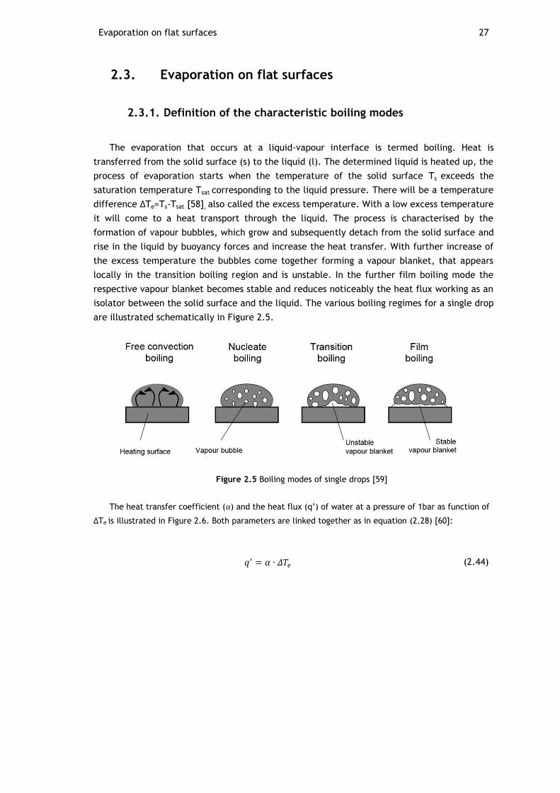
Evaporation on flat surfaces 27
2.3. Evaporation on flat surfaces
2.3.1. Definition of the characteristic boiling modes
The evaporation that occurs at a liquid-vapour interface is termed boiling. Heat is
transferred from the solid surface (s) to the liquid (l). The determined liquid is heated up, the
process of evaporation starts when the temperature of the solid surface Ts exceeds the
saturation temperature Tsat corresponding to the liquid pressure. There will be a temperature
difference ΔTe=Ts-Tsat [58], also called the excess temperature. With a low excess temperature
it will come to a heat transport through the liquid. The process is characterised by the
formation of vapour bubbles, which grow and subsequently detach from the solid surface and
rise in the liquid by buoyancy forces and increase the heat transfer. With further increase of
the excess temperature the bubbles come together forming a vapour blanket, that appears
locally in the transition boiling region and is unstable. In the further film boiling mode the
respective vapour blanket becomes stable and reduces noticeably the heat flux working as an
isolator between the solid surface and the liquid. The various boiling regimes for a single drop
are illustrated schematically in Figure 2.5.
Figure 2.5 Boiling modes of single drops [59]
The heat transfer coefficient (α) and the heat flux (q’) of water at a pressure of 1bar as function of
ΔTe is illustrated in Figure 2.6. Both parameters are linked together as in equation (2.28) [60]:
𝑞′ = 𝛼 ∙ 𝛥𝑇𝑒 (2.44)
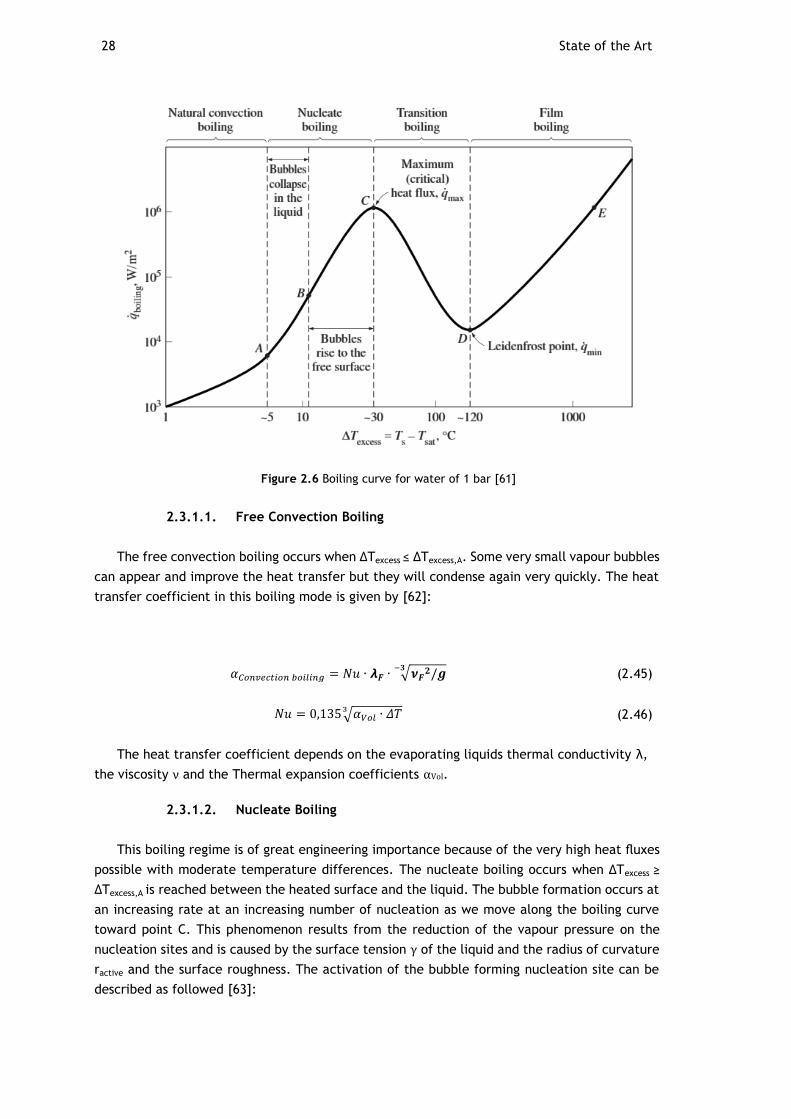
28 State of the Art
Figure 2.6 Boiling curve for water of 1 bar [61]
2.3.1.1. Free Convection Boiling
The free convection boiling occurs when ΔTexcess ≤ ΔTexcess,A. Some very small vapour bubbles
can appear and improve the heat transfer but they will condense again very quickly. The heat
transfer coefficient in this boiling mode is given by [62]:
𝛼𝐶𝑜𝑛𝑣𝑒𝑐𝑡𝑖𝑜𝑛 𝑏𝑜𝑖𝑙𝑖𝑛𝑔 = 𝑁𝑢 ∙ 𝞴𝑭 ∙ √𝝂𝑭𝟐/𝒈
−𝟑 (2.45)
𝑁𝑢 = 0,135 √𝛼𝑉𝑜𝑙 ∙ 𝛥𝑇3 (2.46)
The heat transfer coefficient depends on the evaporating liquids thermal conductivity λ,
the viscosity ν and the Thermal expansion coefficients αVol.
2.3.1.2. Nucleate Boiling
This boiling regime is of great engineering importance because of the very high heat fluxes
possible with moderate temperature differences. The nucleate boiling occurs when ΔTexcess ≥
ΔTexcess,A is reached between the heated surface and the liquid. The bubble formation occurs at
an increasing rate at an increasing number of nucleation as we move along the boiling curve
toward point C. This phenomenon results from the reduction of the vapour pressure on the
nucleation sites and is caused by the surface tension γ of the liquid and the radius of curvature
ractive and the surface roughness. The activation of the bubble forming nucleation site can be
described as followed [63]:
Evaporation on flat surfaces 29
𝑟𝑎𝑐𝑡𝑖𝑣𝑒 ≥2 ∙ 𝛾 ∙ 𝑇𝑠𝑎𝑡
𝜌𝑓 ∙ 𝛥ℎ𝑣 ∙ 𝛥𝑇𝑒𝑥𝑐𝑒𝑠𝑠
(2.47)
At point A of the boiling curve the first bubbles start forming at various preferential sites
on the heating surface. As the curve tends to point C the bubbles form at an increasing rate at
an increasing number of nucleation sites.
In the region A-B, isolated bubbles are formed on various preferential nucleation sites on
the heated surface. These bubbles are dissipated in the liquid shortly after they separate from
the solid surface. The free space caused by the bubbles is filled by the liquid in the vicinity of
the heater surface and the process is repeated. The dynamic agitation caused by the
entrainment of the liquid to the heater surface is primarily responsible for the increased heat
transfer coefficient and heat flux in this region of nucleation boiling.
In region B-C, the heated surface temperature is further increased and bubbles form at such
great rates at such a large number of nucleation sites that they form numerous continuous
columns of vapour in the liquid. These bubbles move all the way up to the free surface, where
they break up and release their vapour content. The large heat fluxes that are obtained in this
region are caused by the combined effect of liquid entrainment and evaporation.
The heat flux reaches a maximum at point C with increasing ΔTexcess. At this point the heat
flux is called the critical (or maximum) heat flux, q’max. At large values of ΔTexcess, the rate of
evaporation at the heater surface reaches such high values that a large fraction of the heated
surface is covered by bubbles, making it difficult for the liquid to reach the heater surface and
wet it. Consequently, that is the reason for the heat flux to increase at a lower rate until it
reaches point C.
For now, no coherent theory yet exists that would allow heat transfer coefficients to be
predicted from this principles to the accuracy required in engineering. Thus, for better
understanding of the heat transfer in the nucleate boiling mode, in the light of the current
state of the art, only empirical or semiempirical correlations can be applied in practice. Their
development have proven that it is convenient to treat separately the influence on α of the
main parameters, that is, the properties of the liquids, the nature of the heated surfaces and
the operating parameters, the heat flux q and pressure p.
The process of heat transfer in the nucleate boiling mode is empirically defined by the
further equation [64]:
𝑞′𝑛𝑢𝑐𝑙𝑒𝑎𝑡𝑒 𝑏𝑜𝑖𝑙𝑖𝑛𝑔 = 𝐶1 ∙ 𝛥𝑇𝑚 (2.48)
𝛼𝑛𝑢𝑐𝑙𝑒𝑎𝑡𝑒 𝑏𝑜𝑖𝑙𝑖𝑛𝑔 = 𝐶2 ∙ 𝑞′𝑛 (2.49)
The proportionality constants Ci depend on the liquid, the surface material, the absolute
pressure and the form of the heating surface.
𝐶2 = 𝐶11/𝑚 (2.50)
The coefficients Ci depend on the exponents n and m and they are defined as follows:
30 State of the Art
𝑚 =1
1 − 𝑛 𝑓𝑜𝑟 2,5 ≤ 𝑚 ≤ 5,0 𝑎𝑛𝑑 0,6 ≤ 𝑛 ≤ 0,8 (2.51)
In the nucleate boiling, technical surface roughnesses (Rp) serve as nucleation sites for the
bubble formation and contribute for the increase of the heat transfer. The proportional logic
is defined as follows [60]:
𝛼𝑛𝑢𝑐𝑙𝑒𝑎𝑡𝑒 𝑏𝑜𝑖𝑙𝑖𝑛𝑔 ∼ (𝑅𝑝
𝑚)0133 (2.52)
Another important parameter that influences the heat transfer is the material of the
heating surface. The following expression may be represented very approximately by [60]:
𝛼𝑛𝑢𝑐𝑙𝑒𝑎𝑡𝑒 𝑏𝑜𝑖𝑙𝑖𝑛𝑔 ∼ √𝜆𝑠 ∙ 𝜌𝑠 ∙ 𝑐𝑠4
(2.53)
The influence of the thermal conductivity λ, the density ρ and the specific heat c of the
heating wall (s) define the heat penetration coefficient as followed [60]:
𝑏 = √𝜆𝑠 ∙ 𝜌𝑠 ∙ 𝑐𝑠 (2.54)
The heat penetration coefficient is particularly important for the transient conduction of
heat in the wall to the active nucleation sites on its surface. With increasing heat penetration
coefficient, the heat transfer can be increased with a constant temperature difference ΔT.
The maximum achievable heat flow density in the nucleate boiling can be approximated by
the following expression [60]:
𝑞′max 𝑛𝑢𝑐𝑙𝑒𝑎𝑡𝑒 𝑏𝑜𝑖𝑙𝑖𝑛𝑔 = 𝑘 ∙ 𝛥ℎ𝑣 ∙ √𝜌𝐷 ∙ √𝑔𝛾(𝜌𝐹 − 𝜌𝐷)4 (2.55)
In which k corresponds to the correction coefficient; Δhv is the enthalpy of vaporisation; ρD
denotes the vapour density; ρF corresponds to the liquid density; γ is the surface tension; g
represents the acceleration of gravity.
2.3.1.3. Transition Boiling
After reaching point C of the Figure 2.6, as the temperature ΔTexcess increases, the heat flux
decreases as shown in Figure 2.6. This happens because a large fraction of the heater surface
is covered by a vapour film, which acts as an insulation due to the low thermal conductivity of
the vapour relative to that liquid. In this regime the nucleate and film boiling partially occur
until TL, also called the Leidenfrost temperature (point D in Figure 2.6) is reached, when it will
be completely replaced by the film boiling. This occurrence can be observed in Figure 2.7. The
operation in the transitional boiling regime, also called the unstable film boiling regime, is
avoided in practice.
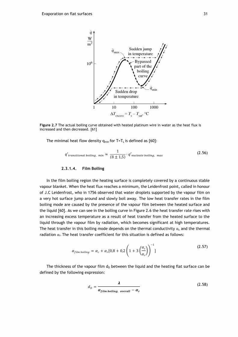
Evaporation on flat surfaces 31
Figure 2.7 The actual boiling curve obtained with heated platinum wire in water as the heat flux is increased and then decreased. [61]
The minimal heat flow density qmin for T=TL is defined as [60]:
𝑞′𝑡𝑟𝑎𝑛𝑠𝑖𝑡𝑖𝑜𝑛𝑎𝑙 𝑏𝑜𝑖𝑙𝑖𝑛𝑔, 𝑚𝑖𝑛 ≈ 1
(8 ± 1,5)∙ 𝑞′𝑛𝑢𝑐𝑙𝑒𝑎𝑡𝑒 𝑏𝑜𝑖𝑙𝑖𝑛𝑔, 𝑚𝑎𝑥 (2.56)
2.3.1.4. Film Boiling
In the film boiling region the heating surface is completely covered by a continuous stable
vapour blanket. When the heat flux reaches a minimum, the Leidenfrost point, called in honour
of J.C Leidenfrost, who in 1756 observed that water droplets supported by the vapour film on
a very hot surface jump around and slowly boil away. The low heat transfer rates in the film
boiling mode are caused by the presence of the vapour film between the heated surface and
the liquid [60]. As we can see in the boiling curve in Figure 2.6 the heat transfer rate rises with
an increasing excess temperature as a result of heat transfer from the heated surface to the
liquid through the vapour film by radiation, which becomes significant at high temperatures.
The heat transfer in this boiling mode depends on the thermal conductivity αc and the thermal
radiation αr. The heat transfer coefficient for this situation is defined as follows:
𝛼𝑓𝑖𝑙𝑚 𝑏𝑜𝑖𝑙𝑖𝑛𝑔 = 𝛼𝑐 + 𝛼𝑟[0,8 + 0,2 (1 + 3 (𝛼𝑐
𝛼𝑟
))
−1
] (2.57)
The thickness of the vapour film dD between the liquid and the heating flat surface can be
defined by the following expression:
𝑑𝐷 =𝞴
𝜶𝒇𝒊𝒍𝒎 𝒃𝒐𝒊𝒍𝒊𝒏𝒈, 𝒐𝒗𝒆𝒓𝒂𝒍𝒍 − 𝜶𝒓
(2.58)
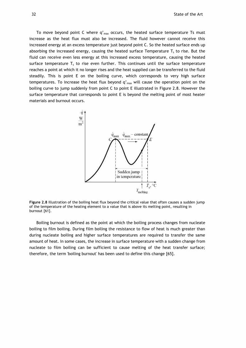
32 State of the Art
To move beyond point C where q’max occurs, the heated surface temperature Ts must
increase as the heat flux must also be increased. The fluid however cannot receive this
increased energy at an excess temperature just beyond point C. So the heated surface ends up
absorbing the increased energy, causing the heated surface Temperature Ts to rise. But the
fluid can receive even less energy at this increased excess temperature, causing the heated
surface temperature Ts to rise even further. This continues until the surface temperature
reaches a point at which it no longer rises and the heat supplied can be transferred to the fluid
steadily. This is point E on the boiling curve, which corresponds to very high surface
temperatures. To increase the heat flux beyond q’max will cause the operation point on the
boiling curve to jump suddenly from point C to point E illustrated in Figure 2.8. However the
surface temperature that corresponds to point E is beyond the melting point of most heater
materials and burnout occurs.
Figure 2.8 Illustration of the boiling heat flux beyond the critical value that often causes a sudden jump of the temperature of the heating element to a value that is above its melting point, resulting in burnout [61].
Boiling burnout is defined as the point at which the boiling process changes from nucleate
boiling to film boiling. During film boiling the resistance to flow of heat is much greater than
during nucleate boiling and higher surface temperatures are required to transfer the same
amount of heat. In some cases, the increase in surface temperature with a sudden change from
nucleate to film boiling can be sufficient to cause melting of the heat transfer surface;
therefore, the term 'boiling burnout' has been used to define this change [65].
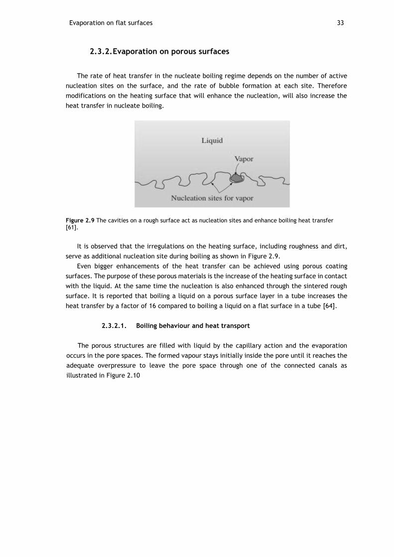
Evaporation on flat surfaces 33
2.3.2. Evaporation on porous surfaces
The rate of heat transfer in the nucleate boiling regime depends on the number of active
nucleation sites on the surface, and the rate of bubble formation at each site. Therefore
modifications on the heating surface that will enhance the nucleation, will also increase the
heat transfer in nucleate boiling.
Figure 2.9 The cavities on a rough surface act as nucleation sites and enhance boiling heat transfer [61].
It is observed that the irregulations on the heating surface, including roughness and dirt,
serve as additional nucleation site during boiling as shown in Figure 2.9.
Even bigger enhancements of the heat transfer can be achieved using porous coating
surfaces. The purpose of these porous materials is the increase of the heating surface in contact
with the liquid. At the same time the nucleation is also enhanced through the sintered rough
surface. It is reported that boiling a liquid on a porous surface layer in a tube increases the
heat transfer by a factor of 16 compared to boiling a liquid on a flat surface in a tube [64].
2.3.2.1. Boiling behaviour and heat transport
The porous structures are filled with liquid by the capillary action and the evaporation
occurs in the pore spaces. The formed vapour stays initially inside the pore until it reaches the
adequate overpressure to leave the pore space through one of the connected canals as
illustrated in Figure 2.10
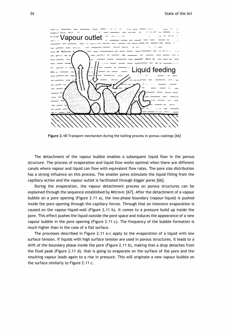
34 State of the Art
Figure 2.10 Transport mechanism during the boiling process in porous coatings [66]
The detachment of the vapour bubble enables a subsequent liquid flow in the porous
structure. The process of evaporation and liquid flow works optimal when there are different
canals where vapour and liquid can flow with equivalent flow rates. The pore size distribution
has a strong influence on this process. The smaller pores stimulate the liquid filling from the
capillary action and the vapour outlet is facilitated through bigger pores [66].
During the evaporation, the vapour detachment process on porous structures can be
explained through the sequence established by Mitrovic [67]. After the detachment of a vapour
bubble on a pore opening (Figure 2.11 a), the two-phase boundary (vapour-liquid) is pushed
inside the pore opening through the capillary forces. Through that an intensive evaporation is
caused on the vapour-liquid-wall (Figure 2.11 b). It comes to a pressure build up inside the
pore. This effect pushes the liquid outside the pore space and induces the appearance of a new
vapour bubble in the pore opening (Figure 2.11 c). The frequency of the bubble formation is
much higher than in the case of a flat surface.
The processes described in Figure 2.11 a-c apply to the evaporation of a liquid with low
surface tension. If liquids with high surface tension are used in porous structures, it leads to a
shift of the boundary phase inside the pore (Figure 2.11 b), making that a drop detaches from
the fluid peak (Figure 2.11 d), that is going to evaporate on the surface of the pore and the
resulting vapour leads again to a rise in pressure. This will originate a new vapour bubble on
the surface similarly to Figure 2.11 c.
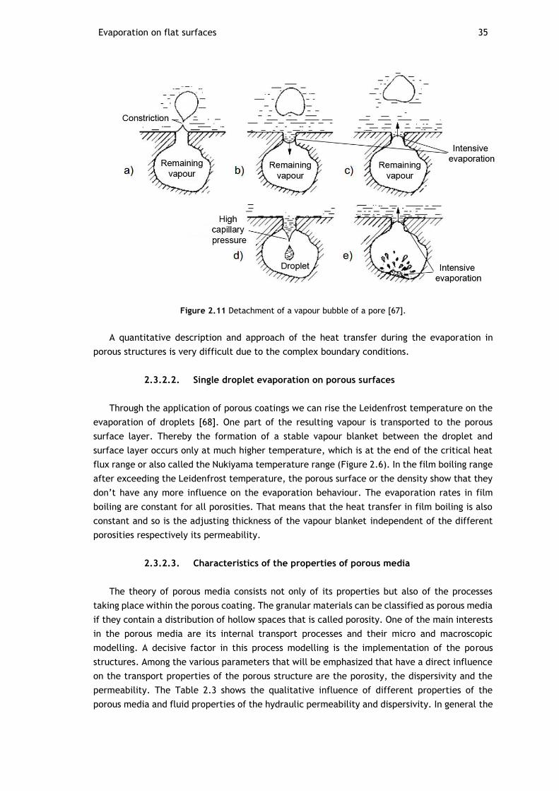
Evaporation on flat surfaces 35
Figure 2.11 Detachment of a vapour bubble of a pore [67].
A quantitative description and approach of the heat transfer during the evaporation in
porous structures is very difficult due to the complex boundary conditions.
2.3.2.2. Single droplet evaporation on porous surfaces
Through the application of porous coatings we can rise the Leidenfrost temperature on the
evaporation of droplets [68]. One part of the resulting vapour is transported to the porous
surface layer. Thereby the formation of a stable vapour blanket between the droplet and
surface layer occurs only at much higher temperature, which is at the end of the critical heat
flux range or also called the Nukiyama temperature range (Figure 2.6). In the film boiling range
after exceeding the Leidenfrost temperature, the porous surface or the density show that they
don’t have any more influence on the evaporation behaviour. The evaporation rates in film
boiling are constant for all porosities. That means that the heat transfer in film boiling is also
constant and so is the adjusting thickness of the vapour blanket independent of the different
porosities respectively its permeability.
2.3.2.3. Characteristics of the properties of porous media
The theory of porous media consists not only of its properties but also of the processes
taking place within the porous coating. The granular materials can be classified as porous media
if they contain a distribution of hollow spaces that is called porosity. One of the main interests
in the porous media are its internal transport processes and their micro and macroscopic
modelling. A decisive factor in this process modelling is the implementation of the porous
structures. Among the various parameters that will be emphasized that have a direct influence
on the transport properties of the porous structure are the porosity, the dispersivity and the
permeability. The Table 2.3 shows the qualitative influence of different properties of the
porous media and fluid properties of the hydraulic permeability and dispersivity. In general the
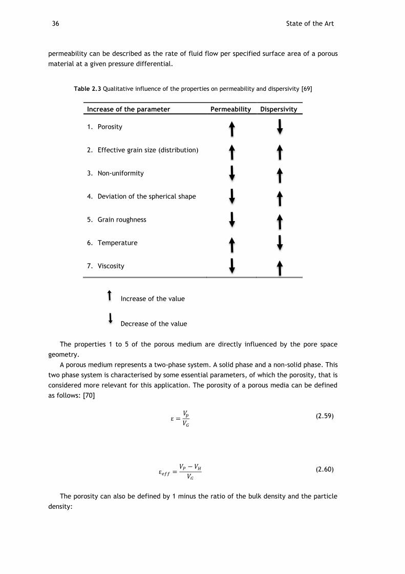
36 State of the Art
permeability can be described as the rate of fluid flow per specified surface area of a porous
material at a given pressure differential.
Table 2.3 Qualitative influence of the properties on permeability and dispersivity [69]
Increase of the parameter Permeability Dispersivity
1. Porosity
2. Effective grain size (distribution)
3. Non-uniformity
4. Deviation of the spherical shape
5. Grain roughness
6. Temperature
7. Viscosity
Increase of the value
Decrease of the value
The properties 1 to 5 of the porous medium are directly influenced by the pore space
geometry.
A porous medium represents a two-phase system. A solid phase and a non-solid phase. This
two phase system is characterised by some essential parameters, of which the porosity, that is
considered more relevant for this application. The porosity of a porous media can be defined
as follows: [70]
ε =𝑉𝑝
𝑉𝐺
(2.59)
ε𝑒𝑓𝑓 =𝑉𝑃 − 𝑉𝐻
𝑉𝐺
(2.60)
The porosity can also be defined by 1 minus the ratio of the bulk density and the particle
density:
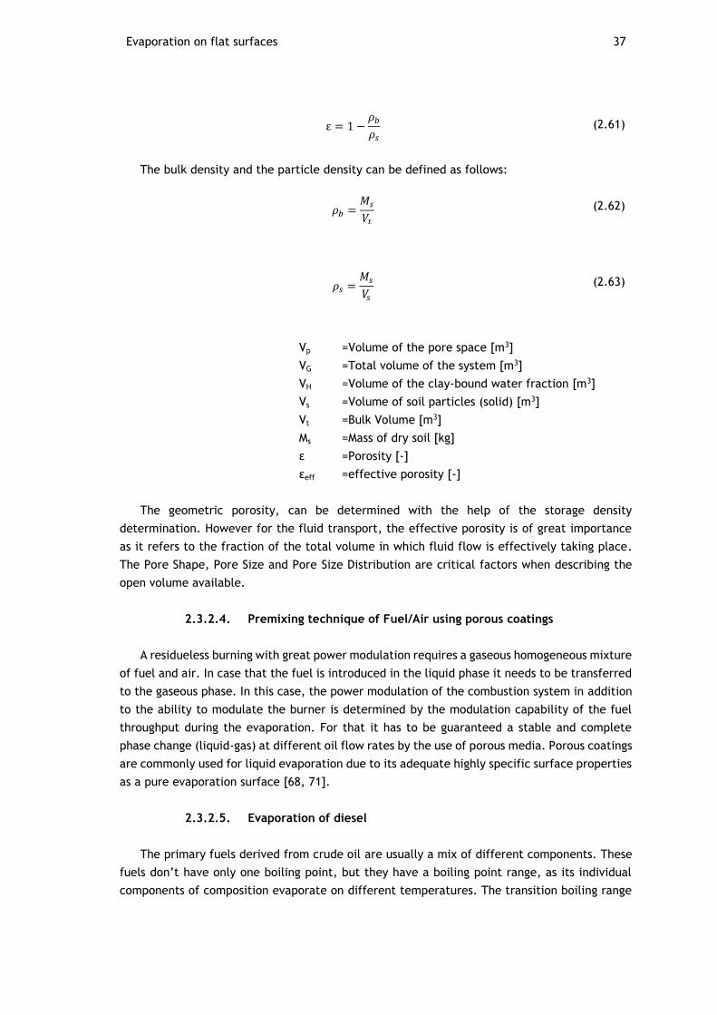
Evaporation on flat surfaces 37
ε = 1 −𝜌𝑏
𝜌𝑠
(2.61)
The bulk density and the particle density can be defined as follows:
𝜌𝑏 =𝑀𝑠
𝑉𝑡
(2.62)
𝜌𝑠 =𝑀𝑠
𝑉𝑠
(2.63)
Vp =Volume of the pore space [m3]
VG =Total volume of the system [m3]
VH =Volume of the clay-bound water fraction [m3]
Vs =Volume of soil particles (solid) [m3]
Vt =Bulk Volume [m3]
Ms =Mass of dry soil [kg]
ε =Porosity [-]
εeff =effective porosity [-]
The geometric porosity, can be determined with the help of the storage density
determination. However for the fluid transport, the effective porosity is of great importance
as it refers to the fraction of the total volume in which fluid flow is effectively taking place.
The Pore Shape, Pore Size and Pore Size Distribution are critical factors when describing the
open volume available.
2.3.2.4. Premixing technique of Fuel/Air using porous coatings
A residueless burning with great power modulation requires a gaseous homogeneous mixture
of fuel and air. In case that the fuel is introduced in the liquid phase it needs to be transferred
to the gaseous phase. In this case, the power modulation of the combustion system in addition
to the ability to modulate the burner is determined by the modulation capability of the fuel
throughput during the evaporation. For that it has to be guaranteed a stable and complete
phase change (liquid-gas) at different oil flow rates by the use of porous media. Porous coatings
are commonly used for liquid evaporation due to its adequate highly specific surface properties
as a pure evaporation surface [68, 71].
2.3.2.5. Evaporation of diesel
The primary fuels derived from crude oil are usually a mix of different components. These
fuels don’t have only one boiling point, but they have a boiling point range, as its individual
components of composition evaporate on different temperatures. The transition boiling range
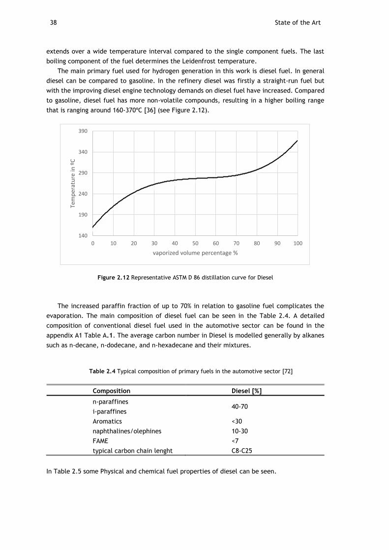
38 State of the Art
extends over a wide temperature interval compared to the single component fuels. The last
boiling component of the fuel determines the Leidenfrost temperature.
The main primary fuel used for hydrogen generation in this work is diesel fuel. In general
diesel can be compared to gasoline. In the refinery diesel was firstly a straight-run fuel but
with the improving diesel engine technology demands on diesel fuel have increased. Compared
to gasoline, diesel fuel has more non-volatile compounds, resulting in a higher boiling range
that is ranging around 160-370ºC [36] (see Figure 2.12).
Figure 2.12 Representative ASTM D 86 distillation curve for Diesel
The increased paraffin fraction of up to 70% in relation to gasoline fuel complicates the
evaporation. The main composition of diesel fuel can be seen in the Table 2.4. A detailed
composition of conventional diesel fuel used in the automotive sector can be found in the
appendix A1 Table A.1. The average carbon number in Diesel is modelled generally by alkanes
such as n-decane, n-dodecane, and n-hexadecane and their mixtures.
Table 2.4 Typical composition of primary fuels in the automotive sector [72]
Composition Diesel [%]
n-paraffines 40-70
i-paraffines
Aromatics <30
naphthalines/olephines 10-30
FAME <7
typical carbon chain lenght C8-C25
In Table 2.5 some Physical and chemical fuel properties of diesel can be seen.
140
190
240
290
340
390
0 10 20 30 40 50 60 70 80 90 100
Tem
per
atu
re in
ºC
vaporized volume percentage %
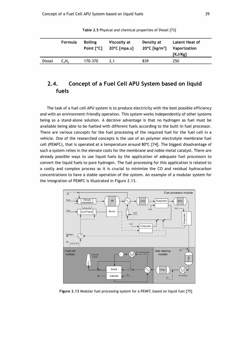
Concept of a Fuel Cell APU System based on liquid fuels 39
Table 2.5 Physical and chemical properties of Diesel [73]
Formula Boiling
Point [ºC]
Viscosity at
20ºC [mpa.s]
Density at
20ºC [kg/m3]
Latent Heat of
Vaporization
[KJ/Kg]
Diesel CxHy 170-370 3,1 839 250
2.4. Concept of a Fuel Cell APU System based on liquid
fuels
The task of a fuel cell APU system is to produce electricity with the best possible efficiency
and with an environment-friendly operation. This system works independently of other systems
being so a stand-alone solution. A decisive advantage is that no hydrogen as fuel must be
available being able to be fuelled with different fuels according to the built-in fuel processor.
There are various concepts for the fuel processing of the required fuel for the fuel cell in a
vehicle. One of the researched concepts is the use of an polymer electrolyte membrane fuel
cell (PEMFC), that is operated at a temperature around 80ºC [74]. The biggest disadvantage of
such a system relies in the elevate costs for the membrane and noble metal catalyst. There are
already possible ways to use liquid fuels by the application of adequate fuel processors to
convert the liquid fuels to pure hydrogen. The fuel processing for this application is related to
a costly and complex process as it is crucial to minimize the CO and residual hydrocarbon
concentrations to have a stable operation of the system. An example of a modular system for
the integration of PEMFC is illustrated in Figure 2.13.
Figure 2.13 Modular fuel processing system for a PEMFC based on liquid fuel [75]
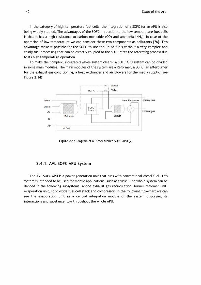
40 State of the Art
In the category of high temperature fuel cells, the integration of a SOFC for an APU is also
being widely studied. The advantages of the SOFC in relation to the low temperature fuel cells
is that it has a high resistance to carbon monoxide (CO) and ammonia (NH3). In case of the
operation of low temperature we can consider these two components as pollutants [76]. This
advantage make it possible for the SOFC to use the liquid fuels without a very complex and
costly fuel processing that can be directly coupled to the SOFC after the reforming process due
to its high temperature operation.
To make the complex, integrated whole system clearer a SOFC APU system can be divided
in some main modules. The main modules of the system are a Reformer, a SOFC, an afterburner
for the exhaust gas conditioning, a heat exchanger and air blowers for the media supply. (see
Figure 2.14)
Figure 2.14 Diagram of a Diesel fuelled SOFC-APU [7]
2.4.1. AVL SOFC APU System
The AVL SOFC APU is a power generation unit that runs with conventional diesel fuel. This
system is intended to be used for mobile applications, such as trucks. The whole system can be
divided in the following subsystems; anode exhaust gas recirculation, burner-reformer unit,
evaporation unit, solid oxide fuel cell stack and compressor. In the following flowchart we can
see the evaporation unit as a central integration module of the system displaying its
interactions and substance flow throughout the whole APU.
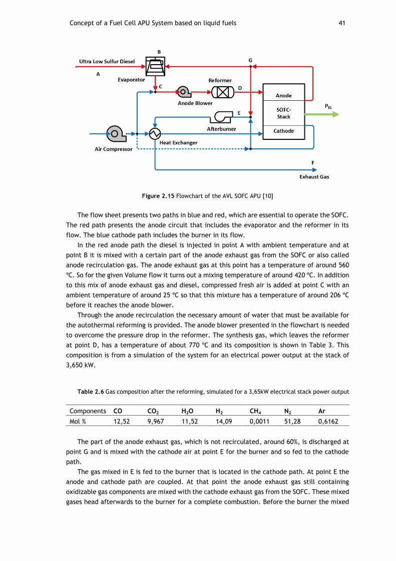
Concept of a Fuel Cell APU System based on liquid fuels 41
Figure 2.15 Flowchart of the AVL SOFC APU [10]
The flow sheet presents two paths in blue and red, which are essential to operate the SOFC.
The red path presents the anode circuit that includes the evaporator and the reformer in its
flow. The blue cathode path includes the burner in its flow.
In the red anode path the diesel is injected in point A with ambient temperature and at
point B it is mixed with a certain part of the anode exhaust gas from the SOFC or also called
anode recirculation gas. The anode exhaust gas at this point has a temperature of around 560
ºC. So for the given Volume flow it turns out a mixing temperature of around 420 ºC. In addition
to this mix of anode exhaust gas and diesel, compressed fresh air is added at point C with an
ambient temperature of around 25 ºC so that this mixture has a temperature of around 206 ºC
before it reaches the anode blower.
Through the anode recirculation the necessary amount of water that must be available for
the autothermal reforming is provided. The anode blower presented in the flowchart is needed
to overcome the pressure drop in the reformer. The synthesis gas, which leaves the reformer
at point D, has a temperature of about 770 ºC and its composition is shown in Table 3. This
composition is from a simulation of the system for an electrical power output at the stack of
3,650 kW.
Table 2.6 Gas composition after the reforming, simulated for a 3,65kW electrical stack power output
Components CO CO2 H2O H2 CH4 N2 Ar
Mol % 12,52 9,967 11,52 14,09 0,0011 51,28 0,6162
The part of the anode exhaust gas, which is not recirculated, around 60%, is discharged at
point G and is mixed with the cathode air at point E for the burner and so fed to the cathode
path.
The gas mixed in E is fed to the burner that is located in the cathode path. At point E the
anode and cathode path are coupled. At that point the anode exhaust gas still containing
oxidizable gas components are mixed with the cathode exhaust gas from the SOFC. These mixed
gases head afterwards to the burner for a complete combustion. Before the burner the mixed
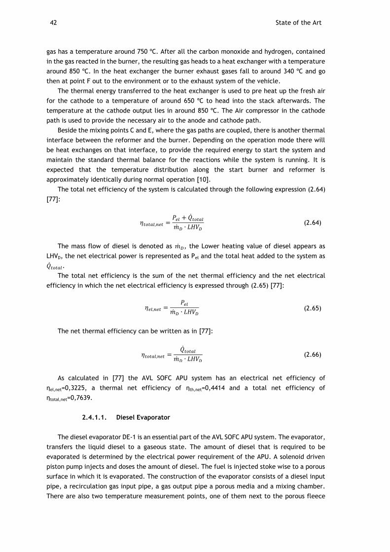
42 State of the Art
gas has a temperature around 750 ºC. After all the carbon monoxide and hydrogen, contained
in the gas reacted in the burner, the resulting gas heads to a heat exchanger with a temperature
around 850 ºC. In the heat exchanger the burner exhaust gases fall to around 340 ºC and go
then at point F out to the environment or to the exhaust system of the vehicle.
The thermal energy transferred to the heat exchanger is used to pre heat up the fresh air
for the cathode to a temperature of around 650 ºC to head into the stack afterwards. The
temperature at the cathode output lies in around 850 ºC. The Air compressor in the cathode
path is used to provide the necessary air to the anode and cathode path.
Beside the mixing points C and E, where the gas paths are coupled, there is another thermal
interface between the reformer and the burner. Depending on the operation mode there will
be heat exchanges on that interface, to provide the required energy to start the system and
maintain the standard thermal balance for the reactions while the system is running. It is
expected that the temperature distribution along the start burner and reformer is
approximately identically during normal operation [10].
The total net efficiency of the system is calculated through the following expression (2.64)
[77]:
𝜂𝑡𝑜𝑡𝑎𝑙,𝑛𝑒𝑡 =𝑃𝑒𝑙 + �̇�𝑡𝑜𝑡𝑎𝑙
�̇�𝐷 ∙ 𝐿𝐻𝑉𝐷
(2.64)
The mass flow of diesel is denoted as �̇�𝐷, the Lower heating value of diesel appears as
LHVD, the net electrical power is represented as Pel and the total heat added to the system as
�̇�𝑡𝑜𝑡𝑎𝑙.
The total net efficiency is the sum of the net thermal efficiency and the net electrical
efficiency in which the net electrical efficiency is expressed through (2.65) [77]:
𝜂𝑒𝑙,𝑛𝑒𝑡 =𝑃𝑒𝑙
�̇�𝐷 ∙ 𝐿𝐻𝑉𝐷
(2.65)
The net thermal efficiency can be written as in [77]:
𝜂𝑡𝑜𝑡𝑎𝑙,𝑛𝑒𝑡 =�̇�𝑡𝑜𝑡𝑎𝑙
�̇�𝐷 ∙ 𝐿𝐻𝑉𝐷
(2.66)
As calculated in [77] the AVL SOFC APU system has an electrical net efficiency of
ηel,net=0,3225, a thermal net efficiency of ηth,net=0,4414 and a total net efficiency of
ηtotal,net=0,7639.
2.4.1.1. Diesel Evaporator
The diesel evaporator DE-1 is an essential part of the AVL SOFC APU system. The evaporator,
transfers the liquid diesel to a gaseous state. The amount of diesel that is required to be
evaporated is determined by the electrical power requirement of the APU. A solenoid driven
piston pump injects and doses the amount of diesel. The fuel is injected stoke wise to a porous
surface in which it is evaporated. The construction of the evaporator consists of a diesel input
pipe, a recirculation gas input pipe, a gas output pipe a porous media and a mixing chamber.
There are also two temperature measurement points, one of them next to the porous fleece
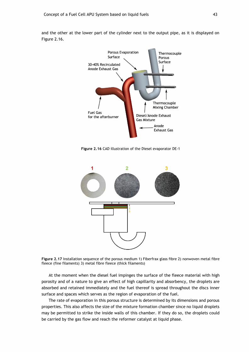
Concept of a Fuel Cell APU System based on liquid fuels 43
and the other at the lower part of the cylinder next to the output pipe, as it is displayed on
Figure 2.16.
Figure 2.16 CAD illustration of the Diesel evaporator DE-1
Figure 2.17 Installation sequence of the porous medium 1) Fiberfrax glass fibre 2) nonwoven metal fibre fleece (fine filaments) 3) metal fibre fleece (thick filaments)
At the moment when the diesel fuel impinges the surface of the fleece material with high
porosity and of a nature to give an effect of high capillarity and absorbency, the droplets are
absorbed and retained immediately and the fuel thereof is spread throughout the discs inner
surface and spaces which serves as the region of evaporation of the fuel.
The rate of evaporation in this porous structure is determined by its dimensions and porous
properties. This also affects the size of the mixture formation chamber since no liquid droplets
may be permitted to strike the inside walls of this chamber. If they do so, the droplets could
be carried by the gas flow and reach the reformer catalyst at liquid phase.
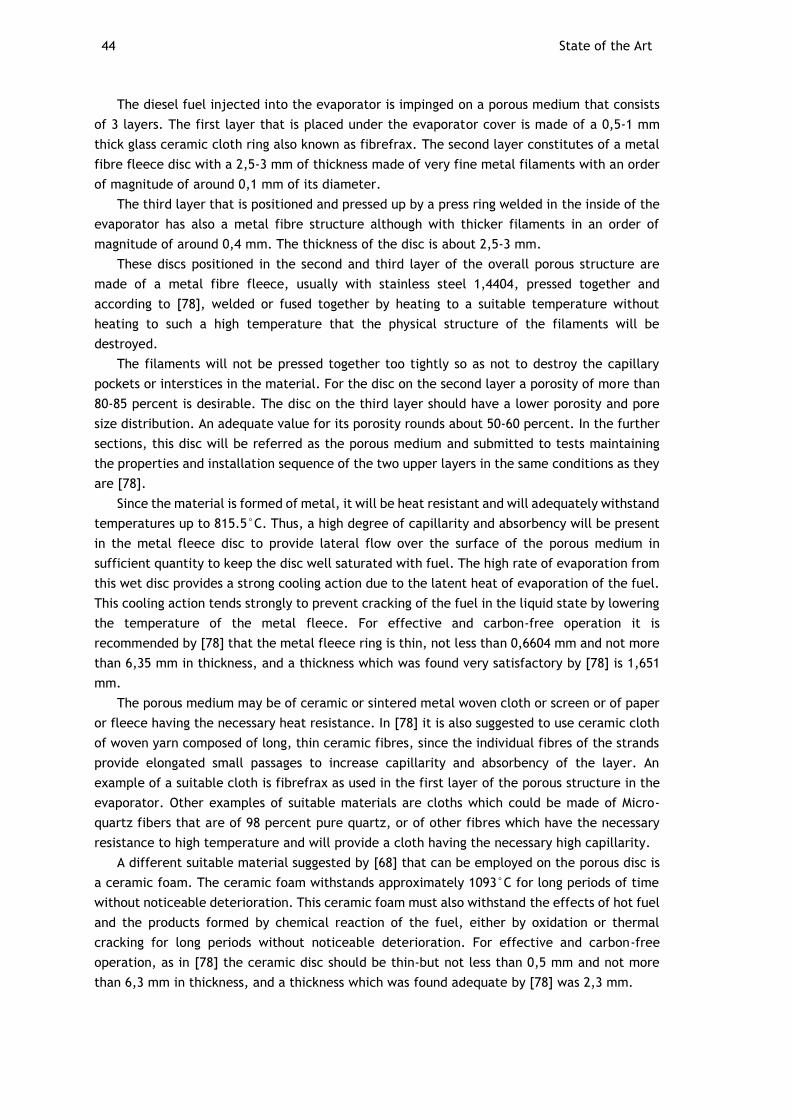
44 State of the Art
The diesel fuel injected into the evaporator is impinged on a porous medium that consists
of 3 layers. The first layer that is placed under the evaporator cover is made of a 0,5-1 mm
thick glass ceramic cloth ring also known as fibrefrax. The second layer constitutes of a metal
fibre fleece disc with a 2,5-3 mm of thickness made of very fine metal filaments with an order
of magnitude of around 0,1 mm of its diameter.
The third layer that is positioned and pressed up by a press ring welded in the inside of the
evaporator has also a metal fibre structure although with thicker filaments in an order of
magnitude of around 0,4 mm. The thickness of the disc is about 2,5-3 mm.
These discs positioned in the second and third layer of the overall porous structure are
made of a metal fibre fleece, usually with stainless steel 1,4404, pressed together and
according to [78], welded or fused together by heating to a suitable temperature without
heating to such a high temperature that the physical structure of the filaments will be
destroyed.
The filaments will not be pressed together too tightly so as not to destroy the capillary
pockets or interstices in the material. For the disc on the second layer a porosity of more than
80-85 percent is desirable. The disc on the third layer should have a lower porosity and pore
size distribution. An adequate value for its porosity rounds about 50-60 percent. In the further
sections, this disc will be referred as the porous medium and submitted to tests maintaining
the properties and installation sequence of the two upper layers in the same conditions as they
are [78].
Since the material is formed of metal, it will be heat resistant and will adequately withstand
temperatures up to 815.5°C. Thus, a high degree of capillarity and absorbency will be present
in the metal fleece disc to provide lateral flow over the surface of the porous medium in
sufficient quantity to keep the disc well saturated with fuel. The high rate of evaporation from
this wet disc provides a strong cooling action due to the latent heat of evaporation of the fuel.
This cooling action tends strongly to prevent cracking of the fuel in the liquid state by lowering
the temperature of the metal fleece. For effective and carbon-free operation it is
recommended by [78] that the metal fleece ring is thin, not less than 0,6604 mm and not more
than 6,35 mm in thickness, and a thickness which was found very satisfactory by [78] is 1,651
mm.
The porous medium may be of ceramic or sintered metal woven cloth or screen or of paper
or fleece having the necessary heat resistance. In [78] it is also suggested to use ceramic cloth
of woven yarn composed of long, thin ceramic fibres, since the individual fibres of the strands
provide elongated small passages to increase capillarity and absorbency of the layer. An
example of a suitable cloth is fibrefrax as used in the first layer of the porous structure in the
evaporator. Other examples of suitable materials are cloths which could be made of Micro-
quartz fibers that are of 98 percent pure quartz, or of other fibres which have the necessary
resistance to high temperature and will provide a cloth having the necessary high capillarity.
A different suitable material suggested by [68] that can be employed on the porous disc is
a ceramic foam. The ceramic foam withstands approximately 1093°C for long periods of time
without noticeable deterioration. This ceramic foam must also withstand the effects of hot fuel
and the products formed by chemical reaction of the fuel, either by oxidation or thermal
cracking for long periods without noticeable deterioration. For effective and carbon-free
operation, as in [78] the ceramic disc should be thin-but not less than 0,5 mm and not more
than 6,3 mm in thickness, and a thickness which was found adequate by [78] was 2,3 mm.
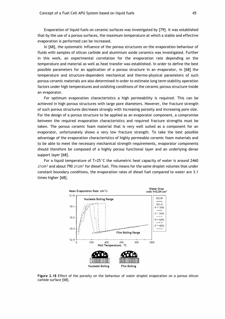
Concept of a Fuel Cell APU System based on liquid fuels 45
Evaporation of liquid fuels on ceramic surfaces was investigated by [79]. It was established
that by the use of a porous surfaces, the maximum temperature at which a stable and effective
evaporation is performed can be increased.
In [68], the systematic influence of the porous structures on the evaporation behaviour of
fluids with samples of silicon carbide and aluminium oxide ceramics was investigated. Further
in this work, an experimental correlation for the evaporation rate depending on the
temperature and material as well as heat transfer was established. In order to define the best
possible parameters for an application of a porous structure in an evaporator, in [68] the
temperature and structure-dependent mechanical and thermo-physical parameters of such
porous ceramic materials are also determined in order to estimate long term stability operation
factors under high temperatures and oxidizing conditions of the ceramic porous structure inside
an evaporator.
For optimum evaporation characteristics a high permeability is required. This can be
achieved in high porous structures with large pore diameters. However, the fracture strength
of such porous structures decreases strongly with increasing porosity and increasing pore size.
For the design of a porous structure to be applied as an evaporator component, a compromise
between the required evaporation characteristics and required fracture strengths must be
taken. The porous ceramic foam material that is very well suited as a component for an
evaporator, unfortunately shows a very low fracture strength. To take the best possible
advantage of the evaporation characteristics of highly permeable ceramic foam materials and
to be able to meet the necessary mechanical strength requirements, evaporator components
should therefore be composed of a highly porous functional layer and an underlying dense
support layer [68].
For a liquid temperature of T=25°C the volumetric heat capacity of water is around 2460
J/cm³ and about 790 J/cm³ for diesel fuel. This means for the same droplet volumes that under
constant boundary conditions, the evaporation rates of diesel fuel compared to water are 3.1
times higher [68].
Figure 2.18 Effect of the porosity on the behaviour of water droplet evaporation on a porous silicon carbide surface [68].
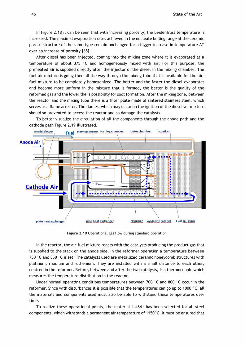
46 State of the Art
In Figure 2.18 it can be seen that with increasing porosity, the Leidenfrost temperature is
increased. The maximal evaporation rates achieved in the nucleate boiling range at the ceramic
porous structure of the same type remain unchanged for a bigger increase in temperature ΔT
over an increase of porosity [68].
After diesel has been injected, coming into the mixing zone where it is evaporated at a
temperature of about 375 °C and homogeneously mixed with air. For this purpose, the
preheated air is supplied directly after the injector of the diesel in the mixing chamber. The
fuel-air mixture is going then all the way through the mixing tube that is available for the air-
fuel mixture to be completely homogenized. The better and the faster the diesel evaporates
and become more uniform in the mixture that is formed, the better is the quality of the
reformed gas and the lower the is possibility for soot formation. After the mixing zone, between
the reactor and the mixing tube there is a filter plate made of sintered stainless steel, which
serves as a flame arrester. The flames, which may occur on the ignition of the diesel-air mixture
should so prevented to access the reactor and so damage the catalysts.
To better visualize the circulation of all the components through the anode path and the
cathode path Figure 2.19 illustrated.
Figure 2.19 Operational gas flow during standard operation
In the reactor, the air-fuel mixture reacts with the catalysts producing the product gas that
is supplied to the stack on the anode side. In the reformer operation a temperature between
750 °C and 850 °C is set. The catalysts used are metallized ceramic honeycomb structures with
platinum, rhodium and ruthenium. They are installed with a small distance to each other,
centred in the reformer. Before, between and after the two catalysts, is a thermocouple which
measures the temperature distribution in the reactor.
Under normal operating conditions temperatures between 700 °C and 800 °C occur in the
reformer. Since with disturbances it is possible that the temperatures can go up to 1000 °C, all
the materials and components used must also be able to withstand these temperatures over
time.
To realize these operational points, the material 1.4841 has been selected for all steel
components, which withstands a permanent air temperature of 1150°C. It must be ensured that
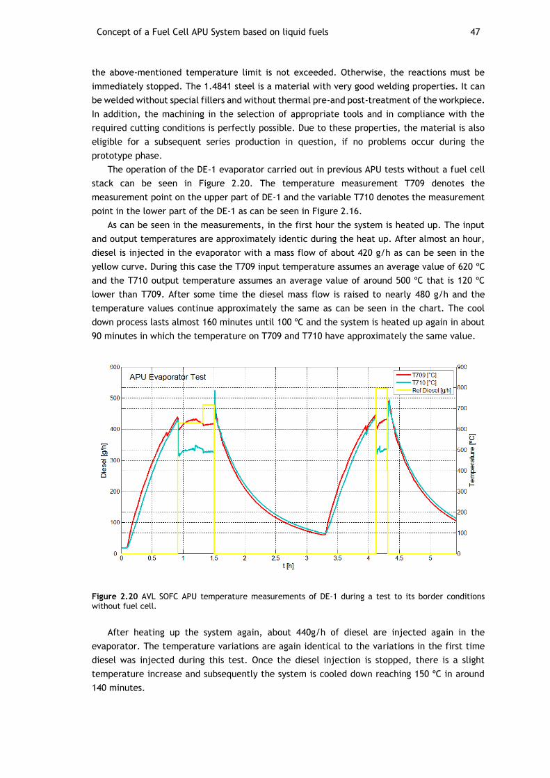
Concept of a Fuel Cell APU System based on liquid fuels 47
the above-mentioned temperature limit is not exceeded. Otherwise, the reactions must be
immediately stopped. The 1.4841 steel is a material with very good welding properties. It can
be welded without special fillers and without thermal pre-and post-treatment of the workpiece.
In addition, the machining in the selection of appropriate tools and in compliance with the
required cutting conditions is perfectly possible. Due to these properties, the material is also
eligible for a subsequent series production in question, if no problems occur during the
prototype phase.
The operation of the DE-1 evaporator carried out in previous APU tests without a fuel cell
stack can be seen in Figure 2.20. The temperature measurement T709 denotes the
measurement point on the upper part of DE-1 and the variable T710 denotes the measurement
point in the lower part of the DE-1 as can be seen in Figure 2.16.
As can be seen in the measurements, in the first hour the system is heated up. The input
and output temperatures are approximately identic during the heat up. After almost an hour,
diesel is injected in the evaporator with a mass flow of about 420 g/h as can be seen in the
yellow curve. During this case the T709 input temperature assumes an average value of 620 ºC
and the T710 output temperature assumes an average value of around 500 ºC that is 120 ºC
lower than T709. After some time the diesel mass flow is raised to nearly 480 g/h and the
temperature values continue approximately the same as can be seen in the chart. The cool
down process lasts almost 160 minutes until 100 ºC and the system is heated up again in about
90 minutes in which the temperature on T709 and T710 have approximately the same value.
Figure 2.20 AVL SOFC APU temperature measurements of DE-1 during a test to its border conditions without fuel cell.
After heating up the system again, about 440g/h of diesel are injected again in the
evaporator. The temperature variations are again identical to the variations in the first time
diesel was injected during this test. Once the diesel injection is stopped, there is a slight
temperature increase and subsequently the system is cooled down reaching 150 ºC in around
140 minutes.

48 State of the Art
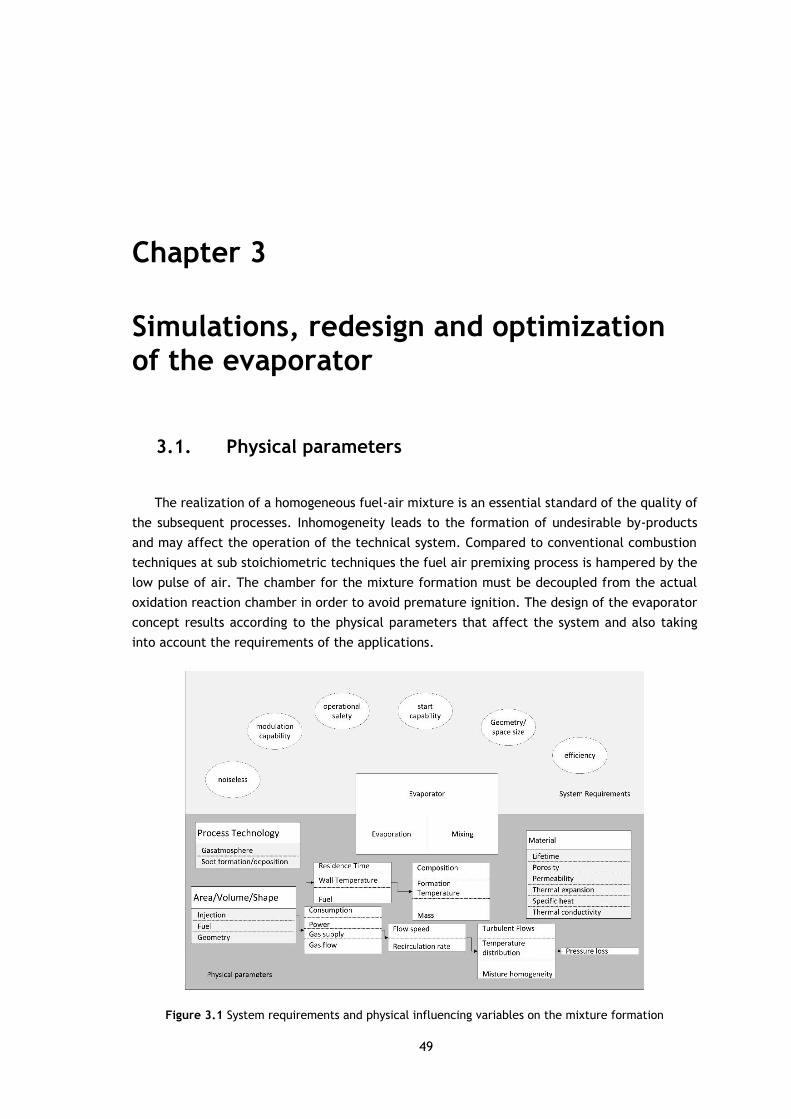
49
Chapter 3
Simulations, redesign and optimization of the evaporator
3.1. Physical parameters
The realization of a homogeneous fuel-air mixture is an essential standard of the quality of
the subsequent processes. Inhomogeneity leads to the formation of undesirable by-products
and may affect the operation of the technical system. Compared to conventional combustion
techniques at sub stoichiometric techniques the fuel air premixing process is hampered by the
low pulse of air. The chamber for the mixture formation must be decoupled from the actual
oxidation reaction chamber in order to avoid premature ignition. The design of the evaporator
concept results according to the physical parameters that affect the system and also taking
into account the requirements of the applications.
Figure 3.1 System requirements and physical influencing variables on the mixture formation
50 Simulations, redesign and optimization of the evaporator
The mixture formation can be divided into two separate parallel running processes, the
actual vaporization of the fuel and the subsequent mixing with the anode exhaust gas. The
evaporation is in the physical sense the passage of a liquid substance in the gaseous state
through evaporation and boiling (see 2.3). The evaporation enthalpy describes the amount of
heat required to convert the liquid into vapour at the same temperature, at unaltered pressure.
The main physical influence factors on the evaporation are the temperature, total pressure,
and the proportions of the starting materials, the time and the droplet size distribution and the
flow type.
Boiling is the transition of a liquid into the gaseous state at a given temperature, its boiling
point. The boiling temperature increases with increasing pressure. In general, the evaporation
temperature of a liquid substance is equal to its boiling temperature at atmospheric pressure.
As diesel is a mixture of several components it can’t be specified a concrete saturation
temperature, instead it will have a boiling range (see section 2.3.2.5).
The quality of the mixture formation depends not only on the pressure and the temperature
inside the evaporator but on more three main parameters, the droplet size distribution of the
fuel spray, the time and the gas flow in the mixture formation chamber. In the investigated
evaporator DE-1 the fuel is supplied through a porous medium. In that medium the volume
decrease of the droplets injected on it, with a given frequency and the distributions of the fuel
on that medium depends mainly on the porosity and pore size distribution of that medium. The
subject about porous materials will not be analysed in detail although there are going to be
made some tests with different materials and porosities to analyse the effect of it on the
evaporation and the soot formation.
Increased turbulence of the gas flow supports the mixture formation, it is improved by the
heat and material exchange between the fuel spray and the surrounding fluid.
3.2. System requirements
The start ability of the evaporator must be always ensured. For the use of a diesel reformer
in mobile applications a start capability down to minus forty degrees Celsius is projected. The
use of electrical energy to the heating system is not useful because of the high heat capacity.
The heat required for the start of the system is obtained by a start burner that is installed in
an annular ring chamber. This heat heats up the system by convective heat transfer. After an
estimated time of 30 minutes the system reaches the required operation temperature and on
the start of operation the fuel feed to the start burner is stopped. At that point the evaporation
chamber has sufficient heat to prepare a homogenous mixture.
The reliability (operational safety) of an evaporator is accomplished when a homogeneous
mixture formation occurs in all operating points. An incomplete evaporation of the fuel or re-
condensation on cold components can lead to precipitation of fuel or carbon deposits in the
mixture formation chamber. The required temperature level as well as the residence time
favour a self-ignition of the mixture. The resulting combustion temperatures can cause damage
to the components in the evaporator and also to components in subsequent process steps.
The stationary operation and the initial phase of the system must be energy efficient. The
use of electrical energy for pumps, compressors and electric heating is kept to a minimum. The
Evaporator experimental fuel processing simulation 51
geometrical requirements of the evaporator results from the overall concept and should be
adjusted accordingly. Especially in the mobile application the space of the system is very
limited.
Depending on the application, the acoustic behaviour is of great importance. Although a
high turbulence of the air flow improves the heat and mass transfer in the mixture formation,
but the consequence of it is that these parameters increase the noise emissions and also
pressure losses. Low complexity by using standard components and a simple controllability are
crucial for the cost of the evaporator.
3.3. Evaporator experimental fuel processing simulation
To plan and to actively pursue the further presented and described experiments a 1D
Simulation with Matlab/Simulink has been carried out. This is also based on the experiences
that have been made in the development of the reformer [80]. For simulation purposes
hexadecane (C16H34) is used as the modelling component to approximate the results to diesel.
To create the simulation model that reflects the experimental setup, an internal model
library developed in AVL for Matlab/Simulink [77] is available, which includes all necessary
components such as the evaporator, the reformer and a catalytic burner. Through that, the
vaporization enthalpy of diesel fuel and the mixture formation of gases can be calculated. As
input variables for all calculations, compositions can be given as input for the individual
components. In the model parts, such as the burner, other boundary conditions such as heat
radiation and burner surface can be entered. As output from the simulation results a
calculation, which indicates the conversion of the products of the chemical reactions
excessively close to reality. Information on flow rates and temperatures of the product gases
can also be extracted as results of the model.
In the concrete case, the simulation model that is shown in Figure 3.2 has been created to
analyse data for the further experimental setup. The following data must be entered in the
pre-processing.
Recirculated anode gas composition and temperature.
The diesel amount that is injected in the evaporator according to a desired
electrical load point of the fuel cell.
The amount and temperature of air added before the reformer (anode air).
The amount and temperature of air added before the catalytic burner (cathode
air).
According to the desired operation conditions the system can be calibrated to operate in a
more efficient way. The parameters that can be analysed as output are:
The evaporator, reformer and burner output temperature, pressure and mass flow.
The reacted and yielded components in the evaporator, reformer and burner
output.
The evaporation enthalpy difference at the evaporator output.
The reaction enthalpy, efficiency of the fuel reforming, probability to carbon
formation, steam to carbon ratio, oxygen to carbon ratio, pressure loss, thermal
output power and oxygen to diesel ratio (𝞴) at the output of the reformer.
The air to fuel ratio, pressure loss and heat of reaction at the burner output.
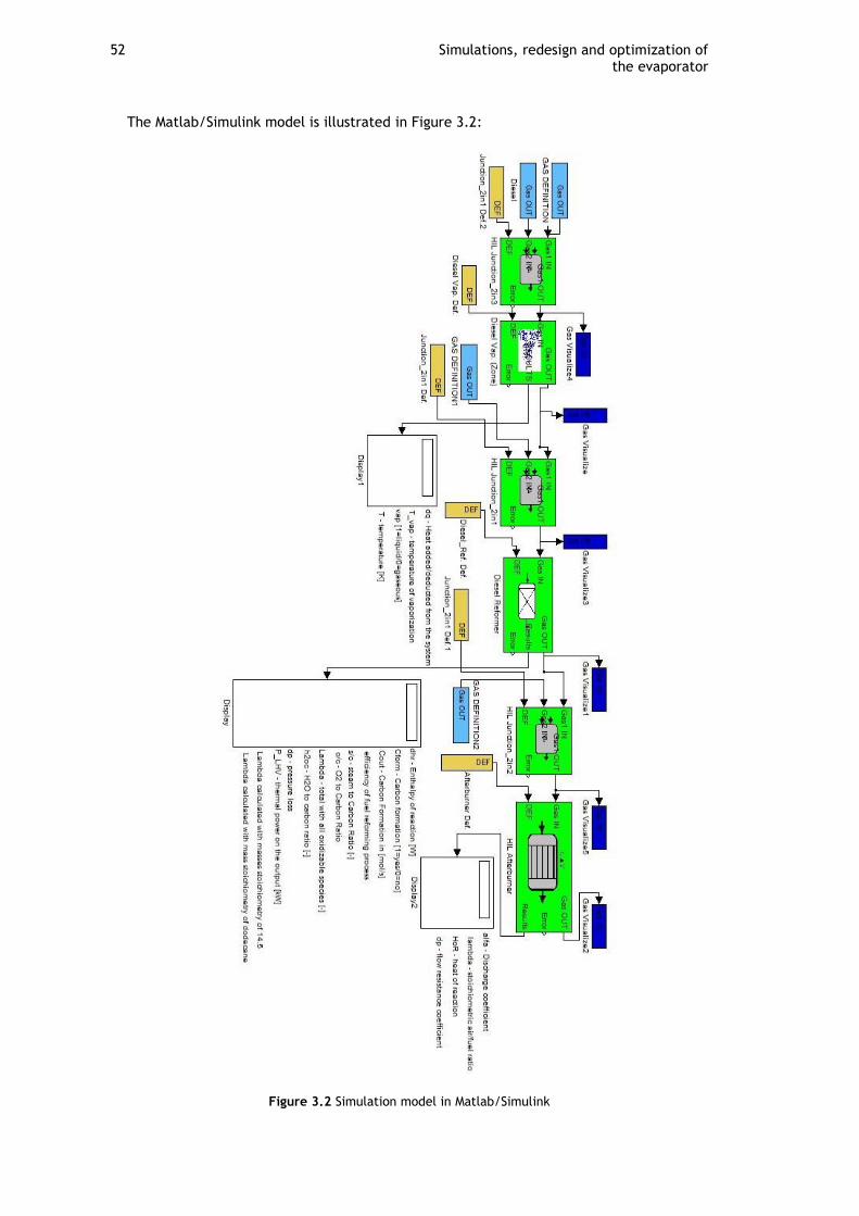
52 Simulations, redesign and optimization of the evaporator
The Matlab/Simulink model is illustrated in Figure 3.2:
Figure 3.2 Simulation model in Matlab/Simulink
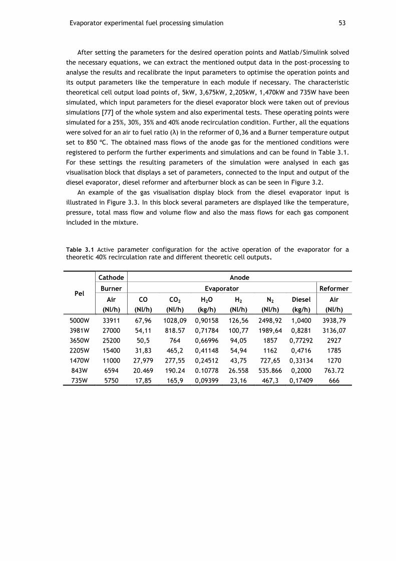
Evaporator experimental fuel processing simulation 53
After setting the parameters for the desired operation points and Matlab/Simulink solved
the necessary equations, we can extract the mentioned output data in the post-processing to
analyse the results and recalibrate the input parameters to optimise the operation points and
its output parameters like the temperature in each module if necessary. The characteristic
theoretical cell output load points of, 5kW, 3,675kW, 2,205kW, 1,470kW and 735W have been
simulated, which input parameters for the diesel evaporator block were taken out of previous
simulations [77] of the whole system and also experimental tests. These operating points were
simulated for a 25%, 30%, 35% and 40% anode recirculation condition. Further, all the equations
were solved for an air to fuel ratio (λ) in the reformer of 0,36 and a Burner temperature output
set to 850 ºC. The obtained mass flows of the anode gas for the mentioned conditions were
registered to perform the further experiments and simulations and can be found in Table 3.1.
For these settings the resulting parameters of the simulation were analysed in each gas
visualisation block that displays a set of parameters, connected to the input and output of the
diesel evaporator, diesel reformer and afterburner block as can be seen in Figure 3.2.
An example of the gas visualisation display block from the diesel evaporator input is
illustrated in Figure 3.3. In this block several parameters are displayed like the temperature,
pressure, total mass flow and volume flow and also the mass flows for each gas component
included in the mixture.
Table 3.1 Active parameter configuration for the active operation of the evaporator for a theoretic 40% recirculation rate and different theoretic cell outputs.
Pel
Cathode Anode
Burner Evaporator Reformer
Air
(Nl/h)
CO
(Nl/h)
CO2
(Nl/h)
H2O
(kg/h)
H2
(Nl/h)
N2
(Nl/h)
Diesel
(kg/h)
Air
(Nl/h)
5000W 33911 67,96 1028,09 0,90158 126,56 2498,92 1,0400 3938,79
3981W 27000 54,11 818.57 0,71784 100,77 1989,64 0,8281 3136,07
3650W 25200 50,5 764 0,66996 94,05 1857 0,77292 2927
2205W 15400 31,83 465,2 0,41148 54,94 1162 0,4716 1785
1470W 11000 27,979 277,55 0,24512 43,75 727,65 0,33134 1270
843W 6594 20.469 190.24 0.10778 26.558 535.866 0,2000 763.72
735W 5750 17,85 165,9 0,09399 23,16 467,3 0,17409 666
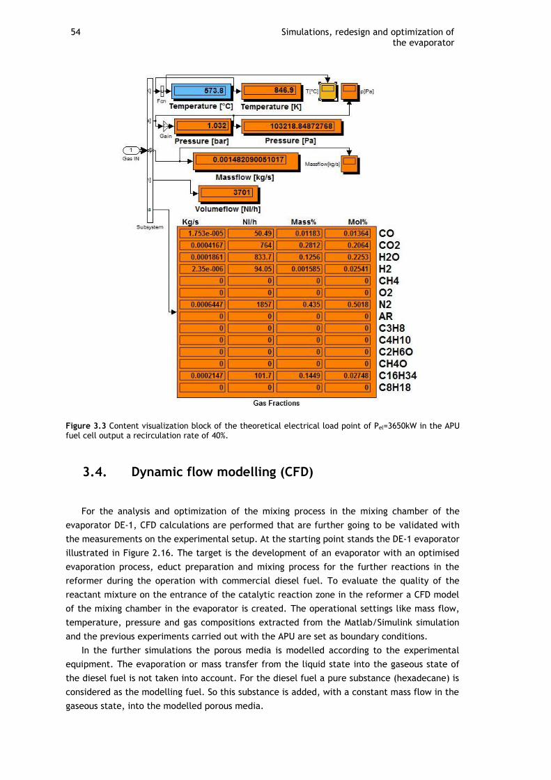
54 Simulations, redesign and optimization of the evaporator
Figure 3.3 Content visualization block of the theoretical electrical load point of Pel=3650kW in the APU fuel cell output a recirculation rate of 40%.
3.4. Dynamic flow modelling (CFD)
For the analysis and optimization of the mixing process in the mixing chamber of the
evaporator DE-1, CFD calculations are performed that are further going to be validated with
the measurements on the experimental setup. At the starting point stands the DE-1 evaporator
illustrated in Figure 2.16. The target is the development of an evaporator with an optimised
evaporation process, educt preparation and mixing process for the further reactions in the
reformer during the operation with commercial diesel fuel. To evaluate the quality of the
reactant mixture on the entrance of the catalytic reaction zone in the reformer a CFD model
of the mixing chamber in the evaporator is created. The operational settings like mass flow,
temperature, pressure and gas compositions extracted from the Matlab/Simulink simulation
and the previous experiments carried out with the APU are set as boundary conditions.
In the further simulations the porous media is modelled according to the experimental
equipment. The evaporation or mass transfer from the liquid state into the gaseous state of
the diesel fuel is not taken into account. For the diesel fuel a pure substance (hexadecane) is
considered as the modelling fuel. So this substance is added, with a constant mass flow in the
gaseous state, into the modelled porous media.
Dynamic flow modelling (CFD) 55
In addition to determine the mixture quality at the entrance of the reformer catalyst, the
target of the fluid dynamic modelling of the mixing chamber of the evaporator is to describe
the flow pattern along the mixing chamber and to identify possible not mixed zones. Through
the analysis of the flow pattern possible pressure losses can be identified to improve the flow
as the efficiency of the APU lowers with higher pressure losses. This means that the compressors
and blowers need more electrical energy from the electrical power output of the SOFC for their
operation.
These analysis allow the detection of weak points of the respective construction. Through
this knowledge changes can be performed on the mixing chamber geometry of the DE-1
evaporator that lead to a better mixing process.
The achieved results will be compared with the experimental diagnosis. From this further
comparison can be detected which thermodynamic conditions can lead to process related
difficulties such as mainly carbon formation. It must be emphasized that CFD modelling is just
a helping tool and an approximation of the real solution. It helps interpreting the theoretical
and practical results and it cannot take all the physical and chemical processes into account.
The implementation of this part of the project was divided into three main steps: the pre-
processing and the configuration of the simulation, the solving of the equations by numerical
methods and the post-processing and visualisation of the results.
3.4.1. Pre-processing
In this step all the input of a flow problem is set up in AVL Fire through its operator-friendly
interface that in a subsequent internal configurations sets up the data in a suitable form for
the use in its solver. The elaboration of the pre-processing activities was divided into the
following steps:
Design of CAD geometries according to the dimensions and implementation in the
APU.
Definition of the region of interest of every redesigned geometry in the
computational domain.
Grid generation and building a mesh, subdividing the domain into a number of
smaller non overlapping sub-domains like a grid of cells.
Setting and selection of the physical process that is to be modelled
Appropriate dimension of the boundary conditions.
3.4.1.1. The Geometry
The DE-1 evaporator is a full scale CAD-model designed in PTC Creo Elements Pro 5.0 as
part of the whole APU system model as we can see in Figure 2.16. The implementation of the
DE-1 in the APU can be seen in the following CAD illustration.
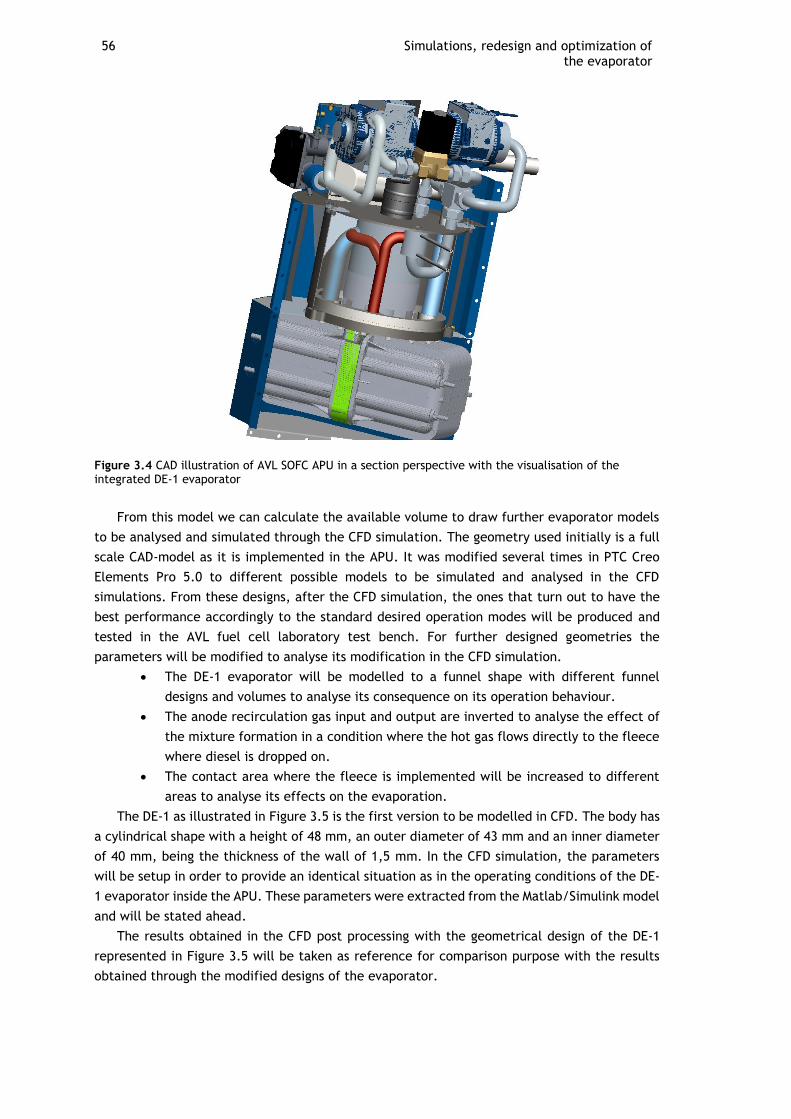
56 Simulations, redesign and optimization of the evaporator
Figure 3.4 CAD illustration of AVL SOFC APU in a section perspective with the visualisation of the integrated DE-1 evaporator
From this model we can calculate the available volume to draw further evaporator models
to be analysed and simulated through the CFD simulation. The geometry used initially is a full
scale CAD-model as it is implemented in the APU. It was modified several times in PTC Creo
Elements Pro 5.0 to different possible models to be simulated and analysed in the CFD
simulations. From these designs, after the CFD simulation, the ones that turn out to have the
best performance accordingly to the standard desired operation modes will be produced and
tested in the AVL fuel cell laboratory test bench. For further designed geometries the
parameters will be modified to analyse its modification in the CFD simulation.
The DE-1 evaporator will be modelled to a funnel shape with different funnel
designs and volumes to analyse its consequence on its operation behaviour.
The anode recirculation gas input and output are inverted to analyse the effect of
the mixture formation in a condition where the hot gas flows directly to the fleece
where diesel is dropped on.
The contact area where the fleece is implemented will be increased to different
areas to analyse its effects on the evaporation.
The DE-1 as illustrated in Figure 3.5 is the first version to be modelled in CFD. The body has
a cylindrical shape with a height of 48 mm, an outer diameter of 43 mm and an inner diameter
of 40 mm, being the thickness of the wall of 1,5 mm. In the CFD simulation, the parameters
will be setup in order to provide an identical situation as in the operating conditions of the DE-
1 evaporator inside the APU. These parameters were extracted from the Matlab/Simulink model
and will be stated ahead.
The results obtained in the CFD post processing with the geometrical design of the DE-1
represented in Figure 3.5 will be taken as reference for comparison purpose with the results
obtained through the modified designs of the evaporator.
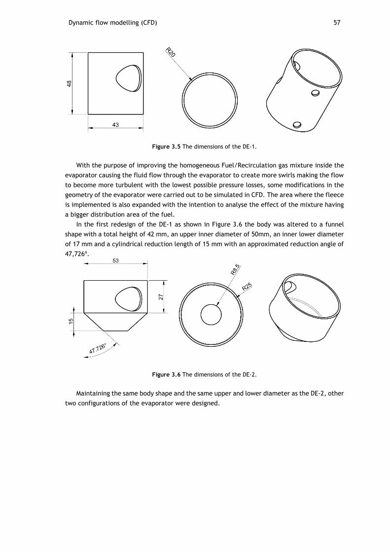
Dynamic flow modelling (CFD) 57
Figure 3.5 The dimensions of the DE-1.
With the purpose of improving the homogeneous Fuel/Recirculation gas mixture inside the
evaporator causing the fluid flow through the evaporator to create more swirls making the flow
to become more turbulent with the lowest possible pressure losses, some modifications in the
geometry of the evaporator were carried out to be simulated in CFD. The area where the fleece
is implemented is also expanded with the intention to analyse the effect of the mixture having
a bigger distribution area of the fuel.
In the first redesign of the DE-1 as shown in Figure 3.6 the body was altered to a funnel
shape with a total height of 42 mm, an upper inner diameter of 50mm, an inner lower diameter
of 17 mm and a cylindrical reduction length of 15 mm with an approximated reduction angle of
47,726º.
Figure 3.6 The dimensions of the DE-2.
Maintaining the same body shape and the same upper and lower diameter as the DE-2, other
two configurations of the evaporator were designed.
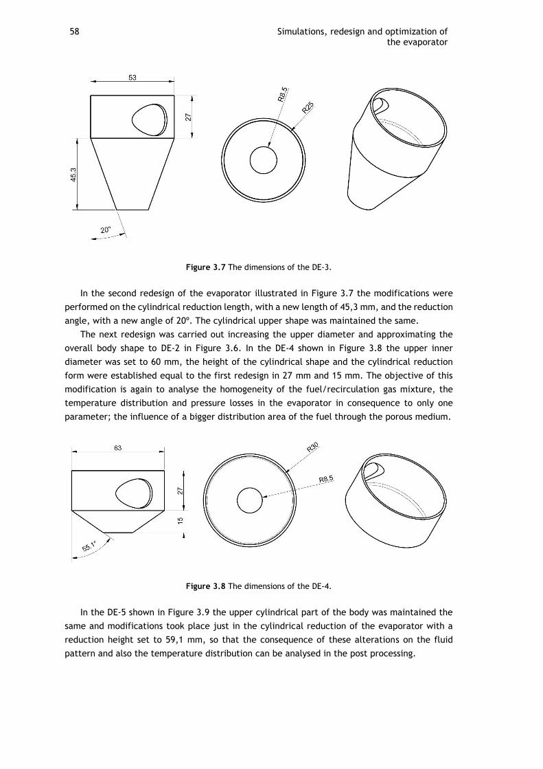
58 Simulations, redesign and optimization of the evaporator
Figure 3.7 The dimensions of the DE-3.
In the second redesign of the evaporator illustrated in Figure 3.7 the modifications were
performed on the cylindrical reduction length, with a new length of 45,3 mm, and the reduction
angle, with a new angle of 20º. The cylindrical upper shape was maintained the same.
The next redesign was carried out increasing the upper diameter and approximating the
overall body shape to DE-2 in Figure 3.6. In the DE-4 shown in Figure 3.8 the upper inner
diameter was set to 60 mm, the height of the cylindrical shape and the cylindrical reduction
form were established equal to the first redesign in 27 mm and 15 mm. The objective of this
modification is again to analyse the homogeneity of the fuel/recirculation gas mixture, the
temperature distribution and pressure losses in the evaporator in consequence to only one
parameter; the influence of a bigger distribution area of the fuel through the porous medium.
Figure 3.8 The dimensions of the DE-4.
In the DE-5 shown in Figure 3.9 the upper cylindrical part of the body was maintained the
same and modifications took place just in the cylindrical reduction of the evaporator with a
reduction height set to 59,1 mm, so that the consequence of these alterations on the fluid
pattern and also the temperature distribution can be analysed in the post processing.
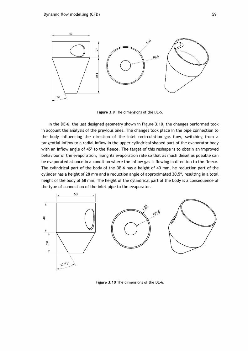
Dynamic flow modelling (CFD) 59
Figure 3.9 The dimensions of the DE-5.
In the DE-6, the last designed geometry shown in Figure 3.10, the changes performed took
in account the analysis of the previous ones. The changes took place in the pipe connection to
the body influencing the direction of the inlet recirculation gas flow, switching from a
tangential inflow to a radial inflow in the upper cylindrical shaped part of the evaporator body
with an inflow angle of 45º to the fleece. The target of this reshape is to obtain an improved
behaviour of the evaporation, rising its evaporation rate so that as much diesel as possible can
be evaporated at once in a condition where the inflow gas is flowing in direction to the fleece.
The cylindrical part of the body of the DE-6 has a height of 40 mm, he reduction part of the
cylinder has a height of 28 mm and a reduction angle of approximated 30,5º, resulting in a total
height of the body of 68 mm. The height of the cylindrical part of the body is a consequence of
the type of connection of the inlet pipe to the evaporator.
Figure 3.10 The dimensions of the DE-6.
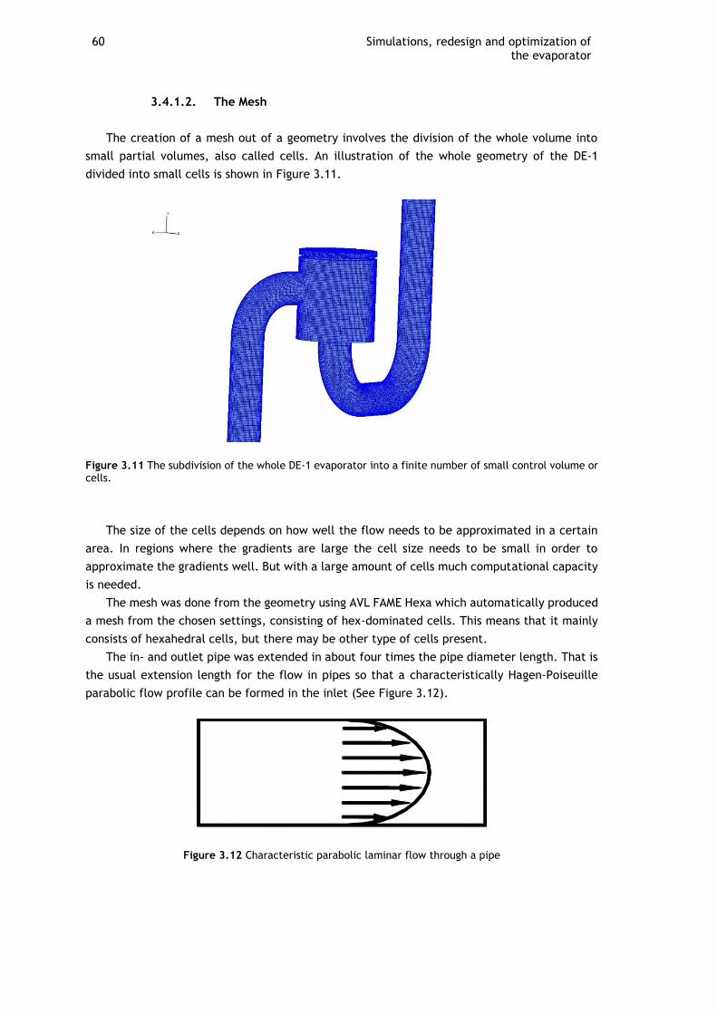
60 Simulations, redesign and optimization of the evaporator
3.4.1.2. The Mesh
The creation of a mesh out of a geometry involves the division of the whole volume into
small partial volumes, also called cells. An illustration of the whole geometry of the DE-1
divided into small cells is shown in Figure 3.11.
Figure 3.11 The subdivision of the whole DE-1 evaporator into a finite number of small control volume or cells.
The size of the cells depends on how well the flow needs to be approximated in a certain
area. In regions where the gradients are large the cell size needs to be small in order to
approximate the gradients well. But with a large amount of cells much computational capacity
is needed.
The mesh was done from the geometry using AVL FAME Hexa which automatically produced
a mesh from the chosen settings, consisting of hex-dominated cells. This means that it mainly
consists of hexahedral cells, but there may be other type of cells present.
The in- and outlet pipe was extended in about four times the pipe diameter length. That is
the usual extension length for the flow in pipes so that a characteristically Hagen-Poiseuille
parabolic flow profile can be formed in the inlet (See Figure 3.12).
Figure 3.12 Characteristic parabolic laminar flow through a pipe
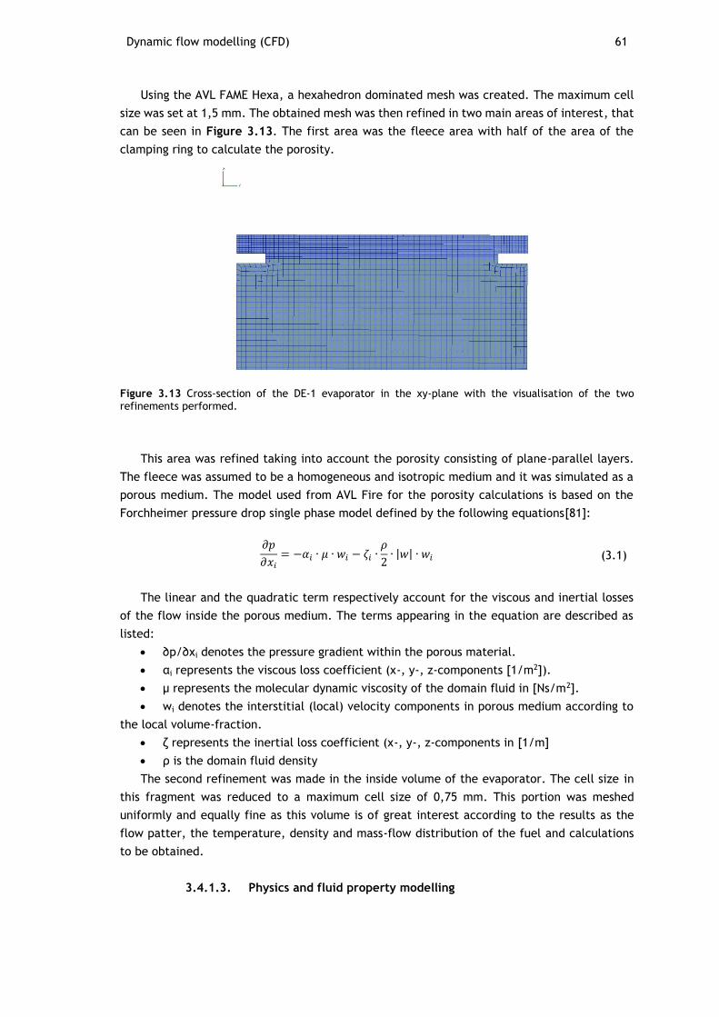
Dynamic flow modelling (CFD) 61
Using the AVL FAME Hexa, a hexahedron dominated mesh was created. The maximum cell
size was set at 1,5 mm. The obtained mesh was then refined in two main areas of interest, that
can be seen in Figure 3.13. The first area was the fleece area with half of the area of the
clamping ring to calculate the porosity.
Figure 3.13 Cross-section of the DE-1 evaporator in the xy-plane with the visualisation of the two refinements performed.
This area was refined taking into account the porosity consisting of plane-parallel layers.
The fleece was assumed to be a homogeneous and isotropic medium and it was simulated as a
porous medium. The model used from AVL Fire for the porosity calculations is based on the
Forchheimer pressure drop single phase model defined by the following equations[81]:
𝜕𝑝
𝜕𝑥𝑖
= −𝛼𝑖 ∙ 𝜇 ∙ 𝑤𝑖 − 𝜁𝑖 ∙𝜌
2∙ |𝑤| ∙ 𝑤𝑖 (3.1)
The linear and the quadratic term respectively account for the viscous and inertial losses
of the flow inside the porous medium. The terms appearing in the equation are described as
listed:
∂p/∂xi denotes the pressure gradient within the porous material.
αi represents the viscous loss coefficient (x-, y-, z-components [1/m2]).
μ represents the molecular dynamic viscosity of the domain fluid in [Ns/m2].
wi denotes the interstitial (local) velocity components in porous medium according to
the local volume-fraction.
ζ represents the inertial loss coefficient (x-, y-, z-components in [1/m]
ρ is the domain fluid density
The second refinement was made in the inside volume of the evaporator. The cell size in
this fragment was reduced to a maximum cell size of 0,75 mm. This portion was meshed
uniformly and equally fine as this volume is of great interest according to the results as the
flow patter, the temperature, density and mass-flow distribution of the fuel and calculations
to be obtained.
3.4.1.3. Physics and fluid property modelling
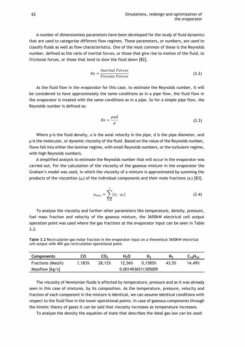
62 Simulations, redesign and optimization of the evaporator
A number of dimensionless parameters have been developed for the study of fluid dynamics
that are used to categorize different flow regimes. These parameters, or numbers, are used to
classify fluids as well as flow characteristics. One of the most common of these is the Reynolds
number, defined as the ratio of inertial forces, or those that give rise to motion of the fluid, to
frictional forces, or those that tend to slow the fluid down [82].
𝑅𝑒 =𝐼𝑛𝑒𝑟𝑡𝑖𝑎𝑙 𝐹𝑜𝑟𝑐𝑒𝑠
𝑉𝑖𝑠𝑐𝑜𝑢𝑠 𝐹𝑜𝑟𝑐𝑒𝑠 (3.2)
As the fluid flow in the evaporator for this case, to estimate the Reynolds number, it will
be considered to have approximately the same conditions as in a pipe flow, the fluid flow in
the evaporator is treated with the same conditions as in a pipe. So for a simple pipe flow, the
Reynolds number is defined as:
𝑅𝑒 =𝜌𝑢𝑑
𝜇 (3.3)
Where ρ is the fluid density, u is the axial velocity in the pipe, d is the pipe diameter, and
μ is the molecular, or dynamic viscosity of the fluid. Based on the value of the Reynolds number,
flows fall into either the laminar regime, with small Reynolds numbers, or the turbulent regime,
with high Reynolds numbers.
A simplified analysis to estimate the Reynolds number that will occur in the evaporator was
carried out. For the calculation of the viscosity of the gaseous mixture in the evaporator the
Graham’s model was used, in which the viscosity of a mixture is approximated by summing the
products of the viscosities (μi) of the individual components and their mole fractions (xi) [83].
𝜇𝑚𝑖𝑥 = ∑(𝑥𝑖 ∙ 𝜇𝑖)
𝑖
𝑖=0
(3.4)
To analyse the viscosity and further other parameters like temperature, density, pressure,
fuel mass fraction and velocity of the gaseous mixture, the 3650kW electrical cell output
operation point was used where the gas fractions at the evaporator input can be seen in Table
3.2:
Table 3.2 Recirculation gas molar fraction in the evaporator input on a theoretical 3650kW electrical cell output with 40% gas recirculation operational point.
Components CO CO2 H2O H2 N2 C16H34
Fractions (Mass%) 1,183% 28,12% 12,56% 0,1585% 43,5% 14,49%
Massflow [kg/s] 0.0014936511305009
The viscosity of Newtonian fluids is affected by temperature, pressure and as it was already
seen in this case of mixtures, by its composition. As the temperature, pressure, velocity and
fraction of each component in the mixture is identical, we can assume identical conditions with
respect to the fluid flow in the lower operational points. In case of gaseous components through
the kinetic theory of gases it can be said that viscosity increases as temperature increases.
To analyse the density the equation of state that describes the ideal gas law can be used:
Dynamic flow modelling (CFD) 63
𝑝𝑉 = 𝑛𝑅𝑇 (3.5)
Where p describes the pressure, V describes the volume, n the number of moles of a
substance, T the temperature and R the ideal gas constant. Through this relation it can be said
that the density decreases with the increase of temperature as the density is inverse
proportional to the volume [3]. Taking into account this analysis and the values of viscosity and
density for ambient pressure, temperatures and velocities occurring in the evaporator during
normal operation conditions, it can be estimated a Reynolds number approximately in a range
of 103 <Re<104 . Through this simplified analysis it can be considered to be in the presence of a
slightly turbulent and compressible internal flow.
The turbulent flow is irregular, chaotic, not completely predictable, and by definition
unsteady. Although a stationary approach was used, approximating the turbulent flow to a
stationary mode using a statistically stationary method that is explained in [84].
The random field U(x,t) is statistically stationary if all statistics are invariant under a shift
in time. It is characterised by the fluctuation u’ in the mean velocity �̅� [84]:
𝑢(𝑡) = �̅� + 𝑢′(𝑡) (3.6)
Direct numerical simulations of the turbulence provide a time-dependent solution of the
Navier-Stokes equations. This is only possible inside a very fine mesh that can take into account
the smallest possible vortex and requires a high computational effort.
For the industrial or technical practice, in which mainly macroscopic values are of interest,
turbulence models that represent a time-averaged position are used. Compared to the time-
dependent equations in this case the determination of the Reynolds stresses are additionally
required and are represented as follows [84]:
𝜏𝑖𝑗 = −𝜌𝑢′𝑖𝑢′𝑗̅̅ ̅̅ ̅̅ ̅ (3.7)
Of the classical models, it is distinguished between the so-called zero-, one-and two-
equation models depending on how many additional parameters and transport equations for
determination of the Reynolds stresses are needed. The mixing length and the k-ε are by far
the most widely used. These models are based on the presumption that there exists an analogy
between the action of viscous stresses and Reynolds stresses on the mean flow.
In order for the model to be able to provide meaningful results the effects of turbulence
need to be incorporated into the CFD model. This is done through the use of a turbulence
model.
3.4.1.4. The k-ε model
The simplest and most widely used two-equation model of turbulence is the k-ε model that
is characterised by the turbulent kinetic energy k and the rate of dissipation ε. The turbulent
kinetic energy is denoted by [84]:
𝑘 =1
2(𝑢′2̅̅ ̅̅ + 𝑣′2̅̅ ̅̅ + 𝑤′2̅̅ ̅̅ ̅) (3.8)
64 Simulations, redesign and optimization of the evaporator
Where (u,v,w) denote the velocity components normal to the faces (x,y,z). The rate of
dissipation per unit mass is the main destruction term in the turbulent kinetic energy and it is
given by [84]:
𝜀 = 2𝜈𝑒′𝑖𝑗 ∙ 𝑒′𝑖𝑗̅̅ ̅̅ ̅̅ ̅̅ ̅̅ ̅ (3.9)
Where ν is the dynamic viscosity and e’ij is the rate of deformation.
This model based on model transport equations for the turbulence kinetic energy (k) and
its dissipation rate (ε) is a semi empirical model. The turbulent kinetic energy and the
dissipation rate are obtained from the following transport equations that define the k-ε model
[82]:
Transport equation for k:
𝜕(𝜌𝑘)
𝜕𝑡+
𝜕
𝜕𝑥𝑖
(𝜌𝑢𝑖𝑘) =𝜕
𝜕𝑥𝑖
[(𝜇 +𝜇𝑡
𝜎𝑘
)𝜕𝑘
𝜕𝑥𝑖
] + 𝐺𝑘 − 𝜌𝜀 (3.10)
Transport equation for ε:
𝜕(𝜌𝜀)
𝜕𝑡+
𝜕
𝜕𝑥𝑖
(𝜌𝑢𝑖𝜀) =𝜕
𝜕𝑥𝑖
[(𝜇 +𝜇𝑡
𝜎𝜀
)𝜕𝜀
𝜕𝑥𝑖
] + 𝐶1
𝜀
𝑘𝐺𝑘 + 𝐶2𝜌
𝜀2
𝑘 (3.11)
Where the quantities C1, C2, are empirical constants, σk, σε are the turbulent Prandtl
numbers for k and respectively for ε and Gk represents a generation term for turbulence. It is
composed of products of velocity gradients and depends also on the turbulent viscosity as shown
in the equation below [82]:
𝐺𝑘 = 𝜇𝑡 (𝜕𝑢𝑖
𝜕𝑥𝑗
+𝜕𝑢𝑗
𝜕𝑥𝑖
)𝜕𝑢𝑗
𝜕𝑥𝑖
(3.12)
The term μt represents the turbulent viscosity that can be defined as:
𝜇𝑡 = 𝜌𝐶𝜇
𝑘2
𝜀 (3.13)
In this expression, the constant Cμ has a standard value of 0,09. The other experimentally
obtained constants assume the values of C1=1,44, C2=1,92, σk=1,0 and σε=1,3.
Finally in the solution process for the k-ε model the transport equations are solved for the
turbulence kinetic energy and dissipation rate. To compute the turbulent viscosity, μt, the
solutions for k and ε are used. Using the results for μt and k, the Reynolds stresses can be
computed for substitution into the momentum equations. Once the momentum equations have
been solved, the new velocity components are used to update the turbulence generation term,
Gk, and the process is repeated.
This model is a simple and complete turbulence model almost universally applicable and
represents a good compromise between accuracy and computational effort [85].
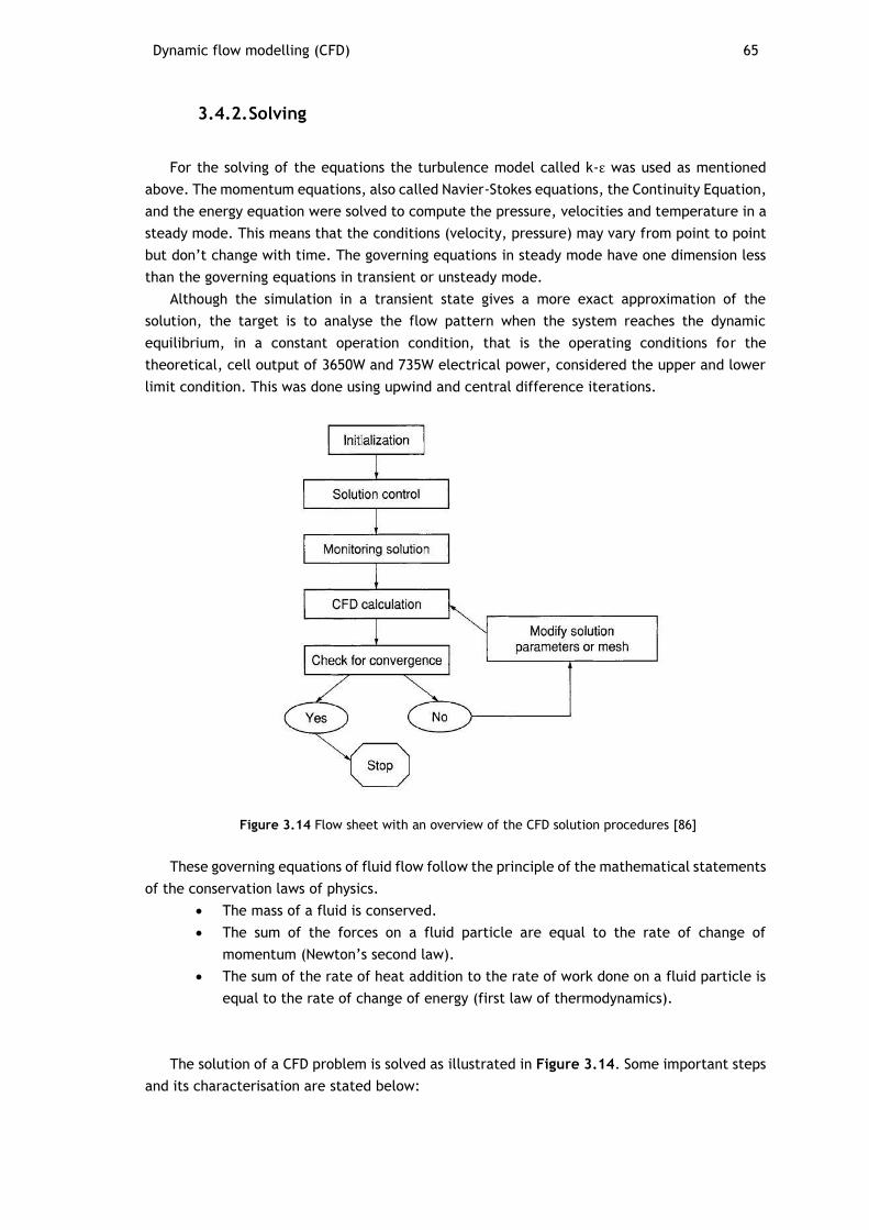
Dynamic flow modelling (CFD) 65
3.4.2. Solving
For the solving of the equations the turbulence model called k-ε was used as mentioned
above. The momentum equations, also called Navier-Stokes equations, the Continuity Equation,
and the energy equation were solved to compute the pressure, velocities and temperature in a
steady mode. This means that the conditions (velocity, pressure) may vary from point to point
but don’t change with time. The governing equations in steady mode have one dimension less
than the governing equations in transient or unsteady mode.
Although the simulation in a transient state gives a more exact approximation of the
solution, the target is to analyse the flow pattern when the system reaches the dynamic
equilibrium, in a constant operation condition, that is the operating conditions for the
theoretical, cell output of 3650W and 735W electrical power, considered the upper and lower
limit condition. This was done using upwind and central difference iterations.
Figure 3.14 Flow sheet with an overview of the CFD solution procedures [86]
These governing equations of fluid flow follow the principle of the mathematical statements
of the conservation laws of physics.
The mass of a fluid is conserved.
The sum of the forces on a fluid particle are equal to the rate of change of
momentum (Newton’s second law).
The sum of the rate of heat addition to the rate of work done on a fluid particle is
equal to the rate of change of energy (first law of thermodynamics).
The solution of a CFD problem is solved as illustrated in Figure 3.14. Some important steps
and its characterisation are stated below:
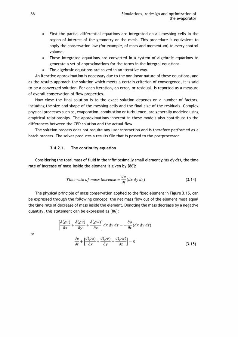
66 Simulations, redesign and optimization of the evaporator
First the partial differential equations are integrated on all meshing cells in the
region of interest of the geometry or the mesh. This procedure is equivalent to
apply the conservation law (for example, of mass and momentum) to every control
volume.
These integrated equations are converted in a system of algebraic equations to
generate a set of approximations for the terms in the integral equations
The algebraic equations are solved in an iterative way.
An iterative approximation is necessary due to the nonlinear nature of these equations, and
as the results approach the solution which meets a certain criterion of convergence, it is said
to be a converged solution. For each iteration, an error, or residual, is reported as a measure
of overall conservation of flow properties.
How close the final solution is to the exact solution depends on a number of factors,
including the size and shape of the meshing cells and the final size of the residuals. Complex
physical processes such as, evaporation, combustion or turbulence, are generally modeled using
empirical relationships. The approximations inherent in these models also contribute to the
differences between the CFD solution and the actual flow.
The solution process does not require any user interaction and is therefore performed as a
batch process. The solver produces a results file that is passed to the postprocessor.
3.4.2.1. The continuity equation
Considering the total mass of fluid in the infinitesimally small element ρ(dx dy dz), the time
rate of increase of mass inside the element is given by [86]:
𝑇𝑖𝑚𝑒 𝑟𝑎𝑡𝑒 𝑜𝑓 𝑚𝑎𝑠𝑠 𝑖𝑛𝑐𝑟𝑒𝑎𝑠𝑒 =𝜕𝜌
𝜕𝑡(𝑑𝑥 𝑑𝑦 𝑑𝑧) (3.14)
The physical principle of mass conservation applied to the fixed element in Figure 3.15, can
be expressed through the following concept: the net mass flow out of the element must equal
the time rate of decrease of mass inside the element. Denoting the mass decrease by a negative
quantity, this statement can be expressed as [86]:
[𝜕(𝜌𝑢)
𝜕𝑥+
𝜕(𝜌𝑣)
𝜕𝑦+
𝜕(𝜌𝑤)
𝜕𝑧] 𝑑𝑥 𝑑𝑦 𝑑𝑧 = −
𝜕𝜌
𝜕𝑡(𝑑𝑥 𝑑𝑦 𝑑𝑧)
or 𝜕𝜌
𝜕𝑡+ [
𝜕(𝜌𝑢)
𝜕𝑥+
𝜕(𝜌𝑣)
𝜕𝑦+
𝜕(𝜌𝑤)
𝜕𝑧] = 0
(3.15)
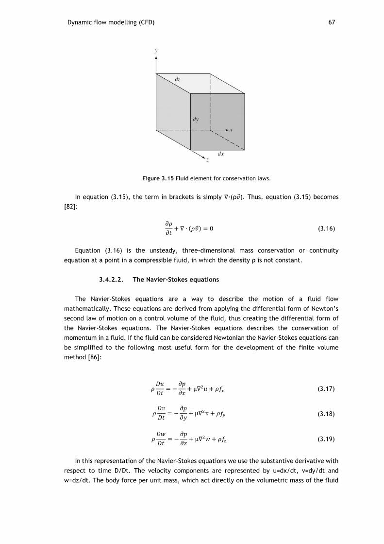
Dynamic flow modelling (CFD) 67
Figure 3.15 Fluid element for conservation laws.
In equation (3.15), the term in brackets is simply ∇∙(ρ�⃗�). Thus, equation (3.15) becomes
[82]:
𝜕𝜌
𝜕𝑡+ ∇ ∙ (𝜌�⃗�) = 0 (3.16)
Equation (3.16) is the unsteady, three-dimensional mass conservation or continuity
equation at a point in a compressible fluid, in which the density ρ is not constant.
3.4.2.2. The Navier-Stokes equations
The Navier-Stokes equations are a way to describe the motion of a fluid flow
mathematically. These equations are derived from applying the differential form of Newton’s
second law of motion on a control volume of the fluid, thus creating the differential form of
the Navier-Stokes equations. The Navier-Stokes equations describes the conservation of
momentum in a fluid. If the fluid can be considered Newtonian the Navier-Stokes equations can
be simplified to the following most useful form for the development of the finite volume
method [86]:
𝜌𝐷𝑢
𝐷𝑡= −
𝜕𝑝
𝜕𝑥+ μ∇2𝑢 + 𝜌𝑓𝑥 (3.17)
𝜌𝐷𝑣
𝐷𝑡= −
𝜕𝑝
𝜕𝑦+ μ∇2𝑣 + 𝜌𝑓𝑦 (3.18)
𝜌𝐷𝑤
𝐷𝑡= −
𝜕𝑝
𝜕𝑧+ μ∇2𝑤 + 𝜌𝑓𝑧 (3.19)
In this representation of the Navier-Stokes equations we use the substantive derivative with
respect to time D/Dt. The velocity components are represented by u=dx/dt, v=dy/dt and
w=dz/dt. The body force per unit mass, which act directly on the volumetric mass of the fluid
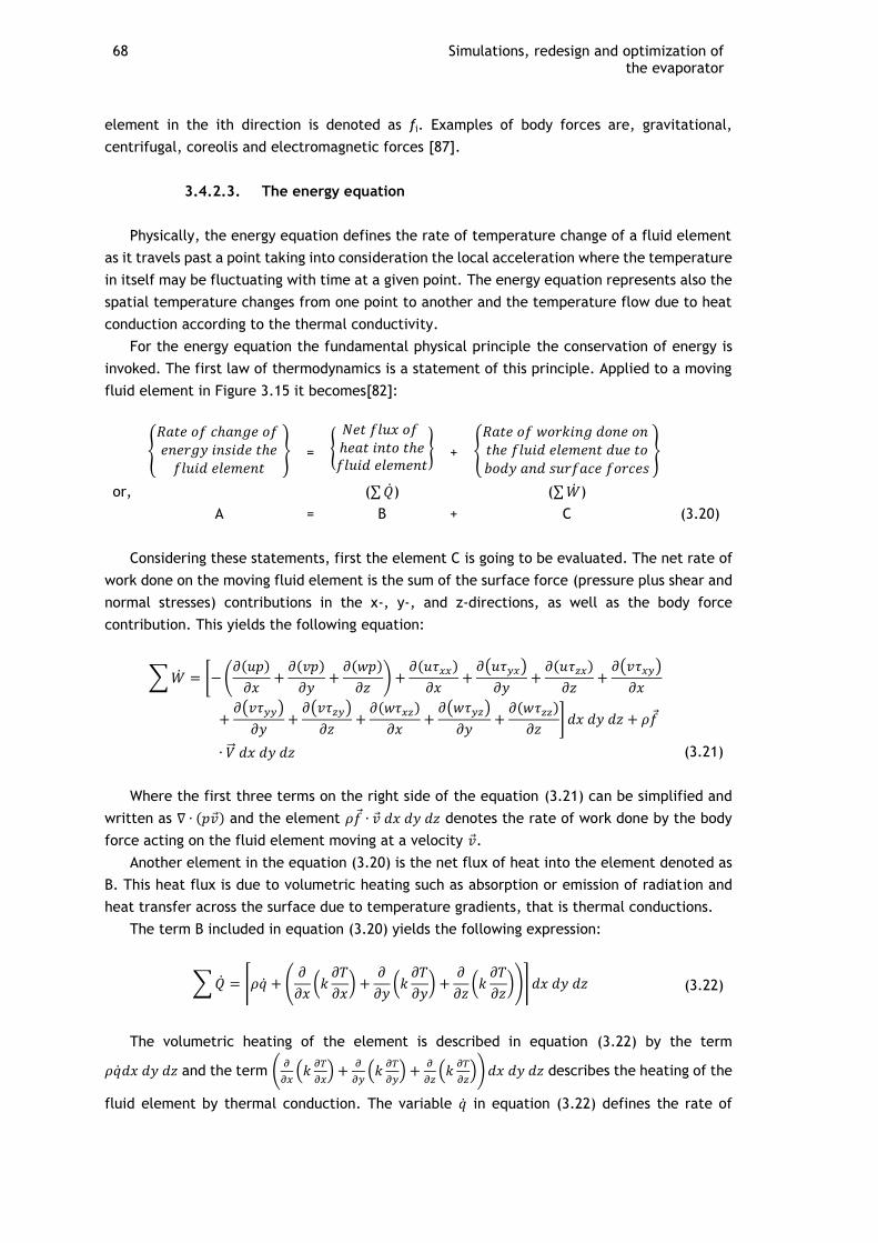
68 Simulations, redesign and optimization of the evaporator
element in the ith direction is denoted as fi. Examples of body forces are, gravitational,
centrifugal, coreolis and electromagnetic forces [87].
3.4.2.3. The energy equation
Physically, the energy equation defines the rate of temperature change of a fluid element
as it travels past a point taking into consideration the local acceleration where the temperature
in itself may be fluctuating with time at a given point. The energy equation represents also the
spatial temperature changes from one point to another and the temperature flow due to heat
conduction according to the thermal conductivity.
For the energy equation the fundamental physical principle the conservation of energy is
invoked. The first law of thermodynamics is a statement of this principle. Applied to a moving
fluid element in Figure 3.15 it becomes[82]:
{
𝑅𝑎𝑡𝑒 𝑜𝑓 𝑐ℎ𝑎𝑛𝑔𝑒 𝑜𝑓 𝑒𝑛𝑒𝑟𝑔𝑦 𝑖𝑛𝑠𝑖𝑑𝑒 𝑡ℎ𝑒
𝑓𝑙𝑢𝑖𝑑 𝑒𝑙𝑒𝑚𝑒𝑛𝑡} = {
𝑁𝑒𝑡 𝑓𝑙𝑢𝑥 𝑜𝑓 ℎ𝑒𝑎𝑡 𝑖𝑛𝑡𝑜 𝑡ℎ𝑒
𝑓𝑙𝑢𝑖𝑑 𝑒𝑙𝑒𝑚𝑒𝑛𝑡} + {
𝑅𝑎𝑡𝑒 𝑜𝑓 𝑤𝑜𝑟𝑘𝑖𝑛𝑔 𝑑𝑜𝑛𝑒 𝑜𝑛 𝑡ℎ𝑒 𝑓𝑙𝑢𝑖𝑑 𝑒𝑙𝑒𝑚𝑒𝑛𝑡 𝑑𝑢𝑒 𝑡𝑜
𝑏𝑜𝑑𝑦 𝑎𝑛𝑑 𝑠𝑢𝑟𝑓𝑎𝑐𝑒 𝑓𝑜𝑟𝑐𝑒𝑠}
or, (∑ �̇�) (∑ �̇�)
A = B + C (3.20)
Considering these statements, first the element C is going to be evaluated. The net rate of
work done on the moving fluid element is the sum of the surface force (pressure plus shear and
normal stresses) contributions in the x-, y-, and z-directions, as well as the body force
contribution. This yields the following equation:
∑ �̇� = [− (𝜕(𝑢𝑝)
𝜕𝑥+
𝜕(𝑣𝑝)
𝜕𝑦+
𝜕(𝑤𝑝)
𝜕𝑧) +
𝜕(𝑢𝜏𝑥𝑥)
𝜕𝑥+
𝜕(𝑢𝜏𝑦𝑥)
𝜕𝑦+
𝜕(𝑢𝜏𝑧𝑥)
𝜕𝑧+
𝜕(𝑣𝜏𝑥𝑦)
𝜕𝑥
+𝜕(𝑣𝜏𝑦𝑦)
𝜕𝑦+
𝜕(𝑣𝜏𝑧𝑦)
𝜕𝑧+
𝜕(𝑤𝜏𝑥𝑧)
𝜕𝑥+
𝜕(𝑤𝜏𝑦𝑧)
𝜕𝑦+
𝜕(𝑤𝜏𝑧𝑧)
𝜕𝑧] 𝑑𝑥 𝑑𝑦 𝑑𝑧 + 𝜌𝑓
∙ �⃗⃗� 𝑑𝑥 𝑑𝑦 𝑑𝑧 (3.21)
Where the first three terms on the right side of the equation (3.21) can be simplified and
written as ∇ ∙ (𝑝�⃗�) and the element 𝜌𝑓 ∙ �⃗� 𝑑𝑥 𝑑𝑦 𝑑𝑧 denotes the rate of work done by the body
force acting on the fluid element moving at a velocity �⃗�.
Another element in the equation (3.20) is the net flux of heat into the element denoted as
B. This heat flux is due to volumetric heating such as absorption or emission of radiation and
heat transfer across the surface due to temperature gradients, that is thermal conductions.
The term B included in equation (3.20) yields the following expression:
∑ �̇� = [𝜌�̇� + (𝜕
𝜕𝑥(𝑘
𝜕𝑇
𝜕𝑥) +
𝜕
𝜕𝑦(𝑘
𝜕𝑇
𝜕𝑦) +
𝜕
𝜕𝑧(𝑘
𝜕𝑇
𝜕𝑧))] 𝑑𝑥 𝑑𝑦 𝑑𝑧 (3.22)
The volumetric heating of the element is described in equation (3.22) by the term
𝜌�̇�𝑑𝑥 𝑑𝑦 𝑑𝑧 and the term (𝜕
𝜕𝑥(𝑘
𝜕𝑇
𝜕𝑥) +
𝜕
𝜕𝑦(𝑘
𝜕𝑇
𝜕𝑦) +
𝜕
𝜕𝑧(𝑘
𝜕𝑇
𝜕𝑧)) 𝑑𝑥 𝑑𝑦 𝑑𝑧 describes the heating of the
fluid element by thermal conduction. The variable �̇� in equation (3.22) defines the rate of
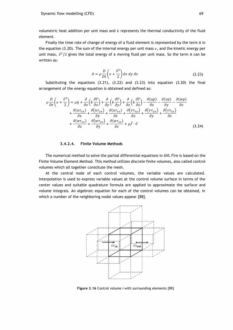
Dynamic flow modelling (CFD) 69
volumetric heat addition per unit mass and 𝑘 represents the thermal conductivity of the fluid
element.
Finally the time rate of change of energy of a fluid element is represented by the term A in
the equation (3.20). The sum of the internal energy per unit mass 𝑒, and the kinetic energy per
unit mass, �⃗�2/2 gives the total energy of a moving fluid per unit mass. So the term A can be
written as:
𝐴 = 𝜌𝐷
𝐷𝑡(𝑒 +
�⃗�2
2) 𝑑𝑥 𝑑𝑦 𝑑𝑧 (3.23)
Substituting the equations (3.21), (3.22) and (3.23) into equation (3.20) the final
arrangement of the energy equation is obtained and defined as:
𝜌𝐷
𝐷𝑡(𝑒 +
�⃗�2
2) = 𝜌�̇� +
𝜕
𝜕𝑥(𝑘
𝜕𝑇
𝜕𝑥) +
𝜕
𝜕𝑦(𝑘
𝜕𝑇
𝜕𝑦) +
𝜕
𝜕𝑧(𝑘
𝜕𝑇
𝜕𝑧) −
𝜕(𝑢𝑝)
𝜕𝑥−
𝜕(𝑣𝑝)
𝜕𝑦−
𝜕(𝑤𝑝)
𝜕𝑧
+𝜕(𝑢𝜏𝑥𝑥)
𝜕𝑥+
𝜕(𝑢𝜏𝑦𝑥)
𝜕𝑦+
𝜕(𝑢𝜏𝑧𝑥)
𝜕𝑧+
𝜕(𝑣𝜏𝑥𝑦)
𝜕𝑥+
𝜕(𝑣𝜏𝑦𝑦)
𝜕𝑦+
𝜕(𝑣𝜏𝑧𝑦)
𝜕𝑧
+𝜕(𝑤𝜏𝑥𝑧)
𝜕𝑥+
𝜕(𝑤𝜏𝑦𝑧)
𝜕𝑦+
𝜕(𝑤𝜏𝑧𝑧)
𝜕𝑧+ 𝜌𝑓 ∙ �⃗�
(3.24)
3.4.2.4. Finite Volume Methods
The numerical method to solve the partial differential equations in AVL Fire is based on the
Finite Volume Element Method. This method utilizes discrete finite volumes, also called control
volumes which all together constitute the mesh.
At the central node of each control volumes, the variable values are calculated.
Interpolation is used to express variable values at the control volume surface in terms of the
center values and suitable quadrature formula are applied to approximate the surface and
volume integrals. An algebraic equation for each of the control volumes can be obtained, in
which a number of the neighboring nodal values appear [88].
Figure 3.16 Control volume i with surrounding elements [89]
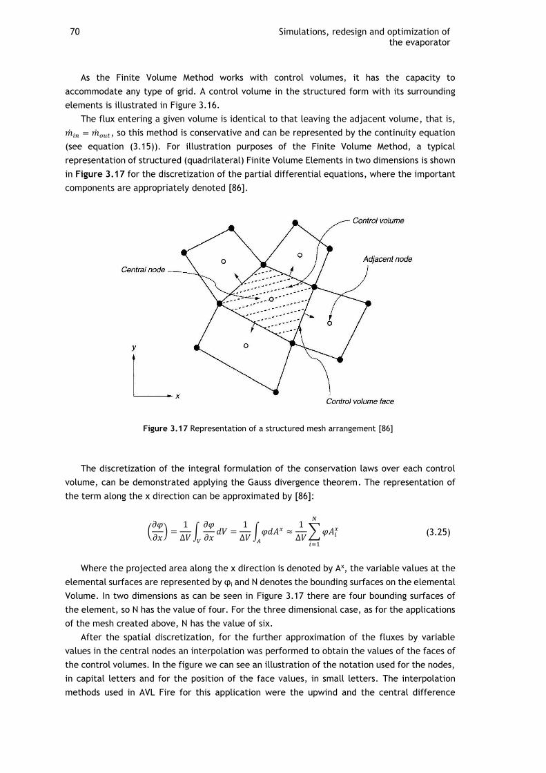
70 Simulations, redesign and optimization of the evaporator
As the Finite Volume Method works with control volumes, it has the capacity to
accommodate any type of grid. A control volume in the structured form with its surrounding
elements is illustrated in Figure 3.16.
The flux entering a given volume is identical to that leaving the adjacent volume, that is,
�̇�𝑖𝑛 = �̇�𝑜𝑢𝑡, so this method is conservative and can be represented by the continuity equation
(see equation (3.15)). For illustration purposes of the Finite Volume Method, a typical
representation of structured (quadrilateral) Finite Volume Elements in two dimensions is shown
in Figure 3.17 for the discretization of the partial differential equations, where the important
components are appropriately denoted [86].
Figure 3.17 Representation of a structured mesh arrangement [86]
The discretization of the integral formulation of the conservation laws over each control
volume, can be demonstrated applying the Gauss divergence theorem. The representation of
the term along the x direction can be approximated by [86]:
(𝜕𝜑
𝜕𝑥) =
1
∆𝑉∫
𝜕𝜑
𝜕𝑥𝑑𝑉
𝑉
=1
∆𝑉∫ 𝜑𝑑𝐴𝑥
𝐴
≈1
∆𝑉∑ 𝜑𝐴𝑖
𝑥
𝑁
𝑖=1
(3.25)
Where the projected area along the x direction is denoted by Ax, the variable values at the
elemental surfaces are represented by φi and N denotes the bounding surfaces on the elemental
Volume. In two dimensions as can be seen in Figure 3.17 there are four bounding surfaces of
the element, so N has the value of four. For the three dimensional case, as for the applications
of the mesh created above, N has the value of six.
After the spatial discretization, for the further approximation of the fluxes by variable
values in the central nodes an interpolation was performed to obtain the values of the faces of
the control volumes. In the figure we can see an illustration of the notation used for the nodes,
in capital letters and for the position of the face values, in small letters. The interpolation
methods used in AVL Fire for this application were the upwind and the central difference
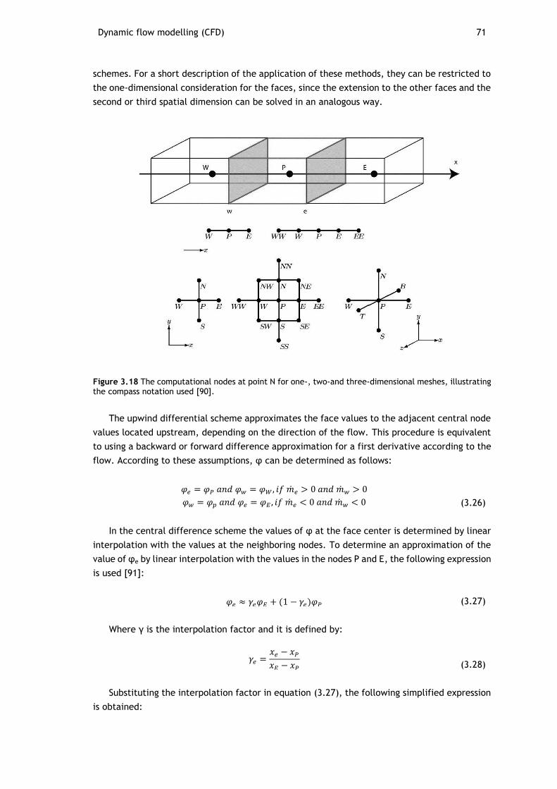
Dynamic flow modelling (CFD) 71
schemes. For a short description of the application of these methods, they can be restricted to
the one-dimensional consideration for the faces, since the extension to the other faces and the
second or third spatial dimension can be solved in an analogous way.
Figure 3.18 The computational nodes at point N for one-, two-and three-dimensional meshes, illustrating the compass notation used [90].
The upwind differential scheme approximates the face values to the adjacent central node
values located upstream, depending on the direction of the flow. This procedure is equivalent
to using a backward or forward difference approximation for a first derivative according to the
flow. According to these assumptions, φ can be determined as follows:
𝜑𝑒 = 𝜑𝑃 𝑎𝑛𝑑 𝜑𝑤 = 𝜑𝑊 , 𝑖𝑓 �̇�𝑒 > 0 𝑎𝑛𝑑 �̇�𝑤 > 0
𝜑𝑤 = 𝜑𝑝 𝑎𝑛𝑑 𝜑𝑒 = 𝜑𝐸 , 𝑖𝑓 �̇�𝑒 < 0 𝑎𝑛𝑑 �̇�𝑤 < 0 (3.26)
In the central difference scheme the values of φ at the face center is determined by linear
interpolation with the values at the neighboring nodes. To determine an approximation of the
value of φe by linear interpolation with the values in the nodes P and E, the following expression
is used [91]:
𝜑𝑒 ≈ 𝛾𝑒𝜑𝐸 + (1 − 𝛾𝑒)𝜑𝑃 (3.27)
Where γ is the interpolation factor and it is defined by:
𝛾𝑒 =𝑥𝑒 − 𝑥𝑃
𝑥𝐸 − 𝑥𝑃
(3.28)
Substituting the interpolation factor in equation (3.27), the following simplified expression
is obtained:
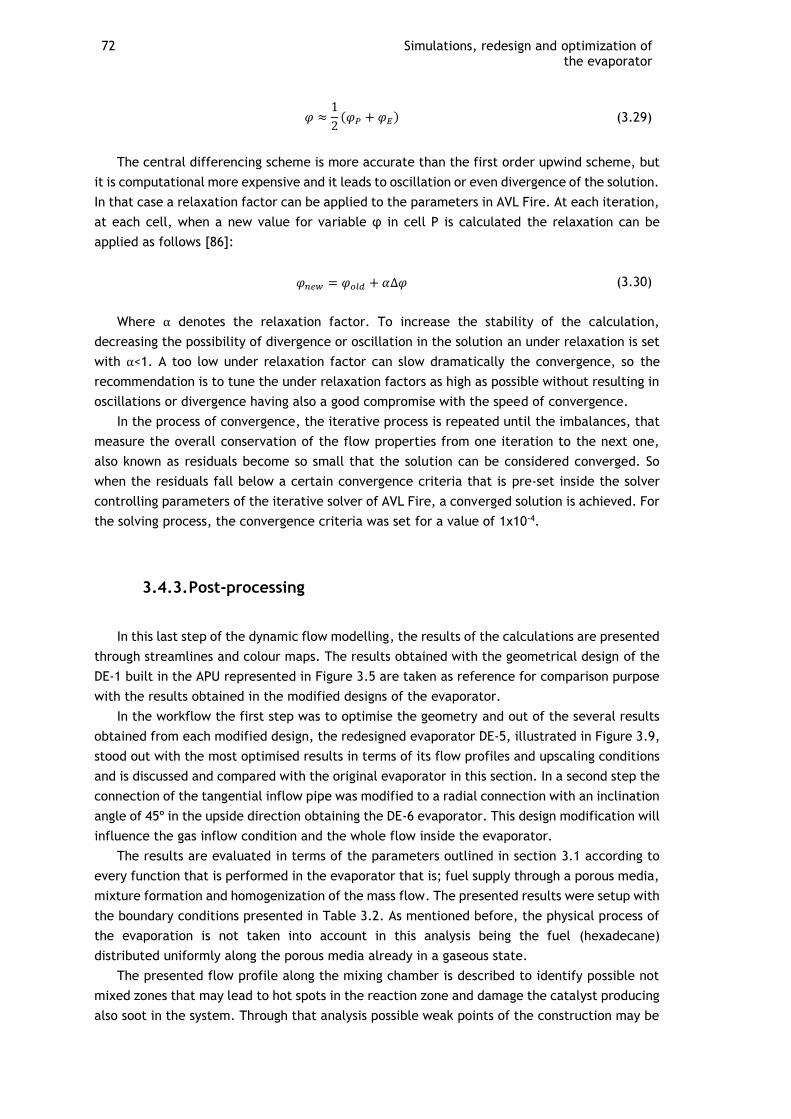
72 Simulations, redesign and optimization of the evaporator
𝜑 ≈1
2(𝜑𝑃 + 𝜑𝐸) (3.29)
The central differencing scheme is more accurate than the first order upwind scheme, but
it is computational more expensive and it leads to oscillation or even divergence of the solution.
In that case a relaxation factor can be applied to the parameters in AVL Fire. At each iteration,
at each cell, when a new value for variable φ in cell P is calculated the relaxation can be
applied as follows [86]:
𝜑𝑛𝑒𝑤 = 𝜑𝑜𝑙𝑑 + 𝛼∆𝜑 (3.30)
Where α denotes the relaxation factor. To increase the stability of the calculation,
decreasing the possibility of divergence or oscillation in the solution an under relaxation is set
with α<1. A too low under relaxation factor can slow dramatically the convergence, so the
recommendation is to tune the under relaxation factors as high as possible without resulting in
oscillations or divergence having also a good compromise with the speed of convergence.
In the process of convergence, the iterative process is repeated until the imbalances, that
measure the overall conservation of the flow properties from one iteration to the next one,
also known as residuals become so small that the solution can be considered converged. So
when the residuals fall below a certain convergence criteria that is pre-set inside the solver
controlling parameters of the iterative solver of AVL Fire, a converged solution is achieved. For
the solving process, the convergence criteria was set for a value of 1x10⁻⁴.
3.4.3. Post-processing
In this last step of the dynamic flow modelling, the results of the calculations are presented
through streamlines and colour maps. The results obtained with the geometrical design of the
DE-1 built in the APU represented in Figure 3.5 are taken as reference for comparison purpose
with the results obtained in the modified designs of the evaporator.
In the workflow the first step was to optimise the geometry and out of the several results
obtained from each modified design, the redesigned evaporator DE-5, illustrated in Figure 3.9,
stood out with the most optimised results in terms of its flow profiles and upscaling conditions
and is discussed and compared with the original evaporator in this section. In a second step the
connection of the tangential inflow pipe was modified to a radial connection with an inclination
angle of 45º in the upside direction obtaining the DE-6 evaporator. This design modification will
influence the gas inflow condition and the whole flow inside the evaporator.
The results are evaluated in terms of the parameters outlined in section 3.1 according to
every function that is performed in the evaporator that is; fuel supply through a porous media,
mixture formation and homogenization of the mass flow. The presented results were setup with
the boundary conditions presented in Table 3.2. As mentioned before, the physical process of
the evaporation is not taken into account in this analysis being the fuel (hexadecane)
distributed uniformly along the porous media already in a gaseous state.
The presented flow profile along the mixing chamber is described to identify possible not
mixed zones that may lead to hot spots in the reaction zone and damage the catalyst producing
also soot in the system. Through that analysis possible weak points of the construction may be
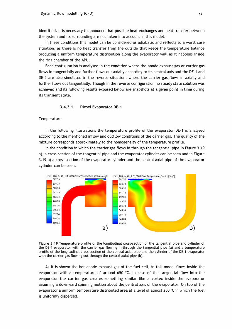
Dynamic flow modelling (CFD) 73
identified. It is necessary to announce that possible heat exchanges and heat transfer between
the system and its surrounding are not taken into account in this model.
In these conditions this model can be considered as adiabatic and reflects so a worst case
situation, as there is no heat transfer from the outside that keeps the temperature balance
producing a uniform temperature distribution along the evaporator wall as it happens inside
the ring chamber of the APU.
Each configuration is analysed in the condition where the anode exhaust gas or carrier gas
flows in tangentially and further flows out axially according to its central axis and the DE-1 and
DE-5 are also simulated in the reverse situation, where the carrier gas flows in axially and
further flows out tangentially. Though in the reverse configuration no steady state solution was
achieved and its following results exposed below are snapshots at a given point in time during
its transient state.
3.4.3.1. Diesel Evaporator DE-1
Temperature
In the following illustrations the temperature profile of the evaporator DE-1 is analysed
according to the mentioned inflow and outflow conditions of the carrier gas. The quality of the
mixture corresponds approximately to the homogeneity of the temperature profile.
In the condition in which the carrier gas flows in through the tangential pipe in Figure 3.19
a), a cross-section of the tangential pipe and the evaporator cylinder can be seen and in Figure
3.19 b) a cross section of the evaporator cylinder and the central axial pipe of the evaporator
cylinder can be seen.
Figure 3.19 Temperature profile of the longitudinal cross-section of the tangential pipe and cylinder of the DE-1 evaporator with the carrier gas flowing in through the tangential pipe (a) and a temperature profile of the longitudinal cross-section of the central axial pipe and the cylinder of the DE-1 evaporator with the carrier gas flowing out through the central axial pipe (b).
As it is shown the hot anode exhaust gas of the fuel cell, in this model flows inside the
evaporator with a temperature of around 650 ºC. In case of the tangential flow into the
evaporator the carrier gas creates something similar like a vortex inside the evaporator
assuming a downward spinning motion about the central axis of the evaporator. On top of the
evaporator a uniform temperature distributed area at a level of almost 250 ºC in which the fuel
is uniformly dispersed.
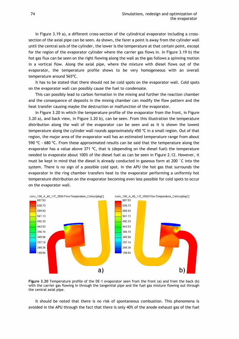
74 Simulations, redesign and optimization of the evaporator
In Figure 3.19 a), a different cross-section of the cylindrical evaporator including a cross-
section of the axial pipe can be seen. As shown, the farer a point is away from the cylinder wall
until the central axis of the cylinder, the lower is the temperature at that certain point, except
for the region of the evaporator cylinder where the carrier gas flows in. In Figure 3.19 b) the
hot gas flux can be seen on the right flowing along the wall as the gas follows a spinning motion
in a vortical flow. Along the axial pipe, where the mixture with diesel flows out of the
evaporator, the temperature profile shows to be very homogeneous with an overall
temperature around 565ºC.
It has to be stated that there should not be cold spots on the evaporator wall. Cold spots
on the evaporator wall can possibly cause the fuel to condensate.
This can possibly lead to carbon formation in the mixing and further the reaction chamber
and the consequence of deposits in the mixing chamber can modify the flow pattern and the
heat transfer causing maybe the destruction or malfunction of the evaporator.
In Figure 3.20 in which the temperature profile of the evaporator from the front, in Figure
3.20 a), and back view, in Figure 3.20 b), can be seen. From this illustration the temperature
distribution along the wall of the evaporator can be seen and as it is shown the lowest
temperature along the cylinder wall rounds approximately 450 ºC in a small region. Out of that
region, the major area of the evaporator wall has an estimated temperature range from about
590 ºC - 680 ºC. From these approximated results can be said that the temperature along the
evaporator has a value above 371 ºC, that is (depending on the diesel fuel) the temperature
needed to evaporate about 100% of the diesel fuel as can be seen in Figure 2.12. However, it
must be kept in mind that the diesel is already conducted in gaseous form at 200 °C into the
system. There is no sign of a possible cold spot. In the APU the hot gas that surrounds the
evaporator in the ring chamber transfers heat to the evaporator performing a uniformly hot
temperature distribution on the evaporator becoming even less possible for cold spots to occur
on the evaporator wall.
Figure 3.20 Temperature profile of the DE-1 evaporator seen from the front (a) and from the back (b) with the carrier gas flowing in through the tangential pipe and the fuel gas mixture flowing out through the central axial pipe.
It should be noted that there is no risk of spontaneous combustion. This phenomena is
avoided in the APU through the fact that there is only 40% of the anode exhaust gas of the fuel
Dynamic flow modelling (CFD) 75
cell, that is no air or oxidizer is present in the mixture. The air will be added to the mixture in
an under stoichiometric relation of 0,36 oxygen to fuel ratio before it reaches the reaction zone
in the reformer as can be seen in Figure 2.15.
In Figure 3.21 b) a cross-section of the evaporator is represented in the situation in which
the carrier gas flows into the evaporator through the central axial pipe and flows out of the
evaporator through the tangential pipe in Figure 3.21 a). Here it can be seen that the
temperature distribution inside the evaporator is mainly in a range between 450 ºC and 550 ºC
except for the specific region where the carrier gas flows inside the evaporator where the
temperature assumes values above 600 ºC.
Figure 3.21 Temperature profile of the longitudinal cross-section of the tangential pipe and cylinder of DE-1 with the carrier gas flowing in through the tangential pipe (a) and a temperature profile of the cross-section of the central axial pipe and the cylinder of DE-1 with the carrier gas flowing out through the central axial pipe (b).
In this snapshot of the transient solution the carrier gas flowing inside the evaporator
streams on the porous media with a slight tendency to the left heating it up through its
impinging condition. It has to be kept in mind that the solution obtained is not stationary. Due
to the fact that the carrier gas goes through a curvature before flowing inside the evaporator,
that can lead to a slight flow separation in that area and also that the tangential pipe is
positioned on the left side from the perspective on Figure 3.21 the flow tends to have an
inclination the left side following the trajectory that presents less resistance. This condition
leads to a sudden quick temperature reduction close to 470 ºC around two-thirds of the
evaporator.
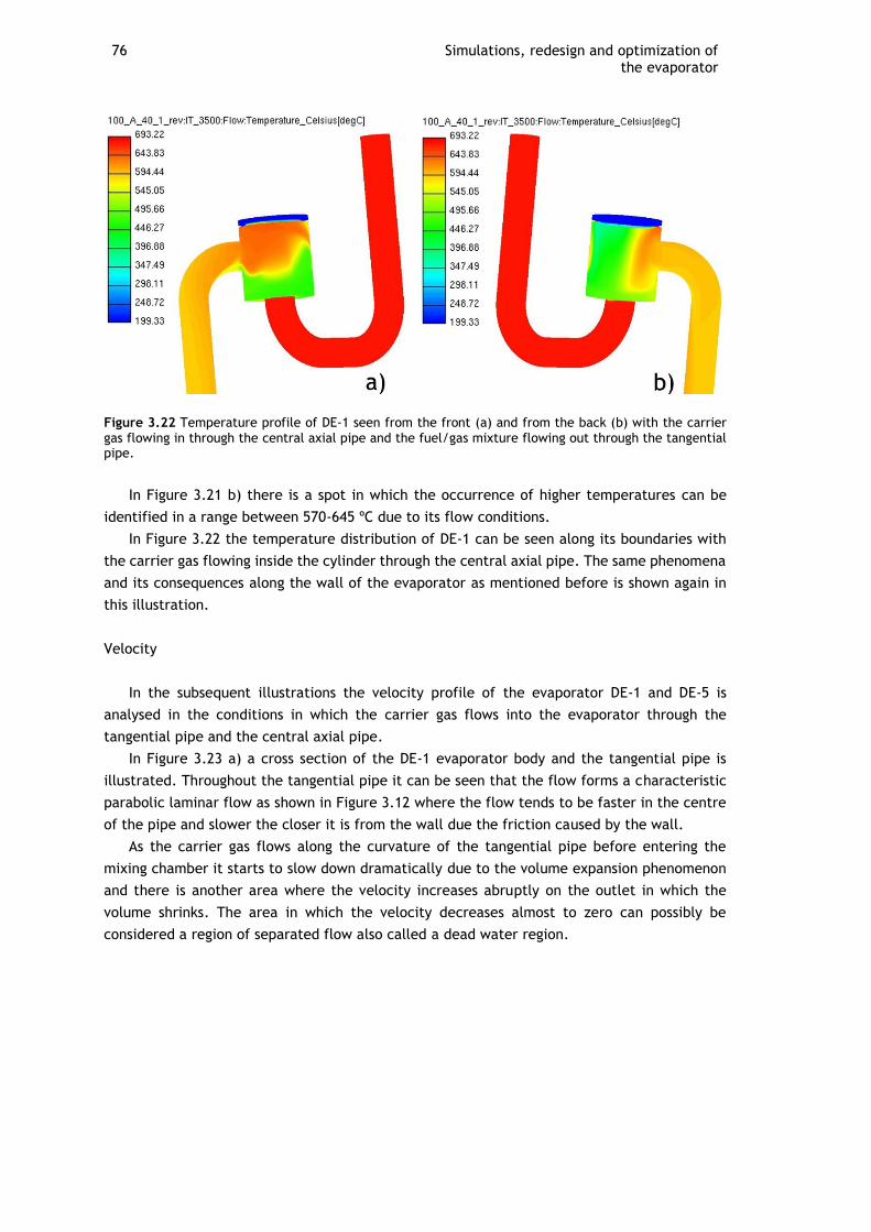
76 Simulations, redesign and optimization of the evaporator
Figure 3.22 Temperature profile of DE-1 seen from the front (a) and from the back (b) with the carrier gas flowing in through the central axial pipe and the fuel/gas mixture flowing out through the tangential pipe.
In Figure 3.21 b) there is a spot in which the occurrence of higher temperatures can be
identified in a range between 570-645 ºC due to its flow conditions.
In Figure 3.22 the temperature distribution of DE-1 can be seen along its boundaries with
the carrier gas flowing inside the cylinder through the central axial pipe. The same phenomena
and its consequences along the wall of the evaporator as mentioned before is shown again in
this illustration.
Velocity
In the subsequent illustrations the velocity profile of the evaporator DE-1 and DE-5 is
analysed in the conditions in which the carrier gas flows into the evaporator through the
tangential pipe and the central axial pipe.
In Figure 3.23 a) a cross section of the DE-1 evaporator body and the tangential pipe is
illustrated. Throughout the tangential pipe it can be seen that the flow forms a characteristic
parabolic laminar flow as shown in Figure 3.12 where the flow tends to be faster in the centre
of the pipe and slower the closer it is from the wall due the friction caused by the wall.
As the carrier gas flows along the curvature of the tangential pipe before entering the
mixing chamber it starts to slow down dramatically due to the volume expansion phenomenon
and there is another area where the velocity increases abruptly on the outlet in which the
volume shrinks. The area in which the velocity decreases almost to zero can possibly be
considered a region of separated flow also called a dead water region.
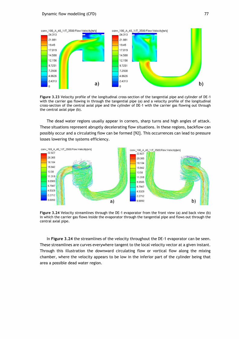
Dynamic flow modelling (CFD) 77
Figure 3.23 Velocity profile of the longitudinal cross-section of the tangential pipe and cylinder of DE-1 with the carrier gas flowing in through the tangential pipe (a) and a velocity profile of the longitudinal cross-section of the central axial pipe and the cylinder of DE-1 with the carrier gas flowing out through the central axial pipe (b).
The dead water regions usually appear in corners, sharp turns and high angles of attack.
These situations represent abruptly decelerating flow situations. In these regions, backflow can
possibly occur and a circulating flow can be formed [92]. This occurrences can lead to pressure
losses lowering the systems efficiency.
Figure 3.24 Velocity streamlines through the DE-1 evaporator from the front view (a) and back view (b) in which the carrier gas flows inside the evaporator through the tangential pipe and flows out through the central axial pipe.
In Figure 3.24 the streamlines of the velocity throughout the DE-1 evaporator can be seen.
These streamlines are curves everywhere tangent to the local velocity vector at a given instant.
Through this illustration the downward circulating flow or vortical flow along the mixing
chamber, where the velocity appears to be low in the inferior part of the cylinder being that
area a possible dead water region.
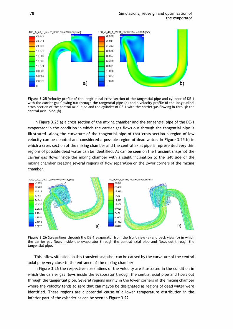
78 Simulations, redesign and optimization of the evaporator
Figure 3.25 Velocity profile of the longitudinal cross-section of the tangential pipe and cylinder of DE-1 with the carrier gas flowing out through the tangential pipe (a) and a velocity profile of the longitudinal cross-section of the central axial pipe and the cylinder of DE-1 with the carrier gas flowing in through the central axial pipe (b).
In Figure 3.25 a) a cross section of the mixing chamber and the tangential pipe of the DE-1
evaporator in the condition in which the carrier gas flows out through the tangential pipe is
illustrated. Along the curvature of the tangential pipe of that cross-section a region of low
velocity can be denoted and considered a possible region of dead water. In Figure 3.25 b) in
which a cross section of the mixing chamber and the central axial pipe is represented very thin
regions of possible dead water can be identified. As can be seen on the transient snapshot the
carrier gas flows inside the mixing chamber with a slight inclination to the left side of the
mixing chamber creating several regions of flow separation on the lower corners of the mixing
chamber.
Figure 3.26 Streamlines through the DE-1 evaporator from the front view (a) and back view (b) in which the carrier gas flows inside the evaporator through the central axial pipe and flows out through the tangential pipe.
This inflow situation on this transient snapshot can be caused by the curvature of the central
axial pipe very close to the entrance of the mixing chamber.
In Figure 3.26 the respective streamlines of the velocity are illustrated in the condition in
which the carrier gas flows inside the evaporator through the central axial pipe and flows out
through the tangential pipe. Several regions mainly in the lower corners of the mixing chamber
where the velocity tends to zero that can maybe be designated as regions of dead water were
identified. These regions are a potential cause of a lower temperature distribution in the
inferior part of the cylinder as can be seen in Figure 3.22.
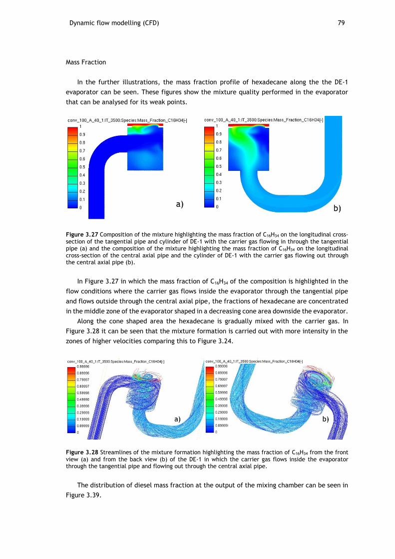
Dynamic flow modelling (CFD) 79
Mass Fraction
In the further illustrations, the mass fraction profile of hexadecane along the the DE-1
evaporator can be seen. These figures show the mixture quality performed in the evaporator
that can be analysed for its weak points.
Figure 3.27 Composition of the mixture highlighting the mass fraction of C16H34 on the longitudinal cross-section of the tangential pipe and cylinder of DE-1 with the carrier gas flowing in through the tangential pipe (a) and the composition of the mixture highlighting the mass fraction of C16H34 on the longitudinal cross-section of the central axial pipe and the cylinder of DE-1 with the carrier gas flowing out through the central axial pipe (b).
In Figure 3.27 in which the mass fraction of C16H34 of the composition is highlighted in the
flow conditions where the carrier gas flows inside the evaporator through the tangential pipe
and flows outside through the central axial pipe, the fractions of hexadecane are concentrated
in the middle zone of the evaporator shaped in a decreasing cone area downside the evaporator.
Along the cone shaped area the hexadecane is gradually mixed with the carrier gas. In
Figure 3.28 it can be seen that the mixture formation is carried out with more intensity in the
zones of higher velocities comparing this to Figure 3.24.
Figure 3.28 Streamlines of the mixture formation highlighting the mass fraction of C16H34 from the front view (a) and from the back view (b) of the DE-1 in which the carrier gas flows inside the evaporator through the tangential pipe and flowing out through the central axial pipe.
The distribution of diesel mass fraction at the output of the mixing chamber can be seen in
Figure 3.39.
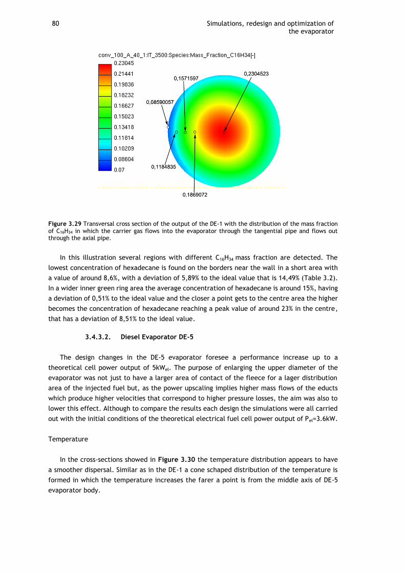
80 Simulations, redesign and optimization of the evaporator
Figure 3.29 Transversal cross section of the output of the DE-1 with the distribution of the mass fraction of C16H34 in which the carrier gas flows into the evaporator through the tangential pipe and flows out through the axial pipe.
In this illustration several regions with different C16H34 mass fraction are detected. The
lowest concentration of hexadecane is found on the borders near the wall in a short area with
a value of around 8,6%, with a deviation of 5,89% to the ideal value that is 14,49% (Table 3.2).
In a wider inner green ring area the average concentration of hexadecane is around 15%, having
a deviation of 0,51% to the ideal value and the closer a point gets to the centre area the higher
becomes the concentration of hexadecane reaching a peak value of around 23% in the centre,
that has a deviation of 8,51% to the ideal value.
3.4.3.2. Diesel Evaporator DE-5
The design changes in the DE-5 evaporator foresee a performance increase up to a
theoretical cell power output of 5kWel. The purpose of enlarging the upper diameter of the
evaporator was not just to have a larger area of contact of the fleece for a lager distribution
area of the injected fuel but, as the power upscaling implies higher mass flows of the educts
which produce higher velocities that correspond to higher pressure losses, the aim was also to
lower this effect. Although to compare the results each design the simulations were all carried
out with the initial conditions of the theoretical electrical fuel cell power output of Pel=3.6kW.
Temperature
In the cross-sections showed in Figure 3.30 the temperature distribution appears to have
a smoother dispersal. Similar as in the DE-1 a cone schaped distribution of the temperature is
formed in which the temperature increases the farer a point is from the middle axis of DE-5
evaporator body.
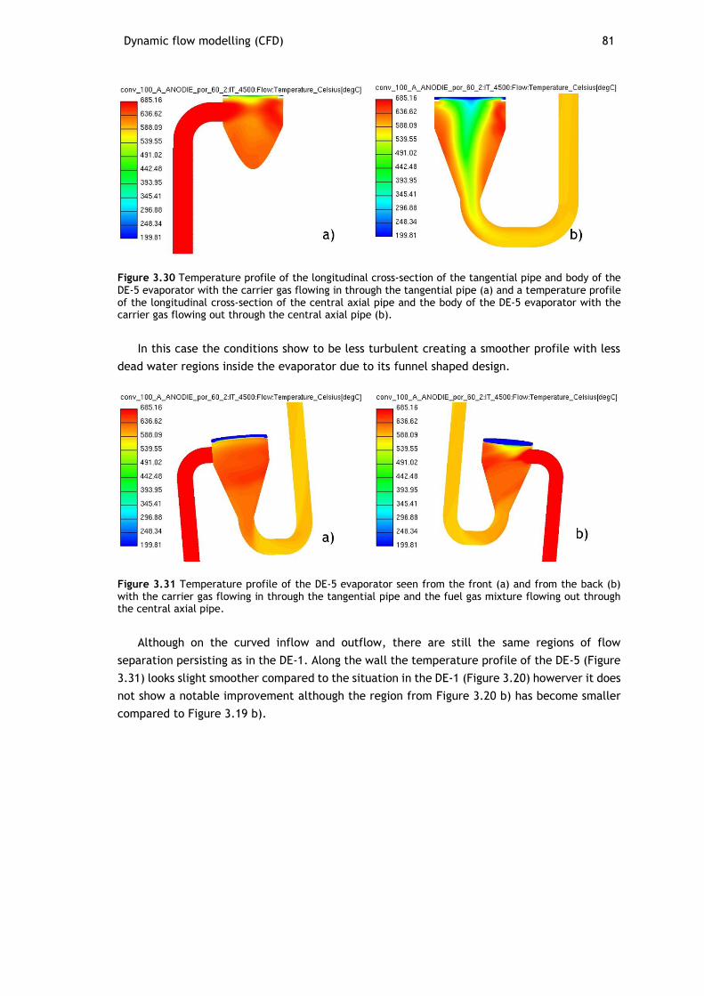
Dynamic flow modelling (CFD) 81
Figure 3.30 Temperature profile of the longitudinal cross-section of the tangential pipe and body of the DE-5 evaporator with the carrier gas flowing in through the tangential pipe (a) and a temperature profile of the longitudinal cross-section of the central axial pipe and the body of the DE-5 evaporator with the carrier gas flowing out through the central axial pipe (b).
In this case the conditions show to be less turbulent creating a smoother profile with less
dead water regions inside the evaporator due to its funnel shaped design.
Figure 3.31 Temperature profile of the DE-5 evaporator seen from the front (a) and from the back (b) with the carrier gas flowing in through the tangential pipe and the fuel gas mixture flowing out through the central axial pipe.
Although on the curved inflow and outflow, there are still the same regions of flow
separation persisting as in the DE-1. Along the wall the temperature profile of the DE-5 (Figure
3.31) looks slight smoother compared to the situation in the DE-1 (Figure 3.20) howerver it does
not show a notable improvement although the region from Figure 3.20 b) has become smaller
compared to Figure 3.19 b).
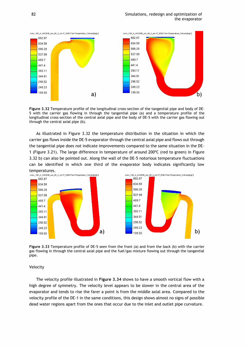
82 Simulations, redesign and optimization of the evaporator
Figure 3.32 Temperature profile of the longitudinal cross-section of the tangential pipe and body of DE-5 with the carrier gas flowing in through the tangential pipe (a) and a temperature profile of the longitudinal cross-section of the central axial pipe and the body of DE-5 with the carrier gas flowing out through the central axial pipe (b).
As illustrated in Figure 3.32 the temperature distribution in the situation in which the
carrier gas flows inside the DE-5 evaporator through the central axial pipe and flows out through
the tangential pipe does not indicate improvements compared to the same situation in the DE-
1 (Figure 3.21). The large difference in temperature of around 200ºC (red to green) in Figure
3.32 b) can also be pointed out. Along the wall of the DE-5 notorious temperature fluctuations
can be identified in which one third of the evaporator body indicates significantly low
temperatures.
Figure 3.33 Temperature profile of DE-5 seen from the front (a) and from the back (b) with the carrier gas flowing in through the central axial pipe and the fuel/gas mixture flowing out through the tangential pipe.
Velocity
The velocity profile illustrated in Figure 3.34 shows to have a smooth vortical flow with a
high degree of symmetry. The velocity level appears to be slower in the central area of the
evaporator and tends to rise the farer a point is from the middle axial area. Compared to the
velocity profile of the DE-1 in the same conditions, this design shows almost no signs of possible
dead water regions apart from the ones that occur due to the inlet and outlet pipe curvature.
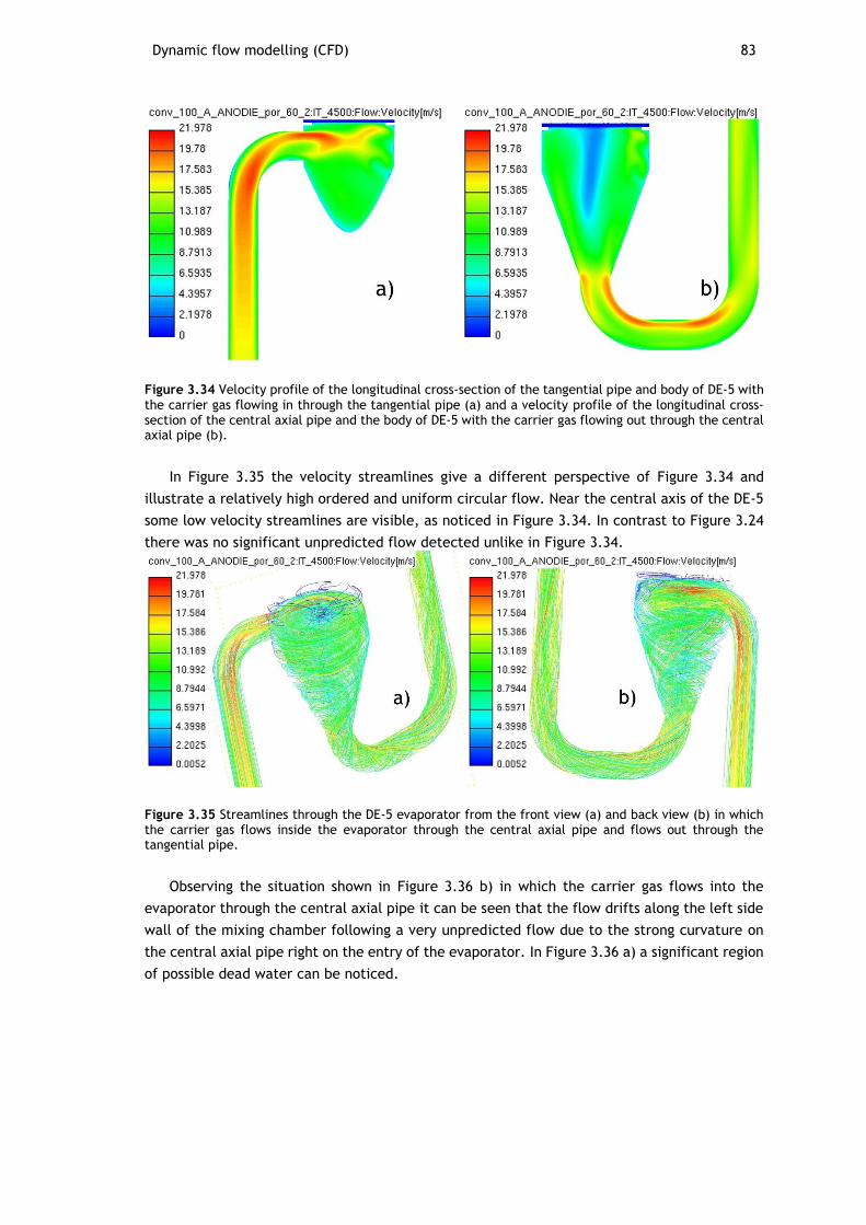
Dynamic flow modelling (CFD) 83
Figure 3.34 Velocity profile of the longitudinal cross-section of the tangential pipe and body of DE-5 with the carrier gas flowing in through the tangential pipe (a) and a velocity profile of the longitudinal cross-section of the central axial pipe and the body of DE-5 with the carrier gas flowing out through the central axial pipe (b).
In Figure 3.35 the velocity streamlines give a different perspective of Figure 3.34 and
illustrate a relatively high ordered and uniform circular flow. Near the central axis of the DE-5
some low velocity streamlines are visible, as noticed in Figure 3.34. In contrast to Figure 3.24
there was no significant unpredicted flow detected unlike in Figure 3.34.
Figure 3.35 Streamlines through the DE-5 evaporator from the front view (a) and back view (b) in which the carrier gas flows inside the evaporator through the central axial pipe and flows out through the tangential pipe.
Observing the situation shown in Figure 3.36 b) in which the carrier gas flows into the
evaporator through the central axial pipe it can be seen that the flow drifts along the left side
wall of the mixing chamber following a very unpredicted flow due to the strong curvature on
the central axial pipe right on the entry of the evaporator. In Figure 3.36 a) a significant region
of possible dead water can be noticed.
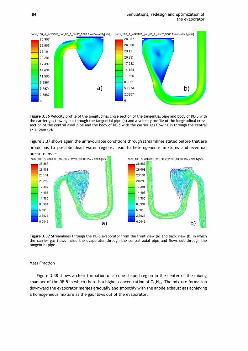
84 Simulations, redesign and optimization of the evaporator
Figure 3.36 Velocity profile of the longitudinal cross-section of the tangential pipe and body of DE-5 with the carrier gas flowing out through the tangential pipe (a) and a velocity profile of the longitudinal cross-section of the central axial pipe and the body of DE-5 with the carrier gas flowing in through the central axial pipe (b).
Figure 3.37 shows again the unfavourable conditions through streamlines stated before that are
propicious to possible dead water regions, lead to heterogeneous mixtures and eventual
pressure losses.
Figure 3.37 Streamlines through the DE-5 evaporator from the front view (a) and back view (b) in which the carrier gas flows inside the evaporator through the central axial pipe and flows out through the tangential pipe.
Mass Fraction
Figure 3.38 shows a clear formation of a cone shaped region in the center of the mixing
chamber of the DE-5 in which there is a higher concentration of C16H34. The mixture formation
downward the evaporator merges gradually and smoothly with the anode exhaust gas achieving
a homogeneous mixture as the gas flows out of the evaporator.
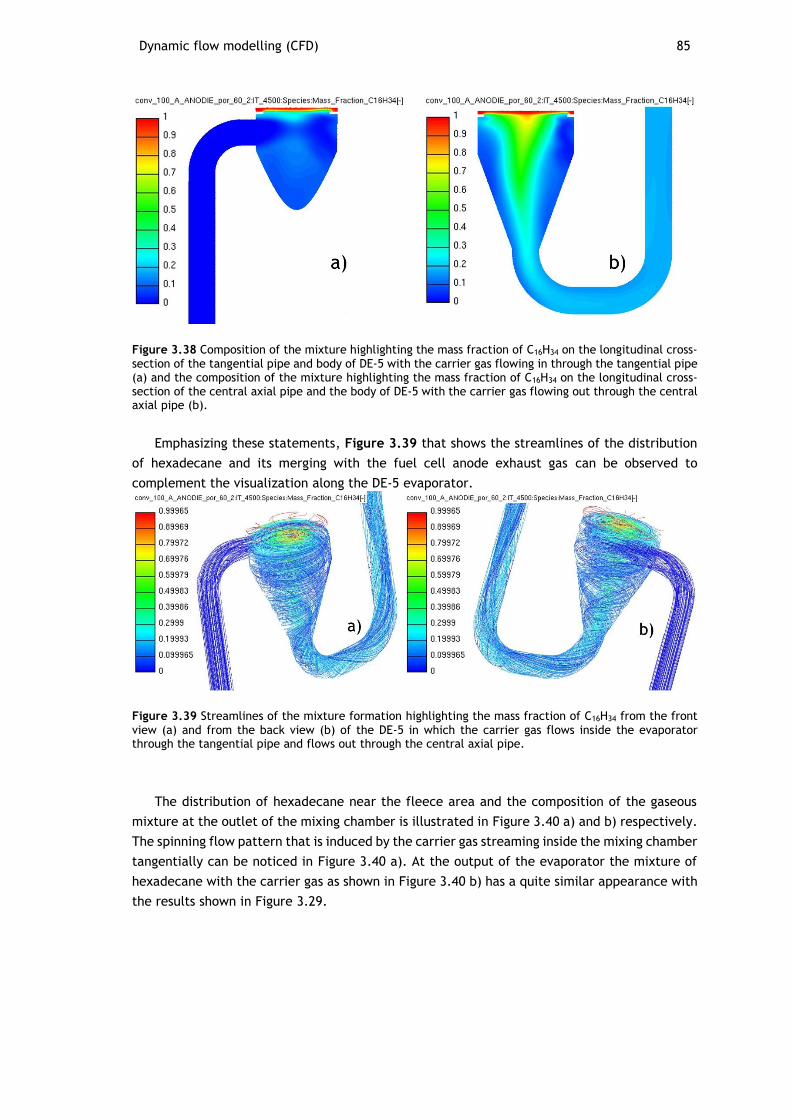
Dynamic flow modelling (CFD) 85
Figure 3.38 Composition of the mixture highlighting the mass fraction of C16H34 on the longitudinal cross-section of the tangential pipe and body of DE-5 with the carrier gas flowing in through the tangential pipe (a) and the composition of the mixture highlighting the mass fraction of C16H34 on the longitudinal cross-section of the central axial pipe and the body of DE-5 with the carrier gas flowing out through the central axial pipe (b).
Emphasizing these statements, Figure 3.39 that shows the streamlines of the distribution
of hexadecane and its merging with the fuel cell anode exhaust gas can be observed to
complement the visualization along the DE-5 evaporator.
Figure 3.39 Streamlines of the mixture formation highlighting the mass fraction of C16H34 from the front view (a) and from the back view (b) of the DE-5 in which the carrier gas flows inside the evaporator through the tangential pipe and flows out through the central axial pipe.
The distribution of hexadecane near the fleece area and the composition of the gaseous
mixture at the outlet of the mixing chamber is illustrated in Figure 3.40 a) and b) respectively.
The spinning flow pattern that is induced by the carrier gas streaming inside the mixing chamber
tangentially can be noticed in Figure 3.40 a). At the output of the evaporator the mixture of
hexadecane with the carrier gas as shown in Figure 3.40 b) has a quite similar appearance with
the results shown in Figure 3.29.
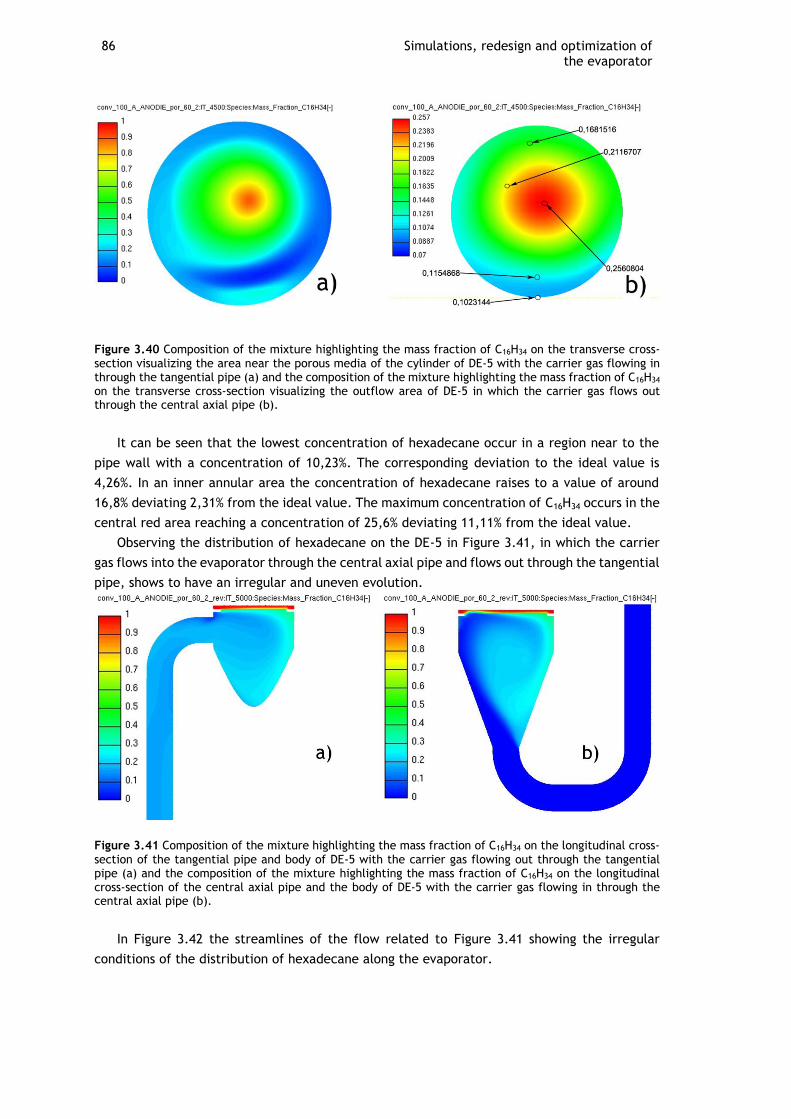
86 Simulations, redesign and optimization of the evaporator
Figure 3.40 Composition of the mixture highlighting the mass fraction of C16H34 on the transverse cross-section visualizing the area near the porous media of the cylinder of DE-5 with the carrier gas flowing in through the tangential pipe (a) and the composition of the mixture highlighting the mass fraction of C16H34 on the transverse cross-section visualizing the outflow area of DE-5 in which the carrier gas flows out through the central axial pipe (b).
It can be seen that the lowest concentration of hexadecane occur in a region near to the
pipe wall with a concentration of 10,23%. The corresponding deviation to the ideal value is
4,26%. In an inner annular area the concentration of hexadecane raises to a value of around
16,8% deviating 2,31% from the ideal value. The maximum concentration of C16H34 occurs in the
central red area reaching a concentration of 25,6% deviating 11,11% from the ideal value.
Observing the distribution of hexadecane on the DE-5 in Figure 3.41, in which the carrier
gas flows into the evaporator through the central axial pipe and flows out through the tangential
pipe, shows to have an irregular and uneven evolution.
Figure 3.41 Composition of the mixture highlighting the mass fraction of C16H34 on the longitudinal cross-section of the tangential pipe and body of DE-5 with the carrier gas flowing out through the tangential pipe (a) and the composition of the mixture highlighting the mass fraction of C16H34 on the longitudinal cross-section of the central axial pipe and the body of DE-5 with the carrier gas flowing in through the central axial pipe (b).
In Figure 3.42 the streamlines of the flow related to Figure 3.41 showing the irregular
conditions of the distribution of hexadecane along the evaporator.
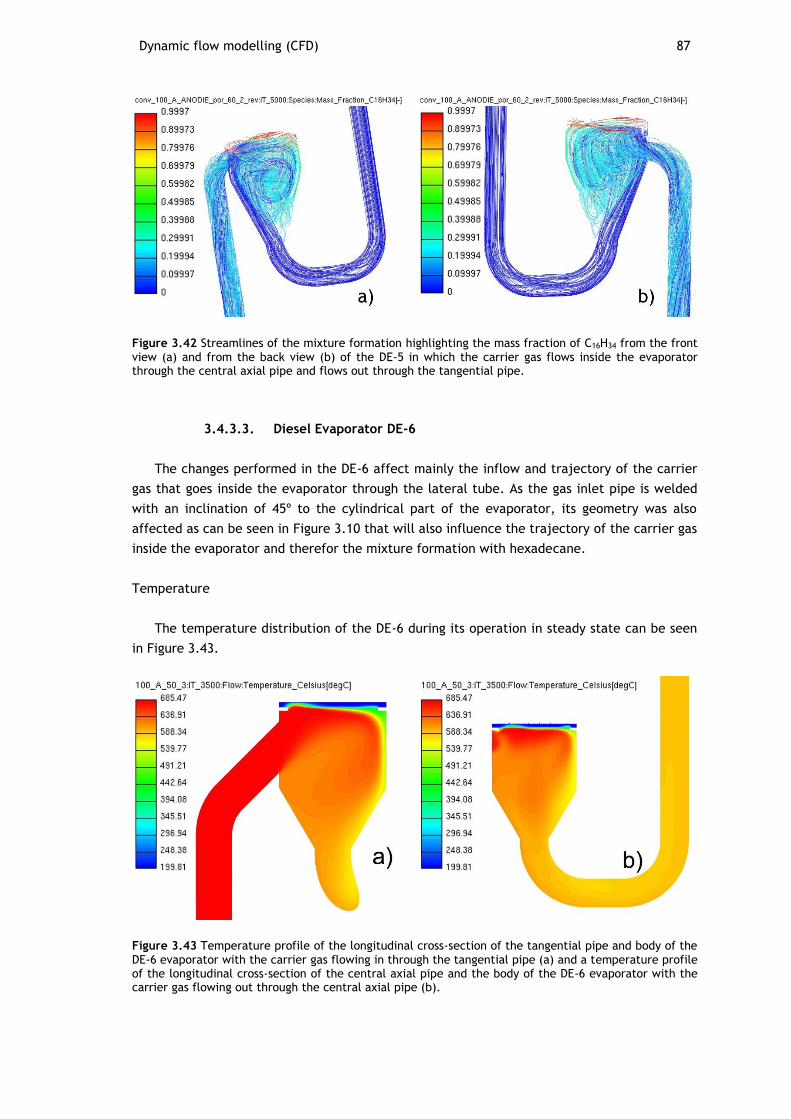
Dynamic flow modelling (CFD) 87
Figure 3.42 Streamlines of the mixture formation highlighting the mass fraction of C16H34 from the front view (a) and from the back view (b) of the DE-5 in which the carrier gas flows inside the evaporator through the central axial pipe and flows out through the tangential pipe.
3.4.3.3. Diesel Evaporator DE-6
The changes performed in the DE-6 affect mainly the inflow and trajectory of the carrier
gas that goes inside the evaporator through the lateral tube. As the gas inlet pipe is welded
with an inclination of 45º to the cylindrical part of the evaporator, its geometry was also
affected as can be seen in Figure 3.10 that will also influence the trajectory of the carrier gas
inside the evaporator and therefor the mixture formation with hexadecane.
Temperature
The temperature distribution of the DE-6 during its operation in steady state can be seen
in Figure 3.43.
Figure 3.43 Temperature profile of the longitudinal cross-section of the tangential pipe and body of the DE-6 evaporator with the carrier gas flowing in through the tangential pipe (a) and a temperature profile of the longitudinal cross-section of the central axial pipe and the body of the DE-6 evaporator with the carrier gas flowing out through the central axial pipe (b).
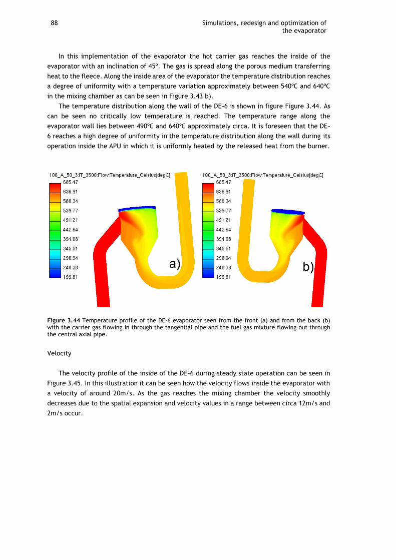
88 Simulations, redesign and optimization of the evaporator
In this implementation of the evaporator the hot carrier gas reaches the inside of the
evaporator with an inclination of 45º. The gas is spread along the porous medium transferring
heat to the fleece. Along the inside area of the evaporator the temperature distribution reaches
a degree of uniformity with a temperature variation approximately between 540ºC and 640ºC
in the mixing chamber as can be seen in Figure 3.43 b).
The temperature distribution along the wall of the DE-6 is shown in figure Figure 3.44. As
can be seen no critically low temperature is reached. The temperature range along the
evaporator wall lies between 490ºC and 640ºC approximately circa. It is foreseen that the DE-
6 reaches a high degree of uniformity in the temperature distribution along the wall during its
operation inside the APU in which it is uniformly heated by the released heat from the burner.
Figure 3.44 Temperature profile of the DE-6 evaporator seen from the front (a) and from the back (b) with the carrier gas flowing in through the tangential pipe and the fuel gas mixture flowing out through the central axial pipe.
Velocity
The velocity profile of the inside of the DE-6 during steady state operation can be seen in
Figure 3.45. In this illustration it can be seen how the velocity flows inside the evaporator with
a velocity of around 20m/s. As the gas reaches the mixing chamber the velocity smoothly
decreases due to the spatial expansion and velocity values in a range between circa 12m/s and
2m/s occur.
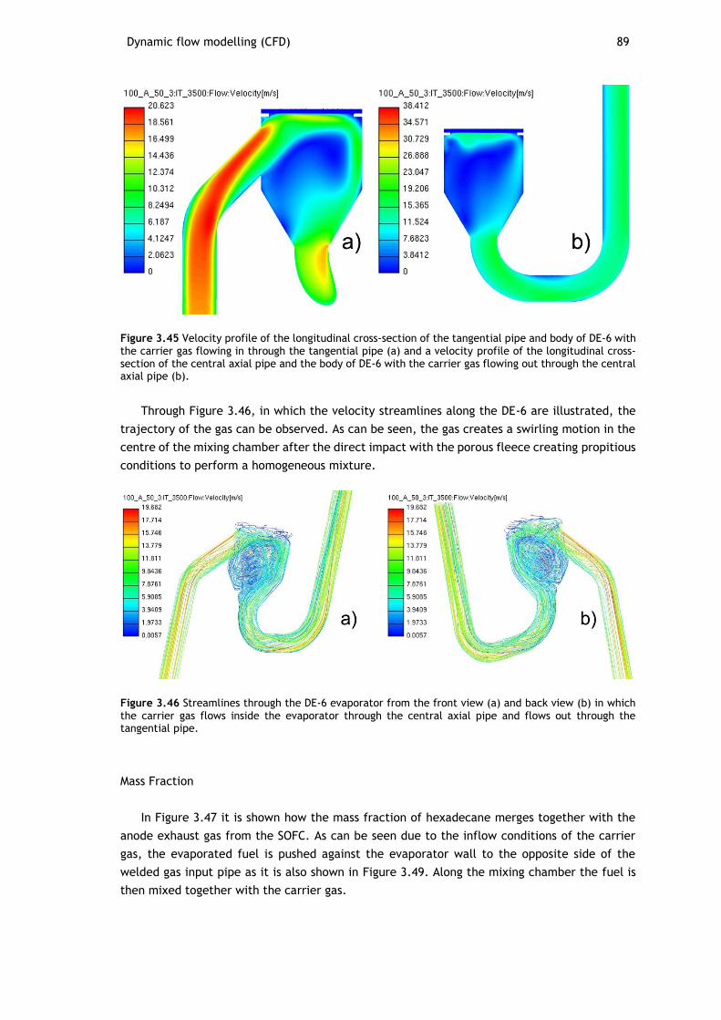
Dynamic flow modelling (CFD) 89
Figure 3.45 Velocity profile of the longitudinal cross-section of the tangential pipe and body of DE-6 with the carrier gas flowing in through the tangential pipe (a) and a velocity profile of the longitudinal cross-section of the central axial pipe and the body of DE-6 with the carrier gas flowing out through the central axial pipe (b).
Through Figure 3.46, in which the velocity streamlines along the DE-6 are illustrated, the
trajectory of the gas can be observed. As can be seen, the gas creates a swirling motion in the
centre of the mixing chamber after the direct impact with the porous fleece creating propitious
conditions to perform a homogeneous mixture.
Figure 3.46 Streamlines through the DE-6 evaporator from the front view (a) and back view (b) in which the carrier gas flows inside the evaporator through the central axial pipe and flows out through the tangential pipe.
Mass Fraction
In Figure 3.47 it is shown how the mass fraction of hexadecane merges together with the
anode exhaust gas from the SOFC. As can be seen due to the inflow conditions of the carrier
gas, the evaporated fuel is pushed against the evaporator wall to the opposite side of the
welded gas input pipe as it is also shown in Figure 3.49. Along the mixing chamber the fuel is
then mixed together with the carrier gas.
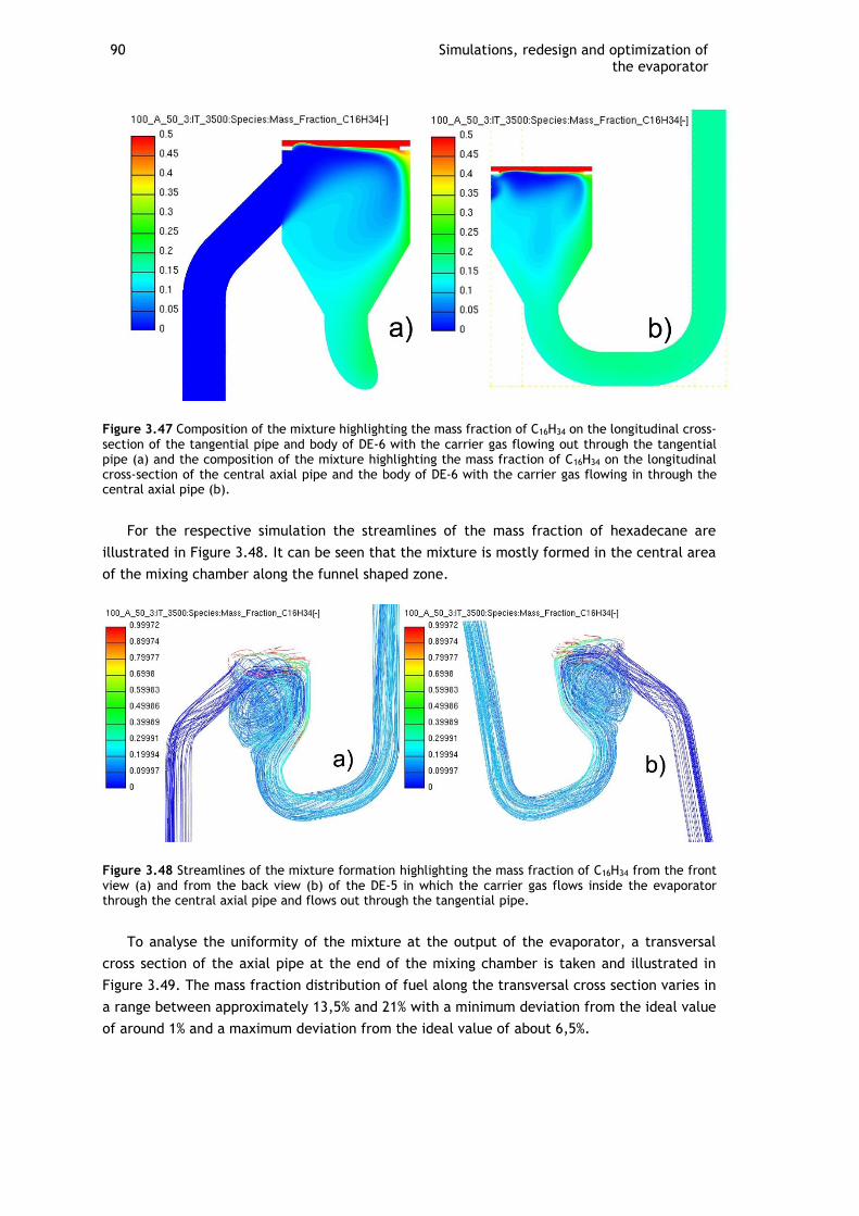
90 Simulations, redesign and optimization of the evaporator
Figure 3.47 Composition of the mixture highlighting the mass fraction of C16H34 on the longitudinal cross-section of the tangential pipe and body of DE-6 with the carrier gas flowing out through the tangential pipe (a) and the composition of the mixture highlighting the mass fraction of C16H34 on the longitudinal cross-section of the central axial pipe and the body of DE-6 with the carrier gas flowing in through the central axial pipe (b).
For the respective simulation the streamlines of the mass fraction of hexadecane are
illustrated in Figure 3.48. It can be seen that the mixture is mostly formed in the central area
of the mixing chamber along the funnel shaped zone.
Figure 3.48 Streamlines of the mixture formation highlighting the mass fraction of C16H34 from the front view (a) and from the back view (b) of the DE-5 in which the carrier gas flows inside the evaporator through the central axial pipe and flows out through the tangential pipe.
To analyse the uniformity of the mixture at the output of the evaporator, a transversal
cross section of the axial pipe at the end of the mixing chamber is taken and illustrated in
Figure 3.49. The mass fraction distribution of fuel along the transversal cross section varies in
a range between approximately 13,5% and 21% with a minimum deviation from the ideal value
of around 1% and a maximum deviation from the ideal value of about 6,5%.
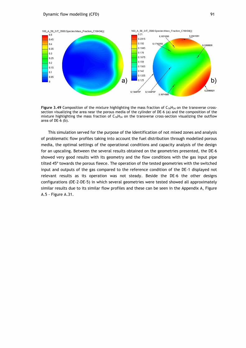
Dynamic flow modelling (CFD) 91
Figure 3.49 Composition of the mixture highlighting the mass fraction of C16H34 on the transverse cross-section visualizing the area near the porous media of the cylinder of DE-6 (a) and the composition of the mixture highlighting the mass fraction of C16H34 on the transverse cross-section visualizing the outflow area of DE-6 (b).
This simulation served for the purpose of the Identification of not mixed zones and analysis
of problematic flow profiles taking into account the fuel distribution through modelled porous
media, the optimal settings of the operational conditions and capacity analysis of the design
for an upscaling. Between the several results obtained on the geometries presented, the DE-6
showed very good results with its geometry and the flow conditions with the gas input pipe
tilted 45º towards the porous fleece. The operation of the tested geometries with the switched
input and outputs of the gas compared to the reference condition of the DE-1 displayed not
relevant results as its operation was not steady. Beside the DE-6 the other designs
configurations (DE-2-DE-5) in which several geometries were tested showed all approximately
similar results due to its similar flow profiles and these can be seen in the Appendix A, Figure
A.5 - Figure A.31.

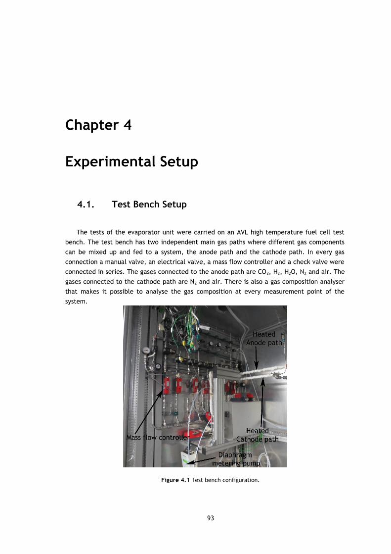
93
Chapter 4
Experimental Setup
4.1. Test Bench Setup
The tests of the evaporator unit were carried on an AVL high temperature fuel cell test
bench. The test bench has two independent main gas paths where different gas components
can be mixed up and fed to a system, the anode path and the cathode path. In every gas
connection a manual valve, an electrical valve, a mass flow controller and a check valve were
connected in series. The gases connected to the anode path are CO2, H2, H2O, N2 and air. The
gases connected to the cathode path are N2 and air. There is also a gas composition analyser
that makes it possible to analyse the gas composition at every measurement point of the
system.
Figure 4.1 Test bench configuration.
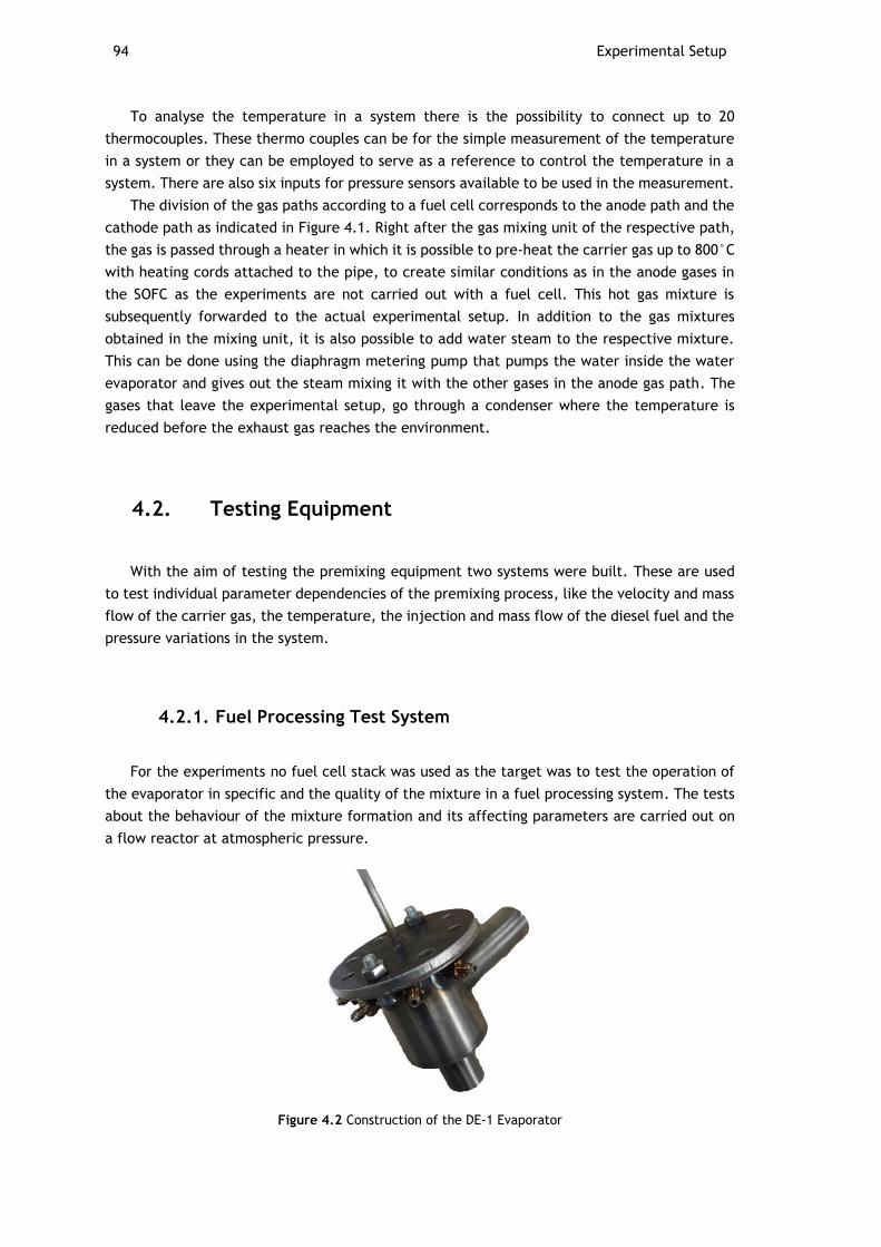
94 Experimental Setup
To analyse the temperature in a system there is the possibility to connect up to 20
thermocouples. These thermo couples can be for the simple measurement of the temperature
in a system or they can be employed to serve as a reference to control the temperature in a
system. There are also six inputs for pressure sensors available to be used in the measurement.
The division of the gas paths according to a fuel cell corresponds to the anode path and the
cathode path as indicated in Figure 4.1. Right after the gas mixing unit of the respective path,
the gas is passed through a heater in which it is possible to pre-heat the carrier gas up to 800°C
with heating cords attached to the pipe, to create similar conditions as in the anode gases in
the SOFC as the experiments are not carried out with a fuel cell. This hot gas mixture is
subsequently forwarded to the actual experimental setup. In addition to the gas mixtures
obtained in the mixing unit, it is also possible to add water steam to the respective mixture.
This can be done using the diaphragm metering pump that pumps the water inside the water
evaporator and gives out the steam mixing it with the other gases in the anode gas path. The
gases that leave the experimental setup, go through a condenser where the temperature is
reduced before the exhaust gas reaches the environment.
4.2. Testing Equipment
With the aim of testing the premixing equipment two systems were built. These are used
to test individual parameter dependencies of the premixing process, like the velocity and mass
flow of the carrier gas, the temperature, the injection and mass flow of the diesel fuel and the
pressure variations in the system.
4.2.1. Fuel Processing Test System
For the experiments no fuel cell stack was used as the target was to test the operation of
the evaporator in specific and the quality of the mixture in a fuel processing system. The tests
about the behaviour of the mixture formation and its affecting parameters are carried out on
a flow reactor at atmospheric pressure.
Figure 4.2 Construction of the DE-1 Evaporator
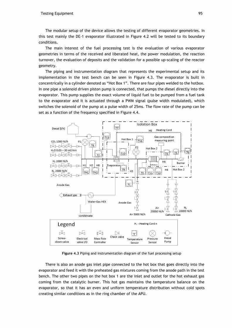
Testing Equipment 95
The modular setup of the device allows the testing of different evaporator geometries. In
this test mainly the DE-1 evaporator illustrated in Figure 4.2 will be tested to its boundary
conditions.
The main interest of the fuel processing test is the evaluation of various evaporator
geometries in terms of the received and liberated heat, the power modulation, the reaction
turnover, the evaluation of deposits and the validation for a possible up-scaling of the reactor
geometry.
The piping and instrumentation diagram that represents the experimental setup and its
implementation in the test bench can be seen in Figure 4.3. The evaporator is built in
concentrically in a cylinder denoted as “Hot Box 1”. There are four pipes welded to the hotbox.
In one pipe a solenoid driven piston pump is connected, that pumps the diesel directly into the
evaporator. This pump supplies the exact volume of liquid fuel to be pumped from a fuel tank
to the evaporator and it is actuated through a PWM signal (pulse width modulated), which
switches the solenoid of the pump at a pulse width of 25ms. The flow rate of the pump can be
set as a function of the frequency specified in Figure 4.4.
Figure 4.3 Piping and instrumentation diagram of the fuel processing setup
There is also an anode gas inlet pipe connected to the hot box that goes directly into the
evaporator and feed it with the preheated gas mixtures coming from the anode path in the test
bench. The other two pipes on the hot box 1 are the inlet and outlet for the hot exhaust gas
coming from the catalytic burner. This hot gas maintains the temperature balance on the
evaporator, so that it has an even and uniform temperature distribution without cold spots
creating similar conditions as in the ring chamber of the APU.
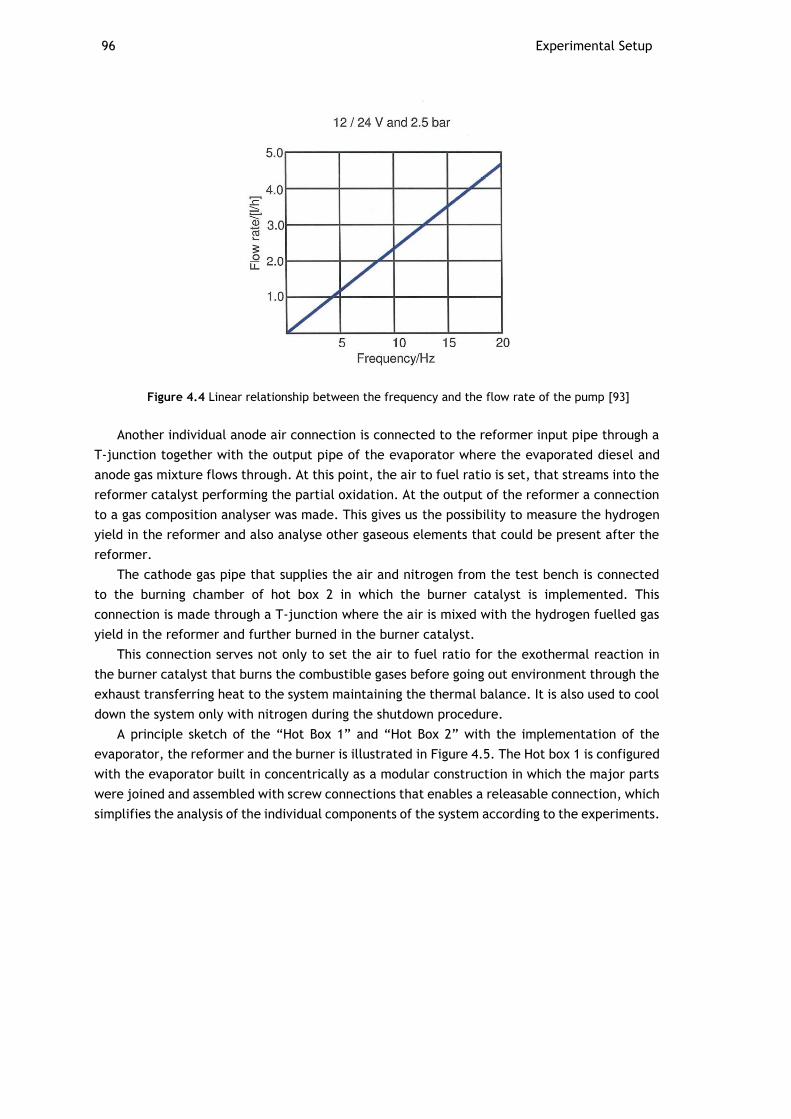
96 Experimental Setup
Figure 4.4 Linear relationship between the frequency and the flow rate of the pump [93]
Another individual anode air connection is connected to the reformer input pipe through a
T-junction together with the output pipe of the evaporator where the evaporated diesel and
anode gas mixture flows through. At this point, the air to fuel ratio is set, that streams into the
reformer catalyst performing the partial oxidation. At the output of the reformer a connection
to a gas composition analyser was made. This gives us the possibility to measure the hydrogen
yield in the reformer and also analyse other gaseous elements that could be present after the
reformer.
The cathode gas pipe that supplies the air and nitrogen from the test bench is connected
to the burning chamber of hot box 2 in which the burner catalyst is implemented. This
connection is made through a T-junction where the air is mixed with the hydrogen fuelled gas
yield in the reformer and further burned in the burner catalyst.
This connection serves not only to set the air to fuel ratio for the exothermal reaction in
the burner catalyst that burns the combustible gases before going out environment through the
exhaust transferring heat to the system maintaining the thermal balance. It is also used to cool
down the system only with nitrogen during the shutdown procedure.
A principle sketch of the “Hot Box 1” and “Hot Box 2” with the implementation of the
evaporator, the reformer and the burner is illustrated in Figure 4.5. The Hot box 1 is configured
with the evaporator built in concentrically as a modular construction in which the major parts
were joined and assembled with screw connections that enables a releasable connection, which
simplifies the analysis of the individual components of the system according to the experiments.
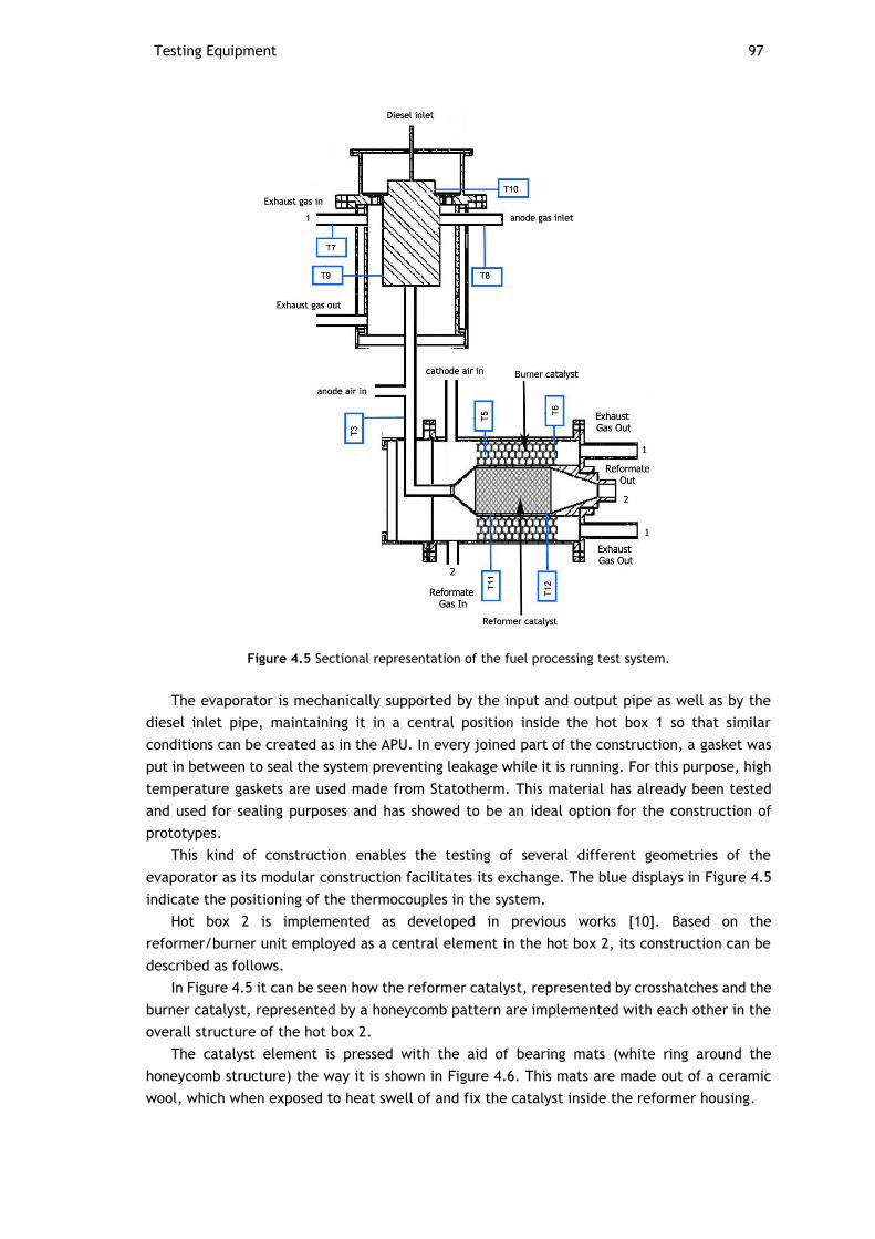
Testing Equipment 97
Figure 4.5 Sectional representation of the fuel processing test system.
The evaporator is mechanically supported by the input and output pipe as well as by the
diesel inlet pipe, maintaining it in a central position inside the hot box 1 so that similar
conditions can be created as in the APU. In every joined part of the construction, a gasket was
put in between to seal the system preventing leakage while it is running. For this purpose, high
temperature gaskets are used made from Statotherm. This material has already been tested
and used for sealing purposes and has showed to be an ideal option for the construction of
prototypes.
This kind of construction enables the testing of several different geometries of the
evaporator as its modular construction facilitates its exchange. The blue displays in Figure 4.5
indicate the positioning of the thermocouples in the system.
Hot box 2 is implemented as developed in previous works [10]. Based on the
reformer/burner unit employed as a central element in the hot box 2, its construction can be
described as follows.
In Figure 4.5 it can be seen how the reformer catalyst, represented by crosshatches and the
burner catalyst, represented by a honeycomb pattern are implemented with each other in the
overall structure of the hot box 2.
The catalyst element is pressed with the aid of bearing mats (white ring around the
honeycomb structure) the way it is shown in Figure 4.6. This mats are made out of a ceramic
wool, which when exposed to heat swell of and fix the catalyst inside the reformer housing.
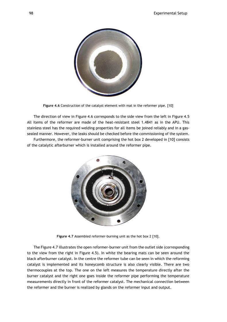
98 Experimental Setup
Figure 4.6 Construction of the catalyst element with mat in the reformer pipe. [10]
The direction of view in Figure 4.6 corresponds to the side view from the left in Figure 4.5
All items of the reformer are made of the heat-resistant steel 1.4841 as in the APU. This
stainless steel has the required welding properties for all items be joined reliably and in a gas-
sealed manner. However, the leaks should be checked before the commissioning of the system.
Furthermore, the reformer-burner unit comprising the hot box 2 developed in [10] consists
of the catalytic afterburner which is installed around the reformer pipe.
Figure 4.7 Assembled reformer-burning unit as the hot box 2 [10].
The Figure 4.7 illustrates the open reformer-burner unit from the outlet side (corresponding
to the view from the right in Figure 4.5). In white the bearing mats can be seen around the
black afterburner catalyst. In the centre the reformer tube can be seen in which the reforming
catalyst is implemented and its honeycomb structure is also clearly visible. There are two
thermocouples at the top. The one on the left measures the temperature directly after the
burner catalyst and the right one goes inside the reformer pipe performing the temperature
measurements directly in front of the reformer catalyst. The mechanical connection between
the reformer and the burner is realized by glands on the reformer input and output.
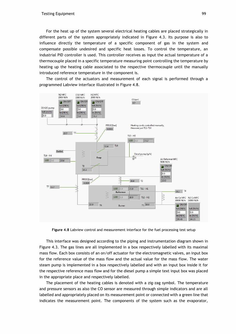
Testing Equipment 99
For the heat up of the system several electrical heating cables are placed strategically in
different parts of the system appropriately indicated in Figure 4.3. Its purpose is also to
influence directly the temperature of a specific component of gas in the system and
compensate possible undesired and specific heat losses. To control the temperature, an
industrial PID controller is used. This controller receives as input the actual temperature of a
thermocouple placed in a specific temperature measuring point controlling the temperature by
heating up the heating cable associated to the respective thermocouple until the manually
introduced reference temperature in the component is.
The control of the actuators and measurement of each signal is performed through a
programmed Labview interface illustrated in Figure 4.8.
Figure 4.8 Labview control and measurement interface for the fuel processing test setup
This interface was designed according to the piping and instrumentation diagram shown in
Figure 4.3. The gas lines are all implemented in a box respectively labelled with its maximal
mass flow. Each box consists of an on/off actuator for the electromagnetic valves, an input box
for the reference value of the mass flow and the actual value for the mass flow. The water
steam pump is implemented in a box respectively labelled and with an input box inside it for
the respective reference mass flow and for the diesel pump a simple text input box was placed
in the appropriate place and respectively labelled.
The placement of the heating cables is denoted with a zig-zag symbol. The temperature
and pressure sensors as also the CO sensor are measured through simple indicators and are all
labelled and appropriately placed on its measurement point or connected with a green line that
indicates the measurement point. The components of the system such as the evaporator,
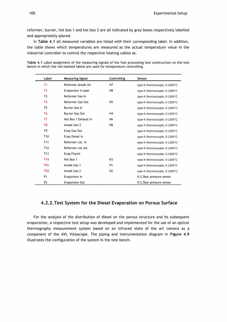
100 Experimental Setup
reformer, burner, hot box 1 and hot box 2 are all indicated by grey boxes respectively labelled
and appropriately placed.
In Table 4.1 all measured variables are listed with their corresponding label. In addition,
the table shows which temperatures are measured as the actual temperature value in the
industrial controller to control the respective heating cables as.
Table 4.1 Label assignment of the measuring signals of the fuel processing test construction on the test bench in which the red marked labels are used for temperature controlling.
Label Measuring Signal Controlling Sensor
T1 Reformer Anode Air H7 type-K thermocouple, 0-1300°C
T2 Evaporator in pipe H8 type-K thermocouple, 0-1300°C
T3 Reformer Gas In type-K thermocouple, 0-1300°C
T4 Reformer Gas Out H5 type-K thermocouple, 0-1300°C
T5 Burner Gas In type-K thermocouple, 0-1300°C
T6 Burner Gas Out H4 type-K thermocouple, 0-1300°C
T7 Hot Box 1 Exhaust In H6 type-K thermocouple, 0-1300°C
T8 Anode Gas 3 H8 type-K thermocouple, 0-1300°C
T9 Evap Gas Out type-K thermocouple, 0-1300°C
T10 Evap Diesel In type-K thermocouple, 0-1300°C
T11 Reformer cat. In type-K thermocouple, 0-1300°C
T12 Reformer cat out type-K thermocouple, 0-1300°C
T13 Evap Flanch type-K thermocouple, 0-1300°C
T14 Hot Box 1 H3 type-K thermocouple, 0-1300°C
TH1 Anode Gas 1 H1 type-K thermocouple, 0-1300°C
TH2 Anode Gas 2 H2 type-K thermocouple, 0-1300°C
P1 Evaporator In 0-2,5bar pressure sensor
P2 Evaporator Out 0-2,5bar pressure sensor
4.2.2. Test System for the Diesel Evaporation on Porous Surface
For the analysis of the distribution of diesel on the porous structure and its subsequent
evaporation, a respective test setup was developed and implemented for the use of an optical
thermography measurement system based on an infrared state of the art camera as a
component of the AVL Visioscope. The piping and instrumentation diagram in Figure 4.9
illustrates the configuration of the system in the test bench.
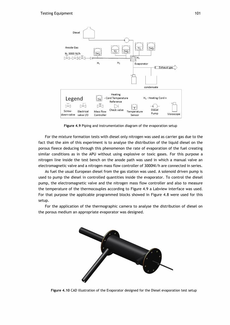
Testing Equipment 101
Figure 4.9 Piping and instrumentation diagram of the evaporation setup
For the mixture formation tests with diesel only nitrogen was used as carrier gas due to the
fact that the aim of this experiment is to analyse the distribution of the liquid diesel on the
porous fleece deducing through this phenomenon the rate of evaporation of the fuel creating
similar conditions as in the APU without using explosive or toxic gases. For this purpose a
nitrogen line inside the test bench on the anode path was used in which a manual valve an
electromagnetic valve and a nitrogen mass flow controller of 3000Nl/h are connected in series.
As fuel the usual European diesel from the gas station was used. A solenoid driven pump is
used to pump the diesel in controlled quantities inside the evaporator. To control the diesel
pump, the electromagnetic valve and the nitrogen mass flow controller and also to measure
the temperature of the thermocouples according to Figure 4.9 a Labview interface was used.
For that purpose the applicable programmed blocks showed in Figure 4.8 were used for this
setup.
For the application of the thermographic camera to analyse the distribution of diesel on
the porous medium an appropriate evaporator was designed.
Figure 4.10 CAD illustration of the Evaporator designed for the Diesel evaporation test setup
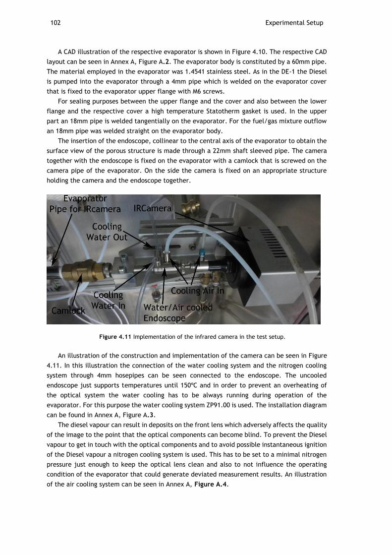
102 Experimental Setup
A CAD illustration of the respective evaporator is shown in Figure 4.10. The respective CAD
layout can be seen in Annex A, Figure A.2. The evaporator body is constituted by a 60mm pipe.
The material employed in the evaporator was 1.4541 stainless steel. As in the DE-1 the Diesel
is pumped into the evaporator through a 4mm pipe which is welded on the evaporator cover
that is fixed to the evaporator upper flange with M6 screws.
For sealing purposes between the upper flange and the cover and also between the lower
flange and the respective cover a high temperature Statotherm gasket is used. In the upper
part an 18mm pipe is welded tangentially on the evaporator. For the fuel/gas mixture outflow
an 18mm pipe was welded straight on the evaporator body.
The insertion of the endoscope, collinear to the central axis of the evaporator to obtain the
surface view of the porous structure is made through a 22mm shaft sleeved pipe. The camera
together with the endoscope is fixed on the evaporator with a camlock that is screwed on the
camera pipe of the evaporator. On the side the camera is fixed on an appropriate structure
holding the camera and the endoscope together.
Figure 4.11 Implementation of the infrared camera in the test setup.
An illustration of the construction and implementation of the camera can be seen in Figure
4.11. In this illustration the connection of the water cooling system and the nitrogen cooling
system through 4mm hosepipes can be seen connected to the endoscope. The uncooled
endoscope just supports temperatures until 150ºC and in order to prevent an overheating of
the optical system the water cooling has to be always running during operation of the
evaporator. For this purpose the water cooling system ZP91.00 is used. The installation diagram
can be found in Annex A, Figure A.3.
The diesel vapour can result in deposits on the front lens which adversely affects the quality
of the image to the point that the optical components can become blind. To prevent the Diesel
vapour to get in touch with the optical components and to avoid possible instantaneous ignition
of the Diesel vapour a nitrogen cooling system is used. This has to be set to a minimal nitrogen
pressure just enough to keep the optical lens clean and also to not influence the operating
condition of the evaporator that could generate deviated measurement results. An illustration
of the air cooling system can be seen in Annex A, Figure A.4.
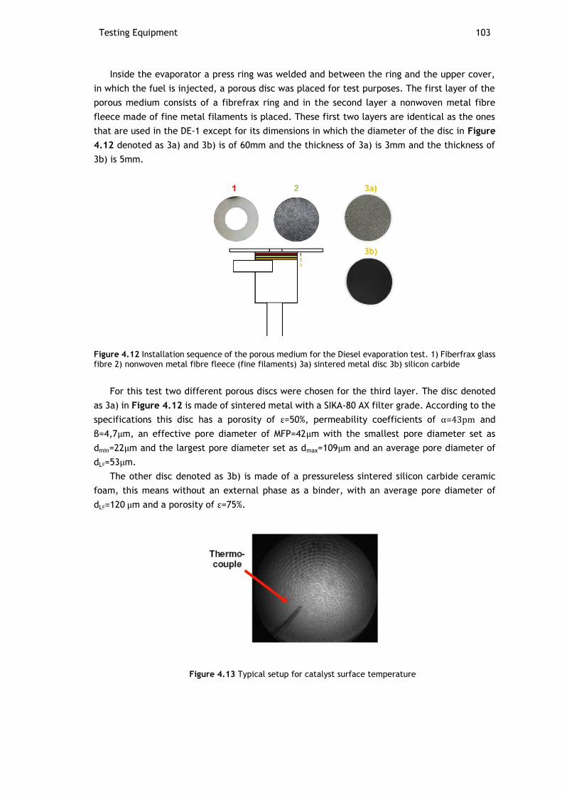
Testing Equipment 103
Inside the evaporator a press ring was welded and between the ring and the upper cover,
in which the fuel is injected, a porous disc was placed for test purposes. The first layer of the
porous medium consists of a fibrefrax ring and in the second layer a nonwoven metal fibre
fleece made of fine metal filaments is placed. These first two layers are identical as the ones
that are used in the DE-1 except for its dimensions in which the diameter of the disc in Figure
4.12 denoted as 3a) and 3b) is of 60mm and the thickness of 3a) is 3mm and the thickness of
3b) is 5mm.
Figure 4.12 Installation sequence of the porous medium for the Diesel evaporation test. 1) Fiberfrax glass fibre 2) nonwoven metal fibre fleece (fine filaments) 3a) sintered metal disc 3b) silicon carbide
For this test two different porous discs were chosen for the third layer. The disc denoted
as 3a) in Figure 4.12 is made of sintered metal with a SIKA-80 AX filter grade. According to the
specifications this disc has a porosity of ε=50%, permeability coefficients of α=43pm and
β=4,7μm, an effective pore diameter of MFP=42μm with the smallest pore diameter set as
dmin=22μm and the largest pore diameter set as dmax=109μm and an average pore diameter of
dLε=53μm.
The other disc denoted as 3b) is made of a pressureless sintered silicon carbide ceramic
foam, this means without an external phase as a binder, with an average pore diameter of
dLε=120 μm and a porosity of ε=75%.
Figure 4.13 Typical setup for catalyst surface temperature
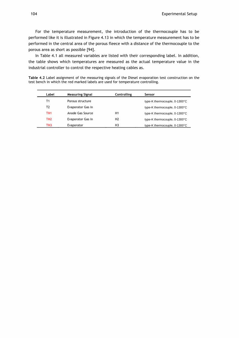
104 Experimental Setup
For the temperature measurement, the introduction of the thermocouple has to be
performed like it is illustrated in Figure 4.13 in which the temperature measurement has to be
performed in the central area of the porous fleece with a distance of the thermocouple to the
porous area as short as possible [94].
In Table 4.1 all measured variables are listed with their corresponding label. In addition,
the table shows which temperatures are measured as the actual temperature value in the
industrial controller to control the respective heating cables as.
Table 4.2 Label assignment of the measuring signals of the Diesel evaporation test construction on the test bench in which the red marked labels are used for temperature controlling.
Label Measuring Signal Controlling Sensor
T1 Porous structure type-K thermocouple, 0-1300°C
T2 Evaporator Gas in type-K thermocouple, 0-1300°C
TH1 Anode Gas Source H1 type-K thermocouple, 0-1300°C
TH2 Evaporator Gas in H2 type-K thermocouple, 0-1300°C
TH3 Evaporator H3 type-K thermocouple, 0-1300°C
105
Chapter 5
Practical Implementation and Evaluation
For the tests performed on the evaporator unit, a test program is designed. In it, all the
procedures and requirements for the commissioning of the tests are described. At first all the
components are tested, calibrated and put into operation individually. Further the modules
corresponding to the system are assembled together and put into operation as a unit.
5.1. Commissioning of the Fuel processing Test System
Before all the modules are assembled together they have to be checked for leakage as
there are burning and poisoning gases in the system and to guarantee the proper mass flow of
the substances to ensure the desired reactions. For this purpose the output is sealed with a
blanking plug and the anode air is pumped into the module until a pressure of 1,5 bar is
created inside it. In this state, all welds and fittings are wetted with soapy leak spray, which
detects leaks noticeable through a soapy blistering.
After the structures are completely isolated, they are assembled and the system must be
heated initially for 6 hours at a temperature of 500°C before the first test so that the glass
fibre mats, with which the catalysts elements and the porous disc are pressed, swell up and
ensure a tight fit. After this process, the tests can be performed on the test setup.
Before the diesel pump is used, it has to be calibrated for the diesel fuel that is used for
this application. The diesel pump is actuated through a PWM (pulse width modulation) signal.
From the datasheet the relation of diesel with the respective frequency (Figure 4.4) and the
on-time can be extracted.
Knowing that the on-time of the pump is Ton=0,025s and the frequency, f, is the inverse of
the on-time and off-time, Toff, the following relations are used to set the mass flow of diesel
for the pump in Labview:
𝑇𝑜𝑓𝑓 =1
𝑓− 𝑇𝑜𝑛 (5.1)
The relationship between the volume flow rate of the pump, �̇�𝑝 and the frequency is given
by:
106 Practical Implementation and Evaluation
𝑓 =�̇�𝑝
𝑐1
(5.2)
The factor, c1=10/2,3, is the relational factor between diesel and the volume flow rate of
the pump and can be extracted from [93]. Substituting (5.2) in (5.1) the following equation
can be derived:
𝑇𝑜𝑓𝑓 =𝑐1
�̇�𝑝
− 𝑇𝑜𝑛 (5.3)
Through the approximation that one litre of water at 20ºC and at atmosphere pressure is
equivalent to one kilogram, the coefficient c1 can simply be multiplied by 1000 [h/g] and as
the diesel can be obtained through a correction factor, c2, multiplied by the mass flow of the
pump �̇�𝑝 obtaining the following expression:
𝑇𝑜𝑓𝑓 =230
�̇�𝑑 × 𝑐2
− 0,025 (5.4)
To determine the correction factor c2, diesel fuel was pumped to a canister for one hour
with a mass flow of 300g/h. The mass difference of the canister, that is, the mass of diesel
after one hour was divided by the reference mass flow of 300g/h obtaining the correction
factor c2.
5.1.1. Heat up Procedures
Before starting the tests, the system has to be heated up with the installed heating cables.
The aim is to reach operating temperature in all components of the experimental setup, that
means in the specific case that it has to be achieved a temperature of T10=500ºC on the porous
structure, T6=600ºC on the reformer catalyst output and T12=600ºC on the afterburner catalyst
output. The heating cords are set up with the appropriate reference temperature to heat up
the system. With these temperatures it is possible to start the operation of the system.
In order to achieve a uniform and slow heating of the catalysts, the porous structure and
the mixing chamber of the evaporator a volume flow of 750Nl/h is set in the anode path and
cathode path for air and nitrogen.
5.1.2. Operational Procedures
After reaching the desired conditions in the system, the input parameters for the operation
can be set to start up the system. For the start-up sequence first the water steam is set on the
anode path according to the desired operation point. Subsequently it is necessary to wait a
short time interval until the temperature stabilizes. In a next step, the cathode air is set for
the afterburner according to the pretended operation point. In a further step the pretended
nitrogen volume flow is introduced, setting right after the respective diesel mass flow. After
these settings the anode air in the reformer has to be regulated according to the introduced
Commissioning of the Fuel processing Test System 107
diesel. Usually for this purpose an air to fuel ratio of approximately 0,36 is established so that
the output temperature results in a value of about 770ºC. If necessary the burner air has to be
regulated so that it maintains a temperature around 850ºC. This happens at an air to fuel ratio
of about 4,8. As the reformer is operated in a sub stoichiometric mode this is in the process of
regulating the temperature of the reformer, to raise the temperature, the air to fuel ratio is
increased up this means that the air on the reformer input has to be increased. To lower the
temperature in a sub stoichiometric burning mode the inverse process is performed.
The afterburner is operated in a lean burning mode, so the process of regulating the
temperature is inversed compared to the sub stoichiometric burning. This means that during
the process of adjusting the temperature in the burner, to lower the temperature the air to
fuel ratio is increased, in consequence the temperature in the afterburner is reduced. To
increase the temperature in the afterburner the process is inversed. After the start-up of the
fuel processing system the heating cords can be turned off. In order to keep a temperature
balance of the system the exothermic reactions performed in the reformer and in the
afterburner are used.
For the operation of the fuel processing system to perform the proof of concept of the DE-
1 the following operation points were set in the following order.
Table 5.1 Input parameter configuration for tests with different load points
Pel Ca. Air [Nl/h] H2O [g/h] An.N2 [Nl/h] Diesel [g/h] An. Air [Nl/h]
735W 5750 94 467,3 174,09 666
843W 6594 107,78 535,866 200 763,72
1470W 11000 245,12 727,65 331,34 1270
2205W 15400 411,48 1162 471,6 1785
In every transition from one load point to another the same procedure used to start up the
system is repeated regulating the temperature of the reformer and afterburner as mentioned
to a temperature value of about 770ºC in the reformer output and a burner output value of
around 850ºC. According to the heat losses of the system the temperature value in the burner
can also be slightly increased just enough to not overheat the steel and to feed the evaporator
with the amount of heat required to overcome the latent heat of vaporization of diesel and so
perform its transition of phase.
5.1.3. Test Results
The operational input and output parameters of the DE-1 evaporator during the tests are
illustrated in Figure 5.1. The different operational points can be determined through the diesel
quantity that is pumped into the evaporator. It can be seen that the configuration of each
operational point was set according to the previously described procedure.
The temperature inside the evaporator during operation remained approximately stable
along all the operational points in a value near 400ºC that is considered low compared to the
temperature established in the gas flow simulation of the evaporator that lie around 485ºC.
The exhaust gases that come from the burner and the carrier gas from the anode path didn’t

108 Practical Implementation and Evaluation
reach the temperatures established in the simulation, although its temperatures were just
enough to operate the system.
Figure 5.1 Temperature profile of the hot box 1 and the evaporator with its input parameters.
As can be seen in Figure 5.2 the operation of the reformer is very unstable on any
transitional state of its operation. After setting all the input parameters established in the
simulation for the reformer as well as for the burner the system reaches the pretended
temperature and reacts very stable for all operational points until Pel=1470kW. For the
operation point of Pel=2205kW it was not possible to provide the calculated amount of air to
the burner as the air pressure was not enough. So to maintain the temperature of the system
as the burner works in an over-stoichiometric regime it had to be compensated with nitrogen.
Figure 5.2 Temperature profile of the hot box 2, the reformer and the burner.
In Figure 5.3 the static pressure was measured at the tangential anode gas inlet pipe (P102)
and the axial outlet pipe (P202). The pressure drop (Δp) on the DE-1 is very small.
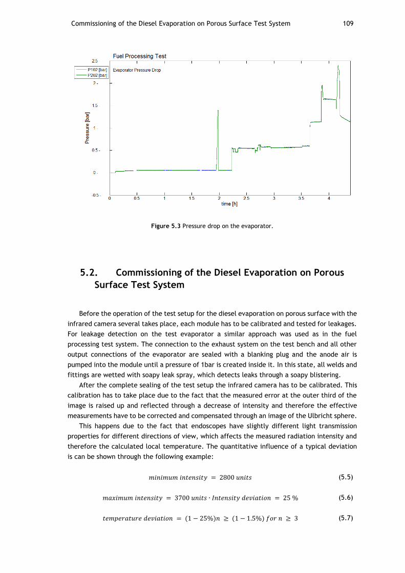
Commissioning of the Diesel Evaporation on Porous Surface Test System 109
Figure 5.3 Pressure drop on the evaporator.
5.2. Commissioning of the Diesel Evaporation on Porous
Surface Test System
Before the operation of the test setup for the diesel evaporation on porous surface with the
infrared camera several takes place, each module has to be calibrated and tested for leakages.
For leakage detection on the test evaporator a similar approach was used as in the fuel
processing test system. The connection to the exhaust system on the test bench and all other
output connections of the evaporator are sealed with a blanking plug and the anode air is
pumped into the module until a pressure of 1bar is created inside it. In this state, all welds and
fittings are wetted with soapy leak spray, which detects leaks through a soapy blistering.
After the complete sealing of the test setup the infrared camera has to be calibrated. This
calibration has to take place due to the fact that the measured error at the outer third of the
image is raised up and reflected through a decrease of intensity and therefore the effective
measurements have to be corrected and compensated through an image of the Ulbricht sphere.
This happens due to the fact that endoscopes have slightly different light transmission
properties for different directions of view, which affects the measured radiation intensity and
therefore the calculated local temperature. The quantitative influence of a typical deviation
is can be shown through the following example:
𝑚𝑖𝑛𝑖𝑚𝑢𝑚 𝑖𝑛𝑡𝑒𝑛𝑠𝑖𝑡𝑦 = 2800 𝑢𝑛𝑖𝑡𝑠 (5.5)
𝑚𝑎𝑥𝑖𝑚𝑢𝑚 𝑖𝑛𝑡𝑒𝑛𝑠𝑖𝑡𝑦 = 3700 𝑢𝑛𝑖𝑡𝑠 ∙ 𝐼𝑛𝑡𝑒𝑛𝑠𝑖𝑡𝑦 𝑑𝑒𝑣𝑖𝑎𝑡𝑖𝑜𝑛 = 25 % (5.6)
𝑡𝑒𝑚𝑝𝑒𝑟𝑎𝑡𝑢𝑟𝑒 𝑑𝑒𝑣𝑖𝑎𝑡𝑖𝑜𝑛 = (1 − 25%)𝑛 ≥ (1 − 1.5%) 𝑓𝑜𝑟 𝑛 ≥ 3 (5.7)
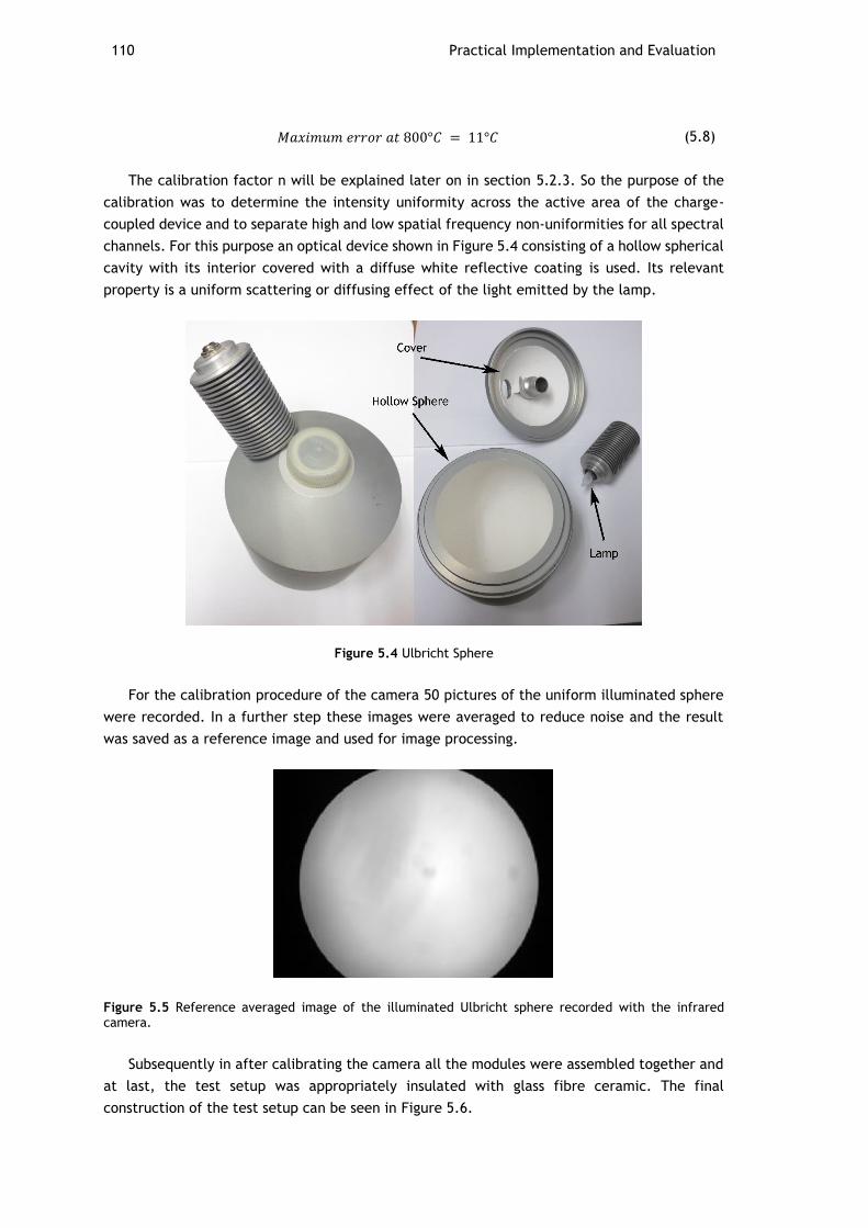
110 Practical Implementation and Evaluation
𝑀𝑎𝑥𝑖𝑚𝑢𝑚 𝑒𝑟𝑟𝑜𝑟 𝑎𝑡 800°𝐶 = 11°𝐶 (5.8)
The calibration factor n will be explained later on in section 5.2.3. So the purpose of the
calibration was to determine the intensity uniformity across the active area of the charge-
coupled device and to separate high and low spatial frequency non-uniformities for all spectral
channels. For this purpose an optical device shown in Figure 5.4 consisting of a hollow spherical
cavity with its interior covered with a diffuse white reflective coating is used. Its relevant
property is a uniform scattering or diffusing effect of the light emitted by the lamp.
Figure 5.4 Ulbricht Sphere
For the calibration procedure of the camera 50 pictures of the uniform illuminated sphere
were recorded. In a further step these images were averaged to reduce noise and the result
was saved as a reference image and used for image processing.
Figure 5.5 Reference averaged image of the illuminated Ulbricht sphere recorded with the infrared camera.
Subsequently in after calibrating the camera all the modules were assembled together and
at last, the test setup was appropriately insulated with glass fibre ceramic. The final
construction of the test setup can be seen in Figure 5.6.
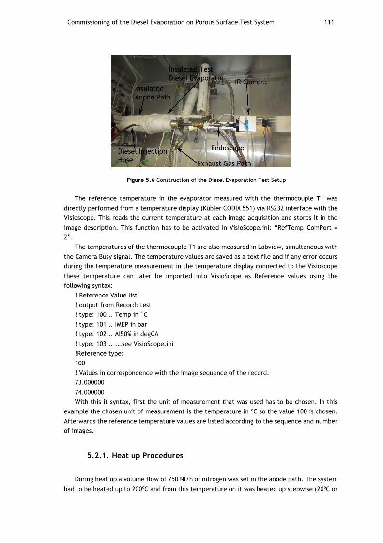
Commissioning of the Diesel Evaporation on Porous Surface Test System 111
Figure 5.6 Construction of the Diesel Evaporation Test Setup
The reference temperature in the evaporator measured with the thermocouple T1 was
directly performed from a temperature display (Kübler CODIX 551) via RS232 interface with the
Visioscope. This reads the current temperature at each image acquisition and stores it in the
image description. This function has to be activated in VisioScope.ini: “RefTemp_ComPort =
2”.
The temperatures of the thermocouple T1 are also measured in Labview, simultaneous with
the Camera Busy signal. The temperature values are saved as a text file and if any error occurs
during the temperature measurement in the temperature display connected to the Visioscope
these temperature can later be imported into VisioScope as Reference values using the
following syntax:
! Reference Value list
! output from Record: test
! type: 100 .. Temp in °C
! type: 101 .. IMEP in bar
! type: 102 .. AI50% in degCA
! type: 103 .. ...see VisioScope.ini
!Reference type:
100
! Values in correspondence with the image sequence of the record:
73.000000
74.000000
With this it syntax, first the unit of measurement that was used has to be chosen. In this
example the chosen unit of measurement is the temperature in ºC so the value 100 is chosen.
Afterwards the reference temperature values are listed according to the sequence and number
of images.
5.2.1. Heat up Procedures
During heat up a volume flow of 750 Nl/h of nitrogen was set in the anode path. The system
had to be heated up to 200ºC and from this temperature on it was heated up stepwise (20ºC or
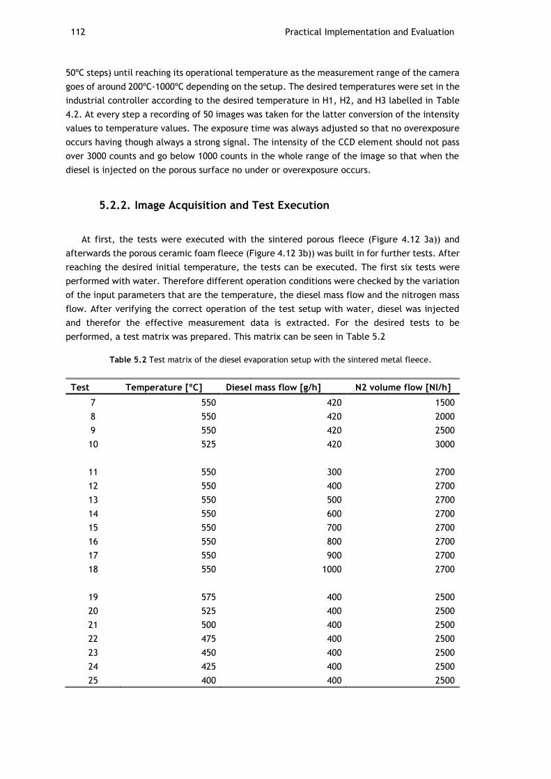
112 Practical Implementation and Evaluation
50ºC steps) until reaching its operational temperature as the measurement range of the camera
goes of around 200ºC-1000ºC depending on the setup. The desired temperatures were set in the
industrial controller according to the desired temperature in H1, H2, and H3 labelled in Table
4.2. At every step a recording of 50 images was taken for the latter conversion of the intensity
values to temperature values. The exposure time was always adjusted so that no overexposure
occurs having though always a strong signal. The intensity of the CCD element should not pass
over 3000 counts and go below 1000 counts in the whole range of the image so that when the
diesel is injected on the porous surface no under or overexposure occurs.
5.2.2. Image Acquisition and Test Execution
At first, the tests were executed with the sintered porous fleece (Figure 4.12 3a)) and
afterwards the porous ceramic foam fleece (Figure 4.12 3b)) was built in for further tests. After
reaching the desired initial temperature, the tests can be executed. The first six tests were
performed with water. Therefore different operation conditions were checked by the variation
of the input parameters that are the temperature, the diesel mass flow and the nitrogen mass
flow. After verifying the correct operation of the test setup with water, diesel was injected
and therefor the effective measurement data is extracted. For the desired tests to be
performed, a test matrix was prepared. This matrix can be seen in Table 5.2
Table 5.2 Test matrix of the diesel evaporation setup with the sintered metal fleece.
Test Temperature [ºC] Diesel mass flow [g/h] N2 volume flow [Nl/h]
7 550 420 1500
8 550 420 2000
9 550 420 2500
10 525 420 3000
11 550 300 2700
12 550 400 2700
13 550 500 2700
14 550 600 2700
15 550 700 2700
16 550 800 2700
17 550 900 2700
18 550 1000 2700
19 575 400 2500
20 525 400 2500
21 500 400 2500
22 475 400 2500
23 450 400 2500
24 425 400 2500
25 400 400 2500
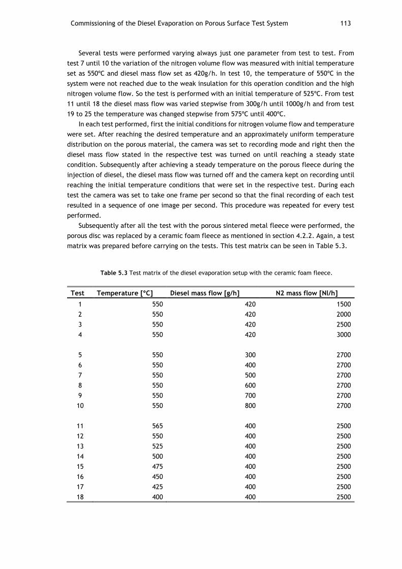
Commissioning of the Diesel Evaporation on Porous Surface Test System 113
Several tests were performed varying always just one parameter from test to test. From
test 7 until 10 the variation of the nitrogen volume flow was measured with initial temperature
set as 550ºC and diesel mass flow set as 420g/h. In test 10, the temperature of 550ºC in the
system were not reached due to the weak insulation for this operation condition and the high
nitrogen volume flow. So the test is performed with an initial temperature of 525ºC. From test
11 until 18 the diesel mass flow was varied stepwise from 300g/h until 1000g/h and from test
19 to 25 the temperature was changed stepwise from 575ºC until 400ºC.
In each test performed, first the initial conditions for nitrogen volume flow and temperature
were set. After reaching the desired temperature and an approximately uniform temperature
distribution on the porous material, the camera was set to recording mode and right then the
diesel mass flow stated in the respective test was turned on until reaching a steady state
condition. Subsequently after achieving a steady temperature on the porous fleece during the
injection of diesel, the diesel mass flow was turned off and the camera kept on recording until
reaching the initial temperature conditions that were set in the respective test. During each
test the camera was set to take one frame per second so that the final recording of each test
resulted in a sequence of one image per second. This procedure was repeated for every test
performed.
Subsequently after all the test with the porous sintered metal fleece were performed, the
porous disc was replaced by a ceramic foam fleece as mentioned in section 4.2.2. Again, a test
matrix was prepared before carrying on the tests. This test matrix can be seen in Table 5.3.
Table 5.3 Test matrix of the diesel evaporation setup with the ceramic foam fleece.
Test Temperature [ºC] Diesel mass flow [g/h] N2 mass flow [Nl/h]
1 550 420 1500
2 550 420 2000
3 550 420 2500
4 550 420 3000
5 550 300 2700
6 550 400 2700
7 550 500 2700
8 550 600 2700
9 550 700 2700
10 550 800 2700
11 565 400 2500
12 550 400 2500
13 525 400 2500
14 500 400 2500
15 475 400 2500
16 450 400 2500
17 425 400 2500
18 400 400 2500
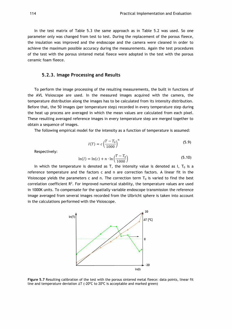
114 Practical Implementation and Evaluation
In the test matrix of Table 5.3 the same approach as in Table 5.2 was used. So one
parameter only was changed from test to test. During the replacement of the porous fleece,
the insulation was improved and the endoscope and the camera were cleaned in order to
achieve the maximum possible accuracy during the measurements. Again the test procedures
of the test with the porous sintered metal fleece were adopted in the test with the porous
ceramic foam fleece.
5.2.3. Image Processing and Results
To perform the image processing of the resulting measurements, the built in functions of
the AVL Visioscope are used. In the measured images acquired with the camera, the
temperature distribution along the images has to be calculated from its intensity distribution.
Before that, the 50 images (per temperature step) recorded in every temperature step during
the heat up process are averaged in which the mean values are calculated from each pixel.
These resulting averaged reference images in every temperature step are merged together to
obtain a sequence of images.
The following empirical model for the intensity as a function of temperature is assumed:
𝐼(𝑇) = 𝑐 (𝑇 − 𝑇0
1000)
𝑛
(5.9)
Respectively:
ln(𝐼) = ln(𝑐) + 𝑛 ∙ ln (𝑇 − 𝑇0
1000) (5.10)
In which the temperature is denoted as T, the intensity value is denoted as I, T0 is a
reference temperature and the factors c and n are correction factors. A linear fit in the
Visioscope yields the parameters c and n. The correction term T0 is varied to find the best
correlation coefficient R2. For improved numerical stability, the temperature values are used
in 1000K units. To compensate for the spatially variable endoscope transmission the reference
image averaged from several images recorded from the Ulbricht sphere is taken into account
in the calculations performed with the Visioscope.
Figure 5.7 Resulting calibration of the test with the porous sintered metal fleece: data points, linear fit line and temperature deviation ΔT (-20ºC to 20ºC is acceptable and marked green)
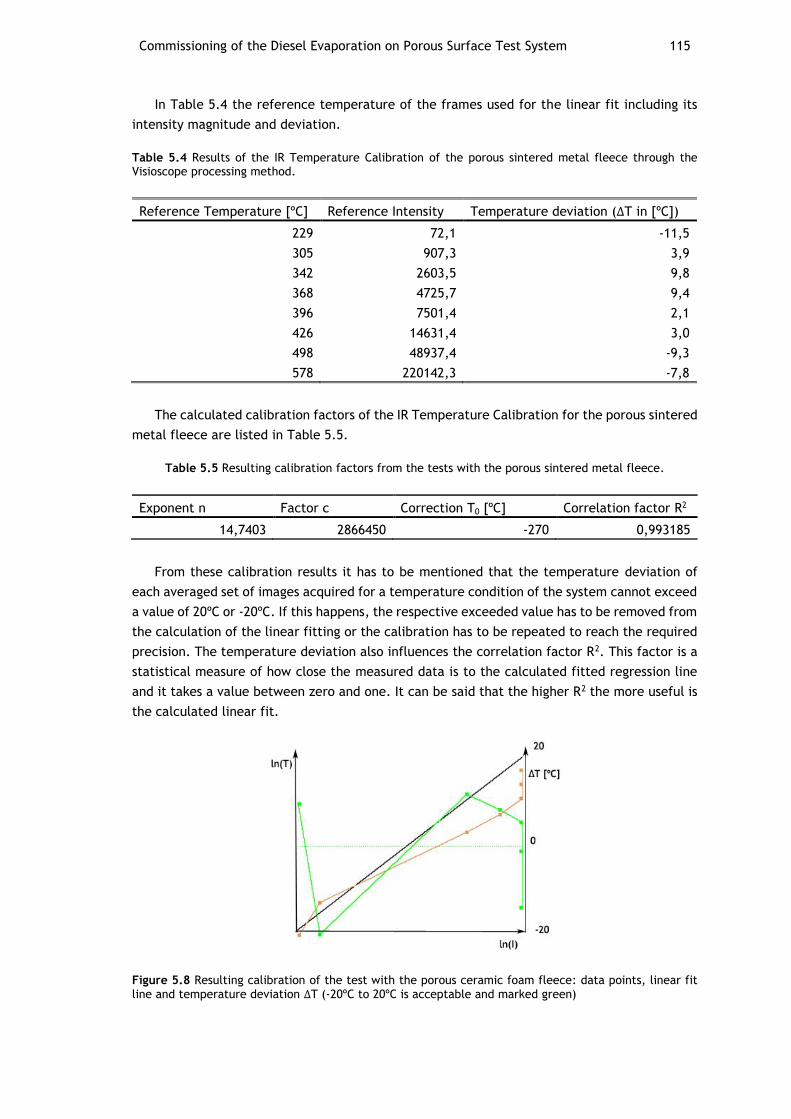
Commissioning of the Diesel Evaporation on Porous Surface Test System 115
In Table 5.4 the reference temperature of the frames used for the linear fit including its
intensity magnitude and deviation.
Table 5.4 Results of the IR Temperature Calibration of the porous sintered metal fleece through the Visioscope processing method.
Reference Temperature [ºC] Reference Intensity Temperature deviation (ΔT in [ºC])
229 72,1 -11,5
305 907,3 3,9
342 2603,5 9,8
368 4725,7 9,4
396 7501,4 2,1
426 14631,4 3,0
498 48937,4 -9,3
578 220142,3 -7,8
The calculated calibration factors of the IR Temperature Calibration for the porous sintered
metal fleece are listed in Table 5.5.
Table 5.5 Resulting calibration factors from the tests with the porous sintered metal fleece.
Exponent n Factor c Correction T0 [ºC] Correlation factor R2
14,7403 2866450 -270 0,993185
From these calibration results it has to be mentioned that the temperature deviation of
each averaged set of images acquired for a temperature condition of the system cannot exceed
a value of 20ºC or -20ºC. If this happens, the respective exceeded value has to be removed from
the calculation of the linear fitting or the calibration has to be repeated to reach the required
precision. The temperature deviation also influences the correlation factor R2. This factor is a
statistical measure of how close the measured data is to the calculated fitted regression line
and it takes a value between zero and one. It can be said that the higher R2 the more useful is
the calculated linear fit.
Figure 5.8 Resulting calibration of the test with the porous ceramic foam fleece: data points, linear fit line and temperature deviation ΔT (-20ºC to 20ºC is acceptable and marked green)
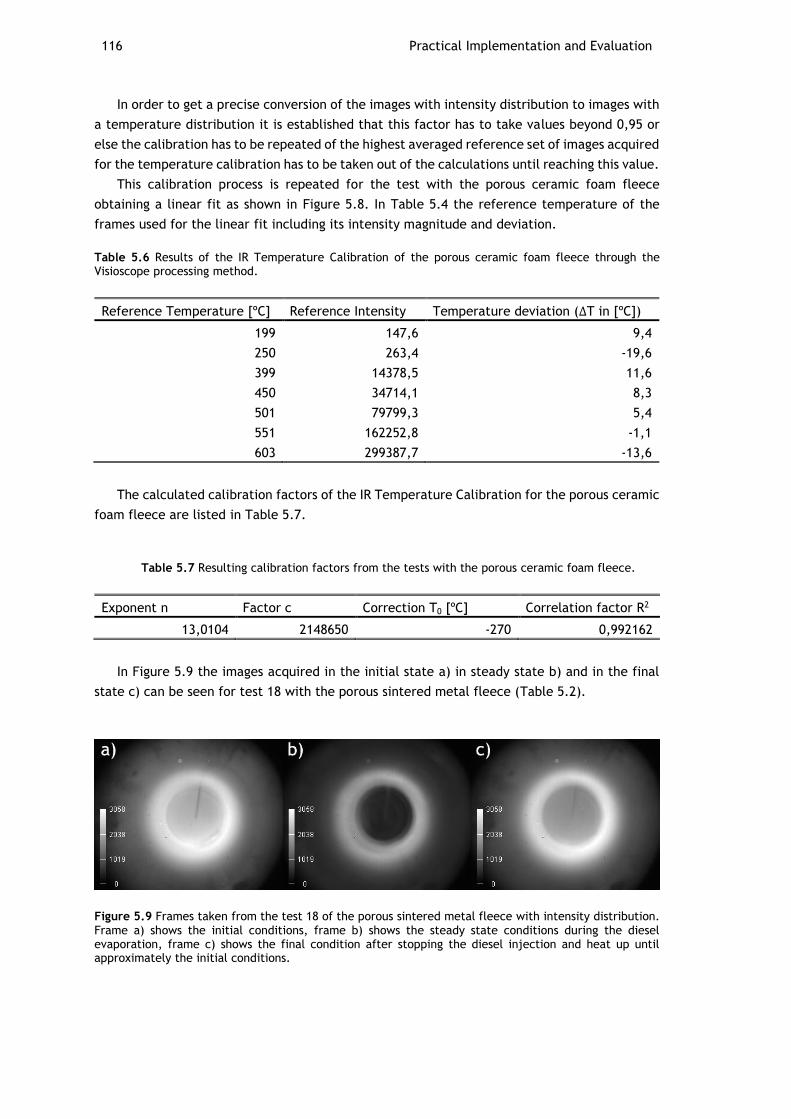
116 Practical Implementation and Evaluation
In order to get a precise conversion of the images with intensity distribution to images with
a temperature distribution it is established that this factor has to take values beyond 0,95 or
else the calibration has to be repeated of the highest averaged reference set of images acquired
for the temperature calibration has to be taken out of the calculations until reaching this value.
This calibration process is repeated for the test with the porous ceramic foam fleece
obtaining a linear fit as shown in Figure 5.8. In Table 5.4 the reference temperature of the
frames used for the linear fit including its intensity magnitude and deviation.
Table 5.6 Results of the IR Temperature Calibration of the porous ceramic foam fleece through the Visioscope processing method.
Reference Temperature [ºC] Reference Intensity Temperature deviation (ΔT in [ºC])
199 147,6 9,4
250 263,4 -19,6
399 14378,5 11,6
450 34714,1 8,3
501 79799,3 5,4
551 162252,8 -1,1
603 299387,7 -13,6
The calculated calibration factors of the IR Temperature Calibration for the porous ceramic
foam fleece are listed in Table 5.7.
Table 5.7 Resulting calibration factors from the tests with the porous ceramic foam fleece.
Exponent n Factor c Correction T0 [ºC] Correlation factor R2
13,0104 2148650 -270 0,992162
In Figure 5.9 the images acquired in the initial state a) in steady state b) and in the final
state c) can be seen for test 18 with the porous sintered metal fleece (Table 5.2).
Figure 5.9 Frames taken from the test 18 of the porous sintered metal fleece with intensity distribution. Frame a) shows the initial conditions, frame b) shows the steady state conditions during the diesel evaporation, frame c) shows the final condition after stopping the diesel injection and heat up until approximately the initial conditions.
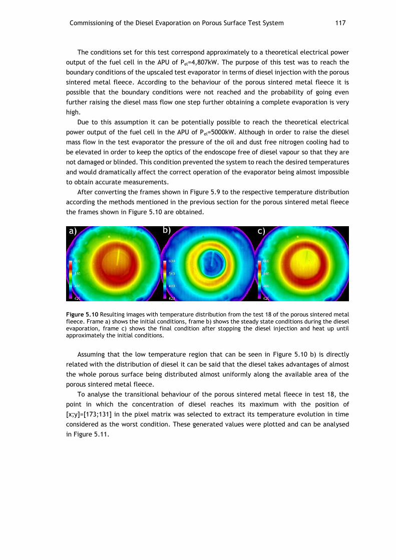
Commissioning of the Diesel Evaporation on Porous Surface Test System 117
The conditions set for this test correspond approximately to a theoretical electrical power
output of the fuel cell in the APU of Pel=4,807kW. The purpose of this test was to reach the
boundary conditions of the upscaled test evaporator in terms of diesel injection with the porous
sintered metal fleece. According to the behaviour of the porous sintered metal fleece it is
possible that the boundary conditions were not reached and the probability of going even
further raising the diesel mass flow one step further obtaining a complete evaporation is very
high.
Due to this assumption it can be potentially possible to reach the theoretical electrical
power output of the fuel cell in the APU of Pel=5000kW. Although in order to raise the diesel
mass flow in the test evaporator the pressure of the oil and dust free nitrogen cooling had to
be elevated in order to keep the optics of the endoscope free of diesel vapour so that they are
not damaged or blinded. This condition prevented the system to reach the desired temperatures
and would dramatically affect the correct operation of the evaporator being almost impossible
to obtain accurate measurements.
After converting the frames shown in Figure 5.9 to the respective temperature distribution
according the methods mentioned in the previous section for the porous sintered metal fleece
the frames shown in Figure 5.10 are obtained.
Figure 5.10 Resulting images with temperature distribution from the test 18 of the porous sintered metal fleece. Frame a) shows the initial conditions, frame b) shows the steady state conditions during the diesel evaporation, frame c) shows the final condition after stopping the diesel injection and heat up until approximately the initial conditions.
Assuming that the low temperature region that can be seen in Figure 5.10 b) is directly
related with the distribution of diesel it can be said that the diesel takes advantages of almost
the whole porous surface being distributed almost uniformly along the available area of the
porous sintered metal fleece.
To analyse the transitional behaviour of the porous sintered metal fleece in test 18, the
point in which the concentration of diesel reaches its maximum with the position of
[x;y]=[173;131] in the pixel matrix was selected to extract its temperature evolution in time
considered as the worst condition. These generated values were plotted and can be analysed
in Figure 5.11.
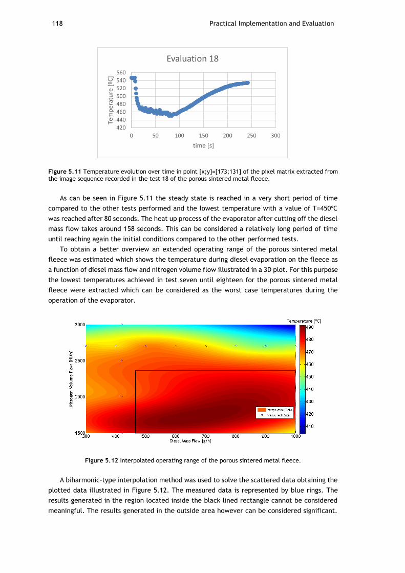
118 Practical Implementation and Evaluation
Figure 5.11 Temperature evolution over time in point [x;y]=[173;131] of the pixel matrix extracted from the image sequence recorded in the test 18 of the porous sintered metal fleece.
As can be seen in Figure 5.11 the steady state is reached in a very short period of time
compared to the other tests performed and the lowest temperature with a value of T=450ºC
was reached after 80 seconds. The heat up process of the evaporator after cutting off the diesel
mass flow takes around 158 seconds. This can be considered a relatively long period of time
until reaching again the initial conditions compared to the other performed tests.
To obtain a better overview an extended operating range of the porous sintered metal
fleece was estimated which shows the temperature during diesel evaporation on the fleece as
a function of diesel mass flow and nitrogen volume flow illustrated in a 3D plot. For this purpose
the lowest temperatures achieved in test seven until eighteen for the porous sintered metal
fleece were extracted which can be considered as the worst case temperatures during the
operation of the evaporator.
Figure 5.12 Interpolated operating range of the porous sintered metal fleece.
A biharmonic-type interpolation method was used to solve the scattered data obtaining the
plotted data illustrated in Figure 5.12. The measured data is represented by blue rings. The
results generated in the region located inside the black lined rectangle cannot be considered
meaningful. The results generated in the outside area however can be considered significant.
420
440
460
480
500
520
540
560
0 50 100 150 200 250 300
Tem
per
atu
re [
ºC]
time [s]
Evaluation 18
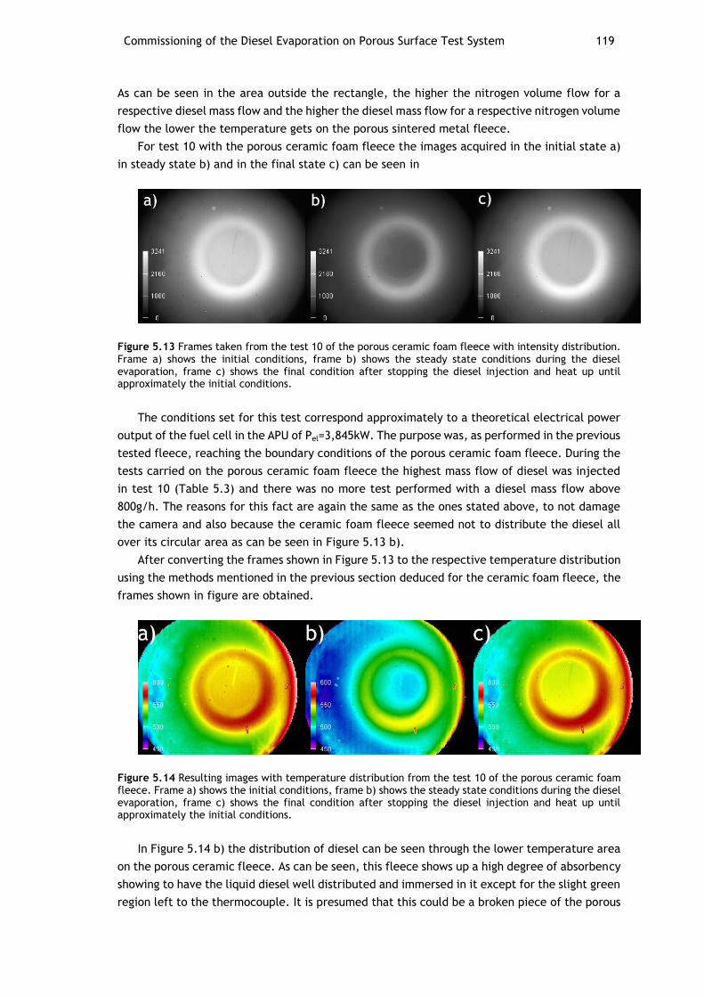
Commissioning of the Diesel Evaporation on Porous Surface Test System 119
As can be seen in the area outside the rectangle, the higher the nitrogen volume flow for a
respective diesel mass flow and the higher the diesel mass flow for a respective nitrogen volume
flow the lower the temperature gets on the porous sintered metal fleece.
For test 10 with the porous ceramic foam fleece the images acquired in the initial state a)
in steady state b) and in the final state c) can be seen in
Figure 5.13 Frames taken from the test 10 of the porous ceramic foam fleece with intensity distribution. Frame a) shows the initial conditions, frame b) shows the steady state conditions during the diesel evaporation, frame c) shows the final condition after stopping the diesel injection and heat up until approximately the initial conditions.
The conditions set for this test correspond approximately to a theoretical electrical power
output of the fuel cell in the APU of Pel=3,845kW. The purpose was, as performed in the previous
tested fleece, reaching the boundary conditions of the porous ceramic foam fleece. During the
tests carried on the porous ceramic foam fleece the highest mass flow of diesel was injected
in test 10 (Table 5.3) and there was no more test performed with a diesel mass flow above
800g/h. The reasons for this fact are again the same as the ones stated above, to not damage
the camera and also because the ceramic foam fleece seemed not to distribute the diesel all
over its circular area as can be seen in Figure 5.13 b).
After converting the frames shown in Figure 5.13 to the respective temperature distribution
using the methods mentioned in the previous section deduced for the ceramic foam fleece, the
frames shown in figure are obtained.
Figure 5.14 Resulting images with temperature distribution from the test 10 of the porous ceramic foam fleece. Frame a) shows the initial conditions, frame b) shows the steady state conditions during the diesel evaporation, frame c) shows the final condition after stopping the diesel injection and heat up until approximately the initial conditions.
In Figure 5.14 b) the distribution of diesel can be seen through the lower temperature area
on the porous ceramic fleece. As can be seen, this fleece shows up a high degree of absorbency
showing to have the liquid diesel well distributed and immersed in it except for the slight green
region left to the thermocouple. It is presumed that this could be a broken piece of the porous
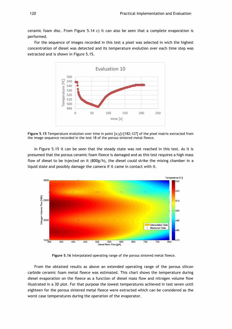
120 Practical Implementation and Evaluation
ceramic foam disc. From Figure 5.14 c) it can also be seen that a complete evaporation is
performed.
For the sequence of images recorded in this test a pixel was selected in wich the highest
concentration of diesel was detected and its temperature evolution over each time step was
extracted and is shown in Figure 5.15.
Figure 5.15 Temperature evolution over time in point [x;y]=[182;127] of the pixel matrix extracted from the image sequence recorded in the test 18 of the porous sintered metal fleece.
In Figure 5.15 it can be seen that the steady state was not reached in this test. As it is
presumed that the porous ceramic foam fleece is damaged and as this test requires a high mass
flow of diesel to be injected on it (800g/h), the diesel could strike the mixing chamber in a
liquid state and possibly damage the camera if it came in contact with it.
Figure 5.16 Interpolated operating range of the porous sintered metal fleece.
From the obtained results as above an extended operating range of the porous silicon
carbide ceramic foam metal fleece was estimated. This chart shows the temperature during
diesel evaporation on the fleece as a function of diesel mass flow and nitrogen volume flow
illustrated in a 3D plot. For that purpose the lowest temperatures achieved in test seven until
eighteen for the porous sintered metal fleece were extracted which can be considered as the
worst case temperatures during the operation of the evaporator.
490
500
510
520
530
540
550
560
0 50 100 150 200 250
Tem
per
atu
re [
ºC]
time [s]
Evaluation 10

Commissioning of the Diesel Evaporation on Porous Surface Test System 121
In order to achieve these results a biharmonic-type interpolation method was used to solve
the scattered data obtaining the plotted data illustrated in Figure 5.16. The measured data is
represented by blue rings. As can be seen the higher the nitrogen volume flow for a respective
diesel mass flow and the higher the diesel mass flow for a respective nitrogen volume flow the
lower the temperature gets on the porous sintered metal fleece.

122 Practical Implementation and Evaluation
123
Chapter 6
Conclusion
In this chapter the achieved goals will be referred. As a complement to the developed work,
suggestions for future tasks that the author recommends to be carried out will be announced.
6.1. Conclusion and Future Work
In the present work, the process of the evaporation through a porous surface and the
mixture formation in a diesel evaporator for the further reaction in an autothermal reformer
for diesel reforming built in a SOFC APU was investigated and optimised. At the starting point
of this work stands the first generation of the diesel evaporator DE-1. As an important resource
for the optimisation of the evaporator computational fluid dynamic modelling (CFD) was used.
The aim of this work was
the development of an optimized evaporator for the operation of an autothermal
diesel reformer with real diesel fuel at the best possible fuel conversion in the long
term.
As intermediate steps the following goals should be achieved:
the optimization of the operating boundary conditions of the evaporator DE-1
the development of a performance-optimized version of the evaporator DE-1,
achieved by structural changes and design modification of the mixing chamber
according to the available space and the possibility of implementation in the APU.
With regard to the objectives the following issues have been worked on:
homogeneous mixture of the anode gas and fuel in the gas phase,
injection, distribution and atomization of the fuel droplets on a porous surface,
complete vaporization of the fuel, and
suppression and prevention of possible soot formation and establishment of
carbonaceous deposits.
These issues are strongly related to each other. Through a Matlab Simulink simulation
several parameters for the operation of the evaporator inside the APU were extracted. Based
on a modelled CFD-simulation of the DE-1 the weak points of its construction were identified.
The mixing chamber of the DE-1 was modified to compensate its negative effects and prepared
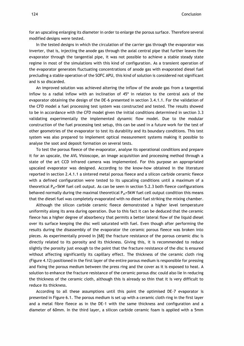
124 Conclusion
for an upscaling enlarging its diameter in order to enlarge the porous surface. Therefore several
modified designs were tested.
In the tested designs in which the circulation of the carrier gas through the evaporator was
inverter, that is, injecting the anode gas through the axial central pipe that further leaves the
evaporator through the tangential pipe, it was not possible to achieve a stable steady state
regime in most of the simulations with this kind of configuration. As a transient operation of
the evaporator generates fluctuating concentrations of anode gas with evaporated diesel fuel
precluding a stable operation of the SOFC APU, this kind of solution is considered not significant
and is so discarded.
An improved solution was achieved altering the inflow of the anode gas from a tangential
inflow to a radial inflow with an inclination of 45º in relation to the central axis of the
evaporator obtaining the design of the DE-6 presented in section 3.4.1.1. For the validation of
the CFD model a fuel processing test system was constructed and tested. The results showed
to be in accordance with the CFD model given the initial conditions determined in section 3.3
validating experimentally the implemented dynamic flow model. Due to the modular
construction of the fuel processing test setup, this can be used in a future work for the test of
other geometries of the evaporator to test its durability and its boundary conditions. This test
system was also prepared to implement optical measurement systems making it possible to
analyse the soot and deposit formation on several tests.
To test the porous fleece of the evaporator, analyse its operational conditions and prepare
it for an upscale, the AVL Visioscope, an image acquisition and processing method through a
state of the art CCD infrared camera was implemented. For this purpose an appropriated
upscaled evaporator was designed. According to the know-how obtained in the literature
reported in section 2.4.1.1 a sintered metal porous fleece and a silicon carbide ceramic fleece
with a defined configuration were tested to its upscaling conditions until a maximum of a
theoretical Pel=5kW fuel cell output. As can be seen in section 5.2.3 both fleece configurations
behaved normally during the maximal theoretical Pel=5kW fuel cell output condition this means
that the diesel fuel was completely evaporated with no diesel fuel striking the mixing chamber.
Although the silicon carbide ceramic fleece demonstrated a higher level temperature
uniformity along its area during operation. Due to this fact it can be deduced that the ceramic
fleece has a higher degree of absorbency that permits a better lateral flow of the liquid diesel
over its surface keeping the disc well saturated with fuel. Even though after performing the
results during the disassembly of the evaporator the ceramic porous fleece was broken into
pieces. As experimentally proved in [68] the fracture resistance of the porous ceramic disc is
directly related to its porosity and its thickness. Giving this, it is recommended to reduce
slightly the porosity just enough to the point that the fracture resistance of the disc is ensured
without affecting significantly its capillary effect. The thickness of the ceramic cloth ring
(Figure 4.12) positioned in the first layer of the entire porous medium is responsible for pressing
and fixing the porous medium between the press ring and the cover as it is exposed to heat. A
solution to enhance the fracture resistance of the ceramic porous disc could also lie in reducing
the thickness of the ceramic cloth, although this is already so thin that it is very difficult to
reduce its thickness.
According to all these assumptions until this point the optimised DE-7 evaporator is
presented in Figure 6.1. The porous medium is set up with a ceramic cloth ring in the first layer
and a metal fibre fleece as in the DE-1 with the same thickness and configuration and a
diameter of 60mm. In the third layer, a silicon carbide ceramic foam is applied with a 5mm
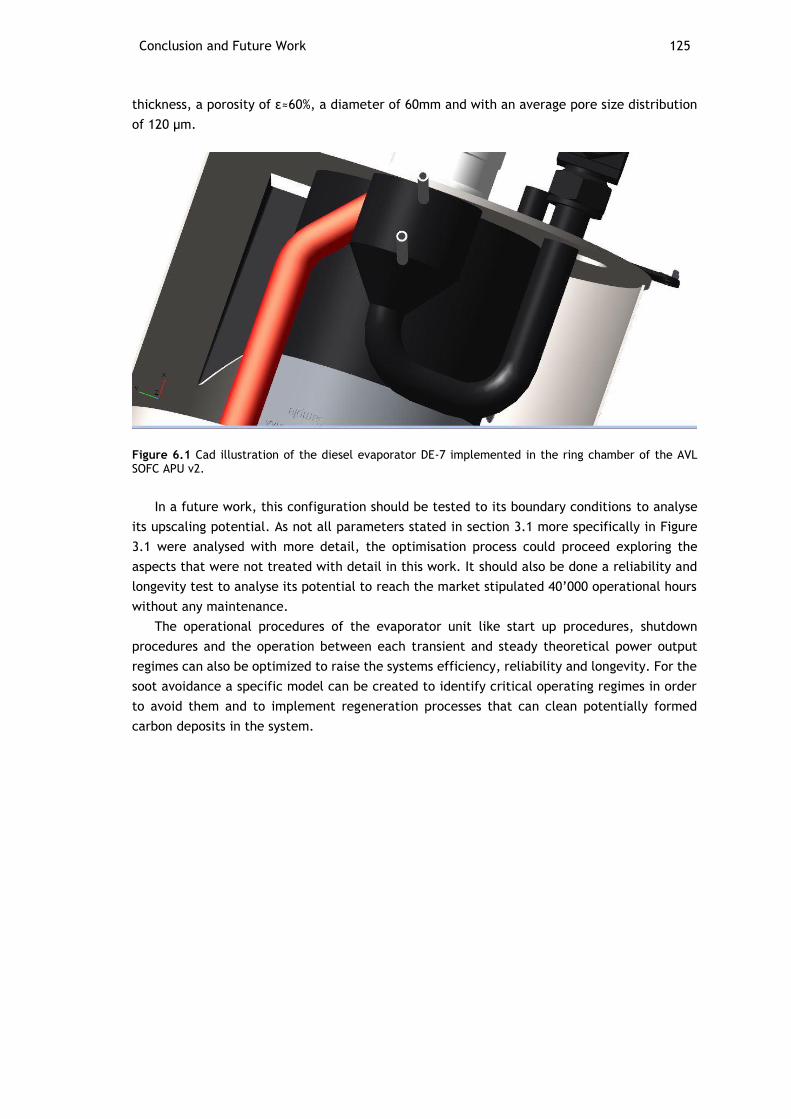
Conclusion and Future Work 125
thickness, a porosity of ε≈60%, a diameter of 60mm and with an average pore size distribution
of 120 µm.
Figure 6.1 Cad illustration of the diesel evaporator DE-7 implemented in the ring chamber of the AVL SOFC APU v2.
In a future work, this configuration should be tested to its boundary conditions to analyse
its upscaling potential. As not all parameters stated in section 3.1 more specifically in Figure
3.1 were analysed with more detail, the optimisation process could proceed exploring the
aspects that were not treated with detail in this work. It should also be done a reliability and
longevity test to analyse its potential to reach the market stipulated 40’000 operational hours
without any maintenance.
The operational procedures of the evaporator unit like start up procedures, shutdown
procedures and the operation between each transient and steady theoretical power output
regimes can also be optimized to raise the systems efficiency, reliability and longevity. For the
soot avoidance a specific model can be created to identify critical operating regimes in order
to avoid them and to implement regeneration processes that can clean potentially formed
carbon deposits in the system.

126 Conclusion
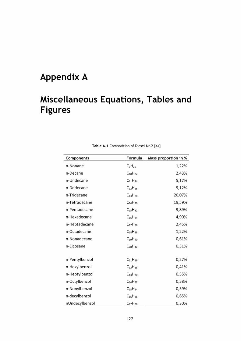
127
Appendix A
Miscellaneous Equations, Tables and Figures
Table A.1 Composition of Diesel Nr.2 [44]
Components Formula Mass proportion in %
n-Nonane C9H20 1,22%
n-Decane C10H22 2,43%
n-Undecane C11H24 5,17%
n-Dodecane C12H26 9,12%
n-Tridecane C13H28 20,07%
n-Tetradecane C14H30 19,59%
n-Pentadecane C15H32 9,89%
n-Hexadecane C16H34 4,90%
n-Heptadecane C17H36 2,45%
n-Octadecane C18H38 1,22%
n-Nonadecane C19H40 0,61%
n-Eicosane C20H42 0,31%
n-Pentylbenzol C11H16 0,27%
n-Hexylbenzol C12H18 0,41%
n-Heptylbenzol C13H20 0,55%
n-Octylbenzol C14H22 0,58%
n-Nonylbenzol C15H24 0,59%
n-decylbenzol C16H26 0,65%
nUndecylbenzol C17H28 0,30%
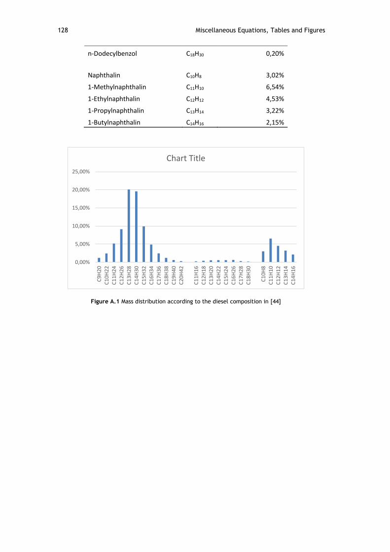
128 Miscellaneous Equations, Tables and Figures
n-Dodecylbenzol C18H30 0,20%
Naphthalin C10H8 3,02%
1-Methylnaphthalin C11H10 6,54%
1-Ethylnaphthalin C12H12 4,53%
1-Propylnaphthalin C13H14 3,22%
1-Butylnaphthalin C14H16 2,15%
Figure A.1 Mass distribution according to the diesel composition in [44]
0,00%
5,00%
10,00%
15,00%
20,00%
25,00%
C9
H2
0
C1
0H
22
C1
1H
24
C1
2H
26
C1
3H
28
C1
4H
30
C1
5H
32
C1
6H
34
C1
7H
36
C1
8H
38
C1
9H
40
C2
0H
42
C1
1H
16
C1
2H
18
C1
3H
20
C1
4H
22
C1
5H
24
C1
6H
26
C1
7H
28
C1
8H
30
C1
0H
8
C1
1H
10
C1
2H
12
C1
3H
14
C1
4H
16
Chart Title
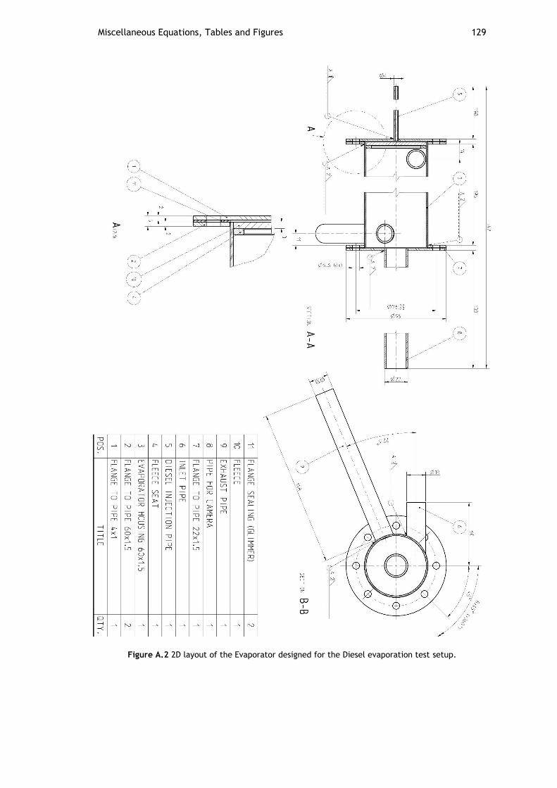
Miscellaneous Equations, Tables and Figures 129
Figure A.2 2D layout of the Evaporator designed for the Diesel evaporation test setup.
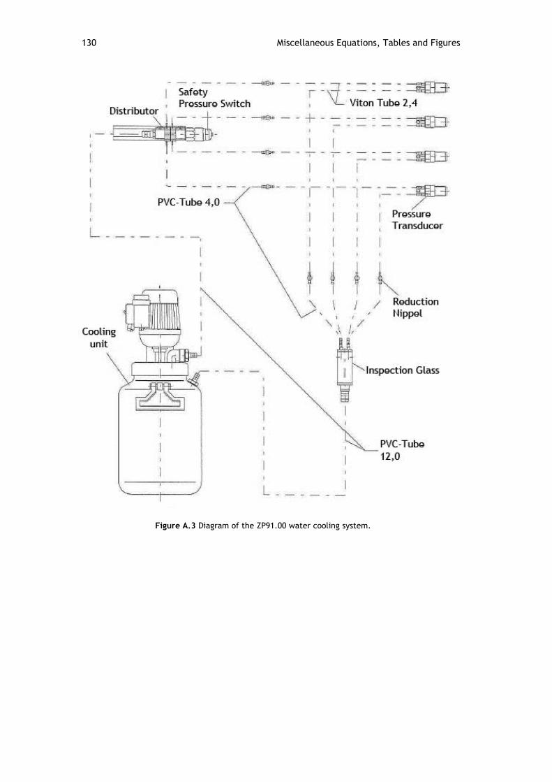
130 Miscellaneous Equations, Tables and Figures
Figure A.3 Diagram of the ZP91.00 water cooling system.
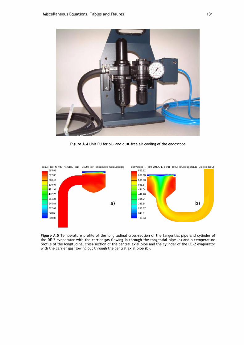
Miscellaneous Equations, Tables and Figures 131
Figure A.4 Unit FU for oil- and dust-free air cooling of the endoscope
Figure A.5 Temperature profile of the longitudinal cross-section of the tangential pipe and cylinder of the DE-2 evaporator with the carrier gas flowing in through the tangential pipe (a) and a temperature profile of the longitudinal cross-section of the central axial pipe and the cylinder of the DE-2 evaporator with the carrier gas flowing out through the central axial pipe (b).
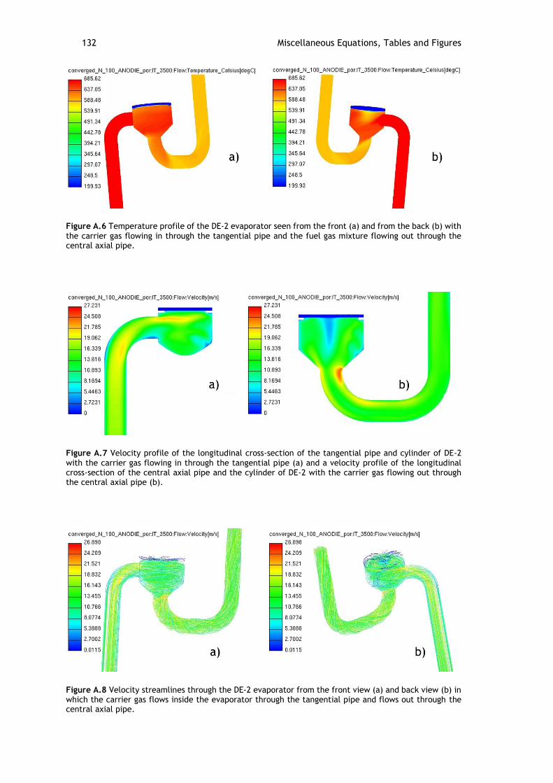
132 Miscellaneous Equations, Tables and Figures
Figure A.6 Temperature profile of the DE-2 evaporator seen from the front (a) and from the back (b) with the carrier gas flowing in through the tangential pipe and the fuel gas mixture flowing out through the central axial pipe.
Figure A.7 Velocity profile of the longitudinal cross-section of the tangential pipe and cylinder of DE-2 with the carrier gas flowing in through the tangential pipe (a) and a velocity profile of the longitudinal cross-section of the central axial pipe and the cylinder of DE-2 with the carrier gas flowing out through the central axial pipe (b).
Figure A.8 Velocity streamlines through the DE-2 evaporator from the front view (a) and back view (b) in which the carrier gas flows inside the evaporator through the tangential pipe and flows out through the central axial pipe.
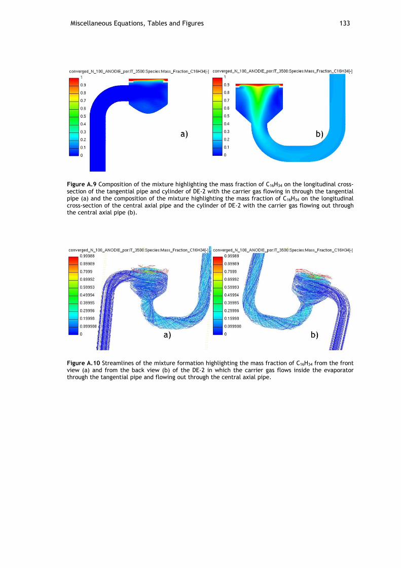
Miscellaneous Equations, Tables and Figures 133
Figure A.9 Composition of the mixture highlighting the mass fraction of C16H34 on the longitudinal cross-section of the tangential pipe and cylinder of DE-2 with the carrier gas flowing in through the tangential pipe (a) and the composition of the mixture highlighting the mass fraction of C16H34 on the longitudinal cross-section of the central axial pipe and the cylinder of DE-2 with the carrier gas flowing out through the central axial pipe (b).
Figure A.10 Streamlines of the mixture formation highlighting the mass fraction of C16H34 from the front view (a) and from the back view (b) of the DE-2 in which the carrier gas flows inside the evaporator through the tangential pipe and flowing out through the central axial pipe.
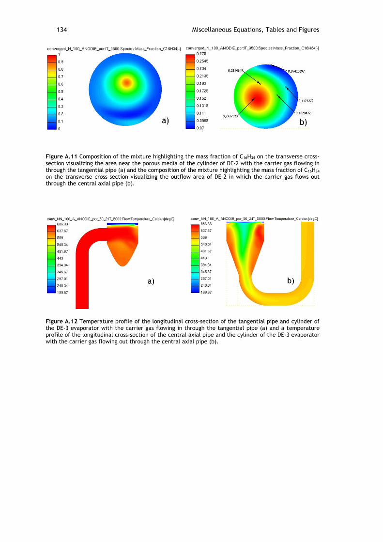
134 Miscellaneous Equations, Tables and Figures
Figure A.11 Composition of the mixture highlighting the mass fraction of C16H34 on the transverse cross-section visualizing the area near the porous media of the cylinder of DE-2 with the carrier gas flowing in through the tangential pipe (a) and the composition of the mixture highlighting the mass fraction of C16H34 on the transverse cross-section visualizing the outflow area of DE-2 in which the carrier gas flows out through the central axial pipe (b).
Figure A.12 Temperature profile of the longitudinal cross-section of the tangential pipe and cylinder of the DE-3 evaporator with the carrier gas flowing in through the tangential pipe (a) and a temperature profile of the longitudinal cross-section of the central axial pipe and the cylinder of the DE-3 evaporator with the carrier gas flowing out through the central axial pipe (b).
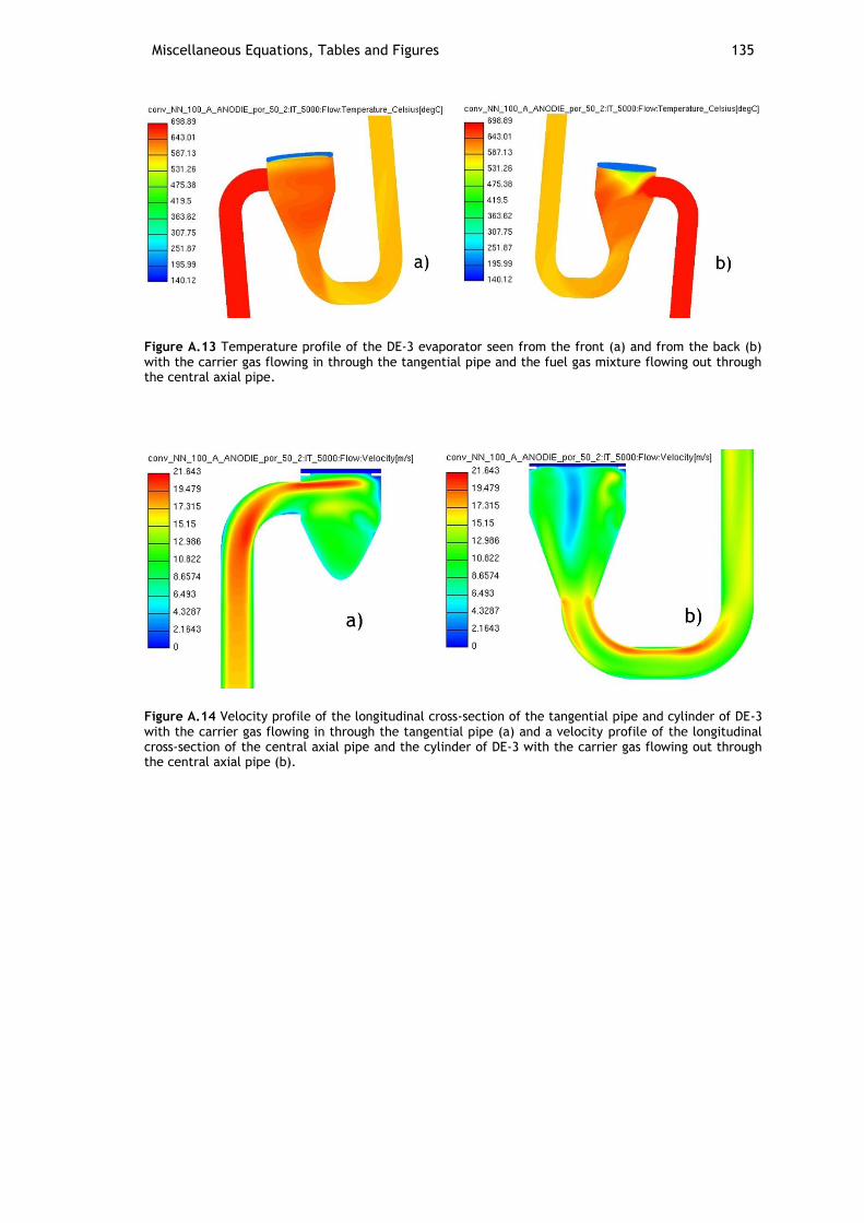
Miscellaneous Equations, Tables and Figures 135
Figure A.13 Temperature profile of the DE-3 evaporator seen from the front (a) and from the back (b) with the carrier gas flowing in through the tangential pipe and the fuel gas mixture flowing out through the central axial pipe.
Figure A.14 Velocity profile of the longitudinal cross-section of the tangential pipe and cylinder of DE-3 with the carrier gas flowing in through the tangential pipe (a) and a velocity profile of the longitudinal cross-section of the central axial pipe and the cylinder of DE-3 with the carrier gas flowing out through the central axial pipe (b).
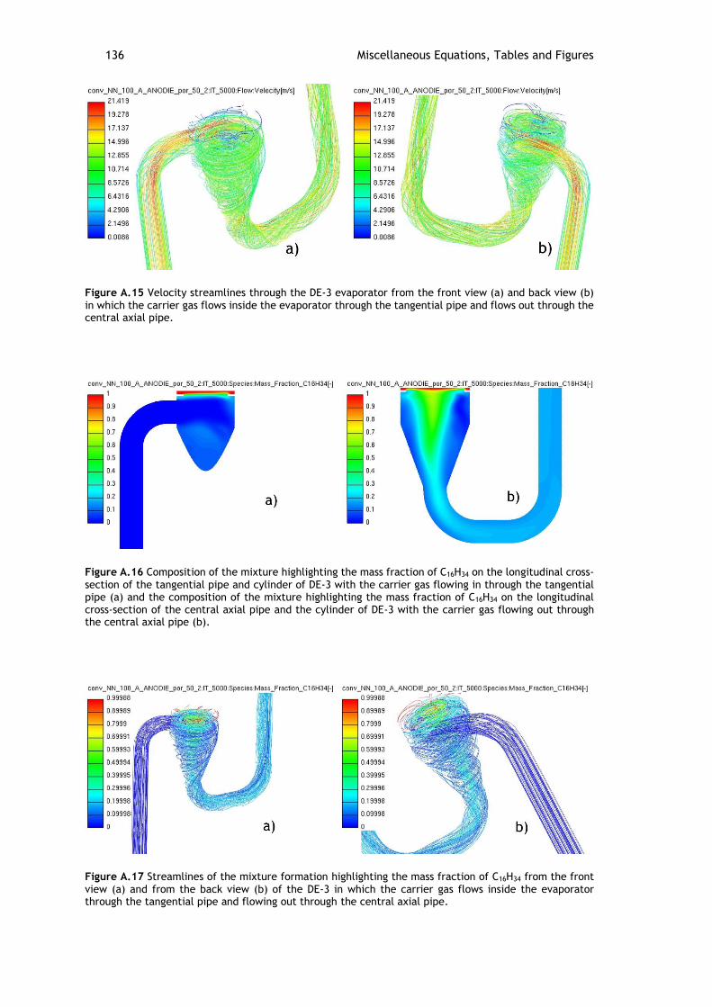
136 Miscellaneous Equations, Tables and Figures
Figure A.15 Velocity streamlines through the DE-3 evaporator from the front view (a) and back view (b) in which the carrier gas flows inside the evaporator through the tangential pipe and flows out through the central axial pipe.
Figure A.16 Composition of the mixture highlighting the mass fraction of C16H34 on the longitudinal cross-section of the tangential pipe and cylinder of DE-3 with the carrier gas flowing in through the tangential pipe (a) and the composition of the mixture highlighting the mass fraction of C16H34 on the longitudinal cross-section of the central axial pipe and the cylinder of DE-3 with the carrier gas flowing out through the central axial pipe (b).
Figure A.17 Streamlines of the mixture formation highlighting the mass fraction of C16H34 from the front view (a) and from the back view (b) of the DE-3 in which the carrier gas flows inside the evaporator through the tangential pipe and flowing out through the central axial pipe.
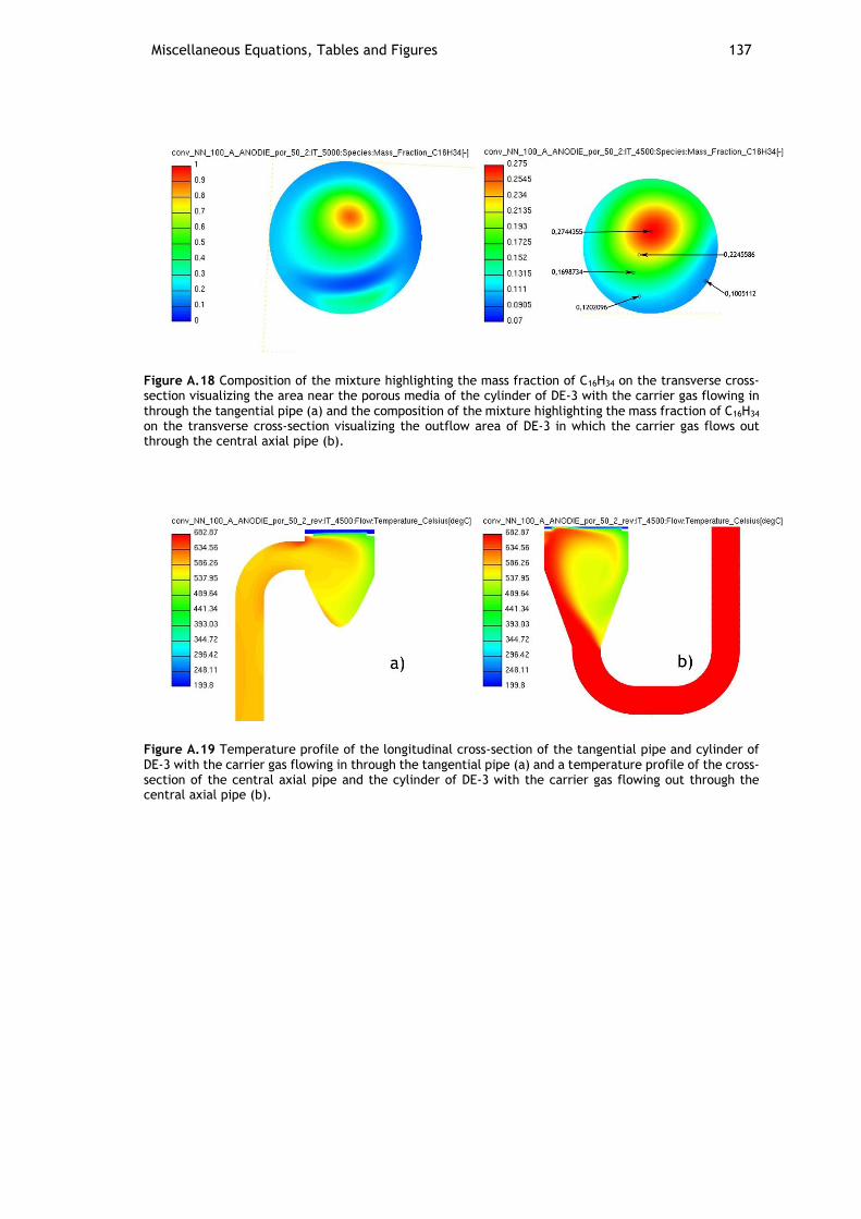
Miscellaneous Equations, Tables and Figures 137
Figure A.18 Composition of the mixture highlighting the mass fraction of C16H34 on the transverse cross-section visualizing the area near the porous media of the cylinder of DE-3 with the carrier gas flowing in through the tangential pipe (a) and the composition of the mixture highlighting the mass fraction of C16H34 on the transverse cross-section visualizing the outflow area of DE-3 in which the carrier gas flows out through the central axial pipe (b).
Figure A.19 Temperature profile of the longitudinal cross-section of the tangential pipe and cylinder of DE-3 with the carrier gas flowing in through the tangential pipe (a) and a temperature profile of the cross-section of the central axial pipe and the cylinder of DE-3 with the carrier gas flowing out through the central axial pipe (b).
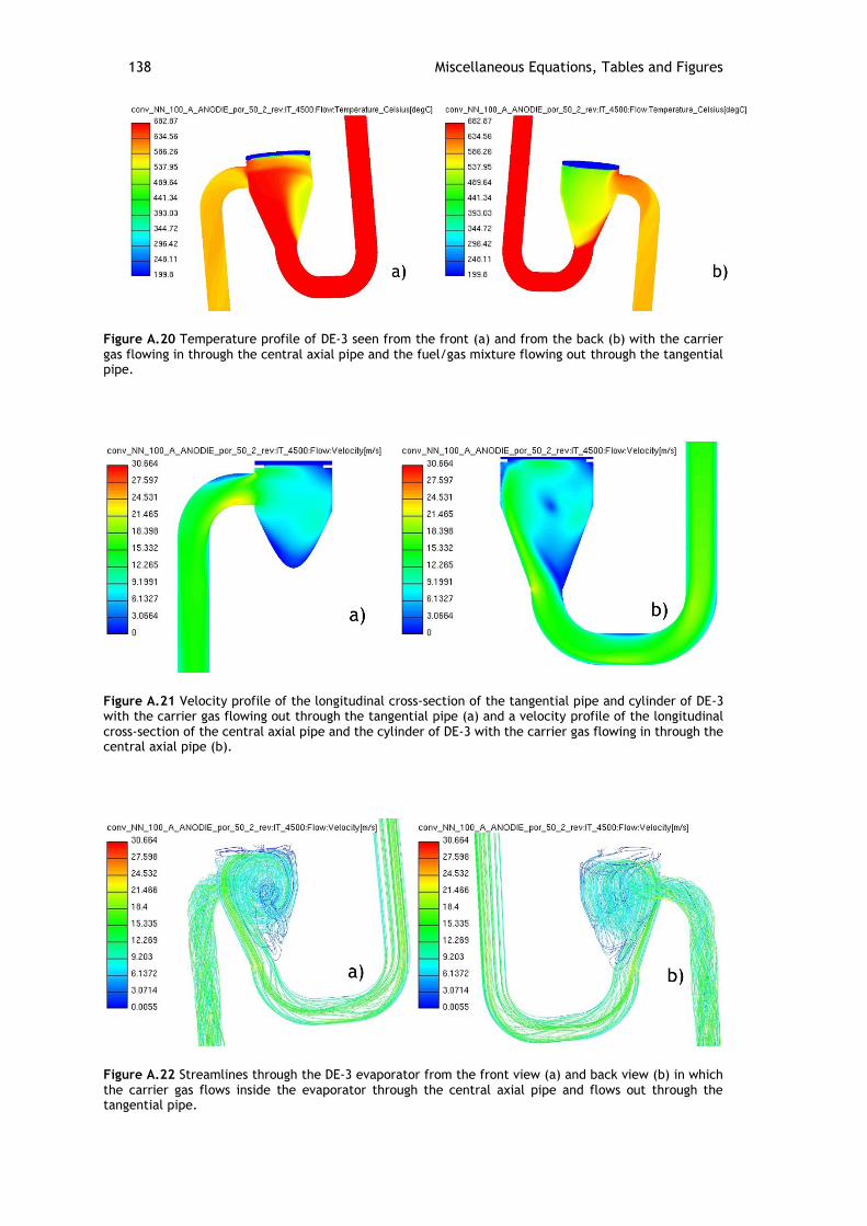
138 Miscellaneous Equations, Tables and Figures
Figure A.20 Temperature profile of DE-3 seen from the front (a) and from the back (b) with the carrier gas flowing in through the central axial pipe and the fuel/gas mixture flowing out through the tangential pipe.
Figure A.21 Velocity profile of the longitudinal cross-section of the tangential pipe and cylinder of DE-3 with the carrier gas flowing out through the tangential pipe (a) and a velocity profile of the longitudinal cross-section of the central axial pipe and the cylinder of DE-3 with the carrier gas flowing in through the central axial pipe (b).
Figure A.22 Streamlines through the DE-3 evaporator from the front view (a) and back view (b) in which the carrier gas flows inside the evaporator through the central axial pipe and flows out through the tangential pipe.
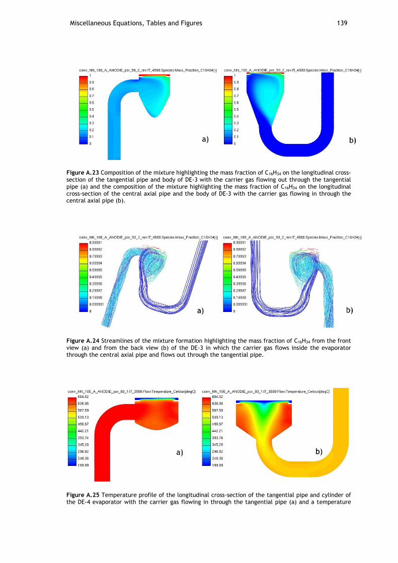
Miscellaneous Equations, Tables and Figures 139
Figure A.23 Composition of the mixture highlighting the mass fraction of C16H34 on the longitudinal cross-section of the tangential pipe and body of DE-3 with the carrier gas flowing out through the tangential pipe (a) and the composition of the mixture highlighting the mass fraction of C16H34 on the longitudinal cross-section of the central axial pipe and the body of DE-3 with the carrier gas flowing in through the central axial pipe (b).
Figure A.24 Streamlines of the mixture formation highlighting the mass fraction of C16H34 from the front view (a) and from the back view (b) of the DE-3 in which the carrier gas flows inside the evaporator through the central axial pipe and flows out through the tangential pipe.
Figure A.25 Temperature profile of the longitudinal cross-section of the tangential pipe and cylinder of the DE-4 evaporator with the carrier gas flowing in through the tangential pipe (a) and a temperature
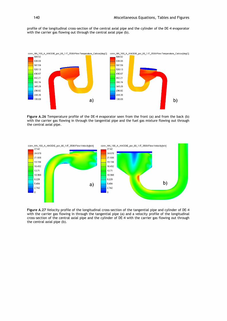
140 Miscellaneous Equations, Tables and Figures
profile of the longitudinal cross-section of the central axial pipe and the cylinder of the DE-4 evaporator with the carrier gas flowing out through the central axial pipe (b).
Figure A.26 Temperature profile of the DE-4 evaporator seen from the front (a) and from the back (b) with the carrier gas flowing in through the tangential pipe and the fuel gas mixture flowing out through the central axial pipe.
Figure A.27 Velocity profile of the longitudinal cross-section of the tangential pipe and cylinder of DE-4 with the carrier gas flowing in through the tangential pipe (a) and a velocity profile of the longitudinal cross-section of the central axial pipe and the cylinder of DE-4 with the carrier gas flowing out through the central axial pipe (b).
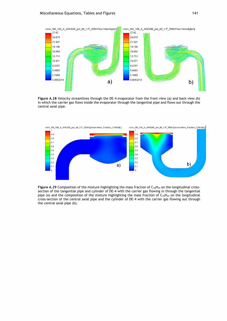
Miscellaneous Equations, Tables and Figures 141
Figure A.28 Velocity streamlines through the DE-4 evaporator from the front view (a) and back view (b) in which the carrier gas flows inside the evaporator through the tangential pipe and flows out through the central axial pipe.
Figure A.29 Composition of the mixture highlighting the mass fraction of C16H34 on the longitudinal cross-section of the tangential pipe and cylinder of DE-4 with the carrier gas flowing in through the tangential pipe (a) and the composition of the mixture highlighting the mass fraction of C16H34 on the longitudinal cross-section of the central axial pipe and the cylinder of DE-4 with the carrier gas flowing out through the central axial pipe (b).
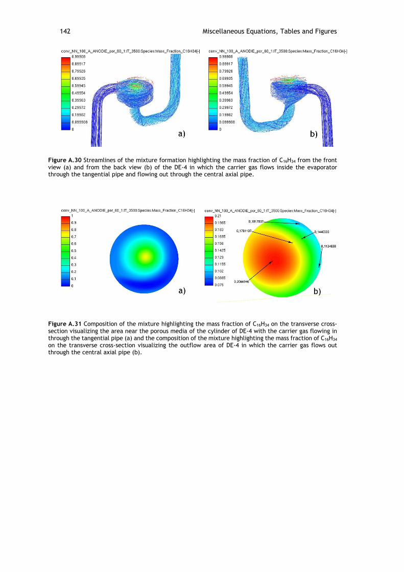
142 Miscellaneous Equations, Tables and Figures
Figure A.30 Streamlines of the mixture formation highlighting the mass fraction of C16H34 from the front view (a) and from the back view (b) of the DE-4 in which the carrier gas flows inside the evaporator through the tangential pipe and flowing out through the central axial pipe.
Figure A.31 Composition of the mixture highlighting the mass fraction of C16H34 on the transverse cross-section visualizing the area near the porous media of the cylinder of DE-4 with the carrier gas flowing in through the tangential pipe (a) and the composition of the mixture highlighting the mass fraction of C16H34 on the transverse cross-section visualizing the outflow area of DE-4 in which the carrier gas flows out through the central axial pipe (b).
143
Bibliography
[1] A. M. Heinzel, J.; Dokupil, M.; Roes, J, "Problemstellung, Chancen und Risiken von
Brennstoffzellen APU's," Ostbayerisches Technologie-Transfer-Institut 2003.
[2] J. T. P. Lamp, O. Finkenwirth, S. Mukerjee, S. Shaffer, "Development of an Auxiliary
Power Unit with Solid Oxide Fuel Cells for Automotive Applications," Fuel Cells vol. 3,
2003.
[3] R. H. Perry and D. W. Green, Perry's Chemical Engineers' Handbook, Eighth Edition:
McGraw-Hill, 2008.
[4] T. K. Mandal and D. H. Gregory, "Hydrogen: a future energy vector for sustainable
development," Proceedings of the Institution of Mechanical Engineers Part C: Journal
of Mechanical Engineering Science, vol. 224, pp. 539-558, 2010.
[5] S. S. J. Zizelman, and S. Mukerjee, "Solid oxide fuel cell auxiliary power unit -- a
development update," Society of Automotive Engineers, 2002.
[6] A. L. S. Kah, "Fuel Processor for catalytic partial oxidation and combustion of
hydrocarbons," Fuel Cells Science and Technology, 2004.
[7] J. Lawrence and M. Boltze, "Auxiliary power unit based on a solid oxide fuel cell and
fuelled with diesel," Journal of Power Sources, vol. 154, pp. 479-488, 3/21/ 2006.
[8] L. L. Zoran Filipi, Anna Stefanopoulou, Jay Pukrushpan, Burit Kittirungsi and Huei Peng,
"Fuel Cell APU for Silent Watch and Mild Electrification of a Medium Tactical Truck,"
Automotive Research Center University of Michigan, 2004.
[9] T. Grube, R. Menzer, and R. Peters, "Pkw-Bordstromversorgung mit Brennstoffzellen-
APU - Eine Bewertung mit Blick auf den Wirkungsgrad," Brennstoff, Wärme, Kraft
(BWK), vol. 58, 2006.
[10] M. Reißig, "Entwicklung einer Kombinierten Diesel Reformer-Brennereinheit für eine
SOFC APU " 2010.
[11] W. R. Grove, "Journal fo science," Philosofical Magazine, vol. 14, pp. 126-131, 1839.
[12] L. M. a. C. Langer, "Proceedings of the Royal Society of London," vol. 46, pp. 296-304,
1889.
[13] W. Ostwald, "Zeitschrift für Elektrotechnik und Elektrochemie," vol. 1, pp. 122-125,
1894.
[14] H. P. Emil Baur, "Über Brennstoff-Ketten mit Festleitern," Zeitschrift für Elektrochemie
und angewandte physikalische Chemie, vol. 43, pp. 727–732, 1937.
[15] O. Davtyan, "Acad. Sci. USSR," Sci. Technol., pp. 107-114, 1946.
[16] N. Q. Minh, "Ceramic Fuel Cells," Journal of the American Ceramic Society, vol. 76, pp.
563–588, 1993.
[17] I. EG&G Technical Services, "Fuel Cell Handbook (Seventh Edition)," U.S. Department
of Energy, 2004.
[18] F. M. K. Ledjeff-Hey, J. Roes, "Brennstoffzellen: Entwicklung, Technologie," Müller-
Verlag, 2001.
[19] J. L. A. Dicks, "Fuel Cell Systems Explained," Wiley, 2003.
[20] M. Dokiya, "SOFC system and technology," Solid State Ionics, vol. 152–153, pp. 383–392,
2002.
[21] W. K. J.-F. Hake, K. Kugeler, W. Pfaffenberg, H.-J. Wagner, "Vorlesungsmanuskripte
zum 4. Ferienkurs im Forschungszentrum Jülich," p. 256, 1998.
[22] N. Q. Minh and T. Takahashi, Science and Technology of Ceramic Fuel Cells: Elsevier
Science, 1995.
[23] F. E. v. Brennstoffzellen and O. Technologie-Transfer-Institut, Einsatz von
Brennstoffzellen: sechstes Fachforum, 04./05. Oktober 1999, Leipzig: Ostbayerisches
Technologie Transfer Institut, OTTI, 1999.
[24] B. C. Gates, J. R. Katzer, and G. C. A. Schuit, Chemistry of catalytic processes:
McGraw-Hill, 1979.
[25] Y. Jamal and M. L. Wyszynski, "On-board generation of hydrogen-rich gaseous fuels—a
review," International Journal of Hydrogen Energy, vol. 19, pp. 557-572, 7// 1994.
144 Bibliography
[26] R. P. J. Pasel, T. Alcher, "Wasserstofferzeugung aus Dieselkraftstoffen," FVS Themen,
2004.
[27] D. V. Edlund, "Versatile, low-cost and compact fuel processor for low-temperature fuel
cells," Fuel Cells Bulletin Band 2, vol. Heft 14 pp. 8-11, 1999.
[28] M. H. Hrsg.: Baerns, H.; Renken, A., "Chemische Reaktionstechnik (Lehrbuch der
Technischen Chemie Band 1)," Georg Thieme Verlag Stuttgart, vol. 2. Auflage, 1992.
[29] C. Schlitzberger, "Solid Oxide Fuel Cell (SOFC)-Systeme mit integrierter Reformierung
bzw. Vergasung von Kohlenwasserstoffen," 2012.
[30] A. F. Ghenciu, "Review of fuel processing catalysts for hydrogen production in PEM fuel
cell systems," Current Opinion in Solid State and Materials Science vol. 6, pp. 389-399,
2002.
[31] T. R. K. M. Krumpelt∗, J.D. Carter, J.P. Kopasz, S. Ahmed, "Fuel processing for fuel cell
systems in transportation and portable power applications," Catalysis Today, 2002.
[32] N. Iwasa, W. Nomura, T. Mayanagi, S.-i. Fujita, M. Arai, and N. Takezawa, "Hydrogen
Production by Steam Reforming of Methanol," JOURNAL OF CHEMICAL ENGINEERING OF
JAPAN, vol. 37, pp. 286-293, 2004.
[33] S. Wieland, Baumann, F., and Starz, K., "New Powerful Catalysts for Autothermal
Reforming of Hydrocarbons and Water-Gas Shift Reaction for On-board Hydrogen
Generation in Automotive PEMFC Applications," SAE Technical Paper, 2001.
[34] R. Subramanian, G. J. Panuccio, J. J. Krummenacher, I. C. Lee, and L. D. Schmidt,
"Catalytic partial oxidation of higher hydrocarbons: reactivities and selectivities of
mixtures," Chemical Engineering Science, vol. 59, pp. 5501-5507, 11// 2004.
[35] M. F. J. Mawdsley, C. Rossignol, J. Ralph, L. Miller, J. Kopasz, T. Krause, "Catalyst for
autothermal reforming," FY 2003 Progress Report, 2003.
[36] D. Shekhawat, J. J. Spivey, and D. A. Berry, Fuel Cells: Technologies for Fuel
Processing: Technologies for Fuel Processing: Elsevier Science, 2011.
[37] A. Z. Schuler, T. ; Doggwiler, B. ; Ruegge, A., "Sulzer Hexis SOFC Running on Home
Heating Oil," European solid oxide fuel cell forum, vol. 4th, pp. 107-114, 2000.
[38] M. Prigent, "On Board Hydrogen Generation for Fuel Cell Powered Electric Cars: A
Review of Various Available Techniques," Revue de l'Institut Francais du Petrole, vol.
52, pp. 349-360, 1997.
[39] G. J. Panuccio, B. J. Dreyer, and L. D. Schmidt, "A comparison of the catalytic partial
oxidation of C1 to C16 normal paraffins," AIChE Journal, vol. 53, pp. 187-195, 2007.
[40] O. V. Buyevskaya, D. Wolf, and M. Baerns, "Rhodium-catalyzed partial oxidation of
methane to CO and H2. Transient studies on its mechanism," Catalysis Letters, vol. 29,
pp. 249-260, 1994/03/01 1994.
[41] P. Pfeifer, "Catalytic Partial Oxidation and Oxidative Steam Reforming," WILEY-VCH
Verlag, , 2008.
[42] T. Kaltschmitt, "Catalytic Reforming of Higher Hydrocarbon Fuels to Hydrogen: Process
investigations with Regard to Auxiliary Power Units," Doktorarbeit, Fakultät für Chemie
und Biowissenschaften
Karlsruher Institut für Technologie (KIT), 2012.
[43] C. Barro, "Development and validation of a virtual soot sensor," Dissertation, ETH
Zurich, 2012.
[44] L. Hartmann, Untersuchungen zu Kalten Flammen in der Unterstöchiometrie zur
Realisierung eines Brennstoffzellenreformers für flüssige Brennstoffe: Shaker, 2003.
[45] S. R. Turns, An introduction to combustion: concepts and applications: McGraw-Hill,
1996.
[46] W. Sawady, "Erzeugung eines Reformatgases aus flüssigen Kohlenwasserstoffen für die
Hochtemperaturbrennstoffzelle SOFC," Doktorarbeit, Fakultät für
Chemieingenieurwesen und Verfahrenstechnik des Karlsruher Instituts für
Technologie, 2011.
[47] B. Sorensen, "Hydrogen and Fuel Cells: Emerging technologies and applications,"
Elsevier Academic Press, 2005.
[48] C.-J. L. Brodrick, T.E.; Farshchi, M.; Lutsey, N.P.; Dwyer, H.A.; Sperling, D.; Gouse,
S.W.; Harris, D.B.; King Jr., F.G., "Evaluation of fuel cell auxiliary power units for
heavy-duty diesel trucks," Transportation Research Part D 7 pp. 303-315, 2002.
Bibliography 145
[49] D. A. S. Berry, D.; Gardner, T. H., "Development of Reaction Kinetics for Diesel-Based
Fuel Cell Reformers, Hydrogen, Fuel Cells, and Infrastructure Technologies," DOE
National Energy Technology Laboratory USA, 2003.
[50] A. S. Cutillo, S.; Antonini, M.; Saracco, G.; Specchia, V, "Diesel fuel processor for PEM
fuel cells Two possible alternatives (ATR versus SR)," Journal of Power Sources, vol.
154, pp. 379-385, 2006.
[51] Prof. Dr. rer. nat. Angelika Heinzel1, Dr.-Ing. Dipl.-Wirt.-Ing. Jens Mathiak1, Dipl.-Ing.
Michael Dokupil1, Dr.-Ing. Jürgen Roes1,2,, "Problemstellung, Chancen und Risiken von
Brennstoffzellen APU´s," 2003.
[52] P. D. Beckhaus, M.; Heinzel, A.; Souzani, S.; Spitta, C., "On-board fuel cell power supply
for sailing yachts, Journal of Power Sources," Journal of Power Sources, vol. 145, pp.
639 - 643, 2005.
[53] I. d. E. P. Agency, "SmartWay Transport Partnership,"
http://www.epa.gov/cleandiesel/technologies/operations.htm, 2007.
[54] I. U. S. D. o. Energy, "Alternative Fuels and Advanced Vehicles Data Center,"
http://www.eere.energy.gov/afdc/vehicles/, 2007.
[55] I. d. F. f. E.-M. u. -Anwendung, "Brennstoffzellen - Energiewandler mit Zukunft,"
http://www.hea.de/, 2007.
[56] A. O. Ersoz, H.; Ozdogan, S., "Reforming options for hydrogen production from fossil
fuels for PEM fuel cells," Journal of Power Sources, vol. 154, pp. 67-73, 2006.
[57] R. A. Geisbrecht, "Theory Based Process Modeling for Evaluation of Fuel Cells
in Advanced Energy Systems," 2002.
[58] F. P. Incropera, Fundamentals of heat and mass transfer: John Wiley, 2007.
[59] R. E. H. K. J. Baumeister, F. F. Simon, "Role of the surface in the measurement of the
Leidenfrost temperature," American Society of Mechanical Engineers, Winter Annual
Meeting, New York, 1970.
[60] V.-G. V. u. Chemieingenieurwesen and V. Gesellschaft, VDI Heat Atlas: Springer, 2010.
[61] Y. A. Çengel and A. J. Ghajar, Heat and Mass Transfer: Fundamentals & Applications:
McGraw-Hill Companies, 2011.
[62] W. Leuckel, "Wärme- und Stoffübertragung," Skriptum zur Vorlesung Wintersemester
1992/93, 1992.
[63] E. U. Schlünder, Einführung in Die Wärme- und Stoffübertragung: Skriptum Für
Maschinenbauer, Verfahrenstechniker, Chemie-Ingenieure, Chemiker, Physiker Ab 4.
Semester: Vieweg Verlag, Friedr, & Sohn Verlagsgesellschaft mbH, 1972.
[64] K. Stephan, Wärmeübergang beim Kondensieren und beim Sieden: Springer, 1988.
[65] E. D. Waters, J. M. Batch, and H. A. P. Operation, Experimental Boiling Burnout
Conditions for Hanford Production Reactors: Hanford Atomic Products Operation, 1961.
[66] B. Buser, Siedevorgang an porös beschichteten Rohren, 1986.
[67] J. Mitrovic, Intensivierung des Wärmeübergangs bei Verdampfung in freier Strömung,
1984.
[68] M. Dröschel, Grundlegende Untersuchung zur Eignung poröser Keramiken als
Verdampferbauteile: IKM, Institut für Keramik im Maschinenbau Karlsruhe, 1998.
[69] M. Xu and Y. Eckstein, "Statistical Analysis of the Relationships Between Dispersivity
and Other Physical Properties of Porous Media," Hydrogeology Journal, vol. 5, pp. 4-
20, 1997/04/01 1997.
[70] P. B. Lowery, "Physical Principles of Soil and Water Management, Lecture notes,"
Lecture 5, vol. University of Wisconsin, Madison, 1999.
[71] M. R. Bothien, Untersuchungen zum Verdampfen von Heizöl EL und Dieselkraftstoff bei
der Gemischaufbereitung für Vorverdampfungsbrenner kleiner Leistung: Rheinisch-
Westfälische Technische Hochschule Aachen, 1987.
[72] T. Kaltschmitt and O. Deutschmann, "Chapter 1 - Fuel Processing for Fuel Cells," in
Advances in Chemical Engineering. vol. Volume 41, S. Kai, Ed., ed: Academic Press,
2012, pp. 1-64.
[73] A. Z. m. Mojtaba Saei Moghaddam1, Nooshin Gholipour Zanjani, Erfan Salimipour,
"Improvement fuel properties and emission reduction by use of Diglyme-Diesel fuel
blend on a heavy-duty diesel engine," 2nd International Conference on Environmental
Engineering and Applications IPCBEE, vol. 17, 2011.
[74] V. Bagotsky, "Fuel Cells - Problems and Solutions 2nd ed.," Wiley, 2012.
146 Bibliography
[75] P. E. M. M. F. B. M. Brenner, "Integrated fuel cell APU based on a compact steam
reformer for diesel and a PEMFC," Hydrogen Energy, 2012.
[76] D. R. S. R. Mubbala, "Study on the Integration of an SOFC system into the On�Board
Electricity System of the Biogas Bus," Baltic Biogas Bus, vol. Deliverable WP 6.4 Final
Report 2012.
[77] J. Rechberger, "Auslegung von Brennstoff- und Luftversorgung für ein Brennstoffzellen
- System," Diplomarbeit, Institut für Verbrennungskraftmaschinen und
Kraftfahrzeugbau, AVL, 2003.
[78] E. S. Downs, "Combination pressure atomizer and surface-type burner for liquid fuel,"
ed: United States Patent, 1971.
[79] M. Brandauer, Grundlegende Untersuchungen zur Bildung von Ablagerungen in
Brennräumen unter gasturbinentypischen Bedingungen, 1993.
[80] R. F. A. Puffing, "Auslegung, Aufbau und Test eines Reformers für ein SOFC-System,"
Diplomarbeit, FH Joanneum, AVL, 2011.
[81] V. A. Jambhekar, "Forchheimer Porous-media Flow Models -Numerical Investigation and
Comparison with Experimental Data," Universität Stuttgart - Institut für Wasser- und
Umweltsystemmodellierung, 2011.
[82] J. D. Anderson, Computational Fluid Dynamics: The Basics With Applications: McGraw-
Hill Education, 1995.
[83] T. A. Davidson, "A Simple and Accurate Method for Calculating viscosity of gaseous
mixtures," United States Department of the interior, Bureau of Mines, vol. Report of
investigation, 1993.
[84] S. B. Pope, Turbulent Flows: Cambridge University Press, 2000.
[85] E. M. M. a. A. Bakker, "Computational Fluid Mixing," Fluent Technical Notes, 2001.
[86] J. Tu, G. H. Yeoh, and C. Liu, Computational Fluid Dynamics: A Practical Approach:
Elsevier Science, 2007.
[87] W. M. H. K. Versteeg, An Introduction to Computational Fluid Dynamics The Finite
Volume Method: Pearson Education, 1995.
[88] J. H. Ferziger and M. Perić, Computational Methods for Fluid Dynamics: Springer
London, Limited, 2002.
[89] A. B. E. J. C. Lundholm, "Reduction of the aerodynamic drag on a simplified car
geometry with active flow control," Chalmers University of Technology Department of
Applied Mechanics, 2010.
[90] S. E. Norris, A Parallel Navier-Stokes Solver for Natural Convection and Free Surface
Flow: Department of Mechanical Engineering, University of Sydney, 2000.
[91] M. Schäfer, "Computational Engineering - Introduction to Numerical Methods," Springer
Verlag, 2006.
[92] W.-H. Hucho, Aerodynamik der stumpfen Körper: Vieweg + Teubner, 2011.
[93] T. M. Gmbh, "Predos green piston pump p326," datasheet.
[94] AVL, "AVL Visioscope V1.4," Release Notes 2010.

147