Optimisation of Ad-hoc analysis of an OLAP cube using SparkSQL1143790/FULLTEXT01.pdf · Optimisation of Ad-hoc analysis ... Optimisation of Ad-hoc analysis of an OLAP cube using SparkSQL

UPTEC X 17 007

Examensarbete 30 hpSeptember 2017

Optimisation of Ad-hoc analysis of an OLAP cube using SparkSQL

Milja Aho

Teknisk- naturvetenskaplig fakultet UTH-enheten Besöksadress: Ångströmlaboratoriet Lägerhyddsvägen 1 Hus 4, Plan 0 Postadress: Box 536 751 21 Uppsala Telefon: 018 – 471 30 03 Telefax: 018 – 471 30 00 Hemsida: http://www.teknat.uu.se/student

Abstract

Optimisation of Ad-hoc analysis of an OLAP cubeusing SparkSQL

Milja Aho

An Online Analytical Processing (OLAP) cube is a way to represent a multidimensional database. The multidimensional database often uses a starschema and populates it with the data from a relational database. The purpose of using an OLAP cube is usually to find valuable insights in the data like trends or unexpected data and is therefore often used within Business intelligence (BI). Mondrian is a tool that handles OLAP cubes that uses the query language MultiDimensional eXpressions (MDX) and translates it to SQL queries. Apache Kylin is an engine that can be used with Apache Hadoop to create and query OLAP cubes with an SQL interface. This thesis investigates whether the engine Apache Spark running on a Hadoop cluster is suitable for analysing OLAP cubes and what performance that can be expected. The Star Schema Benchmark (SSB) has been used to provide Ad-Hoc queries and to create a large database containing over 1.2 billion rows. This database was created in a cluster in the Omicron office consisting of five worker nodes and one master node. Queries were then sent to the database using Mondrian integrated into the BI platform Pentaho. Amazon Web Services (AWS) has also been used to create clusters with 3, 6 and 15 slaves to see how the performance scales. Creating a cube in Apache Kylin on the Omicron cluster was also tried, but was not possible due to the cluster running out of memory. The results show that it took between 8.2 to 11.9 minutes to run the MDX queries on the Omicron cluster. On both the Omicron cluster and the AWS cluster, the SQL queries ran faster than the MDX queries. The AWS cluster ran the queries faster than the Omicron cluster, even though fewer nodes were used. It was also noted that the AWS cluster did not scale linearly, neither for the MDX nor the SQL queries.

ISSN: 1401-2138, UPTEC X 17 007Examinator: Jan AnderssonÄmnesgranskare: Andreas HellanderHandledare: Kenneth Wrife

iii

Populärvetenskaplig sammanfattning

Big Data är ett svårdefinierat begreppmen kan beskrivas som en datamängd

somendastkanhanterasmedhjälpavettflertaldatorer.OftasammanfattasBig

Datasomdataavstorstorlek,olikastruktur,mycketbrusochsominkommeri

höghastighet.EttsättatthanteraBigDataärgenomattbearbetadataparallellt

på fleradatorer.Detmestanvända ramverket fördettaärApacheHadoopoch

det används genom att implementera det på ett kluster av datorer. Apache

Spark,ApacheHiveochApacheKylinärtrekomponentersomkaninstalleraspå

Hadoopochsomkananvändas förattanalyseradatapåklustret.AmazonWeb

Services (AWS) är en molntjänst som kan användas för att skapa ett kluster

genomattallokeraresursergenommolnet.

Förattettföretagskakunnaanalyseraochpresenterainformationomsindata

användsoftaBusinessIntelligence(BI)-metoder.Medhjälpavdessakan

informationsomkanliggatillstödförolikatyperavbeslututvinnas.On-Line

AnalyticalProcessing(OLAP)användsoftainomBIeftersomdenskaparen

multidimensionelldatamodellsomäroptimalattanvändavidjustanalysavdata.

EnOLAP-kubärettsättattrepresenteraOLAP-dataochidennaskapasvärden

somäravintressevidenanalys.Dessavärdenkallasförmeasuresochvanliga

exempelärtotalkostnad,vinstellerförsäljningunderenvisstid.Mondrianärett

verktygsomhanterarOLAP-kuberochkanimplementerasiBI-plattformen

Pentaho.GenomdettaverktygkanfrågorställasifrågespråketMultiDimensional

eXpressions(MDX)tillenOLAP-kub.MondrianöversätterMDX-frågornatill

SQL-frågorsomsedanskickastillantingenenrelationelldatabasellertillen

OLAP-databas.

Det finnsett flertalprestandatestsomtagits framförattutvärderaprestandan

pådatabaser.Starschemabenchmark(SSB)äretttestsombeståravendatabas

ochettflertalAd-hocfrågor.Databasenharettsåkallatstjärnschemaformatsom

oftaanvändsavOLAP-kuber.

iv

I detta examensarbete har ett Ad-hoc-frågor i MDX ställts mot en OLAP-kub

skapadfrånSSB-datamedöver1,2miljarderrader.Frågornaharskickadesfrån

PentahomedMondrian sommotor till två typer av kluster: ett stationerat på

Omicron Cetis kontor och 3 kluster på AWS av olika storlek. Prestandan har

sedan jämförts med prestandan från SQL-frågor som skickats direkt till

databasen utan att använda Pentaho. Även skalningen på AWS-klustren

analyserades och två försök av att skapa en kub i Apache Kylin på Omicron-

klustretgjordes.

Resultatenvisadeattdettogmellan8,2till11,9minuterattköraMDX-frågorna

påOmicron-klustretochattdet gick snabbareatt köraSQL-frågornadirekt till

databasen. Alla frågor kördes snabbare på samtliga AWS-kluster jämfört med

Omicron-klustret, trots att färre noder användes. Varken SQL-frågorna eller

MDX-frågorna skalade linjärt på AWS-klustren. Det gick inte att undersöka

prestandanavKylineftersomOmicron-klustretintehadetillräckligtmedminne

förattkunnaskapakuben.

v

vi

Table of content

Abbreviations.......................................................................................................................................11.Introduction......................................................................................................................................31.1 Purpose...................................................................................................................................4

2.Theory.................................................................................................................................................62.1TheHadoopEcosystem........................................................................................................62.1.1HDFS....................................................................................................................................62.1.2YARN....................................................................................................................................62.1.3MapReduce.......................................................................................................................7

2.2ApacheSpark............................................................................................................................82.3ApacheHive...........................................................................................................................102.4OLAP..........................................................................................................................................112.4.1StarschemasandSnowflakeschemas...............................................................112.4.2OLAPCube......................................................................................................................12

2.5Mondrian.................................................................................................................................132.6OLAPonHadoop..................................................................................................................142.6.1ApacheKylin..................................................................................................................14

2.7SSBbenchmark.....................................................................................................................142.8AmazonWebServices........................................................................................................152.8.1AmazonEMR.................................................................................................................162.8.1AmazonRedshift.........................................................................................................16

2.9Scaling.......................................................................................................................................162.10Previouswork....................................................................................................................17

3.Method.............................................................................................................................................193.1Clustersetup..........................................................................................................................193.1.1TheOmicroncluster..................................................................................................193.1.2TheAWScluster...........................................................................................................19

3.2Data............................................................................................................................................203.3Queries.....................................................................................................................................213.5MondrianinPentaho..........................................................................................................223.6Runningthequeries...........................................................................................................243.7Kylin...........................................................................................................................................243.8Systembenchmark..............................................................................................................25

4.Results..............................................................................................................................................264.1TheOmicronCluster..........................................................................................................264.2TheAWSclusters.................................................................................................................264.2.1AWS3workernodes.................................................................................................274.2.2Aws6Workernodes..................................................................................................274.2.5AWS15workernodes..............................................................................................28

4.3Comparingclusters.............................................................................................................284.3.1ComparingMDXqueries..........................................................................................294.3.2ComparingSQLqueries............................................................................................29

4.4Scalability................................................................................................................................304.5Kylin...........................................................................................................................................314.6Systembenchmark..............................................................................................................32

5.Discussion.......................................................................................................................................335.1Omicronclustervs.AWSclusters.................................................................................33

vii

5.2Comparisontopreviouswork........................................................................................335.3AWSinstancetypes.............................................................................................................345.4Database..................................................................................................................................345.5MDXvs.SQL............................................................................................................................355.6Scaling.......................................................................................................................................355.7PossibilitieswithApacheKylin.....................................................................................365.8OtherOLAPoptions............................................................................................................36

6.Conclusion......................................................................................................................................387.References......................................................................................................................................40AppendixA–MDXqueries......................................................................................................42Q1MDX.......................................................................................................................................42Q2MDX.......................................................................................................................................42Q3MDX.......................................................................................................................................42Q4MDX.......................................................................................................................................42

AppendixB–SQLqueries.......................................................................................................42Q1SQL.........................................................................................................................................42Q2SQL.........................................................................................................................................43Q3SQL.........................................................................................................................................43Q4SQL.........................................................................................................................................43

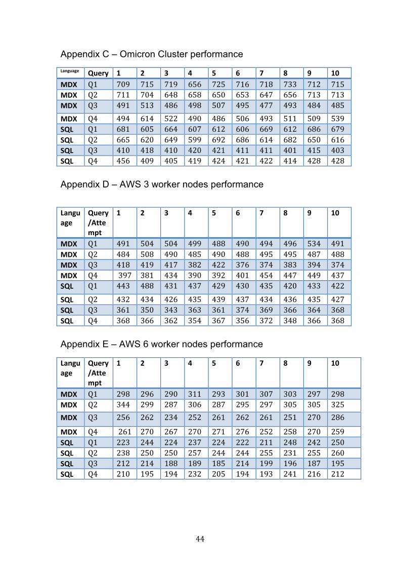
AppendixC–OmicronClusterperformance...................................................................44AppendixD–AWS3workernodesperformance........................................................44AppendixE–AWS6workernodesperformance.........................................................44AppendixF–AWS15workernodesperformance......................................................45AppendixG–SystemBenchmark........................................................................................45

viii

1

Abbreviations BI=BusinessIntelligence

CDE=CommunityDashboardEditor

CPU=CentralProcessorUnit

DAG=DirectedAcyclicGraph

GB=Gigabyte

GiB=Gibibyte

HDFS=HadoopDistributedFileSystem

HOLAP=HybridOLAP

I/O=InputOutput

JDBC=JavaDatabaseConnectivity

JNDI=JavaNamingandDirectoryInterface

JVM=JavaVirtualMachine

kB=Kilobyte

MB=Megabyte

MDX=MultiDimensionaleXpressions

MOLAP=MultidimensionalOLAP

OLAP=On-LineAnalyticalProcessing

OLTP=On-LineTransactionProcessing

RAM=Random-accessmemory

RDD=ResilientDistributedDataset

ROLAP=RelationalOLAP

SSB=StarSchemaBenchmark

SQL=StructuredQueryLanguage

YARN=YetAnotherResourceNegotiator

2

3

1. Introduction Due to the advances in technology, the amount of data being produced and

stored is continuously increasing. However, computers do not have the same

increase in performance and are not able to keep up. A way to tackle this

problem is to use multiple computers to process data in parallel, instead of

relyingontheperformanceofonecomputer.

TheBigDataconceptishardtodefine,butonedefinitioncanbeseenasadataset

that only can meet the service level agreements with the use of multiple

computerstohandleandstorethedata.Thismeansthattheconceptdependson

the context,making thedefinitionhard tograsp. (Wadkar, S., Siddalingaiah,M.

andVenner, J., 2014). The challengewith handlingBigData is not only that it

comesinlargevolume,butalsothatthedataoftenhasdifferentstructures,that

thepaceofthedataflowisfastandcontinuousandbecausethereoftenisbias

andnoiseinthedata.Thesecharacteristicscanbesummarizedusingthewords

Volume,Variety,VelocityandVeracityandarecalledthefourV’sofBigData.

ApacheHadoop is themostwellknownBigDataTechnologyPlatformand isa

framework that process large data amounts in parallel. Hadoop consist of an

entire ecosystem of components and most of them are open source projects

developed under Apache Software Foundations. A few examples of these

components or frameworks are Hadoop Distributed File System (HDFS), Map

Reduce, Apache Hive, Apache Spark and Apache Kylin (Mazumder, S., 2016).

AmazonWeb Services is a cloud service that provides Hadoop clusterswhere

users can specify how many resources that are of interest and allocate them

throughthecloud(Wadkar,S.,Siddalingaiah,M.andVenner,J.,2014).

OLAP is anumbrella term for techniquesused for analysingdatabases in real-

time.Thepurposeofthemethodisusuallytofindvaluableinsightsinthedata,

like trends or unexpected data, and is often usedwithin Business intelligence.

(Ordonez,C.,Chen,Z.andGarcía-García,J.,2011).OLAPusesadatamodelcalled

multidimensional database that stores aggregated data and creates a simpler

representationofthedata.Thisincreasestheperformanceofanalysingthedata

4

and alsomakes it easier tomaintain and understand. A way to represent the

multidimensionaldatabaseiswiththeuseofOLAPcubesthatorganisesthedata

intoa fact tableandmultipledimensions (Cuzzocrea,A.,Moussa,R.andXu,G.,

2013).Therearedifferentschematypesthatcanbeused formultidimensional

databases.The star schema is onemodel that is oftenused indatawarehouse

applications(deAlbuquerqueFilhoetal.2013).

SSB isabenchmark thathasbeencreated tomeasure theperformanceofdata

warehousesystems.Italsoprovidesgeneratorthatallowstheusertogeneratea

databaseinstarschemaformat.Thesizeofthegenerateddatabasedependsona

scalingfactorspecifiedbytheuser(deAlbuquerqueFilhoetal.2013).

TocreateandhandleanOLAPcube,anopensourceservercalledMondriancan

be used. It is integrated into the BI software Pentaho and uses the query

language MDX to send queries to a relational database. However, the ad-hoc

queriesusedinBIareusuallycomplexandifthecubeislarge,itwillrequirealot

of computational power. To increase the performance of the analysis, parallel

processing and distributed file systems can be used (Cuzzocrea, A.,Moussa, R.

andXu,G.,2013).

1.1 Purpose

This thesis investigates theanalysisof ad-hocqueriesonOLAPcubeswith the

useofApacheSparkonaHadoopcluster.Thegoalhasbeentoexaminewhether

Spark issuitable foranalysisofOLAPcubesandwhatperformancethatcanbe

expected.

Thisworkwillmainlybeperformedonaclusterconsistingof6nodeslocatedin

theOmicronCetioffice.However,tobeabletoseehowtheperformancescales

with the amount of nodes, clusters of different size created on Amazon Web

Services will also be used. The Star Schema Benchmark will be used for

generatingadatabasewithmorethanabillionrows.

5

Tohandlethecube,MondrianintegratedintoPentahoistobeused.Pentahoalso

haveaCommunityDashboardEditor(CDE)(Pentaho,2017)thatwillbeusedfor

sending MDX queries to Mondrian and to visualise the results. To be able to

comparehowtheBIserveraffectstheperformance,thesamequeriesinSQLwill

alsobesentstraight to thedatabaseonthecluster.Furthermore,ApacheKylin

willbeexaminedandtestedforOLAPcubeanalysis.

6

2. Theory

2.1 The Hadoop Ecosystem

HadoopisoneofthemostpopularBigDataplatformsusedtoday.Itisanopen-

source software that has been developed since 2002 and enables storing and

processingofBigDatainadistributedmanner(Huang,J.,Zhang,X.andSchwan,

K.,2015).Thefact that it isdistributedmeansthatHadoopisusedonmultiple

nodesinacluster.HadoopconsistsofanumberofcomponentswhereHDFSand

MapReduceare themain frameworksused for storingandprocessing thedata

(Mazumder,S.,2016).

2.1.1 HDFS HDFS is a distributed file system and stores the data on several nodes in the

cluster.Inalargeclusterwithalargeamountofnodes,somenodeswillfailevery

nowandthen.However,HDFSpreventsdatabeinglostbyreplicatingthedataon

multiplenodes.Whena file isuploaded toHDFS, the file is split intoblocksof

data.ThisisdoneusingslavecomponentscalledDataNodesthatcreatesblocks,

replicatesthemandstoresthem.ForHDFStokeeptrackofwhatdataisstored

where,amastercomponentcalledNameNodeisused.Thereisusuallyonlyone

NameNode in a Hadoop cluster while there are multiple DataNodes getting

instructionsfromtheNameNode(Vohra,Deepak,2016).

2.1.2 YARN YARN,orMapReduce2,isaframeworkintheHadoopecosystemthathandlesthe

distributedprocessingofthedata.SinceHDFSandYARNrunonthesamenodes,

thetaskstoberuncanbescheduledasefficientlyaspossible.Thismeansthata

taskisrunonthesamenodewherethedatatobeusedisstored(Vohra,Deepak,

2016;ApacheHadoop,ApacheHadoopYARN,2017).

TherearetwocomponentsinYARNthathandlestheresourceallocationandthat

istheResourceManagerandtheNodeManager.Alltypesofapplicationssentto

Hadoop will be allocated a resource for processing. The ResourceManager

7

runningonthemasternodewillschedulethisallocation.Eachslavenoderunsa

NodeManager that communicates with the ResourceManager and launches

containers and monitors their status. A container is a specified amount of

resourcesthatisallocatedontheclusterintermsofmemoryandvirtualcores.

TheamountofresourcesinacontainercandifferandaNodeManagercanhave

morethanonecontainer(Vohra,Deepak,2016;ApacheHadoop,ApacheHadoop

YARN,2017).

When an application is sent to Hadoop, the ResourceManager will, via the

NodeManager, create a container to run an ApplicationMaster. The

ApplicationMasterisaslavedaemonandwillmanageandlaunchthetasksinthe

application. ItnegotiateswiththeResourceManagerforresourcesandwiththe

NodeManagerforexecutionoftasks.Whenthetaskhasfinished,thecontainers

aredeallocatedandcanbeusedforrunninganothertask(Vohra,Deepak,2016;

ApacheHadoop,ApacheHadoopYARN,2017).

2.1.3 MapReduce MapandReducetaskaretwotypesoftasksthatcanberunonYARNtoprocess

data in parallel. TheMap interface represents the data as key/value pairs and

performsscalartransformationsonthem.AftergroupingtheresultfromMapby

thedifferentkeys,anarrayofallvaluesassociatedwitheachkeyiscreatedand

sent to the Reduce interface. Reduce finally applies some operations on each

arrayand returns the results (Mazumder, S., 2016).Anapplication that counts

the amount of words in a text file can be seen as an example to get a better

understandingofhowtheprocessworks.Multiplemapperswillgo throughall

the words in the text file and give each word a key-value pair in this way:

<<word>,1>.Allthepairsarethengroupedsothatifawordisfoundtwotimes

inatext,theyareputintothesamekey-valuepair.Forexample, ifawordwas

found2timesinatext,thekey-pairwouldbe:<<word>,2>.Theresultsfromall

mappers are then sent to the reducer that sums the values for all the words

foundinallmappers(ApacheHadoop,2017,Mapreducetutorial).

AfewexamplesofcomponentsthatcanrunonHDFSwiththeuseofYARNapart

fromMapReduce are Spark, Flink and Storm.When data comes in streams, in

8

Real Time orwhen iterative processing is needed,MapReduce is not suitable

(Mazumder,S.,2016).ThisisbecauseMapReducehastoreadandwritefromthe

disk between every job. Instead, Spark that stores the intermediate data in

memorycanbeused(Zaharia,M.etal.2010).

2.2 Apache Spark

Spark is a Distributed Processing Engine that stores the data sets in-memory,

whichiscalledResilientDistributedDataset(RDD).Thismeansthatthememory

oftheclusterisusedinsteadofbeingdependentofthedistributedfilesystem.In

addition,thedistributionofdataandtheparallelisationofoperationsaremade

automatically making Spark both easier to use and faster than MapReduce.

However,thefaulttoleranceandthelinearscalabilityforthetwoframeworksis

the same. Spark core is the heart of Spark and makes the in-memory cluster

computingpossible.ItcanbeprogrammedthroughtheRDDAPI,whichcomesin

multiplelanguagessuchasScala,Java,PythonandR(Salloum,S.etal.2016).

An RDD consists of data that is divided into chunks called partitions. Spark

performs a collection of computations on the cluster and then returns the

results.ThesecomputationsarealsoknownasjobsandaSparkapplicationcan

launchseveralofthem.ThejobisfirstsplitintoDAGs,whichconsistsofdifferent

stagesbuiltofasetoftasks.Thetasksareparalleloperationsandtherearetwo

types of them called transformations and actions. Transformation operations

definenewRDDsandaredeterministicand lazilyevaluated,whichmeans that

they wont be computed before an action operation is called. There are two

differenttypesoftransformationscallednarrowandwidetransformations.Ina

narrowtransformation,eachpartitionofthechildRDDonlyusesonepartitionof

theparentRDD.Mapandfilteraretwoexamplesofnarrowtransformations.Ina

widetransformationontheotherhand,severalpartitionsof thechildRDDuse

the same partition of the parent RDD. This means that wide transformations

needs data to be shuffled across the clusterwhich can be expensive since the

data needs to be sorted and partioned again. Two examples of wide

transformations are join and groupByKey. When data is shuffled in a wide

9

transformation, a new stage is started since all previous tasks need to be

completedbeforestartingtheshuffle.Actionsareoperationsthatreturnaresult

and are therefore found in the end of each job.When the action operation is

called, all transformations are first executed, and then the action. Three

examplesofactionoperationsarecount,firstandtake.Asstatedabove,eachjob

isdividedintostages.Theamountoftasksineachstagedependsonwhattypeof

operationsthatarepresentinthejob.(Salloum,S.etal.2016).Foreachpartition

of theRDD,a task iscreatedandthensent toaworkernode(Zaharia,M.etal.

2010).

Whenanapplication is run in Spark, five entities, namely a clustermanager, a

driver program, workers, executors and tasks, are needed. A cluster manager

allocatesresourcesoverthedifferentapplications(Salloum,S.etal.2016).Spark

StandAloneandYARNaretwotypesofclustermanagers(ApacheSpark,2017).

The driver program access Spark through a connection called SparkContext,

which connects the driver programwith the cluster. Theworker provides the

applicationwithCPU,storageandmemoryandeachworkerhasa JVMprocess

createdfortheapplicationcalledtheExecutor.Thesmallestunitsofworkthatan

executorisgivenaretasksandwhentheactionoperationisexecuted,theresults

arereturnedtothedriverprogram(Salloum,S.etal.2016).

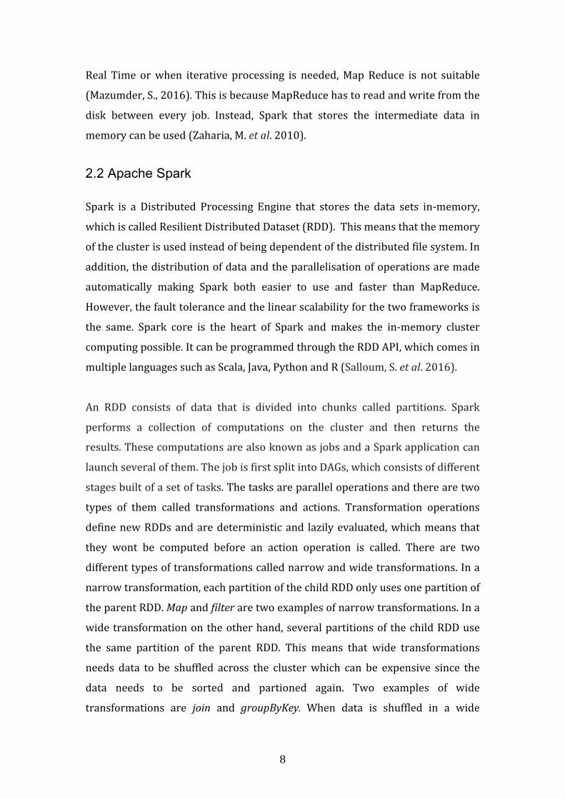
AnoverviewofhowYARNworkswithSparkandtwoworkernodescanbeseen

infigure1.

10

Figure1–ShowstheoverviewofaclusterusingYARNasaclustermanagerandtwoworkernodes.Inspiredbyfigure1inApacheSpark,ClusterModeOverview.

SparkSQL is a library that can be built on top of Spark core and is used for

processing structureddatausingSQL.This structureddata can forexamplebe

stored in a database, parquet files, CSV files or ORC files (Guller, M., 2015).

HadoophasasimilarprojectcalledApacheHive,whichtransformsSQLqueries

intoHadoopMapReducejobs(Lakhe,B.,2016).

2.3 Apache Hive

ApacheHiveisasystemusedfordatawarehousinginHadoop.ItusesanSQLlike

languagecalledHiveQLtocreatedatabasesandsendqueriesthataretranslated

into MapReduce jobs. Hive has a system catalog called Metastore where the

metadataofHivetablesarestoredinarelationaldatabasemanagementsystem.

TheseHive tablesaresimilar to tablesused in relationaldatabasesandcanbe

eitherinternalorexternal.Thedifferenceisthattheexternaltablewillhavedata

storedinHDFSorsomeotherdirectory,whiletheinternaltablestoresthedata

inthewarehouse.Thismeansthatthedatainaninternaltablewillbelostifthe

table is dropped, while the data in an external table still will be stored in its

original place if the table is dropped (Thusoo, A. et al. 2009). There are two

11

interfacestointeractwithHiveandthesearetheCommandLineInterface(CLI)

and HiveServer2. Hiveserver2 has a JDBC client called Beeline that is

recommendedtobeusedforconnectingtoHivebyHortonworks.(Hortonworks,

2017,ComparingBeelinetoHiveCLI).

SparkSQLcanalsobeusedwithBeeline forsendingqueries toHivetablesbut

usesaSparkengineinsteadofaHiveengine.Furthermore,aSparkJDBC/ODBC

servercanbeusedforsendingqueriesfromforexampleaBItooltoSparkthat

thensendthequeriestotheHivetables(Guller,M.,2015).

2.4 OLAP

Inmanybusinesses,On-LineTransactionProcessing(OLTP)databasesareused

forstoringinformationabouttransactions,employeedataanddailyoperations.

OLTP databases are relational databases and usually contain large amounts of

tableswithcomplexrelations. ThismakesOLTPdatabasesoptimal for storing

dataandaccuratelyrecordtransactionsandsimilar.However,tryingtoretrieve

andanalyse thisdatawill takea lotof timeandbecomputationallyexpensive.

An alternative to OLTP databases is using an Online Analytical Processing

(OLAP)database,whichextractsdata from theOLTPdatabaseand isdesigned

foranalysingdata.TheOLAPdatabaseisoftencreatedfromhistoricaldatasince

analysis of a constantly changing database is difficult (Microsoft Developer

Network, 2002).

2.4.1 Star schemas and Snowflake schemas TheschemastructureofanOLAPdatabasedifferstotheschemausedinanOLTP

database.There are two types of schemas that are commonlyusedwithOLAP

cubes, and these are called star schemas and snowflake schemas. They both

consists of multiple dimension tables, a fact table and measure attributes.

However,thesnowflakeschemaisamorecomplex,normalisedversionofastar

schema. The reason for this is because the snowflake schemahas a hierarchal

relational structure while the star schema has a flat relational structure. This

meansthatinastarschema,thefacttableisdirectlyjoinedtoallthedimensions,

12

while the snowflake schema has dimensions that are only joined to other

dimensions(Yaghmaie,M.,Bertossi,L.andAriyan,S.,2012).

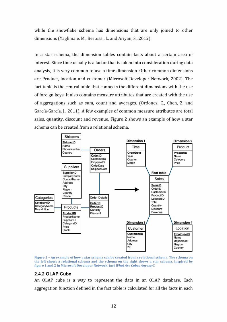
In a star schema, the dimension tables contain facts about a certain area of

interest.Sincetimeusuallyisafactorthatistakenintoconsiderationduringdata

analysis,itisverycommontouseatimedimension.Othercommondimensions

are Product, location and customer (Microsoft DeveloperNetwork, 2002). The

facttableisthecentraltablethatconnectsthedifferentdimensionswiththeuse

offoreignkeys.Italsocontainsmeasureattributesthatarecreatedwiththeuse

of aggregations such as sum, count and averages. (Ordonez, C., Chen, Z. and

García-García,J.,2011).Afewexamplesofcommonmeasureattributesaretotal

sales,quantity,discountandrevenue.Figure2showsanexampleofhowastar

schemacanbecreatedfromarelationalschema.

Figure2–Anexampleofhowastarschemacanbecreatedfromarelationalschema.Theschemaonthe left shows a relational schemaand the schemaon the right shows a star schema. Inspiredbyfigure1and2inMicrosoftDeveloperNetwork,JustWhatAreCubesAnyway?.

2.4.2 OLAP Cube An OLAP cube is a way to represent the data in an OLAP database. Each

aggregationfunctiondefinedinthefacttableiscalculatedforallthefactsineach

13

dimension.Forsimplicity,considerastarschemacontainingonlyonemeasure

attribute:totalsales,andthreedimensions:Date,ProductandLocation.Thecube

willthencalculatethetotalamountofsalesforeachdate,locationandproduct.

(MicrosoftDeveloperNetwork,2002).

TherearethreedifferenttypesofOLAPenginescalled:multidimensionalOLAP

(MOLAP),relationalOLAP(ROLAP)andHybridOLAP(HOLAP).MOLAPcreates

apre-computedOLAPcubefromthedatainadatabasethatitsendsqueriesto,

whileROLAPusesthedatastoredinarelationaldatabase.AHOLAPalsocreates

a cube but if it is needed, it can send queries straight to the database aswell

(Kaser,O.andLemire,D.,2006).

2.5 Mondrian

MondrianisaROLAPengineusedforhandlingandanalysingOLAPcubes.Torun

theengine,aserverisneededandthemostpopularbusinessanalyticsserveris

Pentaho.TobeabletomakeananalysisusingMondrian,aschemadefiningthe

OLAP cube is required as well as a JDCB connection to a relational database.

Mondrian uses the query languageMDX that it transforms into simplified SQL

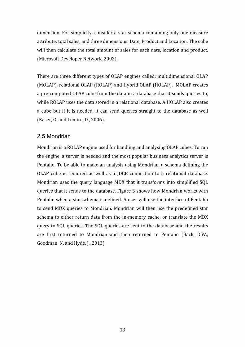
queriesthatitsendstothedatabase.Figure3showshowMondrianworkswith

Pentahowhenastarschemaisdefined.AuserwillusetheinterfaceofPentaho

to sendMDXqueries toMondrian.Mondrianwill thenuse thepredefined star

schema to either returndata from the in-memory cache, or translate theMDX

querytoSQLqueries.TheSQLqueriesaresenttothedatabaseandtheresults

are first returned to Mondrian and then returned to Pentaho (Back, D.W.,

Goodman,N.andHyde,J.,2013).

14

Figure 3 – Shows an example of how the connection between Pentaho, Mondrian and the datawarehouseworks. Inspiredby figure1.9 inMondrian InAction –Open sourcebusiness analytics,p.19.

2.6 OLAP on Hadoop

ThereareseveraloptionsforcreatingOLAPcubesinHadoopwithoutusingany

BI-tools.AfewexamplesareApacheLens(ApacheLens,2016),Druid,Atscale,

KyvosandApacheKylin(Hortonworks,2015,OLAPinHadoop).

2.6.1 Apache Kylin ApacheKylinisanopensourcetoolwithanSQLinterfacethatenablesanalysis

ofOLAPcubesonHadoop.KylinprebuildsMOLAPcubeswheretheaggregations

foralldimensionsarepre-computedandstored.ThisdataisstoredintoApache

HBasealongwithpre-joins that connect the factanddimension tables.Apache

HBase isanon-relationaldatabasethatcanberunontopofHDFS.If thereare

queries that cannot be sent to the cube,Kylinwill send them to the relational

databaseinstead.ThismakesKylinaHOLAPengine.Kylincreatesthecubefrom

datainaHivetable,andthenperformMapReducejobstobuildthecube(Lakhe,

B., 2016). In the latest version of Kylin, Spark can be used for creating of the

cube.However,theSparkengineiscurrentlyonlyaBetaversion(ApacheKylin,

2017.BuildCubewithSpark(beta)).

2.7 SSB benchmark

SSB consists of a number of ad-hoc queries that is meant for measuring the

performanceofadatabasebuiltofdatainstarschemaformat.Itisbasedonthe

15

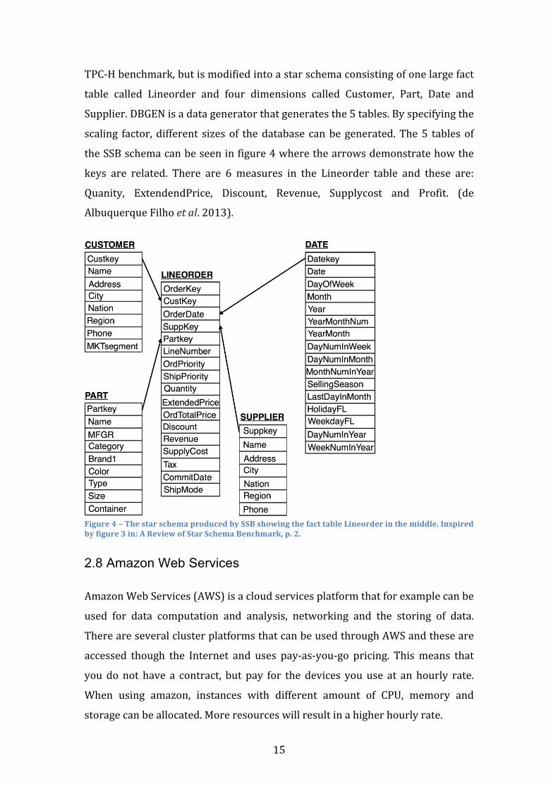
TPC-Hbenchmark,butismodifiedintoastarschemaconsistingofonelargefact

table called Lineorder and four dimensions called Customer, Part, Date and

Supplier.DBGENisadatageneratorthatgeneratesthe5tables.Byspecifyingthe

scaling factor,different sizesof thedatabase canbegenerated.The5 tablesof

theSSBschemacanbeseeninfigure4wherethearrowsdemonstratehowthe

keys are related. There are 6 measures in the Lineorder table and these are:

Quanity, ExtendendPrice, Discount, Revenue, Supplycost and Profit. (de

AlbuquerqueFilhoetal.2013).

Figure4–ThestarschemaproducedbySSBshowingthefacttableLineorderinthemiddle.Inspiredbyfigure3in:AReviewofStarSchemaBenchmark,p.2.

2.8 Amazon Web Services

AmazonWebServices(AWS)isacloudservicesplatformthatforexamplecanbe

used for data computation and analysis, networking and the storing of data.

ThereareseveralclusterplatformsthatcanbeusedthroughAWSandtheseare

accessed though the Internet and uses pay-as-you-go pricing. Thismeans that

youdo not have a contract, but pay for the devices you use at an hourly rate.

When using amazon, instances with different amount of CPU, memory and

storagecanbeallocated.Moreresourceswillresultinahigherhourlyrate.

16

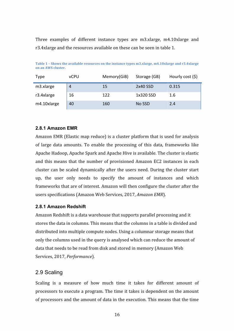
Three examples of different instance types are m3.xlarge, m4.10xlarge and

r3.4xlargeandtheresourcesavailableonthesecanbeseenintable1.

Table1–Showstheavailableresourcesontheinstancetypesm3.xlarge,m4.10xlargeandr3.4xlargeonanAWScluster.

Type vCPU Memory(GiB) Storage(GB) Hourlycost($)

m3.xlarge 4 15 2x40SSD 0.315

r3.4xlarge 16 122 1x320SSD 1.6

m4.10xlarge 40 160 NoSSD 2.4

2.8.1 Amazon EMR

AmazonEMR(Elasticmapreduce)isaclusterplatformthatisusedforanalysis

of large data amounts. To enable the processing of this data, frameworks like

ApacheHadoop,ApacheSparkandApacheHiveisavailable.Theclusteriselastic

and thismeans that thenumberofprovisionedAmazonEC2 instances in each

clustercanbescaleddynamicallyafter theusersneed.During theclusterstart

up, the user only needs to specify the amount of instances and which

frameworksthatareofinterest.Amazonwillthenconfiguretheclusterafterthe

usersspecifications(AmazonWebServices,2017,AmazonEMR).

2.8.1 Amazon Redshift

AmazonRedshiftisadatawarehousethatsupportsparallelprocessingandit

storesthedataincolumns.Thismeansthatthecolumnsinatableisdividedand

distributedintomultiplecomputenodes.Usingacolumnarstoragemeansthat

onlythecolumnsusedinthequeryisanalysedwhichcanreducetheamountof

datathatneedstobereadfromdiskandstoredinmemory(AmazonWeb

Services,2017,Performance).

2.9 Scaling

Scaling is a measure of how much time it takes for different amount of

processorstoexecuteaprogram.Thetimeittakesisdependentontheamount

ofprocessorsandtheamountofdataintheexecution.Thismeansthatthetime

17

canbeseenasafunction:𝑇𝑖𝑚𝑒 𝑝, 𝑥 wherepistheamountofprocessorsandx

thesizeoftheproblem.Measuringthetimeittakesforoneprocessorcompared

to multiple processors to execute a problem of a fixed size is called strong

scaling.Speedupisameasureofhowmuchaproblemisoptimisedafteradding

moreprocessors.Thespeedupcanbemeasuredintermsofstrongscalingandit

canbeseeninformula1.Justasstatedabove,pistheamountofprocessorsand

xthesizeoftheproblem.

𝑠𝑝𝑒𝑒𝑑𝑢𝑝 𝑝, 𝑥 =𝑡𝑖𝑚𝑒 1, 𝑥𝑡𝑖𝑚𝑒 𝑝, 𝑥 (1)

Theidealscalingpatternforstrongscalingisalineargraphwhenthenumbersof

processorsareplottedagainstthespeedup.Thismeansthatthespeedupdivided

withtheamountsofnodesshouldbecloseto1inidealscalingandthisismore

knownaslinearscaling(Kim,M.,2012).

Anotherway to estimatehowa systemscales is to look at the throughputper

node.Thethroughputistheamountofdatabeingprocessedpertimeunit.Ifthe

throughput is measured in Mb/second, then dividing this with the amount of

nodes used for the execution results in Mb/(second*node). If a system has

perfect linear scaling, then the throughput per node should be the same for

queriesranondifferentamountofnodes(Schwartz,B.,2015).

However, Gene Amdahl means that this perfect scaling cannot always be

expected.HeproposedalawcalledAmdahlsLawthatstatesthataproblemhas

twoparts:one that isoptimisableandone that isnon-optimisable.Thismeans

that he claims that there is a fraction of a problem thatwont get a decreased

executiontime,regardlessoftheamountofprocessorsinvolved(Kim,M.,2012).

2.10 Previous work

The SSB benchmark has been used and studied with Spark before. Benedikt

Kämpgen and AndreasHarth that translated the SSB benchmark queries from

SQLtoMDXintheirarticlecalledNosizeFitsAllisoneexample.Theycompared

theperformanceoftheSSBbenchmarkusingbothSQLandMDXwithMondrian

18

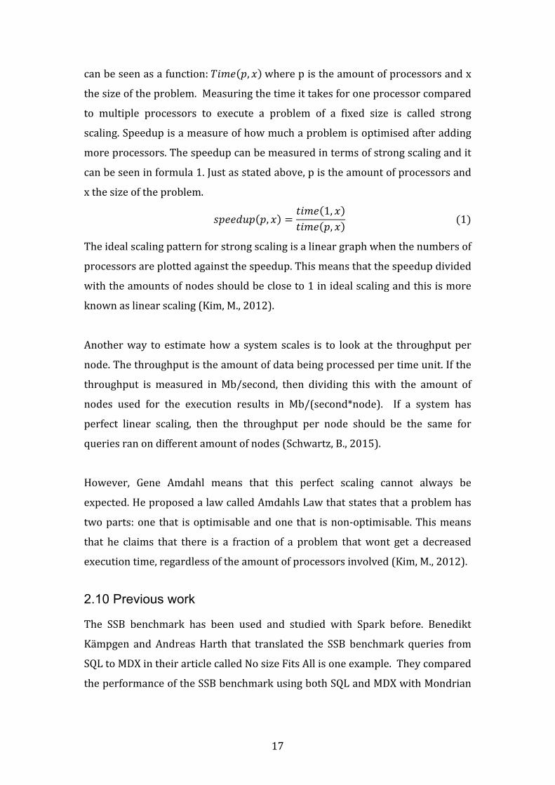
justlikeinthisthesis.Theresultsthattheyobtainedforeachquerycanbeseen

intable2.

Table2–ShowshowtheresultsthatBenediktKämpgenandAndreasHarthobtainedinthearticleNosizeFitsAll.

Language Q1 Q2 Q3 Q4

MDX 14.7s 14.5s 5.1s 4.8s

SQL 15.47s 15.4s 5.3s 5.0s

ThedatabasewasintheircasestoredinaMySQLdatabaseandthedatabaseonly

consistedofaround6millionrows.Aclusterwasnotusedeither,butacomputer

withaCPUof16coresand128GBRAM.

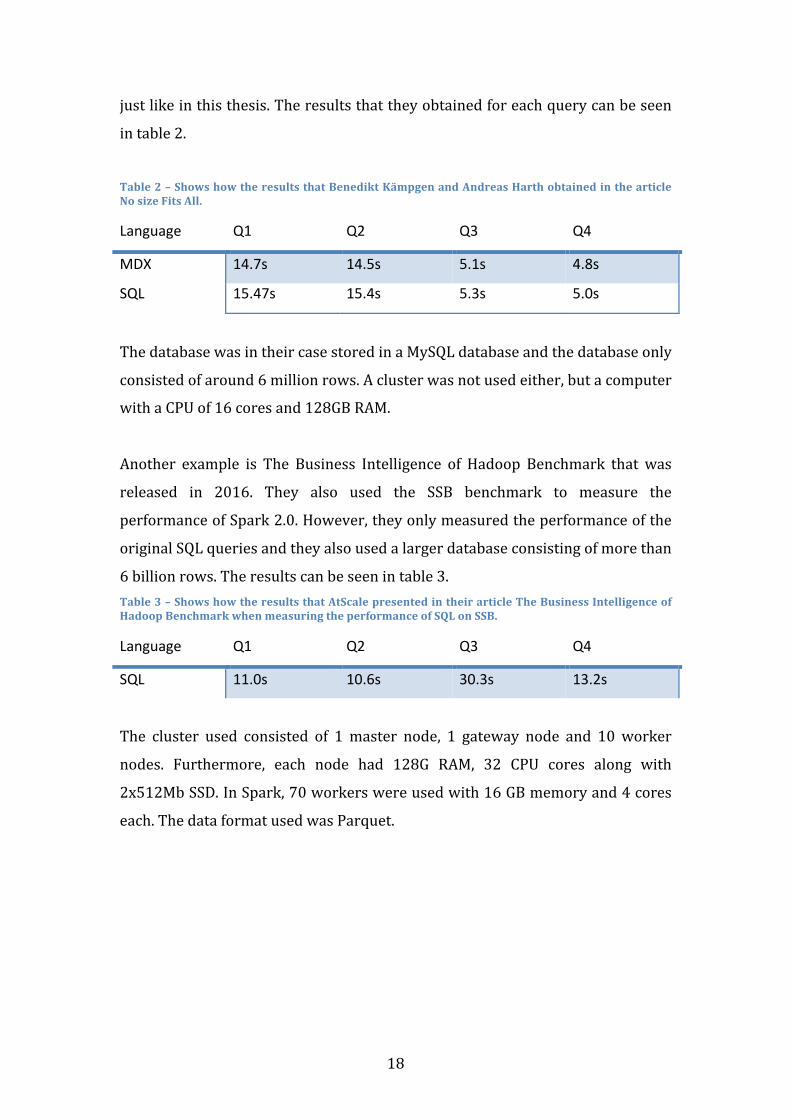
Another example is The Business Intelligence of Hadoop Benchmark that was

released in 2016. They also used the SSB benchmark to measure the

performanceofSpark2.0.However,theyonlymeasuredtheperformanceofthe

originalSQLqueriesandtheyalsousedalargerdatabaseconsistingofmorethan

6billionrows.Theresultscanbeseenintable3.Table3–ShowshowtheresultsthatAtScalepresentedintheirarticleTheBusinessIntelligenceofHadoopBenchmarkwhenmeasuringtheperformanceofSQLonSSB.

Language Q1 Q2 Q3 Q4

SQL 11.0s 10.6s 30.3s 13.2s

The cluster used consisted of 1 master node, 1 gateway node and 10 worker

nodes. Furthermore, each node had 128G RAM, 32 CPU cores along with

2x512MbSSD.InSpark,70workerswereusedwith16GBmemoryand4cores

each.ThedataformatusedwasParquet.

19

3. Method Anumberof implementationswereneeded inorder tobeable toestimate the

performance of ad-hoc queries on OLAP cubes with Spark. This included a

cluster with the right configurations, data to populate the database with, a

databaseonthecluster,anenginetohandletheOLAPcube,aninterfacewhere

queriesarespecifiedandaschemadefiningtheOLAPcube.Furthermore,Kylin

was implemented into Hadoop in order to try to create a ROLAP cube. Since

differenthardwarehasbeenusedonthedifferentclusters,asystembenchmark

wasrunonthemasternodeoftheclusters.

3.1 Cluster setup

Twodifferenttypesofclusterswereusedtoperformthework:aclusterlocated

intheOmicronCetiofficeandofficescreatedonAWS.Thepurposeofusingthe

AWSclusterwastobeabletocreateclustersofdifferentsize.Thisisbecauseby

measuringtheperformanceondifferentsizedclusters,itispossibletoestimate

thescalingoftheperformance.

3.1.1 The Omicron cluster The cluster in the Omicron Ceti office consists of 6 nodes where 1 node is a

masterandtheother5areworkernodes.TheRAMineachdatanodeis16GB

and4virtualCPUcores.Hadoopversion2.5.3.0andHiveversion1.2.1000have

beenused. The Spark versionused on the clusterwas version2.0.0.However,

whenrunningandKylin,Sparkwithversion1.6.3wasusedas theengine.The

versionofKylinwas2.0.0.

3.1.2 The AWS cluster TheclusterscreatedontheAWScloudconsistedof3differentsizes.Theclusters

allhadonemasternodebuthadadifferentamountofnamenodes.Thenumbers

of namenodes in the three clusterswere 3, 6 and 15. Every nodewas of size

m3.xlargemeaningthatthevirtualCPUhad4coresandthattheRAMwas15GB.

The software implemented on the clusters was Hadoop version 2.7.3, Hive

version2.1.0andSparkversion2.0.2.

20

3.2 Data

There are several benchmarks that previously have been used for testing the

performanceofdatawarehousessuchasTPC-H.However,thedatabaseusedin

theTPC-Hbenchmark isnot in star schema format,and isnot suitable for this

kind of analysis where OLAP cubes are used. Therefore, the Star Schema

benchmark (SSB),which has been developed from the TPC-H benchmark,was

usedinstead.

Itwasdecidedthatadatabaseofatleast1billionrowswasneededtobeableto

call thetaskaBigDataproblem. Therefore,thescalingfactor200wasusedto

create the database with SSB’s data generator DBGEN. This resulted in a fact

tableofmorethan1.2billionrows.Thegeneratorreturns5textfileswhereeach

filecontains the informationaboutaspecific table.Thesizeand theamountof

rowsofeachtablecanbeseenintable4.

Table4–Showsthefilesizeandtheamountofrowsineachofthetablescreatedwhenusingscalingfactor200

Table Filesize Rows

Lineorder 119GB 1200018603

Customer 554MB 6000000

Part 133MB 1600000

Supplier 33MB 400000

Dates 225kB 2556

Data files saved inparquet formatwill runbetterwithSparkSQL thannormal

text files. This is because parquet files use a compressed columnar storage

format(Ousterhout,K.etal.2015).Therefore,thetextfileswerealsoconverted

into parquet files and this took about 6 hours on the Omicron cluster. When

runningtheSQLqueriesonthedatabasecreatedfromtheparquetfilehowever,

the queries took about 2-3 times longer to run. Furthermore, since the AWS

cluster cost money every hour a cluster is up and running, it would bemore

expensive tocreateparquet files fromthegeneratedtext files. Itwas therefore

decidedtousetheoriginaltextfiles.

21

AproblemwithDBGENisthatitcreatesthedatafilesonthemasternode.This

meansthatthemasternodeneedstohavestoragefor120GB,whichwasnotthe

caseonthemasternodeontheAWScluster.Therefore,aDBGENthatcreatedthe

tables straight into HDFS usingMapReducewas used1. This created 5 folders,

one for each table, with all the output data divided into smaller part files on

HDFS.Allfileswerebydefaultcompressed,whichcausesproblemswhentrying

tocreateadatabase fromthedata.Thesettingswere thereforechanged in the

javacodesothatuncompressedtextfilesweresavedonHDFSinstead.

3.3 Queries

TheSSBbenchmarkqueriesconsistof13queries thatcanbedivided into four

blockswithdifferentselectivity.AllqueriesareoriginallyinSQLsyntax,buthave

been translated intoMDXqueriesbyBenediktKämpgenandAndreasHarth in

20132.

The queries were first run against the database on the local cluster and the

resultswere inspected.Unfortunately,Pentahocouldnothandlecastingvalues

as“numeric”andasyntaxerrorwasthereforereturnedwheneverthisoperation

wasused.TherewasalsooneMDXquerythatstarted“WITHMEMBER”instead

of“SELECT”whichisusuallyusedandalsoreturnedasyntaxerror.Twoqueries

didnotreturnanyresultsneitherwhenrunningitthroughPentahousingMDX,

norwhenusingSQLdirectlyonthedatabaseusingBeeline.

Thismeans thatonly fourof the13MDXqueriescouldbehandledbyPentaho

and returned results. Luckily, the queriesworking belonged to the blocks that

usedmediumandhighdatasetcomplexityandvolume.Allfourworkingqueries

can be found in both SQL and MDX syntax in Appendix A and B. In the SSB

1https://github.com/electrum/ssb-dbgen2http://people.aifb.kit.edu/bka/ssb-benchmark/

22

benchmark, these queries are called Q2.2, Q2.3, Q4.2 and Q4.3, but are for

simplicitycalledQ1,Q2,Q3andQ4here.

QueryQ1 andQ2make three JOIN operations, two GROUPBY operations and

twoFILTERoperations.However,Q2ismoreselectivethanQ1.QueryQ3andQ4

ontheotherhandmakesfourJOINoperations,threeGROUPBYoperationsand

threeFILTERS andQ4 ismore selective thanQ3 (Thebusiness intelligenceon

hadoopbenchmark,2016).

A database consisting of Hive tables was created with the use of Beeline. By

specifying which port that Beeline should connect to, Hive or Spark could be

usedastheengine.SinceittookmanyhourstoproducethetableswithDBGEN,

external tables were chosen so that the datawould not be dropped if a table

were. With Beeline, queries were easily sent to the database with SQL like

syntax.

3.5 Mondrian in Pentaho

It was already decided that the OLAP engine Mondrian was to be used for

creatingandhandlingtheOLAPcube.However,Mondriancannotrunaloneand

needs a server and in this case, the server Tomcat was used. Tomcat can be

either run in standalone mode, or integrated into other webservers. Tomcat

standalonewasfirstusedwithPivot4jastheJavaAPI.However,theresultsfrom

thequeries came in too large sizes and could thereforenot be representedby

Pivot4j. Therefore, Tomcat integrated into Pentaho was used. The Pentaho

serverwasrunningfrommypersonallaptop.

To be able to send queries from Pentaho to a cluster, a JDBC connection is

needed.SincetheideawastosendqueriestoSparkSQL,aSparkJDBCconnection

neededtobeused.However,thisconnectionwasnotworkinginPentaho.Toget

the connection towork, Pentaho’s data integration tool calledKettlewas used

sinceitissimplerthanPentahosplatformforanalysis.ASparkJDBCjarfile,14

23

otherjarfilesandalicencefileweredownloadedfromSimba3.However,forthe

connectiontobesuccessful,onlyfourofthese14jarsweretobeincludedinthe

setup.Thesefourjarswere:hive_service.jar,httpclient-4.13.jar,libthrift-0.9.0.jar

andtheTCLIServiceClient.jar.TheSparkJDBCjar,thelicencefileandthefourjar

filesspecifiedabovewereput intotwolibfolders inPentaho45.Sincethereisa

charge to use the full version of Simba’s JDBC connectors, a trial versionwas

used. The difference was that the licence file was only available for a month.

Therefore,anewlicencewassimplydownloadedwhenthe licenceranoutand

putinthetwolibfolders.Anotherconfigurationneededtoconnecttothecluster

wastosetactive.hadoop.configuration=hdp24intheplugin.propertiesfile6.

Aftermaking these configurations, the IP address of the cluster was specified

along with the connection port and the name of the database created on the

cluster.ThedefaultportforSparkis10015.Whentheconnectionwassuccessful,

theJDBCconnectionbecomesavailableunderdatasources.

ForMondrian tobeable tocreateanOLAPcube,anOLAPschemaneeds tobe

specified.ThisisdoneusinganXMLmetadatafilethatspecifiestheattributesin

thefacttableandthedimensions,theprimarykeysandthemeasures.However,

itwasnot possible to upload this file straight intoPentaho. Instead,Pentaho’s

Mondrian Schema Workbench was used to publish the cube into Pentaho.

BenediktKämpgenandAndreasHarthpresentanXMLschema2 that theyhave

usedtocreateanSSBOLAPschema.ThisXMLfilewasused,butmodifiedusing

SchemaWorkbenchso that itcorrespondedcompletely to theSSBdatabaseon

the cluster. After the schema was correctly specified, it was published to

Pentaho.Whenpublished,itappearedunderdatasourcesinPentaho.

3http://www.simba.com/product/spark-drivers-with-sql-connector/4pentaho-server/pentaho-solutions/system/kettle/plugins/pentaho-big-data-

plugin/hadoop-configurations/hdp24/lib/5pentaho-server/tomcat/webapps/pentaho/WEB-INF/lib/

6pentaho-server/pentaho-solutions/system/kettle/plugins/pentaho-big-data-plugin/plugin.properties

24

SincePivot4jcouldnotrepresenttheamountofdatareturnedbythequeries,the

Pentahotool“AnalysisReport”wastobeusedinstead.However,thisfeaturewas

onlyavailableontheenterpriseeditionofPentaho,andthecommunityedition

was the one running onmy laptop. Luckliy, Omicron had Pentaho running in

enterprise edition on an instance on AWS. TheMDX queries were run on the

AnalysisReporttool,butunfortunately,itcouldnotrepresenttheresultingdata

either.

CDEwasthetoolthatfinallymanagedtoreturnandrepresentthedataformthe

MDXqueries.WhenusingCDE,adatasourcetypeneedstobeselected,andhere,

“mdxovermondrianJndi”wasused. Since a JDBC connection alreadyhasbeen

created,onlyaJNDIconnectionisneededwheretheJDBCconnectionisselected

assource.AMondrianschemaalsoneedstobespecified,andtheonepublished

through Schema workbench was therefore used. The component chosen to

representthedatawasTable.Thismeansthattheresultsfromthequerieswere

representedinatable.

3.6 Running the queries

Each querywas run10 times in order to provide a consistent result. The SQL

queriesweresenttothedatabaseusingBeeline.TheMDXqueriesweresentto

thedatabasethroughPentaho’sCDE.InordertopreventPentahofromcaching,

the serverwas restarted between each run. Furthermore, the System Settings,

ReportingMetadata,GlobalVariables,MondrianSchemaCache,ReportingData

CacheandtheCDACachewerealsorefreshedbetweeneachrun.Thetimeittook

foreachquery to runwasobserved from theSparkApplicationmaster.There,

eachjobbeingexecutedwasshownalongwiththetimeittooktorunthem.

3.7 Kylin

ApacheKylinversion2.0wasdownloadedandinstalledonthemasternodeon

theOmicronCluster.TwodifferentsizedcubeswerethencreatedinKylinwith

allthedimensions, joins,andmeasurespresentinthedatabase.Thelargecube

was tobe created from theSSBdatabaseused in thebenchmarking.A smaller

cubewasalsotobemadefromanSSBdatabaseofaround6millionrows.Inthe

25

latestversionofKylin,theusercanbuildthecubeusingSparkastheengine.This

featureisatcurrenttimeonlyinBetaversion.

3.8 System benchmark

In order to compare performance the two cluster types properly and find

possible bottlenecks, a system benchmark was run. The benchmark is called

Sysbench and the performance of the CPU, reading and writing to RAM and

Input/Output(I/O)readingandwritingwasmeasured.Thecommandosusedfor

thebenchmarkcanbeseeninAppendixG.

26

4. Results EachqueryinSQLandMDXwasrun10timesandtheresultsfromeachruncan

beobservedinAppendixC,D,EandF.Inthefollowingsections,onlytheaverage

timeittooktorunthe10runsisshown.

Itwasnotedthat foreachquery,regardlessof language, the lastpartitiontook

muchlongertorunthantheotherpartitions.

4.1 The Omicron Cluster

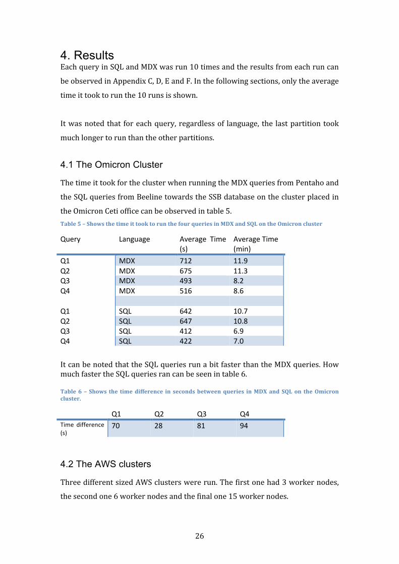
ThetimeittookfortheclusterwhenrunningtheMDXqueriesfromPentahoand

theSQLqueriesfromBeelinetowardstheSSBdatabaseontheclusterplacedin

theOmicronCetiofficecanbeobservedintable5.Table5–ShowsthetimeittooktorunthefourqueriesinMDXandSQLontheOmicroncluster

Query Language Average Time(s)

AverageTime(min)

Q1 MDX 712 11.9Q2 MDX 675 11.3Q3 MDX 493 8.2Q4 MDX 516 8.6 Q1 SQL 642 10.7Q2 SQL 647 10.8Q3 SQL 412 6.9Q4 SQL 422 7.0

ItcanbenotedthattheSQLqueriesrunabitfasterthantheMDXqueries.HowmuchfastertheSQLqueriesrancanbeseenintable6.Table6 – Shows the timedifference in secondsbetweenqueries inMDXandSQLon theOmicroncluster.

Q1 Q2 Q3 Q4Time difference(s)

70 28 81 94

4.2 The AWS clusters

ThreedifferentsizedAWSclusterswererun.Thefirstonehad3workernodes,

thesecondone6workernodesandthefinalone15workernodes.

27

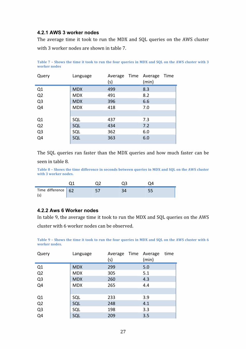
4.2.1 AWS 3 worker nodes The average time it took to run theMDX and SQLqueries on theAWS cluster

with3workernodesareshownintable7.

Table7–ShowsthetimeittooktorunthefourqueriesinMDXandSQLontheAWSclusterwith3workernodes


Average Time(min)


TheSQLqueries ran faster than theMDXqueriesandhowmuch faster canbe

seenintable8.Table8–ShowsthetimedifferenceinsecondsbetweenqueriesinMDXandSQLontheAWSclusterwith3workernodes.


62 57 34 55

4.2.2 Aws 6 Worker nodes Intable9,theaveragetimeittooktoruntheMDXandSQLqueriesontheAWS

clusterwith6workernodescanbeobserved.

Table9–ShowsthetimeittooktorunthefourqueriesinMDXandSQLontheAWSclusterwith6workernodes.


Average time(min)


28

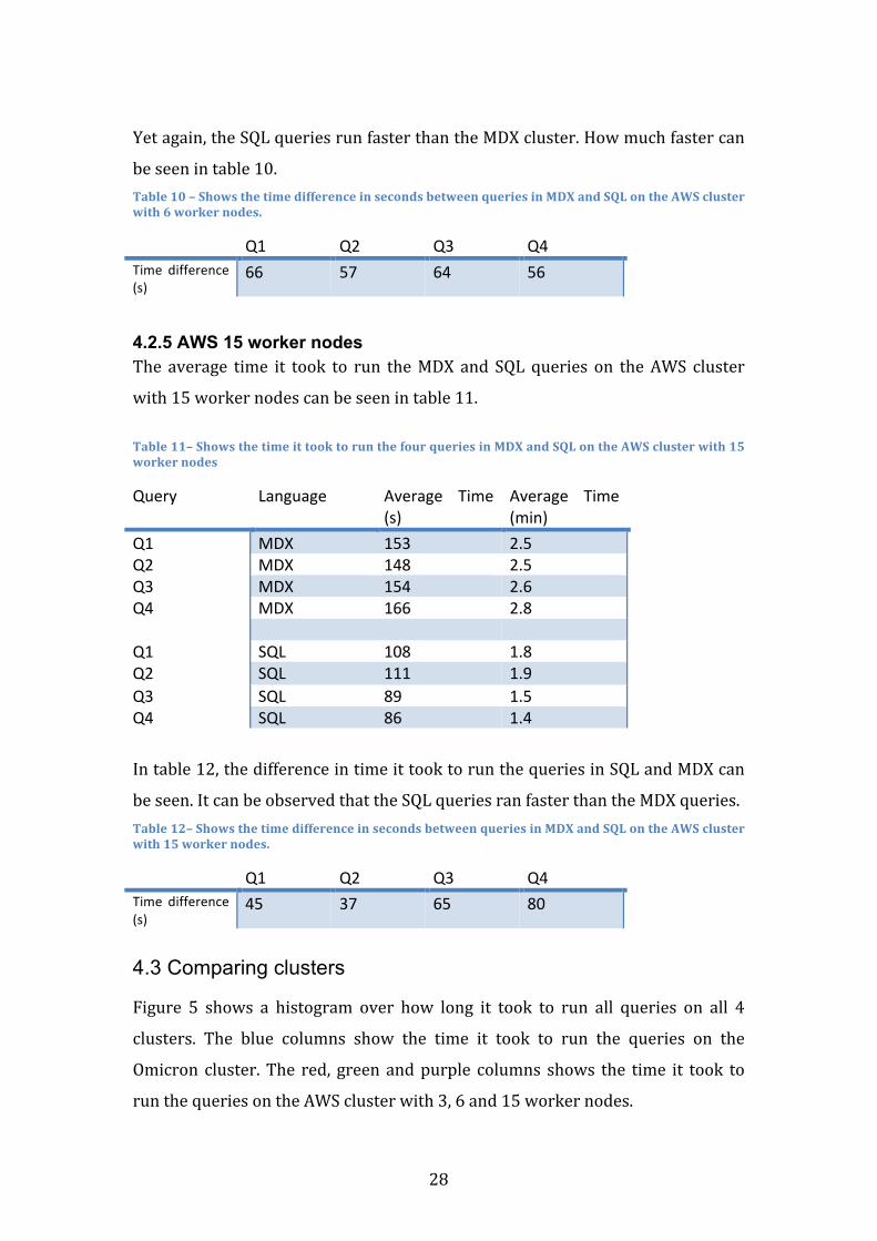
Yetagain,theSQLqueriesrunfasterthantheMDXcluster.Howmuchfastercan

beseenintable10.Table10–ShowsthetimedifferenceinsecondsbetweenqueriesinMDXandSQLontheAWSclusterwith6workernodes.


66 57 64 56

4.2.5 AWS 15 worker nodes The average time it took to run theMDX and SQLqueries on theAWS cluster

with15workernodescanbeseenintable11.

Table11–ShowsthetimeittooktorunthefourqueriesinMDXandSQLontheAWSclusterwith15workernodes


Average Time(min)


Intable12,thedifferenceintimeittooktorunthequeriesinSQLandMDXcan

beseen.ItcanbeobservedthattheSQLqueriesranfasterthantheMDXqueries.Table12–ShowsthetimedifferenceinsecondsbetweenqueriesinMDXandSQLontheAWSclusterwith15workernodes.


45 37 65 80

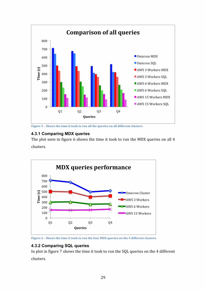
4.3 Comparing clusters

Figure 5 shows a histogram over how long it took to run all queries on all 4

clusters. The blue columns show the time it took to run the queries on the

Omicron cluster.The red, greenandpurple columns shows the time it took to

runthequeriesontheAWSclusterwith3,6and15workernodes.

29

Figure5–Showsthetimeittooktorunallthequeriesonalldifferentclusters.

4.3.1 Comparing MDX queries Theplotseeninfigure6showsthetimeittooktoruntheMDXqueriesonall4

clusters.

Figure6–ShowsthetimeittooktorunthefourMDXqueriesonthe4differentclusters.

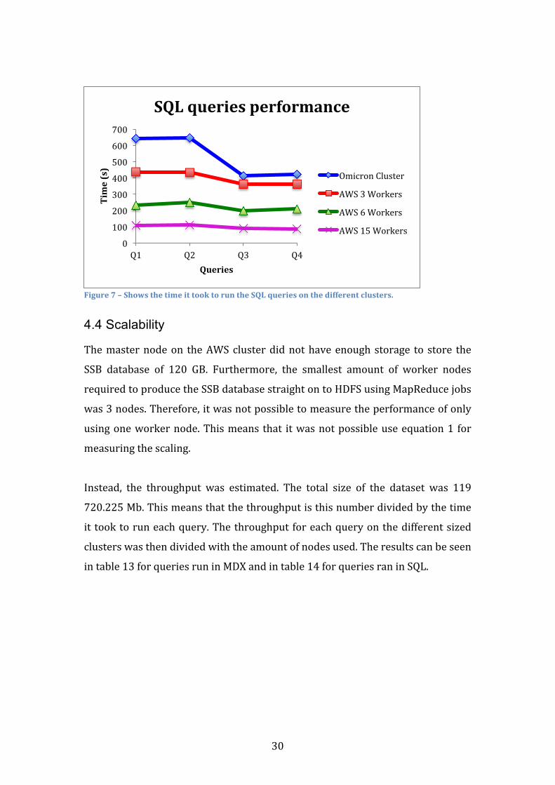
4.3.2 Comparing SQL queries Inplotinfigure7showsthetimeittooktoruntheSQLqueriesonthe4different

clusters.

0

100

200

300

400

500

600

700

800

Q1 Q2 Q3 Q4

TIme(s)

Queries

Comparisonofallqueries

OmicronMDX

OmicronSQL

AWS3WorkersMDX

AWS3WorkersSQL

AWS6WorkersMDX

AWS6WorkersSQL

AWS15WorkersMDX

AWS15WorkersSQL

0100200300400500600700800

Q1 Q2 Q3 Q4

Time(s)

Queries

MDXqueriesperformance

OmicronCluster

AWS3Workers

AWS6Workers

AWS15Workers

30

Figure7–ShowsthetimeittooktoruntheSQLqueriesonthedifferentclusters.

4.4 Scalability

Themasternodeon theAWSclusterdidnothaveenoughstorage to store the

SSB database of 120 GB. Furthermore, the smallest amount of worker nodes

requiredtoproducetheSSBdatabasestraightontoHDFSusingMapReducejobs

was3nodes.Therefore,itwasnotpossibletomeasuretheperformanceofonly

usingoneworkernode.Thismeans that itwasnotpossibleuseequation1 for

measuringthescaling.

Instead, the throughput was estimated. The total size of the dataset was 119

720.225Mb.Thismeansthatthethroughputisthisnumberdividedbythetime

ittooktoruneachquery.Thethroughputforeachqueryonthedifferentsized

clusterswasthendividedwiththeamountofnodesused.Theresultscanbeseen

intable13forqueriesruninMDXandintable14forqueriesraninSQL.

0

100

200

300

400

500

600

700

Q1 Q2 Q3 Q4

Time(s)

Queries

SQLqueriesperformance

OmicronCluster

AWS3Workers

AWS6Workers

AWS15Workers

31

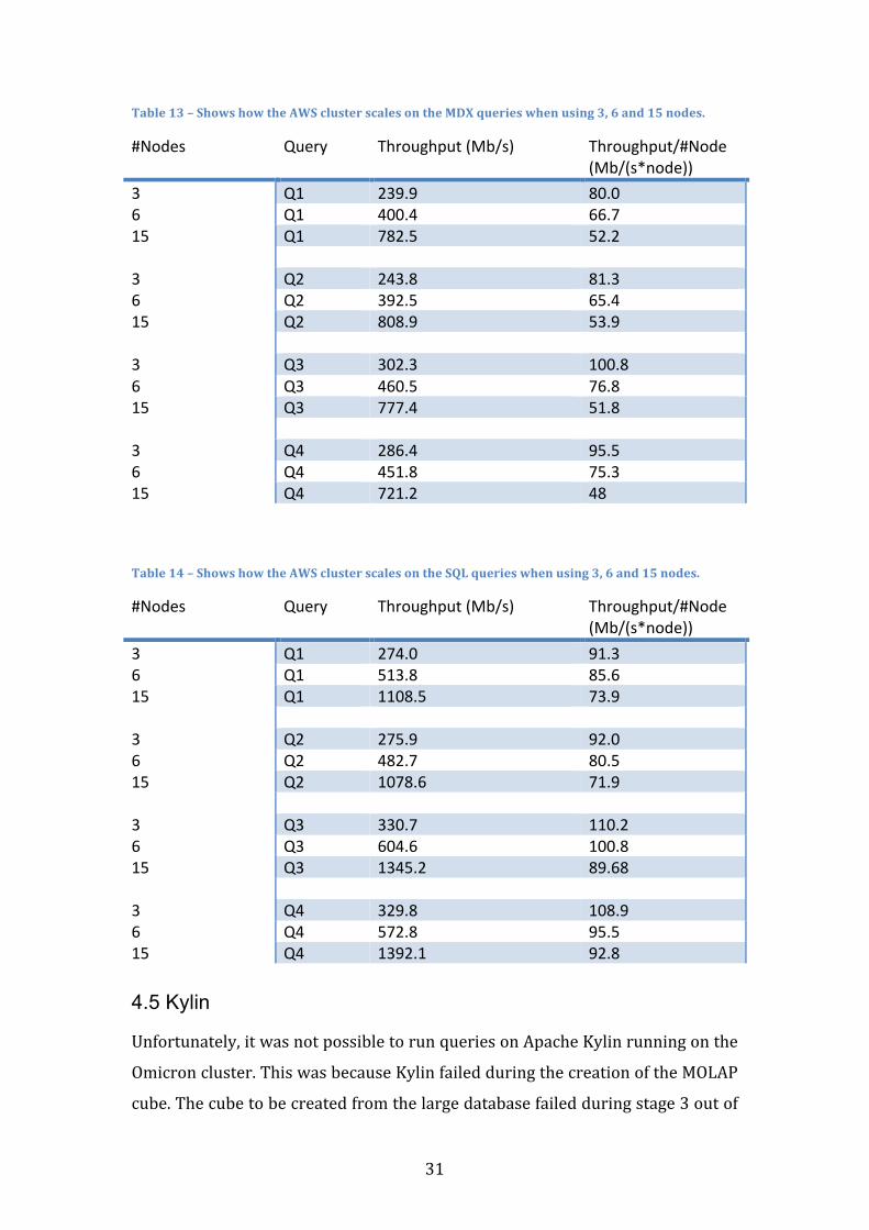
Table13–ShowshowtheAWSclusterscalesontheMDXquerieswhenusing3,6and15nodes.

#Nodes Query Throughput(Mb/s) Throughput/#Node(Mb/(s*node))

3 Q1 239.9 80.06 Q1 400.4 66.715 Q1 782.5 52.2 3 Q2 243.8 81.36 Q2 392.5 65.415 Q2 808.9 53.9 3 Q3 302.3 100.86 Q3 460.5 76.815 Q3 777.4 51.8 3 Q4 286.4 95.56 Q4 451.8 75.315 Q4 721.2 48Table14–ShowshowtheAWSclusterscalesontheSQLquerieswhenusing3,6and15nodes.

#Nodes Query Throughput(Mb/s) Throughput/#Node(Mb/(s*node))

3 Q1 274.0 91.36 Q1 513.8 85.615 Q1 1108.5 73.9 3 Q2 275.9 92.06 Q2 482.7 80.515 Q2 1078.6 71.9 3 Q3 330.7 110.26 Q3 604.6 100.815 Q3 1345.2 89.68 3 Q4 329.8 108.96 Q4 572.8 95.515 Q4 1392.1 92.8

4.5 Kylin

Unfortunately,itwasnotpossibletorunqueriesonApacheKylinrunningonthe

Omicroncluster.ThiswasbecauseKylinfailedduringthecreationoftheMOLAP

cube.Thecubetobecreatedfromthelargedatabasefailedduringstage3outof

32

the11stages.Thisstageextractsthedistinctcolumnsinthefacttableandfailed

because all the memory was used. The cube to be created from the smaller

databasemanaged torun tostage7whichbuilt thecubewithSpark.Thisalso

failedduetothesystembeingoutofmemory.

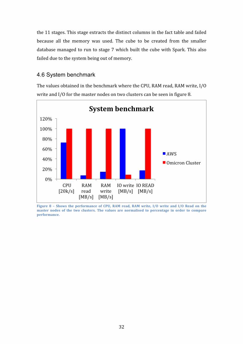
4.6 System benchmark

ThevaluesobtainedinthebenchmarkwheretheCPU,RAMread,RAMwrite,I/O

writeandI/Oforthemasternodesontwoclusterscanbeseeninfigure8.

Figure 8 – Shows the performance of CPU, RAM read, RAMwrite, I/Owrite and I/O Read on themaster nodes of the two clusters. The values are normalised to percentage in order to compareperformance.

0%

20%

40%

60%

80%

100%

120%

CPU[20k/s]

RAMread[MB/s]

RAMwrite[MB/s]

IOwrite[MB/s]

IOREAD[MB/s]

Systembenchmark

AWS

OmicronCluster

33

5. Discussion

5.1 Omicron cluster vs. AWS clusters

Howtheperformanceoftheclustersdifferscaneasilybeseeninfigure6.Here,it

can be seen that the Omicron cluster performs worse than any of the AWS

clusters,eveniffewerworkernodesareused.Thiscanalsobeobservedinfigure

7 and8. The reason for this is either due to bandwidth between the nodes or

hardware.Theperformanceofthesystembenchmarkseeninfigure9showsthat

the CPU and the RAM is faster on the Omicron cluster. The I/O read on the

Omicron cluster is also a lot faster than the AWS cluster. However, this is

probablybecausetheOmicronclusterreadfromRAMinsteadoffromdisksince

itisnotlikelythatitreadsatalmost4GB/sfromdisk.TheI/Oreadvaluefrom

theOmicronclustershouldthereforenotbetaken intoconsideration. Itcanbe

noticedthat the I/OwriteontheAWScluster ismuch faster thantheOmicron

cluster. It is therefore very likely that it is thewriting and reading that is the

bottleneck for the Omicron cluster. Ousterhout, K. et al. in 2015, showed that

whenrunningSparkSQLqueriesoncompresseddata, like inparquet, theCPU

wasthebottleneck.However,whenrunningthesamequeriesonuncompressed

datalikeinthisthesis,thequeriesbecameI/Obound.Thisfurtherimpliesthatit

couldbetheI/Othatisthebottleneckinthiscase.Thebandwidthbetweenthe

nodeswasnotmeasured,butitcouldbethatthisisfasterfortheAWSclusteras

wellsincetheyforexamplecouldbelaunchedonthesamemachine.

5.2 Comparison to previous work

Insection2.10,discussingpreviouswork,itcanbeseenthattheyhaveobtained

muchbetterperformanceonthequeriesthantheonesobtainedhere.Itbecomes

veryobviouswhencomparingtable2and3withtable5,7,9and11.However,

thesetupusedinthisthesiswasnotsame.Forexample,inthearticleNosizefits

All, MDX queries were also sent throughMondrian, but a smaller database of

around6millionrows,storedinMySQL,wasused.Thecomputerusedalsohad

128GBRAMand16 cores. In the articleTheBusiness Intelligence onHadoop

Benchmarkthatwasalsomentionedinsection2.10,alargerdatabaseconsisting

ofmorethan6billionrowswasused.Still,abetterperformancewasobtained.In

34

this case, only SQL querieswere used and the databasewas stored inMySQL.

The clusterwas also different. Firstly, the cluster had a gateway node and 10

worker nodes. Secondly, eachworker node also had 128GB RAM and 32 CPU

cores.Thiscanbecomparedtothe15GBRAMand4CPUcorestheavailableon

eachnode in theAWSclusterused in this thesis showing thata lotmoreRAM

andCPUcoresareused.

The reason why Spark performs well is because it saves data into memory.

However,whenadatasetistoolarge,Sparkwillsavethedatabacktodiskand

thisisalargebottleneckofSpark.Itisthereforelikelythatthishashappenedin

this benchmark since the nodes had quite low amounts of RAM compared to

whatothershaveused.

5.3 AWS instance types

Table1showsthehourlycostforthreedifferentinstancetypesonAWS.There

arenoinstancesonAWSwith128GBRAMand32CPUcoresasusedinthe

previousstudiesdiscussedabove.However,m4.10xlargeandr3.4xlargearethe

instanceswiththemostsimilaramountofresources.Itcanbenotedthatthe

hourlyrateisalmost5and8timesmoreexpensiveform4.10xlargeand

r3.4xlargecomparedtothem3.xlargeinstancethathasbeenusedinthisproject.

Anhourofusingaclusterofintotal12nodeswouldcost3.78$fortype

m3.xlarge,19.2$fortyper3.4xlargeand28.8$fortypem4.10xlarge.

5.4 Database

In this thesis, the databasewas created inHiveMetastore inHive tables. This

was used since Pentaho/Mondrian needs a JDBC connection to a database in

ordertouseSparkSQLandthereisnootherfeatureforthisinHadoop.Thedata

in the previousworkwas stored in aMySQLdatabase and this could possibly

increase the performance of Spark. However, a connection from Pentaho to a

databaseiseitherthroughaMySQLJDBCconnectionoraSparkJDBCconnection.

Thismeans that it becomes impossible to send SparkSQL queries to aMySQL

database throughPentaho. Before running the SQL queries throughBeeline to

the Hive tables, the queries were run through a Spark-shell on the Omicron

35

cluster. The datawas stored into parquet files andHive tableswere not used.

Theperformancewasnotregistered,butittookaroundaminutetoruntheSQL

queries.ThisimpliesthatusingHivetablesisnotoptimalwhenusingSpark.

5.5 MDX vs. SQL

Inallfourclusters,theSQLqueriesranfasterthantheMDXqueriesandthiscan

easilybeseen in figure5.By lookingat table6,8,10,and12,onecanobserve

justhowmuchfastertheSQLqueriesran.Itvariedbetween28secondsand94

secondsdifference.However,mostofthequerieswerearound60seconds,or1

minutefaster.Intable2,itcanbeobservedthatMDXqueriesranatinybitfaster

than the SQL queries in the article No size fits All. This implies that it is not

Mondrian or badly translatedMDX queries slowing down the performance. It

couldthereforebebecauseoftheSimbaSparkJDBCdriverbeingslow,because

Pentahoslowsdown theprogressorbecause the cube schemadefined inXML

wasnotoptimisedforthedata.

5.6 Scaling

Inideallinearscaling,thethroughputpernodeshouldhavebeenthesameforall

sizedclustersrunningthesamequery.Thismeansthatthethroughput/#nodes

in theMDXqueriesseen in table11shouldhavebeenaround80Mb/(s*node)

forqueryQ1,81Mb/(s*node)forqueryQ2,100Mb/(s*node)forqueryQ3and

95Mb/(s*node)forqueryQ4.Furthermore,thethroughput/#nodesintheSQL

queriesseenintable12shouldhavebeenaround91Mb/(s*node)forqueryQ1,

92 Mb/(s*node) for query Q2, 110 Mb/(s*node) for query Q3 and 108

Mb/(s*node) for queryQ4. By looking at table 11 and 12, it becomes obvious

thatthisisnotthecase,whichmeansthatneitherofthesystemsscalelinearly.

However, theSQLqueries scalebetter than theMDXqueries since thedrop in

throughputisnotashighandisclosertotheidealvalue.

Thereasonwhynoneofthequeriesscaledlinearlycouldbeduetowhatisstated

inAmdahlslaw.Itproposesthatthereisapartofeachapplicationthatcannotbe

parallelized.Inthatcase,itcouldbethatthereisalargepartofthequeriesthat

cannotbeparallelized,causingaverynon-linearscaling.Asstatedinsection2.2,

36

widetransformationssuchasJoinandGroupByoperationsarecomputationally

expensive and require data from different partitions to be shuffled across the

cluster.Theseshufflesrequirethatalltasksarecompletedbeforethenextstage

canstart.Ifthepartitionshavedifferentamountofdatastoredonthem,someof

thetaskswillrunfasterthanothersandstayonholduntilthelasttaskisdone.

This scenario prevents parallelism and could be a possible answer towhy the

scaling has been so bad. If this is the case, then a possible solution to this

problem could be to change the amount partitions and their size. It is also

possible to change the amount of partitions used specifically in shuffles. It is

likelythatunevenpartitionsarecausingproblemssincealargefacttableistobe

joinedwithsmallerdimensiontables.Anotherpossiblesolutionforsolvingthis

couldbetousebroadcastjoins.Thistypeofjoinisonlyusefulwhenasmalltable

is to be joined with a large one since it stores the data of the small table in

memory on all the nodes. Not only could this prevent a shuffling stage, but it

could also improve the speedof the join since the largedata amountdoesnot

havetobemovedacrossthecluster.

5.7 Possibilities with Apache Kylin

Aspreviously stated, itwasnotpossible to runanyquerieswithApacheKylin

duetofailureduringthecubebuildingstage.Thereasonforfailurewasbecause

thesizeofthecubewastoolargeandthesystemranoutofmemory.Thiswas

notunexpectedsincesuchalargecubehadtobecreatedinthisbenchmarkand

thisistheproblemwithusingMOLAPcubes.However,ifasmallercubewasto

be used in a future application, I would recommend trying to use Kylin for

sendingMDXqueriestoadatabase.Then,itwouldnotmatterifthedataissaved

inaHivetablesinceallthedataisavailableinthecube.Itcantakealongtimeto

createaMOLAPcube,butwhenit is initiated,thequerieswillrunfast.Kylinis

alsoveryuserfriendlyandmonitorsalotoftheperformedwork.

5.8 Other OLAP options

BuildingOLAPcubesinHadoopisstillanewareathathasnotbeenfully

developednortested.ApartfromApacheKylin,thereareseveralotherOLAP-on-

HadooptechnologiessuchasAtscale,KyvosandApacheLens.Alltechnologies

37

promisetheworld,butitisveryhardtofindanyarticlesthatprovethatwhat

theysayistrue.ApacheKylinisthemostdocumentedtechnologyanditis

thereforeeasytosaythatitseemstobethemostpromisingoneatthemoment.

UsingAmazonRedshiftasadatawarehouseinsteadofstoringthedatain

Hadoopcouldbeanotheroption.Redshiftusesacolumnarstorage,whichcanbe

beneficaltousesinceonlythecolumnsneededareused.Itshouldnotbehardto

setupaJDBCconnectionfromPentahotoRedshift.However,Icannotfindany

documentationorarticlesoftheperformancewhenusingRedshiftforlarge

OLAPcubes.

38

6. Conclusion ThequeriesrunningontheOmicronclusterranslowerthanallqueriesrunning

ontheAWScluster,regardlessoftheirsize.Inthiscase,thebottleneckforthe

OmicronclusterwasprobablyduetodiskI/Owritingandreading.Comparedto

previouswork,worseperformancewasobtained.Thiswasprobablybecausea

muchmoreRAMandCPUwasusedinthosecases.SinceSparkspillsdatathatis

toolargetosaveinmemorytodisk,alargeamountofRAMisprobablyneededin

ordertoobtaingoodperformancewhenbenchmarkingsuchalargedatabase.

Anotherpossiblereasonforwhyworseresultswereobtainedcouldhavebeen

becausethedatawasstoredinHivetables.TheproblemwithPentahoisthat

datastoredinaMySQLdatabasecannotbequeriedusingSparkSQLfrom

Pentaho.

Ittookbetween8.2to11.9minutestoruntheMDXqueriesontheOmicron

clusterandtheSQLqueriesranbetween28to94secondsfaster.Ingeneralfor

allqueries,ittookabout1minutefastertoruntheSQLqueries.Thereasonfor

thiscouldbeeitherduetotheJDBCdriverbeingslow,becauseusingPentaho

slowstheprocessdownorbecauseanon-optimalcubeschemawasused.

ThescalingoftheAWSclusterwasnotlinearandthereasonforthiscouldbe

becausetherewasalargepartoftheapplicationthatcouldnotbeparallelized.

Thereasonforthiscouldbebecausethedatawasnotpartitionedevenlyandthis

couldbefurtherinvestigated.Usingbroadcastjoinscouldhelpreducingthe

unevenpartitioningwhenusingstarschemaswithalargefacttableandsmaller

dimensiontables.

A possible solution for increasing the performance could have been to use

Apache Kylin. Not only would performance probably increase since it uses

MOLAP cubes, but sending queries to Hive tables and going through a BI tool

suchasPentahocouldbeavoided.Itisalsouser-friendlierandthereisnoneed

tospecifyacubeschemainXML. Unfortunately,itwasnotpossibletocreatea

cubeontheOmicronclusterbecauseitranoutofmemory.Ifasmallercubewas

39

to be created in a future application however, it is possible that it could have

worked.

Thereisatthemomentnotmuchdocumentedinformationaboutthe

performanceofOLAPcubesonclusters.Kylinseemstobethemostdocumented

technology,butthereareotherssuchasAtscale,KyvosandApacheLens.

AnotheroptioncouldbetouseAmazonRedshiftasadatawarehouseandstore

thedatathereinsteadofonHadoop.

40

7. References AmazonWebServices.2017.AmazonEMRhttps://aws.amazon.com/emr/

(2017-05-11)AmazonWebServices,2017.Performance

http://docs.aws.amazon.com/redshift/latest/dg/c_challenges_achieving_high_performance_queries.html(2017-06-20)

ApacheHadoop,2017.MapReduceTutorialhttps://hadoop.apache.org/docs/current/hadoop-mapreduce-client/hadoop-mapreduce-client-core/MapReduceTutorial.html(2017-03-13)

ApacheHadoop,2017.ApacheHadoopYar.https://hadoop.apache.org/docs/r2.7.2/hadoop-yarn/hadoop-yarn-site/YARN.html(2017-03-13).

ApacheKylin,2017.BuildCubewithSpark(beta).http://kylin.apache.org/docs20/tutorial/cube_spark.html(2017-05-09)

ApacheLens,2016,WelcometoLens!https://lens.apache.org/(2017-06-20)

ApacheSpark,2017.ClusterModeOverview.https://spark.apache.org/docs/latest/cluster-overview.html (2017-01-12).

AtScale,2016.TheBusinessIntelligenceonHadoopBenchmark.http://info.atscale.com/atscale-business-intelligence-on-hadoop-benchmark(2017-05-15)

Back,D.W.,Goodman,N.andHyde,J.,2013.MondrianinAction:Opensourcebusinessanalytics.ManningPublicationsCo.

Cuzzocrea,A.,Moussa,R.andXu,G.,2013,September.OLAP*:effectivelyandefficiently supporting parallel OLAP over big data. InInternationalConference on Model and Data Engineering(pp. 38-49). Springer BerlinHeidelberg.

deAlbuquerqueFilho,B.E.M.,Siqueira,T.L.L.andTimes,V.C.,2013.OBAS:AnOLAP Benchmark for Analysis Services.Journal of Information andDataManagement,4(3),p.390.

Guller,M.,2015.SparkSQL.InBigDataAnalyticswithSpark(pp.103-152).Apress.

Hortonworks,2017.ComparingBeelinetoHiveCLIhttps://docs.hortonworks.com/HDPDocuments/HDP2/HDP-2.4.0/bk_dataintegration/content/beeline-vs-hive-cli.html(2017-01-20).

Hortonworks,2017.WhatHBASEDoes.https://hortonworks.com/apache/hbase/(2017-05-09)

Hortonworks,2015.OLAPinHadoop–Introduction(Part1)https://community.hortonworks.com/articles/14958/olap-in-hadoop-introduction-part-1.html(2017-06-20)

Huang,J.,Zhang,X.andSchwan,K.,2015,August.Understandingissuecorrelations: a case study of the Hadoop system. In Proceedings of theSixthACMSymposiumonCloudComputing(pp.2-15).ACM.Vancouver

Kaser, O. and Lemire, D., 2006. Attribute value reordering for efficient hybrid OLAP.InformationSciences,176(16),pp.2304-2336.Kim,M.,2012.ScalingTheoryandMachineAbstractions.

41

http://www.cs.columbia.edu/~martha/courses/4130/au12/scaling-theory.pdf(2017-04-25)

Lakhe,B.,2016.TheHadoopEcosystem.InPracticalHadoopMigration(pp.103-116).Apress.CHAPTER5

Mazumder,S.,2016.BigDataToolsandPlatforms.InBigDataConcepts,Theories, andApplications(pp.29-128).SpringerInternationalPublishing.MicrosoftDeveloperNetwork.2002.JustWhatAreCubesAnyway?(APainless

Introduction To OLAP Technology) https://msdn.microsoft.com/en-us/library/aa140038(v=office.10).aspx#odc_da_whatrcubes_topic2(2017-04-19)

Ordonez,C.,Chen,Z.andGarcía-García,J.,2011,October.Interactiveexploration and visualization of OLAP cubes. InProceedings of the ACM 14th internationalworkshoponDataWarehousingandOLAP(pp.83-88).ACM.Ousterhout,K.,Rasti,R.,Ratnasamy,S.,Shenker,S.,Chun,B.G.andICSI,V.,2015,

May. Making Sense of Performance in Data Analytics Frameworks. InNSDI(Vol.15,pp.293-307).Vancouver

Pentaho,2017.CDE http://community.pentaho.com/ctools/cde/(2017-06-19)

Salloum,S.,Dautov,R.,Chen,X.,Peng,P.X.andHuang,J.Z.,2016.Bigdataanalytics on Apache Spark.International Journal of Data Science andAnalytics,pp.1-20.CHAPTER2

Sanchez,Jimi."AReviewofStarSchemaBenchmark."arXivpreprintarXiv:1606.00295(2016).

Schwartz,B.,2015.PracticalScalabilityAnalysisWithTheUniversalScalabilityLaw. https://cdn2.hubspot.net/hubfs/498921/eBooks/scalability_new.pdf?t=1449863329030(2017-05-02)

Thusoo,A.,Sarma,J.S.,Jain,N.,Shao,Z.,Chakka,P.,Anthony,S.,Liu,H.,Wyckoff,P.andMurthy, R., 2009. Hive: a warehousing solution over amap-reduceframework.ProceedingsoftheVLDBEndowment,2(2),pp.1626-1629.

Vohra,Deepak."PracticalHadoopEcosystem."(2016).InIntroduction(pp.163205)SpringerInternationalPublishing.

Yaghmaie,M.,Bertossi,L.andAriyan,S.,2012,March.Repair-orientedrelationalschemas for multidimensional databases. InProceedings of the 15thInternational Conference on Extending Database Technology(pp. 408-419).ACM.

Wadkar,S.,Siddalingaiah,M.andVenner,J.,2014.ProApacheHadoop.Apress.Zaharia,M.,Chowdhury,M.,Franklin,M.J.,Shenker,S.andStoica,I.,2010.Spark:

ClusterComputingwithWorkingSets.HotCloud,10(10-10),p.95.Vancouver

42

Appendices

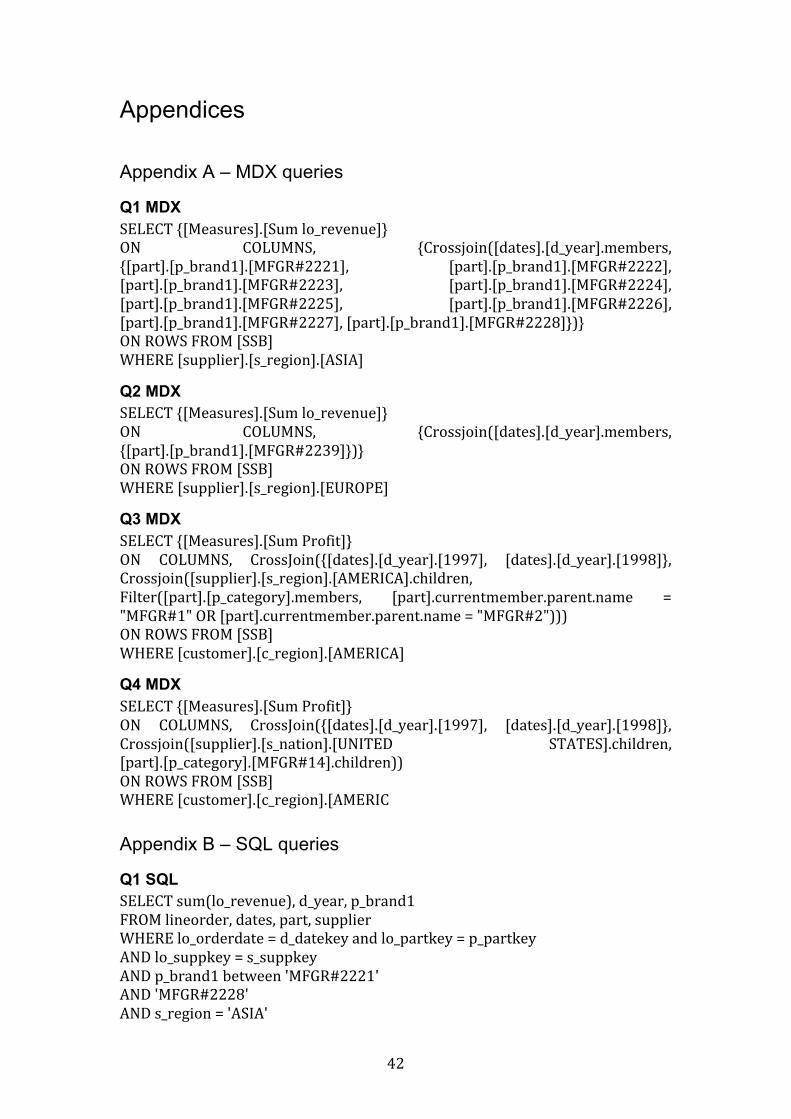
Appendix A – MDX queries

Q1 MDX SELECT{[Measures].[Sumlo_revenue]}ON COLUMNS, {Crossjoin([dates].[d_year].members,{[part].[p_brand1].[MFGR#2221], [part].[p_brand1].[MFGR#2222],[part].[p_brand1].[MFGR#2223], [part].[p_brand1].[MFGR#2224],[part].[p_brand1].[MFGR#2225], [part].[p_brand1].[MFGR#2226],[part].[p_brand1].[MFGR#2227],[part].[p_brand1].[MFGR#2228]})}ONROWSFROM[SSB]WHERE[supplier].[s_region].[ASIA]

Q2 MDX SELECT{[Measures].[Sumlo_revenue]}ON COLUMNS, {Crossjoin([dates].[d_year].members,{[part].[p_brand1].[MFGR#2239]})}ONROWSFROM[SSB]WHERE[supplier].[s_region].[EUROPE]

Q3 MDX SELECT{[Measures].[SumProfit]}ON COLUMNS, CrossJoin({[dates].[d_year].[1997], [dates].[d_year].[1998]},Crossjoin([supplier].[s_region].[AMERICA].children,Filter([part].[p_category].members, [part].currentmember.parent.name ="MFGR#1"OR[part].currentmember.parent.name="MFGR#2")))ONROWSFROM[SSB]WHERE[customer].[c_region].[AMERICA]

Q4 MDX SELECT{[Measures].[SumProfit]}ON COLUMNS, CrossJoin({[dates].[d_year].[1997], [dates].[d_year].[1998]},Crossjoin([supplier].[s_nation].[UNITED STATES].children,[part].[p_category].[MFGR#14].children))ONROWSFROM[SSB]WHERE[customer].[c_region].[AMERIC

Appendix B – SQL queries

Q1 SQL SELECTsum(lo_revenue),d_year,p_brand1FROMlineorder,dates,part,supplierWHERElo_orderdate=d_datekeyandlo_partkey=p_partkeyANDlo_suppkey=s_suppkeyANDp_brand1between'MFGR#2221'AND'MFGR#2228'ANDs_region='ASIA'

43

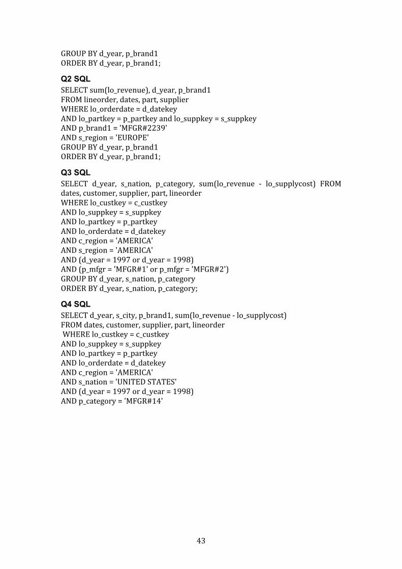
GROUPBYd_year,p_brand1ORDERBYd_year,p_brand1;

Q2 SQL SELECTsum(lo_revenue),d_year,p_brand1FROMlineorder,dates,part,supplierWHERElo_orderdate=d_datekeyANDlo_partkey=p_partkeyandlo_suppkey=s_suppkeyANDp_brand1='MFGR#2239'ANDs_region='EUROPE'GROUPBYd_year,p_brand1ORDERBYd_year,p_brand1;

Q3 SQL SELECT d_year, s_nation, p_category, sum(lo_revenue - lo_supplycost) FROMdates,customer,supplier,part,lineorderWHERElo_custkey=c_custkeyANDlo_suppkey=s_suppkeyANDlo_partkey=p_partkeyANDlo_orderdate=d_datekeyANDc_region='AMERICA'ANDs_region='AMERICA'AND(d_year=1997ord_year=1998)AND(p_mfgr='MFGR#1'orp_mfgr='MFGR#2')GROUPBYd_year,s_nation,p_categoryORDERBYd_year,s_nation,p_category;

Q4 SQL SELECTd_year,s_city,p_brand1,sum(lo_revenue-lo_supplycost)FROMdates,customer,supplier,part,lineorderWHERElo_custkey=c_custkeyANDlo_suppkey=s_suppkeyANDlo_partkey=p_partkeyANDlo_orderdate=d_datekeyANDc_region='AMERICA'ANDs_nation='UNITEDSTATES'AND(d_year=1997ord_year=1998)ANDp_category='MFGR#14'

44

Appendix C – Omicron Cluster performance Language Query 1 2 3 4 5 6 7 8 9 10MDX Q1 709 715 719 656 725 716 718 733 712 715MDX Q2 711 704 648 658 650 653 647 656 713 713MDX Q3 491 513 486 498 507 495 477 493 484 485MDX Q4 494 614 522 490 486 506 493 511 509 539SQL Q1 681 605 664 607 612 606 669 612 686 679SQL Q2 665 620 649 599 692 686 614 682 650 616SQL Q3 410 418 410 420 421 411 411 401 415 403SQL Q4 456 409 405 419 424 421 422 414 428 428

Appendix D – AWS 3 worker nodes performance

Language

Query/Attempt

1 2 3 4 5 6 7 8 9 10

MDX Q1 491 504 504 499 488 490 494 496 534 491MDX Q2 484 508 490 485 490 488 495 495 487 488MDX Q3 418 419 417 382 422 376 374 383 394 374MDX Q4 397 381 434 390 392 401 454 447 449 437SQL Q1 443 488 431 437 429 430 435 420 433 422

SQL Q2 432 434 426 435 439 437 434 436 435 427SQL Q3 361 350 343 363 361 374 369 366 364 368SQL Q4 368 366 362 354 367 356 372 348 366 368

Appendix E – AWS 6 worker nodes performance

Language

Query/Attempt

1 2 3 4 5 6 7 8 9 10

MDX Q1 298 296 290 311 293 301 307 303 297 298MDX Q2 344 299 287 306 287 295 297 305 305 325MDX Q3 256 262 234 252 261 262 261 251 270 286

MDX Q4 261 270 267 270 271 276 252 258 270 259SQL Q1 223 244 224 237 224 222 211 248 242 250SQL Q2 238 250 250 257 244 244 255 231 255 260SQL Q3 212 214 188 189 185 214 199 196 187 195SQL Q4 210 195 194 232 205 194 193 241 216 212

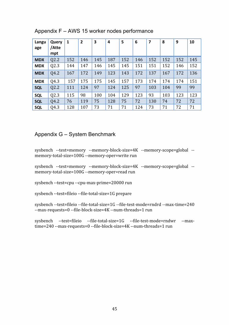
45

Appendix F – AWS 15 worker nodes performance

Language

Query/Attempt

1 2 3 4 5 6 7 8 9 10

MDX Q2.2 152 146 145 187 152 146 152 152 152 145MDX Q2.3 144 147 146 145 145 151 151 152 146 152MDX Q4.2 167 172 149 123 143 172 137 167 172 136

MDX Q4.3 157 175 175 145 157 173 174 174 174 151SQL Q2.2 111 124 97 124 125 97 103 104 99 99

SQL Q2.3 115 98 100 104 129 123 93 103 123 123SQL Q4.2 76 119 75 128 75 72 130 74 72 72SQL Q4.3 128 107 73 71 71 124 73 71 72 71

Appendix G – System Benchmark

sysbench --test=memory --memory-block-size=4K --memory-scope=global --memory-total-size=100G--memory-oper=writerunsysbench --test=memory --memory-block-size=4K --memory-scope=global --memory-total-size=100G--memory-oper=readrunsysbench--test=cpu--cpu-max-prime=20000runsysbench--test=fileio--file-total-size=1Gpreparesysbench--test=fileio--file-total-size=1G--file-test-mode=rndrd--max-time=240--max-requests=0--file-block-size=4K--num-threads=1runsysbench --test=fileio --file-total-size=1G --file-test-mode=rndwr --max-time=240--max-requests=0--file-block-size=4K--num-threads=1run