Embed Size (px)
Citation preview
UNIVERSITY OF SOUTHAMPTON
SEPTEMBER 2018
FACULTY OF NATURAL AND ENVIRONMENTAL SCIENCES
OCEAN AND EARTH SCIENCES
OPTIMISATION OF A METHOD TO QUANTIFY
MICROPLASTICS IN INTER-TIDAL SEDIMENTS
AROUND JERSEY, CHANNEL ISLANDS
by
Hannah Brittain
A dissertation submitted in partial fulfilment of the requirements for the
degree of M.Sc. Oceanography by instructional course.
DECLARATION
As the nominated University supervisor of this M.Sc. project by Hannah Brittain, I confirm
that I have had the opportunity to comment on earlier drafts of the report prior to
submission of the dissertation for consideration of the award of M.Sc. Oceanography.
Signed……………………………………………………………
Supervisor’s name:
21st September 2018
TABLE OF CONTENTS
Abstract ............................................................................................................................ I
Acknowledgements ......................................................................................................... II
List of Tables .................................................................................................................. III
List of Figures .................................................................................................................IV
1 Introduction ............................................................................................................... 1
1.1 Global Significance and Impacts of Marine Microplastic Pollution ...................... 3
1.2 Recorded Concentrations in Coastal Sediments ................................................ 4
1.3 Existing Methods to Extract Microplastics from Marine Sediments .................... 7
1.4 Research Aims and Objectives .......................................................................... 8
2 Methods .................................................................................................................... 9
2.1 Area of Study ..................................................................................................... 9
2.2 Sample Collection, Preparation and Storage ................................................... 10
2.3 Claessens et al.’s Method ................................................................................ 11
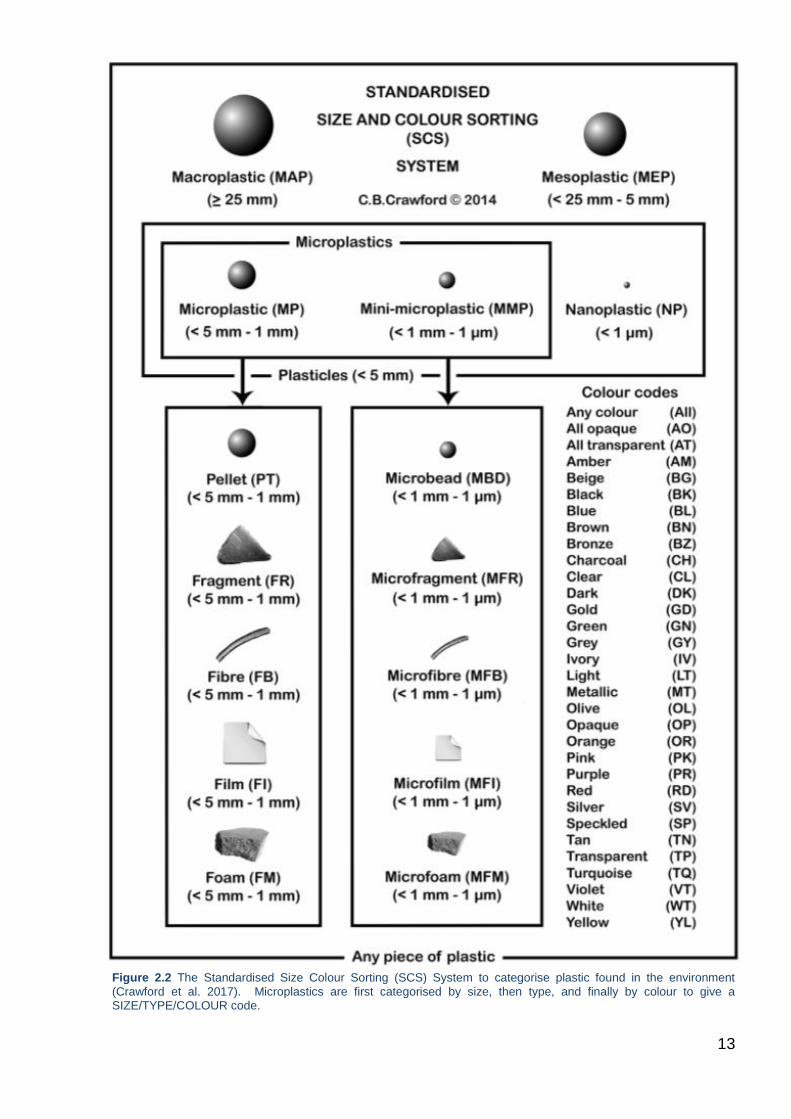
2.4 The Standardised Size Colour Sorting (SCS) System...................................... 12
2.5 Method Optimisation ........................................................................................ 14
2.5.1 Nested vs Single Sieves ............................................................................ 14
2.5.2 Considerations for microplastics < 38 μm .................................................. 14
2.5.3 Low Cost, High Density Salt Solution ........................................................ 15
2.5.4 Transferring Retained Solids to Zinc Chloride Salt Solution ...................... 15
2.5.5 Blanks Using Water of Different Origin and Purity ..................................... 16
2.6 Minimisation of Contamination ......................................................................... 17
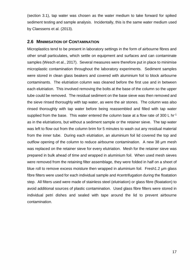
2.7 Amended Method Protocol ............................................................................... 18
2.7.1 Volume Reduction via Elutriation ............................................................... 18
2.7.2 Floatation using 7M Zinc Chloride Salt Solution ........................................ 19
2.7.3 Visual Sorting using Light Microscopy ....................................................... 19
2.8 Spiked Sediment Extraction Efficiency Tests ................................................... 20
2.9 Grain Size Analysis .......................................................................................... 20
3 Results .................................................................................................................... 21
3.1 Seawater, Tap Water and Reverse Osmosis Water Blanks ............................. 21
3.2 Spiked Sediment Extraction Efficiency Tests ................................................... 22
3.3 Jersey Intertidal Sediment Sample Analysis: Initial Observations .................... 23
3.3.1 Abundance of Material on St Aubins (SA) Filters ....................................... 23
3.3.2 Total Counts of Particles on Filters ............................................................ 24
3.4 Characteristics of Microplastics on Jersey Beaches ........................................ 25
3.4.1 Size ............................................................................................................ 25
3.4.2 Morphology ................................................................................................ 25
3.4.3 Colour ........................................................................................................ 26
3.4.4 Size and Characteristics of Large Microplastics (MP) ................................ 28
3.5 Estimates for Microplastic Contamination in the Environment .......................... 29
3.6 Grain Size Analysis and Sample Loss.............................................................. 30
4 Discussion .............................................................................................................. 32
4.1 Microplastics in Jersey Intertidal Sediments ..................................................... 32
4.2 Sources of Contamination in the Laboratory .................................................... 34
4.3 Sample Loss .................................................................................................... 36
4.4 Low Method Extraction Efficiency .................................................................... 38
4.5 Potential Impacts of Sediment Grain Size on Method Suitability ...................... 39
4.6 Identification of Microplastics using Light Microscopy ...................................... 40
5 Summary of Findings .............................................................................................. 42
6 Future Directions .................................................................................................... 43
Literature Cited .............................................................................................................. 44
Appendix .......................................................................................................................... i
COSHH and Risk Assessment Forms ........................................................................... i
Sediment Drying Regime Results .............................................................................. xiii
Catalogue Details for Microplastic Colour Examples..................................................xiv
Grain Size Analysis Data and Distribution Graphs ..................................................... xv
I
ABSTRACT
Microplastics are microscopic pieces of plastic between 1 μm – 5 mm. They are an
emerging threat to marine environments worldwide, occurring primarily through
degradation of larger items of plastic. A number of adverse effects have been
documented in marine species following exposure to microplastics, so it is important to
monitor microplastic concentrations in the marine environment to assess potential
impacts to marine ecosystems and commercial fisheries. In an attempt to address the
current lack of consensus on standardised and robust methods for microplastics
quantification, this study aimed to optimise a method to extract microplastics from
sediment samples. A method that had been proposed in the literature with promising
preliminary results was selected, then several adaptations were experimentally applied
to optimise the method. An amended method was finalised, involving three steps; 1.
Volume reduction via elutriation; 2. Extraction of microplastics via floatation and 3. Visual
sorting using a dissection microscope. The method was applied to intertidal samples
from beaches around Jersey, Channel Islands, which had not, to date, been quantified
for microplastic contamination. A microplastic profile was catalogued using visual sorting
under a dissection microscope, based on size, shape and colour of individual particles
observed. Microplastic profiles for West and East Jersey beaches were similar.
Fragments were the most common shape, and brown and black were the most common
two colours observed across both sites. However, the method had a low extraction
efficiency of 31 %, which varied across size, shape and polymer type, so the profiles
observed are not likely to be fully representative of microplastics in the environment. A
number of additional method limitations were identified, including an especially poor
extraction efficiency for microplastics > 1 mm (22 %), background contamination in the
laboratory, several potential loss steps, and the inability to confirm the synthetic polymer
origin of particles resembling microplastics. Suggested improvements were provided to
avoid similar limitations in future work. Overall these findings highlight the implicit
variance in microplastics data and substantiate the importance of clean laboratory spaces
and standardised methods for the quantification of microplastics.

II
ACKNOWLEDGEMENTS
I would like to thank my project supervisor, , for regular support and
valuable inputs on my project throughout the process. I also thank
for guiding me through the lab work and other activities during the project.
was a great help to me throughout the method optimisation phase.
assistance no doubt more than halved the time it would have taken me to carry out lab
experiments alone, and positive attitude helped me to keep striving through the
challenges this project presented.
I also thank the members of the for their thoughts and ideas
in the early stages of my project. Other notable academic contributors were
who advised me on the protocol for spiked sediment experiments; and
for their help with producing microplastics for spiked experiments;
for his help setting up the elutriation experiments in the aquarium and
lending me tools; , for allowing me use of laboratory oven to prepare
samples; for helping me with grain size analysis and for
allowing me use of the sediment dynamics lab to do so.
I extend my sincere thanks to and the team at the
and the , who
graciously collected and shipped a selection of Jersey sediment samples to upon
request.
Finally, I would like to thank my friends and coursemates, who have supported me in
countless ways towards the creation of this report.
III
LIST OF TABLES
Table 1.1 Worldwide environmental concentrations of microplastics detected in coastal sediments. Sampling continent, location, specific location, and size range, morphology and/or polymer and concentration of microplastics are listed with their corresponding studies ............................................................................................................................. 5
Table 2.1 Jersey intertidal sites sampled. Beach names are provided along with an abbreviations for the samples from each intertidal site. Exact coordinates of where the sample was collected are provided in latitude and longitude along with the date each site was sampled. ................................................................................................................ 10
Table 2.2 Polymers used in spiked sediment tests. Density and common sources from Li et al. (2016). .............................................................................................................. 20
Table 3.1 Results from the blanks, run using three water sources of different origin and purity. Three repeats were carried out with each water source; sea water, tap water and reverse osmosis (RO) water. ......................................................................................... 21
Table 3.2 Extraction efficiencies of the method using microplastics of different polymer type and size. Efficiencies were determined by running sediment spiked with 100 pieces of microplastic (one polymer type; 50 MMP, 50 MP) through one elutriation and two subsequent extractions using saturated zinc chloride salt solution. .............................. 22
Table 3.3 Profile of morphology types for microplastics > 100 μm from Jersey intertidal sediments (2 x 500 g samples). Microplastic morphology codes are from the SCS System. A count for each morphology code is listed, along with the proportion (%) that each morphology code contributes to the total microplastics count. .............................. 25
Table 3.4 Detailed catalogue of microplastics > 1 mm. Microplastics are listed under the intertidal sediment they were extracted from, with the specific sample (LB1, LB2, LE1 or LE2) and #centrifugation (C1 or C2) given in the left-hand column ............................... 28
Table 3.5 Grain size analysis results. Samples from the spiked sediment tests are prefixed with ‘S’, followed by the abbreviation for the polymer used to spike the sample. Samples from Jersey intertidal sites are prefixed with the site abbreviation, followed by the number repeat. The arithmetic (μm) and logarithmic (ϕ) mean grain size is provided for each sample, along with sand and mud content (%), overall sample loss from elutriation and sieving (%), and an overall sediment description. .................................. 30
Table 4.1 Comparison of microplastics > 1 mm observed on filters from tap water blanks and sample analyses. The total count of microplastics > 1 mm is provided along with the morphology codes for microplastics observed and the size range (measured using ImageJ). ........................................................................................................................ 34
IV
LIST OF FIGURES
Figure 1.1 Annual global plastic production from 1950 – 2015 in million metric tonnes (Mt) (Geyer et al., 2017). ................................................................................................. 1
Figure 1.2 Plastic debris nomenclature based on size, including microplastics, as proposed by the European MSFD Technical Subgroup on Marine Litter (2013). Microplastics are further split into two size categories; small microplastics (1 μm – 1 mm) and large microplastics (1 – 5 mm), to differentiate between two commonly used size ranges of microplastics in literature. Adapted from Van Cauwenberghe et al. (2015b). . 6
Figure 2.1 Map showing the study area and sample sites. (i) Jersey, Channel Islands, indicated by the red box. (ii) Intertidal sediment sampling sites for the project. The Map Key (right) indicates the method stage to which samples were analysed (1. drying -> 2. separation -> 3. microscopy). .......................................................................................... 9
Figure 2.2 The Standardised Size Colour Sorting (SCS) System to categorise plastic found in the environment (Crawford et al. 2017). Microplastics are first categorised by size, then type, and finally by colour to give a SIZE/TYPE/COLOUR code. .................. 13
Figure 2.3 Elutriation column schematic, amended from Claessens et al. (2013). ....... 18
Figure 3.1 Particulate material retained on filters from St Aubins sediment samples. Photo i) Material includes foraminifera (forams), along with some bivalve shell(s) and unidentified fibrous material. Photo ii) Light from below highlights morphological features of retained material, including forams (likely class: Miliolata; identified by their multi-chambered shells). Photo iii) Large fragment (possibly of synthetic polymer origin) covered in multiple layers of particulate biological material. Photo iv) Black plastic microfragment and microfibre intersperse biological material........................................ 23
Figure 3.2 Examples of microplastics classified as different colours under the SCS System using light microscopy. Each photograph is labelled with the colour example presented and a suitable scale ...................................................................................... 26
Figure 3.3 Percentage of different colours observed in microplastics > 100 μm extracted from Jersey intertidal sediments LB and LE. (i) Colours of 1,473 microplastics extracted from LB sediment samples (2 x 500 g). Other category includes: opaque (OP), charcoal (CH), metallic (MT) and purple (PR). (ii) Colours of 1,354 microplastics from LE sediment samples (2 x 500 g). Other category includes: olive (OL), green (GN), violet (VT), purple (PR), opaque (OP), and charcoal (CH). ........................................................................ 27
Figure 3.4 Box plots showing the estimate microplastic concentration in Jersey intertidal sediments. Units are presented as microplastics per kilogram of dry sediment (MP kg-1 DW). Calculated estimates are based on an application of standard contamination (±SD) the extraction efficiency (±SD). The red dashed line indicates the mean average, the black line in the centre of each box is the median. ........................................................ 29
Figure 4.1 Forensic approach workflows for research quantifying microplastics in environmental samples (Woodall et al. 2015)................................................................ 35
1
1 INTRODUCTION
‘Plastics’ are synthetic materials composed of many recurring smaller molecules, also
known as synthetic polymers (Crawford and Quinn, 2016). Plastics are manufactured
from organic and inorganic raw materials (i.e. carbon, silicon, hydrogen, oxygen and
chloride) which are typically extracted from oil, coal and natural gas (Shah et al., 2008).
The first modern plastic material, Bakelite (chemical name: polyoxybenzyl methylene
glycol anhydride), was developed in 1907 (Cole et al., 2011). Soon after this,
manufacturing techniques were developed through the 1940s to allow for the mass-
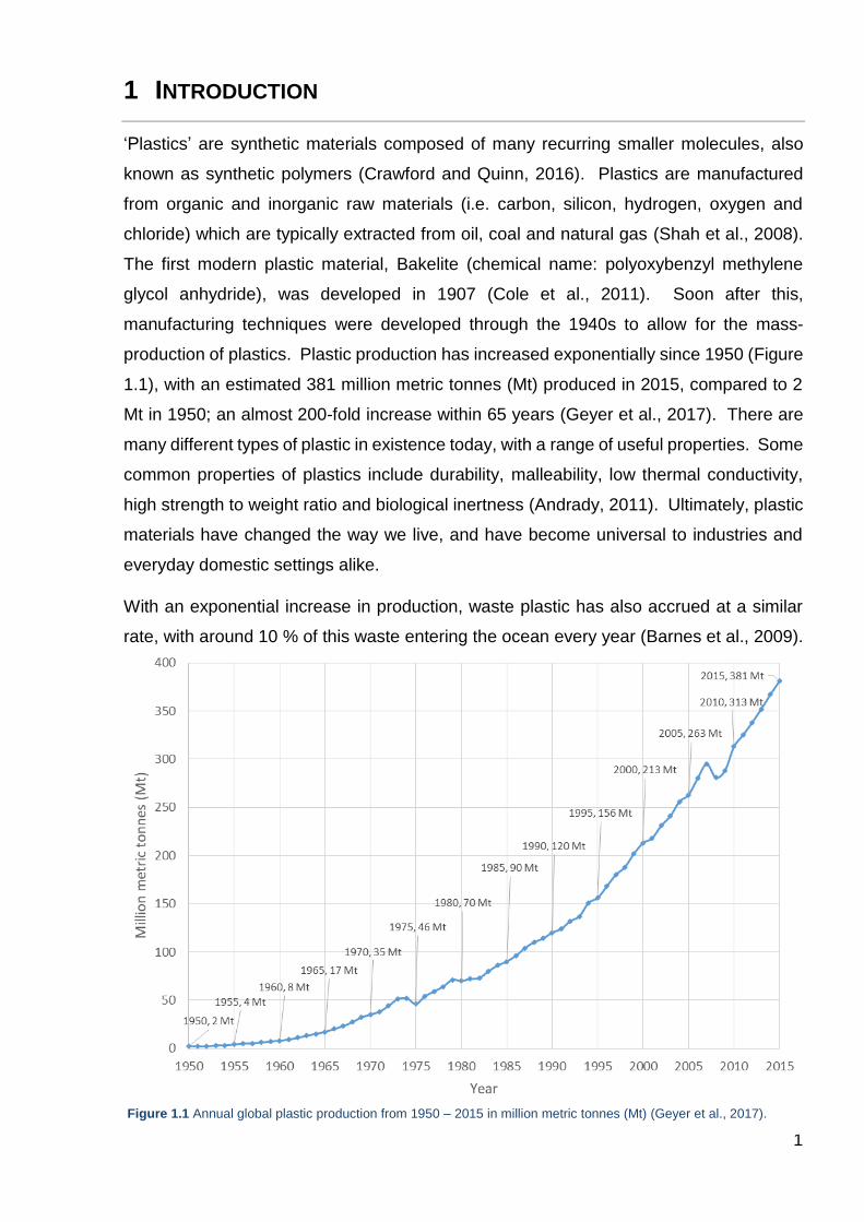
production of plastics. Plastic production has increased exponentially since 1950 (Figure
1.1), with an estimated 381 million metric tonnes (Mt) produced in 2015, compared to 2
Mt in 1950; an almost 200-fold increase within 65 years (Geyer et al., 2017). There are
many different types of plastic in existence today, with a range of useful properties. Some
common properties of plastics include durability, malleability, low thermal conductivity,
high strength to weight ratio and biological inertness (Andrady, 2011). Ultimately, plastic
materials have changed the way we live, and have become universal to industries and
everyday domestic settings alike.
With an exponential increase in production, waste plastic has also accrued at a similar
rate, with around 10 % of this waste entering the ocean every year (Barnes et al., 2009).
Figure 1.1 Annual global plastic production from 1950 – 2015 in million metric tonnes (Mt) (Geyer et al., 2017).
2
The majority of marine plastic debris originates from land-based sources (80 %), with
plastic waste being generated primarily from densely populated and industrialised areas
(Li et al., 2016). The other 20 % of plastic debris in the marine environment is ocean-
based, originating primarily from commercial fishing activities. The first reports of plastics
within marine debris date back to the 1970s (Buchanan, 1971; Carpenter and Smith Jr.,
1972; Colton et al., 1974; Gregory, 1978). These studies did not garner much attention
from the scientific community at the time. However, evidence mounted in the following
years of a variety of ecological consequences posed by plastic marine debris, such as
entanglement of large marine animals, such as turtles, in larger pieces of plastic debris
(Barnes et al., 2009; Gall and Thompson, 2015). Using worldwide data on waste and
population statistics, Jambeck et al. (2015) estimated that 4.8–12.7 million metric tonnes
of plastic waste from the land entered the marine environment in 2010 alone, with further
increases expected as plastic demand increases. The use of ‘single-use’, disposable
plastic products, such as straws and cups, has exacerbated the problem of plastic waste
by increasing the rate at which plastic becomes waste material (Ivar Do Sul and Costa,
2014).
More recently, the focus of academics has shifted towards the arguably more insidious
issue of microplastics in the marine environment (GESAMP, 2015). Microplastics are
microscopic pieces of plastic, between 1 µm – 5 mm across their widest diameter
(Germanov et al., 2018). Primary microplastics are deliberately manufactured at a
microscopic size (Boucher and Friot, 2017). This includes industrial pellets, which are
used to manufacture plastic products (Gregory, 1983), and microbeads, which have been
used widely in cosmetics products such as toothpaste and facial scrubs (Andrady, 2011).
Analysis of outfall water has indicated that microbeads from cosmetics are able to enter
the environment via wastewater treatment plants (Murphy et al., 2016). Microbeads are
currently being phased out in cosmetics in the UK following the introduction of new
legislation proposing a microbead ban in 2017 (Draft Statutory Instruments, 2017).
Secondary microplastics are more common than primary microplastics in the marine
environment, and occur as a result of degradation of larger plastic items (mesoplastics
and macroplastics) via chemical and physical processes (Sundt et al., 2014). In the
marine environment, the predominant processes, resulting in macroplastic degradation
into microplastics, include physical weathering through wave action and solar UV
photodegradation (Li et al., 2016). Secondary microplastic fibres have also been found
to leach from clothing during wash cycles, with a single garment being able to produce
>1900 fibres per wash (Browne et al., 2011).
3
1.1 GLOBAL SIGNIFICANCE AND IMPACTS OF MARINE MICROPLASTIC POLLUTION
Microplastics have been labelled as an environmental contaminant of concern, with a
number of recorded impacts on marine species (Teuten et al., 2009; Wright et al., 2013).
These impacts can be caused by microplastics as a pollutant in its own right, including
changes in behaviour, gene expression or physiological function following the ingestion
of microplastics by various marine species. For example, an exposure experiment by
Sussarellu et al. (2016) indicated that exposing the Pacific Oyster (Crassostrea gigas) to
microplastics for 2 months, at environmentally realistic concentrations, resulted in a
reduction in feeding, gamete quality and fecundity via ingestion.
There are also indirect impacts caused by microplastics in the marine environment. This
includes the ability of microplastics to absorb a range of persistent organic pollutants
(POPs) onto their surface, such as polychlorinated biphenyls (PBCs), which are toxic to
most marine organisms at high doses and associated with reduced fecundity at lower
doses (Teuten et al., 2009). For example, a study by Besseling et al. (2013) found that
weight loss and bioaccumulation of PCBs occurred in polychaetes (Arenicola marina)
following the ingestion of microplastic particles laced with PCBs. In addition, it has been
hypothesized that POPs accumulate in megafauna (i.e. mobulid rays, whale sharks and
baleen whales), through the indiscriminate filter feeding of water containing microplastics
that have absorbed POPs (Germanov et al., 2018). Environmental observations
supporting this theory include the presence of plastic additives and POPs in samples of
basking shark muscle, fin whale blubber and whale shark skin (Fossi et al., 2017, 2014,
2012). Potential impacts to megafauna include altered reproductive fitness, endocrine
disruption and general disruption to biological processes (Germanov et al., 2018).
Another impact that has been hypothesised is that biofilms which form on microplastics
could play host to harmful bacteria such as Vibrio spp. which are capable of harbouring
putative oyster pathogens (Frère et al., 2018; Harrison et al., 2014; Kirstein et al., 2016;
Zettler et al., 2013). There is also growing concern for microplastics becoming a threat
to human health, through trophic transfer of microplastics and absorbed POPs to
commercial species (Farrell and Nelson, 2013; Van Cauwenberghe and Janssen, 2014).
Considered in the light of their persistence in the marine environment, the impacts of
microplastics are a pervasive threat to all marine environments. Microplastics are
ubiquitous to marine environments globally (Eriksen et al., 2014; Germanov et al., 2018).
They have been detected throughout the water column and sediments worldwide, and
also within many marine organisms and seabirds (Andrady, 2011; Wright et al., 2013).
4
Lower density microplastics (specific gravity < 1 g cm-3), such as expanded polystyrene/
Styrofoam (EPS), tend to be positively buoyant in seawater. These microplastics can
therefore be transported thousands of miles via surface waters from their source location
due to oceanic and wind-driven currents (Baztan et al., 2014). Eriksen et al. (2014)
estimate that there are 5.25 trillion plastic particles currently floating in the oceans,
equivalent to 268,940 tonnes, with microplastics contributing 92.4 % by number of
particles and 13.2 % by weight. Subtropical gyres in particular are known to be regions
where microplastics accumulate due to oceanic currents (Cozar et al., 2014; Eriksen et
al., 2013b; Moore et al., 2001). In addition, deep sea sediments have been hypothesised
as a major sink for higher density microplastics (Van Cauwenberghe et al., 2013b;
Woodall et al., 2014). Microplastics are also prone to sinking due to biological interactions
with fouling fauna and slow sinking aggregates (Kaiser et al., 2017; Long et al., 2015). It
is hypothesized that coastal transport of microplastics, which regulates their spatial and
temporal distribution, is a major controlling process in the environmental fate and risks
posed to marine species by microplastics (Zhang, 2017).
1.2 RECORDED CONCENTRATIONS IN COASTAL SEDIMENTS
Microplastics are present in marine sediments worldwide and have been found to
accumulate in coastal regions (Zhang, 2017). A summary of recorded concentrations of
microplastics in coastal sediments is provided in Table 1.1. This covers a range of
locations around the world, but is by no means an exhaustive list. Research quantifying
microplastics in sediment has been primarily focused on intertidal and littoral zones of
beaches. Table 1.1 includes over 30 examples of beach-focused studies, spanning the
continents of Africa, America, Asia and Europe (Baztan et al., 2014; Ivar do Sul et al.,
2009; Kaberi et al., 2013; Ng and Obbard, 2006). Other coastal environments that have
been quantified for sediment microplastic concentrations include mangroves, estuaries,
harbours and subtidal bays (Claessens et al., 2011; Fok and Cheung, 2015; Mohamed
Nor and Obbard, 2014; Vianello et al., 2013).
The field of microplastics research is relatively new, with the majority of key papers
published within the last decade. As such, there has been a lack of consensus in the
literature, as the field has developed, with regards to standardised measurement units for
microplastic concentrations and the size range for microplastics (Hidalgo-Ruz et al.,
2012). This has led to a range of literature results that are difficult to compare directly
with one another , on account of the various units of measurement and size ranges
documented (Van Cauwenberghe et al., 2015b).
5
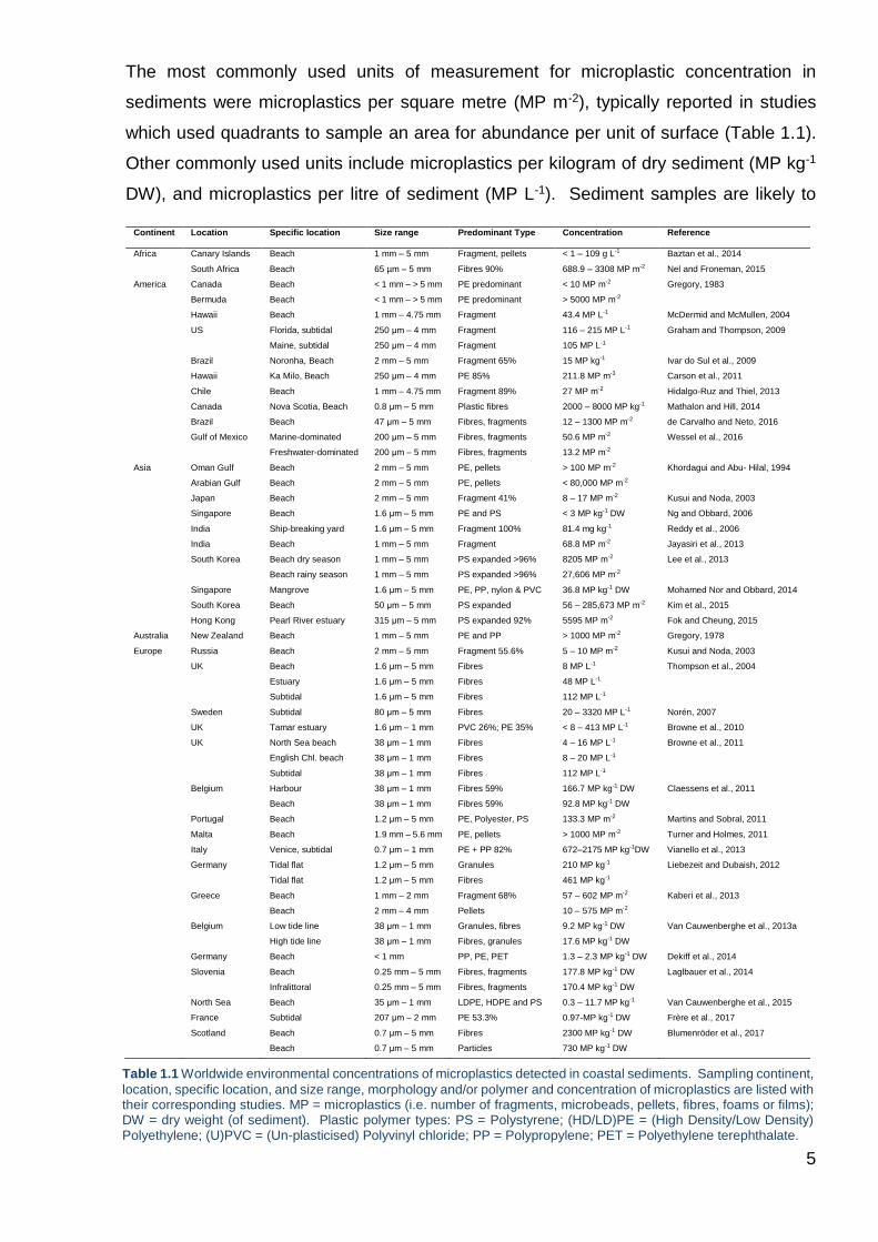
The most commonly used units of measurement for microplastic concentration in
sediments were microplastics per square metre (MP m-2), typically reported in studies
which used quadrants to sample an area for abundance per unit of surface (Table 1.1).
Other commonly used units include microplastics per kilogram of dry sediment (MP kg-1
DW), and microplastics per litre of sediment (MP L-1). Sediment samples are likely to
Table 1.1 Worldwide environmental concentrations of microplastics detected in coastal sediments. Sampling continent,
location, specific location, and size range, morphology and/or polymer and concentration of microplastics are listed with their corresponding studies. MP = microplastics (i.e. number of fragments, microbeads, pellets, fibres, foams or films); DW = dry weight (of sediment). Plastic polymer types: PS = Polystyrene; (HD/LD)PE = (High Density/Low Density) Polyethylene; (U)PVC = (Un-plasticised) Polyvinyl chloride; PP = Polypropylene; PET = Polyethylene terephthalate.
Continent Location Specific location Size range Predominant Type Concentration Reference
Africa Canary Islands Beach 1 mm – 5 mm Fragment, pellets < 1 – 109 g L-1 Baztan et al., 2014
South Africa Beach 65 µm – 5 mm Fibres 90% 688.9 – 3308 MP m-2 Nel and Froneman, 2015
America Canada Beach < 1 mm – > 5 mm PE predominant < 10 MP m-2 Gregory, 1983
Bermuda Beach < 1 mm – > 5 mm PE predominant > 5000 MP m-2
Hawaii Beach 1 mm – 4.75 mm Fragment 43.4 MP L-1 McDermid and McMullen, 2004
US Florida, subtidal 250 μm – 4 mm Fragment 116 – 215 MP L-1 Graham and Thompson, 2009
Maine, subtidal 250 μm – 4 mm Fragment 105 MP L-1
Brazil Noronha, Beach 2 mm – 5 mm Fragment 65% 15 MP kg-1 Ivar do Sul et al., 2009
Hawaii Ka Milo, Beach 250 μm – 4 mm PE 85% 211.8 MP m-3 Carson et al., 2011
Chile Beach 1 mm – 4.75 mm Fragment 89% 27 MP m-2 Hidalgo-Ruz and Thiel, 2013
Canada Nova Scotia, Beach 0.8 μm – 5 mm Plastic fibres 2000 – 8000 MP kg-1 Mathalon and Hill, 2014
Brazil Beach 47 μm – 5 mm Fibres, fragments 12 – 1300 MP m-2 de Carvalho and Neto, 2016
Gulf of Mexico Marine-dominated 200 μm – 5 mm Fibres, fragments 50.6 MP m-2 Wessel et al., 2016
Freshwater-dominated 200 μm – 5 mm Fibres, fragments 13.2 MP m-2
Asia Oman Gulf Beach 2 mm – 5 mm PE, pellets > 100 MP m-2 Khordagui and Abu- Hilal, 1994
Arabian Gulf Beach 2 mm – 5 mm PE, pellets < 80,000 MP m-2
Japan Beach 2 mm – 5 mm Fragment 41% 8 – 17 MP m-2 Kusui and Noda, 2003
Singapore Beach 1.6 μm – 5 mm PE and PS < 3 MP kg-1 DW Ng and Obbard, 2006
India Ship-breaking yard 1.6 μm – 5 mm Fragment 100% 81.4 mg kg-1 Reddy et al., 2006
India Beach 1 mm – 5 mm Fragment 68.8 MP m-2 Jayasiri et al., 2013
South Korea Beach dry season 1 mm – 5 mm PS expanded >96% 8205 MP m-2 Lee et al., 2013
Beach rainy season 1 mm – 5 mm PS expanded >96% 27,606 MP m-2
Singapore Mangrove 1.6 μm – 5 mm PE, PP, nylon & PVC 36.8 MP kg-1 DW Mohamed Nor and Obbard, 2014
South Korea Beach 50 μm – 5 mm PS expanded 56 – 285,673 MP m-2 Kim et al., 2015
Hong Kong Pearl River estuary 315 μm – 5 mm PS expanded 92% 5595 MP m-2 Fok and Cheung, 2015
Australia New Zealand Beach 1 mm – 5 mm PE and PP > 1000 MP m-2 Gregory, 1978
Europe Russia Beach 2 mm – 5 mm Fragment 55.6% 5 – 10 MP m-2 Kusui and Noda, 2003
UK Beach 1.6 μm – 5 mm Fibres 8 MP L-1 Thompson et al., 2004
Estuary 1.6 μm – 5 mm Fibres 48 MP L-1
Subtidal 1.6 μm – 5 mm Fibres 112 MP L-1
Sweden Subtidal 80 μm – 5 mm Fibres 20 – 3320 MP L-1 Norén, 2007
UK Tamar estuary 1.6 μm – 1 mm PVC 26%; PE 35% < 8 – 413 MP L-1 Browne et al., 2010
UK North Sea beach 38 μm – 1 mm Fibres 4 – 16 MP L-1 Browne et al., 2011
English Chl. beach 38 μm – 1 mm Fibres 8 – 20 MP L-1
Subtidal 38 μm – 1 mm Fibres 112 MP L-1
Belgium Harbour 38 μm – 1 mm Fibres 59% 166.7 MP kg-1 DW Claessens et al., 2011
Beach 38 μm – 1 mm Fibres 59% 92.8 MP kg-1 DW
Portugal Beach 1.2 μm – 5 mm PE, Polyester, PS 133.3 MP m-2 Martins and Sobral, 2011
Malta Beach 1.9 mm – 5.6 mm PE, pellets > 1000 MP m-2 Turner and Holmes, 2011
Italy Venice, subtidal 0.7 μm – 1 mm PE + PP 82% 672–2175 MP kg-1DW Vianello et al., 2013
Germany Tidal flat 1.2 μm – 5 mm Granules 210 MP kg-1 Liebezeit and Dubaish, 2012
Tidal flat 1.2 μm – 5 mm Fibres 461 MP kg-1
Greece Beach 1 mm – 2 mm Fragment 68% 57 – 602 MP m-2 Kaberi et al., 2013
Beach 2 mm – 4 mm Pellets 10 – 575 MP m-2
Belgium Low tide line 38 μm – 1 mm Granules, fibres 9.2 MP kg-1 DW Van Cauwenberghe et al., 2013a
High tide line 38 μm – 1 mm Fibres, granules 17.6 MP kg-1 DW
Germany Beach < 1 mm PP, PE, PET 1.3 – 2.3 MP kg-1 DW Dekiff et al., 2014
Slovenia Beach 0.25 mm – 5 mm Fibres, fragments 177.8 MP kg-1 DW Laglbauer et al., 2014
Infralittoral 0.25 mm – 5 mm Fibres, fragments 170.4 MP kg-1 DW
North Sea Beach 35 μm – 1 mm LDPE, HDPE and PS 0.3 – 11.7 MP kg-1 Van Cauwenberghe et al., 2015
France Subtidal 207 μm – 2 mm PE 53.3% 0.97-MP kg-1 DW Frère et al., 2017
Scotland Beach 0.7 μm – 5 mm Fibres 2300 MP kg-1 DW Blumenröder et al., 2017
Beach 0.7 μm – 5 mm Particles 730 MP kg-1 DW
6
contain different water content depending on temporal and spatial variables (i.e. location
on the beach, whether it was collected immediately before or after a high tide) and
sediment porosity (Van Cauwenberghe et al., 2015b). For this reason, a number of
authors have chosen to dry sediment samples before analysis, to remove water content
as a variable and allow for a more consistent comparison of data, using units of MP kg-1
DW (Claessens et al., 2011; Dekiff et al., 2014; Frère et al., 2017; Laglbauer et al., 2014;
Mohamed Nor and Obbard, 2014; Ng and Obbard, 2006; Van Cauwenberghe et al.,
2015a, 2013a; Vianello et al., 2013). This study also elected to use MP kg-1 DW for
microplastics concentration measurements.
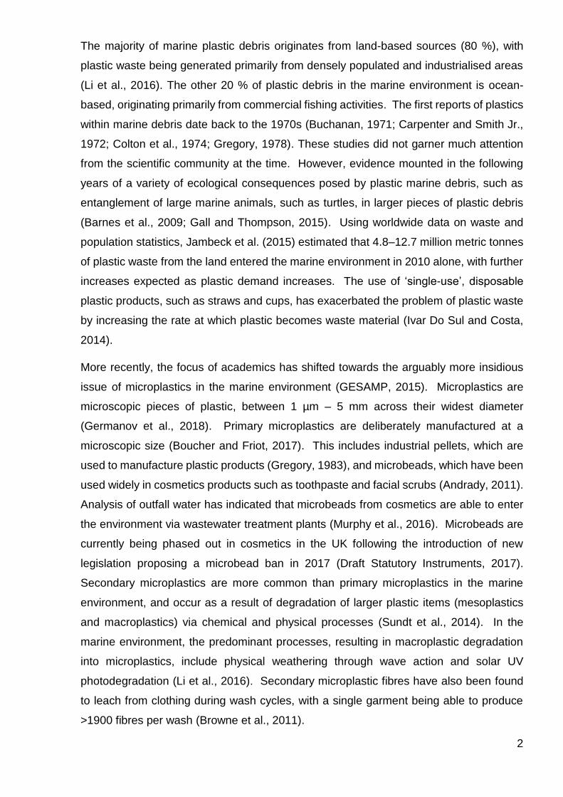
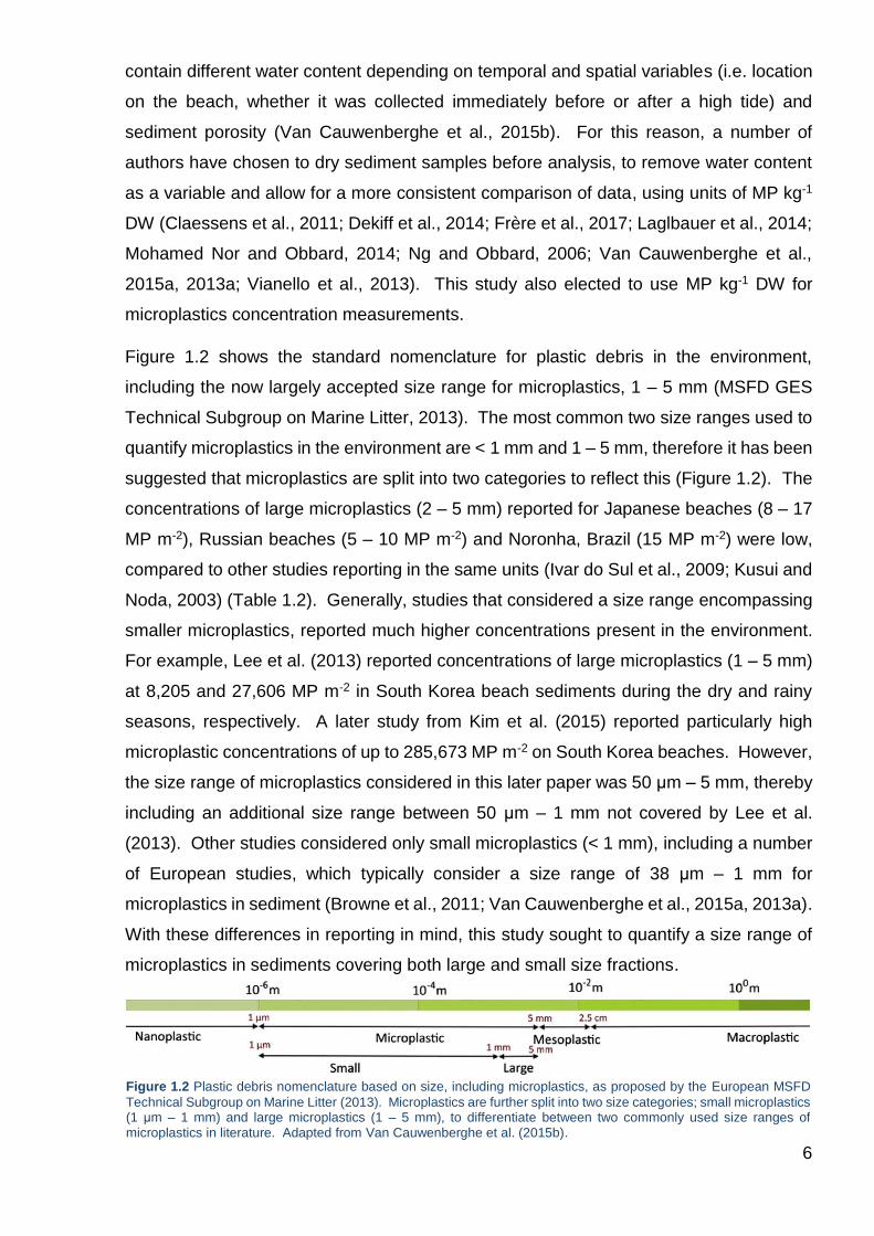
Figure 1.2 shows the standard nomenclature for plastic debris in the environment,
including the now largely accepted size range for microplastics, 1 – 5 mm (MSFD GES
Technical Subgroup on Marine Litter, 2013). The most common two size ranges used to
quantify microplastics in the environment are < 1 mm and 1 – 5 mm, therefore it has been
suggested that microplastics are split into two categories to reflect this (Figure 1.2). The
concentrations of large microplastics (2 – 5 mm) reported for Japanese beaches (8 – 17
MP m-2), Russian beaches (5 – 10 MP m-2) and Noronha, Brazil (15 MP m-2) were low,
compared to other studies reporting in the same units (Ivar do Sul et al., 2009; Kusui and
Noda, 2003) (Table 1.2). Generally, studies that considered a size range encompassing
smaller microplastics, reported much higher concentrations present in the environment.
For example, Lee et al. (2013) reported concentrations of large microplastics (1 – 5 mm)
at 8,205 and 27,606 MP m-2 in South Korea beach sediments during the dry and rainy
seasons, respectively. A later study from Kim et al. (2015) reported particularly high
microplastic concentrations of up to 285,673 MP m-2 on South Korea beaches. However,
the size range of microplastics considered in this later paper was 50 μm – 5 mm, thereby
including an additional size range between 50 μm – 1 mm not covered by Lee et al.
(2013). Other studies considered only small microplastics (< 1 mm), including a number
of European studies, which typically consider a size range of 38 μm – 1 mm for
microplastics in sediment (Browne et al., 2011; Van Cauwenberghe et al., 2015a, 2013a).
With these differences in reporting in mind, this study sought to quantify a size range of
microplastics in sediments covering both large and small size fractions.
Figure 1.2 Plastic debris nomenclature based on size, including microplastics, as proposed by the European MSFD
Technical Subgroup on Marine Litter (2013). Microplastics are further split into two size categories; small microplastics (1 μm – 1 mm) and large microplastics (1 – 5 mm), to differentiate between two commonly used size ranges of microplastics in literature. Adapted from Van Cauwenberghe et al. (2015b).
7
1.3 EXISTING METHODS TO EXTRACT MICROPLASTICS FROM MARINE SEDIMENTS
Several techniques are employed by the scientific community to extract microplastics
from sediment samples. For studies focused on intertidal areas of beaches, sediment
samples are generally collected using metal implements (i.e. iron spoon or spade) (Van
Cauwenberghe et al., 2015b). Following sample collection, a range of methods to extract
microplastics from the natural sediment matrix (typically sand) can be used. The majority
of these methods use a density separation approach, which utilises the differences in
density between plastic and natural sediment particles to isolate microplastics from
sediment. One of the simplest and most widely used methods was pioneered by
Thompson et al. (2004). This method involves agitating a sediment sample in saturated
sodium chloride (NaCl) salt solution to release microplastic particles from the sediment
matrix, which float to the surface. However, only microplastics consisting of low density
polymers (< 1.2 g cm-3) are able to be extracted using this method, as common salt
solution will not surpass a density of 1.2 g cm-3. Therefore higher density polymers will
not float to the surface and will remain in the sediment. Subsequent studies have used
different types of salt to attain a higher density salt solution and increase the extraction
efficiency for higher density polymers, such as polyvinyl chloride (PVC) (1.14 – 1.56 g
cm-3), which comprises 17 % of European plastic demand (PlasticsEurope, 2015). Zinc
chloride (ZnCl2) solution (1.5 – 1.8 g cm-3) has been used in some studies (Coppock et
al., 2017; Liebezeit and Dubaish, 2012) and sodium iodide (NaI) solution (1.3 – 1.8 g cm-
3) has been used in others (Claessens et al., 2013; Coppock et al., 2017; Dekiff et al.,
2014; Van Cauwenberghe et al., 2013a). High density microplastics are the first to sink
and intersperse with sediments (seawater density is 1.02 g cm-3), therefore it is important
that the methods used to analyse sediments are capable of extracting them (Van
Cauwenberghe et al., 2015a). One limitation in using different salt solutions is the cost
of materials. Coppock et al. (2017) provided estimate costs for NaCl, ZnCl2 and NaI
solutions of different densities. NaI and ZnCl2 solutions (1.5 g cm-3) were 41.5 and 15.6
costs units, respectively, compared to the standard cost unit for NaCl solution (1.2 g cm-
3). A new method was recently proposed by Claessens et al. (2013), which included a
prior step to reduce the overall sample size before performing a floatation with high-
density salt solution, similar to the process described above. This involved elutriation, an
upward stream of water that separates out lighter particles from denser ones. This
volume reduction step allowed for a fraction of high-density salt solution to be used per
sample, compared to the standard density separation method, which reduces the cost of
required materials significantly. In addition, the extraction efficiency of this new two-step
8
method was reported by (Claessens et al., 2013) to be more efficient than using the
flotation method alone. Claessens et al. (2013) tested the extraction efficiency of their
method by using sediments spiked with a known amount of microplastics. Retrieval rates
for microplastics were 100 % for microplastic granules, 98 % for fibres, and 100 % for
PVC fragments, compared to 75 %, 61 % and 0 %, respectively, for the standard floatation
method of Thompson et al. (2004).
1.4 RESEARCH AIMS AND OBJECTIVES
Considering the residing lack of consensus on standardised methods and reporting units
for sediment analysis, the overarching aim of this research project was to develop a
method to quantify the microplastic content of sediments. Based on the promising results
in their 2013 paper, the method proposed by Claessens et al. (2013) was used as a
starting point for method optimisation.
A need for quantification of microplastics in sediments around Jersey was highlighted in
a project proposal from the States of Jersey’s Department of the Environment (DoE).
Contact was made with the DoE, who collaborated on this research project in order that
the optimised method could be applied to Jersey intertidal sediment samples to assess
microplastic contamination around the island.
Objectives:
1. Optimise a method to analyse sediment samples for microplastic content, based
on the method put forward by Claessens et al. (2013).
2. Achieve a consistent method efficiency (microplastic recovery rate) of > 90 %
3. Apply the optimum method to intertidal sediment samples from Jersey and quantify
microplastic contamination.
4. Create a microplastic profile for Jersey beaches (i.e. size, morphology and colour
of microplastics).
9
2 METHODS
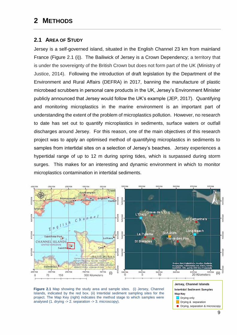
2.1 AREA OF STUDY
Jersey is a self-governed island, situated in the English Channel 23 km from mainland
France (Figure 2.1 (i)). The Bailiwick of Jersey is a Crown Dependency; a territory that
is under the sovereignty of the British Crown but does not form part of the UK (Ministry of
Justice, 2014). Following the introduction of draft legislation by the Department of the
Environment and Rural Affairs (DEFRA) in 2017, banning the manufacture of plastic
microbead scrubbers in personal care products in the UK, Jersey’s Environment Minister
publicly announced that Jersey would follow the UK’s example (JEP, 2017). Quantifying
and monitoring microplastics in the marine environment is an important part of
understanding the extent of the problem of microplastics pollution. However, no research
to date has set out to quantify microplastics in sediments, surface waters or outfall
discharges around Jersey. For this reason, one of the main objectives of this research
project was to apply an optimised method of quantifying microplastics in sediments to
samples from intertidal sites on a selection of Jersey’s beaches. Jersey experiences a
hypertidal range of up to 12 m during spring tides, which is surpassed during storm
surges. This makes for an interesting and dynamic environment in which to monitor
microplastics contamination in intertidal sediments.
Figure 2.1 Map showing the study area and sample sites. (i) Jersey, Channel
Islands, indicated by the red box. (ii) Intertidal sediment sampling sites for the project. The Map Key (right) indicates the method stage to which samples were
analysed (1. drying -> 2. separation -> 3. microscopy).
(ii) (i)
Drying, separation & microscopy
Drying & separation
Drying only
10
2.2 SAMPLE COLLECTION, PREPARATION AND STORAGE
The States of Jersey Department of the Environment (DoE) collaborated on this research
project and, as part of this collaborative effort, very kindly collected and shipped a number
of sediment samples to the National Oceanography Centre upon request. Figure 2.1 (ii)
indicates the sample collection sites on a map of Jersey, and Table 2.1 provides the exact
coordinates and a description of each of the intertidal sites selected by the author.
These sites were chosen to provide a spatial range across the island with varied levels of
anthropogenic impact in different sites i.e. some sites are close to outfall sources, which
are well-documented as sources of microplastics to the environment in the literature
(Browne et al., 2011; Lourenço et al., 2017; Stolte et al., 2015). Samples were collected
by the States of Jersey DoE on 29 – 30 May 2018. A total of 4 x 500 g samples were
collected for each site, along a 4 m transect parallel to the tide line. Each sample was
collected approximately 1 m apart to 100 mm depth.
Samples were then shipped to the National Oceanography Centre Southampton in
separate sealed polyethylene bags. Upon arrival in the laboratory, sediment samples
were transferred to glass beakers which had been cleaned previously in an acid wash
(Hydrochloric acid; HCl) and covered in aluminium foil to minimise airbourne
contamination. All samples were prepared for analysis by drying in an oven or autoclave
to remove excess water content. Full drying regime details in the Appendix (Table i).
Due to time constraints imposed by an extended period of method optimisation, three
sites of the eight sampled were prioritised for further analysis; Long Beach (LB), L’Etacq
(LE) and St Aubins (SA). These sites were prioritised because they offered a broad
spread of locations around the island. This included one western, storm-washed site,
one southern site in close proximity to an outfall source, and one eastern beach within a
RAMSAR site. Following the extraction of microplastics from sediment, each remaining
sediment sample was recovered and transferred to a glass beaker. During grain size
analysis, sediments were stored in disposable aluminium trays with paper lids.
Beach name Abbrev. Latitude Longitude Date collected Description of intertidal site
Long Beach LB 49.195 -2.030 29/05/2018 East, RAMSAR site
L’Etacq LE 49.240 -2.245 30/05/2018 West, storm washed
St Aubins SA 49.191 -2.131 30/05/2018 South, near outfall source
Harve des Pas HP 49.177 -2.100 29/05/2018 South beach
St Catherine’s SC 49.228 -2.024 29/05/2018 North East sheltered bay
Greve de L’Ecq GE 49.247 -2.202 30/05/2018 North bay
La Pulante LP 49.190 -2.230 30/05/2018 West, near outfall
St Brelades SB 49.185 -2.198 30/05/2018 South West bay
Table 2.1 Jersey intertidal sites sampled. Beach names are provided along with an abbreviations for the samples from
each intertidal site. Exact coordinates of where the sample was collected are provided in latitude and longitude along with the date each site was sampled.
11
2.3 CLAESSENS ET AL.’S METHOD
The method in this study was optimised from a method presented by Claessens et al.
(2013), described below.
Claessens et al. (2013) developed a device to carry out elutriation on sediment samples,
using an upward flow of water to separate lighter particles in the sediment matrix,
including microplastics, from denser ones. The aim of elutriation was to achieve a sample
volume reduction before undergoing floatation in high density salt solution. The device
used was a PVC column, with tap water entering from the base and an aeration stone
arrangement at the bottom of the column to ensure efficient separation of sediment
particles. Sediment samples were washed through a 1 mm sieve into the column, then
tap water was forced in through the base. It was experimentally determined that the flow
rate for tap water should be set at 300 L hr-1 and run for 15 minutes. This rate was found
to be adequate to keep sand particles in the tube whilst other material, including
microplastics, flowed over the edge. Lighter particulates were transported to the top of
the column with the rising water, and eventually flowed out with the supernatant water.
Solids were retained on a 35 μm sieve.
The second step following volume reduction through elutriation, was floatation. Solids
retained on the 35 μm sieve were transferred to a 50 mL centrifuge tube and 40 mL of
high density NaI solution (1.6 g cm-3) was added. This was followed by vigorous manual
shaking and centrifugation for 5 minutes at 3,500 g. The top layer of salt solution
containing microplastics was then vacuum filtered over 5 μm sieve. This floatation step
was repeated 2 – 3 times to ensure all microplastics were extracted from the sample.
Visual inspection of the filter was carried out using a dissection microscope.
Claessens et al. (2013) also carried out a method validation phase to determine the
extraction efficiency of their newly developed method and compare with the method
pioneered. This phase involved evaluating both techniques using sediments spiked with
a known concentration of fibres or granules before subjecting these sediments to either
one of the techniques. Clean sediment was obtained by subjecting sediment to several
elutriations to remove all microplastics present in the sediment matrix. The microplastics
used to spike the clean sediment samples were polyvinyl chloride (PVC) granules,
polyethylene (PE) granules and fibres (polymer(s) unknown) that had been previously
extracted from environmental sediment samples. 50 particles or fibres were used to spike
each sediment sample. As mentioned previously, the results of this method validation
indicated that retrieval rates for microplastics were 100 % for microplastic granules, 98 %
12
for fibres, and 100 % for PVC fragments, compared to 75 %, 61 % and 0 %, respectively,
for the standard floatation method of Thompson et al. (2004).
2.4 THE STANDARDISED SIZE COLOUR SORTING (SCS) SYSTEM
The Standardised Size Colour Sorting (SCS) System (Crawford et al., 2017) was used to
categorise all microplastics based on their size and appearance (Figure 2.2). The SCS
System is able to categorise any plastic, but for the purposes of this study, only the
microplastics size range (1 μm – 5 mm) was utilised.
Step 1: Category (size)
The first step in using the SCS System was to sort plastics into categories, based on their
size. Size was measured as the entire length for fibres, and the widest diameter for other
microplastics. The microplastics (MP) category covers all plastics between < 5 mm – 1
mm, and the mini-microplastic (MMP) category covers all plastics between < 1 mm – 1
μm, along their longest dimension. All MP category microplastics were measured using
ImageJ.
Step 2: Type
Microplastics were then categorised based on their morphology, with five subcategories
under each size category (MP and MMP). Under the MP category, spherical pieces of
plastic were labelled ‘Pellet’ (PT), irregular shaped pieces of plastic were labelled
‘Fragment’ (FR), strands or filaments of plastic were labelled ‘Fibre’ (FB), thin sheets or
membrane-like pieces of plastic were labelled ‘Film’ (FI), and pieces of sponge, foam, or
foam-like plastic material were labelled ‘Foam’ (FM). Under the MMP category, spherical
pieces of plastic were labelled ‘Microbead’ (PT), irregular shaped pieces of plastic were
labelled ‘Microfragment’ (FR), strands or filaments of plastic were labelled ‘Microfibre’
(FB), thin sheets or membrane-like pieces of plastic were labelled ‘Microfilm’ (FI), and
pieces of sponge, foam, or foam-like plastic material were labelled ‘Microfoam’ (FM).
Step 3: Colour
Next, microplastics were all given an individual colour code from the listed codes in the
right-hand panel on Figure 2.2.
Example: An irregularly shaped piece of plastic, 0.8 mm in length across the widest
diameter, which is green in colour would be given the label ‘MMP/MFR/GN’ according to
the SCS System.
13
Figure 2.2 The Standardised Size Colour Sorting (SCS) System to categorise plastic found in the environment
(Crawford et al. 2017). Microplastics are first categorised by size, then type, and finally by colour to give a SIZE/TYPE/COLOUR code.
14
2.5 METHOD OPTIMISATION
A major portion of this research project was devoted to method optimisation. This was
conducted by testing a range of adaptations to try and improve different aspects of the
method put forward by Claessens et al. (2013).
2.5.1 Nested vs Single Sieves
In order to cover the full range of microplastics, it was decided that the method should be
amended to extract microplastics up to 5 mm. Claessens et al. (2013) sieved their
sediment samples down to 1 mm before elutriation, therefore only microplastics < 1 mm
were considered. The use of nested sieve filters, at 1 mm and 38 μm apertures, was
tested for the elutriation step to keep these larger and smaller size fractions of
microplastics separate from the outset. The outcome of these tests indicated that nothing
was gained from adding an additional mesh to the sieve (1 mm), as very little material
was retained > 1 mm, and the size of larger particulates could be confirmed using visual
microscopy with the use of a single sieve to retain material following elutriation. Therefore
a single sieve at 38 μm was used, as in Claessens et al. (2013).
2.5.2 Considerations for microplastics < 38 μm
A protocol to recover microplastics < 38 μm was researched, and tested, where possible.
It was hoped that an additional size range of 1.2 – 38 μm could be quantified using an
amended method. This size range of microplastics is the most likely to impact on benthic
species important to Jersey’s commercial fisheries, such as the Pacific Oyster
(Crassostrea gigas) and the King scallop (Pecten maximus). This is due to their similar
size to filter-fed particulate matter, making these smaller microplastics more likely to be
ingested by these species via filtration (Brillant and MacDonald, 2000; Sussarellu et al.,
2016; Van Cauwenberghe and Janssen, 2014).
I. Smaller Mesh for Elutriation
Due to the flow rate of the elutriation (300 L hr-1), it was not possible to simply add or
replace the existing 38 μm mesh with a smaller mesh. This is because the flow rate
would be likely to exceed the filtration rate at such a small aperture (1.2 μm), and more
markedly so with the accumulation of material on the filter throughout the process of
elutriation. This would therefore greatly increase a risk of overspill, resulting in sample
loss. Other protocols to tackle this size range were therefore considered.
15
II. Vacuum Filtration of Collected Water
One protocol was tested, which involved vacuum filtration of the water that had been
through an elutriation step. A 200 L glass tank was cleaned (rinsed thoroughly with
tap water) and used to collect the 75 L of water which had been through elutriation.
Foil was used to cover the tank to reduce airbourne contamination. This water was
then vacuum filtered onto several 1.2 μm glass fibre filters to retain particulates
(including microplastics) between 1.2 – 38 μm. This additional step added
approximately 15 hours to a 1 hour protocol, per sample. Furthermore, this method
was subject to additional contamination on account of the length of time taken to
complete the filtration, which allowed for dust to settle out and contaminate the water
in the tank overnight. This protocol was therefore discarded, on account of its time-
consuming nature and unreliability of the data collected due to contamination.
III. Tangential Flow Filtration
Another protocol was considered, but was not possible to test within the scope of this
project. This proposed the use of a Tangential Flow Filtration (TFF) system, which
has been used in previous studies to separate microbes and viruses from marine
water samples (Cai et al., 2015). It was suggested that this principle could be used to
separate microplastics from water samples, specifically from the water which had
undergone elutriation. Unfortunately it was not possible to source a TFF System
within the scope of this project.
The results of this research indicated that the options for processing microplastics < 38
μm were limited, and difficult to apply to Claessens et al.'s method (2013). Therefore it
was decided that only microplastics > 38 μm would be considered.
2.5.3 Low Cost, High Density Salt Solution
The approximate costs to make salt solution with 1.5 g cm-3 density are £35.10 L-1 for
ZnCl2 and £172.95 L-1 for NaI (Coppock et al., 2017). Due to the considerable difference
in material costs, yet relatively similar density that could be achieved, ZnCl2 solution (1.5
g cm-3) was chosen as the floatation medium, in substitution of NaI solution (1.6 g cm-3),
which was used by Claessens et al. (2013).
2.5.4 Transferring Retained Solids to Zinc Chloride Salt Solution
Claessens et al. (2013) state that the step following each elutriation is to transfer the
solids to a 50 mL centrifuge tube for the floatation step. However, it is not explicitly
detailed in the paper how to do so. Therefore several different protocols were considered.
16
I. Scrape Material off Filter
Firstly, the use of a metal implement to scrape material from the filter to the centrifuge
tube was considered. This protocol, or similar, was assumed to be the method used
by Claessens et al. (2013), despite the ambiguity of the transfer method detailed in
the paper, hence was the first to be considered. As this method would rely on visual
inspection of the filter to ensure all material was transferred, it was deemed to add an
unnecessary potential loss step for smaller microplastics, which are difficult to see
with the naked eye and thus ensure their transfer to the tube. Therefore other
protocols were considered which involved transferring the filter to the tube along with
any retained solids.
II. Add Whole Filter to Tube
A second consideration was to transfer the filter as a whole to the tube. However, as
the circular filter had 15 cm diameter, it needed to be folded before adding it to the
tube. This meant that it was difficult to achieve a transfer without trapping retained
material (including microplastics) within the folds of the filter, thus reducing the
extraction efficiency of the floatation step. This protocol was therefore deemed
impractical.
III. Cut Up and Add Filter to Tube
In this protocol, filters were cut up before floatation was performed. Firstly, any visible
material retained on the filter was scraped into the tube using a clean metal spatula.
Then the filters were cut into approx. 0.5 – 1 mm pieces in a clean glass container
being added to the centrifuge tube. This aimed to reduce the potential for
microplastics being trapped during floatation whilst ensuring that the majority of
retained material was transferred to the centrifuge tube.
Protocol III. was used for all subsequent ZnCl2 floatation steps for sample analysis.
2.5.5 Blanks Using Water of Different Origin and Purity
Blanks were carried out using different water mediums, to determine which would be the
most suitable for the method by minimising contamination. The water mediums tested
were of different origins and purity, and included sea water (filtered through sand to
remove large particulates), tap water and reverse osmosis (RO) water. Three blanks
were carried out, for each water medium, through the full method protocol (without a
sediment sample). Microplastic contamination on the filters following the blanks being
carried out was categorised using the SCS System. Based on the results of these tests
17
(section 3.1), tap water was chosen as the water medium to take forward for spiked
sediment testing and sample analysis. Incidentally, this is the same water medium used
by Claessens et al. (2013).
2.6 MINIMISATION OF CONTAMINATION
Microplastics tend to be present in laboratory settings in the form of airbourne fibres and
other small particulates, which settle on equipment and surfaces and can contaminate
samples (Wesch et al., 2017). Several measures were therefore put in place to minimise
microplastic contamination throughout the laboratory experiments. Sediment samples
were stored in clean glass beakers and covered with aluminium foil to block airbourne
contaminants. The elutriation column was cleaned before the first use and in between
each elutriation. This involved removing the bolts at the base of the column so the upper
tube could be removed. The residual sediment on the base sieve was then removed and
the sieve rinsed thoroughly with tap water, as were the air stones. The column was also
rinsed thoroughly with tap water before being reassembled and filled with tap water
supplied from the base. This water entered the column base at a flow rate of 300 L hr-1
as in the elutriations, but without a sediment sample or the retainer sieve. The tap water
was left to flow out from the column brim for 5 minutes to wash out any residual material
from the inner tube. During each elutriation, an aluminium foil lid covered the top and
outflow opening of the column to reduce airbourne contamination. A new 38 μm mesh
was replaced on the retainer sieve for every elutriation. Mesh for the retainer sieve was
prepared in bulk ahead of time and wrapped in aluminium foil. When used mesh sieves
were removed from the retaining filter assemblage, they were folded in half on a sheet of
blue roll to remove excess moisture then wrapped in aluminium foil. Fresh1.2 μm glass
fibre filters were used for each individual sample and #centrifugation during the floatation
step. All filters used were made of stainless steel (elutriation) or glass fibre (floatation) to
avoid additional sources of plastic contamination. Used glass fibre filters were stored in
individual petri dishes and sealed with tape around the lid to prevent airbourne
contamination.
18
2.7 AMENDED METHOD PROTOCOL
Following the method optimisation phase, an amended method protocol was established
for the extraction of microplastics from sediment samples.
2.7.1 Volume Reduction via Elutriation
A custom-made PVC column was made to the specification of Claessens et al. (2013) to
carry out elutriation on sediment samples (Figure 2.3). The column and airstones were
cleaned with tap water prior to use. A 500 g dry sediment sample was washed through
a 5 mm mesh into a 2 L beaker to remove
larger particles from the sediment, then
carefully washed into the elutriation
column from the top. Airstones were then
turned on and placed into the column from
the top, and the column openings were
covered with aluminium foil (without
blocking the supernatant outflow) to
reduce airbourne contamination. Tap
water flow rate was measured to 300 L hr-
1 using a measuring flask and timer (12
second to fill up to the 1 L mark). The tap
water was then supplied to the column via
a pipe attached to the base. Elutriation
was carried out for 15 minutes from the
time the supernatant water started to exit
the overflow, with lighter solids (including
microplastics) being retained on the 38
μm (retainer sieve). During elutriation, the
filter was monitored to ensure retained
material did not block the flow of water and cause an overflow. At the end of the 15
minute elutriation, the tap water supply was removed from the base of the column and
water allowed to flow out. Remaining sediment was retained on the base sieve, and was
retrieved by removing the column from the base. Lighter solids that were retained on the
retainer sieve were removed with the mesh from the retainer sieve holder. The mesh was
carefully folded in half to keep solids from being inadvertently lost, then placed on a piece
of blue roll to remove excess moisture and wrapped in aluminium foil.
Figure 2.3 Elutriation column schematic, amended from Claessens et al. (2013).
retainer sieve
base sieve
19
2.7.2 Floatation using 7M Zinc Chloride Salt Solution
Following volume reduction of a sample through elutriation, microplastics were extracted
from the material retained on the 38 μm sieve using 7M zinc chloride solution (ZnCl2) (1.5
g cm-3).
Preparation of ZnCl2 solution was carried out in a fume cupboard and was made to the
specifications of (Coppock et al., 2017). 1 L of Milli-Q ultrapure water was added to a 5
L conical flask. Following this, ZnCl2 powder (Arcos Organics Zinc Chloride 98+% extra
pure) was weighed out to 972 g in a fume cupboard, then added to the Milli-Q water. This
was then manually stirred for approximately 5 minutes (or until all solids had visibly
dissolved). The process of dissolving the salt powder in water resulted in an exothermic
reaction, thus the solution was left in the fume cupboard for 60 minutes to cool. The ZnCl2
solution was then vacuum filtered using 1.2 μm glass fibre filters to remove any
undissolved salt crystals. Prepared ZnCl2 was stored in 50 mL centrifuge tubes in batches
of 40 mL, ready for floatation.
The solids and 38 μm sieve filter were then transferred to a 50 mL centrifuge tube filled
with 40 mL 7M ZnCl2 solution using the method described in section 2.5.4 (III. Cut Up and
Add Filter to Tube). This was followed by vigorous manual shaking and centrifugation for
5 minutes at 3,500 g (Hettich Zentrifugen Rotana 460R. Settings: 18°C; 3,500 g; 05:00).
The top layer of salt solution (containing microplastics) was then vacuum filtered over 1.2
μm sieve using glass pipettes that been altered so that the wider aperture end could be
used to collect larger material floating in the salt solution. This floatation step was
repeated 2 times to ensure all microplastics were extracted from the sample.
2.7.3 Visual Sorting using Light Microscopy
Visual inspection of the filter was carried out using a dissection light microscope (Olympus
BH-2) and a photographic catalogue was kept of each section of the filter where
microplastics were present using a Nikon D5000 camera. Microplastics were sorted
according to the SCS System (section 2.4) (Crawford et al., 2017). Details of the
microplastics observed were catalogued in an Excel spreadsheet for each sample, which
included the date, photo number, sample (site and #repeat), #centrifugation, size
(MP/MMP), type (morphology), colour, count (# microplastics of the same SCS code),
and exact size for microplastics > 1 mm (MP only).
20
2.8 SPIKED SEDIMENT EXTRACTION EFFICIENCY TESTS
Bulk sediment for the spiked sediment tests was collected at Hayling Island,
(50°47'37.5"N, 1°01'29.9"W). Prior to being spiked, sediment was put through several
elutriations to remove any microplastics present, before being dried at 60 °C for 24 hrs.
Clean dry sediment was then weighed out to 500 g samples and stored in glass beakers
covered in aluminium foil, ready to be spiked with a known amount of microplastics.
Three polymer types were used for the spiked sediment tests; nylon/ polyamide (PA),
polystyrene (PS) and polyvinyl chloride (PVC) (Table 2.2). These polymer types were
used as they are commonly found in marine sediments (Table 1.1). PS and PVC
microplastics were created using a band saw to cut fragments and microfragments from
larger plastic items (PS coffee cup lid/ tray and PVC column offcut). PA microplastics
were created by distressing tulle fabric to create fibres and microfibres. Microplastics
were sorted into MP and MMP size fractions by sieving through a 1 mm mesh, then
collecting the different size fraction in glass vials. Three sediment samples were used for
the spiked sediment tests, with a different polymer in each sample. Each sediment
sample was spiked with 50 x MP and 50 x MMP of a polymer type, to a total of 100
microplastics, which were counted out with the aid of a dissection microscope and fine
tweezers. Spiked sediments were then put through the full amended method to determine
the extraction efficiency by the amount of microplastics extracted.
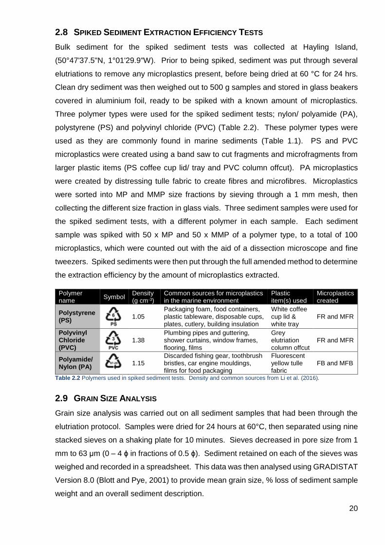
Table 2.2 Polymers used in spiked sediment tests. Density and common sources from Li et al. (2016).
2.9 GRAIN SIZE ANALYSIS
Grain size analysis was carried out on all sediment samples that had been through the
elutriation protocol. Samples were dried for 24 hours at 60°C, then separated using nine
stacked sieves on a shaking plate for 10 minutes. Sieves decreased in pore size from 1
mm to 63 μm (0 – 4 ϕ in fractions of 0.5 ϕ). Sediment retained on each of the sieves was
weighed and recorded in a spreadsheet. This data was then analysed using GRADISTAT
Version 8.0 (Blott and Pye, 2001) to provide mean grain size, % loss of sediment sample
weight and an overall sediment description.
Polymer name
Symbol Density (g cm-3)
Common sources for microplastics in the marine environment
Plastic item(s) used
Microplastics created
Polystyrene (PS)
1.05
Packaging foam, food containers, plastic tableware, disposable cups, plates, cutlery, building insulation
White coffee cup lid & white tray
FR and MFR
Polyvinyl Chloride (PVC)
1.38 Plumbing pipes and guttering, shower curtains, window frames, flooring, films
Grey elutriation column offcut
FR and MFR
Polyamide/ Nylon (PA)
1.15
Discarded fishing gear, toothbrush bristles, car engine mouldings, films for food packaging
Fluorescent yellow tulle fabric
FB and MFB
21
3 RESULTS
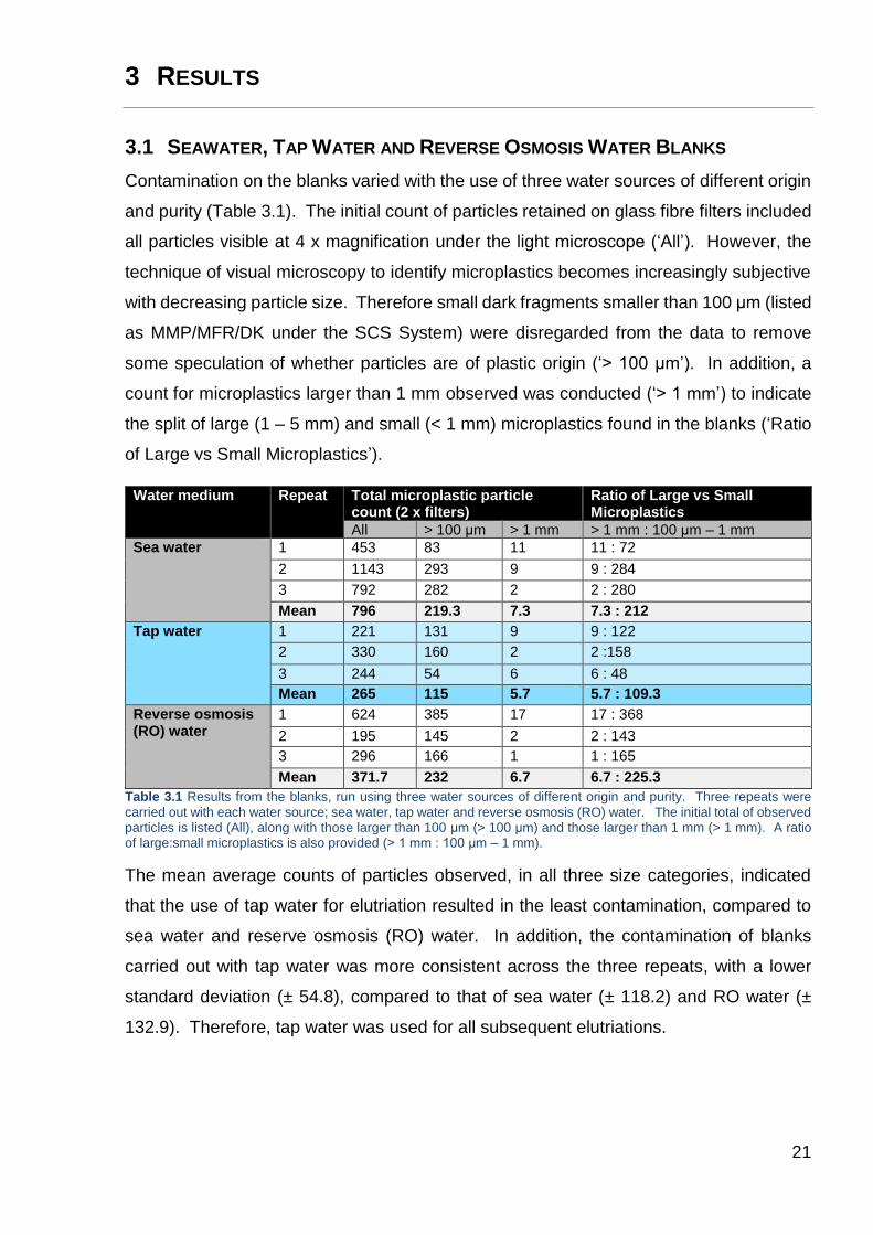
3.1 SEAWATER, TAP WATER AND REVERSE OSMOSIS WATER BLANKS
Contamination on the blanks varied with the use of three water sources of different origin
and purity (Table 3.1). The initial count of particles retained on glass fibre filters included
all particles visible at 4 x magnification under the light microscope (‘All’). However, the
technique of visual microscopy to identify microplastics becomes increasingly subjective
with decreasing particle size. Therefore small dark fragments smaller than 100 μm (listed
as MMP/MFR/DK under the SCS System) were disregarded from the data to remove
some speculation of whether particles are of plastic origin (‘> 100 μm’). In addition, a
count for microplastics larger than 1 mm observed was conducted (‘> 1 mm’) to indicate
the split of large (1 – 5 mm) and small (< 1 mm) microplastics found in the blanks (‘Ratio
of Large vs Small Microplastics’).
Water medium Repeat Total microplastic particle count (2 x filters)
Ratio of Large vs Small Microplastics
All > 100 μm > 1 mm > 1 mm : 100 μm – 1 mm
Sea water 1 453 83 11 11 : 72
2 1143 293 9 9 : 284
3 792 282 2 2 : 280
Mean 796 219.3 7.3 7.3 : 212
Tap water 1 221 131 9 9 : 122
2 330 160 2 2 :158
3 244 54 6 6 : 48
Mean 265 115 5.7 5.7 : 109.3
Reverse osmosis (RO) water
1 624 385 17 17 : 368
2 195 145 2 2 : 143
3 296 166 1 1 : 165
Mean 371.7 232 6.7 6.7 : 225.3
Table 3.1 Results from the blanks, run using three water sources of different origin and purity. Three repeats were
carried out with each water source; sea water, tap water and reverse osmosis (RO) water. The initial total of observed particles is listed (All), along with those larger than 100 μm (> 100 μm) and those larger than 1 mm (> 1 mm). A ratio of large:small microplastics is also provided (> 1 mm : 100 μm – 1 mm).
The mean average counts of particles observed, in all three size categories, indicated
that the use of tap water for elutriation resulted in the least contamination, compared to
sea water and reserve osmosis (RO) water. In addition, the contamination of blanks
carried out with tap water was more consistent across the three repeats, with a lower
standard deviation (± 54.8), compared to that of sea water (± 118.2) and RO water (±
132.9). Therefore, tap water was used for all subsequent elutriations.
22
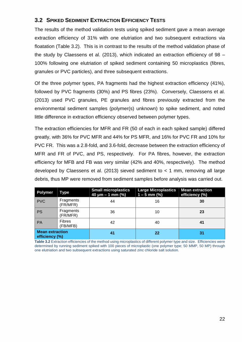
3.2 SPIKED SEDIMENT EXTRACTION EFFICIENCY TESTS
The results of the method validation tests using spiked sediment gave a mean average
extraction efficiency of 31% with one elutriation and two subsequent extractions via
floatation (Table 3.2). This is in contrast to the results of the method validation phase of
the study by Claessens et al. (2013), which indicated an extraction efficiency of 98 –
100% following one elutriation of spiked sediment containing 50 microplastics (fibres,
granules or PVC particles), and three subsequent extractions.
Of the three polymer types, PA fragments had the highest extraction efficiency (41%),
followed by PVC fragments (30%) and PS fibres (23%). Conversely, Claessens et al.
(2013) used PVC granules, PE granules and fibres previously extracted from the
environmental sediment samples (polymer(s) unknown) to spike sediment, and noted
little difference in extraction efficiency observed between polymer types.
The extraction efficiencies for MFR and FR (50 of each in each spiked sample) differed
greatly, with 36% for PVC MFR and 44% for PS MFR, and 16% for PVC FR and 10% for
PVC FR. This was a 2.8-fold, and 3.6-fold, decrease between the extraction efficiency of
MFR and FR of PVC, and PS, respectively. For PA fibres, however, the extraction
efficiency for MFB and FB was very similar (42% and 40%, respectively). The method
developed by Claessens et al. (2013) sieved sediment to < 1 mm, removing all large
debris, thus MP were removed from sediment samples before analysis was carried out.
Table 3.2 Extraction efficiencies of the method using microplastics of different polymer type and size. Efficiencies were
determined by running sediment spiked with 100 pieces of microplastic (one polymer type; 50 MMP, 50 MP) through one elutriation and two subsequent extractions using saturated zinc chloride salt solution.
Polymer Type Small microplastics 40 μm – 1 mm (%)
Large Microplastics 1 – 5 mm (%)
Mean extraction efficiency (%)
PVC Fragments (FR/MFR)
44 16 30
PS Fragments (FR/MFR)
36 10 23
PA Fibres (FB/MFB)
42 40 41
Mean extraction efficiency (%)
41 22 31
23
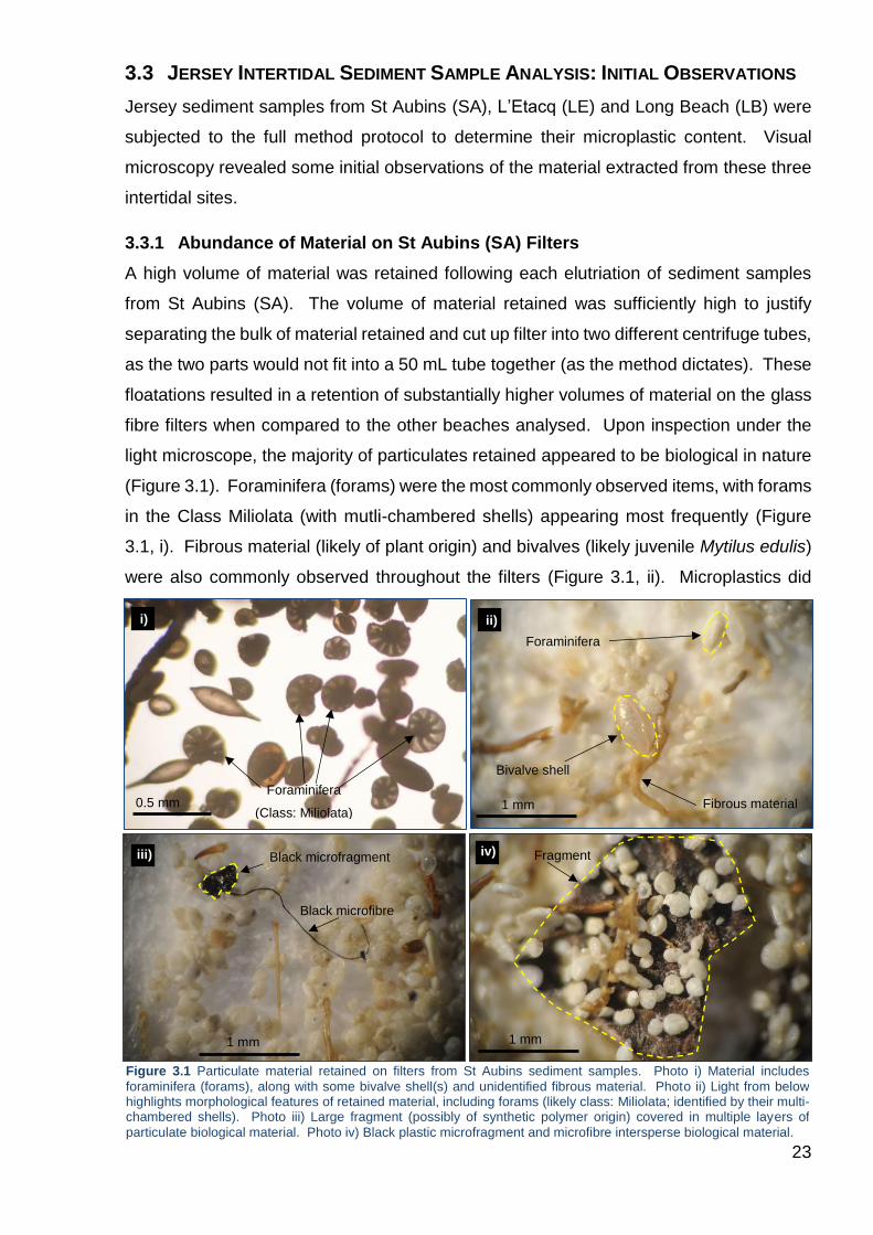
3.3 JERSEY INTERTIDAL SEDIMENT SAMPLE ANALYSIS: INITIAL OBSERVATIONS
Jersey sediment samples from St Aubins (SA), L’Etacq (LE) and Long Beach (LB) were
subjected to the full method protocol to determine their microplastic content. Visual
microscopy revealed some initial observations of the material extracted from these three
intertidal sites.
3.3.1 Abundance of Material on St Aubins (SA) Filters
A high volume of material was retained following each elutriation of sediment samples
from St Aubins (SA). The volume of material retained was sufficiently high to justify
separating the bulk of material retained and cut up filter into two different centrifuge tubes,
as the two parts would not fit into a 50 mL tube together (as the method dictates). These
floatations resulted in a retention of substantially higher volumes of material on the glass
fibre filters when compared to the other beaches analysed. Upon inspection under the
light microscope, the majority of particulates retained appeared to be biological in nature
(Figure 3.1). Foraminifera (forams) were the most commonly observed items, with forams
in the Class Miliolata (with mutli-chambered shells) appearing most frequently (Figure
3.1, i). Fibrous material (likely of plant origin) and bivalves (likely juvenile Mytilus edulis)
were also commonly observed throughout the filters (Figure 3.1, ii). Microplastics did
Figure 3.1 Particulate material retained on filters from St Aubins sediment samples. Photo i) Material includes
foraminifera (forams), along with some bivalve shell(s) and unidentified fibrous material. Photo ii) Light from below highlights morphological features of retained material, including forams (likely class: Miliolata; identified by their multi-chambered shells). Photo iii) Large fragment (possibly of synthetic polymer origin) covered in multiple layers of
particulate biological material. Photo iv) Black plastic microfragment and microfibre intersperse biological material.
ii)
1 mm
Bivalve shell
Fibrous material
Foraminifera
i)
0.5 mm Foraminifera
(Class: Miliolata)
iv)
1 mm
Fragment iii)
1 mm
Black microfibre
Black microfragment
24
appear to be present (Figure 3.1, iii), however, the sheer volume of material created an
issue with overlap of particulates (Figure 3.1, iv). This was deemed likely to result in a
number of microplastics being missed from the particulate count. In addition, it was
difficult to differentiate forams and other biological material from microplastics without
using further separation techniques or more advanced microscopy techniques. Therefore
SA samples were unable to be analysed further to determine their microplastic content.
3.3.2 Total Counts of Particles on Filters
Particles extracted from Long Beach (LB) and L’Etacq (LE) sediment samples were
visually sorted following the extraction of microplastics from sediment samples using the
amended method. Microplastics were observed under a light dissection microscope and
assigned a code using the SCS System (detailed in section 2.4). A photographic
catalogue was recorded for each filter observed under the microscope. Microplastics that
looked to be close to or above 1 mm were measured to confirm their size and allow
microplastics to be split into two size fractions; large microplastics (MP, 1 – 5 mm) and
mini-microplastics (MMP, < 1 mm).
An initial count of microplastics included small fragments of indiscernible colour (< 100
μm), which were listed as MMP/MFR/DK. Following this initial count, the total number of
microplastics observed across the two beaches was 18,574 for 2 kg of sediment. The
total for 1 kg of LB sediment was 11,571 microplastics, and for 1 kg of LE sediment was
7,002 microplastics. The two repeats for LB yielded very different counts, with 8,929
particles in LB1 and 2,642 particles in LB2 (500 g sediment each), whereas the two
repeats for LE yielded similar results (3,775 and 3,227 particles in LE1 and LE2,
respectively, from 500 g sediment). However, the characteristics of the particulates that
had been labelled MMP/MFR/DK were difficult to distinguish, on account of their small
size. This made it very difficult to rule out biological or mineral origin and verify synthetic
polymer origin for these fragments. MMP/MFR/DK were therefore removed from further
analyses, and the above totals were disregarded due to ambiguity of data for
microplastics < 100 μm. The total counts were recalculated for microplastics > 100 μm
to reduce ambiguity and improve the reliability of the data. The results of this secondary
count revealed a total count of 2,827 microplastics extracted from 2 kg sediment across
both beaches. The total for 1 kg of LB sediment was 1,473 microplastics, and for 1 kg of
LE sediment was 1,354 microplastics. The two repeats for LB yielded different counts,
with 849 microplastics in LB1 and 624 microplastics in LB2 (500 g sediment each).
Similarly, the two repeats for LE yielded counts of 574 microplastics in LE1 and 780
microplastics in LE2 (500 g sediment each).
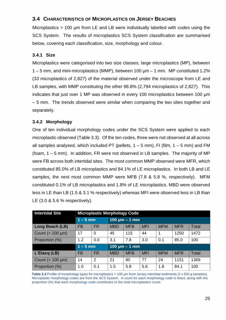
25
3.4 CHARACTERISTICS OF MICROPLASTICS ON JERSEY BEACHES
Microplastics > 100 μm from LE and LB were individually labelled with codes using the
SCS System. The results of microplastics SCS System classification are summarised
below, covering each classification, size, morphology and colour.
3.4.1 Size
Microplastics were categorised into two size classes; large microplastics (MP), between
1 – 5 mm, and mini-microplastics (MMP), between 100 μm – 1 mm. MP constituted 1.2%
(33 microplastics of 2,827) of the material observed under the microscope from LE and
LB samples, with MMP constituting the other 98.8% (2,794 microplastics of 2,827). This
indicates that just over 1 MP was observed in every 100 microplastics between 100 μm
– 5 mm. The trends observed were similar when comparing the two sites together and
separately.
3.4.2 Morphology
One of ten individual morphology codes under the SCS System were applied to each
microplastic observed (Table 3.3). Of the ten codes, three were not observed at all across
all samples analysed, which included PT (pellets, 1 – 5 mm), FI (film, 1 – 5 mm) and FM
(foam, 1 – 5 mm). In addition, FR were not observed in LB samples. The majority of MP
were FB across both intertidal sites. The most common MMP observed were MFR, which
constituted 85.0% of LB microplastics and 84.1% of LE microplastics. In both LB and LE
samples, the next most common MMP were MFB (7.8 & 5.8 %, respectively). MFM
constituted 0.1% of LB microplastics and 1.8% of LE microplastics. MBD were observed
less in LE than LB (1.5 & 3.1 % respectively) whereas MFI were observed less in LB than
LE (3.0 & 5.6 % respectively).
Intertidal Site Microplastic Morphology Code
1 – 5 mm 100 μm – 1 mm
Long Beach (LB) FB FR MBD MFB MFI MFM MFR Total
Count (> 100 μm) 17 0 45 115 44 1 1250 1472
Proportion (%) 1.2 0.0 3.1 7.8 3.0 0.1 85.0 100
1 – 5 mm 100 μm – 1 mm
L’Etacq (LB) FB FR MBD MFB MFI MFM MFR Total
Count (> 100 μm) 14 2 21 80 77 24 1151 1369
Proportion (%) 1.0 0.1 1.5 5.8 5.6 1.8 84.1 100
Table 3.3 Profile of morphology types for microplastics > 100 μm from Jersey intertidal sediments (2 x 500 g samples).
Microplastic morphology codes are from the SCS System. A count for each morphology code is listed, along with the
proportion (%) that each morphology code contributes to the total microplastics count.
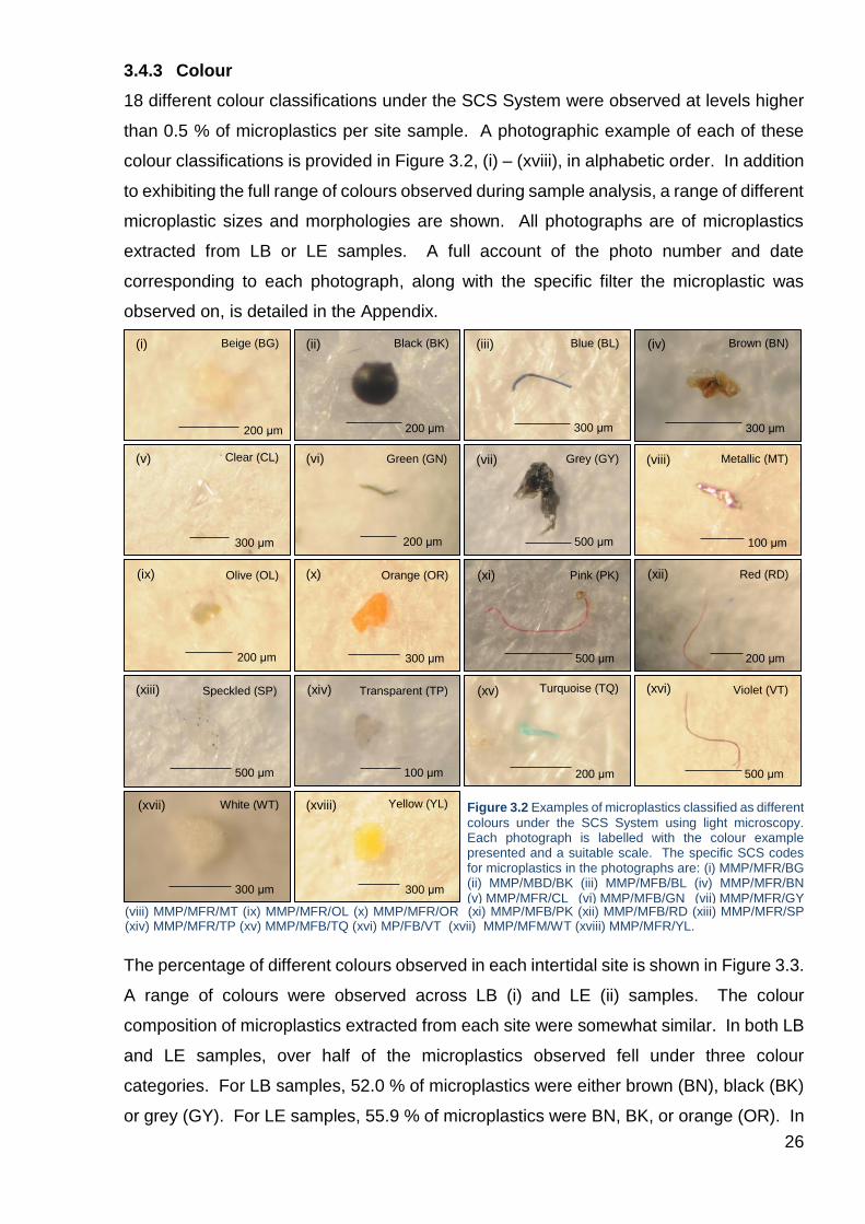
26
3.4.3 Colour
18 different colour classifications under the SCS System were observed at levels higher
than 0.5 % of microplastics per site sample. A photographic example of each of these
colour classifications is provided in Figure 3.2, (i) – (xviii), in alphabetic order. In addition
to exhibiting the full range of colours observed during sample analysis, a range of different
microplastic sizes and morphologies are shown. All photographs are of microplastics
extracted from LB or LE samples. A full account of the photo number and date
corresponding to each photograph, along with the specific filter the microplastic was
observed on, is detailed in the Appendix.
The percentage of different colours observed in each intertidal site is shown in Figure 3.3.
A range of colours were observed across LB (i) and LE (ii) samples. The colour
composition of microplastics extracted from each site were somewhat similar. In both LB
and LE samples, over half of the microplastics observed fell under three colour
categories. For LB samples, 52.0 % of microplastics were either brown (BN), black (BK)
or grey (GY). For LE samples, 55.9 % of microplastics were BN, BK, or orange (OR). In
(iii)
300 μm
(ii)
200 μm
(i)
200 μm 300 μm
(iv)
(v)
300 μm 200 μm
(vi)
200 μm
(ix)
(viii)
100 μm
(x)
300 μm
(xi)
500 μm
(xii)
200 μm
(xiii)
500 μm
(xiv)
100 μm
(vii)
500 μm
(xv)
200 μm
(xvi)
500 μm
(xvii)
300 μm
(xviii)
300 μm
Figure 3.2 Examples of microplastics classified as different
colours under the SCS System using light microscopy. Each photograph is labelled with the colour example presented and a suitable scale. The specific SCS codes for microplastics in the photographs are: (i) MMP/MFR/BG (ii) MMP/MBD/BK (iii) MMP/MFB/BL (iv) MMP/MFR/BN (v) MMP/MFR/CL (vi) MMP/MFB/GN (vii) MMP/MFR/GY
Beige (BG) Black (BK) Blue (BL) Brown (BN)
Clear (CL) Green (GN) Grey (GY) Metallic (MT)
Red (RD)
Violet (VT)
Pink (PK) Orange (OR) Olive (OL)
Speckled (SP) Transparent (TP) Turquoise (TQ)
Yellow (YL) White (WT)
(viii) MMP/MFR/MT (ix) MMP/MFR/OL (x) MMP/MFR/OR (xi) MMP/MFB/PK (xii) MMP/MFB/RD (xiii) MMP/MFR/SP (xiv) MMP/MFR/TP (xv) MMP/MFB/TQ (xvi) MP/FB/VT (xvii) MMP/MFM/WT (xviii) MMP/MFR/YL.
27
Figure 3.3 Percentage of different colours observed in microplastics > 100 μm extracted from Jersey intertidal sediments
LB and LE. (i) Colours of 1,473 microplastics extracted from LB sediment samples (2 x 500 g). Other category includes: opaque (OP), charcoal (CH), metallic (MT) and purple (PR). (ii) Colours of 1,354 microplastics from LE sediment samples (2 x 500 g). Other category includes: olive (OL), green (GN), violet (VT), purple (PR), opaque (OP), and charcoal (CH).
Long Beach (LB)
L’Etacq (LE)
(i)
(ii)
28
both LB and LE samples, BN was the most commonly observed colour (20.3 & 30.1 %),
followed by BK (18.1 & 14.6 %). Turquoise (TQ) and red (RD) microplastics constituted
similar proportions in LB and LE samples, with 1.3 & 1.7 % TQ and 1.4 & 1.3 % RD
microplastics observed across the two sites. Common rare colours observed in both sites
(‘Other’: < 0.5 % of site samples) were opaque (OP), charcoal (CH), and purple (PR).
There were also some differences observed between LB and LE samples. More than
double the proportion microplastics were blue in LB compared to LE (10.9 and 5.3 %).
The difference in proportion of white microplastics was even more pronounced,
constituting 4.8 % of LE microplastics and 1.1 % of LB microplastics. In addition, whilst
abundance of each colour did not differ substantially and was generally similar between
sites, the order of colours, from most common to least common, was different in each site
(colours are listed in order according to % composition in Figure 3.3 (i) and (ii)).
3.4.4 Size and Characteristics of Large Microplastics (MP)
MP constituted 1.2 % of the material observed under the microscope from LB and LE
samples (Table 3.3). Of these MP, most were fibres of various colours (93.9 %) and the
others were brown fragments (6.1 %).
Sample Description SCS Code Size (mm)
Sample Description SCS Code Size (mm)
Long Beach (LB) L’Etacq (LE)
LB2 C2 Black fibre MP/FB/BK 1.053 LE1 C2 Black fibre MP/FB/BK 1.236
LB1 C2 Blue fibre MP/FB/BL 1.001 LE1 C1 Blue fibre MP/FB/BL 1.177
LB2 C1 Blue fibre MP/FB/BL 1.130 LE1 C2 Blue fibre MP/FB/BL 1.276
LB2 C1 Blue fibre MP/FB/BL 1.188 LE1 C2 Blue fibre MP/FB/BL 1.291
LB2 C1 Blue fibre MP/FB/BL 1.280 LE1 C2 Blue fibre MP/FB/BL 1.339
LB2 C2 Blue fibre MP/FB/BL 1.287 LE1 C1 Blue fibre MP/FB/BL 1.886
LB1 C1 Blue fibre MP/FB/BL 1.325 LE1 C1 Brown fragment MP/FR/BN 2.846
LB2 C2 Blue fibre MP/FB/BL 1.728 LE1 C1 Brown fragment MP/FR/BN 1.025
LB2 C2 Blue fibre MP/FB/BL 1.812 LE1 C2 Grey fibre MP/FB/GY 2.635
LB2 C2 Blue fibre MP/FB/BL 2.020 LE2 C2 Pink fibre MP/FB/PK 1.006
LB2 C2 Green fibre MP/FB/GN 2.751 LE1 C1 Purple fibre MP/FB/PR 2.914
LB2 C2 Green fibre MP/FB/GN 3.108 LE2 C2 Turquoise fibre MP/FB/TQ 1.160
LB2 C1 Grey fibre MP/FB/GY 1.422 LE2 C2 Turquoise fibre MP/FB/TQ 1.286
LB2 C2 Pink fibre MP/FB/PK 1.223 LE2 C1 Turquoise fibre MP/FB/TQ 2.329
LB1 C1 Pink fibre MP/FB/PK 1.234 LE1 C1 Violet fibre MP/FB/VT 1.002
LB2 C2 Pink fibre MP/FB/PK 1.702 LE1 C1 Violet fibre MP/FB/VT 2.503
LB1 C1 Turquoise fibre MP/FB/TQ 1.335
Table 3.4 Detailed catalogue of microplastics > 1 mm. Microplastics are listed under the intertidal sediment they were
extracted from, with the specific sample (LB1, LB2, LE1 or LE2) and #centrifugation (C1 or C2) given in the left-hand column. The description gives the same information as the SCS code in a more digestible format in the centre two columns. Each microplastic was measured along the longest diameter (fragment) or length (fibre) three times using
ImageJ, with the mean average listed in the right-hand column.
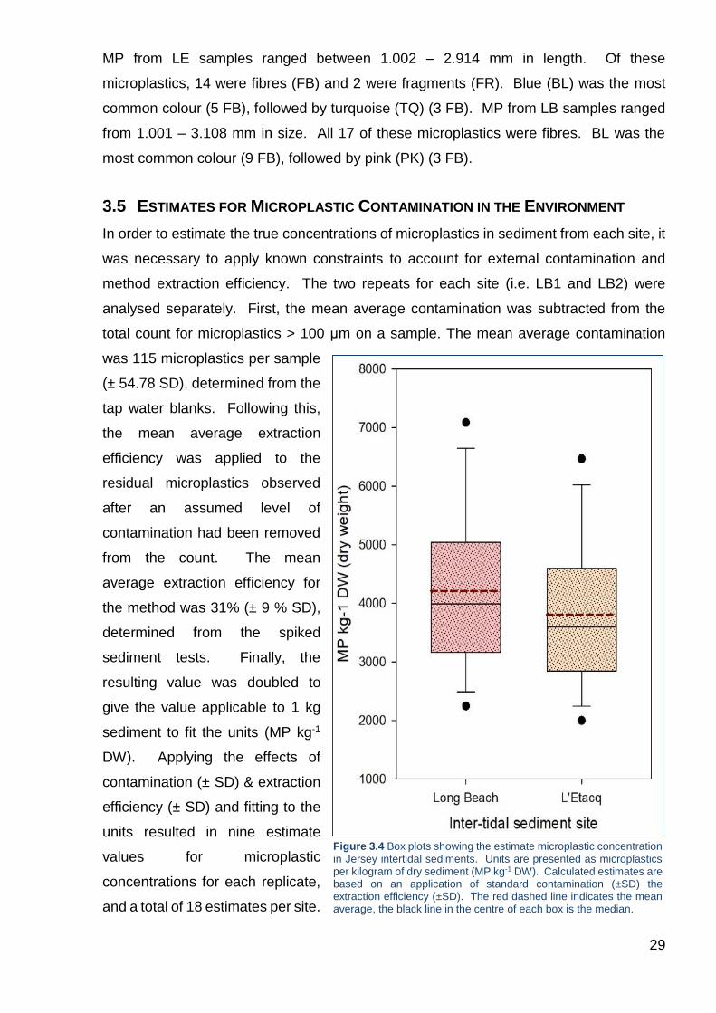
29
MP from LE samples ranged between 1.002 – 2.914 mm in length. Of these
microplastics, 14 were fibres (FB) and 2 were fragments (FR). Blue (BL) was the most
common colour (5 FB), followed by turquoise (TQ) (3 FB). MP from LB samples ranged
from 1.001 – 3.108 mm in size. All 17 of these microplastics were fibres. BL was the
most common colour (9 FB), followed by pink (PK) (3 FB).
3.5 ESTIMATES FOR MICROPLASTIC CONTAMINATION IN THE ENVIRONMENT
In order to estimate the true concentrations of microplastics in sediment from each site, it
was necessary to apply known constraints to account for external contamination and
method extraction efficiency. The two repeats for each site (i.e. LB1 and LB2) were
analysed separately. First, the mean average contamination was subtracted from the
total count for microplastics > 100 μm on a sample. The mean average contamination
was 115 microplastics per sample
(± 54.78 SD), determined from the
tap water blanks. Following this,
the mean average extraction
efficiency was applied to the
residual microplastics observed
after an assumed level of
contamination had been removed
from the count. The mean
average extraction efficiency for
the method was 31% (± 9 % SD),
determined from the spiked
sediment tests. Finally, the
resulting value was doubled to
give the value applicable to 1 kg
sediment to fit the units (MP kg-1
DW). Applying the effects of
contamination (± SD) & extraction
efficiency (± SD) and fitting to the
units resulted in nine estimate
values for microplastic
concentrations for each replicate,
and a total of 18 estimates per site.
Figure 3.4 Box plots showing the estimate microplastic concentration
in Jersey intertidal sediments. Units are presented as microplastics per kilogram of dry sediment (MP kg-1 DW). Calculated estimates are based on an application of standard contamination (±SD) the extraction efficiency (±SD). The red dashed line indicates the mean average, the black line in the centre of each box is the median.
30
These data are presented for each site as box plots (Figure 3.4). The range of values
obtained for LB was 2,248.2 – 7,081.1 MP kg-1 DW, whilst the range for LE was 2,000.7
– 6,467.2 MP kg-1 DW. The mean average concentration of microplastics (100 μm – 5
mm) in LB sediments was estimated to be higher than that of LE sediments. The mean
average for LB was 4,209 (± 1,377) MP kg-1 DW and the mean average for LE was 3,806
(± 1,258) MP kg-1 DW.
3.6 GRAIN SIZE ANALYSIS AND SAMPLE LOSS
Grain size analysis was carried out for all sediments put through elutriation (Table 3.5).
This included three sediment samples (collected at Hayling Island) used for spiked
sediment tests with three different polymers (PA, PS and PVC), and 2 repeat samples
from each of the three Jersey intertidal sites analysed (LB, LE and SA). Sediments were
sieved through a 5 mm mesh prior to elutriation and some material > 5 mm was retained
for most samples. Therefore grain size analysis results would have been slightly different
if conducted before elutriation. However, the primary purpose of grain size analysis was
to quantify the grain size of sediments as they would have been during elutriation, not as
it was when collected from the environment. Additional contamination from stacked
sieves and other equipment is a further reason this analysis was not carried out before
elutriation. Spiked sediment samples (SPA/SPS/SPVC) were given the description
‘moderately well-sorted, fine sand’, and were very similar in composition, with close mean
grain sizes and % sand and mud content. This was expected, as these three samples
were sourced from the same location. Similarly, the repeat samples for each Jersey
intertidal site (LB1/LB2, LE1/LE2, SA1/SA2) had similar mean grain sizes and sand/mud
Table 3.5 Grain size analysis results. Samples from the spiked sediment tests are prefixed with ‘S’, followed by the
abbreviation for the polymer used to spike the sample. Samples from Jersey intertidal sites are prefixed with the site abbreviation, followed by the number repeat. The arithmetic (μm) and logarithmic (ϕ) mean grain size is provided for each sample, along with sand and mud content (%), overall sample loss from elutriation and sieving (%), and an overall sediment description.
Sediment
Sample
Mean grain size Sand (%) Mud (%) Loss (%) Overall sediment description
μm ϕ
SPA 191.3 2.341 100.0 0.0 1.8 Moderately well sorted, fine sand
SPS 192.0 2.355 99.9 0.1 1.5 Moderately well sorted, fine sand
SPVC 188.2 2.365 99.9 0.1 3.1 Moderately well sorted, fine sand
LB1 329.0 1.751 100.0 0.0 1.3 Moderately sorted, medium sand
LB2 319.2 1.768 100.0 0.0 2.4 Moderately sorted, medium sand
LE1 201.9 2.355 100.0 0.0 51.6 Very well sorted, fine sand
LE2 205.5 2.328 100.0 0.0 2.8 Very well sorted, fine sand
SA1 104.1 3.309 98.2 1.8 11.2 Very well sorted, very fine sand
SA2 104.5 3.301 98.6 1.4 18.9 Very well sorted, very fine sand
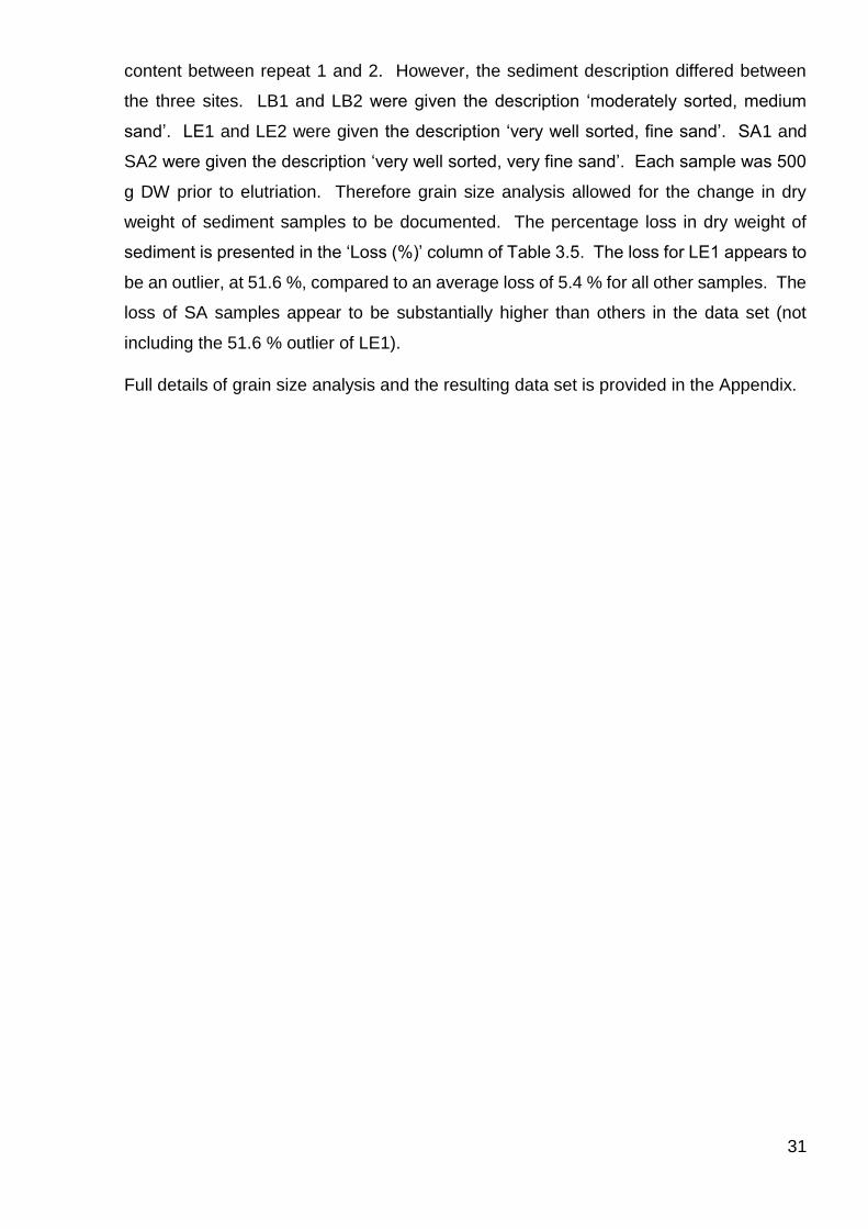
31
content between repeat 1 and 2. However, the sediment description differed between
the three sites. LB1 and LB2 were given the description ‘moderately sorted, medium
sand’. LE1 and LE2 were given the description ‘very well sorted, fine sand’. SA1 and
SA2 were given the description ‘very well sorted, very fine sand’. Each sample was 500
g DW prior to elutriation. Therefore grain size analysis allowed for the change in dry
weight of sediment samples to be documented. The percentage loss in dry weight of
sediment is presented in the ‘Loss (%)’ column of Table 3.5. The loss for LE1 appears to
be an outlier, at 51.6 %, compared to an average loss of 5.4 % for all other samples. The
loss of SA samples appear to be substantially higher than others in the data set (not
including the 51.6 % outlier of LE1).
Full details of grain size analysis and the resulting data set is provided in the Appendix.
32
4 DISCUSSION
4.1 MICROPLASTICS IN JERSEY INTERTIDAL SEDIMENTS
The ratio of the two size fractions of microplastics (MP:MMP) was the remarkably similar
for LB and LE sediments (3:247 approx. for both). This could be indicative of the presence
of a greater number of microplastics in the smaller size category (MMP) in the
environment, which is consistent with the literature (see Table 1.1). However, there was
a considerable difference in extraction efficiency between MP and MMP during the spiked
sediment tests (22 and 41 %, respectively). This is likely to have reduced the amount of
MP extracted from sediment samples and therefore contributed to the pronounced
difference in counts for each size category.
Primary microplastics (PT and MBD) were rare in both sites, with the majority of
microplastics appearing to be of secondary origin, with most of these in the form of MFR
or MFB. Secondary microplastics occur as a result of degradation from larger plastic
items. This suggests that the majority of microplastics found in Jersey sediments are the
result of weathering of post-consumer plastic items present in the marine environment.
The microplastics colour profiles for each site were also somewhat similar, suggesting
that a similar assemblage of microplastics exist in sediments to the East and West of the
island. The majority of microplastics observed in both sites were brown, followed by
black. These colours are common to natural materials (biological and mineral) in the
marine environment. For example, granite is particularly common in Jersey sediments
and can be black in colour. This could suggest some level of misidentification during
visual sorting. However, even if a marginal portion these particles are of synthetic
polymer origin, this may pose a considerable threat to marine species, as black
microplastics have been shown to be preferentially ingested by marine species compared
to other colours (Ory et al., 2018).
Overall, the microplastics extracted from Jersey intertidal sediments appeared to be
similar for western (LE) and eastern (LB) beaches. The estimate microplastic
concentrations for LB and LE were marginally different (mean average 4,209 ± 1,377 MP
kg-1 DW and 3,806 ± 1,258 MP kg-1 DW, respectively). However, as these estimates
were subject to two major assumptions (external contamination levels and method
extraction efficiency) the range of estimated values varied greatly. Thus it was difficult to
quantify the significance of the marginal differences observed. In addition, when the
estimated microplastic concentrations for intertidal sites were compared to the literature,
33
it was found that they were one order of magnitude (or even two) in excess of the
concentrations from comparable studies. For example, two studies that quantified the
microplastic concentrations of marine sediments in Belgium, and considered a similar
size range of microplastics to this study (38 μm – 1 mm), reported concentrations at 166.7
MP kg-1 DW (harbour), 92.8 MP kg-1 DW (beach), 17.6 MP kg-1 DW (high tide line) and
9.2 MP kg-1 DW (low tide line) (Claessens et al., 2011; Van Cauwenberghe et al., 2013a).
Similarly, the microplastic concentrations of Slovenian marine sediments have been
recorded at 177.8 MP kg-1 DW (beach) and 170.4 MP kg-1 DW (Infralittoral) for
microplastics between 250 μm – 5 mm. All of these reported concentrations are at least
one order of magnitude lower than the estimates for Jersey intertidal sites. A study by
Frère et al. (2017) considered microplastics between 0.7 μm – 1 mm and found
concentrations of 0.97 MP kg-1 DW in subtidal sediments from the Bay of Brest. This is
very low compared to the results found for Jersey samples, particularly considering that
Frère et al. (2017) included a lower limit for microplastic size that was 2 orders of
magnitude smaller than the lower limit for LB and LE microplastics (0.7 μm vs 100 μm).
Conversely, the differences observed between the Bay of Brest and Jersey sediments
could be due to the different site sources; subtidal and intertidal, respectively.
Microplastics, in particular low density polymers, are known to accumulate on beaches
and thus higher concentrations of microplastics are generally found in beach sediments
compared to subtidal sediments (Zhang, 2017). One study from Canada with comparable
results reported microplastic concentrations on a Nova Scotia beach between 2,000 –
8,000 MP kg-1 (Mathalon and Hill, 2014). However, similarly to Frère et al. (2017),
Mathalon and Hill (2014) consider a lower size limit for microplastics that is 2 orders of
magnitude smaller than the lower limit for LB and LE microplastics (0.8 μm vs 100 μm),
thus a greater concentration of microplastics, and not a comparable value, would be
expected. These comparisons with data sourced from recent literature call into question
the validity and robustness of the data obtained for Jersey intertidal sediments in this
study.
With this in mind, it is of note that the amended method had a number of limitations,
identified throughout the method optimisation and sample analysis phases of the
research. These impacted on the validity of the data, which made it difficult to draw robust
conclusions from the results, due to the level of implicit and observed variance. Therefore
the remainder of this section is dedicated to a discussion around the various method
limitations and suggestions for improvements where relevant.
34
4.2 SOURCES OF CONTAMINATION IN THE LABORATORY
Although steps were taken to minimise contamination (see section 2.6), samples were
nonetheless exposed to varying levels of contamination throughout the process of
laboratory analysis. This was evident from the results of blanks carried out with tap water,
seawater and RO water, with filters from every blank containing microplastics in varying
concentrations. It was assumed, prior to the blanks being carried out, that RO water
would result in the cleanest blanks. This is because RO water is the purest water source
of the three tested mediums and microplastics have been found at trace levels in tap
water (Mintenig et al., 2019; Pivokonsky et al., 2018). However, the results indicated
otherwise, with tap water resulting in marginally purer blanks than RO water, overall.
These results suggested that any microplastics within tap water did not impact on the
overall contamination levels observed between tap water and RO water. The base levels
of contamination observed across tap water and RO water blanks are therefore likely to
originate primarily from laboratory surfaces, equipment and airbourne microplastics.
Potential sources of microplastic contamination included blue fibres leached from the
nylon rope that held the elutriation column in place, grey PVC fragments from the custom-
made PVC elutriation column, airbourne synthetic fibres, and microplastics in dust that
had settled on equipment, hoses and laboratory worktop surfaces.
Microplastics > 1 mm from
blank and sample filters were
compared (Table 4.1). The
morphology of each MP
observed was almost
exclusively fibres (FB) for both
the blanks and samples. In
addition, total counts for each
of the blanks and analyses
were not markedly different.
The similarity to the blanks suggests that the majority of fibres observed on sample
analysis filters originated from external contamination rather than from the environmental
sample.
In addition, microscopic materials other than plastics may have been mistaken for
microplastics under the microscope. For example, microscopic pieces of the steel 38 μm
pore size filters could have been released following them being cut and placed into ZnCl2
Blank or sample analysis name
MP Count (> 1 mm)
Morphologies observed
Size Range (mm)
B1 9 FB 1.12 – 5.94
B2 2 FB 1.14 – 1.20
B3 6 FB 1.00 – 1.87
LB1 4 FB 1.00 – 1.34
LB2 13 FB 1.13 – 3.11
LE1 12 FB, FR 1.00 – 2.91
LE2 4 FB 1.00 – 1.29
Table 4.1 Comparison of microplastics > 1 mm observed on filters from tap
water blanks and sample analyses. The total count of microplastics > 1 mm is provided along with the morphology codes for microplastics observed and the size range (measured using ImageJ).
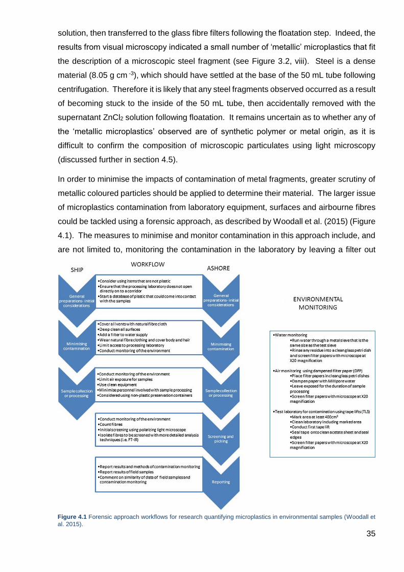
35
solution, then transferred to the glass fibre filters following the floatation step. Indeed, the
results from visual microscopy indicated a small number of ‘metallic’ microplastics that fit
the description of a microscopic steel fragment (see Figure 3.2, viii). Steel is a dense
material (8.05 g cm -3), which should have settled at the base of the 50 mL tube following
centrifugation. Therefore it is likely that any steel fragments observed occurred as a result
of becoming stuck to the inside of the 50 mL tube, then accidentally removed with the
supernatant ZnCl2 solution following floatation. It remains uncertain as to whether any of
the ‘metallic microplastics’ observed are of synthetic polymer or metal origin, as it is
difficult to confirm the composition of microscopic particulates using light microscopy
(discussed further in section 4.5).
In order to minimise the impacts of contamination of metal fragments, greater scrutiny of
metallic coloured particles should be applied to determine their material. The larger issue
of microplastics contamination from laboratory equipment, surfaces and airbourne fibres
could be tackled using a forensic approach, as described by Woodall et al. (2015) (Figure
4.1). The measures to minimise and monitor contamination in this approach include, and
are not limited to, monitoring the contamination in the laboratory by leaving a filter out
Figure 4.1 Forensic approach workflows for research quantifying microplastics in environmental samples (Woodall et
al. 2015).
36
during sample analysis, wearing only cotton laboratory coats and clothing, and covering
all vents with natural fibre cloth. In addition, clean air filters have been shown to reduce
airbourne microfibre contamination in the laboratory by up to 96.5 % (Wesch et al., 2017).
Efforts to wear only 100 % cotton laboratory coats and clothing during analysis of samples
is commonplace in the more recent studies quantifying microplastics in the environment
(Frère et al., 2017; Steer et al., 2017). In addition, the method could be amended to
reduce the amount of plastic equipment used and thereby minimise contamination further.
For example, the PVC elutriation column could be replaced with a custom-made metal or
glass elutriation column.
4.3 SAMPLE LOSS
The amount of sediment collected from intertidal sites was specified at 500 g per sample,
with 500 g DW required for each sediment analysis. As part of sample preparation,
sediments were dried in separate containers to remove excess water content. This
resulted in 63 % of the intertidal sediment samples prepared weighing less than 500 g
after drying (see Appendix, Table i). For the two replicates analysed for each site, SA
and LE samples were > 500 g, but one LB sample was < 500 g once dried (490.4 g DW).
This sample was topped up with excess dry sediment from the other sample collected
from LB (519.4 g DW). The mean average weight loss per sample after drying for all
samples prepared was 14.3 %, with a maximum loss of 20.9 %. With this in mind, it would
be advised for future research that additional sediment (perhaps 25 % extra, so 625 g
minimum if collecting 500 g) is collected in the field in order to ensure the sample size is
sufficient to carry out analysis in the laboratory.
As part of the grain size analysis, the total weight of sediment samples that had been
analysed was compared to the original 500 g weight to calculate the % loss of sediment
following elutriation. All samples reduced in weight to some degree. A small portion of
this loss could be attributed to the loss of lighter material (including microplastics) via
elutriation. This appears to have impacted SA samples (SA1 and SA2), which were
observed to retain higher volumes of material on the retaining sieve. SA1 and SA2
experienced weight losses of 11.2 and 18.9 %, respectively compared to an average loss
of 2.2 % in all other samples (excluding an outlier of 51 % loss). However, there are also
other steps where loss could have occurred throughout the method. For example, the
mesh supporting the sediment at the base of the column had 38 μm apertures, which
would have allowed sediment grains < 38 μm to escape at the base of the column. In
addition, as the supporting mesh was removed, cleaned and then replaced between
37
elutriations, it is possible that the sieve could have been replaced ineffectively, leaving a
gap for sediment to escape. It was found that one of the samples had reduced in weight
by 51 % (LE1), which was likely due to a misplacement of the base sieve mesh.
In addition to sediment loss, there were other steps where microplastics in the sediment
could have been lost. All samples were dried prior to elutriation, with some dried in an
oven at 60 °C and some dried in an autoclave. After drying was complete, it was noted
that the standard temperature of the autoclave was approximately 120 °C. This could
have resulted in the melting together of microplastics consisting of polymers with a low
melting temperature (i.e. some grades of PE have a melting temperature as low as 80
°C). The presence of microplastics with lower melting temperatures would likely reduce
the overall count of microplastics extracted from a sample. This would only be applicable
to LE and SA samples, which were dried in the autoclave, and not to LB samples, which
were dried in the oven.
During elutriation, microplastics could have become stuck to the inside of the PVC column
due to static interactions. In addition, microplastics which exited the column via
supernatant water may have stuck to the retainer filter edges or column outflow lip.
Between elutriation and floatation, filters were stored in aluminium foil. Despite the
removal of excess water from the filters by dabbing the clean side on blue roll prior to
being wrapped, the foil degraded quickly on account of the residual moisture present on
the filters. This may have resulted in a slight loss of solids retained on the elutriation
filters due to gaps in the foil wrap caused by degradation. In addition, the preparation of
filters for floatation by cutting into 0.5 – 1 mm squares also could have resulted in the loss
of microplastics. During floatation, microplastics may have become trapped inside the
glass pipette used to transfer the surface layer to the filter. They could have also become
stuck to the sides of the Büchner funnel during vacuum filtration, despite rinsing with RO
water to minimise this. In addition, microplastics may have remained within ZnCl2 solution
or stuck to the edges of the centrifuge tube near the surface of the solution.
Further measures could be taken to overcome some of these loss steps throughout the
method. This includes securing the base sieve filter in place with bolts before adding
sediment to the PVC column, which would minimise the loss of sediment during
elutriation. Fewer transfer steps would also reduce the potential for sample loss. For
example, instead of wrapping filters in foil then carrying out floatation at a later stage,
floatation could be carried out immediately after elutriation to remove the need for
wrapping filters between these two method steps. Alternatively, other methods involving
38
a single step for microplastics extraction from sediments could be considered, such as
the use of a Sediment-Microplastic Isolation (SMI) unit, proposed by Coppock et al.
(2017). This technique involves a single step floatation using ZnCl2 solution, thus
reducing the potential loss steps through transfer of solids to different containers.
4.4 LOW METHOD EXTRACTION EFFICIENCY
The spiked sediment tests resulted in varied extraction efficiencies across size range,
morphology and polymer type (22 – 41 %). Compared to the results of spiked sediment
tests presented in Claessens et al. (2013) (98 – 100 %), these results indicated that the
amended method had a very low method extraction efficiency (mean average 31 %). This
was substantially lower than the target extraction efficiency of > 90 % that was set as an
objective of this study. The issues around extraction efficiency arguably presented the
most considerable method limitations, as the efficiency was not only low, but had
substantial variation between size and polymer type. This meant that the microplastics
profile observed on the filters following extraction from intertidal sediments was not likely
to be fully representative of the microplastics in the environment.
PA fibres were recovered from spiked sediment samples at a higher % than fragments of
PVC and PS (41 % vs 30 % and 23 %, respectively). This suggests that microplastics of
different morphology types and polymers were recovered from sediment samples at
different extraction efficiencies. Also, as mentioned previously, microplastics between 1
– 5 mm were recovered at around half the % of microplastics between 100 μm – 1 mm
(22 and 41 %, respectively). This likely impacted the results of sample analysis by
underestimating the contribution of large microplastics to microplastic contamination in
sediments. This particular method involving elutriation was therefore deemed to be
incompatible with the extraction of microplastics > 1 mm.
Ideally, the extraction efficiency for microplastics should be consistently > 90% for
microplastics of varying characteristics (i.e. morphology, polymer, size) found in the
environment. Further method optimisation is required to try and achieve a higher
extraction efficiency of microplastics from sediments. This could include different aeration
stone setups, and/or different water flow rates for elutriation. Another suggested
amendment to the method would be to change the initial sieve, used for sorting sediments
prior to elutriation, back to 1 mm, as in Claessens et al. (2013). Following this, the
sediment sample < 1 mm would be run through the method as described (elutriation,
floatation, microscopy). The sediment > 1 mm retained on the sieve would then be sieved
through a 5 mm mesh to remove larger debris and put through floatation in high-density
39
salt solution (no elutriation necessary). In addition, more robust and varied spiked
sediment tests should be carried out to assess a wider range of polymer types (i.e. PE,
Polyethylene terephthalate; PET) and morphologies (i.e. MBD, MFI, MFM).
4.5 POTENTIAL IMPACTS OF SEDIMENT GRAIN SIZE ON METHOD SUITABILITY
Grain size analysis revealed that sediments varied in characteristics between intertidal
sites (Table 3.5). It is likely that grain size impacted on the results (or lack thereof)
obtained from SA sample analysis. SA sediments were the finest of the three Jersey
intertidal sediments analysed, assigned as ‘very well sorted, very fine sand’ following
grain size analysis (mean grain size 104.3 μm). Following elutriation and floatation, the
material extracted from SA samples was of substantially more volume than that of the
other samples, and was found to be primarily biological material (forams, bivalves, etc.).
The volume and abundance of material that was not of synthetic polymer origin rendered
analysis of these filters difficult, and thus visual sorting of microplastics was unsuccessful.
It is likely that the high-density ZnCl2 solution used during the floatation step was
sufficiently dense to float the small biological structures within the sediment such as
bivalve and foraminifera shells (Figure 3.1). In addition, grain size could have impacted
on the overall efficiency of the method. This could be confirmed through further tests
involving spiked sediment with different grain size distributions. It is important to have a
method which is relatively consistent across different grain sizes, as sediment grain size
may also impact the distribution of microplastics found in marine sediments (Martins and
Sobral, 2011).
To overcome the prevalence of non-plastic material extracted from finer sediments,
further laboratory techniques to isolate microplastics could be employed. A number of
studies have used hydrogen peroxide (H2O2) to treat samples prior to analysis in order to
remove biological material (Cole et al., 2014; Foekema et al., 2013; Mathalon and Hill,
2014; Wesch et al., 2016). However, this was demonstrated to result in incomplete
dissolution of biological tissue and a significant loss of microplastics from samples (Nuelle
et al., 2014). The use of technical grade enzymes, including proteinase, chitinase,
cellulose and lipase, could offer a more effective approach to remove biological content
of sediments. For example, the Basic Enzymatic Purification Protocol (BEPP) proposed
by Löder et al. (2017), which involves several stages of enzymatic purification to remove
various types of biological material at each stage (shells, exoskeletons, cell walls, etc.).
This technique is preferable because enzymes are biological agents and thus do not
40
destroy or impact on the microplastics present with the sample, as they are not easily
impacted by biological processes.
4.6 IDENTIFICATION OF MICROPLASTICS USING LIGHT MICROSCOPY
Visual sorting using a microscope to define the type, morphology, and colour of
microplastics is one of the most common methods of microplastics identification, and is
suggested as a first step for microplastics analysis (Hidalgo-Ruz et al., 2012). This
method is cost-effective and provides some idea of the range and number of microplastics
extracted from sediment samples. Due to a lack of availability of other analytical
techniques to identify microplastics for the specific scope of this study, visual sorting using
a light microscope was used as the sole method to identify and quantify microplastics in
Jersey intertidal sediments. This presented a number of method limitations and issues.
Firstly, visual sorting was extremely time-consuming (approx. 3 – 4 hours per filter). It is
a subjective method, which is highly dependent on light levels, the person examining the
filters, and the quality and magnification of the dissection microscope. This is particularly
true with regard to identifying colour (Song et al., 2015). In addition, visual identification
does not allow for the verification of material type. This meant that polymer type could
not be confirmed for particles extracted from Jersey samples, and, more importantly, it
was not possible to ascertain that the particles visually resembling microplastics were of
synthetic polymer origin. The importance of using analytical laboratory techniques to
determine the chemical composition the particles resembling microplastics (i.e. FT-IR or
Raman spectroscopy, detailed below) was highlighted in a recent case study by Löder
and Gerdts (2015). In the case study, only 1.4% of particles that resembled microplastics
under the microscope were of synthetic polymer origin (particles between 100 – 500 μm,
approx.). The majority of other particles extracted were confirmed as quartz sand
granules, using FT-IR analysis and comparison of spectra to the IR spectrum of laboratory
quartz. Taking the visual observations into account on their own would therefore result
in error rate of 98.6 %. Even considering larger particle sizes (> 500 μm), which are
somewhat easier to categorise under the microscope, the error rate of visual sorting
reported in the literature ranges from 20 % (Eriksen et al., 2013a) to 70 % (Hidalgo-Ruz
et al., 2012). With a lack of laboratory analysis techniques available as part of the scope
of this project, it was not possible to confirm the chemical composition of particles
observed on the filters following extraction from Jersey intertidal sediments. Therefore it
is highly likely that the estimate totals for microplastics concentrations (Figure 3.4) are a
gross overestimation of microplastics in the environment. Assuming a high error rate of
41
98.6%, as presented by Löder and Gerdts (2015), the mean average estimates for LB
and LE (without standard deviation) would be altered from 4,209 MP kg-1 DW and 3,806
MP kg-1 DW, respectively, to 58.9 MP kg-1 DW and 53.3 MP kg-1 DW, respectively.
Interestingly, this is more in line with recorded concentrations for sediments published in
the literature (Table 1.1). However, it was not possible to determine the actual error rate
for microplastic identification in Jersey intertidal samples. Thus these postulations only
serve to highlight the implicit variance in the microplastic concentration estimates.
Another fundamental drawback of visual sorting is the size limitation. In this study, initial
counts included smaller particles (< 100 μm), which were listed as dark microfragments
(MMP/MFR/DK). However, later in the study, it was decided that these fragments should
not be included in the final counts, because their minuteness meant that they were unable
to be visually discriminated as microplastics with any degree of certainty. The total count
without MMP/MFR/DK was 84.8 % lower than the initial count across the two sites
(individually, the second count for LB was 87.3 % lower, and for LE was 80.7 % lower
than the initial count). Conversely to the issue of error rates described above, this
limitation could result in an underestimation of microplastics observed in Jersey
sediments, by excluding the size fraction between 38 – 100 μm.
Visual sorting of microplastics is therefore recommended to be used as a first step for
microplastics analysis only. New techniques have been developed to assist with visual
sorting, including the use of Nile red dye to quantify PE, PP, PS and nylon particles by
fluorescence (Erni-Cassola et al., 2017). However, visual sorting is only suitable for
identifying larger microplastics. Some studies suggest a particle size limit > 500 μm
(Löder and Gerdts, 2015), whilst others suggest a more conservative limit of > 1 mm
(Hidalgo-Ruz et al., 2012). Material extracted from intertidal sediment samples should be
subject to further analyses to verify synthetic polymer origin of particles observed. As
mentioned above, Fourier-Transform Infra-Red spectroscopy (FT-IR) and Raman
spectroscopy are common methods that have been used in previous studies to do this
(Elert et al., 2017). Both techniques involve obtaining a spectrum for a particle and
comparing this to a library of known synthetic polymer spectra. FT-IR is the arguably the
most reliable and straightforward method of differentiating between plastic and non-
plastic items, and is also capable of identifying particles down to a few μm (Hidalgo-Ruz
et al., 2012). Thus FT-IR is the most widely used technique across the literature
(Cincinelli et al., 2017; Kunz et al., 2016; Mohamed Nor and Obbard, 2014; Syranidou et
al., 2017; Yu et al., 2018). Raman spectroscopy recommended for particles < 20 mm in
size, as it provides higher resolution spectra (Shim et al., 2017).
42
5 SUMMARY OF FINDINGS
A method for extracting microplastics from environmental sediment samples was
developed and optimised to cover a wide size range of microplastics (100 – 5 mm).
However, the method was subject to a number of limitations. The mean average
extraction efficiency achieved using sediments spiked with microplastics was 31 %. This
was substantially lower than the target extraction efficiency of > 90 % that was set as an
objective of this study. This, along with a number of other method limitations, impacted
greatly on the data obtained from sample analysis, and made it difficult to draw any robust
conclusions with regards to microplastic contamination in Jersey intertidal sites. A
microplastic profile was outlined for the particles observed on filters, however, due to the
numerous method limitations and variance in the data, this is not likely to be realistic to
the microplastic profile found in the environment and is thus not considered an accurate
representation of microplastic contamination in Jersey intertidal sediments. Estimates for
microplastic concentrations in Jersey intertidal sediments, even taking contamination
levels into account, were at least one order of magnitude in excess of recorded
concentrations for sediments in the literature, which further supported the theory that this
data was unrealistic.
Other method limitations identified following sample analysis included microplastic
contamination in the laboratory, likely in the form of airbourne fibres, microplastic particles
on surfaces and equipment, and fragments leached from plastic equipment. This was
quantified using the results of tap water blanks. The characteristics of microplastics > 1
mm were remarkably similar between sample and blank filters, suggesting that airbourne
filters had contaminated the sample filters to some degree. There were also a number of
potential sample loss steps throughout the method for sediments and microplastics,
which could have impacted on the final counts. Finally, the visual sorting method used to
identify and quantify microplastics on filters was highly subjective. The use of an
analytical method to confirm the synthetic polymer origin of particles (i.e. FT-IR or Raman
spectroscopy) would have greatly increased the reliability of the data.
These results highlight the implicit variance in microplastics data and substantiate the
importance of clean laboratory spaces and standardised methods for the analysis of
environmental samples.
43
6 FUTURE DIRECTIONS
The field of microplastics research is a relatively recent development, and thus the
majority of techniques for the monitoring and quantification of microplastic contamination
in marine sediments are still in the preliminary stages of testing and validation. This study
demonstrates the complexities of microplastics research, with multiple variables and
limitations impacting the validity of environmental data, and attests to the importance in
working towards standardised techniques for microplastic quantification in sediments.
To further improve the specific method outlined in this study, it is recommended that:
- A forensic approach is adopted (i.e. clean air filters, cotton lab coats, monitoring)
- Non-plastic equipment be used where possible (i.e. metal elutriation column)
- 25 % extra sediment should be collected in the field to account for drying
- The elutriation column base sieve should be secured with bolts to prevent loss
- Floatation should be carried out immediately after elutriation to reduce transfer steps
- Amend the protocol for microplastics > 1 mm (sieve separation then floatation only)
- Carry out further spiked sediment tests to assess microplastics of different polymers
and morphologies, and different grain size sediments
- Optimise the aeration and water flow rate to maximise extraction efficiency
- Treat samples with enzymatic purification protocol to remove biological material
- Use FT-IR and/or Raman spectroscopy to confirm synthetic polymer origin
Alternatively, other methods for microplastics extraction from sediments could be
considered, such as the use of a Sediment-Microplastic Isolation (SMI) unit, proposed by
Coppock et al. (2017), which involves a single step floatation using ZnCl2 solution.
Overall, priority should be given to standardising the general protocol for microplastics
research to keep the impacts of contamination to a consistent minimum across studies.
The forensic approach outlined by Woodall et al. (2015) is recommended for future work
to quantify microplastics in marine sediments and other environmental samples.
44
LITERATURE CITED
Andrady, A.L., 2011. Microplastics in the marine environment. Mar. Pollut. Bull. 62, 1596–1605. https://doi.org/10.1016/j.marpolbul.2011.05.030
Barnes, D.K.A., Galgani, F., Thompson, R.C., Barlaz, M., 2009. Accumulation and fragmentation of plastic debris in global environments. Philos. Trans. R. Soc. B Biol. Sci. 364, 1985–1998. https://doi.org/10.1098/rstb.2008.0205
Baztan, J., Carrasco, A., Chouinard, O., Cleaud, M., Gabaldon, J.E., Huck, T., Jaffrès, L., Jorgensen, B., Miguelez, A., Paillard, C., Vanderlinden, J.P., 2014. Protected areas in the Atlantic facing the hazards of micro-plastic pollution: First diagnosis of three islands in the Canary Current. Mar. Pollut. Bull. 80, 302–311. https://doi.org/10.1016/j.marpolbul.2013.12.052
Besseling, E., Wegner, A., Foekema, E.M., Van Den Heuvel-Greve, M.J., Koelmans, A.A., 2013. Effects of microplastic on fitness and PCB bioaccumulation by the lugworm Arenicola marina (L.). Environ. Sci. Technol. 47, 593–600. https://doi.org/10.1021/es302763x
Blott, S.J., Pye, K., 2001. Gradistat: A Grain Size Distribution and Statistics Package for the Analysis of Unconcolidated Sediments. Earth Surf. Process. Landforms 26, 1237–1248. https://doi.org/10.1002/esp.261
Blumenröder, J., Sechet, P., Kakkonen, J.E., Hartl, M.G.J., 2017. Microplastic contamination of intertidal sediments of Scapa Flow, Orkney: A first assessment. Mar. Pollut. Bull. 124, 112–120. https://doi.org/10.1016/j.marpolbul.2017.07.009
Boucher, J., Friot, D., 2017. Primary microplastics in the oceans: A global evaluation of sources. https://doi.org/10.2305/IUCN.CH.2017.01.en
Brillant, M.G.S., MacDonald, B.A., 2000. Postingestive selection in the sea scallop, Placopecten magellanicus (Gmelin): the role of particle size and density. J. Exp. Mar. Bio. Ecol. 253, 211–227.
Browne, M.A., Crump, P., Niven, S.J., Teuten, E.L., Tonkin, A., Galloway, T., Thompson, R.C., 2011. Accumulations of microplastic on shorelines worldwide: sources and sinks. Environ. Sci. Technol. 9175–9179. https://doi.org/10.1021/es201811s
Browne, M.A., Galloway, T.S., Thompson, R.C., 2010. Spatial Patterns of Plastic Debris along Estuarine Shorelines Spatial Patterns of Plastic Debris along Estuarine Shorelines. Environ. Sci. Technol. 44, 3404–3409. https://doi.org/10.1021/es903784e
Buchanan, J.B., 1971. Pollution by synthetic fibres. Mar. Pollut. Bull. 2, 23. https://doi.org/10.1016/0025-326X(71)90136-6
Cai, L., Yang, Y., Jiao, N., Zhang, R., 2015. Evaluation of tangential flow filtration for the concentration and separation of bacteria and viruses in contrasting marine environments. PLoS One 10, 1–12. https://doi.org/10.1371/journal.pone.0136741
Carpenter, E.J., Smith Jr., K.L., 1972. Plastics on the Sargasso sea surface. Science (80-. ). 175, 1240–1241. https://doi.org/10.1126/science.175.4027.1240
Carson, H.S., Colbert, S.L., Kaylor, M.J., McDermid, K.J., 2011. Small plastic debris changes water movement and heat transfer through beach sediments. Mar. Pollut. Bull. 62, 1708–1713. https://doi.org/10.1016/j.marpolbul.2011.05.032
Cincinelli, A., Scopetani, C., Chelazzi, D., Lombardini, E., Martellini, T., Katsoyiannis, A., Fossi, M.C., Corsolini, S., 2017. Microplastic in the surface waters of the Ross Sea (Antarctica): Occurrence, distribution and characterization by FTIR. Chemosphere 175, 391–400. https://doi.org/10.1016/j.chemosphere.2017.02.024
Claessens, M., Meester, S. De, Landuyt, L. Van, Clerck, K. De, Janssen, C.R., 2011. Occurrence and distribution of microplastics in marine sediments along the Belgian coast. Mar. Pollut. Bull. 62, 2199–2204. https://doi.org/10.1016/j.marpolbul.2011.06.030
Claessens, M., Van Cauwenberghe, L., Vandegehuchte, M.B., Janssen, C.R., 2013. New techniques for the detection of microplastics in sediments and field collected organisms. Mar. Pollut. Bull. https://doi.org/10.1016/j.marpolbul.2013.03.009
45
Cole, M., Lindeque, P., Halsband, C., Galloway, T.S., 2011. Microplastics as contaminants in the marine environment: A review. Mar. Pollut. Bull. 62, 2588–2597. https://doi.org/10.1016/j.marpolbul.2011.09.025
Cole, M., Webb, H., Lindeque, P.K., Fileman, E.S., Halsband, C., Galloway, T.S., 2014. Isolation of microplastics in biota-rich seawater samples and marine organisms. Sci. Rep. 4, 1–8. https://doi.org/10.1038/srep04528
Colton, J.B., Burns, B.R., Knapp, F.D., 1974. Plastic particles in surface waters of the northwestern atlantic. Science 185, 491–497. https://doi.org/10.1126/science.185.4150.491
Coppock, R.L., Cole, M., Lindeque, P.K., Queirós, A.M., Galloway, T.S., 2017. A small-scale, portable method for extracting microplastics from marine sediments. Environ. Pollut. 230, 829–837. https://doi.org/10.1016/j.envpol.2017.07.017
Cozar, A., Echevarria, F., Gonzalez-Gordillo, J.I., Irigoien, X., Ubeda, B., Hernandez-Leon, S., Palma, A.T., Navarro, S., Garcia-de-Lomas, J., Ruiz, A., Fernandez-de-Puelles, M.L., Duarte, C.M., 2014. Plastic debris in the open ocean. Proc. Natl. Acad. Sci. 111, 10239–10244. https://doi.org/10.1073/pnas.1314705111
Crawford, C.B., Quinn, B., 2016. Microplastic Pollutants, Microplastic Pollutants. https://doi.org/10.1016/B978-0-12-809406-8.00006-2
Crawford, C.B., Quinn, B., Crawford, C.B., Quinn, B., 2017. 10 – Microplastic identification techniques, in: Microplastic Pollutants. https://doi.org/10.1016/B978-0-12-809406-8.00010-4
de Carvalho, D.G., Baptista Neto, J.A., 2016. Microplastic pollution of the beaches of Guanabara Bay, Southeast Brazil. Ocean Coast. Manag. 128, 10–17. https://doi.org/10.1016/j.ocecoaman.2016.04.009
Dekiff, J.H., Remy, D., Klasmeier, J., Fries, E., 2014. Occurrence and spatial distribution of microplastics in sediments from Norderney. Environ. Pollut. 186, 248–256. https://doi.org/10.1016/j.envpol.2013.11.019
Draft Statutory Instruments, 2017. 2017 No . 0000 ENVIRONMENTAL PROTECTION , ENGLAND The Environmental Protection (Microbeads) (England) Regulations 2017 87, 9–11.
Elert, A.M., Becker, R., Duemichen, E., Eisentraut, P., Falkenhagen, J., Sturm, H., Braun, U., 2017. Comparison of different methods for MP detection: What can we learn from them, and why asking the right question before measurements matters? Environ. Pollut. 231, 1256–1264. https://doi.org/10.1016/j.envpol.2017.08.074
Eriksen, M., Lebreton, L.C.M., Carson, H.S., Thiel, M., Moore, C.J., Borerro, J.C., Galgani, F., Ryan, P.G., Reisser, J., 2014. Plastic Pollution in the World’s Oceans: More than 5 Trillion Plastic Pieces Weighing over 250,000 Tons Afloat at Sea. PLoS One 9, 1–15. https://doi.org/10.1371/journal.pone.0111913
Eriksen, M., Mason, S., Wilson, S., Box, C., Zellers, A., Edwards, W., Farley, H., Amato, S., 2013a. Microplastic pollution in the surface waters of the Laurentian Great Lakes. Mar. Pollut. Bull. 77, 177–182. https://doi.org/10.1016/j.marpolbul.2013.10.007
Eriksen, M., Maximenko, N., Thiel, M., Cummins, A., Lattin, G., Wilson, S., Hafner, J., Zellers, A., Rifman, S., 2013b. Plastic pollution in the South Pacific subtropical gyre. Mar. Pollut. Bull. 68, 71–76. https://doi.org/10.1016/j.marpolbul.2012.12.021
Erni-Cassola, G., Gibson, M.I., Thompson, R.C., Christie-Oleza, J.A., 2017. Lost, but Found with Nile Red: A Novel Method for Detecting and Quantifying Small Microplastics (1 mm to 20 μm) in Environmental Samples. Environ. Sci. Technol. 51, 13641–13648. https://doi.org/10.1021/acs.est.7b04512
Farrell, P., Nelson, K., 2013. Trophic level transfer of microplastic: Mytilus edulis (L.) to Carcinus maenas (L.). Environ. Pollut. 177, 1–3. https://doi.org/10.1016/j.envpol.2013.01.046
Foekema, E.M., De Gruijter, C., Mergia, M.T., Van Franeker, J.A., Murk, A.J., Koelmans, A.A., 2013. Plastic in north sea fish. Environ. Sci. Technol. 47, 8818–8824. https://doi.org/10.1021/es400931b
Fok, L., Cheung, P.K., 2015. Hong Kong at the Pearl River Estuary: A hotspot of microplastic pollution. Mar. Pollut. Bull. 99, 112–118. https://doi.org/10.1016/j.marpolbul.2015.07.050
Folk, R.L., 1954. The distinction between grain size and mineral composition in sedimentary-rock nomenclature. J. Geol. 62, 344–359.
46
Folk, R.L., Ward, W.C., 1957. Brazos River bar: a study in the significance of grain size parameters. J. Sediment. Petrol. 27, 3–26.
Fossi, M.C., Baini, M., Panti, C., Galli, M., Jiménez, B., Muñoz-Arnanz, J., Marsili, L., Finoia, M.G., Ramírez-Macías, D., 2017. Are whale sharks exposed to persistent organic pollutants and plastic pollution in the Gulf of California (Mexico)? First ecotoxicological investigation using skin biopsies. Comp. Biochem. Physiol. Part - C Toxicol. Pharmacol. 199, 48–58. https://doi.org/10.1016/j.cbpc.2017.03.002
Fossi, M.C., Coppola, D., Baini, M., Giannetti, M., Guerranti, C., Marsili, L., Panti, C., de Sabata, E., Clò, S., 2014. Large filter feeding marine organisms as indicators of microplastic in the pelagic environment: The case studies of the Mediterranean basking shark (Cetorhinus maximus) and fin whale (Balaenoptera physalus). Mar. Environ. Res. 100, 17–24. https://doi.org/10.1016/j.marenvres.2014.02.002
Fossi, M.C., Panti, C., Guerranti, C., Coppola, D., Giannetti, M., Marsili, L., Minutoli, R., 2012. Are baleen whales exposed to the threat of microplastics? A case study of the Mediterranean fin whale (Balaenoptera physalus). Mar. Pollut. Bull. 64, 2374–2379. https://doi.org/10.1016/j.marpolbul.2012.08.013
Frère, L., Maignien, L., Chalopin, M., Huvet, A., Rinnert, E., Morrison, H., Kerninon, S., Cassone, A.L., Lambert, C., Reveillaud, J., Paul-Pont, I., 2018. Microplastic bacterial communities in the Bay of Brest: Influence of polymer type and size. Environ. Pollut. 242, 614–625. https://doi.org/10.1016/j.envpol.2018.07.023
Frère, L., Paul-Pont, I., Rinnert, E., Petton, S., Jaffre, J., Bihannic, I., Soudant, P., Lambert, C., Huvet, A., 2017. Influence of environmental and anthropogenic factors on the composition, concentration and spatial distribution of microplastics: A case study of the Bay of Brest (Brittany, France). Environ. Pollut. 225, 211–222. https://doi.org/10.1016/j.envpol.2017.03.023
Gall, S.C., Thompson, R.C., 2015. The impact of debris on marine life. Mar. Pollut. Bull. 92, 170–179. https://doi.org/10.1016/j.marpolbul.2014.12.041
Germanov, E.S., Marshall, A.D., Bejder, L., Fossi, M.C., Loneragan, N.R., 2018. Microplastics: No Small Problem for Filter-Feeding Megafauna. Trends Ecol. Evol. 33, 227–232. https://doi.org/10.1016/j.tree.2018.01.005
GESAMP, 2015. Sources, fate and effects of microplastics in the marine environment: a global assessment (Kershaw, P. J., ed.). Reports Stud. GESAMP, No. 90 96.
Geyer, R., Jambeck, J.R., Law, K.L., 2017. Production, uses, and fate of all plastics ever made. Sci. Adv. 3, 5. https://doi.org/10.1126/sciadv.1700782
Graham, E.R., Thompson, J.T., 2009. Deposit- and suspension-feeding sea cucumbers (Echinodermata) ingest plastic fragments. J. Exp. Mar. Bio. Ecol. 368, 22–29. https://doi.org/10.1016/j.jembe.2008.09.007
Gregory, M.R., 1983. Virgin plastic granules on some beaches of Eastern Canada and Bermuda. Mar. Environ. Res. 10, 73–92. https://doi.org/10.1016/0141-1136(83)90011-9
Gregory, M.R., 1978. Accumulation and distribution of virgin plastic granules on New Zealand beaches. New Zeal. J. Mar. Freshw. Res. 12, 399–414. https://doi.org/10.1080/00288330.1978.9515768
Harrison, J.P., Schratzberger, M., Sapp, M., Osborn, A.M., 2014. Rapid bacterial colonization of low-density polyethylene microplastics in coastal sediment microcosms. BMC Microbiol. 14, 1–15. https://doi.org/10.1186/s12866-014-0232-4
Hidalgo-Ruz, V., Gutow, L., Thompson, R.C., Thiel, M., 2012. Microplastics in the marine environment: A review of the methods used for identification and quantification. Environ. Sci. Technol. 46, 3060–3075. https://doi.org/10.1021/es2031505
Hidalgo-Ruz, V., Thiel, M., 2013. Distribution and abundance of small plastic debris on beaches in the SE Pacific (Chile): A study supported by a citizen science project. Mar. Environ. Res. 87–88, 12–18. https://doi.org/10.1016/j.marenvres.2013.02.015
Ivar Do Sul, J.A., Costa, M.F., 2014. The present and future of microplastic pollution in the marine environment. Environ. Pollut. 185, 352–364. https://doi.org/10.1016/j.envpol.2013.10.036
Ivar do Sul, J.A., Spengler, Â., Costa, M.F., 2009. Here, there and everywhere. Small plastic fragments and
47
pellets on beaches of Fernando de Noronha (Equatorial Western Atlantic). Mar. Pollut. Bull. 58, 1236–1238. https://doi.org/10.1016/j.marpolbul.2009.05.004
Jambeck, J.R., Geyer, R., Wilcox, C., Siegler, T.R., Perryman, M., Andrady, A.L., Narayan, R., Law, K.L., 2015. Plastic waste inputs from land into the ocean. Science (80-. ). 768–771. https://doi.org/10.1126/science.1260352
Jayasiri, H.B., Purushothaman, C.S., Vennila, A., 2013. Plastic litter accumulation on high-water strandline of urban beaches in Mumbai, India. Environ. Monit. Assess. 185, 7709–7719. https://doi.org/10.1007/s10661-013-3129-z
JEP, 2017. Jersey aims to copy UK by banning sale of microbeads [WWW Document]. Jersey Evening Post August 1 2017. URL https://jerseyeveningpost.com/news/2017/08/01/jersey-will-copy-uk-by-banning-sale-of-microbeads/
Kaberi, H., Zeri, C., Mousdis, G., Papadopoulos, A., Streftaris, N., 2013. Microplastics along the shoreline of a Greek island (Kea isl., Aegean Sea): types and densities in relation to beach orientation, characteristics and proximity to sources. Proc. 4th Int. Conf. Environ. Manag. Eng. Plan. Econ. SECOTOX Conf. Mykonos island, Greece. June 24-28, 2013 197–202.
Kaiser, D., Kowalski, N., Waniek, J.J., 2017. Effects of biofouling on the sinking behavior of microplastics. Environ. Res. Lett. 12. https://doi.org/10.1088/1748-9326/aa8e8b
Khordagui, H.K., Abu- Hilal, A.H., 1994. Industrial plastic on the southern beaches of the Arabian Gulf and the western beaches of the Gulf of Oman. Environ. Pollut. 84, 325–327. https://doi.org/10.1016/0269-7491(94)90143-0
Kim, I.S., Chae, D.H., Kim, S.K., Choi, S.B., Woo, S.B., 2015. Factors Influencing the Spatial Variation of Microplastics on High-Tidal Coastal Beaches in Korea. Arch. Environ. Contam. Toxicol. 69, 299–309. https://doi.org/10.1007/s00244-015-0155-6
Kirstein, I. V., Kirmizi, S., Wichels, A., Garin-Fernandez, A., Erler, R., Löder, M., Gerdts, G., 2016. Dangerous hitchhikers? Evidence for potentially pathogenic Vibrio spp. on microplastic particles. Mar. Environ. Res. 120, 1–8. https://doi.org/10.1016/j.marenvres.2016.07.004
Krumbein, W.C., Pettijohn, F.J., 1938. Manual of Sedimentary Petrography. Appleton-Century-Crofts, New York.
Kunz, A., Walther, B.A., L�wemark, L., Lee, Y.C., 2016. Distribution and quantity of microplastic on sandy beaches along the northern coast of Taiwan. Mar. Pollut. Bull. 111, 126–135. https://doi.org/10.1016/j.marpolbul.2016.07.022
Kusui, T., Noda, M., 2003. International survey on the distribution of stranded and buried litter on beaches along the Sea of Japan. Mar. Pollut. Bull. 47, 175–179. https://doi.org/10.1016/S0025-326X(02)00478-2
Laglbauer, B.J.L., Franco-Santos, R.M., Andreu-Cazenave, M., Brunelli, L., Papadatou, M., Palatinus, A., Grego, M., Deprez, T., 2014. Macrodebris and microplastics from beaches in Slovenia. Mar. Pollut. Bull. 89, 356–366. https://doi.org/10.1016/j.marpolbul.2014.09.036
Lee, J., Hong, S., Song, Y.K., Hong, S.H., Jang, Y.C., Jang, M., Heo, N.W., Han, G.M., Lee, M.J., Kang, D., Shim, W.J., 2013. Relationships among the abundances of plastic debris in different size classes on beaches in South Korea. Mar. Pollut. Bull. 77, 349–354. https://doi.org/10.1016/j.marpolbul.2013.08.013
Li, W.C., Tse, H.F., Fok, L., 2016. Plastic waste in the marine environment: A review of sources, occurrence and effects. Sci. Total Environ. 566–567, 333–349. https://doi.org/10.1016/j.scitotenv.2016.05.084
Liebezeit, G., Dubaish, F., 2012. Microplastics in beaches of the East Frisian Islands Spiekeroog and Kachelotplate. Bull. Environ. Contam. Toxicol. 89, 213–217. https://doi.org/10.1007/s00128-012-0642-7
Löder, M.G.J., Gerdts, G., 2015. Methodology Used for the Detection and Identification of Microplastics — A Critical Appraisal, in: Marine Anthropogenic Litter. Helgoland, Germany, pp. 201–227. https://doi.org/10.1007/978-3-319-16510-3
Löder, M.G.J., Imhof, H.K., Ladehoff, M., Löschel, L.A., Lorenz, C., Mintenig, S., Piehl, S., Primpke, S., Schrank, I., Laforsch, C., Gerdts, G., 2017. Enzymatic Purification of Microplastics in Environmental Samples. Environ. Sci. Technol. 51, 14283–14292. https://doi.org/10.1021/acs.est.7b03055
48
Long, M., Moriceau, B., Gallinari, M., Lambert, C., Huvet, A., Raffray, J., Soudant, P., 2015. Interactions between microplastics and phytoplankton aggregates: Impact on their respective fates. Mar. Chem. 175, 39–46. https://doi.org/10.1016/j.marchem.2015.04.003
Lourenço, P.M., Serra-Gonçalves, C., Ferreira, J.L., Catry, T., Granadeiro, J.P., 2017. Plastic and other microfibers in sediments, macroinvertebrates and shorebirds from three intertidal wetlands of southern Europe and west Africa. Environ. Pollut. 231, 123–133. https://doi.org/10.1016/j.envpol.2017.07.103
Martins, J., Sobral, P., 2011. Plastic marine debris on the Portuguese coastline: A matter of size? Mar. Pollut. Bull. 62, 2649–2653. https://doi.org/10.1016/j.marpolbul.2011.09.028
Mathalon, A., Hill, P., 2014. Microplastic fibers in the intertidal ecosystem surrounding Halifax Harbor, Nova Scotia. Mar. Pollut. Bull. 81, 69–79. https://doi.org/10.1016/j.marpolbul.2014.02.018
McDermid, K.J., McMullen, T.L., 2004. Quantitative analysis of small-plastic debris on beaches in the Hawaiian archipelago. Mar. Pollut. Bull. 48, 790–794. https://doi.org/10.1016/j.marpolbul.2003.10.017
Ministry of Justice, 2014. Fact sheet on the UK’s relationship with the Crown Dependencies 1–4.
Mintenig, S.M., Löder, M.G.J., Primpke, S., Gerdts, G., 2019. Low numbers of microplastics detected in drinking water from ground water sources. Sci. Total Environ. 648, 631–635. https://doi.org/10.1016/j.scitotenv.2018.08.178
Mohamed Nor, N.H., Obbard, J.P., 2014. Microplastics in Singapore’s coastal mangrove ecosystems. Mar. Pollut. Bull. 79, 278–283. https://doi.org/10.1016/j.marpolbul.2013.11.025
Moore, C.J., Moore, S.L., Leecaster, M.K., Weisberg, S.B., 2001. A comparison of plastic and plankton in the North Pacific Central Gyre. Mar. Pollut. Bull. 42, 1297–1300. https://doi.org/10.1016/S0025-326X(01)00114-X
MSFD Technical Subgroup on Marine Litter, 2013. Guidance on monitoring of marine litter in European seas, JRC Scientific and Policy Reports. Brussels. https://doi.org/10.2788/99475
Murphy, F., Ewins, C., Carbonnier, F., Quinn, B., 2016. Wastewater Treatment Works (WwTW) as a Source of Microplastics in the Aquatic Environment. Environ. Sci. Technol. 50, 5800–5808. https://doi.org/10.1021/acs.est.5b05416
Nel, H.A., Froneman, P.W., 2015. A quantitative analysis of microplastic pollution along the south-eastern coastline of South Africa. Mar. Pollut. Bull. 101, 274–279. https://doi.org/10.1016/j.marpolbul.2015.09.043
Ng, K.L., Obbard, J.P., 2006. Prevalence of microplastics in Singapore’s coastal marine environment. Mar. Pollut. Bull. 52, 761–767. https://doi.org/10.1016/j.marpolbul.2005.11.017
Norén, F., 2007. Small plastic particles in Coastal Swedish waters. KIMO Sweden 1–11.
Nuelle, M.T., Dekiff, J.H., Remy, D., Fries, E., 2014. A new analytical approach for monitoring microplastics in marine sediments. Environ. Pollut. 184, 161–169. https://doi.org/10.1016/j.envpol.2013.07.027
Ory, N.C., Gallardo, C., Lenz, M., Thiel, M., 2018. Capture, swallowing, and egestion of microplastics by a planktivorous juvenile fish. Environ. Pollut. 240, 566–573. https://doi.org/10.1016/j.envpol.2018.04.093
Pivokonsky, M., Cermakova, L., Novotna, K., Peer, P., Cajthaml, T., Janda, V., 2018. Occurrence of microplastics in raw and treated drinking water. Sci. Total Environ. 643, 1644–1651. https://doi.org/10.1016/j.scitotenv.2018.08.102
PlasticsEurope, 2015. Plastics-The Facts 2013: An analysis of European latest plastics production, demand and waste data. http:// www.plasticseurope.org/Document/plastics-the-facts-2013.aspx 1–40. https://doi.org/10.1016/j.marpolbul.2013.01.015
Reddy, M.S., Shaik Basha, Adimurthy, S., Ramachandraiah, G., 2006. Description of the small plastics fragments in marine sediments along the Alang-Sosiya ship-breaking yard, India. Estuar. Coast. Shelf Sci. 68, 656–660. https://doi.org/10.1016/j.ecss.2006.03.018
Shah, A.A., Hasan, F., Hameed, A., Ahmed, S., 2008. Biological degradation of plastics: A comprehensive review. Biotechnol. Adv. https://doi.org/10.1016/j.biotechadv.2007.12.005
Shim, W.J., Hong, S.H., Eo, S.E., 2017. Identification methods in microplastic analysis: A review. Anal.
49
Methods 9, 1384–1391. https://doi.org/10.1039/c6ay02558g
Song, Y.K., Hong, S.H., Jang, M., Han, G.M., Rani, M., Lee, J., Shim, W.J., 2015. A comparison of microscopic and spectroscopic identification methods for analysis of microplastics in environmental samples. Mar. Pollut. Bull. 93, 202–209. https://doi.org/10.1016/j.marpolbul.2015.01.015
Steer, M., Cole, M., Thompson, R.C., Lindeque, P.K., 2017. Microplastic ingestion in fish larvae in the western English Channel. Environ. Pollut. 226, 250–259. https://doi.org/10.1016/j.envpol.2017.03.062
Stolte, A., Forster, S., Gerdts, G., Schubert, H., 2015. Microplastic concentrations in beach sediments along the German Baltic coast. Mar. Pollut. Bull. 99, 216–229. https://doi.org/10.1016/j.marpolbul.2015.07.022
Sundt, P., Schultze, P.-E., Syversen, F., 2014. Sources of microplastic- pollution to the marine environment Project report. (Miljødirektoratet), Nor. Environ. Agency. https://doi.org/M-321|2015
Sussarellu, R., Suquet, M., Thomas, Y., Lambert, C., Fabioux, C., Pernet, M.E.J., Le Goïc, N., Quillien, V., Mingant, C., Epelboin, Y., Corporeau, C., Guyomarch, J., Robbens, J., Paul-Pont, I., Soudant, P., Huvet, A., 2016. Oyster reproduction is affected by exposure to polystyrene microplastics. Proc. Natl. Acad. Sci. 113, 2430–2435. https://doi.org/10.1073/pnas.1519019113
Syranidou, E., Karkanorachaki, K., Amorotti, F., Franchini, M., Repouskou, E., Kaliva, M., Vamvakaki, M., Kolvenbach, B., Fava, F., Corvini, P.F.X., Kalogerakis, N., 2017. Biodegradation of weathered polystyrene films in seawater microcosms. Sci. Rep. 7, 1–12. https://doi.org/10.1038/s41598-017-18366-y
Teuten, E.L., Saquing, J.M., Knappe, D.R.U., Barlaz, M.A., Jonsson, S., Björn, A., Rowland, S.J., Thompson, R.C., Galloway, T.S., Yamashita, R., Ochi, D., Watanuki, Y., Moore, C., Viet, P.H., Tana, T.S., Prudente, M., Boonyatumanond, R., Zakaria, M.P., Akkhavong, K., Ogata, Y., Hirai, H., Iwasa, S., Mizukawa, K., Hagino, Y., Imamura, A., Saha, M., Takada, H., 2009. Transport and release of chemicals from plastics to the environment and to wildlife. Philos. Trans. R. Soc. B Biol. Sci. 364, 2027–2045. https://doi.org/10.1098/rstb.2008.0284
Thompson, R.C., Olsen, Y., Mitchell, R.P., Davis, A., Rowland, S.J., John, A.W.G., McGonigie, D., Russell, A.E., 2004. Lost at Sea: Where Is All the Plastic. Science (80-. ). 304, 838. https://doi.org/10.1126/science.1094559
Turner, A., Holmes, L., 2011. Occurrence, distribution and characteristics of beached plastic production pellets on the island of Malta (central Mediterranean). Mar. Pollut. Bull. 62, 377–381. https://doi.org/10.1016/j.marpolbul.2010.09.027
Udden, J.A., 1914. Mechanical composition of clastic sediments. Bull. Geol. Soc. Am. 25, 655–744.
Van Cauwenberghe, L., Claessens, M., Vandegehuchte, M.B., Janssen, C.R., 2015a. Microplastics are taken up by mussels (Mytilus edulis) and lugworms (Arenicola marina) living in natural habitats. Environ. Pollut. 199, 10–17. https://doi.org/10.1016/j.envpol.2015.01.008
Van Cauwenberghe, L., Claessens, M., Vandegehuchte, M.B., Mees, J., Janssen, C.R., 2013a. Assessment of marine debris on the Belgian Continental Shelf. Mar. Pollut. Bull. 73, 161–169. https://doi.org/10.1016/j.marpolbul.2013.05.026
Van Cauwenberghe, L., Devriese, L., Galgani, F., Robbens, J., Janssen, C.R., 2015b. Microplastics in sediments: A review of techniques, occurrence and effects. Mar. Environ. Res. 111, 5–17. https://doi.org/10.1016/j.marenvres.2015.06.007
Van Cauwenberghe, L., Janssen, C.R., 2014. Microplastics in bivalves cultured for human consumption. Environ. Pollut. 193, 65–70. https://doi.org/10.1016/j.envpol.2014.06.010
Van Cauwenberghe, L., Vanreusel, A., Mees, J., Janssen, C.R., 2013b. Microplastic pollution in deep-sea sediments. Environ. Pollut. 182, 495–499. https://doi.org/10.1016/j.envpol.2013.08.013
Vianello, A., Boldrin, A., Guerriero, P., Moschino, V., Rella, R., Sturaro, A., Da Ros, L., 2013. Microplastic particles in sediments of Lagoon of Venice, Italy: First observations on occurrence, spatial patterns and identification. Estuar. Coast. Shelf Sci. 130, 54–61. https://doi.org/10.1016/j.ecss.2013.03.022
Wentworth, C.K., 1922. A scale of grade and class terms for clastic sediments. J. Geol. 30, 377–392.
Wesch, C., Barthel, A.K., Braun, U., Klein, R., Paulus, M., 2016. No microplastics in benthic eelpout (Zoarces viviparus): An urgent need for spectroscopic analyses in microplastic detection. Environ.
50
Res. 148, 36–38. https://doi.org/10.1016/j.envres.2016.03.017
Wesch, C., Elert, A.M., Wörner, M., Braun, U., Klein, R., Paulus, M., 2017. Assuring quality in microplastic monitoring: About the value of clean-air devices as essentials for verified data. Sci. Rep. 7, 1–8. https://doi.org/10.1038/s41598-017-05838-4
Wessel, C.C., Lockridge, G.R., Battiste, D., Cebrian, J., 2016. Abundance and characteristics of microplastics in beach sediments: Insights into microplastic accumulation in northern Gulf of Mexico estuaries. Mar. Pollut. Bull. 109, 178–183. https://doi.org/10.1016/j.marpolbul.2016.06.002
Woodall, L.C., Gwinnett, C., Packer, M., Thompson, R.C., Robinson, L.F., Paterson, G.L.J., 2015. Using a forensic science approach to minimize environmental contamination and to identify microfibres in marine sediments. Mar. Pollut. Bull. 95, 40–46. https://doi.org/10.1016/j.marpolbul.2015.04.044
Woodall, L.C., Sanchez-Vidal, A., Canals, M., Paterson, G.L.J., Coppock, R., Sleight, V., Calafat, A., Rogers, A.D., Narayanaswamy, B.E., Thompson, R.C., 2014. The deep sea is a major sink for microplastic debris. R. Soc. Open Sci. 1. https://doi.org/10.1098/rsos.140317
Wright, S.L., Thompson, R.C., Galloway, T.S., 2013. The physical impacts of microplastics on marine organisms: A review. Environ. Pollut. 178, 483–492. https://doi.org/10.1016/j.envpol.2013.02.031
Yu, X., Ladewig, S., Bao, S., Toline, C.A., Whitmire, S., Chow, A.T., 2018. Occurrence and distribution of microplastics at selected coastal sites along the southeastern United States. Sci. Total Environ. 613–614, 298–305. https://doi.org/10.1016/j.scitotenv.2017.09.100
Zettler, E.R., Mincer, T.J., Amaral-Zettler, L.A., 2013. Life in the “plastisphere”: Microbial communities on plastic marine debris. Environ. Sci. Technol. 47, 7137–7146. https://doi.org/10.1021/es401288x
Zhang, H., 2017. Transport of microplastics in coastal seas. Estuar. Coast. Shelf Sci. 199, 74–86. https://doi.org/10.1016/j.ecss.2017.09.032
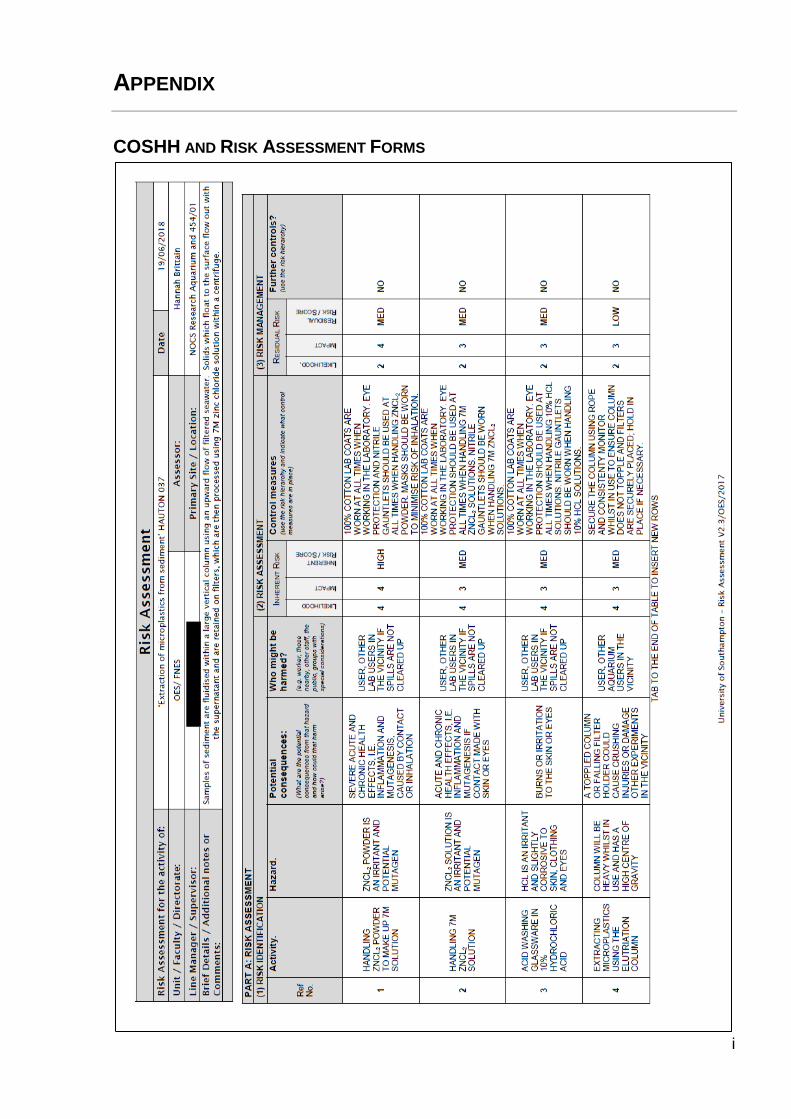
i
APPENDIX
COSHH AND RISK ASSESSMENT FORMS
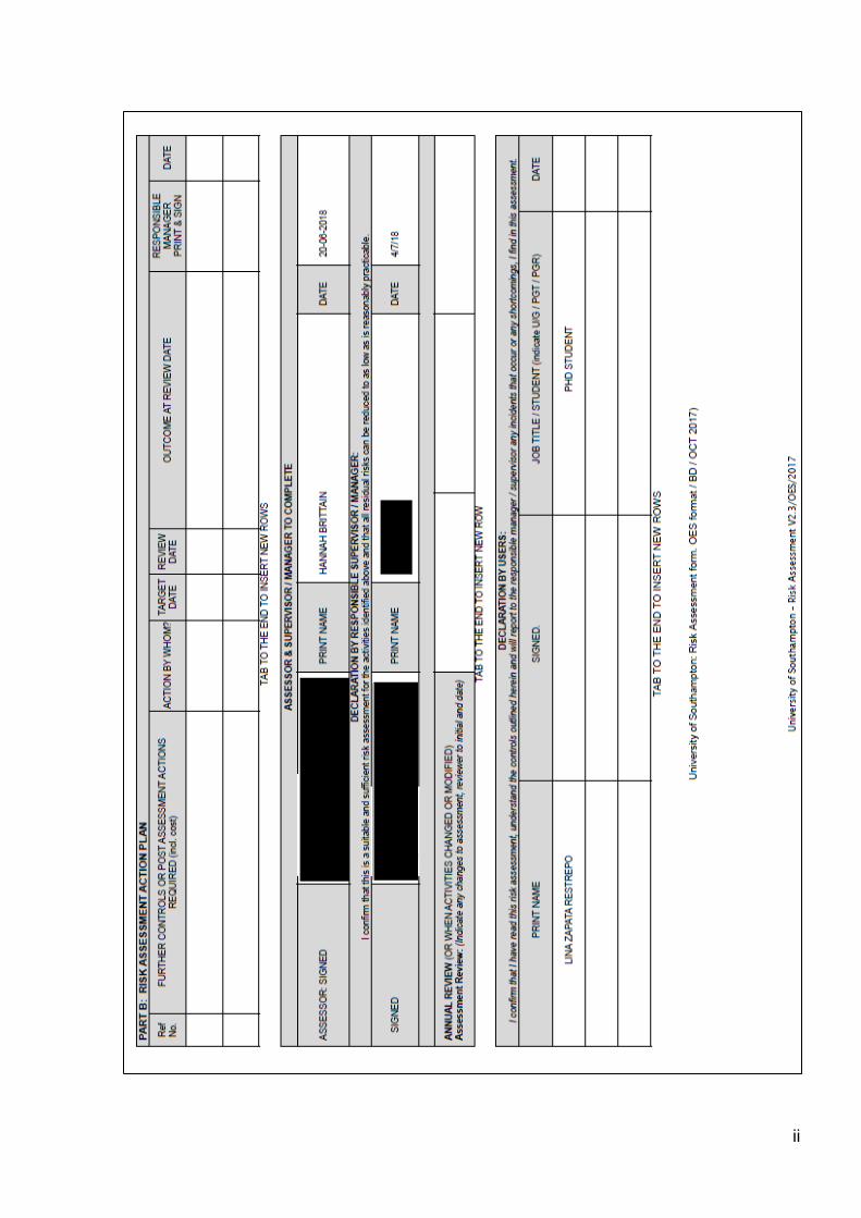
ii
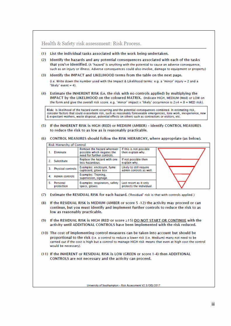
iii
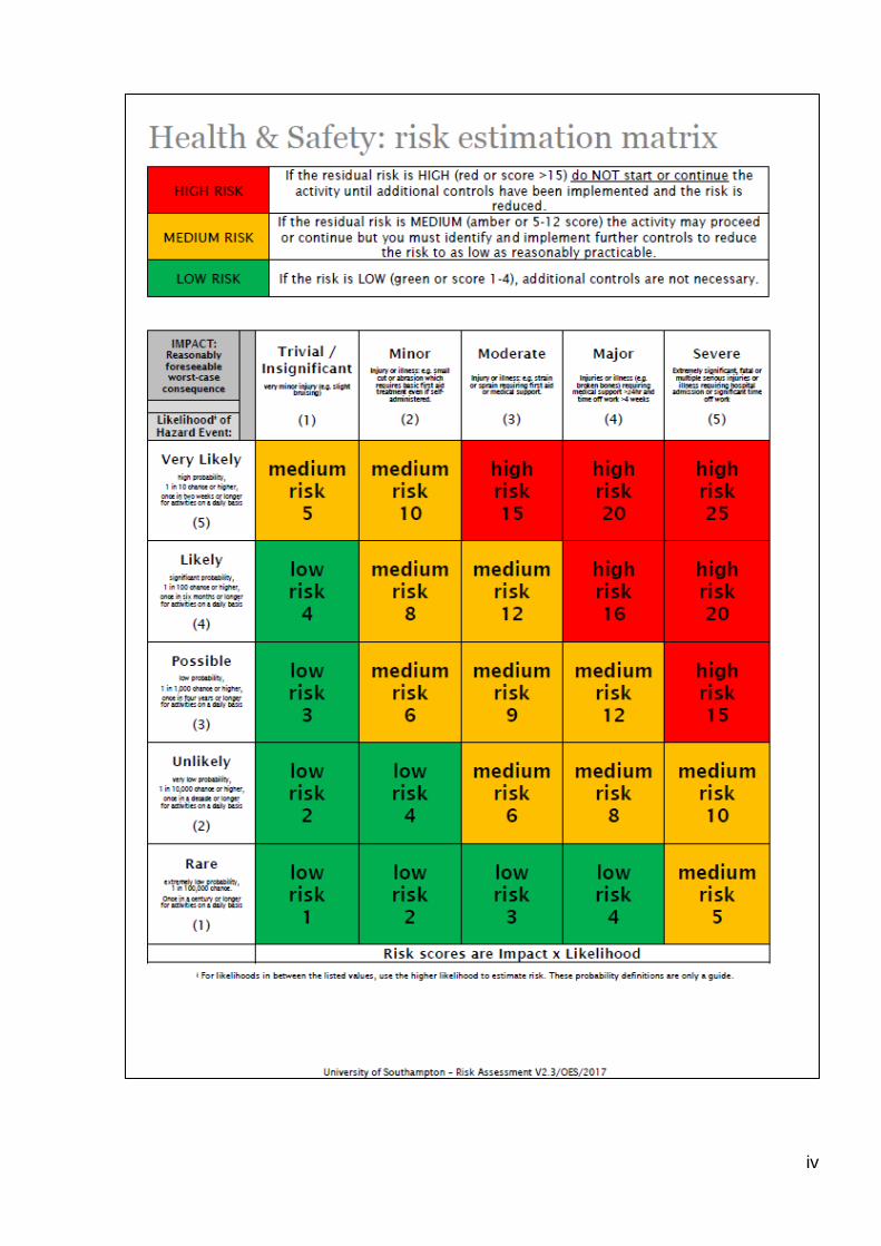
iv
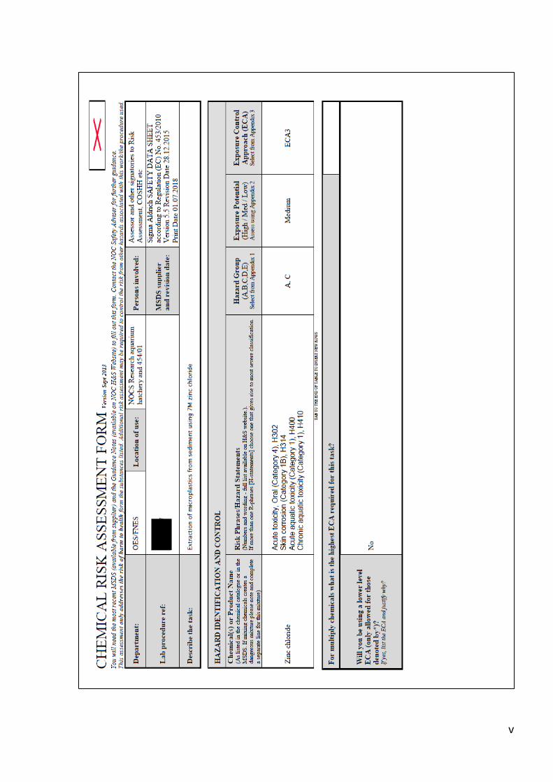
v
vi
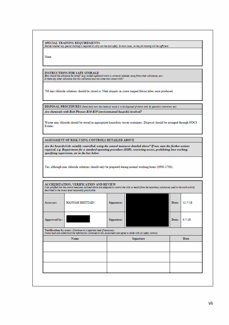
vii
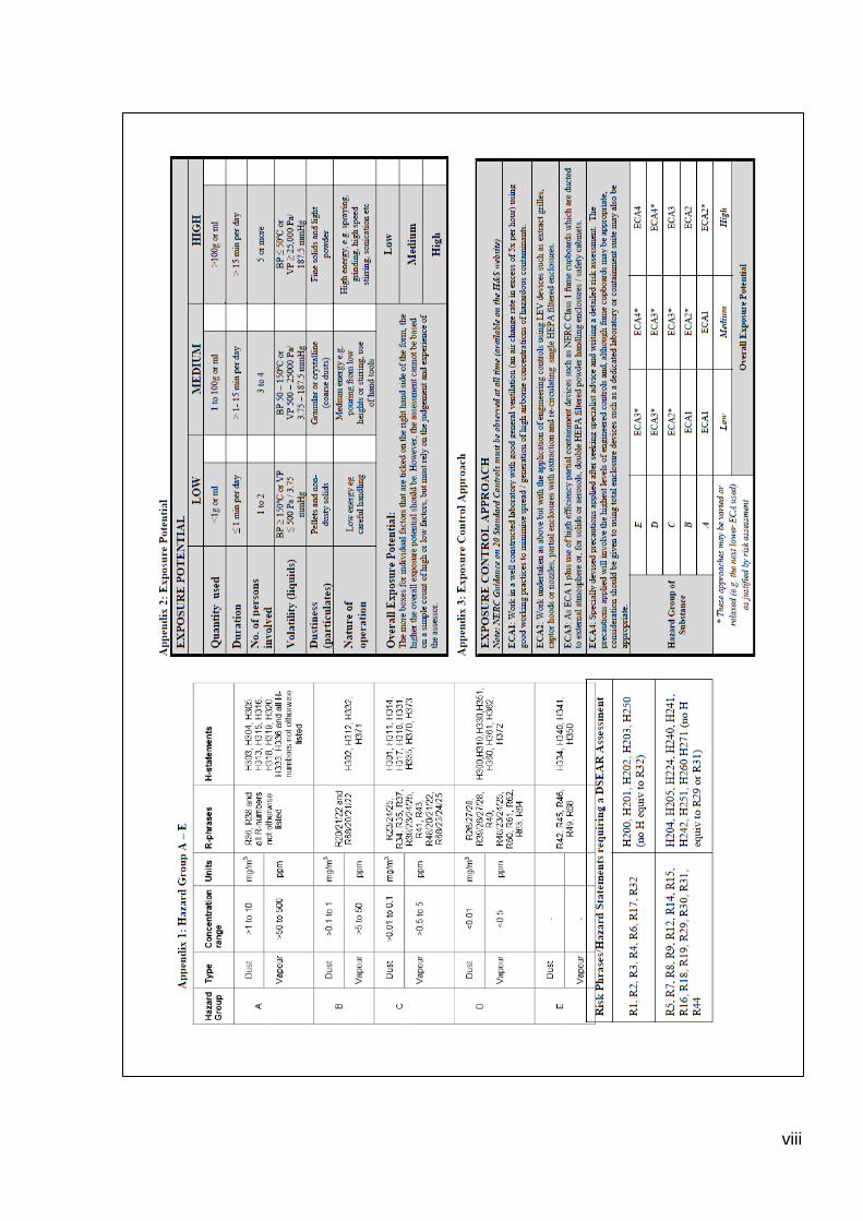
viii
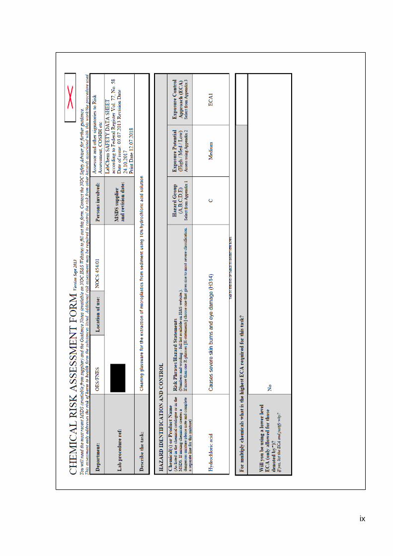
ix
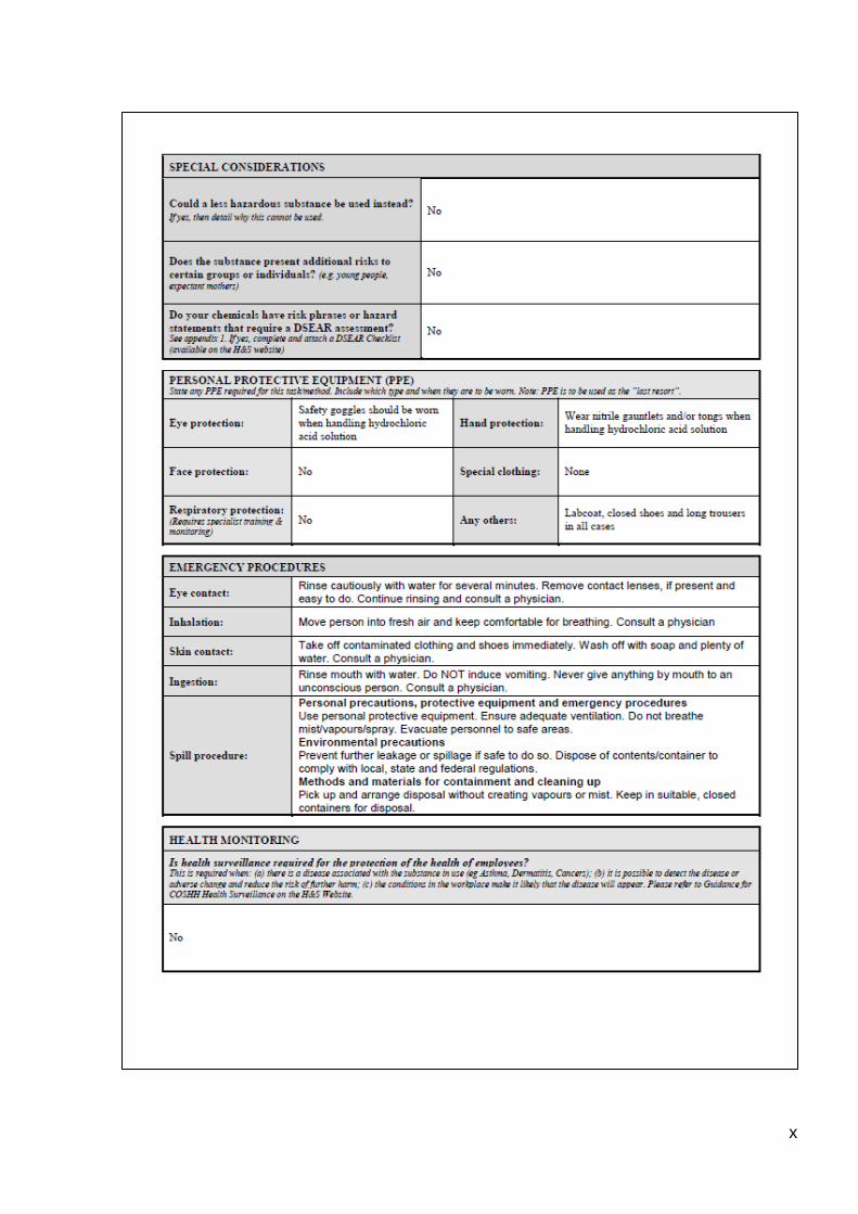
x
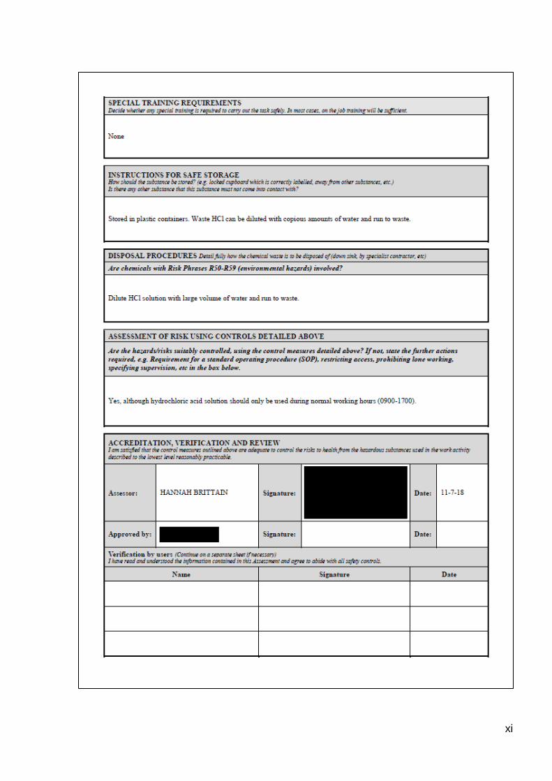
xi
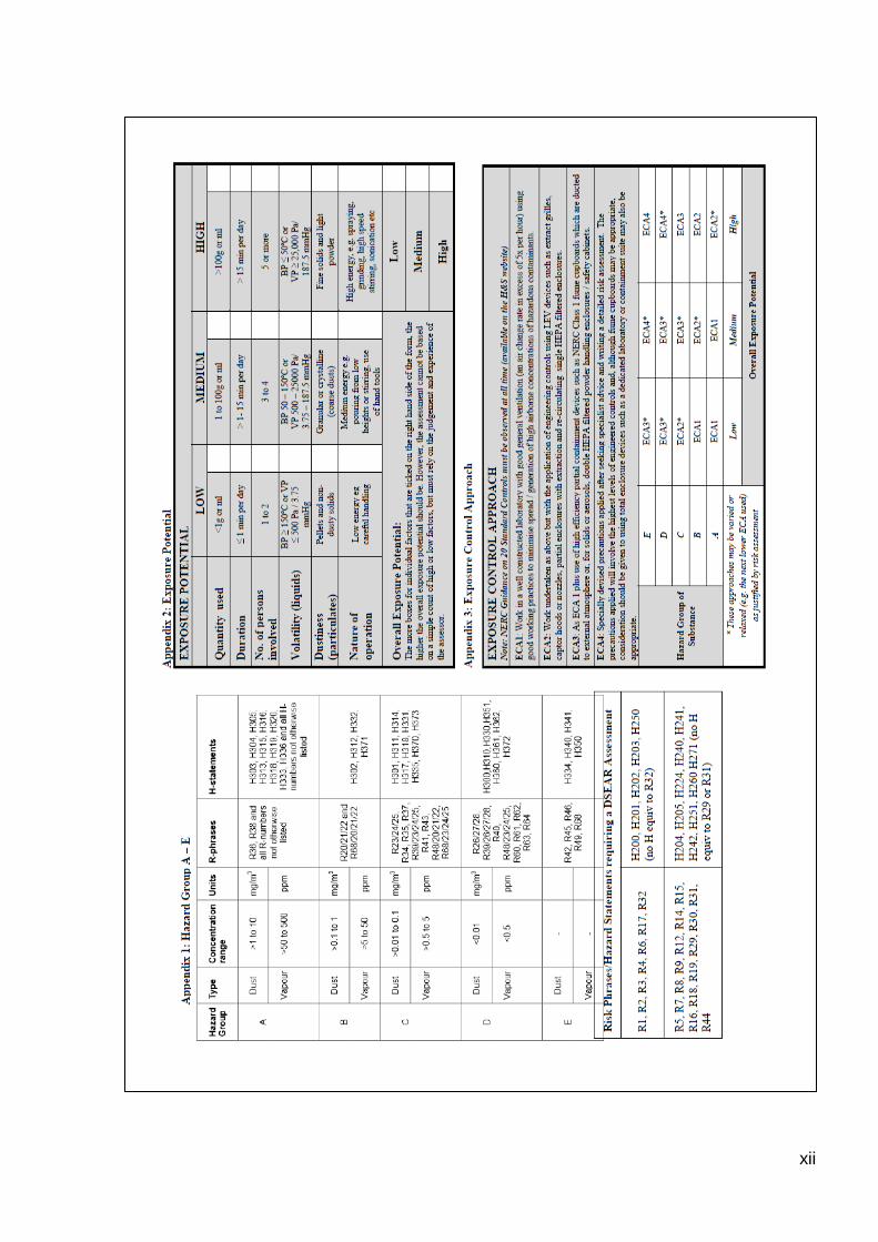
xii
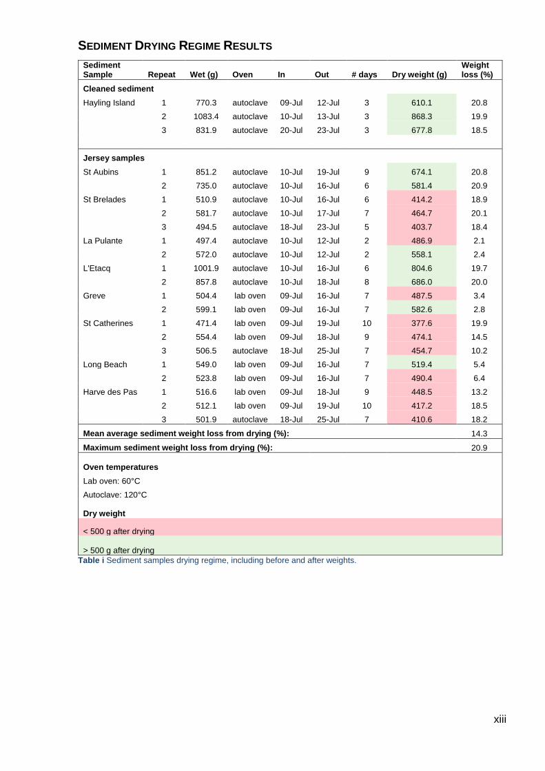
xiii
SEDIMENT DRYING REGIME RESULTS
Sediment Sample Repeat Wet (g) Oven In Out # days Dry weight (g)
Weight loss (%)
Cleaned sediment
Hayling Island 1 770.3 autoclave 09-Jul 12-Jul 3 610.1 20.8
2 1083.4 autoclave 10-Jul 13-Jul 3 868.3 19.9
3 831.9 autoclave 20-Jul 23-Jul 3 677.8 18.5
Jersey samples
St Aubins 1 851.2 autoclave 10-Jul 19-Jul 9 674.1 20.8
2 735.0 autoclave 10-Jul 16-Jul 6 581.4 20.9
St Brelades 1 510.9 autoclave 10-Jul 16-Jul 6 414.2 18.9
2 581.7 autoclave 10-Jul 17-Jul 7 464.7 20.1
3 494.5 autoclave 18-Jul 23-Jul 5 403.7 18.4
La Pulante 1 497.4 autoclave 10-Jul 12-Jul 2 486.9 2.1
2 572.0 autoclave 10-Jul 12-Jul 2 558.1 2.4
L'Etacq 1 1001.9 autoclave 10-Jul 16-Jul 6 804.6 19.7
2 857.8 autoclave 10-Jul 18-Jul 8 686.0 20.0
Greve 1 504.4 lab oven 09-Jul 16-Jul 7 487.5 3.4
2 599.1 lab oven 09-Jul 16-Jul 7 582.6 2.8
St Catherines 1 471.4 lab oven 09-Jul 19-Jul 10 377.6 19.9
2 554.4 lab oven 09-Jul 18-Jul 9 474.1 14.5
3 506.5 autoclave 18-Jul 25-Jul 7 454.7 10.2
Long Beach 1 549.0 lab oven 09-Jul 16-Jul 7 519.4 5.4
2 523.8 lab oven 09-Jul 16-Jul 7 490.4 6.4
Harve des Pas 1 516.6 lab oven 09-Jul 18-Jul 9 448.5 13.2
2 512.1 lab oven 09-Jul 19-Jul 10 417.2 18.5
3 501.9 autoclave 18-Jul 25-Jul 7 410.6 18.2
Mean average sediment weight loss from drying (%): 14.3
Maximum sediment weight loss from drying (%): 20.9
Oven temperatures
Lab oven: 60°C
Autoclave: 120°C Dry weight
< 500 g after drying
> 500 g after drying
Table i Sediment samples drying regime, including before and after weights.
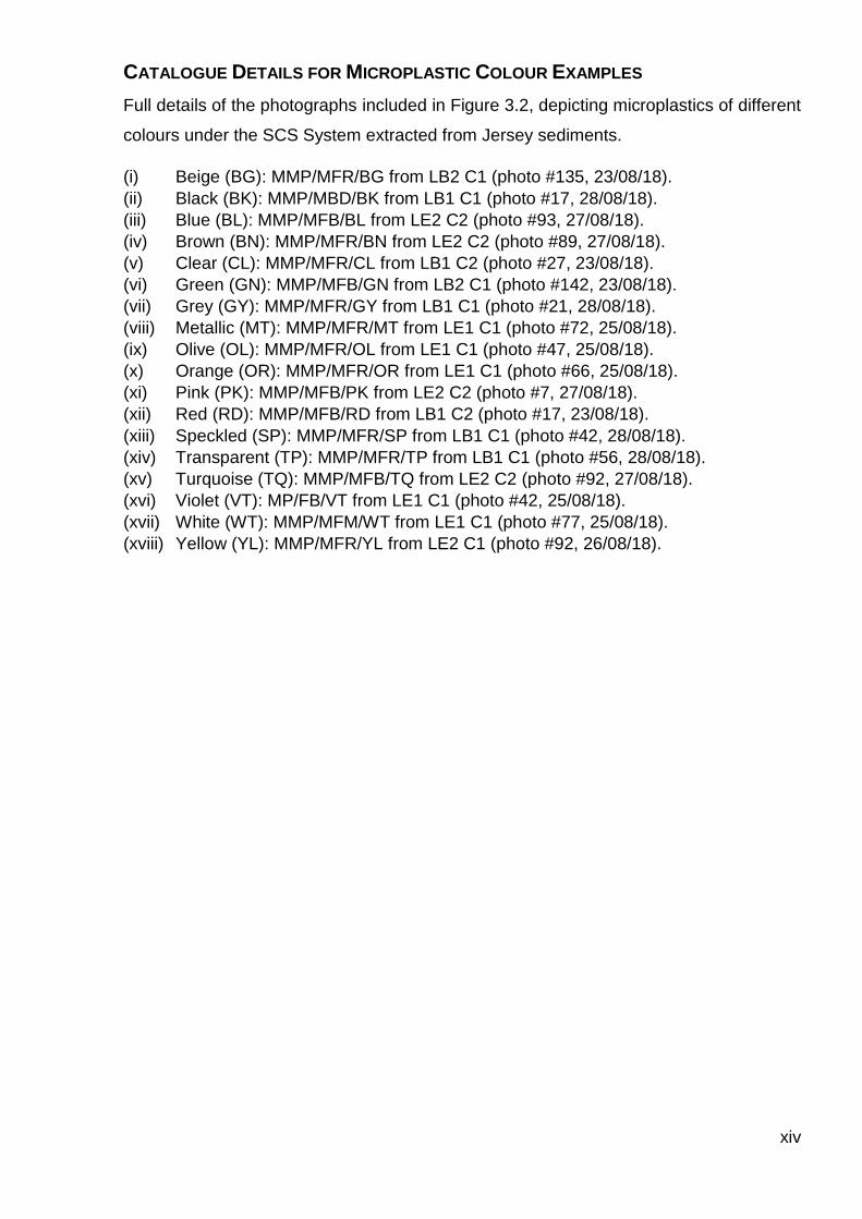
xiv
CATALOGUE DETAILS FOR MICROPLASTIC COLOUR EXAMPLES
Full details of the photographs included in Figure 3.2, depicting microplastics of different
colours under the SCS System extracted from Jersey sediments.
(i) Beige (BG): MMP/MFR/BG from LB2 C1 (photo #135, 23/08/18). (ii) Black (BK): MMP/MBD/BK from LB1 C1 (photo #17, 28/08/18). (iii) Blue (BL): MMP/MFB/BL from LE2 C2 (photo #93, 27/08/18). (iv) Brown (BN): MMP/MFR/BN from LE2 C2 (photo #89, 27/08/18). (v) Clear (CL): MMP/MFR/CL from LB1 C2 (photo #27, 23/08/18). (vi) Green (GN): MMP/MFB/GN from LB2 C1 (photo #142, 23/08/18). (vii) Grey (GY): MMP/MFR/GY from LB1 C1 (photo #21, 28/08/18). (viii) Metallic (MT): MMP/MFR/MT from LE1 C1 (photo #72, 25/08/18). (ix) Olive (OL): MMP/MFR/OL from LE1 C1 (photo #47, 25/08/18). (x) Orange (OR): MMP/MFR/OR from LE1 C1 (photo #66, 25/08/18). (xi) Pink (PK): MMP/MFB/PK from LE2 C2 (photo #7, 27/08/18). (xii) Red (RD): MMP/MFB/RD from LB1 C2 (photo #17, 23/08/18). (xiii) Speckled (SP): MMP/MFR/SP from LB1 C1 (photo #42, 28/08/18). (xiv) Transparent (TP): MMP/MFR/TP from LB1 C1 (photo #56, 28/08/18). (xv) Turquoise (TQ): MMP/MFB/TQ from LE2 C2 (photo #92, 27/08/18). (xvi) Violet (VT): MP/FB/VT from LE1 C1 (photo #42, 25/08/18). (xvii) White (WT): MMP/MFM/WT from LE1 C1 (photo #77, 25/08/18). (xviii) Yellow (YL): MMP/MFR/YL from LE2 C1 (photo #92, 26/08/18).
xv
GRAIN SIZE ANALYSIS DATA AND DISTRIBUTION GRAPHS
An explanation of how the grain size data was obtained through GRADISTAT Version 8.0
(Blott and Pye, 2001) using the above raw data is given below:
“The sample statistics are calculated using the Method of Moments in Microsoft Visual
Basic programming language: mean, mode(s), sorting (standard deviation), skewness,
kurtosis, D10, D50, D90, D90/D10, D90-D10, D75/D25 and D75-D25. Grain size parameters are
calculated arithmetically and geometrically (in microns – μm) and logarithmically (using
the phi scale – ϕ) (Krumbein and Pettijohn, 1938). Linear interpolation is also used to
calculate statistical parameters by the Folk and Ward (1957) graphical method and derive
physical descriptions (such as “very coarse sand” and “moderately sorted”). The program
also provides a physical description of the textural group which the sample belongs to
and the sediment name (such as “fine gravelly coarse sand”) after Folk (1954). Also
included is a table giving the percentage of grains falling into each size fraction, modified
from Udden (1914) and Wentworth (1922). In terms of graphical output, the program
provides graphs of the grain size distribution and cumulative distribution of the data in
both metric and phi units, and displays the sample grain size on triangular diagrams.”
(Blott and Pye, 2001).
Class Weight Retained (g) in Different Samples
Sample name: St Aubins 1 St Aubins 2 L'Etacq 1 L'Etacq 2 Long Beach 1 Long Beach 2 Spiked (PA) Spiked (PS) Spiked (PVC)
Initial Sample Weight (g): 500.00 500.00 500.00 500.00 500.00 500.00 500.00 500.00 500.00
Post-Analysis Sample Weight (g) 449.66 420.67 329.76 486.28 493.38 488.26 491.04 492.75 484.89
Aperture (μm)
38.00 8.24 6.17 0.00 0.00 0.01 0.00 0.23 0.28 0.29
63.00 71.85 60.27 0.04 0.03 0.06 0.07 1.37 1.98 1.79
90.00 348.04 336.87 3.38 4.03 8.32 12.53 42.60 45.36 45.07
125.00 19.34 15.56 86.98 105.18 52.38 66.50 165.67 153.42 174.58
180.00 1.76 1.42 225.17 354.93 143.43 145.65 223.19 239.54 208.73
250.00 0.35 0.25 12.59 19.32 126.10 108.74 22.70 21.40 20.88
355.00 0.07 0.07 1.30 2.21 83.36 61.70 6.60 5.90 5.99
500.00 0.01 0.03 0.29 0.44 59.87 56.42 5.07 4.65 4.70
710.00 0.00 0.01 0.01 0.08 14.73 22.98 3.78 3.37 3.53
1000.00 0.00 0.02 0.00 0.06 5.12 13.67 19.83 16.85 19.33
Table ii Grain size analysis raw data for all sediment samples
xvi
SIEVING ERROR: SAMPLE STATISTICS
SAMPLE IDENTITY: SA1 ANALYST & DATE: Hannah Brittain, 8/31/2018
SAMPLE TYPE: Unimodal, Very Well Sorted TEXTURAL GROUP: Sand
SEDIMENT NAME: Very Well Sorted Very Fine Sand
GRAIN SIZE DISTRIBUTION
MODE 1: GRAVEL: COARSE SAND: 0.0%
MODE 2: SAND: MEDIUM SAND: 0.1%
MODE 3: MUD: FINE SAND: 4.7%
D10: V FINE SAND: 93.4%
MEDIAN or D50: V COARSE GRAVEL: V COARSE SILT: 1.8%
D90: COARSE GRAVEL: COARSE SILT: 0.0%
(D90 / D10): MEDIUM GRAVEL: MEDIUM SILT: 0.0%
(D90 - D10): FINE GRAVEL: FINE SILT: 0.0%
(D75 / D25): V FINE GRAVEL: V FINE SILT: 0.0%
(D75 - D25): V COARSE SAND: CLAY: 0.0%
Logarithmic
f
MEAN : 3.309
SORTING (s): 0.272
SKEWNESS (Sk ): 0.745
KURTOSIS (K ): 8.278
2.417 -0.745 -0.240 0.240 Fine Skew ed
36.37 8.278 1.185 1.185 Leptokurtic
Very Fine Sand
19.61 1.207 1.189 0.250 Very Well Sorted
mm mm mm f
104.1 100.9 102.1 3.293
METHOD OF MOMENTS FOLK & WARD METHOD
Arithmetic Geometric Geometric Logarithmic Description
1.236 1.098 0.0%
21.94 0.306 0.0%
1.617 1.229 0.0%
46.67 0.694 0.0%
75.60 3.032
103.2 3.277 0.0%
122.3 3.725 0.0%
98.2%
1.8%
11.2%
mm f
107.5 3.237 0.0%
)(x
Figure i Grain size analysis data and distribution graph for SA1
xvii
SIEVING ERROR: SAMPLE STATISTICS
SAMPLE IDENTITY: SA2 ANALYST & DATE: Hannah Brittain, 8/31/2018
SAMPLE TYPE: Unimodal, Very Well Sorted TEXTURAL GROUP: Sand
SEDIMENT NAME: Very Well Sorted Very Fine Sand
GRAIN SIZE DISTRIBUTION
MODE 1: GRAVEL: COARSE SAND: 0.0%
MODE 2: SAND: MEDIUM SAND: 0.1%
MODE 3: MUD: FINE SAND: 4.0%
D10: V FINE SAND: 94.4%
MEDIAN or D50: V COARSE GRAVEL: V COARSE SILT: 1.4%
D90: COARSE GRAVEL: COARSE SILT: 0.0%
(D90 / D10): MEDIUM GRAVEL: MEDIUM SILT: 0.0%
(D90 - D10): FINE GRAVEL: FINE SILT: 0.0%
(D75 / D25): V FINE GRAVEL: V FINE SILT: 0.0%
(D75 - D25): V COARSE SAND: CLAY: 0.0%
Logarithmic
f
MEAN : 3.301
SORTING (s): 0.255
SKEWNESS (Sk ): 0.628
KURTOSIS (K ): 11.41
4.721 -1.519 -0.189 0.189 Fine Skew ed
120.1 30.76 1.186 1.186 Leptokurtic
Very Fine Sand
19.00 1.196 1.173 0.230 Very Well Sorted
mm mm mm f
104.5 101.5 103.6 3.271
METHOD OF MOMENTS FOLK & WARD METHOD
Arithmetic Geometric Geometric Logarithmic Description
1.228 1.095 0.0%
21.28 0.296 0.0%
1.566 1.213 0.0%
44.11 0.647 0.0%
77.91 3.035
103.6 3.271 0.0%
122.0 3.682 0.0%
98.6%
1.4%
18.9%
mm f
107.5 3.237 0.0%
)(x
Figure ii Grain size analysis data and distribution graph for SA2
xviii
SIEVING ERROR: SAMPLE STATISTICS
SAMPLE IDENTITY: LE1 ANALYST & DATE: Hannah Brittain, 8/31/2018
SAMPLE TYPE: Unimodal, Very Well Sorted TEXTURAL GROUP: Sand
SEDIMENT NAME: Very Well Sorted Fine Sand
GRAIN SIZE DISTRIBUTION
MODE 1: GRAVEL: COARSE SAND: 0.1%
MODE 2: SAND: MEDIUM SAND: 4.2%
MODE 3: MUD: FINE SAND: 94.7%
D10: V FINE SAND: 1.0%
MEDIAN or D50: V COARSE GRAVEL: V COARSE SILT: 0.0%
D90: COARSE GRAVEL: COARSE SILT: 0.0%
(D90 / D10): MEDIUM GRAVEL: MEDIUM SILT: 0.0%
(D90 - D10): FINE GRAVEL: FINE SILT: 0.0%
(D75 / D25): V FINE GRAVEL: V FINE SILT: 0.0%
(D75 - D25): V COARSE SAND: CLAY: 0.0%
Logarithmic
f
MEAN : 2.355
SORTING (s): 0.278
SKEWNESS (Sk ): 0.138
KURTOSIS (K ): 4.990
1.737 -0.138 -0.279 0.279 Fine Skew ed
17.75 4.990 0.992 0.992 Mesokurtic
Fine Sand
39.96 1.213 1.226 0.294 Very Well Sorted
mm mm mm f
201.9 195.4 193.9 2.367
METHOD OF MOMENTS FOLK & WARD METHOD
Arithmetic Geometric Geometric Logarithmic Description
1.300 1.177 0.0%
52.21 0.378 0.0%
1.719 1.383 0.0%
101.8 0.782 0.0%
141.5 2.040
200.7 2.317 0.0%
243.2 2.821 0.0%
100.0%
0.0%
51.6%
mm f
215.0 2.237 0.0%
)(x
Figure iii Grain size analysis data and distribution graph for LE1
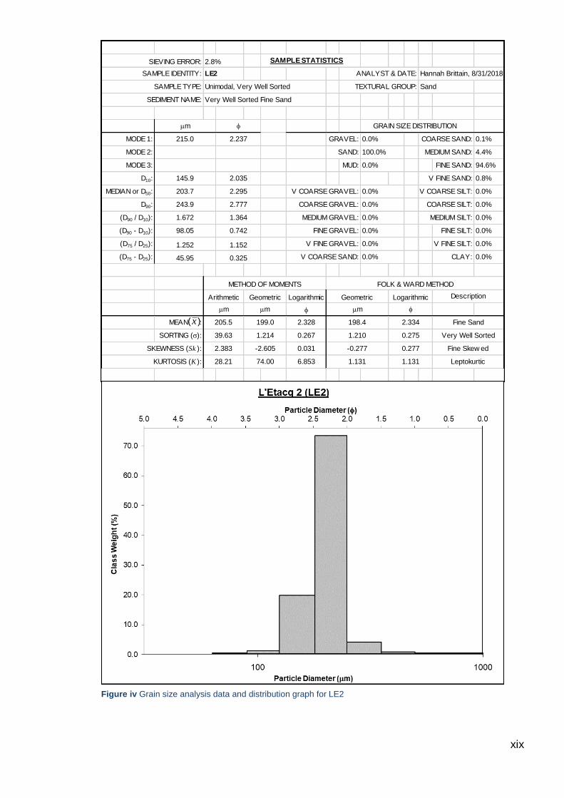
xix
SIEVING ERROR: SAMPLE STATISTICS
SAMPLE IDENTITY: LE2 ANALYST & DATE: Hannah Brittain, 8/31/2018
SAMPLE TYPE: Unimodal, Very Well Sorted TEXTURAL GROUP: Sand
SEDIMENT NAME: Very Well Sorted Fine Sand
GRAIN SIZE DISTRIBUTION
MODE 1: GRAVEL: COARSE SAND: 0.1%
MODE 2: SAND: MEDIUM SAND: 4.4%
MODE 3: MUD: FINE SAND: 94.6%
D10: V FINE SAND: 0.8%
MEDIAN or D50: V COARSE GRAVEL: V COARSE SILT: 0.0%
D90: COARSE GRAVEL: COARSE SILT: 0.0%
(D90 / D10): MEDIUM GRAVEL: MEDIUM SILT: 0.0%
(D90 - D10): FINE GRAVEL: FINE SILT: 0.0%
(D75 / D25): V FINE GRAVEL: V FINE SILT: 0.0%
(D75 - D25): V COARSE SAND: CLAY: 0.0%
Logarithmic
f
MEAN : 2.328
SORTING (s): 0.267
SKEWNESS (Sk ): 0.031
KURTOSIS (K ): 6.853
2.383 -2.605 -0.277 0.277 Fine Skew ed
28.21 74.00 1.131 1.131 Leptokurtic
Fine Sand
39.63 1.214 1.210 0.275 Very Well Sorted
mm mm mm f
205.5 199.0 198.4 2.334
METHOD OF MOMENTS FOLK & WARD METHOD
Arithmetic Geometric Geometric Logarithmic Description
1.252 1.152 0.0%
45.95 0.325 0.0%
1.672 1.364 0.0%
98.05 0.742 0.0%
145.9 2.035
203.7 2.295 0.0%
243.9 2.777 0.0%
100.0%
0.0%
2.8%
mm f
215.0 2.237 0.0%
)(x
Figure iv Grain size analysis data and distribution graph for LE2
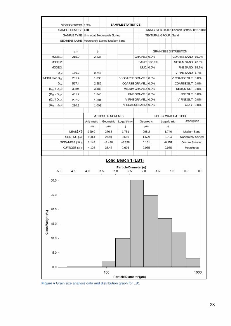
xx
SIEVING ERROR: SAMPLE STATISTICS
SAMPLE IDENTITY: LB1 ANALYST & DATE: Hannah Brittain, 8/31/2018
SAMPLE TYPE: Unimodal, Moderately Sorted TEXTURAL GROUP: Sand
SEDIMENT NAME: Moderately Sorted Medium Sand
GRAIN SIZE DISTRIBUTION
MODE 1: GRAVEL: COARSE SAND: 16.2%
MODE 2: SAND: MEDIUM SAND: 42.5%
MODE 3: MUD: FINE SAND: 39.7%
D10: V FINE SAND: 1.7%
MEDIAN or D50: V COARSE GRAVEL: V COARSE SILT: 0.0%
D90: COARSE GRAVEL: COARSE SILT: 0.0%
(D90 / D10): MEDIUM GRAVEL: MEDIUM SILT: 0.0%
(D90 - D10): FINE GRAVEL: FINE SILT: 0.0%
(D75 / D25): V FINE GRAVEL: V FINE SILT: 0.0%
(D75 - D25): V COARSE SAND: CLAY: 0.0%
Logarithmic
f
MEAN : 1.751
SORTING (s): 0.689
SKEWNESS (Sk ): -0.338
KURTOSIS (K ): 2.606
1.148 -4.438 0.151 -0.151 Coarse Skew ed
4.126 35.47 0.935 0.935 Mesokurtic
Medium Sand
168.4 2.091 1.629 0.704 Moderately Sorted
mm mm mm f
329.0 276.5 298.2 1.746
METHOD OF MOMENTS FOLK & WARD METHOD
Arithmetic Geometric Geometric Logarithmic Description
2.012 1.801 0.0%
210.2 1.009 0.0%
3.594 3.483 0.0%
431.2 1.845 0.0%
166.2 0.743
281.4 1.830 0.0%
597.4 2.589 0.0%
100.0%
0.0%
1.3%
mm f
215.0 2.237 0.0%
)(x
Figure v Grain size analysis data and distribution graph for LB1
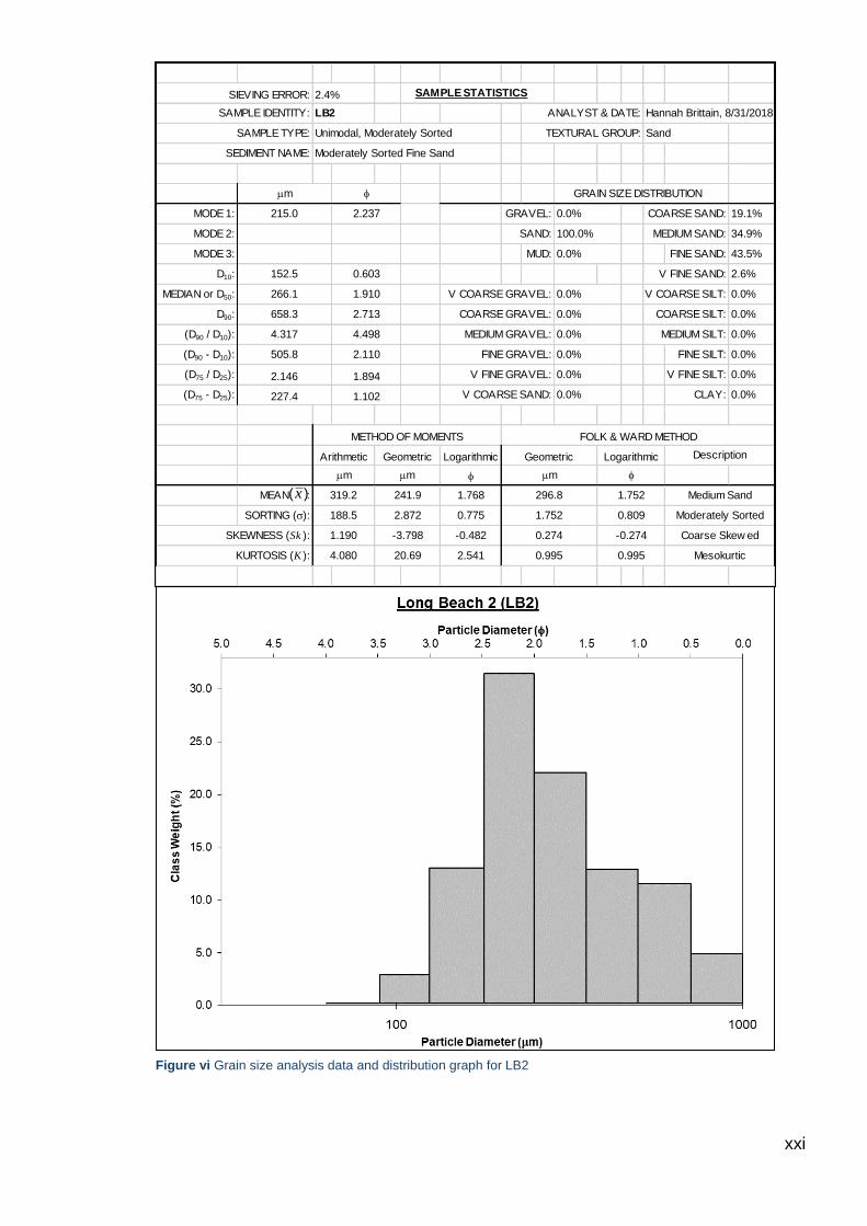
xxi
SIEVING ERROR: SAMPLE STATISTICS
SAMPLE IDENTITY: LB2 ANALYST & DATE: Hannah Brittain, 8/31/2018
SAMPLE TYPE: Unimodal, Moderately Sorted TEXTURAL GROUP: Sand
SEDIMENT NAME: Moderately Sorted Fine Sand
GRAIN SIZE DISTRIBUTION
MODE 1: GRAVEL: COARSE SAND: 19.1%
MODE 2: SAND: MEDIUM SAND: 34.9%
MODE 3: MUD: FINE SAND: 43.5%
D10: V FINE SAND: 2.6%
MEDIAN or D50: V COARSE GRAVEL: V COARSE SILT: 0.0%
D90: COARSE GRAVEL: COARSE SILT: 0.0%
(D90 / D10): MEDIUM GRAVEL: MEDIUM SILT: 0.0%
(D90 - D10): FINE GRAVEL: FINE SILT: 0.0%
(D75 / D25): V FINE GRAVEL: V FINE SILT: 0.0%
(D75 - D25): V COARSE SAND: CLAY: 0.0%
Logarithmic
f
MEAN : 1.768
SORTING (s): 0.775
SKEWNESS (Sk ): -0.482
KURTOSIS (K ): 2.541
1.190 -3.798 0.274 -0.274 Coarse Skew ed
4.080 20.69 0.995 0.995 Mesokurtic
Medium Sand
188.5 2.872 1.752 0.809 Moderately Sorted
mm mm mm f
319.2 241.9 296.8 1.752
METHOD OF MOMENTS FOLK & WARD METHOD
Arithmetic Geometric Geometric Logarithmic Description
2.146 1.894 0.0%
227.4 1.102 0.0%
4.317 4.498 0.0%
505.8 2.110 0.0%
152.5 0.603
266.1 1.910 0.0%
658.3 2.713 0.0%
100.0%
0.0%
2.4%
mm f
215.0 2.237 0.0%
)(x
Figure vi Grain size analysis data and distribution graph for LB2
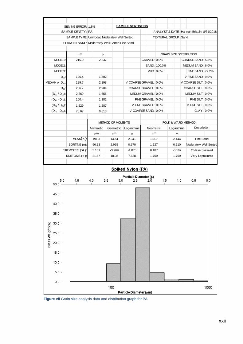
xxii
SIEVING ERROR: SAMPLE STATISTICS
SAMPLE IDENTITY: PA ANALYST & DATE: Hannah Brittain, 8/31/2018
SAMPLE TYPE: Unimodal, Moderately Well Sorted TEXTURAL GROUP: Sand
SEDIMENT NAME: Moderately Well Sorted Fine Sand
GRAIN SIZE DISTRIBUTION
MODE 1: GRAVEL: COARSE SAND: 5.8%
MODE 2: SAND: MEDIUM SAND: 6.0%
MODE 3: MUD: FINE SAND: 79.2%
D10: V FINE SAND: 9.0%
MEDIAN or D50: V COARSE GRAVEL: V COARSE SILT: 0.0%
D90: COARSE GRAVEL: COARSE SILT: 0.0%
(D90 / D10): MEDIUM GRAVEL: MEDIUM SILT: 0.0%
(D90 - D10): FINE GRAVEL: FINE SILT: 0.0%
(D75 / D25): V FINE GRAVEL: V FINE SILT: 0.0%
(D75 - D25): V COARSE SAND: CLAY: 0.0%
Logarithmic
f
MEAN : 2.341
SORTING (s): 0.670
SKEWNESS (Sk ): -1.875
KURTOSIS (K ): 7.628
3.161 -3.969 0.107 -0.107 Coarse Skew ed
21.67 18.98 1.759 1.759 Very Leptokurtic
Fine Sand
96.83 2.935 1.527 0.610 Moderately Well Sorted
mm mm mm f
191.3 149.4 183.7 2.444
METHOD OF MOMENTS FOLK & WARD METHOD
Arithmetic Geometric Geometric Logarithmic Description
1.529 1.287 0.0%
78.67 0.613 0.0%
2.269 1.656 0.0%
160.4 1.182 0.0%
126.4 1.802
189.7 2.398 0.0%
286.7 2.984 0.0%
100.0%
0.0%
1.8%
mm f
215.0 2.237 0.0%
)(x
Figure vii Grain size analysis data and distribution graph for PA
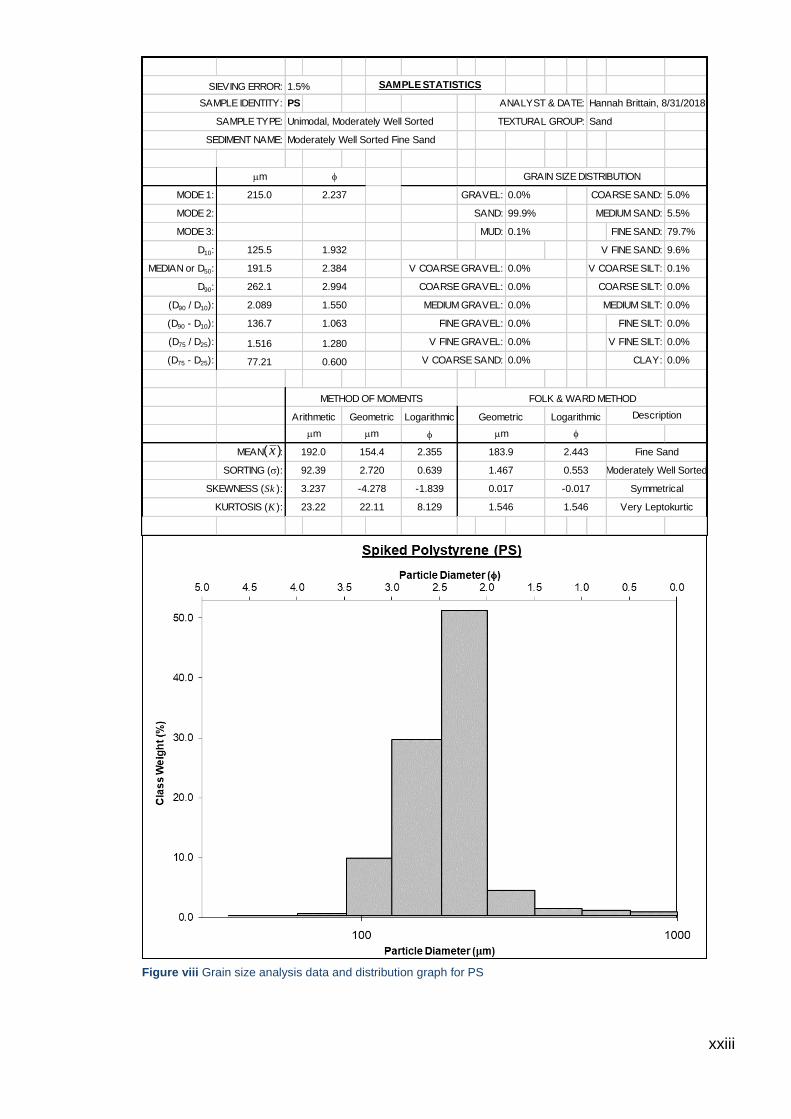
xxiii
SIEVING ERROR: SAMPLE STATISTICS
SAMPLE IDENTITY: PS ANALYST & DATE: Hannah Brittain, 8/31/2018
SAMPLE TYPE: Unimodal, Moderately Well Sorted TEXTURAL GROUP: Sand
SEDIMENT NAME: Moderately Well Sorted Fine Sand
GRAIN SIZE DISTRIBUTION
MODE 1: GRAVEL: COARSE SAND: 5.0%
MODE 2: SAND: MEDIUM SAND: 5.5%
MODE 3: MUD: FINE SAND: 79.7%
D10: V FINE SAND: 9.6%
MEDIAN or D50: V COARSE GRAVEL: V COARSE SILT: 0.1%
D90: COARSE GRAVEL: COARSE SILT: 0.0%
(D90 / D10): MEDIUM GRAVEL: MEDIUM SILT: 0.0%
(D90 - D10): FINE GRAVEL: FINE SILT: 0.0%
(D75 / D25): V FINE GRAVEL: V FINE SILT: 0.0%
(D75 - D25): V COARSE SAND: CLAY: 0.0%
Logarithmic
f
MEAN : 2.355
SORTING (s): 0.639
SKEWNESS (Sk ): -1.839
KURTOSIS (K ): 8.129
3.237 -4.278 0.017 -0.017 Symmetrical
23.22 22.11 1.546 1.546 Very Leptokurtic
Fine Sand
92.39 2.720 1.467 0.553 Moderately Well Sorted
mm mm mm f
192.0 154.4 183.9 2.443
METHOD OF MOMENTS FOLK & WARD METHOD
Arithmetic Geometric Geometric Logarithmic Description
1.516 1.280 0.0%
77.21 0.600 0.0%
2.089 1.550 0.0%
136.7 1.063 0.0%
125.5 1.932
191.5 2.384 0.0%
262.1 2.994 0.0%
99.9%
0.1%
1.5%
mm f
215.0 2.237 0.0%
)(x
Figure viii Grain size analysis data and distribution graph for PS
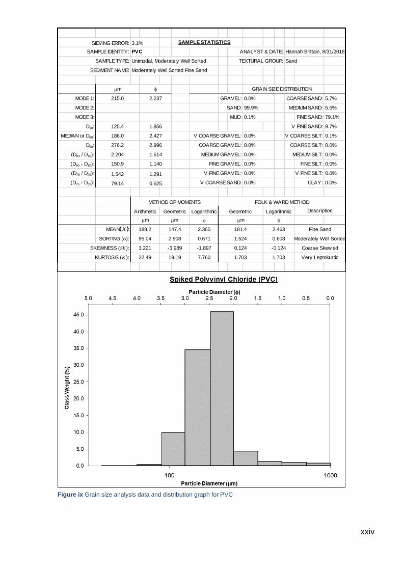
xxiv
SIEVING ERROR: SAMPLE STATISTICS
SAMPLE IDENTITY: PVC ANALYST & DATE: Hannah Brittain, 8/31/2018
SAMPLE TYPE: Unimodal, Moderately Well Sorted TEXTURAL GROUP: Sand
SEDIMENT NAME: Moderately Well Sorted Fine Sand
GRAIN SIZE DISTRIBUTION
MODE 1: GRAVEL: COARSE SAND: 5.7%
MODE 2: SAND: MEDIUM SAND: 5.5%
MODE 3: MUD: FINE SAND: 79.1%
D10: V FINE SAND: 9.7%
MEDIAN or D50: V COARSE GRAVEL: V COARSE SILT: 0.1%
D90: COARSE GRAVEL: COARSE SILT: 0.0%
(D90 / D10): MEDIUM GRAVEL: MEDIUM SILT: 0.0%
(D90 - D10): FINE GRAVEL: FINE SILT: 0.0%
(D75 / D25): V FINE GRAVEL: V FINE SILT: 0.0%
(D75 - D25): V COARSE SAND: CLAY: 0.0%
Logarithmic
f
MEAN : 2.365
SORTING (s): 0.671
SKEWNESS (Sk ): -1.897
KURTOSIS (K ): 7.760
3.221 -3.989 0.124 -0.124 Coarse Skew ed
22.49 19.19 1.703 1.703 Very Leptokurtic
Fine Sand
95.04 2.908 1.524 0.608 Moderately Well Sorted
mm mm mm f
188.2 147.4 181.4 2.463
METHOD OF MOMENTS FOLK & WARD METHOD
Arithmetic Geometric Geometric Logarithmic Description
1.542 1.291 0.0%
79.14 0.625 0.0%
2.204 1.614 0.0%
150.9 1.140 0.0%
125.4 1.856
186.0 2.427 0.0%
276.2 2.996 0.0%
99.9%
0.1%
3.1%
mm f
215.0 2.237 0.0%
)(x
Figure ix Grain size analysis data and distribution graph for PVC