Optimality and Nonoptimality of the Base-stock Policyin Inventory Problems with Multiple Delivery Modes

Qi FengSchool of Management, the University of Texas at Dallas

Richardson, TX 75083-0688, USA

Guillermo GallegoDept. of Industrial Engineering and Operations Research

The Columbia University in the City of New York, USA

Suresh P. SethiSchool of Management, the University of Texas at Dallas

Richardson, TX 75083-0688, USA

Houmin YanSchool of Management, the University of Texas at Dallas

Richardson, TX 75083-0688, USA

andHanqin Zhang

Institute of Applied Mathematics

Academy of Mathematics and Systems Sciences

Academia Sinica, Beijing, 100080, China

February 1, 2004

We present a periodic review inventory model with multiple delivery modes and demandforecast updates. We generalize the notion of the base-stock policy for inventory systemwith multiple delivery modes. While base-stock policies are optimal for one or two consec-utive delivery modes, it is not so otherwise. For multiple consecutive delivery modes, weshow that only the fastest two modes have optimal base stocks, and provide simple counterexamples to show that the remaining ones do not. We investigate why the base-stock policyis or is not optimal in different situations.

Subject Classifications : Inventory, base-stock policies, multiple delivery modes.

1. Introduction

It is common in practice that a buyer chooses among different alternatives to replenish

his inventory for certain goods. Typically, the shorter is the lead time, the higher is the

procurement cost. Thus, the buyer may begin with ordering early with long lead times to save

1

money. As demand information unfolds gradually over time, the buyer is able to place several

more expensive orders to supplement the earlier order. The strategic importance of having

faster delivery options is underscored by the case of the fashion industry, in which many firms

have moved their major manufacturing facilities to Asian countries to take advantage of lower

production costs there. However, it takes weeks for container ships to reach North America.

When it is close to the selling season and new information indicates a demand surge, it

may then not be feasible for the firm to replenish its inventory through overseas orders and

still meet the increased demand. For this reason, many fashion industry firms still maintain

some of their domestic factories which, while producing goods at higher cost, can respond

quickly to demand surges. An important factor contributing to the higher cost of fast delivery

options is the transportation cost. An emergency order might be filled by air shipment, which

is certainly faster and more costly than the slower rail or maritime shipments. Moreover,

sourcing from multiple suppliers may also reduce the buyers’ procurement risks. It is quite

usual that different suppliers are characterized by different prices and lead times for the same

product. Suppliers who are capable of delivering faster may reasonably ask for higher prices.

In most of the studies on inventory models with replenishment lead time options, it is

assumed that there are two consecutive procurement modes available. That is, the lead times

of the two modes vary by exactly one period. This assumption is very restrictive. Under

many circumstances, there are more than two supply modes (Zhang 1996), and/or the modes

are not consecutive (Beyer and Ward 2000). To explore the general problem, we consider

N consecutive delivery modes. In the case of non-consecutive delivery modes, it is easy to

insert fictitious delivery modes as suggested in Sethi et al. (2001) to transform the problem

into one with consecutive modes. All one needs to do is to set the cost for any fictitious

mode to equal that for the next faster mode that is real. It should be clear that setting costs

in this way would mean that we can consider policies which do not issue orders using any of

the fictitious modes. Also, the case of N modes with lead times L+1, L+2, ..., L+N can be

reduced to our case by the standard device used in converting a single mode problem with a

lead time to one with no lead time. Thus, our N -consecutive-mode formulation enables us to

treat cases where fast and slow modes could be several orders of magnitude apart. A typical

case is that of deliveries by air and surface shipments. A real-life instance of such a case is

reported in an HP study by Beyer and Ward (2000). It concerns an important component

of HP Windows NT network server – MOD0 box. The MOD0 box is pre-assembled in

Singapore and then shipped to distribution centers, where the servers are finally assembled

2

and configured according to re-sellers’ specifications. The factory in Singapore can ship to

distribution centers in France, Canada and Mexico by either air or ocean. Suppose that the

air and sea mode lead times for a given distribution center are Ta and Ts, respectively. Then

we can add (Ts − Ta − 1) fictitious delivery modes between air and sea shipments to solve

the replenishment problem faced by the distribution center.

In this paper, we provide a general formulation of a finite-horizon periodic review inven-

tory system with multiple delivery modes. In each period, the decision maker can place N

types of orders. A type j order is characterized by its unit ordering cost and a lead time of

j periods. In the case of single delivery mode, it is well known that the optimal ordering

policy is a base-stock policy. A fundamental characteristic of the base-stock level in the

classical single delivery mode inventory problem is that the level is independent of the pre-

order inventory position, since any ordering policy can be converted to an order-up-to policy

simply by adding the order quantity to the inventory position. In the case of two consecutive

modes, it has also been shown that the optimal policy is of base stock type. When we move

to more than two modes, the issues become substantially more complicated because there

are N different inventory positions to consider in each period. How do we define base-stock

policies in this case? When is a base-stock policy optimal? We try to address these questions

in this paper.

The remainder of the paper is organized as follows. The next section briefly reviews the

related literature. In Section 3, we establish the model and discuss the condition under which

certain modes are not used. In Section 4, we summarize the discussion in the literature on

inventory models with single mode and two modes, and propose two different definitions

of the base-stock policies. Section 5 presents an example which shows that the optimal

ordering policy in inventory models with two non-consecutive modes is not a base-stock

policy in general. In Section 6, we discuss the policy structure of inventory models with

more than two modes. Finally, we conclude the paper in Section 7.

2. Literature Review

Since the early 50’s, papers by Arrow, Harris and Marschak (1951) and Dvoretzhy, Kiefer

and Wolfowitz (1952a,1952b) have stimulated a great deal of research on dynamic inventory

models. Since the space does not permit us to summarize the enormous inventory literature

that has accumulated over the last fifty years, we limit ourselves to giving an overview of

3

the related work on base-stock policies with particular emphasis on single product inventory

systems with multiple procurement modes.

2.1 Base-stock policies in problems with single delivery mode

The early discussions on the base-stock policy for systems involving a single product and

a single delivery mode have focused on proving its optimality under the situation that the

demands are independent. Examples can be found in Gaver (1959, 1961), Karlin (1958),

Karlin and Scarf (1958), etc. Bellman et al. (1955) and Karlin (1960) are the classical

papers for the stationary and nonstationary demand cases, respectively. Optimality of a

base-stock policy has been established in these situations.

Iglehart and Karlin (1962) first address the problem with dependent demand. They

consider an inventory model with the demand process governed by a discrete-time Markov

chain. In each period, the current value of the state of the chain decides the demand density

for that period. They first propose a “state-dependent” base-stock policy for a model with

linear ordering cost. Song and Zipkin (1997) and Sethi and Cheng (1997) show optimality of

a state-dependent base-stock policy to be optimal when the demand is modeled as a Markov-

modulated process, and when the fixed setup cost in their models is zero. Cheng and Sethi

(1999) extend the result of Markov-modulated demand models by introducing promotional

decisions.

Another stream of related research focuses on a product with multi-class demands pio-

neered by Veinott (1965a). Topkis (1968) considers an extended model with one replenish-

ment opportunity at the beginning of the horizon, convex holding cost in each period, and n

classes of demands each with a different penalty cost. He shows that a rationing level policy

is optimal. Under such a policy, one tries to satisfy demands with higher penalty costs first.

Moreover, the optimal post-action inventory position for each demand class is determined

by satisfying as much demand for that class as possible with existing stock, without letting

the inventory position drop below a certain critical number associated with that class. The

rationing level policy shares certain similarities with base-stock policies. The only difference

is that in Topkis’s model, the order is placed only at the beginning of the horizon, and the

demand is filled in each period with on-hand inventory. Thus, the direction of inventory

position change after an action is different from a usual ordering system. We shall point

out that the approach used in models with multi-class demands cannot be adopted to study

models with multiple delivery modes, since the structures of the cost functions are different.

4

Also there are discussions on base-stock policies for multi-product inventory systems (e.g.

Veinott 1965b,1970). Again, the problem structure is different from the one considered here.

2.2 Inventory models with two consecutive modes

The earliest discussion on inventory models with two delivery modes can be traced back

to Barankin (1961), who studies a single period problem. Daniel (1963) analyzes a multi-

period model with one regular order and one emergency order. Fukuda (1964) uses dynamic

programming approach to derive the optimal ordering policy for inventory models with two

delivery modes. Parallel to Fukuda, Neuts (1964) also proves the structure of the optimal

policy for a similar model. Veinott (1966) gives an alternative proof of Fukuda’s result

in a survey paper, where he applies an observation by Karush (1957). Recently, several

authors have studied different variations of the problem. As examples, we mention three

such studies. Sethi et al. (2001) introduce an information updating scheme into the model.

Lawson and Porteus (2000) address policy structure of a multi-echelon system with an option

of expediting at each location. Muharremoglu and Tsitsiklis (2003) extend the model of

Lawson and Porteus (2000) by allowing for expediting from any stage in the supply chain

to any downstream stage. Under a supermodularity assumption on the ordering costs, they

show the optimality of an extended echelon base-stock policy. However, the assumption

breaks down when converting a single-echelon, multi-mode inventory model with other than

two consecutive delivery modes. Thus, these studies show that in the case of two consecutive

delivery modes, a base-stock policy or a modified base-stock policy is optimal. That is, there

are two critical numbers, independent of the initial inventory position, such that the optimal

ordering policy is to order up to the critical numbers. As we will see in Section 4.2, the

critical number for the slower order is not unique. Depending on how this critical number is

chosen, the meaning of the base-stock level is different.

Aside from the discussions on policy structure, computational studies for inventory mod-

els with two modes also appear in the literature. For example, Moinzadeh and Nahmias

(1988) study a continuous-review inventory system, and Tagaras and Vlachos (2001) show

cost reduction by introducing a second replenishment option.

2.3 Inventory models with more than two modes

An inventory model with three consecutive delivery modes is first examined by Fukuda

(1964). He considers a special case when orders are placed only every other period. Under

5

this assumption, a base-stock policy is shown to be optimal. Implicitly, he shows that the

optimal order-up-to levels are independent of the initial inventory position. Zhang (1996)

extends Fukuda’s model by allowing three consecutive modes ordered every period. While

she claims the optimality of a base-stock policy under certain conditions, her claim is untrue

because of the errors in Lemma 1 and 2 in her paper. Feng et al. (2003) study an inventory

model with three consecutive delivery modes and demand forecast updates. They show that

there exist optimal base-stock levels for the two faster modes.

3. Problem Formulation and Effective Modes

In this section, we present our basic model and discuss the conditions under which some of

the delivery mode are never used in the ordering system.

3.1 Problem Formulation

We consider a finite horizon periodic review inventory system with N delivery modes. An

order via the ith delivery mode, i = 1, 2, ..., N , is an order associated with a lead time of i

periods, and is termed the type i order. The notation is summarized as follows:

〈1, T 〉 = 1, 2, ..., T, the time periods;

(Ω,F , P ) = the probability space;

Qik = the order quantity of type i order in period k, 1 6 k 6 T, 1 6 i 6 N ;

cik = the unit procurement cost of type i order in period k, 1 6 k 6 T, 1 6 i 6 N ;

Dk = the random demand in period k, 1 6 k 6 T ;

Rik = the ith determinant of demand in period k, 1 6 k 6 T, 1 6 i 6 N ;

xk = the inventory/backlog level at the beginning of period k, 1 6 k 6 T ;

yk = the initial inventory position at the beginning of period k, 1 6 k 6 T ;

zik = the post-order inventory position for period k + i − 1 viewed at the beginning

of period k,1 6 k 6 T, 1 6 i 6 N ;

Hk(·) = the inventory holding cost (assuming convex) in period k, 1 6 k 6 T ;

HT+1(·) = the inventory and/or penalty costs for the ending inventory/backlog.

Fig. 1 shows the inventory positions viewed at the beginning of period k (We denote

qiℓ as the realized value of Qi

ℓ). There are N inventory positions to consider, each of which

6

corresponds to one type of order. First, we review the initial inventory position yk, including

the inventory/backlog level xk and in-transit orders to be delivered at the end of period

k. The post-order inventory position in period k is simply the sum of yk and Q1k. Then

we examine the post-order inventory for the subsequent N − 1 periods. We observe that

in-transit orders qik+j−i

Ni=j+1 to be delivered in period k + j − 1 affect the ordering decision

only through their sum pjk. The post-order inventory position zj

k for period k+j−1 contains

all previous and current orders to be delivered by that time. Hence, we have the relation

zjk = zj−1

k + pjk + Qj

k.

Figure 1: Post-order inventory positions viewed at the beginning of period k.

q2k−1

q3k−2

Q1k

q4k−3

q5k−4

Q2k

q3k−1

q4k−2

q5k−3

... ...qN−1k−N+3

qNk−N+2

qN−1k−N+2

qNk−N+1

Q3k

q4k−1

q5k−2

... ...qN−1k−N+4

qNk−N+3

QN−1k

qNk−1 QN

k

......

...

-Period ℓ

z1k z2

k z3k zN−1

k zNk

= p1k = p2

k = p3k = pN−1

k

In-transit ordersto be deliveredin period ℓ

? ? ? ? ?

Post-orderinventory positionin period ℓ :

k k + 1 k + 2 k + N − 2 k + N − 1

Order placedin period kto be deliveredin period ℓ :

History of ordersto be deliveredin period ℓ :

... ...

-yk

We use the demand forecast updating scheme introduced in Sethi et al. (2001). Accord-

ingly, the demand Dk is hidden in the core of an N -layered onion containing uncertainties

modeled by random variables R1k, ..., R

Nk , Rk. The demand signal Rj

k is observed at the

beginning of period (k−N + j). At the end of period k, the last determinant Rk is observed

and demand is realized. Thus, the demand can be written as a function of the random

variables R1k, ..., R

Nk , Rk, i.e.,

Dk = dk(R1k, ..., R

Nk , Rk). (1)

For convenience in exposition, we assume that R1k, ..., R

Nk , Rk are independent random vari-

ables. We also define a set of variables called relevant demand history at the beginning of

7

period k as follows

Rk =

R1k, R2

k . . . . . . RNk ,

R1k+1, R2

k+1 . . . RN−1k+1 ,

... ..

... ..R1

k+N−1

.

At the beginning of period k, the values of Rjℓ

Nj=1, Rℓ

k−1ℓ=1 ∪ Rk are known. However, the

signals for the realized demands in the first (k − 1) periods are irrelevant for the ordering

decisions (Q1k, ..., Q

Nk ). Only the information Rk about future demands is relevant.

In this setting, R1k, ..., R

Nk , Rk16k6T capture completely the randomness of the under-

lying process. Let Fk16k6N be the filtration of the underline process. Then we can take

Fk as the sigma algebra generated by Rjℓ

Nj=1, Rℓ

k−1ℓ=1 ∪ Rk. We denote the corresponding

lower case rjk to be the observed value of the signal Rj

k. Explicitly, if we evaluate Dk at

period ℓ, then

Dk =

dk(R1k, ..., R

Nk , Rk), for ℓ 6 k − N,

dk(r1k, ..., r

ℓ−k+N−1k , Rℓ−k+N

k , ..., RNk , Rk), for k − N < ℓ 6 k,

dk(r1k, ..., r

Nk , rk), for ℓ > k + 1.

(2)

Remark 1 In reality, the demand forecast may not necessarily update exactly N + 1 times.

For example, in some period j ( k − N < j 6 k) there is no update for Dk, or information

for Dk may be acquired before period k−N +1. In the first case, we can simply set RN−(k−j)k

to any constant. In the second case, we can take R1k to contain all the information about Dk

gathered before the beginning period k − N + 1, since the first time we can order for period

k is at the beginning of period k − N + 1 when R1k is realized. Note that the conditional

distribution of R1k given Fj is different for different j > k − N + 1, which affects ordering

decisions before period k − N + 1. We take N + 1 forecast updates here just for the purpose

of exposition.

Now we can write the dynamic programming equation as follows:

Uk(xk, p1k, ..., p

N−1k ; rk) (3)

= Hk(xk) + minQ1

k>0,...,QNk >0

N∑

i=1

cikQ

ik +

E[

Uk+1

(

Ψ(Q1k); p

2k + Q2

k, ...., pN−1k + QN−1

k , QNk ; RN

k+1, . . . , R1K+N , r′k

)]

,

k = 1, 2, ..., T,

8

where

Ψ(Q1k) = xk + p1

k + Q1k − dk(r

1k, ..., r

Nk , Rk),

and r′k = rk − r1k, . . . , r

Nk .

In terms of inventory positions (z1k, ..., z

Nk ), (3) is equivalent to

Wk(yk, p2k, .., p

N−1k ; rk) = Uk(xk, p

1k, ..., p

N−1k , rk) − EHk(xk) (4)

= minz1k>yk,

zjk>zj−1+p

jk

c1k(z

1k − yk) +

N∑

j=2

cjk(z

jk − zj−1

k − pjk) + EHk+1(z

1k − Dk)

+EWk+1

(

z2k − Dk, z

3k − z2

k, ..., zNk − zN−1

k ; RNk+1, . . . , R

1K+N , r′k

)

.

Throughout this paper, we denote Jk(z1k, ..., z

Nk ; rk) or Jk(Q

1k, ..., Q

Nk ; rk) to be the objec-

tive function for period k, i.e., the function inside “min” of (3) or (4). Also, (z1k, ..., z

Nk ) is the

unconstrained minimizer to Jk, (z1∗k , ..., zN∗

k ) are the optimal post-order inventory positions,

(Q1∗k , ..., QN∗

k ) are the optimal order quantities, and zik is the optimal base-stock level for the

type i order (if exists).

3.2 Ordering Costs and Effective Modes

In reality, some of the delivery modes in certain period may never be used. In what follows,

we identify conditions under which certain modes are never ordered.

Proposition 1 If cjk > cj−i

k+i for some j > 1 and 1 6 i < j, then there is an optimal solution

with no type j order placed in period k. That is, Qj∗k = 0 or zj∗

k = zj−1∗k + pj

k.

Proof. Without loss of generality we set i = 1. Suppose the optimal solution in period

k is (Q1∗k , ..., QN∗

k ) with Qj∗k > 0. Then,

Jk(Q1∗k , ..., QN∗

k ; rk)

=N

∑

i=1

cikQ

i∗k + EHk+1(xk + ΣN

i=2qik−i+1 + Q1∗

k − Dk)

+EUk+1

(

Ψ(Q1∗k ); p2

k + Q2∗k , ..., pN−1

k + QN−1∗k , QN∗

k ; Rk+1

)

=N

∑

i=1

cikQ

i∗k + EHk+1(xk + ΣN

i=2qik−i+1 + Q1∗

k − Dk)

9

+E minQi

k+1>0,

i=1,...,N

[

N∑

i=1

cik+1Q

ik+1 (5)

+EUk+2

(

Ψ(Q1k+1); p

3k + Q3∗

k + Q2k+1, ..., p

N−1k + QN−1∗

k + QN−2k+1 , QN∗

k + QN−1k+1 , QN

k+1; Rk+2

)]

>∑

i6=j

cikQ

i∗k + EHk+1(xk + ΣN

i=2qik−i+1 + Q1∗

k − Dk)

+E minQi

k+1>0,

i=1,...j−2,j...,N,

Qj−1k+1+Q

j∗k >0

[

∑

i6=j

cik+1Q

ik+1 + cj−1

k+1(Qj−1k+1 + Q∗j

k ) (6)

+EUk+2

(

Ψ(Q1k+1); p

3k + Q3∗

k + Q2k+1, ..., p

N−1k + QN−1∗

k + QN−2k+1 , QN∗

k + QN−1k+1 , QN

k+1; Rk+2

)]

.

To see the last inequality, we first note that cjkQ

∗jk > cj−i

k+iQ∗jk . Also, observe that Qj

k and

Qj−1k+1 affect the value of Uk+2 only through their sum. Now compare the functions inside

“min” of (5) and (6). Any (Q1k+1, ..., Q

Nk+1) feasible in (5) is also feasible in (6). Hence, we

conclude the proposition.

Proposition 1 indicates that a slow mode is only utilized when it saves ordering costs.

The orders Qjk and Qj−i

k+i are delivered at the same time. Because of demand uncertainty,

if ordering early in period k does not save anything, then we should certainly postpone the

ordering decision until period k + i when we know more about demand. In this case, we say

that the jth mode in period k is not an effective mode.

On the other hand, when demand is certain, we would like to place only the cheap early

orders. The proof of the next result is similar to that of Proposition 1, and hence it is

omitted.

Proposition 2 Suppose the demands for periods 〈s, t〉 are deterministic. Then the jth mode

in period t is not effective if cj−it−i 6 cj

t for some i ∈ 〈1, t − s〉.

In the single mode case, it is well-known that if holding/backlog costs are linear and if

ordering cost in a given period is larger than the backlog cost plus the ordering cost in the

next period, then it is not optimal to place any order in the given period. In the case of

multiple delivery modes, we have a similar result.

Proposition 3 If the holding/backlog cost for each period is given by

Hk(x) =

h+k x if x > 0,

h−k x if x < 0,

10

and either

cjk >

s−1∑

i=0

h−k+j+i + cj+s

k , (7)

or cjk >

s∑

i=1

h+k+j−i + cj−s

k , (8)

then the jth mode in period k is not effective.

The proof of Proposition 3 is straightforward and is therefore omitted. The proposition

simply says that if ordering one unit Qjk for period k + j − 1 is more costly than backlogging

this unit for s periods and ordering one more unit of Qj+sk for period k + j + s − 1 (resp.

more costly than ordering one more unit of Qj−sk for period k + j − s − 1 and carrying this

unit for s periods), then we should not order any positive Qjk.

4. Definition of Base-stock Policies

4.1 Inventory Models with Single Delivery Mode

In the situation with single delivery mode, the problem is essentially a one dimensional

convex function minimization problem. The cost function (4) for period k becomes

Wk(yk; r1k) = min

zk>yk

ck(zk − yk) + EHk[zk − dk(r1k, Rk)] + EWk+1(zk − dk(r

1k, Rk), R

1k+1).

Denote z as the unconstrained minimizer to the function inside the “min”. The optimal

post-order inventory position is simply z∗k = z ∨ yk. Since zk is independent of the inventory

position yk, it is called the base-stock level for period k. Note that the result holds even

when we allow convex ordering cost ck(·) (e.g., Karlin 1962).

4.2 Inventory Models with Two Consecutive Delivery Modes

As we mentioned in Section 2, several authors have shown the policy structure for inventory

models with two consecutive modes. These models are similar to the one described here in

spirit, and the optimal ordering policies maintain the same structure. The cost function (4)

for period k becomes

Wk(yk; r1k, r

2k, r

1k+1) = min

z2k>z1

k>yk

c1k(z

1k − yk) + c2

k(z2k − z1

k) + EHk+1[z1k − dk(r

1k, r

2k, Rk)]

+EWk+1(z2k − dk(r

1k, r

2k, Rk); r

1k+1, R

2k+1, R

1k+2)

.

11

The function inside the “min” Jk(z1k, z

2k; r

1k, r

2k, r

1k+1) is clearly jointly convex and separable

in (z1k, z

2k). The following proposition indicates that the optimal ordering policy for period k

is a base-stock policy . The proof can be found in Feng et al. (2003).

Proposition 4 Consider the problem

P (y) = minf1(z1) + f2(z

2)|z2> z1

> y,

with f1(z1) and f2(z

2) to be convex in z1 and z2, respectively. There exist critical numbers

z1 and z2, independent of y, such that the solution to P (y1) takes the form

z1∗ = z1 ∨ y, z2∗ = z2 ∨ z1∗. (9)

Remark 2 Note that a linear ordering cost is necessary for (9). The objective function

Jk(z1k, z

2k; r

1k, r

2k, r

1k+1) in this case is convex and separable. When objective is convex but not

separable, (9) is not always true.

Proposition 4 suggests an ordering policy that can be implemented in the following fash-

ion. At the beginning of period k, we first review the initial inventory position yk and

compare it with the base-stock level z1k. If yk < z1

k, we place a type 1 order, and the post-

order inventory position for period k increases to z1k; otherwise, we do not place a type 1

order. In the second step, we consider the reference inventory position for period k + 1, tak-

ing into account the type 1 order decision. Thus, the reference inventory position for period

k + 1 becomes z1∗k = z1

k ∨ yk. If z1∗k is less than z2

k, we place a type 2 order and bring the

inventory position up to z2k; otherwise, the optimal policy calls for no ordering. Such a policy

is named a “base-stock policy” or a “modified-base stock policy” in the literature. However,

the meaning of the base stocks is not clarified. To see this, let us define zi = arg minzi fi(zi)

and z1 = arg minz1f1(z1) + f2(z

1). Let

z1A = z1 ∧ z1, z2A = z2; (10)

z1B = z1 ∧ z1, z2B = z2 ∨ z1. (11)

From Lemma 4.2 in Feng et al. (2003), one can easily deduce that both (z1A, z2A) and

(z1B, z2B) satisfy (9). z1A and z1B are independent of their reference inventory positions yk.

However, the situation for the second mode z2 is somewhat subtle. In the first case, z2A does

not depend on how z1∗ is decided. While in the second case, z2B does have some relation

12

with z1∗, since both depend on the value z1. If z1∗ = z1, then z2B = z1. Thus, the critical

number in (11) for the second mode z2B does depend on its reference inventory position z1∗.

Whether this number can be called a base-stock level depends on how we define base-stock

policies.

4.3 Definitions of Base-stock Policies

We propose two definitions of base-stock policies.

Definition 1 A decision rule is called a base-stock policy, if there exist critical numbers

(z1, ..., zN ), called base-stock levels, such that the post-action inventory positions (z1, ..., zN )

are as close to the base-stock levels as possible. Moreover, the critical numbers should be

independent of the initial inventory position.

In our model, this definition indicates that the orders (Q1, ..., QN ) or the post-order inventory

positions (z1, ..., zN ) satisfy

Qj = max

zj − xk −

j∑

i=1

pi −

j−1∑

i=1

Qi, 0

for j = 1, ..., N ; (12)

or zj =

z1 ∨ yk if j = 1,zj ∨ (zj−1 + pj) for j = 2, ..., N − 1zN ∨ zN−1 for j = N.

Also, (z1, ..., zN ) should be independent of initial inventory position yk.

Definition 2 A decision rule is called a base-stock policy, if there exist critical numbers

(z1, ..., zN ), called base-stock levels, such that the post-action inventory positions (z1, ..., zN )

are as close to the base-stock levels as possible. Moreover, the critical numbers are indepen-

dent of their respective reference inventory positions.

In our model, Definition 2 indicates that the orders (Q1, ..., QN) and the post-order

inventory positions (z1, ..., zN ) should satisfy (12). Also, z1 is independent of yk, zj is

independent of zj−1∗ + pj for j = 2, ..., N − 1, and zN is independent of zN−1∗.

The two definitions are equivalent when only one procurement mode is available, because

there is only one inventory position to consider. In the case of two consecutive delivery

modes, previous studies in the literature focus on a solution satisfying the requirement in

Definition 1 (e.g., Neuts 1964). Recalling the discussion at the end of Section 4.2 where we

13

had two candidate base-stock policies, the levels (z1A, z2A) are base stocks according to both

definitions, while (z1B, z2B) are not base stocks according to Definition 2.

When the two modes are not consecutive or there are more than two modes, the policy

structure is more complex because of in-transit orders to be delivered in the future. Defini-

tion 2 seems to be more appealing in these situations. By Definition 2, at the beginning of

period k, one should not require any information of the inventory position yk and the history

of orders (p2k, ..., p

jk) to be delivered before or in period k+j−1 to decide the base-stock level

zjk for period k + j − 1. On the other hand, the base-stock level zj

k defined in Definition 1

is only independent of the inventory position yk. Thus, Definition 2 is more restrictive than

Definition 1.

Remark 3 The definitions proposed here can be generally applied to many other problems,

e.g., the situation described by Topkis (1968), multiple-product ordering systems, etc.

5. Two Non-Consecutive Modes: An Example

In the previous section, we have seen that the base-stock policy is optimal for inventory

system with two consecutive delivery modes. Is the base-stock policy optimal for inventory

system with two non-consecutive modes? Unfortunately, the answer is no. In this section,

we try to explore the reason through an example. For simplicity, we do not consider demand

forecast updates in the numerical example.

Consider a three period problem with the following settings:

• There are two types of orders, namely, a fast order Q1 and a slow order Q3, available in

each period. The lead times of the fast and the slow orders are 1 period and 3 periods,

respectively. Note that this situation is equivalent to one with three consecutive modes

in which Q2 is not effective; see Proposition 1.

• Ordering costs for the fast and slow modes are c1 = 10 and c3 = 1, respectively, and

they are stationary over time.

• The holding/backlog costs are also stationary over time, i.e.,

H2(x) = H3(x) = H4(x) = H(x) = x2.

14

Figure 2: The cost function for period 2.

-40

-20

0

20

40

60

y2

0

10

20

30

s1

0

2000

4000

6000

W2

-40

-20

0

20

40

60

y2 -

6

s

0

q31

y2

AB

C

D

q31 + 2y2 = 25

q31 + y2 = 15

10 15

25

5

Note that H4(x) = x2 indicates that unsatisfied demand at the end of the horizon

is charged a penalty which is quadratic function in the backlog quantity. Also, the

disposal cost for leftover inventory is quadratic.

• Demand is D1 = D2 = D3 = D = 10 units in each period.

We first examine the optimal cost functions and ordering policies for the problem, and then

provide some discussion. The details of the calculations are delegated to Appendix.

5.1 The Optimal Cost Functions and Ordering Policies

i) Period 3.

W3(y3) =

75 − 10y3 if y3 6 5,(y3 − 10)2 if y3 > 5.

(13)

The optimal base-stock level is z3 = z13 = 5

ii) Period 2.

W2(y2, q31) = (14)

175 − 10y2 − 10q31 if y2 6 10 and q3

1 6 5, A

275 − 30y2 + (y2)2 − 10q3

1 if 10 < y2 6 15 − q31, B

187.5 − 10y2 − 15q31 + 0.5(q3

1)2 if y2 6 12.5 − 0.5q3

1 and q31 > 5, C

500 − 60y2 + 2(y2)2 + 2y2q

31 if y2 > max15 − q3

1, 12.5 − 0.5q31. D

−40q31 + (q3

1)2

15

The optimal base-stock level is

z12 =

10 if 0 6 q31 6 5,

12.5 − 0.5q31 if q3

1 > 5.

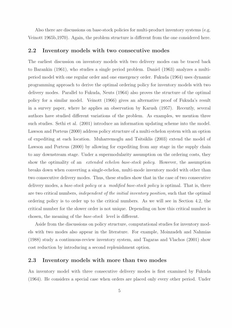
iii) Period 1.

W1(y1, q30) = (15)

189.5 − 10y1 − 10q30 if 0 6 q3

0 < 5.5, y1 6 10, I(a)

204.625 − 10y1 − 15.5q30 + 0.5(q3

0)2 if 5.5 6 q3

0 < 33.5, y1 6 12.75 − 0.5q30, I(b)

1175/3 − 10y1 − 80/3q30 + 2/3(q3

0)2 if q3

0 > 33.5, y1 6 (55 − 2q30)/3, I(c)

289.5 − 30y1 + (y1)2 − 10q3

0 if 10 < y1 6 15.5 − q30, II

259.75 − 61y1 + 2(y1)2 + 2q3

0y1 if max15.5 − q30, 12.75 − 0.5q3

0 < y1

−41q30 + (q3

0)2, 6 29.5 − q3

0, III

1400 − 120y1 + 3(y1)2 + 4q3

0y1 if y1 > max(55 − 2q30)/3, 29.5 − q3

0. IV

−100q30 + 2(q3

0)2

Figure 3: The cost function for period 1.

-50 -25

0

25

50 y1

0

10

20

30

40

s0

0

5000

10000

15000 W1

-50 -25

0

25

50 y1 -

6

1

3

0

q30

y1

I(a)

I(b)

I(c)

II

III

IV

2q30 + 3y1 = 55

q30 = 33.5

q30 + 2y1 = 25.5

q30 = 5.5

10 15.5 29.5

q30 + y1 = 29.5

q30 + y1 = 15.5

The optimal base-stock level for the fast mode in period 1 is

z11 =

10 if 0 6 q30 < 5.5,

12.75 − 0.5q30 if 5.5 6 q3

0 < 33.5,(55 − 2q3

0)/3 if q30 > 33.5.

The optimal post-order inventory positions are

(z1∗

1, z3∗

1) =

16

( 10, 24 + q3

0) if y1 6 10,

( y1, y1 + q3

0+ 14 ) if 10 < y1 6 15.5 − q3

0,

( y1, 29.5 ) if 15.5 − q3

0< y1 6 29.5 − q3

0,

( y1, y1 + q3

0) if y1 > 29.5 − q3

0

if 0 6 q3

0< 5.5,

( 12.75 − 0.5q3

0, 29.5 ) if y1 6 12.75 − 0.5q3

0,

( y1, 29.5 ) if 12.75 − 0.5q3

0< y1 6 29.5 − q3

0,

( y1, y1 + q3

0) if y1 > 29.5 − q3

0

if 5.5 6 q3

0< 33.5,

( (55 − 2q3

0)/3, 29.5 ) if y1 6 (55 − 2q3

0)/3,

( y1, y1 + q3

0) if y1 > (55 − 2q3

0)/3,

if q3

0> 33.5.

We notice that when 0 6 q30 < 5.5, there does not exist a base-stock level for the slow mode

in period 1. To see why, we take a closer look at what is happening in each period.

5.2 Discussion

We first examine how the demand is satisfied in each period. Observe that since the fast

ordering cost is the same for each period, it is never optimal to order on fast mode in an

earlier period and hold inventory to a later period. Likewise, it is never optimal to order on

fast mode in a later period and backlog demands from an earlier period. Suppose, for the

moment, that the initial inventory position y1 and in-transit order q30 are both zero.

• The demand in period 3 can be satisfied via the slow order Q31 in the first period and

the fast order Q13 in the third period. Since demand is deterministic, we know that

Q13 = 0 from Proposition 2. The quantity Q3

1 needed in period 3 is the minimizer to

q + (q − 10)2, which turns out to be 9.5. That is, at the end of the horizon, we would

like to have 0.5 units of backlog. Hence, we need a total of 29.5 units of the product

during the problem horizon.

• The demand in period 2 can be satisfied by the fast order Q12 in period 2. Also, we

can backlog some demand from period 2 to period 3 by ordering less Q12 but more Q3

1.

To do this, we save 9 dollars per unit ordering cost and pay the backlog cost. Thus,

the optimal quantity to backlog is the maximizer to 9q − q2, which is 4.5. Hence, Q12

should bring the inventory position for period 2 to at least 5.5 = (10 − 4.5).

• Now we come to period 1. Since the maximizer to 9q − q2 − (4.5 + q)2 is zero, it is not

optimal to backlog the demand in period 1 for two periods and satisfy it via Q31. We

should order 10 units of Q11.

17

It seems that the ideal order-up-to level for z31 would be 29.5, if the ordering policy for

the slow mode were to follow a base-stock policy. However, this cannot always be achieved

when q30 is low. Table 1 shows different inventory positions and corresponding optimal order

quantities over time when 0 6 q30 < 5.5.

Table 1: When 0 6 q30 < 5.5.

Period y1 (−∞, 10] (10, 15.5 − q30) [15.5 − q3

0 , 24.5 − q30 ] (24.5 − q3

0 , 29.5 − q30 ] (29.5 − q3

0 ,∞]

1 z11 10 10 10 10 10

Q1∗1 10 − y1 0 0 0 0

y1 + Q1∗1 + q3

0 10 + q30 y1 + q3

0 y1 + q30 y1 + q3

0 y1 + q30

Q3∗1 14 14 29.5 − y1 − q3

0 29.5 − y1 − q30 0

(z1∗1 , z3∗

1 ) (10, 24 + q30) (y1, y1 + q3

0 + 14) (y1, 29.5) (y1, 29.5) (y1, y1 + q30)

Period y2 q30 y1 + q3

0 − 10 y1 + q30 − 10 y1 + q3

0 − 10 y1 + q30 − 10

2 z12 5.5 5.5 −2.25 + 0.5y1 + 0.5q3

0 10 10

Q1∗2 5.5 − q3

0 15.5 − y1 − q30 0 0 0

z1∗2 5.5 5.5 y1 + q3

0 − 10 y1 + q30 − 10 y1 + q3

0 − 10

Period y3 9.5 9.5 9.5 9.5 y1 + q30 − 20

3 z13 5 5 5 5 5

Q1∗3 0 0 0 0 0

z1∗3 9.5 9.5 9.5 9.5 y1 + q3

0 − 20

End y4 −0.5 −0.5 −0.5 −0.5 y1 + q30 − 30

When y1 ∈ (−∞, 15.5 − q30) and q3

0 ∈ [0, 5.5), we have to order a positive Q12 in period

2 and order Q31 = 14(= 9.5 + 4.5) in period 1. In this case, the inventory position z3

1 does

not account for the value of Q12, since it only includes what is on-hand and what has been

ordered. So the optimal slow order Q31 in period 1 does not follow a base-stock policy. On the

other hand, when y1 > 15.5 − q30, there is no fast order placed in period 2. All the demands

have to be satisfied by the decision in period 1. In this case, the optimal inventory position

z31 should be as close to 29.5 as possible. One may think that if we modify the reference

inventory position y1 +q30 +Q1∗

1 to include the anticipated order Q12, then we could set 29.5 to

be the base-stock level for z31 , and have the optimal ordering policy to be a base-stock type

policy. While this could work in this deterministic demand example, it would not work in

the case of general stochastic demand. In this case, Q12 is a random variable at the beginning

of period 1, and no simple deterministic equivalence of this decision can be included in the

reference inventory position to restore the base-stock policy. We examine the stochastic

demand case in Section 6.

18

Table 2: When 5.5 < q30 6 33.5.

Period 1 y1 (−∞, 12.75 − 0.5q3

0] (12.75 − 0.5q3

0, 29.5 − q3

0] (29.5 − q3

0,∞]

z1

112.75 − 0.5q3

012.75 − 0.5q3

012.75 − 0.5q3

0

Q1∗

112.75 − 0.5q3

0− y1 0 0

y1 + Q1∗

1+ q3

012.75 + 0.5q3

0y1 + q3

0y1 + q3

0

Q3∗

116.75 − 0.5q3

029.5 − y1 − q3

00

(z1∗

1, z3∗

1) (12.75 − 0.5q3

0, 29.5) (y1, 29.5) (y1, y1 + q3

0)

Period 2 y2 2.75 + 0.5q3

0y1 + q3

0− 10 y1 + q3

0− 10

z1

2−2.25 + 0.5y1 + 0.5q3

0−2.25 + 0.5y1 + 0.5q3

012.5

Q1∗

20 0 0

z1∗

22.75 + 0.5q3

0y1 + q3

0− 10 y1 + q3

0− 10

Period 3 y3 9.5 9.5 y1 + q3

0− 10

z1

35 5 5

Q1∗

30 0 0

z1∗

39.5 9.5 y1 + q3

0− 10

End y4 −0.5 −0.5 y1 + q3

0− 30

As shown in Table 2, when 5.5 6 q30 6 33.5, demand in period 2 can be satisfied through

5.5 units from q30 and 4.5 units from Q3

1. Thus, no order in period 2 is needed and Q12 = 0.

Also, the remaining q30 − 5.5 can be allocated to satisfy the demand of either period 1 or of

period 3. In the former case, we backlog demand in period 1 and save the ordering cost for

Q11; in the latter case, we hold inventory at the end of period 2 and save the ordering cost

Q31. The marginal cost curve turns out be to the same for the two scenarios. Thus, we split

q30 − 5.5 evenly. As a result, we have 0.5q3

0 − 2.75 units of backlog at the end of period 1,

and order only 16.75 − 0.5q30(= 14 − (0.5q3

0 − 2.75)) units of Q31.

When q30 > 5.5, the fast order Q1

2 in period 2 is never placed, and optimal post-order

inventory position z31 should be as close to 29.5 as possible. Later we will see that such a

relationship between Q12 and z3

1 is not accidental. Since the value of q30 decides whether such

a situation would happen, 29.5 cannot be called a base-stock level rigourously according to

Definition 2. However, z31 = 29.5 is a base stock in the sense of Definition 1 when q3

0 > 5.5.

We now summarize our findings from this example:

• In general, the optimal ordering policy for an inventory system with two non-consecutive

modes is not a base-stock policy. Our example indicates that the base-stock policy fails

on the slow mode (the type 3 order).

• In our example, the base-stock policy fails to be optimal when

19

1. there are two non-consecutive delivery modes, and/or

2. demand is deterministic, and/or

3. all costs are stationary.

• The policy structure for period 1 is closely related to the size of the in-transit order q30

to be delivered after period 1. When q30 is large enough, the optimal ordering policy

follows a base-stock policy in the sense of Definition 1.

• Finally, we remark that the occurrence of the base-stock policy in period 1 coincides

with no fast order in period 2 under the optimal policy for this example.

6. Inventory Models with More than Two Modes

The example described in the last section is a special case of an inventory system with

multiple modes. The optimal ordering policies for inventory models with more than two

modes are no longer base-stock policies in general. The complexity of the problem with

more than two modes increases because the decision has to take into account the in-transit

order to be delivered in the future. A natural question to ask is when the optimal policy

follows a base-stock policy? If not, does the optimal ordering policy have some structure?

6.1 Separability and The Base-stock Policy

The following proposition states that in an optimal order policy, the first two modes follows

a base-stock policy.

Proposition 5 Define

P (y, p2, ..pN−1) = minF (z1, ..., zN )|z1> y, zj

> zj−1 + pj for j = 2, ..., N

where F (z1, ..., zN ) = G1(z1) + G2(z

2, ..., zN ) with G1(z1) convex in z1 and G2(z

2, ..., zN )

jointly convex in (z2, ..., zN ). Let (z1∗, ..., zN∗) be any solution to P (y, p2, ..pN−1). Then

there exist two reals z1 and z2 such that

z1∗ = z1 ∨ y, z2∗ = z2 ∨ (z1∗ + p2).

The proof of Proposition 5 will use the following lemma.

20

Lemma 1 Suppose G(x1, ..., xn) is jointly convex in (x1, ..., xn). Define G′(x1, ..., xk) =

minG(x1, ..., xn)|xj > xj−1 + aj for j = k + 1, ..., n for k = 1, ..., N . Then G′(x1, ..., xk) is

jointly convex in (x1, ..., xk).

Proof. We show that G′(x1, ..., xk) is jointly convex by induction on k. Clearly, when

k = N , G′(x1, ..., xN ) = G2(x1, ..., xN ) is jointly convex. Suppose that G′(x1, ..., xk+1) is

jointly convex in (x1, ..., xk+1) . Then,

G′(x1, ..., xk) = minG(x1, ..., xN )|xj> xj−1 + aj for j = k + 1, ..., N

= minG′(x1, ..., xk+1)|xk+1> xk + ak+1.

Now define xk+1(x1, ..., xk) = arg minxk+1 G′(x1, ..., xk+1), then

G′(x1, ..., xk) = G′(

x1, ..., xk+1(x1, ..., xk) ∨ (xk + ak+1))

.

Clearly, G′(

x1, ..., xk+1(x1, ..., xk))

is convex since the lower envelope of a convex function is

convex. Thus, G′(x2, ..., xk) is convex.

Proof of Proposition 5. By Lemma 1, we can rewrite problem P (y, p2, ..pN−1) as

P (y, p2, ..pN−1) = minG1(z1) + G′

2(z2)|z1

> y, z2> z1 + p1.

Denote z1, z2 and z1 as the unconstrained minimizer to G1(z1), G′

2(z2), and G1(z

1) +

G′2(z

1), respectively. Let z1 = z1 ∧ z1 and z2 = z2. Also note that

minz1>y

z2>z1+p1

G1(z1) + G′

2(z2)

= minz1>y

G1(z1) + G′

2

(

z2 ∨ (z1 + p2))

.

The function inside “min” on the right-hand side is convex in z1. We consider two cases.

Case 1: z1 + p2 6 z2.

First note that in this case z1 6 z1, z1 = z1. We have z1 + p1 6 z2. Thus, for any

z1 > y

G1(z1 ∨ y) + G′

2

(

z2 ∨ (y ∨ z1 + p2))

6 G1(z1 ∨ y) + G′

2

(

z2 ∨ (y ∨ z1 + p2))

.

To see the last inequality, we note that the right-hand side is convex in z1. If y 6 z1, the

right-hand side is minimized at z1 = z1 = z1. If y > z1, the right-hand side is minimized

at z1 = y. Hence, the minimizer is z1∗ = z1 ∨ y = z1 ∨ y and z2∗ = z2 ∨ (z1∗ + p2).

21

Case 2: z1 + p2 > z2.

In this case the minimizer must be such that z1∗ + p2 = z2∗. Note that z1 < z1 and

z2 < z1 + p2. So z1 = z1 and z2 = z2 < z1 + p2. Thus, for any z1 > y,

G1(z1 ∨ y) + G′

2(z1 ∨ y + p2) = G1(z

1 ∨ y) + G′2

(

z2 ∨ (z1 ∨ y + p2))

6 G1(z1 ∨ y) + G′

2

(

z2 ∨ (z1 + p2))

.

Similar to case 1, if y 6 z1, then the right-hand side is minimized at z1. Otherwise, it

is minimized at y. Hence, the minimizer is z1∗ = z1 ∨ y = z1 ∨ y and z2∗ = z1∗ + p2 =

z2 ∨ (z1∗ + p2).

Remark 4 Clearly, z1 is independent of y, and it depends on p2, ..., pN−1. z2 is independent

of y and p2, and it depends on p3, ..., pN−1. Since z2 is decided without any concern of the

first mode z1, (z1, z2) are base-stock levels in the sense of both Definitions 1 and 2. Note

that one could also take z2 as z2 ∨ z1. In this case, z2 = z2 ∨ z1 is a base stock according to

Definition 1, but not according to Definition 2.

The objective function Jk is clearly separable in the first two post-order inventory posi-

tions z1k and z2

k. This is why the base-stock policy is optimal when there are less than two

modes. The next result indicates that the optimality of a base-stock policy can always be

established when the objective function is separable in the post-order inventory positions.

Proposition 6 Consider the minimization problem

P(y, p2, ..., pN−1) = min

N∑

i=1

fi(zi)|z1

> y; zj+1> zj + pj+1 for 1 6 j < N ; zN

> zN−1

,

where fi(zi) for 1 6 i 6 N are convex functions. There exists a vector (z1, ..., zN ), such that

the solution (z1∗, ..., zN∗) to problem P(y, p2, ..., pN−1) takes the following form

z1∗ = z1 ∨ y, (16)

zj∗ = zj ∨ (zj−1∗ + pj) for 1 < j < N,

zN∗ = zN ∨ zN−1∗.

Moreover, z1 can be taken to be independent of y, and zj can be taken to be independent of

(y, p2, ..., pj).

22

Proof. Define fk,n(zk) = min∑N

j=k fj(zj)|zj+1 > zj + pj+1 for k 6 j < N ; zN > zN−1.

By Lemma 1, fk,n(zk) is convex in zk. Now we can show the result by induction.

When k = 1, take z1 as the unconstrained minimizer to f 1,n(z1). Then z1∗ = z1 ∨ y.

Note that z1 is independent of y. Suppose that zj is the unconstrained minimizer to f j,n(zj)

and zj∗ = zj ∨ (zj−1 + pj) for 1 < j 6 i. It is clear from Lemma 1 that (z1∗, ..., zi∗) is the

minimizer to min∑i−1

j=1 fj(zj) + f i,n(xi)|z

1 > y; zj+1 > zj + pj+1 for 1 6 j < i. Now take

zi+1 as the unconstrained minimizer to f i+1,n(zi+1). Then,

P(y, p2, ..., pN−1) = minz1>y,

zj>zj−1+pj,j=1,...,i+1

i∑

j=1

fj(zj) + f i+1,n(zi+1)

= minz1>y,

zj>zj−1+pj,j=1,...,i

i∑

j=1

fj(zj) + min

zi+1>zi+pi+1f i+1,n(zi+1)

= minz1>y,

zj>zj−1+pj,j=1,...,i

i∑

j=1

fj(zj) + f i+1,n(zi+1 ∨ (zi + pi+1))

.

Since the minimum on the right-hand side is attained at (z1∗, ..., zi∗), we deduce that zi+1∗ =

zi+1 ∨ (zi∗ + pj). Also note that zi+1 is independent of (pi+2, ..., pN−1).

Remark 5 The critical numbers (z1, ..., zN ) are base-stock levels in the sense of both defi-

nitions. Similar to the situation in two-mode case, one can take (z1, ..., zN ) as the solution

to P(−∞, p2, ..., pN−1), and show that the relationship in (16) still holds. In this case, the

critical numbers are base stocks only in the sense of Definition 1.

6.2 Generalization of Fukuda

The paper by Fukuda (1964) is probably the first and the only discussion on the policy

structure for inventory ordering system with more than two modes. He considers an in-

ventory system with three consecutive delivery modes. He shows that the optimal ordering

policy follows a base-stock policy when orders are only placed every other period. Fukuda’s

model is slightly different from the one described below. He does not consider demand fore-

cast updates. Instead, he assumes stationary ordering costs for each period, and costs are

discounted over time. In fact, the policy structure remains unchanged even without these

23

assumptions. The optimality equation in this case can be written as

Wk(yk; rk) = minz3k>z2

k>z1k>yk

c1k(z

1k − yk) + c2

k(z2k − z1

k) + c3k(z

3k − z2

k) + EHk+1(z1k − Dk)

+EHk+2(z2k − Dk − Dk+1) + EWk+2(z

3k − Dk − Dk+1; Rk+2).

It is clear that the decision variable for the second mode z2 and the third mode z3 are

separable in the cost function when orders can be placed only every other period. Thus, what

Fukuda does amounts to forcing separability, and therefore he gets the base-stock policy. His

result can actually be generalized by the following observation.

Proposition 7 If the first mode in period k + 1 is not used, then the first three modes in

period k have optimal base-stock levels.

Proof. If the first mode is not used in period k + 1, then the cost function for period k

can be written as

Jk(z1k, ...z

Nk ; rk) = c1

k(z1k − yk) +

N∑

j=2

cjk(z

jk − zj−1

k − pjk) + Hk(z

1k − Dk)

+Wk+1(z2k − Dk, z

3k − z2

k, ..., zNk − zN−1

k ; Rk+1)

= c1k(z

1k − yk) +

N∑

j=2

cjk(z

jk − zj−1

k − pjk) + EHk(z

1k − Dk) +

+E minz3k+1>z4

k−Dk,

zjk+1>z

j−1k+1+z

j+1k −z

jk,

c3k+1(z

3k+1 − z4

k + Dk) +N

∑

j=4

cjk+1(z

jk+1 − zj−1

k+1 − zj+1k + zj

k)

+EHk+1(z2k − Dk − Dk+1)

+EWk+2(z3k − Dk − Dk+1, z

3k+1 − z3

k + Dk + Dk+1, ..., zNk+1 − zN−1

k+1 ; Rk+1)

.

Clearly, the last expression is separable in (z1k, z

2k, z

3k). Hence, the result follows from Propo-

sition 6.

Remark 6 Note that this result cannot be generalized for more than three modes. That is,

if the first two modes in period k + 1 are not used, then the fourth mode in period k may not

have an optimal base stock. The reason is that EWk+2 depends on z3k.

Corollary 1 If the demand for period k is deterministic, and the second mode in period

k is an effective mode, then the first three modes in period k have base-stock levels.

24

We have seen an example in Section 5, in which the demand in each period is determin-

istic, and the second mode is not effective. In that example, the base-stock policy fail to be

optimal.

In the general case, the objective function is not completely separable in the post-order

inventory positions. For example, when we have three consecutive modes (z1, z2, z3), the

objective function is of the form G1(z1) + G2(z2, z3). Suppose that the unconstrained min-

imizers to G1(z1) and G2(z2, z3) are z1 and (z2, z3), respectively. If the optimal ordering

policy is a base-stock policy, then (z1, z2, z3) should be the optimal base-stock levels. A

necessary condition for the optimality of a base-stock policy is that z3 = arg minz3 G2(z2, z3)

for each z2 > z2. That is, the optimal base-stock level for type 3 order should not be af-

fected by increasing of the second inventory position from its base-stock level. However,

when G2(z2, z3) is jointly convex but not separable, this is hardly true. We illustrate the

idea through an example.

6.3 An Example with Three Consecutive Modes

Consider a three period example with following settings:

• There are three consecutive orders available in each period. We name them fast Q1,

medium Q2, and slow Q3.

• The demand D1 for the first period follows uniform distribution over [0, 20], and the

demands for the last two periods are deterministic D2 = D3 = 20.

• Holding and backlog costs at the end of each period are given by

H4(x) =

0 if x > 0,−10x if x < 0;

H3(x) =

3x if x > 0,−4x if x < 0;

H2(x) =

2x if x > 0,−3x if x < 0.

Note that at the end of the horizon, a penalty of 10 is charged for each unit of unsatisfied

demand, and the leftover inventory is of no value.

• Ordering costs are stationary over time and are given by

c1 = 3, c2 = 2 c3 = 1.

Note that the costs do not satisfy the conditions described in Proposition 3.

We first look at the cost function and optimal ordering policy in each period (details of this

example are available on Sethi’s website www.utdallas.edu/∼sethi).

25

i) Period 3.

Since the penalty cost is higher than the ordering cost and the leftover inventory is

worthless, it is optimal to keep the inventory position as close to the demand as possible.

Thus,

W3(y3) =

0 if y3 > 20,60 − 3y3 if y3 < 20.

The optimal base-stock level is z13 = z1

3 = 20.

ii) Period 2.

We first evaluate the objective function.

J2(z12 , z

22) = c1(z1

2 − y2) + c2(z22 − z1

2 − q31) + H3(z

12 − D) + W3(z

22 − D)

= −c1y2 − c2q31 + G1

2(z12) + G2

2(z22),

where

G12(z

12) = (c1 − c2)z1

2 + H3(z12 − D2)

=

80 − 3z12 if z1

2 < 20,−60 − 4z1

2 if z12 > 20,

G22(z

22) = c2z2

2 + W3(z22 − D2)

=

400 − 8z22 if z2

2 < 40,2z2

2 if z22 > 40.

The unconstrained minimizers to G12(z

12) and G2

2(z22) are z1

2 = 20 and z22 = 40, respec-

tively. We can further compute the optimal cost function for period 2 as

W2(y2, q31) = min

z12>y2,

z22>z1

2+q31

J2(z12 , z

22)

=

100 − 2q31 − 3y2 if q3

1 6 20, y2 6 20, (A)20 − 2q3

1 + y2 if 20 < y2 6 40 − q31, (B)

60 − 3y2 if q31 > 20, y2 6 20, (C)

−60 + 3y2 if y2 > max20, 40 − q31. (D)

The optimal base-stock levels are (z12 , z

22) = (z1

2 , z22) = (20, 40). Note that the demand

for period 2 and 3 are just satisfied in this situation.

26

Figure 4: The cost function for period 2.

0

20

40

60

y2

0

10

20

30

s1

0

50

100 W2

0

20

40

60

y2 -

6

]

0

q31

y2

A B

C D

20

q31 + y2 = 40

20 40

iii) Period 1.

The objective function for period 1 is given by

J1(z11 , z

21 , Q

31)

= c1(z11 − y1) + c2(z2

1 − z11 − q3

0) + c3Q31 + EH2(z

12 − D) + EW2(z

22 − D,Q3

1)

= −c1y1 − c2q30 + G1

1(z11) + G2

2(z21 , Q

31),

where

G1

1(z1

1) = (c1 − c2)z1

1+ EH2(z

1

1− D1)

=

40 − 3z1

1+ 0.15(z1

1)2 if 0 6 z1

16 20,

40 − 3z1

1if z1

1< 0,

−20 + 3z1

1if z1

1> 20,

and

G2

1(z2

1, Q3

1) = c2z2

1+ c3Q3

1+ EW2(z

2

1− D1, Q

3

1)

=

130 − z2

1− Q3

1if Q3

1< 20, z2

1< 20, (a)

230 − 9z2

1+ 0.15(z2

1)2 − 3Q3

1+ 0.1z2

1Q3

1if Q3

1< 20, 20 6 z2

1< 40 − Q3

1, (b)

250 − 9z2

1+ 0.15(z2

1)2 − 5Q3

1+ 0.1z2

1Q3

1+ 0.05(Q3

1)2 if Q3

1< 20, 40 − Q3

16 z2

1< 40, (c)

90 − z2

1+ 0.05(z2

1)2 − 5Q3

1+ 0.01z2

1Q3

1+ 0.05(Q3

1)2 if Q3

1< 20, 40 6 z2

1< 60 − Q3

1, (d)

90 − z2

1+ Q3

1if Q3

1> 20, z2

1< 20, (e)

150 − 71z2

1+ 0.15(z2

1)2 + Q3

1if Q3

1> 20, 20 6 z2

1< 40, (f)

−90 + 5z2

1+ Q3

1if z2

1> max40, 60 − Q3

1, (g)

The unconstrained minimizers to G11(z

11) and G2

1(z21 , Q

31) are z1

1 = 10 and (z21 , Q

31) =

(70/3, 20), respectively. Since the holding/backlog costs are linear, and we are not

27

in the situation described in Proposition 3, each type of order stipulates only for

the demand in the period the order arrives. It is understandable that the optimal

inventory position z11 for the type 1 order is the mean of D1 (since D1 follows a uniform

distribution) and the optimal slow order size Q31 is just D3. However, the optimal

inventory position z21 for type 2 order is not enough to satisfy the 20(= D2) units of

demand in period 2 on average. This is because D1 is stochastic. The realization of D1

could be less than 10 units. Hence we would like to order less than 20 units of type 2

order in period 1, since we can place a supplement type 1 order in period 2 if D1 turns

out to be high. Thus, the optimal z21 is 70/3, which is lower than 30.

Figure 5: The function G21(z

21 , Q

31).

-

6

• -R

R-

Q31

z210

20

ab

c

d

e f g

20 5040 60

Q3∗

1(z2

1)

( 70

3, 20)

j

-

6

-

z3∗1

z2∗10

20

703

50 60

z3∗

1(z2∗

1)

1303

50

30

Fig. 5 shows how the optimal slow order quantity changes with the optimal medium

inventory position. When 70/3 6 z2∗1 6 30, the slow order size is constant at 20 and the

slow inventory position is increasing with z2∗. Hence, the optimal ordering policy for

the slow order cannot be a base-stock policy if z2∗ ever falls below 30 (This also gives

a counter example to Lemma 1 in Zhang 1996). To check if the latter ever happens,

we need to compute the optimal cost function for period 1.

W1(y1, q30) =

28

340/3 − 2q30 − 3y1 if y1 6 10, q3

0 6 40/3, (a)

385/2 − 2q30 − 6y1 + 0.15(y1)

2 if 10 < y1 6 min20, 70/3 − q30, (b)

205/3 − 2q30 if 20 < y1 6 70/3 − q3

0 , (c)

150 − 9q30 + 0.15(q3

0)2 − 7y1 + 0.3q30y1 + 0.15(y1)

2 if max20, 70/3 − q30 < y1 6 30 − q3

0 , (d)

105 − 6q30 + 0.1(q3

0)2 − 4y1 + 0.2q30y1 + 0.1(y1)

2 if max20, 30 − q30 < y1 6 40 − q3

0 , (e)

−55 + 2q30 + 4y1 if max20, 40 − q3

0 < y1 6 50 − q30 , (f)

70 − 3q30 + 0.05(q3

0)2 − y1 + 0.1q30y1 + 0.05(y1)

2 if max20, 50 − q30 < y1 6 60 − q3

0 , (g)

−110 + 3q30 + 5y1 if y1 > max20, 60 − q3

0. (h)

380/3 − 4q30 + 0.075(q3

0)2 − 3y1 if y1 6 50/3 − 0.5q30 , 40/3 < q3

0 6 80/3. (i)

210 − 9q30 + 0.15(q3

0)2 − 13y1 + 0.3q30y1 + 0.3(y1)

2 if max50/3 − 0.5q30 , 70/3 − q3

0 < y1

6 min20, 30 − q30, (j)

165 − 6q30 + 0.1(q3

0)2 − 10y1 + 0.2q30y1 + 0.25(y1)

2 if max14 − 0.4q30 , 30 − q3

0 < y1

6 min20, 40 − q30, (k)

5 + 2q30 − 2y1 + 0.15(y1)

2 if max0, 40 − q30 < y1 6 min20, 50 − q3

0, (l)

130 − 3q30 + 0.05(q3

0)2 − 7y1 + 0.1q30y1 + 0.2(y1)

2 if max0, 50 − q30 < y1 6 min20, 60 − q3

0, (m)

−50 + 3q30 − y1 + 0.15(y1)

2 if y1 > max0, 60 − q30, (n)

42.5 + q30 − 3y1 if y1 6 35 − q3

0 , q30 > 35, (o)

116 − 3.6q30 + 0.06(q3

0)2 − 3y1 if y1 6 14 − 0.4q30 , 80/3 < q3

0 6 35, (p)

165 − 6q30 + 0.1(q3

0)2 − 10y1 + 0.2q30y1 + 0.1(y1)

2 if 35 − q30 < y1 6 min0, 30 − q3

0, (q)

5 + 2q30 − 2y1 if 30 − q3

0 < y1 6 min0, 40 − q30, (r)

130 − 3q30 + 0.05(q3

0)2 − 7y1 + 0.1q30y1 + 0.05(y1)

2 if 50 − q30 < y1 6 min0, 60 − q3

0, (q3)

−50 + 3q30 − y1 if 60 − q3

0 < y1 6 0. (t)

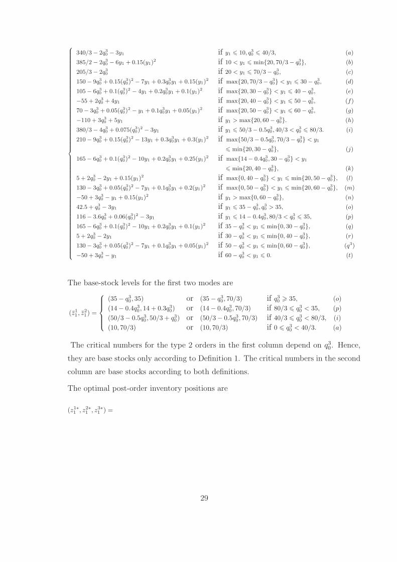
The base-stock levels for the first two modes are

(z1

1, z2

1) =

(35 − q3

0, 35) or (35 − q3

0, 70/3) if q3

0> 35, (o)

(14 − 0.4q3

0, 14 + 0.3q3

0) or (14 − 0.4q3

0, 70/3) if 80/3 6 q3

0< 35, (p)

(50/3 − 0.5q3

0, 50/3 + q3

0) or (50/3 − 0.5q3

0, 70/3) if 40/3 6 q3

0< 80/3, (i)

(10, 70/3) or (10, 70/3) if 0 6 q3

0< 40/3. (a)

The critical numbers for the type 2 orders in the first column depend on q30. Hence,

they are base stocks only according to Definition 1. The critical numbers in the second

column are base stocks according to both definitions.

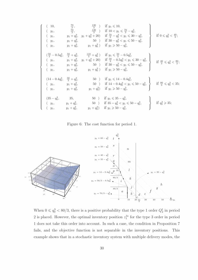
The optimal post-order inventory positions are

(z1∗

1, z2∗

1, z3∗

1) =

29

( 10, 70

3, 130

3) if y1 6 10,

( y1,70

3, 130

3) if 10 < y1 6 70

3− q3

0,

( y1, y1 + q3

0, y1 + q3

0+ 20) if 70

3− q3

0< y1 6 30 − q3

0,

( y1, y1 + q3

0, 50 ) if 30 − q3

0< y1 6 50 − q3

0,

( y1, y1 + q3

0, y1 + q3

0) if y1 > 50 − q3

0,

if 0 6 q3

0< 40

3;

( 50

3− 0.5q3

0, 50

3+ q3

0, 110

3+ q3

0) if y1 6 50

3− 0.5q3

0,

( y1, y1 + q3

0, y1 + q3

0+ 20) if 50

3− 0.5q3

0< y1 6 30 − q3

0,

( y1, y1 + q3

0, 50 ) if 30 − q3

0< y1 6 50 − q3

0,

( y1, y1 + q3

0, y1 + q3

0) if y1 > 50 − q3

0,

if 40

36 q3

0< 80

3;

(14 − 0.4q3

0, 50

3+ q3

0, 50 ) if y1 6 14 − 0.4q3

0,

( y1, y1 + q3

0, 50 ) if 14 − 0.4q3

0< y1 6 50 − q3

0,

( y1, y1 + q3

0, y1 + q3

0) if y1 > 50 − q3

0,

if 80

36 q3

0< 35;

(35 − q3

0, 35, 50 ) if y1 6 35 − q3

0,

( y1, y1 + q3

0, 50 ) if 35 − q3

0< y1 6 50 − q3

0,

( y1, y1 + q3

0, y1 + q3

0) if y1 > 50 − q3

0,

if q3

0> 35;

Figure 6: The cost function for period 1.

0

20

40

60

y1

0

10

20

30

40

s0

0

100

200

300

W1

0

20

40

60

y1

-

6

Y

Y y1 = 30 − q3

0y1 = 14 − 0.4q3

0

y1 = 50/3 − 0.5q3

0

y1 = 70/3 − q3

0

y1 = 60 − q3

0

y1 = 50 − q3

0

y1 = 40 − q3

0

y1 = 35 − q3

0

R

U

U

?

0

40/3

35

80/3

q30

y110 70

3

20 30 40 50 60

ab

cd e

fg

hi

j

k

l

m

n

o

p

q

r

s

t

When 0 6 q30 < 80/3, there is a positive probability that the type 1 order Q1

2 in period

2 is placed. However, the optimal inventory position z3∗1 for the type 3 order in period

1 does not take this order into account. In such a case, the condition in Proposition 7

fails, and the objective function is not separable in the inventory positions. This

example shows that in a stochastic inventory system with multiple delivery modes, the

30

Table 3: When 0 6 q30 < 40

3

Period y1 (−∞, 10] (10, 703− q3

0) [ 703− q3

0 , 30 − q30 ] (30 − q3, 40 − q3

0 ] (40 − q3, 50 − q30 ] (50 − q3

0 ,∞)

1 z11 10 10 10 10 10 10

Q1∗1 10 − y1 0 0 0 0 0

z1∗1 10 y1 y1 y1 y1 y1

z1∗ + q30 10 + q3

0 y1 + q30 y1 + q3

0 y1 + q30 y1 + q3

0 y1 + q30

z21

703

703

703

703

703

703

Q2∗1

403− q3

0403− q3

0 0 0 0 0

z2∗1

703

703

y1 + q30 y1 + q3

0 y1 + q30 y1 + q3

0

Q3∗1 20 20 20 50 − y1 − q3

0 50 − y1 − q30 0

z3∗1

1303

1303

y1 + q30 + 20 50 50 y1 + q3

0

Period y2703− d1

703− d1 y1 + q3

0 − d1 y1 + q30 − d1 y1 + q3

0 − d1 y1 + q30 − d1

2 z12 20 20 20 20 20 20

EQ1∗2

12518

12518

(40−y1−q3

0)2

40

(40−y1−q3

0,0)]2

400 0

z22 40 40 40 40 40 40

EQ2∗2 0 0 0 0 2.5

[max60−y1−q3

0,0]2

40

base-stock policy may fail when

(a) the holding/backlog costs are linear, and/or

(b) the demands are uniformly distributed.

In the examples discussed here, we have seen that the optimal ordering policies for in-

ventory models with multiple delivery modes are not base-stock policies in general. It would

be nice if the optimal policy had certain structure when it is not a base-stock policy. One

might observe from the two examples presented in this paper that when the type 3 orders

do not follow base-stock policy, the order quantity Q3∗1 ’s are always constants (14 in the first

example and 20 in the second one). However, this cannot be generalized. If we modify the

holding/backlog cost in period 3 to be H3(x) = 0.5x2 in the second example, Q3∗1 does not

have this property any longer. The corresponding G21(z

21 , Q

31) is given in Fig. 7.

7. Concluding Remarks

In this paper, we define the base-stock policy in the context of inventory systems with

multiple delivery modes and demand forecast updates. Two definitions are proposed. In

the first definition, the post-action inventory position(s) is(are) independent of the initial

inventory position. In the second definition, the post-action inventory position(s) is(are)

31

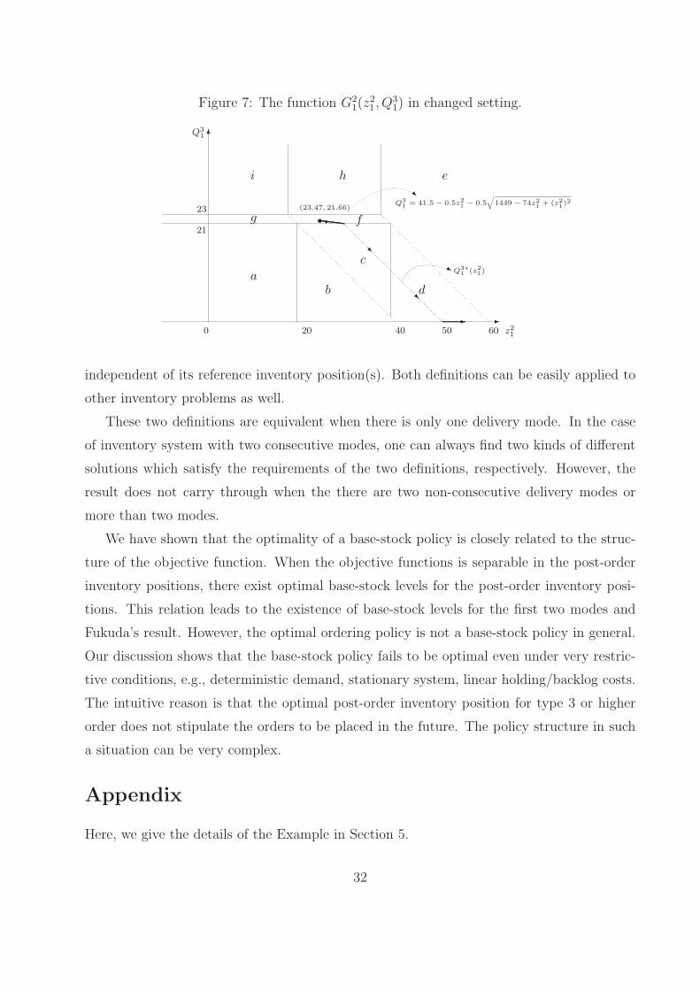
Figure 7: The function G21(z

21 , Q

31) in changed setting.

-

6

•-

R

R

-

Q31

z210

21

23

ab

c

d

g f

i h e

20 5040 60

Q3∗

1(z2

1)

(23.47, 21.66)Q3

1= 41.5 − 0.5z2

1− 0.5

√

1449 − 74z2

1+ (z2

1)2

j

R

independent of its reference inventory position(s). Both definitions can be easily applied to

other inventory problems as well.

These two definitions are equivalent when there is only one delivery mode. In the case

of inventory system with two consecutive modes, one can always find two kinds of different

solutions which satisfy the requirements of the two definitions, respectively. However, the

result does not carry through when the there are two non-consecutive delivery modes or

more than two modes.

We have shown that the optimality of a base-stock policy is closely related to the struc-

ture of the objective function. When the objective functions is separable in the post-order

inventory positions, there exist optimal base-stock levels for the post-order inventory posi-

tions. This relation leads to the existence of base-stock levels for the first two modes and

Fukuda’s result. However, the optimal ordering policy is not a base-stock policy in general.

Our discussion shows that the base-stock policy fails to be optimal even under very restric-

tive conditions, e.g., deterministic demand, stationary system, linear holding/backlog costs.

The intuitive reason is that the optimal post-order inventory position for type 3 or higher

order does not stipulate the orders to be placed in the future. The policy structure in such

a situation can be very complex.

Appendix

Here, we give the details of the Example in Section 5.

32

A. Period 3

W3(y3) = minz13>y3

c1(z13 − y3) + H(z1

3 − D)

= minz13>y3

10(z13 − y3) + (z1

3 − D)2

=

75 − 10y3 if y3 6 5,(y3 − 10)2 if y3 > 5.

The last equation follows from the fact that z13 = z1

3 = 5 is the minimizer to 10z13 +(z1

3 −D)2.

B. Period 2

W2(y2, q31) = min

z12>y2

J2(z12)

= minz12>y2

c1(z12 − y2) + H(z1

2 − D) + W3(z12 + q3

1 − D).

We need to consider two cases here to evaluate the objective function.

J2(z12) =

10(z12 − y2) + (z1

2 − 10)2 + 75 − 10(z12 + q3

1 − 10) if z12 + q3

1 − D 6 5,10(z1

2 − y2) + (z12 − 10)2 + (z1

2 + q31 − 10 − 10)2, if z1

2 + q31 − D > 5

=

275 − 10y2 − 20z12 + (z1

2)2 − 10q3

1 if z12 + q3

1 6 15,500 − 10y2 − 50z1

2 + 2(z12)

2 + 2z12q

31 − 40q3

1 + (q31)

2 if z12 + q3

1 > 15.

The unconstrained minimizer of the first piece of the function is 10 and that of the second

is 12.5 − 0.5q31. When q3

1 6 5, we have 10 + q31 6 15 and 12.5 − 0.5q3

1 + q31 6 15. Hence, the

optimal base-stock level is z12 = 10 when q3

1 6 5. When q31 > 5, we have z1

2 = 12.5 − 0.5q31.

Thus, the cost function can be written as in (14), and Fig. 4 is a plot of the function with

four regions.

C. Period 1

The optimal cost function for period 1 is given by

W1(y1, q30) = min

z11>y1,

Q31>0

J1(z11 , Q

31)

= minz11>y1,

Q31>0

c1(z11 − y1) + c3Q3

1 + H(z11 − D) + W2(z

11 + q3

0 − D,Q31).

33

We need to first examine the function J1(z11 , Q

31) in the four cases A, B, C, and D corre-

sponding to W2 given below. Functions and corresponding minimizers are subscripted A, B,

C, and D according to their respective cases.

C.1 Minimizer without considering y1

We first examine the objective function without considering the constraint that z11 > y1.

Case A z11 + q3

0 − D 6 10 (i.e. z11 + q3

0 6 20) and Q31 6 5.

J1A(z11 , Q

31) = 375 − 10y1 − 20z1

1 + (z11)

2 − 10q30 − 9Q3

1.

The minimizer is (z11A, Q3

1A) = (10 ∧ (20 − q30), 5).

(A.i) If q30 6 10, then the minimizer is (z1

1A, Q31A) = (10, 5), and the minimum cost is

JA(10, 5) = 230 − 10y1 − 10q30.

(A.ii) If q30 > 10, then the minimizer is (z1

1A, Q31A) = (20− q3

0, 5), and the minimum cost

is

JA(10, 5) = 330 − 10y1 − 30q30 + (q3

0)2.

Case B 10 < z11 + q3

0 − D 6 15 − Q31 (i.e. 20 < z1

1 + q30 6 25 − Q3

1).

J1B(z11 , Q

31) = 775 − 10y1 − 60z1

1 + 2(z11)

2 + 2z11q

30 + (q3

0)2 − 50q3

0 − 9Q31.

The minimizer is along the line z11 + q3

0 = 25 − Q31.

(B.i) If 0 6 q30 < 14.5, then the minimizer is (z1

1B, Q31B) = (20−q3

0, 5), and the minimum

cost is

J1B(z11B, Q3

1B) = J1B(20 − q30, 5) = 330 − 10y1 − 30q3

0 + (q30)

2.

(B.ii) If 14.5 6 q30 < 24.5, then the minimizer is (z1

1B, Q31B) = (12.75 − 0.5q3

0, 12.25 −

0.5q30), and the minimum cost is

JB(12.75 − 0.5q30, 12.25 − 0.5q3

0) = 224.875 − 10y1 − 15.5q30 + 0.5(q3

0)2.

(B.iii) If q30 > 24.5, then the minimizer is (z1

1B, Q31B) = (25 − q3

0, 0), and the minimum

cost is

JB(25 − q30, 0) = 525 − 10y1 − 40q3

0 + (q30)

2.

34

Case C z11 + q3

0 − D 6 12.5 − 0.5Q31 (i.e., z1

1 + q30 6 22.5 − 0.5Q3

1) and Q31 > 5.

J1C(z11 , Q

31) = 387.5 − 10y1 − 20z1

1 + (z11)

2 − 10q30 − 14Q3

1 + 0.5(Q31)

2.

The unconstrained minimizer to the function is (z11C , Q3

1C) = (10, 14).

(C.i) If q30 6 5.5, then the minimizer is (z1

1C , Q31C) = (10, 14), and the minimum cost is

JC(10, 14) = 189.5 − 10y1 − 10q30.

(C.ii) If 5.5 < q30 < 19, then the minimizer is (z1

1C , Q31C) = (1

3(41 − 2q3

0),13(53 − 2q3

0)),

and the minimum cost is

JC(1

3(41 − 2q3

0),1

3(53 − 2q3

0)) =629

3− 10y1 −

52

3q30 +

2

3(q3

0)2.

(C.iii) If q30 > 19, then the minimizer is (z1

1C , Q31C) = (20− q3

0, 5), and the minimum cost

is

JC(20 − q30, 5) = 330 − 10y1 − 30q3

0 + (q30)

2.

Case D z11 + q3

0 − D > max12.5 − 0.5Q31, 15 − Q3

1.

J1D(z11 , Q

31) = 1400 − 10y1 − 110z1

1 + 3(z11)

2 − 100q30 + 4z1

1q30 + 2z1

1Q31

+2(q30)

2 + 2q30Q

31 − 59Q3

1 + (Q31)

2.

The unconstrained minimizer takes the form z11D = (55−2q3

0−Q31D)/3 and Q3

1D = (59−

2z11D−2q3

0)/2, which can be solved to yield z11D = 12.75−0.5q3

0 and Q31D = 16.75−0.5q3

0.

(D.i) If q30 6 5.5, then the minimizer is (z1

1D, Q31D) = (1

3(41− 2q3

0),13(53− 2q3

0)), and the

minimum cost is

JD(1

3(41 − 2q3

0),1

3(53 − 2q3

0)) =629

3− 10y1 −

52

3q30 +

2

3(q3

0)2.

(D.ii) If 5.5 < q30 < 33.5, then the minimizer is (z1

1D, Q31D) = (1

4(51 − 2q3

0),14(67 − 2q3

0)),

and the minimum cost is

JD(1

4(51 − 2q3

0),1

4(67 − 2q3

0)) = 204.625 − 10y1 − 15.5q30 + 0.5(q3

0)2.

(D.iii) If q30 > 33.5, then the minimizer is (z1

1D, Q31D) = (1

3(55−2q3

0), 0), and the minimum

cost is

JD(1

3(55 − 2q3

0), 0) =1175

3− 10y1 −

80

3q30 +

2

3(q3

0)2.

35

Table 4: The minimizer of the function in each region.

q3

0[0, 5.5] (5.5, 10] (10, 14.5] (14.5, 19] (19, 24.5] (24.5, 35.5] (35.5,∞)

J1A z1

1A20 − q3

010

Q3

1A5

J1B z1

1B20 − q3

012.75 − 0.5q3

025 − q3

0

Q3

1B5 12.25 − 0.5q3

00

J1C z1

1C10 (41 − 2q3

0)/3 20 − q3

0

Q3

1C14 (53 − 2q3

0)/3 5

J1D z1

1D(41 − 2q3

0)/3 12.75 − 0.5q3

0(55 − 2q3

0)/3

Q3

1D(53 − 2q3

0)/3 16.75 − 0.5q3

00

We summarize the results in the following table.

Now we are ready to determine the optimal ordering policy when y1 is small enough. We

start by dividing the plane according to the value of q30.

Case I 0 6 q30 6 5.5.

J1A(z11A, Q3

1A) = J1A(10, 5) = 230 − 10y1 − 10q30, (17)

J1B(z11B, Q3

1B) = J1B(20 − q30, 5) = 330 − 10y1 − 30q3

0 + (q30)

2, (18)

J1C(z11C , Q3

1C) = J1C(10, 14) = 189.5 − 10y1 − 10q30, (19)

J1D(z11D, Q3

1D) = J1D((41 − 2q30)/3, (53 − 2q3

0)/3)

= 629/3 − 10y1 − 52/3q30 + 2/3(q3

0)2. (20)

We do some simple comparisons

J1D(z11D, Q3

1D) − J1C(z11C , Q3

1C) = (11 − 2q30)

2/6 > 0,

J1B(z11B, Q3

1B) − J1A(z11A, Q3

1A) = (q30 + 10)2 > 0,

J1A(z11A, Q3

1A) − J1C(z11C , Q3

1C) = 40.5 > 0.

Thus, (z11 , Q

31) = (z1

1C , Q31C) = (10, 14). When y1 6 (41 − 2q3

0)/3, we have

W1(y1, q30) = 189.5 − 10y1 − 10q3

0.

Case II 5.5 < q30 6 33.5.

36

When 5.5 < q30 6 10, the functions J1C and J1D are different from Case I.

J1C(z11C , Q3

1C) = J1C((41 − 2q30)/3, (53 − 2q3

0)/3) = 629/3 − 10y1 − 52/3q30 + 2/3(q3

0)2,

J1D(z11D, Q3

1D) = J1D(12.75 − 0.5q30, 16.75 − 0.5q3

0) = 204.625 − 10y1 − 15.5q30 + 0.5(q3

0)2.

Compare minima of the functions:

J1D(z11D, Q3

1D) − J1C(z11C , Q3

1C) = −(11 − 2q30)/24 < 0,

J1A(z11A, Q3

1A) − J1C(z11C , Q3

1C) = −(6.75 + 2(q30 − 5.5)2)/3 < 0.

Thus, (z11 , Q

31) = (z1

1D, Q31D) = (12.75− 0.5q3

0, 16.75− 0.5q30). When y1 6 12.75− 0.5q3

0,

we have

W1(y1, q30) = 204.625 − 10y1 − 15.5q3

0 + 0.5(q30)

2.

When 10 < q30 6 33.5, we can compare the functions in a similar way, and find that

(z11 , Q

31) = (12.75 − 0.5q3

0, 16.75 − 0.5q30) also is a minimizer in this case.

Case III q30 > 33.5.

The function J1D becomes

J1D((55 − 2q30)/3, 0) = 1175/3 − 10y1 − 80/3q3

0 + 2/3(q30)

2.

Comparing with J1A, J1B and J1C , we find that the optimal (z11 , Q

31) = (z1

1D, Q31D) =

((55 − 2q30)/3, 0), and the optimal cost function is

W1(y1, q30) = 1175/3 − 10y1 − 80/3q3

0 + 2/3(q30)

2.

C.2 Incorporating y1 into the decision

Now we incorporate y1 in our decision by considering the situation when y1 > z11 , where z1

1

is as computed in the previous section. Thus, the only problem left to solve is the one of

choosing an optimal Q31 for the given y1.

1. 10 < y1 < 20 − q30. We compare three functions J1A, J1C and J1D. With an abuse of

notation, we denote Q31i as the optimal value of Q3

1 in region i with respect to a given

37

value of y1.

J1A(y1, Q31A) = J1A(y1, 5) = 330 − 30y1 + y2

1 − 10q30,

J1C(y1, Q31C) =

J1C(y1, 14) if y1 + q30 6 15.5

J1C(y1, 45 − 2y1 − 2q30) if y1 + q3

0 > 15.5

=

289.5 − 30y1 + y21 − 10q3

0 if y1 + q30 6 15.5,

770 − 92y1 + 3y21 + 4q3

0y1 − 72q30 + 2(q3

0)2 if y1 + q3

0 > 15.5,

J1D(y1, Q31D) = J1D(y1, 29.5 − y1 − q3

0)

= 529.75 − 61y1 + 2y21 + 2q3

0y1 − 41q30 + (q3

0)2.

(a) When y1 + q30 6 15.5, we have

J1A(y1, 5) − J1C(y1, 14) > 0,

J1D(y1, 29.5 − y1 − q30) − J1C(y1, 14) = (21.864 − y1 − q3

0)(y1 + q30 − 9.13604) > 0.

So the slow order is Q31 = 14, and the cost function is

W1(y1, q30) = 289.5 − 10q3

0 − 30y1 + y21.

(b) When y1 + q30 > 15.5,

J1A(y1, 5) − J1C(y1, 45 − 2y1 − 2q30) = −2(y1 + q3

0 − 20)(y1 + q30 − 11) > 0.

J1D(y1, 29.5 − y1 − q30) − J1C(y1, 45 − 2y1 − 2q3

0) = −(y1 + q30 − 15.5)2

6 0

So the optimal slow order is Q31 = 29.5 − y1 − q3

0, and the cost function is

W1(y1, q30) = 529.75 − 61y1 + 2y2

1 + 2q30y1 − 41q3

0 + (q30)

2.

2. y1 > max20 − q30, (55 − 2q3

0)/3, 12.75 − 0.5q30.

We compare the two functions J1B and J1D.

J1B(y1, Q31B) = J1B(y1, 25 − y1 − q3

0)

= 550 − 61y1 + 2y21 + 2q3

0y1 − 41q30 + (q3

0)2 for 20 < y1 + q3

0 < 25,

J1D(y1, Q31D) =

J1D(y1, 29.5 − y1 − q30) for y1 + q3

0 6 29.5J1D(y1, 0) for y1 + q3

0 > 29.5

=

529.75 − 61y1 + 2y21 + 2q3

0y1 − 41q30 + (q3

0)2 for y1 + q3

0 6 29.51400 − 120y1 + 3y2

1 + 4q30y1 − 100q3

0 + 2(q30)

2 for y1 + q30 > 29.5

Observe that if 20 < y1 + q30 < 25, then J1B(y1, 25− y1 −Q3

1) > J1D(y1, 29.5− y1 − q30).

38

(a) When y1 + q30 6 29.5,

W1(y1, q30) = 529.75 − 61y1 + 2y2

1 + 2q30y1 − 41q3

0 + (q30)

2.

(b) When y1 + q30 > 29.5,

W1(y1, q30) = 1400 − 120y1 + 3y2

1 + 4q30y1 − 100q3

0 + 2(q30)

2.

Finally, we can write the complete cost function for period 1 as in (15).

References

Arrow, K., T. Harris and J. Marschak. 1958. Optimal inventory policy. Econometrica.

19(3) 250-272.

Barankin, E. W. 1961. A delivery-lag inventory model with an emergency provision (the

one-period case). Naval Res. Logist. Quart. 8(3) 258-311.

Bellman, R., I. Glicksberg and O. Gross. 1955. On the optimal inventory equation. Man-

agement Sci. 2(1). 83-104.

Cheng, F. and S. P. Sethi. 1999. A periodic review inventory model with demand influenced

by promotion decisions. Management Sci. 45(11). 1510-1523.

Daniel, K. H. 1963. A delivery-lag inventory model with emergency. H. E. Scarf, D. M.

Gilford and M. W. Shelly (eds.) Multistage Inventory Models and Techniques. Stanford

University Press, Stanford, CA.

Dvorerzky, A., J. Kiefer and J. Wolfowitz. 1952. The inventory problem: I. case of known

distribution of demand. Econometrica. 20(2). 187-222.

——, ——, ——. 1952. The inventory problem: II. case of unknown distribution of demand.

Econometrica. 20(3). 451-466.

Feng, Q., G. Gallego, Sethi, S. P., H. Yan and H. Zhang. 2003. A periodic review inven-

tory model with three consecutive delivery modes and forecast updates, working paper.

University of Texas at Dallas, TX.

Fukuda, Y. 1964. Optimal policies for the inventory problem with negotiable leadtime.

Management Sci. 10(4). 690-708.

Gaver, D. P., Jr. 1959. On base-stock level inventory control. Opns. Res. 7(6) 689-703.

39

——. 1961. Operating characteristics of a simple production, inventory-control model.

Opns. Res. 9(5) 635-649.

Iglehart, D.and S. Karlin. 1962. Optimal Policy for Dynamic Inventory Process with Non-

stationary stochastic demands. K. Arrow, S. Karlin, H. Scarf (eds.) Studies in Applied

Probability and Management Sci. Stanford University Press, Stanford, CA. Chapter 8.

Karlin, S. 1958. Optimal inventory policy for the Arrow-Harris-Marschak dynamic model.

K. Arrow, S. Karlin and H. Scarf (eds.) Studies in the Mathematical Theory of Inventory

and Production. Stanford University Press, Stanford. Chapter 9.

——. 1960. Dynamic inventory policy with varying stochastic demands. Management Sci.

6(3) 231-258.

—— and H. Scarf. 1958. Inventory models of the Arrow-Harris-Marschak type with time

lag. K. Arrow, S. Karlin and H. Scarf (eds.) Studies in the Mathematical Theory of

Inventory and Production. Stanford University Press, Stanford, CA. Chapter 10.

Karush, W. 1957. Mathematical programming and service scheduling. Management Sci.

3(2). 140-148.

Lawson, D. G. and E. L. Porteus. 2000. Multistage inventory management with expediting.

Opns. Res. 48 878-893.

Moinzadeh, K. and S. Nahmias. 1988. A Continuous review model for an inventory system

with two supply modes, Management Sci., 34, 761-773.

Muharremoglu, A. and J. N. Tsitsikli Dynamic leadtime management in supply chains,

working paper.

Neuts, M. 1964. An inventory model with an optional time lag. J. SIAM. 12(1). 179-185.

Porteus, E.L. 2002. Stochastic Inventory Theory. Stanford University Press, Stanford, CA.

Sethi, S. P. and F. Cheng. 1997. Optimality of (s, S) policies in inventory models with

Markovian demand. Opns. Res., 45(6), 931-939.

——, H. Yan and H. Zhang. 2001. Peeling Layers of an Onion: A periodic review inventory

model with multiple delivery models and forecast updates. J. Optimiz. Theory Appl.,

108, 253-281.

Song, J-S. and P. Zipkin. 1993. Inventory control in a fluctuating demand environment.

Opns. Res. 41(2). 351-370.

40

Tagaras, G. and D. Vlachos. 2001. A periodic review inventory system with emergency

replenishments, Management Sci., 47,415-429.

Topkis, D. M. 1968. Optimal ordering and rationing policies in a nonstationary dynamic

inventory model with n demand classes. Management Sci. 15(3) 160-176.

Veinott, A. 1965a. Optimal policy in a dynamic, single product , nonstationary inventory

model with several demand classes. Opns. Res. 13(5) 761-778.

——. 1965b. Optimal policy for multi-product, dynamic, nonstationary inventory problem.

Management Sci. 12(3) 206-222.

——. 1966. The status of mathematical inventory theory. Management Sci. 12(11). 745-

777.

——. 1970. A correction for “Optimal policy for multi-product, dynamic, nonstationary

inventory problem”. Management Sci. 16(7))

Zhang, V. L. 1996. Ordering policies for an inventory system with three supply modes, Naval

Res. Logist., 43, 691-708.

41