Optimal Climate Policies in a Dynamic

Multi-Country Equilibrium Model∗

Elmar Hillebrand† Marten Hillebrand‡

March 31, 2017

Abstract

This paper develops a dynamic general equilibrium model with an arbitrary num-

ber of different regions to study the economic consequences of climate change

under alternative climate policies. Regions differ with respect to their state of

economic development, factor endowments, and climate damages and trade on

global markets for capital, output, and exhaustible resources. Our main result de-

rives an optimal climate policy consisting of an emissions tax and a transfer policy.

The optimal tax can be determined explicitly in our framework and is independent

of any weights attached to the interests of different countries. Such weights only

determine optimal transfers which distribute tax revenues across countries. We

infer that the real political issue is not the tax policy required to reduce global

warming but rather how the burden of climate change should be shared via trans-

fer payments between different countries. We propose a simple transfer policy

which induces a Pareto improvement relative to the Laissez faire solution.

JEL classification: E10, E61, H21, H23, Q43, Q54

Keywords: Multi-region model; Dynamic equilibrium; Climate change; Optimal climate

tax; Optimal transfer policy; Emissions trading system.

First version: Dec. 2015, this version: March 2017.

∗Acknowledgements. We would like to thank Philipp Harms, Tomoo Kikuchi, Oliver Saffran, and

KlausWalde for very helpful discussions and suggestions and seminar participants at various conferences

and research seminars for valuable comments.†EEFA Research Institute, Muenster, Germany, email: e.hillebrand@eefa.de‡Gutenberg School of Management & Economics, Mainz University, Mainz, Germany, email:

mhillebr@uni-mainz.de (corresponding author).

Introduction

Global warming and its consequences for the world economy constitute one of the biggest

challenges of the twenty-first century. While the fact that climate change is mainly driven

by man-made emissions of carbon-dioxide (CO2) seems now largely undisputed, political

measures to reduce these emissions and limit climate damages remain controversial and

are also difficult to implement. An obvious reason for this is that climate change is a

global problem and climate policies must be coordinated and implemented by different

countries with heterogeneous characteristics each acting in their own economic interest

which induces well-known problems such as free-riding, etc. cf. Nordhaus (2015).

This general insight suggests that a theoretical evaluation of alternative climate policies

should take place in a framework with multiple regions or countries which are politically

autonomous and can differ with respect to their economic and other characteristics. The

present paper develops such a model to analyze a number of intriguing questions raised

in the political debate such as: What is the optimal tax policy to curb emissions? How

should this tax differ across regions depending on heterogeneities in economic develop-

ment, productivity, climate damages, etc.? What is the optimal path of production,

emissions, and climate damage in each region and the optimal extraction of fossil re-

sources? Which mix of dirty and clean technologies should each region adopt to produce

energy goods and services for production?

Intuitively, one might expect that the answers to these and related questions depend on

the weighting of the interests of different regions. Our main result in this paper shows

that this intuition is false: All answers to the previous questions are uniquely deter-

mined and independent of such weights. In particular, there is no trade-off between the

interests of different regions. This insight is based on general structural properties which

extend beyond the specific framework employed in this paper. As almost all existing

climate models with multiple regions derive optimal climate policies based on (essen-

tially arbitrary) weights assigned to each region (see, e.g., Nordhaus & Yang (1996)),

our paper provides a very general theoretical contribution to the existing literature.

Conceptually, the model developed in this paper uses dynamic general equilibrium the-

ory to obtain an internally consistent economic framework with explicit market struc-

tures and price formation. The economic part is complemented by a climate model

describing how emissions determine atmospheric concentration of carbon dioxide and

the resulting damages on the economy. With these features, our model falls into the

class of integrated assessment (IA) models which incorporate the full interactions be-

tween climate variables and the economic production process.

Most of the existing IA-models are based on the RICE/DICE framework pioneered by

Nordhaus (1977) and further developed in Nordhaus & Yang (1996). The numerous

extensions and refinements of the RICE/DICE model are comprehensively surveyed

in Nordhaus (2011) and, more recently, in Hassler et al. (2016). A typical feature

1

of RICE/DICE-based models stressed in Hassler et al. (2016) is that their solutions

are essentially derived as planning problems making only limited use of dynamic general

equilibrium theory used in modern macroeconomics. As a consequence, a major problem

with the planning approach is the absence of market structures. Among other things,

this makes it difficult to study the response of private agents to arbitrary climate policies

and, therefore, to evaluate the economic consequences of possibly non-optimal policies.

An alternative framework taking full advantage of dynamic general equilibrium theory is

developed in Golosov et al. (2014), henceforth GHKT, who study a single-region model

of the world economy. Their main theoretical result is an explicit formula for the optimal

tax on fossil emissions. An extension of the GHKT model to a two-region framework is

developed in Hassler & Krusell (2012), see also Hassler, Krusell & Olovsson (2010). To

preserve analytical tractability, they impose strong restrictions on trade between regions

which are only allowed to trade fossil energy inputs.

The framework developed in this paper features an arbitrary number of regions which

can differ along various dimensions including factor endowments, productivity, natural

resources, and climate damages. Conceptually, it retains the virtues of DSGE modelling

from GHKT while allowing for more realistic trade between regions than in Hassler &

Krusell (2012). This is accomplished by explicitly separating the resource stage at which

fossil resources are extracted and the energy stage at which energy goods and services

are produced. Trade of exhaustible resources is unrestricted in our model while trading

of energy outputs is confined to the domestic market. In addition, our model includes an

international asset market which permits intertemporal borrowing and lending between

regions which is excluded in Hassler & Krusell (2012). While capital is perfectly mobile

in our model, labor can only be allocated within each region, which is the traditional

Ricardian assumption in trade theory. Modelling the energy stage explicitly also allows

us to study how climate policies induce transitions from dirty to clean technologies and

affect the energy mix in each region. An extensive numerical study of these questions

is offered in a companion paper Hillebrand & Hillebrand (2017).

With the previous features, our model is general enough to incorporate various types

of heterogeneity which are potentially important in the political discussion on climate

change. At the same time, it remains analytically tractable and permits the derivation

of theoretical results. Our main result establishes the existence of an optimal climate

policy consisting of an optimal tax on emissions and a transfer policy which determines

the distribution of tax revenue across regions via transfers. The optimal tax is uniquely

determined and independent of any weights attached to the welfare/utility of different

regions. It determines all equilibrium variables except for the distribution of world

consumption across regions which depends on the transfer policy. It is this result that

led us to claim that the questions raised above can be uniquely answered. Moreover,

we can characterize the optimal tax policy explicitly in our model to obtain an intuitive

and simple generalization of the tax formula derived in GHKT to a multi-region setting.

2

Our main result therefore shows that the efficiency issue of how to tax emissions can

strictly be separated from the distributional issue how tax revenue should be shared

across countries via transfers to induce a desired distribution of world consumption.

Based on this findings, our analysis suggests that the real political issue is not the tax

policy required to reduce global warming but rather how the burden of climate change

should be shared via transfer payments between different countries. Only the choice

of an appropriate transfer scheme induces a trade-off between the interests of different

regions and, therefore, should be the subject of negotiations during the political process.

As our final main result, we propose a simple transfer policy under which each region

is strictly better off relative to the Laissez faire case where no measures against climate

change are taken. Our transfer policy thus satisfies the property of individual rationality

discussed, e.g., in Eyckmans & Tulkens (2003)) which seems a minimal requirement for

a climate policy to be successfully implemented by each region.

The paper is organized as follows. Section 1 introduces the model. The decentralized

equilibrium solution and its properties under different climate policies are studied in

Section 2. Section 3 studies optimal allocations obtained as solutions to a planning

problem. The existence and form of optimal climate policies which implement the

optimal solution as an equilibrium allocation is studied in Section 4. Section 5 concludes,

mathematical results and proofs can be found in the Appendix.

1 The Model

1.1 World economy

The world economy is divided into L ≥ 1 regions, indexed by ℓ ∈ L := {1, . . . , L}.

Each region ℓ ∈ L pursues its own interests and takes autonomous political decisions.

Although each region typically represent unions or groups of different countries, we will

nevertheless refer to region ℓ as a country. Regions are geographically or institutionally

separated, which imposes certain restrictions on trade between them.

The production process in each region ℓ ∈ L decomposes into three stages. The final sec-

tor produces a consumable output commodity based on a set of inputs including energy

goods and services. The second stage consists of a collection of energy sectors which

produces these goods and services based either on renewable or exhaustible resources.

The third stage is represented by the resource sectors which extract the domestic stock

of exhaustible resources.

These different production stages together with a global climate model and a description

of the consumption sector in each region constitute the main building blocks of our model

which will be described in detail in the following sections.

3

1.2 Production sectors

Time is discrete and indexed by t ∈ {0, 1, 2, . . .}. There are I + 1 production sectors in

each region ℓ ∈ L which are identified by the index i ∈ I0 := {0, 1, . . . , I}. Sector i = 0

is the final sector while i ∈ I := {1, . . . , I} identifies the different energy sectors. Each

sector i ∈ I0 consist of a single representative firm which employs labor N ℓi,t ≥ 0 and

capital Kℓi,t ≥ 0 as production factors in period t.

Final sector

Sector i = 0 in region ℓ ∈ L produces final output in period t using the technology

Y ℓt = (1−Dℓ

t)Qℓ0,tF0(K

ℓ0,t, N

ℓ0,t, (E

ℓi,t)i∈I). (1)

Here, (Eℓi,t)i∈I is as collection of energy inputs used in addition to labor and capital in

production. The term Qℓ0,t > 0 in (1) is an exogenous, possibly time- and region-specific

productivity parameter which is diminished by damages due to climate change. The

latter is measured by a damage index Dℓt ∈ [0, 1[ which will be a function of total CO2

concentration in the atmosphere to be specified below. Finally,

Energy sectors

Energy is supplied by sectors i ∈ I. Their outputs should be broadly interpreted as

energy goods like electricity and heat or services like transportation. We distinguish

’exhaustible’ and ’renewable’ energy sectors depending on whether they base their pro-

duction on an exhaustible resource like coal, oil, and natural gas or a renewable resource

like wind, water, and solar energy.

Let Ix ⊂ I denote the subset of exhaustible energy sectors. Each such sector i ∈ Ix is

uniquely identified by the underlying resource on which production is based (like ’coal’

used for ’coal-fired power generation’ or ’oil’ used to provide ’fuel-based transportation

services’). The amount of exhaustible resource i ∈ Ix used in region ℓ ∈ L at time t is

denoted by Xℓi,t ≥ 0. Exhaustible resources are typically an essential input to production

in the respective sector and generate emissions proportional to their usage in production.

Energy sectors thus represent the production stage at which emissions are potentially

generated. Sectors which employ renewable sources do not cause emissions.1

With the previous distinction, the technology used by an exhaustible energy sector i ∈ Ix

to produce energy output in period t takes the form

Eℓ,si,t = Qℓ

i,tFi(Kℓi,t, N

ℓi,t, X

ℓi,t) (2)

while production in a renewable energy sector i ∈ I\Ix in period t is given by

Eℓ,si,t = Qℓ

i,tFi(Kℓi,t, N

ℓi,t). (3)

1This abstracts from emissions generated from using renewable resources like biomass, etc. which

are negligible relative to emissions from fossil fuels.

4

Similar to (1), both specifications (2) and (3) allow for time- and region-specific produc-

tivity Qℓi,t. In general, a higher productivity Qℓ

i,t > Qℓ′

i,t may reflect a more developed

technology in region ℓ relative to ℓ′ or the fact that conditions to produce energy of type

i ∈ I are more favorable in region ℓ than in ℓ′ due to geographic conditions, etc.2

Technology and productivity

Denoting by Qt := (Qℓi,t)(ℓ,i)∈L×I0

the world productivity vector in period t ≥ 0, we

assume that the evolution of the sequence (Qt)t≥0 is determined exogenously. The

remainder imposes the following standard restrictions on production technologies (1),

(2), and (3). The Inada condition ensures that each factor is employed in production.

Assumption 1

Each production function Fi : Rni

+ −→ R+, i ∈ I0 is linear homogeneous, strictly

increasing, concave, and C2 on Rni

++. The first partial derivatives satisfy the Inada-

condition limzmց0 ∂zmFi(z1, . . . , zni) = ∞ ∀z = (z1, . . . , zni

) ∈ Rni

++ and m = 1, . . . , ni.

Resource sectors

Resource sectors are uniquely identified by the energy sector i ∈ Ix which uses this

resource in production. In each region ℓ ∈ L, there exists a single firm which extracts

resources of type i ∈ Ix and supplies them to the global resource market. The amount

of resource i extracted and supplied in period t is denoted Xℓ,si,t ≥ 0 (to be distinguished

from the amount Xℓi,t demanded by energy sector i ∈ Ix in that region). Resource

firms face constant per unit extraction costs ci ≥ 0 and take the initial resource stock

Rℓi,0 ≥ 0 as a given parameter.3 Feasible extraction plans are thus non-negative sequences

(Xℓ,si,t )t≥0 which respect the feasibility constraint

∞∑

t=0

Xℓ,si,t ≤ Rℓ

i,0. (4)

To avoid trivialities, we impose the initial condition∑

ℓ∈LRℓi,0 > 0, i.e., initial world

resources are strictly positive for all i ∈ Ix. It may, however, be the case that Rℓi,0 = 0

in which case region ℓ does not own any resources of type i.

1.3 Climate model

Emissions of CO2 are generated by using (’burning’) exhaustible resources like coal, oil,

and gas to produce energy. Thus, emission occur at the energy stage in production. The

2For example, a solar energy plant located in the Sahara seems likely to produce more electricity

output than an identical plant located in a northern European region like Norway while the opposite

holds in the case with hydroelectric power generation.3The assumption of constant extraction costs is a compromise between falling costs due to techno-

logical progress assumed in GHKT and extraction costs which increase with the scarcity of the resource

as discussed in Hotelling (1931). Our model should be amendable to extensions in either direction.

5

amount of CO2 generated by using one unit of exhaustible resource i ∈ Ix is physically

determined by its carbon-content ζi ≥ 0. In particular, ζi = 0 if the resource does no

generate emissions, like uranium in the case of nuclear energy production.4

Summing the different types of exhaustible resource inputs weighted by their respective

carbon content over all regions one obtains the total emissions of CO2 in period t as

Zt :=∑

ℓ∈L

∑

i∈Ix

ζiXℓi,t. (5)

Adopting the specification from GHKT, the climate state in period t consists of per-

manent and non-permanent CO2 in the atmosphere and is denoted by St = (S1,t, S2,t).

Given the sequence of emissions {Zt}t≥0 determined by (5), the climate state evolves as

S1,t = S1,t−1 + φLZt (6a)

S2,t = (1− φ)S2,t−1 + (1− φL)φ0Zt (6b)

Specification (6) assumes that a share 0 ≤ φL < 1 of emissions become permanent CO2.

Out of the remaining emissions, a share φ0 becomes non-permanent CO2 which decays

at constant rate 0 < φ < 1 while the remaining share 1− φ0 leaves the atmosphere (see

GHKT for details). Total concentration of CO2 at time t is thus given by

St = S1,t + S2,t. (7)

Climate damages and temperature in period t depend exclusively on St. Denoting by

S > 0 the pre-industrial level of CO2 in the atmosphere, climate damage in region ℓ is

determined by a differentiable, strictly increasing function Dℓ : [S,∞[−→ [0, 1[,

Dℓt = Dℓ(St). (8)

A specific functional form which will be used below is

Dℓ(S) = 1− exp{−γℓ(S − S)}, γℓ > 0 (9)

which corresponds to the choice in GHKT.5 Reginal differences in climate damage thus

enter via region specific parameters γℓ, ℓ ∈ L. In particular, the climate problem is

economically irrelevant if γℓ ≡ 0 (which we do not assume here).

4Our specification abstracts from emissions which occur at the resource stage when resources are

extracted. While empirically such emissions certainly play a role, especially for uranium, they seem

quantitatively negligible compared to emissions occurring at the energy stage on which we focus.5The general version of GHKT allows for γ to be time- and state-dependent. Here, we assume that

it is constant, as they do in their numerical simulations, too.

6

1.4 Consumption sector

The consumption sector in region ℓ ∈ L consists of a single representative household

which supplies labor and capital to the production process and decides about consump-

tion and capital formation taking factor prices as given. In addition, the consumer is

entitled to receive all profits from domestic firms and transfers from the government.

Let Kℓ0 denote initial capital in t = 0 and N ℓ,s

t > 0 the labor supplied in period t.

The sequence (Nst)t≥0 of world labor supply Ns

t := (N ℓ,st )ℓ∈L is exogenously given in our

model. The household’s preferences over non-negative consumption sequences (Cℓt )t≥0

are represented by a standard time-additive utility function

U((Cℓt )t≥0) =

∞∑

t=0

βtu(Cℓt ). (10)

The subsequent analysis imposes the following restrictions on U .

Assumption 2

The discount factor in (10) satisfies 0 < β < 1 while u is of the form

u(C) =

{C1−σ

1−σfor σ > 0, σ 6= 1

log(C) for σ = 1.(11)

Assumption 2 will be key for the separability between efficiency and optimality derived in

Section 3 and to determine the optimal climate policy in Section 4. Functional form (11)

is precisely the class of utility functions consistent with balanced growth in our model

with exogenous labor supply, cf. King, Plosser & Rebelo (1988). Thus, Assumption 2 is

a standard restriction in the presence of exogenous productivity growth. It is also used

in Nordhaus & Yang (1996) and almost any model of climate change and includes the

logarithmic specification in GHKT or Hassler & Krusell (2012) as a special case.

1.5 Summary of the economy

The economy E introduced in the previous sections can be summarized by its regional

and sectoral structure⟨L, I0, Ix

⟩, the production technologies

⟨(Qt)t≥0, (Fi)i∈I0 , (ci)i∈Ix

⟩,

consumer characteristics⟨(Ns

t)t≥0, u, β⟩, and climate parameters

⟨(ζi)i∈Ix , φ, φ0, φL

⟩. In

addition, initial values for capital supply Ks0 = (Kℓ

0)ℓ∈L, exhaustible resource stocks

R0 = (Rℓi,0)(ℓ,i)∈L×Ix

, and the initial climate state S−1 = (S1,−1, S2,−1) are given.

2 Decentralized Solution

This section studies the decentralized equilibrium solution of the economy where all

producers and consumers behave optimally under perfect foresight and market clearing

7

on all markets. All equilibrium variables are determined for a given climate policy which

imposes a tax on emissions and distributes the tax revenue as transfers across regions.

2.1 Equilibrium prices

Unless stated otherwise, all prices in period t are denominated in units of time t con-

sumption. As labor and energy outputs will be immobile across countries, their prices

will, general, be region-specific. Denote by wℓt > 0 the wage and pℓi,t > 0 the price per

unit of energy type i ∈ I in region ℓ and period t. By contrast, capital and exhaustible

resources are traded on international markets implying that their prices are not country-

specific. The (rental) price of capital in period t is denoted as rt > 0 and the world

price of resource i ∈ Ix as vi,t > 0.

Conceptually, all transactions take place in t = 0 and the consumption good in this

period is chosen as the numeraire. Since the economy is deterministic, the price of time

t consumption measured in units of consumption at time zero can be expressed as6

qt =

t∏

s=1

r−1s (12)

for each t ≥ 0 where q0 = 1. In the following analysis, the price defined in (12) serves

as a discount factor which discounts payments in period t to period zero.

2.2 Climate policies

A climate policy consists of two parts. The first part is a Carbon Tax Policy (CTP)

defined next which imposes a proportional tax on CO2-emissions. Taxes can vary over

time and across regions.

Definition 1

A Carbon Tax Policy (CTP) is a non-negative sequence τ = (τt)t≥0 where τt = (τ ℓt )ℓ∈Lare the (region-specific) taxes to be paid per unit of CO2 emitted in period t ≥ 0.

Since emissions occur at the energy stage, taxes are paid by energy producers and

redistributed as lump-sum transfers to consumers. A natural restriction would be to

assume that transfers equal tax revenue in each region. We will, however, adopt a more

general setting which does not require taxes and transfers to balance at the national level

but allows for transfer payments across countries. This leads to the following concept

of a transfer policy which determines the share of tax revenue received by each region.

Such a transfer policy constitutes the second part of a climate policy.

6In our deterministic model, this holds because 1/rt+1 is the price of a bond traded in period t that

pays-off one unit of the consumption good at time t+1. The prices in (12) are thus the Arrow-Debreu

prices for this economy.

8

Definition 2

A transfer policy is a mapping θ : L −→ R, ℓ 7→ θℓ satisfying∑

ℓ∈L θℓ = 1 which

determines the share of total tax revenue received by region ℓ ∈ L in each period.

The pair (τ, θ) will be called a climate policy. Let T ℓt denote the transfers received by

consumers in region ℓ in period t. These transfers are determined by tax revenue and

the given transfer policy as

T ℓt = θℓ

∑

k∈L

Tax revenue in region k

︷ ︸︸ ︷

τkt ·∑

i∈Ix

ζiXki,t

︸ ︷︷ ︸

Emissions in region k

(13)

If T ℓt > τ ℓt

∑

i∈IxζiX

ℓi,t, region ℓ receives a net transfer from the other countries and

contributes a net transfer otherwise. Note that the case θℓ < 0 is not excluded in this

definition, in which case consumers in region ℓ are taxed to finance transfers received by

other countries. Thus, the previous specification also allows for international redistribu-

tion via lump-sum taxation. Moreover, the assumption that transfer shares are constant

over time is without loss of generality, as the behavior of consumers derived below will

exclusively depend on their lifetime transfer income

T ℓ :=

∞∑

t=0

qtTℓt . (14)

Thus, defining total discounted tax revenue

T :=

∞∑

t=0

qt∑

k∈L

τkt∑

i∈Ix

ζiXki,t, (15)

lifetime transfers satisfy

T ℓ = θℓT = θℓ∞∑

t=0

qt∑

k∈L

τkt∑

i∈Ix

ζiXki,t. (16)

and we simply could have defined θℓ as the ratio T ℓ/T .

2.3 Producer behavior

Firms in each sector i ∈ I0 choose their productions plans to maximize the discounted

stream of current and future profits. As there is no intertemporal linkage between these

decisions, the decision problems of final and energy sectors can be formulated and solved

on a period-by period basis. This, however, is not possible in the case of resource sectors

which solve intertemporally dependent problems.

9

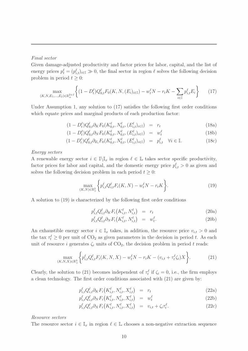
Final sector

Given damage-adjusted productivity and factor prices for labor, capital, and the list of

energy prices pℓt = (pℓi,t)i∈I ≫ 0, the final sector in region ℓ solves the following decision

problem in period t ≥ 0:

max(K,N,E1,...,EI)∈R

2+I+

{

(1−Dℓt)Q

ℓ0,tF0(K,N, (Ei)i∈I)− wℓ

tN − rtK −∑

i∈I

pℓi,tEi

}

(17)

Under Assumption 1, any solution to (17) satisfies the following first order conditions

which equate prices and marginal products of each production factor:

(1−Dℓt)Q

ℓ0,t∂KF0(K

ℓ0,t, N

ℓ0,t, (E

ℓi,t)i∈I) = rt (18a)

(1−Dℓt)Q

ℓ0,t∂NF0(K

ℓ0,t, N

ℓ0,t, (E

ℓi,t)i∈I) = wℓ

t (18b)

(1−Dℓt)Q

ℓ0,t∂Ei

F0(Kℓ0,t, N

ℓ0,t, (E

ℓi,t)i∈I) = pℓi,t ∀i ∈ I. (18c)

Energy sectors

A renewable energy sector i ∈ I\Ix in region ℓ ∈ L takes sector specific productivity,

factor prices for labor and capital, and the domestic energy price pℓi,t > 0 as given and

solves the following decision problem in each period t ≥ 0:

max(K,N)∈R2

+

{

pℓi,tQℓi,tFi(K,N)− wℓ

tN − rtK

}

. (19)

A solution to (19) is characterized by the following first order conditions

pℓi,tQℓi,t∂KFi

(Kℓ

i,t, Nℓi,t

)= rt (20a)

pℓi,tQℓi,t∂NFi

(Kℓ

i,t, Nℓi,t

)= wℓ

t . (20b)

An exhaustible energy sector i ∈ Ix takes, in addition, the resource price vi,t > 0 and

the tax τ ℓt ≥ 0 per unit of CO2 as given parameters in the decision in period t. As each

unit of resource i generates ζi units of CO2, the decision problem in period t reads:

max(K,N,X)∈R3

+

{

pℓi,tQℓi,tFi(K,N,X)− wℓ

tN − rtK − (vi,t + τ ℓt ζi)X

}

. (21)

Clearly, the solution to (21) becomes independent of τ ℓt if ζi = 0, i.e., the firm employs

a clean technology. The first order conditions associated with (21) are given by:

pℓi,tQℓi,t∂KFi

(Kℓ

i,t, Nℓi,t, X

ℓi,t

)= rt (22a)

pℓi,tQℓi,t∂NFi

(Kℓ

i,t, Nℓi,t, X

ℓi,t

)= wℓ

t (22b)

pℓi,tQℓi,t∂XFi

(Kℓ

i,t, Nℓi,t, X

ℓi,t

)= vi,t + ζiτ

ℓt . (22c)

Resource sectors

The resource sector i ∈ Ix in region ℓ ∈ L chooses a non-negative extraction sequence

10

(Xℓ,si,t )t≥0 which satisfies the resource constraint (4). Resources extracted in period t

are supplied to the global resource market. Given sequences of resource prices (vi,t)t≥0,

discount factors (qt)t≥0 defined by (12) and constant extraction costs ci ≥ 0, the resource

sector maximizes the discounted sum of future profits. The decision problem reads

max(Xℓ,s

i,t )t≥0

{ ∞∑

t=0

qt(vi,t − ci)Xℓ,si,t | X

ℓ,si,t ≥ 0 ∀t ≥ 0, (4) holds

}

. (23)

To avoid trivialities, assume Rℓi,0 > 0. Then, the existence of optimal extraction plans

determined as solutions to problem (23) can be characterized as follows.

Lemma 1

If Rℓi,0 > 0, the solution to (23) satisfies the following:

(i) An interior solution (X∗t )t≥0 ≫ 0 exists if and only if resource prices satisfy

vi,t − ci = (vi,0 − ci)/qt ≥ 0 ∀t ≥ 0. (24)

(ii) If condition (24) is satisfied, there are two cases:

(a) If vi,0 = ci, any sequence (X∗t )t≥0 satisfying

∑∞t=0 X

∗t ≤ Rℓ

i,0 is a solution.

(b) If vi,0 > ci, any sequence (X∗t )t≥0 satisfying

∑∞t=0 X

∗t = Rℓ

i,0 is a solution.

Condition (24) is a version of the classical Hotelling rule (cf. Hotelling (1931)) under

which net resource prices must grow at the rate of interest for resource firms to be

indifferent between extracting resources in different periods. Hassler & Krusell (2012)

also derive a version of the Hotelling rule in their multi-region framework. One also

observes from Lemma 1 (ii) that only in case (a) where vi,t = ci for all t ≥ 0 may it be

optimal not to exhaust the entire stock of resources.

In either case, (24) permits maximum profits Πℓi :=

∑∞t=0 qt(vi,t− ci)X

∗t to be written as

Πℓi = (vi,0 − ci)R

ℓi,0. (25)

Intuitively, the discounted profit stream (25) of resource sector i ∈ Ix is the excess value

of the initial stock of resources valued at time-zero prices net of extraction costs. Also

note that given an optimal extraction plan (Xℓ,si,t ) determined as a solution to (23), the

period profit of resource sector i ∈ Ix in region ℓ ∈ L is given by

Πℓi,t = (vi,t − ci)X

ℓ,si,t ≥ 0. (26)

In general, however, the quantity in (26) will be indeterminate at equilibrium due to

the multiplicity of solutions to (23).

Equilibrium profits

All firms in region ℓ are owned by domestic consumers who are entitled to receive all

11

profits. A direct consequence of Assumption 1 and the first order conditions derived in

(18), (20), and (22) is that profits in final production and all energy sectors are zero.

Thus, by (25) the total lifetime profit income of consumers in region ℓ ∈ L is

Πℓ =∑

i∈Ix

Πℓi =

∑

i∈Ix

(vi,0 − ci)Rℓi,0. (27)

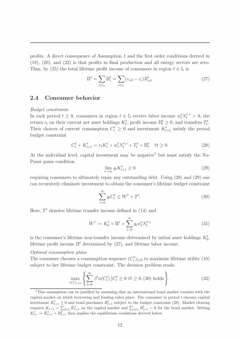
2.4 Consumer behavior

Budget constraints

In each period t ≥ 0, consumers in region ℓ ∈ L receive labor income wℓtN

ℓ,st > 0, the

return rt on their current net asset holdings Kℓt , profit income Πℓ

t ≥ 0, and transfers T ℓt .

Their choices of current consumption Cℓt ≥ 0 and investment Kℓ

t+1 satisfy the period

budget constraint

Cℓt +Kℓ

t+1 = rtKℓt + wℓ

tNℓ,st + T ℓ

t +Πℓt ∀t ≥ 0. (28)

At the individual level, capital investment may be negative7 but must satisfy the No-

Ponzi game condition

limt→∞

qtKℓt+1 ≥ 0 (29)

requiring consumers to ultimately repay any outstanding debt. Using (28) and (29) one

can recursively eliminate investment to obtain the consumer’s lifetime budget constraint

∞∑

t=0

qtCℓt ≤ W ℓ + T ℓ. (30)

Here, T ℓ denotes lifetime transfer income defined in (14) and

W ℓ := Kℓ0 +Πℓ +

∞∑

t=0

qtwℓtN

ℓ,st (31)

is the consumer’s lifetime non-transfer income determined by initial asset holdings Kℓ0,

lifetime profit income Πℓ determined by (27), and lifetime labor income.

Optimal consumption plans

The consumer chooses a consumption sequence (Cℓt )t≥0 to maximize lifetime utility (10)

subject to her lifetime budget constraint. The decision problem reads:

max(Cℓ

t )t≥0

{∞∑

t=0

βtu(Cℓt )∣∣Cℓ

t ≥ 0 ∀t ≥ 0, (30) holds

}

. (32)

7This assumption can be justified by assuming that an international bond market coexists with the

capital market on which borrowing and lending takes place. The consumer in period t chooses capital

investment Kℓt+1 ≥ 0 and bond purchases Bℓ

t+1 subject to the budget constraint (28). Market clearing

requires Kt+1 =∑

ℓ∈LKℓ

t+1 on the capital market and∑

ℓ∈LBℓ

t+1 = 0 for the bond market. Setting

Kℓt+ := Kℓ

t+1 +Bℓt+1 then implies the equilibrium conditions derived below.

12

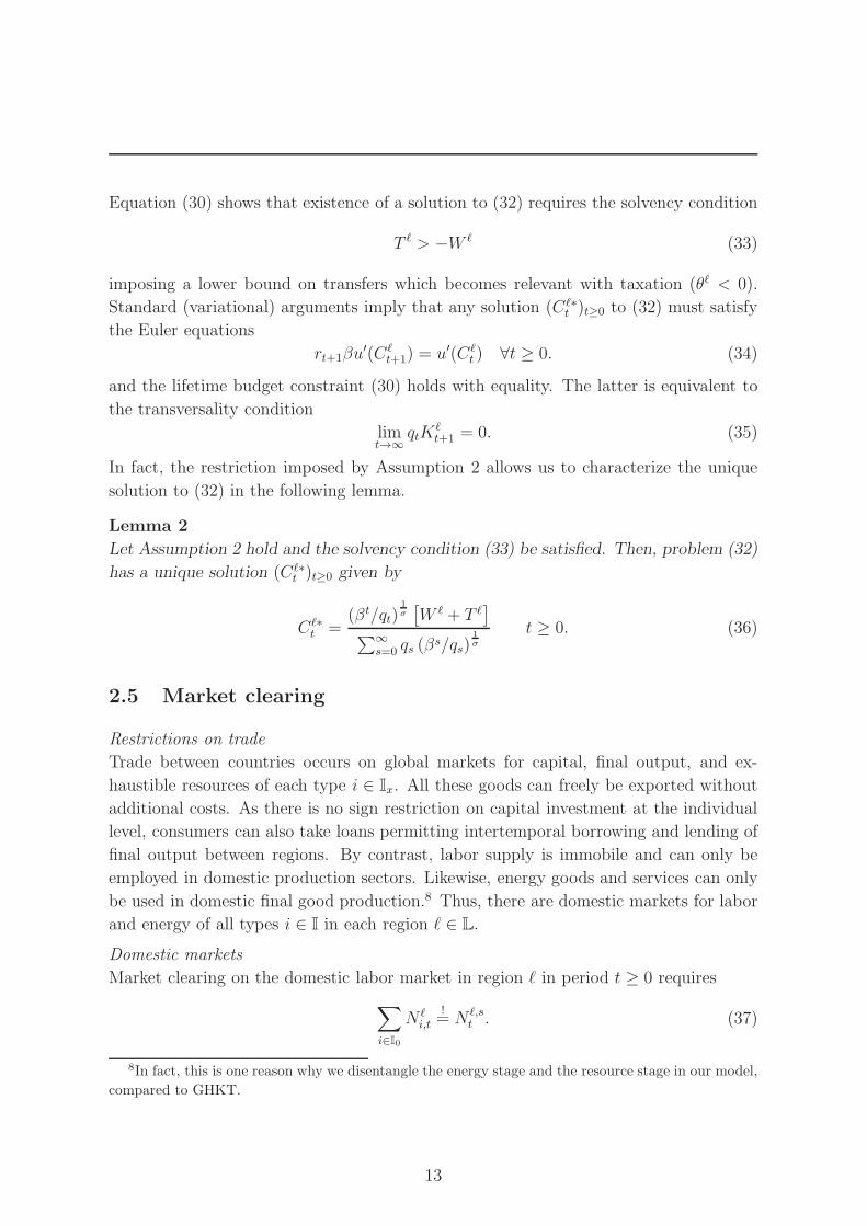
Equation (30) shows that existence of a solution to (32) requires the solvency condition

T ℓ > −W ℓ (33)

imposing a lower bound on transfers which becomes relevant with taxation (θℓ < 0).

Standard (variational) arguments imply that any solution (Cℓ∗t )t≥0 to (32) must satisfy

the Euler equations

rt+1βu′(Cℓ

t+1) = u′(Cℓt ) ∀t ≥ 0. (34)

and the lifetime budget constraint (30) holds with equality. The latter is equivalent to

the transversality condition

limt→∞

qtKℓt+1 = 0. (35)

In fact, the restriction imposed by Assumption 2 allows us to characterize the unique

solution to (32) in the following lemma.

Lemma 2

Let Assumption 2 hold and the solvency condition (33) be satisfied. Then, problem (32)

has a unique solution (Cℓ∗t )t≥0 given by

Cℓ∗t =

(βt/qt)1σ

[W ℓ + T ℓ

]

∑∞s=0 qs (β

s/qs)1σ

t ≥ 0. (36)

2.5 Market clearing

Restrictions on trade

Trade between countries occurs on global markets for capital, final output, and ex-

haustible resources of each type i ∈ Ix. All these goods can freely be exported without

additional costs. As there is no sign restriction on capital investment at the individual

level, consumers can also take loans permitting intertemporal borrowing and lending of

final output between regions. By contrast, labor supply is immobile and can only be

employed in domestic production sectors. Likewise, energy goods and services can only

be used in domestic final good production.8 Thus, there are domestic markets for labor

and energy of all types i ∈ I in each region ℓ ∈ L.

Domestic markets

Market clearing on the domestic labor market in region ℓ in period t ≥ 0 requires

∑

i∈I0

N ℓi,t

!= N ℓ,s

t . (37)

8In fact, this is one reason why we disentangle the energy stage and the resource stage in our model,

compared to GHKT.

13

Since energy is non-tradable across countries, energy demanded in final production must

coincide with domestic energy production in each region. The market clearing condition

for energy type i ∈ I in region ℓ ∈ L which must hold in each period t is therefore simply

Eℓi,t

!= Eℓ,s

i,t . (38)

International markets

Let Kt :=∑

ℓ∈L Kℓt be the aggregate stock of productive capital supplied to production

in period t. Market clearing on the world capital market in period t requires

∑

ℓ∈L

∑

i∈I0

Kℓi,t

!= Kt. (39)

Since period profit income (26) is, in general, indeterminate at equilibrium, so is con-

sumers’ individual net capital position Kℓt , ℓ ∈ L in the period budget constraint (28).

The market clearing condition for exhaustible resource i ∈ Ix in period t reads

∑

ℓ∈L

Xℓ,si,t

!=∑

ℓ∈L

Xℓi,t. (40)

If Xℓi,t < Xℓ,s

i,t region ℓ is a net exporter of resource i ∈ Ix in period t and a net importer

otherwise. Summing (4) over all countries and using (40), the allocation of resources

across production sectors must satisfy the world resource constraint

∞∑

t=0

∑

ℓ∈L

Xℓi,t ≤ Ri,0 (41)

where Ri,0 :=∑

ℓ∈L Rℓi,0 is the total initial stock of resource i. An immediate consequence

of Lemma 1 is that the equilibrium amount of resources Xℓ,si,t supplied by region ℓ and

period profits (26) will, in general, be indeterminate. As resources extracted in different

countries are perfect substitutes, however, the equilibrium extraction plans can always

be chosen compatible with the resource constraint (4) in each region.

Finally, summing the consumers’ period budget constraints (28) over all regions and

exploiting the first order and zero profit conditions for all sectors i ∈ I0 in conjunction

with (26) and the market clearing conditions (37), (38), (39), and (40) together with

(13) one obtains the market clearing condition for final output in period t as

Kt+1 +∑

ℓ∈L

Cℓt +

∑

i∈Ix

ci∑

ℓ∈L

Xℓi,t =

∑

ℓ∈L

Y ℓt . (42)

Here, Kt+1 is productive capital formed in period t and supplied to production in t+ 1.

14

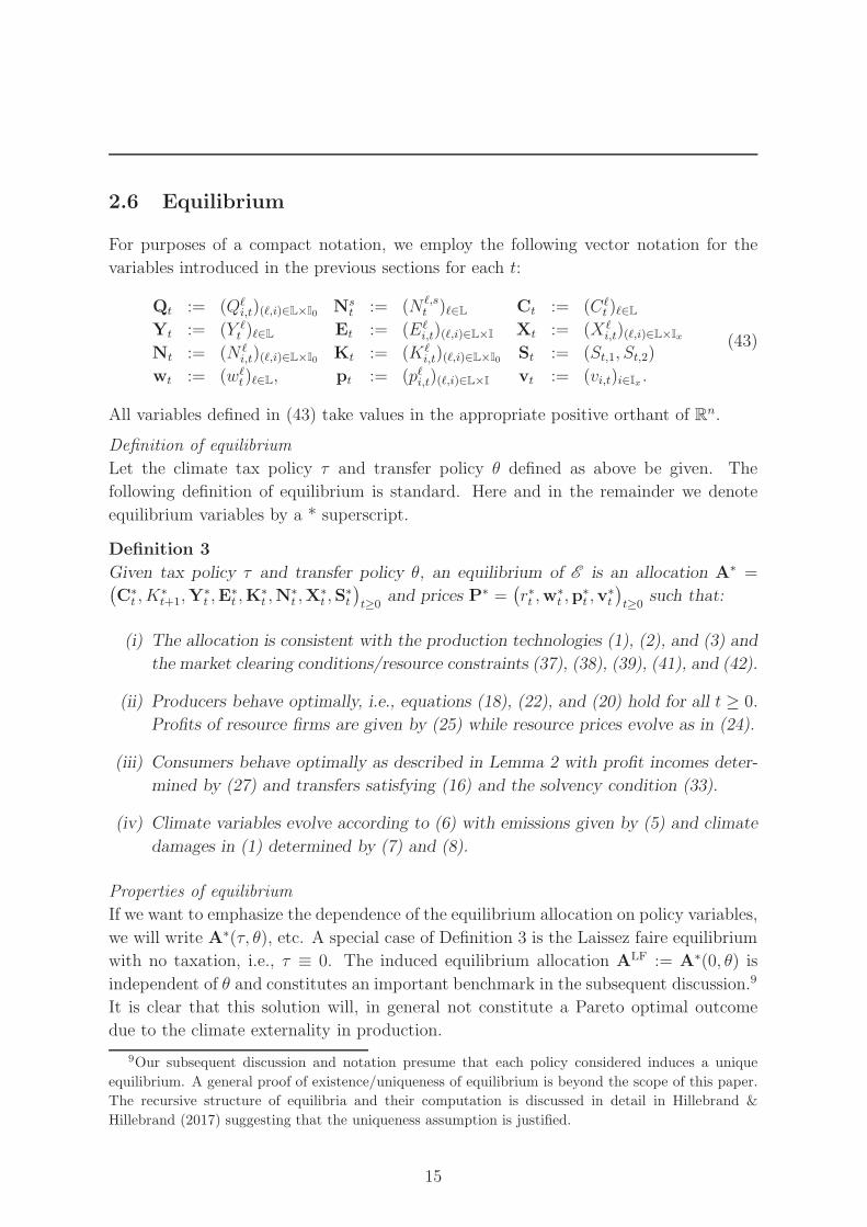
2.6 Equilibrium

For purposes of a compact notation, we employ the following vector notation for the

variables introduced in the previous sections for each t:

Qt := (Qℓi,t)(ℓ,i)∈L×I0

Nst := (N ℓ,s

t )ℓ∈L Ct := (Cℓt )ℓ∈L

Yt := (Y ℓt )ℓ∈L Et := (Eℓ

i,t)(ℓ,i)∈L×I Xt := (Xℓi,t)(ℓ,i)∈L×Ix

Nt := (N ℓi,t)(ℓ,i)∈L×I0

Kt := (Kℓi,t)(ℓ,i)∈L×I0

St := (St,1, St,2)

wt := (wℓt)ℓ∈L, pt := (pℓi,t)(ℓ,i)∈L×I vt := (vi,t)i∈Ix .

(43)

All variables defined in (43) take values in the appropriate positive orthant of Rn.

Definition of equilibrium

Let the climate tax policy τ and transfer policy θ defined as above be given. The

following definition of equilibrium is standard. Here and in the remainder we denote

equilibrium variables by a * superscript.

Definition 3

Given tax policy τ and transfer policy θ, an equilibrium of E is an allocation A∗ =(C∗

t , K∗t+1,Y

∗t ,E

∗t ,K

∗t ,N

∗t ,X

∗t ,S

∗t

)

t≥0and prices P∗ =

(r∗t ,w

∗t ,p

∗t ,v

∗t

)

t≥0such that:

(i) The allocation is consistent with the production technologies (1), (2), and (3) and

the market clearing conditions/resource constraints (37), (38), (39), (41), and (42).

(ii) Producers behave optimally, i.e., equations (18), (22), and (20) hold for all t ≥ 0.

Profits of resource firms are given by (25) while resource prices evolve as in (24).

(iii) Consumers behave optimally as described in Lemma 2 with profit incomes deter-

mined by (27) and transfers satisfying (16) and the solvency condition (33).

(iv) Climate variables evolve according to (6) with emissions given by (5) and climate

damages in (1) determined by (7) and (8).

Properties of equilibrium

If we want to emphasize the dependence of the equilibrium allocation on policy variables,

we will write A∗(τ, θ), etc. A special case of Definition 3 is the Laissez faire equilibrium

with no taxation, i.e., τ ≡ 0. The induced equilibrium allocation ALF := A∗(0, θ) is

independent of θ and constitutes an important benchmark in the subsequent discussion.9

It is clear that this solution will, in general not constitute a Pareto optimal outcome

due to the climate externality in production.

9Our subsequent discussion and notation presume that each policy considered induces a unique

equilibrium. A general proof of existence/uniqueness of equilibrium is beyond the scope of this paper.

The recursive structure of equilibria and their computation is discussed in detail in Hillebrand &

Hillebrand (2017) suggesting that the uniqueness assumption is justified.

15

The following results establish additional properties of equilibrium that follow from our

restrictions on technologies and preferences. As before, we denote by Ri,0 =∑

ℓ∈L Rℓi,0

to be the total initial stock of resource i ∈ Ix.

Lemma 3

Under Assumptions 1 and 2, any equilibrium allocation has the following properties:

(i) The allocation is interior, i.e., A∗ ≫ 0.

(ii) Consumption Cℓ∗t is a constant share of world consumption C∗

t :=∑

ℓ∈L Cℓ∗t , i.e.,

Cℓ∗t = µℓ∗C∗

t (44)

for all ℓ ∈ L and t ≥ 0 where µℓ∗ > 0 and∑

ℓ∈L µℓ∗ = 1.

(iii) Prices and extraction of each resource i ∈ Ix satisfy the following:

(a) If Ri,0 = ∞, then vi,0 = ci implying vi,t ≡ ci.

(b) If Ri,0 < ∞, then limt→∞(vi,t + ζiτℓt ) = ∞.

(c) If Ri,0 >∑∞

t=0

∑

ℓ∈L Xℓ∗i,t, then vi,0 = ci and limt→∞(vi,t + ζiτ

ℓt ) = ∞.

Lemma 3 (ii) shows that consumption in each region moves in lock-step with world con-

sumption over time. This property is due to consumer utility restricted by Assumption

2 and will play a key role to characterize how policy affects equilibrium allocations.

The result in (iii) shows that an infinite stock of resources drives resource prices down

to extraction costs. Hence, there is no scarcity rent on that resource and profits are

zero.10 Conversely, if the resource stock is finite, gross resource prices (including taxes)

must converge to infinity which requires vi,0 > ci in the absence of taxation. Moreover,

(iii) shows that each resource is completely exhausted unless its scarcity rent is zero

and taxes on emissions grow infinitely large. Thus, aggressive taxation is needed to

prevent resources from being completely exhausted. In particular, all resources are

fully exhausted at the Laissez faire equilibrium. See Hillebrand & Hillebrand (2017) for

further discussion and application of these results in a numerical study of the model.

The final result of this section disentangles the separate impact of the tax policy τ

and the transfer policy θ on the equilibrium allocation A∗(τ, θ). Essentially, it shows

that transfers only determine consumption in each region as a constant share of world

consumption but are irrelevant for all other equilibrium variables. This result will play

a major role in Section 4 when we study climate policies which implement the social

optimum as an equilibrium allocation.

10An infinite resource stock is typically justified by assuming the existence of a backstop technology

which provides an equivalent substitute for the resource in the future. Such a backstop technology is

implicitly assumed in GHKT for coal.Hillebrand & Hillebrand (2017) provide a critical discussion of

this asssumption and show that it is key to obtain the quantitative predictions in GHKT.

16

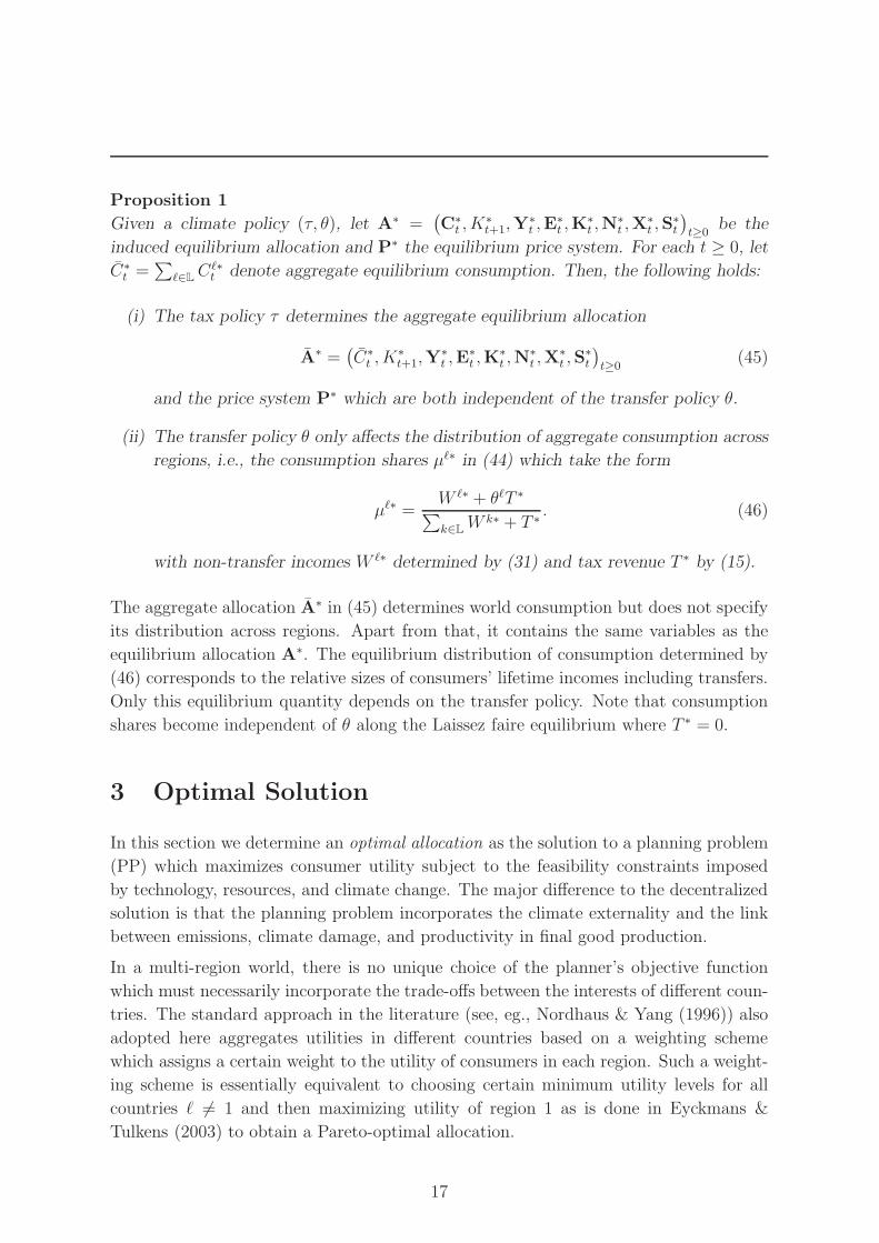
Proposition 1

Given a climate policy (τ, θ), let A∗ =(C∗

t , K∗t+1,Y

∗t ,E

∗t ,K

∗t ,N

∗t ,X

∗t ,S

∗t

)

t≥0be the

induced equilibrium allocation and P∗ the equilibrium price system. For each t ≥ 0, let

C∗t =

∑

ℓ∈L Cℓ∗t denote aggregate equilibrium consumption. Then, the following holds:

(i) The tax policy τ determines the aggregate equilibrium allocation

A∗ =(C∗

t , K∗t+1,Y

∗t ,E

∗t ,K

∗t ,N

∗t ,X

∗t ,S

∗t

)

t≥0(45)

and the price system P∗ which are both independent of the transfer policy θ.

(ii) The transfer policy θ only affects the distribution of aggregate consumption across

regions, i.e., the consumption shares µℓ∗ in (44) which take the form

µℓ∗ =W ℓ∗ + θℓT ∗

∑

k∈L Wk∗ + T ∗

. (46)

with non-transfer incomes W ℓ∗ determined by (31) and tax revenue T ∗ by (15).

The aggregate allocation A∗ in (45) determines world consumption but does not specify

its distribution across regions. Apart from that, it contains the same variables as the

equilibrium allocation A∗. The equilibrium distribution of consumption determined by

(46) corresponds to the relative sizes of consumers’ lifetime incomes including transfers.

Only this equilibrium quantity depends on the transfer policy. Note that consumption

shares become independent of θ along the Laissez faire equilibrium where T ∗ = 0.

3 Optimal Solution

In this section we determine an optimal allocation as the solution to a planning problem

(PP) which maximizes consumer utility subject to the feasibility constraints imposed

by technology, resources, and climate change. The major difference to the decentralized

solution is that the planning problem incorporates the climate externality and the link

between emissions, climate damage, and productivity in final good production.

In a multi-region world, there is no unique choice of the planner’s objective function

which must necessarily incorporate the trade-offs between the interests of different coun-

tries. The standard approach in the literature (see, eg., Nordhaus & Yang (1996)) also

adopted here aggregates utilities in different countries based on a weighting scheme

which assigns a certain weight to the utility of consumers in each region. Such a weight-

ing scheme is essentially equivalent to choosing certain minimum utility levels for all

countries ℓ 6= 1 and then maximizing utility of region 1 as is done in Eyckmans &

Tulkens (2003) to obtain a Pareto-optimal allocation.

17

A major advantage of our restrictions on preferences in Assumption 2 is that it per-

mits to compute an optimal allocation in two steps. First, we determine an efficient

allocation which maximizes utility of a fictitious world representative consumer. This

efficient solution completely specifies the optimal climate path and the entire alloca-

tion of production factors and resources across countries together with aggregate world

consumption. Most importantly, the efficient solution is independent of the employed

weighting scheme. In a second step, we determine an optimal distribution of world con-

sumption across different countries to obtain an optimal allocation which maximizes a

weighted utility index reflecting the trade-off between the interests of different coun-

tries. This separability between efficiency and optimal distribution will be the key to

determine an optimal climate policy in the next chapter.

3.1 Optimal allocations

Feasible allocations

Consider a planner who chooses a feasible world allocation subject to the restrictions

imposed by technology, factor mobility, and resource constraints. Formally, using the

notation introduced in the previous section, the planner takes the sequences of pro-

ductivity (Qt)t≥0 and labor supply (Nst)t≥0 as given. In addition, initial world capital

K0 > 0, the initial world stock Ri,0 > 0 of each exhaustible resource i ∈ Ix, and the

initial climate state S−1 = (S1,−1, S2,−1) are given as well. While final output, capi-

tal, and exhaustible resources can freely be allocated across countries, labor and energy

outputs can only be used within each region. Thus, the planner faces essentially the

same restrictions as producers and consumers in the decentralized solution including

constraints (37), (38), (39), and (42) when allocating labor, capital, and output. Fur-

ther, the given initial stock of world resources imposes the restrictions (41) on the use

of exhaustible resource i ∈ Ix in production.11 This leads to the following definition of

a feasible allocation.

Definition 4

(i) A feasible allocation is a sequence A =(Ct, Kt+1,Yt,Et,Kt,Nt,Xt,St

)

t≥0which

satisfies (1), (2), (3), (5), (6), (7), (37), (38), (39), (41), and (42) for all t ≥ 0.

(ii) The set of feasible allocations of the economy E is denoted A.

In particular, equilibrium allocations studied in the previous section are feasible, i.e.,

A∗ ∈ A.

11As resources extracted in different countries are perfect substitutes, the solution to the planning

problem does not determine where these resources are extracted. However, any allocation of exhaustible

resources (Xℓi,t)(ℓ,i)∈L×Ix

)t≥0 satisfying the feasibility constraint (41) can always be chosen compatible

with the individual resource constraints (4) in each region.

18

Objective function

The distribution of consumption across countries necessarily induces a trade-off between

the utility levels attained by consumers in different countries. To incorporate this trade-

off, assume that the planner uses a weighting scheme corresponding to a list of utility

weights ω = (ωℓ)ℓ∈L where ωℓ ≥ 0 represents the weight attached to consumer utility in

region ℓ in the planner’s decision. Formally, we have

Definition 5

A utility weighting scheme is a map ω : L −→ R+, ℓ 7→ ωℓ which satisfies∑

ℓ∈L ωℓ = 1.

In what follows, let ∆ := {(x1, . . . , xL) ∈ RL|∑L

ℓ=1 xℓ = 1} denote the unit-simplex in

RL. Then, the set of all possible weighting schemes can be identified with ∆+ := ∆∩RL

+.

Each weighting scheme ω ∈ ∆+ defines the following weighted utility index

V ((Ct)t≥0;ω) :=∞∑

t=0

βt∑

ℓ∈L

ωℓu(Cℓt ) (47)

which depends on world consumption (Ct)t≥0 where Ct = (Cℓt )ℓ∈L for all t ≥ 0.

Weighted Planning Problem

Given ω ∈ ∆+, use (47) to define the following Weighted Planning Problem (WPP)

maxA

{

V ((Ct)t≥0;ω)∣∣∣ A = (Ct, Kt+1,Yt,Et,Kt,Nt,Xt,St)t≥0 ∈ A

}

. (48)

Assuming it exists and is unique, denote the solution to (48) as

Aopt =(

Coptt , Kopt

t+1,Yoptt ,Eopt

t ,Koptt ,Nopt

t ,Xoptt ,Sopt

t )t≥0. (49)

It is clear that, in general, the solution to (48) will depend on the weighting scheme ω.

Thus, we will write Aopt(ω) as a way of emphasizing this dependence. It is also clear

that for any weighting scheme ω ∈ ∆+ the solution Aopt(ω) to (48) is a Pareto-optimum

on the set of feasible allocations A.

3.2 Efficient aggregate allocations

Feasible aggregate allocations

Consider now a modified planning problem which faces the same restrictions as before

but does not specify the distribution of consumption across different countries. As

before, denote aggregate world consumption in period t by Ct ≥ 0 and write the resource

constraint (42) as

Kt+1 + Ct +∑

ℓ∈L

∑

i∈Ix

ciXℓi,t =

∑

ℓ∈L

Y ℓt . (50)

Replacing (42) by (50) leads to the following definition of a feasible aggregate allocation

which specifies aggregate world consumption but not its distribution across countries.

Apart from that, it involves the same variables as a feasible allocation defined above.

19

Definition 6

(i) A feasible aggregate allocation is a sequence A =(Ct, Kt+1,Yt,Et,Kt,Nt,Xt,St

)

t≥0

which satisfies (1), (2), (3), (5), (6), (7), (37), (38), (39), (41), (50) for all t ≥ 0.

(ii) The set of feasible aggregate allocations of the economy E is denoted A.

In particular, the aggregate equilibrium allocation in (45) is feasible, i.e., A∗ ∈ A.

Aggregate planning problem

The modified planning problem maximizes utility of a fictitious world representative

consumer who consumes Ct in period t and has the same utility function as consumers

in each region. This leads to the following Aggregate Planning Problem (APP):

maxA

{ ∞∑

t=0

βtu(Ct)∣∣∣ A = (Ct, Kt+1,Yt,Et,Kt,Nt,Xt,St)t≥0 ∈ A

}

. (51)

A solution to (51) will be denoted

Aeff = (Cefft , Keff

t+1,Yefft ,Eeff

t ,Kefft ,Neff

t ,Xefft ,Seff

t )t≥0 (52)

and referred to as an efficient aggregate allocation. An efficient solution Aeff specifies

the entire allocation of production factors and resources across countries but leaves

undetermined the distribution of aggregate consumption across countries. It is therefore

independent of any weights attached to the interests of different countries and constitutes

the main ingredient to our separation result.

3.3 Optimal distribution of consumption

To prepare the main result of this section, let a weighting scheme ω ∈ ∆+ be arbitrary

but fixed and consider the static problem of distributing a given level C > 0 of aggre-

gate consumption across countries in an arbitrary period. The decision variable is a

consumption distribution µ = (µℓ)ℓ∈L where µℓ ≥ 0 is the share of C given to region

ℓ. Since∑

ℓ∈L µℓ = 1, any feasible consumption distribution satisfies µ ∈ ∆+ defined

as above. An optimal consumption distribution µopt = (µℓ,opt)ℓ∈L can be determined as

the solution to the problem

maxµ=(µℓ)ℓ∈L

{∑

ℓ∈L

ωℓu(µℓC)

∣∣∣∣µℓ ≥ 0 ∀ℓ ∈ L,

∑

ℓ∈L

µℓ ≤ 1

}

. (53)

The following lemma establishes that (53) has a unique solution which can be computed

explicitly and which, crucially, is independent of C. The result in (ii) establishes an

essential equivalence between the choice of a weighting scheme ω and a consumption

distribution µ which will be exploited in Section 4.3.

20

Lemma 4

Let u be of the form (11) from Assumption 2. Then, the following holds:

(i) For each weighting scheme ω = (ωℓ)ℓ∈L ∈ ∆+, there exists a unique consumption

distribution µopt(ω) = (µℓ,opt(ω))ℓ∈L which solves (53) taking the form

µℓ,opt(ω) =(ωℓ)

1σ

∑

k∈L(ωk)

1σ

, ℓ ∈ L. (54)

(ii) For any consumption distribution µ = (µℓ)ℓ∈L ∈ ∆+ there exists a weighting

scheme ω ∈ ∆+ which rationalizes µ in the sense that µ = µopt(ω) solves (53).

3.4 From efficiency to optimality

The main result of this section shows that the solution (49) to the WPP (48) can be

obtained from the efficient allocation (52) by distributing aggregate consumption opti-

mally across countries. Moreover, for any weighting scheme ω, the optimal distribution

is time-invariant and can be determined as the solution to (53). Using Lemma 4 allows

us to state this result in the following theorem.

Theorem 1

Let Assumptions 1 and 2 be satisfied and define the efficient allocation Aeff as in (52).

Given a weighting scheme ω, let µopt(ω) = (µℓ,opt(ω))ℓ∈L solve (53). Then, the allocation

A = (µopt(ω)Cefft , Keff

t+1,Yefft ,Eeff

t ,Kefft ,Neff

t ,Xefft ,Seff

t )t≥0 (55)

solves the WPP (48), i.e., A = Aopt(ω).

In words, Theorem 1 says that a solution to the WPP can simply be obtained from

the efficient solution (52) by distribution aggregate consumption in an optimal fashion

determined by the weighting scheme ω. In particular, the entire allocation of production

factors, resources, and emissions is completely determined by the efficient solution.

As its major implication, the previous result allows to compute a unique efficient allo-

cation of production factors, resources, emissions, climate damages, etc. which is com-

pletely independent of the weights that the interests of different countries receive in the

decision. The weighting scheme is therefore irrelevant for answering the question what

the optimal climate path is and where and how emissions should be reduced. Intuitively,

there exists a unique allocation of factors and resources across regions to produce an

efficient world consumption sequence which incorporates the climate externality. The

weighting scheme becomes relevant only to determine how this efficiently produced world

consumption sequence should be distributed across regions. An optimal consumption

distribution can be computed using (54) once a suitable weighting scheme has been

chosen and, by Lemma 4 (ii) is in fact equivalent to such a choice.

21

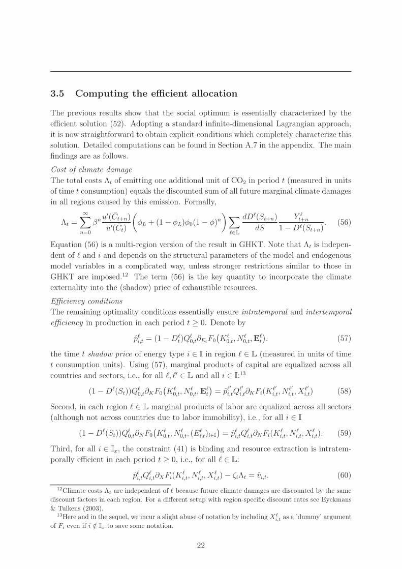
3.5 Computing the efficient allocation

The previous results show that the social optimum is essentially characterized by the

efficient solution (52). Adopting a standard infinite-dimensional Lagrangian approach,

it is now straightforward to obtain explicit conditions which completely characterize this

solution. Detailed computations can be found in Section A.7 in the appendix. The main

findings are as follows.

Cost of climate damage

The total costs Λt of emitting one additional unit of CO2 in period t (measured in units

of time t consumption) equals the discounted sum of all future marginal climate damages

in all regions caused by this emission. Formally,

Λt =∞∑

n=0

βnu′(Ct+n)

u′(Ct)

(

φL + (1− φL)φ0(1− φ)n)∑

ℓ∈L

dDℓ(St+n)

dS

Y ℓt+n

1−Dℓ(St+n). (56)

Equation (56) is a multi-region version of the result in GHKT. Note that Λt is indepen-

dent of ℓ and i and depends on the structural parameters of the model and endogenous

model variables in a complicated way, unless stronger restrictions similar to those in

GHKT are imposed.12 The term (56) is the key quantity to incorporate the climate

externality into the (shadow) price of exhaustible resources.

Efficiency conditions

The remaining optimality conditions essentially ensure intratemporal and intertemporal

efficiency in production in each period t ≥ 0. Denote by

pℓi,t = (1−Dℓt)Q

ℓ0,t∂Ei

F0

(Kℓ

0,t, Nℓ0,t,E

ℓt

). (57)

the time t shadow price of energy type i ∈ I in region ℓ ∈ L (measured in units of time

t consumption units). Using (57), marginal products of capital are equalized across all

countries and sectors, i.e., for all ℓ, ℓ′ ∈ L and all i ∈ I:13

(1−Dℓ(St))Qℓ0,t∂KF0

(Kℓ

0,t, Nℓ0,t,E

ℓt

)= pℓ

′

i,tQℓ′

i,t∂KFi(Kℓ′

i,t, Nℓ′

i,t, Xℓ′

i,t) (58)

Second, in each region ℓ ∈ L marginal products of labor are equalized across all sectors

(although not across countries due to labor immobility), i.e., for all i ∈ I

(1−Dℓ(St))Qℓ0,t∂NF0

(Kℓ

0,t, Nℓ0,t, (E

ℓi,t)i∈I

)= pℓi,tQ

ℓi,t∂NFi(K

ℓi,t, N

ℓi,t, X

ℓi,t). (59)

Third, for all i ∈ Ix, the constraint (41) is binding and resource extraction is intratem-

porally efficient in each period t ≥ 0, i.e., for all ℓ ∈ L:

pℓi,tQℓi,t∂XFi(K

ℓi,t, N

ℓi,t, X

ℓi,t)− ζiΛt = vi,t. (60)

12Climate costs Λt are independent of ℓ because future climate damages are discounted by the same

discount factors in each region. For a different setup with region-specific discount rates see Eyckmans

& Tulkens (2003).13Here and in the sequel, we incur a slight abuse of notation by including Xℓ

i,t as a ’dummy’ argument

of Fi even if i /∈ Ix to save some notation.

22

Equation (60) defines the true shadow price of resources as the marginal product in

production minus the cost of emissions defined in (56). Compared to the laissez-faire

equilibrium allocation, the social planner includes a wedge between the marginal product

of dirty resource i and its (shadow) price which accounts for the externality cost of an

additional unit of emissions. This is the key difference to the equilibrium condition (22c)

along the Laissez faire equilibrium which fails to take this cost into account. If Dℓ ≡ 0,

however, the efficient solution coincides with the aggregate equilibrium allocation (45).

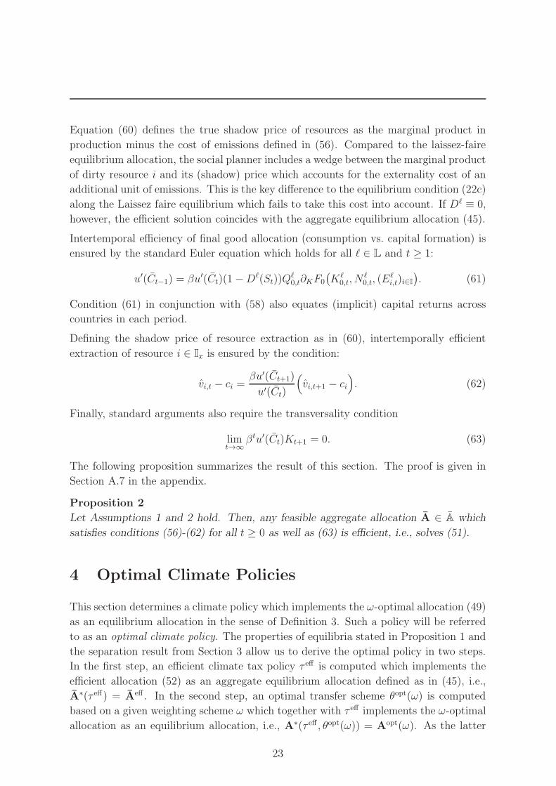
Intertemporal efficiency of final good allocation (consumption vs. capital formation) is

ensured by the standard Euler equation which holds for all ℓ ∈ L and t ≥ 1:

u′(Ct−1) = βu′(Ct)(1−Dℓ(St))Qℓ0,t∂KF0

(Kℓ

0,t, Nℓ0,t, (E

ℓi,t)i∈I

). (61)

Condition (61) in conjunction with (58) also equates (implicit) capital returns across

countries in each period.

Defining the shadow price of resource extraction as in (60), intertemporally efficient

extraction of resource i ∈ Ix is ensured by the condition:

vi,t − ci =βu′(Ct+1)

u′(Ct)

(

vi,t+1 − ci

)

. (62)

Finally, standard arguments also require the transversality condition

limt→∞

βtu′(Ct)Kt+1 = 0. (63)

The following proposition summarizes the result of this section. The proof is given in

Section A.7 in the appendix.

Proposition 2

Let Assumptions 1 and 2 hold. Then, any feasible aggregate allocation A ∈ A which

satisfies conditions (56)-(62) for all t ≥ 0 as well as (63) is efficient, i.e., solves (51).

4 Optimal Climate Policies

This section determines a climate policy which implements the ω-optimal allocation (49)

as an equilibrium allocation in the sense of Definition 3. Such a policy will be referred

to as an optimal climate policy. The properties of equilibria stated in Proposition 1 and

the separation result from Section 3 allow us to derive the optimal policy in two steps.

In the first step, an efficient climate tax policy τ eff is computed which implements the

efficient allocation (52) as an aggregate equilibrium allocation defined as in (45), i.e.,

A∗(τ eff) = Aeff . In the second step, an optimal transfer scheme θopt(ω) is computed

based on a given weighting scheme ω which together with τ eff implements the ω-optimal

allocation as an equilibrium allocation, i.e., A∗(τ eff , θopt(ω)) = Aopt(ω). As the latter

23

requires the choice of a weighting scheme ω, we offer a simple idea how such a scheme

could be chosen such that each region has an incentive to adopt the optimal climate tax

policy.

4.1 The optimal climate tax policy

Using the efficient allocation (52), define the climate tax policy τ eff = (τ efft )t≥0 as

τ efft =

∞∑

n=0

βnu′(Ceff

t+n)

u′(Cefft )

(

φL + (1− φL)φ0(1− φ)n)∑

ℓ∈L

dDℓ(Sefft+n)

dS

Y ℓ,efft+n

1−Dℓ(Sefft+n)

, t ≥ 0.

(64)

Equation (64) is a classical example of a Pigovian tax which equates taxes to the total

discounted marginal damage caused by each unit of CO2 determined by (56). Under

this policy, emissions taxes τ ℓt ≡ τ efft are uniform across dirty sectors in all countries and

incorporate the total damage from emitting one unit of CO2 in period t. The following

result shows that this policy implements the efficient solution (52) as an aggregate

equilibrium allocation defined as in (45). Recall from Proposition 1 that this allocation

is independent of the transfer policy. Thus, the CTP defined by (64) will be referred to

as the efficient tax policy.

Theorem 2

Let Assumptions 1 and 2 hold and define the climate tax policy τ eff as in (64). Then, the

induced aggregate equilibrium allocation defined in (45) is efficient, i.e., A∗(τ eff) = Aeff .

With the specific functional forms (9) and (11) for climate damage and consumer utility,

the efficient tax formula (64) takes the more specific form

τ efft =

∞∑

n=0

βn

(Ceff

t+n

Cefft

)−σ (

φL + (1− φL)φ0(1− φ)n)∑

ℓ∈L

γℓY ℓ,efft+n . (65)

In particular, efficient taxes are zero if climate damages are absent, i.e., γℓ ≡ 0.

In general, expression (65) can not be computed explicitly, as it involves the entire paths

of future output in each region and aggregate consumption. However, if the efficient

solution induces a balanced growth path on which output and consumption grow at

constant and identical rate g ≥ 0, (65) takes the much simpler form

τ efft = τ eff∑

ℓ∈L

γℓY ℓ,efft , τ eff :=

φL

1− β(1 + g)1−σ+ φ0

1− φL

1− β(1 + g)1−σ(1− φ). (66)

Thus, on a balanced growth path, the optimal tax is a constant share τ eff of world output

weighted by the damage parameters γℓ. For logarithmic utility (σ = 1) and homogeneous

climate damages (γℓ ≡ γ), equation (66) recovers precisely the tax-formula derived in

24

GHKT under a set of additional restrictions (log utility, Cobb-Douglas production,

all capital used in the final sector). None of these restrictions is required here if the

assumption of a balanced growth path is satisfied. Numerical simulations of the model

presented in Hillebrand & Hillebrand (2017) show that the efficient solution converges

quickly to a balanced growth path suggesting that (65) is well-approximated by (66) in

applications of the model.

4.2 Optimal transfer policies

Under the efficient climate tax policy (64), the aggregate equilibrium allocation (45)

coincides with the efficient allocation (52). While this determines aggregate world con-

sumption together with an optimal allocation of production factors and climate variables

in each period, it leaves undetermined how world consumption is distributed across coun-

tries. The latter requires the choice of a weighting scheme ω ∈ ∆+ based on which the

optimal consumption distribution µopt(ω) can be determined by (53).

We now explore the existence of a transfer policy θ under which the induced equilibrium

allocation A∗(τ eff , θ) coincides with the optimal allocation Aopt(ω) defined in (49) in

which each region attains the optimal consumption share µopt(ω). As before, let τ eff be

the efficient tax policy which implements the efficient aggregate allocation Aeff and, by

Lemma 3 also determines the price system Peff supporting the efficient allocation. Let

W ℓ,eff denote the induced lifetime non-transfer income of consumers in region ℓ defined

in (31), W eff :=∑

ℓ∈L Wℓ,eff aggregate non-transfer lifetime income and T eff the total

tax revenue defined as in (15). Given a weighting scheme ω ∈ ∆+ and consumption

shares µopt(ω) = (µℓ,opt(ω))ℓ∈L determined by Lemma 4, consider the following transfer

policy θopt = (θℓ,opt)ℓ∈L defined for each ℓ ∈ L as

θℓ,opt(ω) =µℓ,opt(ω)

(W eff + T eff

)−W ℓ,eff

T eff. (67)

Note that (67) determines consumer ℓ’s lifetime cum-transfer income W ℓ + T ℓ to be a

share µℓ,opt(ω) of world cum-transfer income W eff+T eff . The following result shows that

the transfer policy (67) together with τ eff constitutes indeed an optimal climate policy.

Theorem 3

Let Assumptions 1 and 2 hold and define the climate tax policy τ eff as in (64). Given any

weighting scheme ω ∈ ∆+, define µopt(ω) by (53) and the transfer policy θopt(ω) by (67).

Then, the induced equilibrium allocation is ω-optimal, i.e., A∗(τ eff , θopt(ω)) = Aopt(ω).

4.3 A Pareto-improving transfer policy

Applying the optimal transfer policy defined in (67) requires the choice of a particular

weighting scheme ω ∈ ∆+ or, equivalently, invoking Lemma 4 (ii), a desired consumption

25

distribution µ = (µℓ)ℓ∈L ∈ ∆+. This raises the question how such a distribution can

and should be determined. Ideally, one might want to choose ω resp. µ as an equal

weighting scheme based, e.g., on relative population sizes to ensure a fair world allocation

of consumption. In any quantitative study of the model, however, such a choice would

induce massive transfers unrelated to climate change but due to the fact that the world

income distribution is very unequal and strongly biased towards industrialized countries.

The analysis of this paper, however, is not about fairness and redistribution of world

income but how transfers can be determined such that each region has an incentive to

implement the optimal tax on emissions. For this reason, the present section offers an

alternative approach which chooses the consumption distribution based on the shares

that each region attains in the Laissez faire allocation. This target seems a natural choice

because the Laissez faire solution corresponds to the extreme case where all countries

agree not to take any measures against climate change. It is therefore a natural threat

point in any bargaining process about transfers.

Formally, let µLF = (µℓ,LF)ℓ∈L denote the consumption shares along the Laissez faire

equilibrium allocationALF which are constant by Lemma 3 (ii). Using the same notation

as in the previous subsection, define the transfer policy θLF = (θℓ,LF)ℓ∈L ∈ ∆ as

θℓ,LF :=µℓ,LF

(W eff + T eff

)−W ℓ,eff

T eff, ℓ ∈ L. (68)

Under transfer policy θLF, each region ℓ attains the same relative wealth and the same

share µℓ,LF of world consumption along the efficient equilibrium allocation as in the

Laissez faire allocation. The following main result shows that this policy makes each

country better-off, i.e., consumers in each region enjoy utility strictly higher than in the

Laissez faire allocation if they agree to jointly implement the efficient tax policy.14

Theorem 4

The equilibrium allocation A∗(τ eff , θLF) Pareto-improves the laissez faire allocationALF.

4.4 Emissions trading systems

Instead of levying a tax on emissions, an alternative policy to curb emissions is to intro-

duce a global emissions trading system (ETS). Such a system issues a certain number

of emission allowances in each period which put an upper bound on Carbon emissions

in that period. The possession of one emission allowance for period t allows the owner

to emit one unit of fossil energy/carbon dioxide into the atmosphere in that period. For

simplicity, assume that allowances are time-specific, i.e., can not be transferred across

14Clearly, this does not eliminate the free-riding problem that a single region may have an incentive

to deviate from the optimal policy. A more elaborate game-theoretic analysis of this problem within

the previous framework is beyond the scope of this paper but left for future research.

26

different periods. Then, the total number of allowances issued in period t puts an upper

bound (’cap’) on CO2 emissions in that period. For this reason, an emissions-trading

system is also called a ’cap-and trade system’. As the equilibrium effects of an emissions

trading system are independent of the distribution of emission rights across sectors or

regions, such a system can formally be defined a follows.

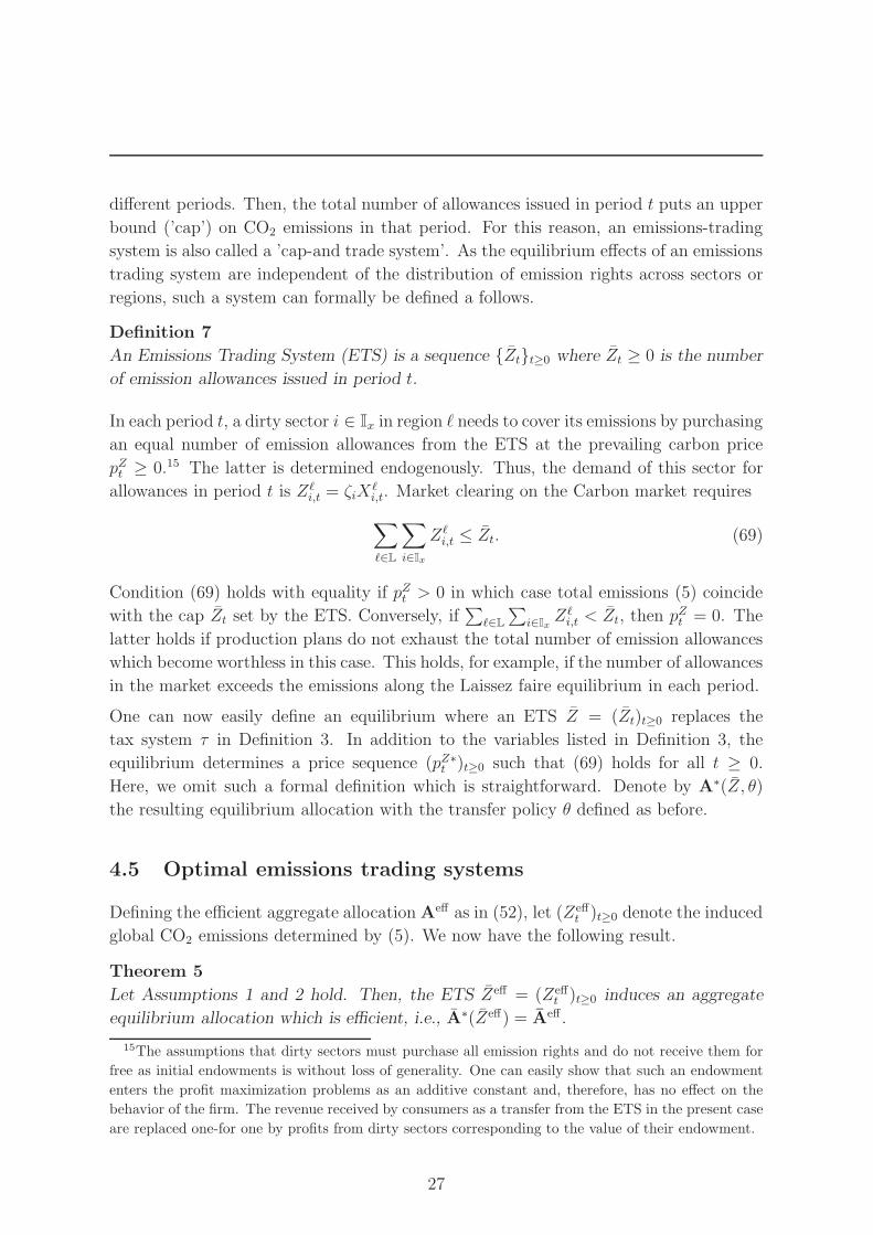
Definition 7

An Emissions Trading System (ETS) is a sequence {Zt}t≥0 where Zt ≥ 0 is the number

of emission allowances issued in period t.

In each period t, a dirty sector i ∈ Ix in region ℓ needs to cover its emissions by purchasing

an equal number of emission allowances from the ETS at the prevailing carbon price

pZt ≥ 0.15 The latter is determined endogenously. Thus, the demand of this sector for

allowances in period t is Zℓi,t = ζiX

ℓi,t. Market clearing on the Carbon market requires

∑

ℓ∈L

∑

i∈Ix

Zℓi,t ≤ Zt. (69)

Condition (69) holds with equality if pZt > 0 in which case total emissions (5) coincide

with the cap Zt set by the ETS. Conversely, if∑

ℓ∈L

∑

i∈IxZℓ

i,t < Zt, then pZt = 0. The

latter holds if production plans do not exhaust the total number of emission allowances

which become worthless in this case. This holds, for example, if the number of allowances

in the market exceeds the emissions along the Laissez faire equilibrium in each period.

One can now easily define an equilibrium where an ETS Z = (Zt)t≥0 replaces the

tax system τ in Definition 3. In addition to the variables listed in Definition 3, the

equilibrium determines a price sequence (pZ∗t )t≥0 such that (69) holds for all t ≥ 0.

Here, we omit such a formal definition which is straightforward. Denote by A∗(Z, θ)

the resulting equilibrium allocation with the transfer policy θ defined as before.

4.5 Optimal emissions trading systems

Defining the efficient aggregate allocationAeff as in (52), let (Zefft )t≥0 denote the induced

global CO2 emissions determined by (5). We now have the following result.

Theorem 5

Let Assumptions 1 and 2 hold. Then, the ETS Zeff = (Zefft )t≥0 induces an aggregate

equilibrium allocation which is efficient, i.e., A∗(Zeff) = Aeff .

15The assumptions that dirty sectors must purchase all emission rights and do not receive them for

free as initial endowments is without loss of generality. One can easily show that such an endowment

enters the profit maximization problems as an additive constant and, therefore, has no effect on the

behavior of the firm. The revenue received by consumers as a transfer from the ETS in the present case

are replaced one-for one by profits from dirty sectors corresponding to the value of their endowment.

27

The previous result shows that the efficient allocation can be implemented by issuing

emission allowances (’caps’) equal to the optimal emissions path determined by the

efficient allocation. Further, the equilibrium Carbon price sequence (pZ∗t )t≥0 coincides

with the optimal tax defined in (56). Hence, we can directly interpret this tax as the

price for CO2. Given a weighting scheme ω ∈ ∆+, one can define the transfer policy as

in (67) to obtain an equilibrium allocation A∗(Zeff , θopt) which is ω-optimal. Here, the

transfer policy would distribute the revenue from auctioning the emission allowances in

each period across countries.

5 Conclusions

The problem of determining an optimal climate path and an efficient allocation of pro-

duction factors and exhaustible resources admits a unique solution which is completely

independent of the interests of different countries. This solution can be implemented as a

decentralized equilibrium by levying a uniform global tax on carbon emission which can

be computed (or approximated) in closed form. Alternatively, this can be achieved by

a globally organized emissions trading system where the ’caps’ are uniquely determined

by the efficient climate path. In principle, all countries should agree on this policy.

The real issue in the political debate about climate change is therefore not how and

where emissions should be taxed, but rather how countries should share the tax revenue

via transfers. These transfers determine the world distribution of consumption or income

and provide a mechanism to compensate regions for climate damages. As the choice of

an optimal transfer policy induces a trade-off between the interests of different countries,

one might want to determine the transfer policy such that each region has an incentive

to implement the optimal tax policy. An example of a transfer policy which leads to a

Pareto-improvement relative to the Laissez faire allocation was devised in this paper.

The latter result is only a first step towards a more elaborate model of the political

process which determines climate policies. In future research, we intend to model this

process as a (cooperative or non-cooperative) game between regions as in Dutta &

Radner (2006). Within the framework of this paper, L would be the set of players each

of which chooses a domestic emissions tax policy τ ℓ as their strategy and receives utility

of domestic consumers as their pay-off. Transfers across regions then correspond to side

payments which can be used to incentivize each region to implement a certain strategy.

This raises the question whether there exists a transfer policy under which the optimal

climate tax policy derived in this paper can be obtained as the Nash equilibrium of this

non-cooperative game. In addition, one could also look a cooperative versions of this

game where regions join forces to combat climate change by forming coalitions.

In addition, the framework developed in this paper can be extended in various directions.

One such extensions is to replace the deterministic setup by a stochastic environment

28

with random perturbations which allows to include various forms of uncertainty into the

model. A second extension is a setup with endogenous growth and directed technical

change as in Acemoglu, Aghion, Bursztyn & Hemous (2012). Both modifications were

considered in GHKT and we believe that our framework is also amendable to them.

A Mathematical Appendix

A.1 Proof of Lemma 1

Using standard Lagrangian arguments, a non-negative sequence (X∗t )t≥0 is a solution to

(23) if∑∞

t=0X∗t ≤ Rℓ

i,0 and there exist non-negative Lagrangian variables (σ∗t )t≥0 and

µ ≥ 0 such that ((X∗t , σ

∗t )t≥0, µ) solve

qt(vi,t − ci) + σt − µ = 0 ∀t ≥ 0 (A.1a)

σtXt = 0 ∀t ≥ 0 (A.1b)

µ( ∞∑

t=0

Xt − Rℓi,0

)

= 0. (A.1c)

If X∗t > 0 for all t ≥ 0, then, σt = 0 by (A.1b) and vi,t ≥ ci by (A.1a) for all t. Using

q0 = 1 and qt/qt−1 = r−1t for all t > 0 in (A.1a), resource prices must evolve as in (24).

The remaining assertions follow immediately. �

A.2 Proof of Lemma 2

Under Assumption 2, (12) and (34) imply that the solution to (32) evolves as

Cℓ∗t = Cℓ∗

t−1(βrt)1σ = Cℓ∗

0

t∏

s=1

(βrs)1σ = Cℓ∗

0

(βt

qt

) 1σ

t ≥ 1. (A.2)

Using (A.2), the l.h.s. in the lifetime budget constraint (30) can be written as

∞∑

t=0

qtCℓ∗t =

∞∑

t=0

qtCℓ∗0

(βt/qt

) 1σ = Cℓ∗

0

∞∑

t=0

(βtqσ−1

t

) 1σ . (A.3)

Using (A.3) in (30) - which holds with equality- gives

Cℓ∗0 =

W ℓ + T ℓ

∑∞t=0

(βtqσ−1

t

) 1σ

. (A.4)

Using (A.4) in (A.2) yields (36). �

29

A.3 Proof of Lemma 3

(i) This is a direct consequence of the equilibrium conditions (18), (20), (22) and the

boundary behavior of Fi and u imposed by Assumptions 1 and 2.

(ii) Set µℓ∗ := Cℓ∗0 /C∗

0 for ℓ ∈ L. By Lemma 2, the growth rates of each sequence

(Cℓ∗t )t≥0 are independent of ℓ and equal to the growth rates of aggregate consumption

(C∗t )t≥0. Induction then implies that (44) holds for all t ≥ 0.

(iii) Let i ∈ Ix be arbitrary. If Ri,0 = ∞, there exists a region ℓ ∈ L for which Rℓi,0 = ∞.

As profits must be finite at equilibrium, (25) implies vi,0 − ci.

If Ri,0 < ∞, (41) implies limt→∞Xℓi,t = 0 for all ℓ ∈ L. The boundary behavior from

Assumption 1 gives limt→∞ ∂XFi

(Kℓ

i,t, Nℓi,t, X

ℓi,t

)= ∞ and the claim therefore follows

from (22c).

If Ri,0 >∑∞

t=0

∑

ℓ∈L Xℓ∗i,t, the same arguments employed to prove (b) give the second

result while the first one follows from Lemma 1 (ii). �

A.4 Proof of Proposition 1

(i) Using the result from Lemma 2, aggregate consumption in period t satisfies

C∗t =

(βt/qt)1σ

[∑

ℓ∈L Wℓ + T

]

∑∞s=0 qs (β

s/qs)1σ

t ≥ 0 (A.5)

and determines Kt+1 by (42). These and all other equations relevant to determine the

variables in A∗ and prices P∗ are independent of θ.

(ii) Using Lemma 2 and (14) in conjunction with (46) and (A.5) gives

Cℓ∗t =

(βt/qt)1σ

[W ℓ + θℓT

]

∑∞s=0 qs (β

s/qs)1σ

= µℓ∗C∗t

for all t ≥ 0 and ℓ ∈ L, proving the claim. �

A.5 Proof of Lemma 4

(i) Let ω ∈ ∆+ and C > 0 be given. It is clear that ωℓ = 0 implies µℓ = 0 which is

implied by the solution (54). As we can always restate problem (54) as a maximization

problem involving only those µℓ for which ωℓ > 0, the remainder of the proof assumes

w.l.o.g. that ω ≫ 0. The boundary behavior of u defined in (11) implies that any

solution to (53) is bounded away from zero by, say, µ = (µℓ)ℓ∈L ≫ 0. This and the

constraint∑

ℓ∈L µℓ ≤ 1 define a compact, convex subset of R

L++ on which the map

µ 7→∑

ℓ∈L ωℓu(µℓ) is continuous and strictly concave ensuring that (53) has a unique

30

solution µopt. Standard Lagrangian type arguments imply the existence of a multiplier

λ > 0 such that the solution satisfies µℓ = (ωℓC1−σ/λ)1σ for all ℓ ∈ L and

∑

ℓ∈L µℓ = 1.

Combining these conditions to eliminate C1−σ/λ gives (54). For later reference, let a = 0

if σ 6= 1 and a = 1 otherwise and use (11) to write the objective function in (53) as

∑

ℓ∈L

ωℓu(µℓC) = a

(

u(C) +∑

ℓ∈L

ωℓu(µℓ)

)

+ (1− σ) u(C)∑

ℓ∈L

ωℓu(µℓ). (A.6)

Using (A.6), the maximum value (53) can be expressed as

∑

ℓ∈L

ωℓu(µℓ,optC) =

{(1− σ)m(ω)u(C) σ 6= 1

m(ω) + u(C) σ = 1(A.7)

where m(ω) :=∑

ℓ∈L ωℓu(µℓ,opt(ω)). Note that (1− σ)m(ω) > 0 whenever σ 6= 1.

(ii) Let µ = (µℓ)ℓ∈L ∈ ∆+ be arbitrary. Defining ωℓ := (µℓ)σ(∑

k∈L(µk)σ)−1 for each

ℓ ∈ L, one verifies directly that µ = µopt(ω) solves (53) under this weighting scheme. �

A.6 Proof of Theorem 1

Let a weighting scheme ω ∈ ∆+ be arbitrary but fixed and µopt(ω) be the unique solution

to (53). Denote the efficient solution (52) to the APP (51) by Aeff = (Cefft ,Γeff

t )t≥0 ∈ A

and define A = (Ct,Γefft )t≥0 ∈ A where Ct = (Cℓ

t )ℓ∈L := µopt(ω)Cefft as in the theorem.

To establish that A is ω-optimal, i.e., solves (48), let A′ = (C′t,Γ

′t)t≥0 ∈ A be any other

feasible allocation where C′t = (Cℓ′

t )ℓ∈L, t ≥ 0. We have to show that

V ((C′t)t≥0;ω) ≤ V ((Ct)t≥0;ω). (A.8)

Define aggregate consumption (C ′t)t≥0 induced by (C′

t)t≥0 as C ′t :=

∑

ℓ∈L Cℓ′

t , t ≥ 0.

Then, (C ′t,Γ

′t)t≥0 ∈ A and, since (Ceff

t ,Γefft )t≥0 solves the APP (51),

∞∑

t=0

βtu(C ′t) ≤

∞∑

t=0

βtu(Cefft ). (A.9)

Let a = 1 if σ = 1 and a = 0 otherwise. By (53) and (A.7), we have for all t ≥ 0

∑

ℓ∈L

ωℓu(Cℓ′

t ) ≤∑

ℓ∈L

ωℓu(µℓ,opt(ω)C ′t) = a

(m(ω) + u(C ′

t))+ (1− σ)m(ω)u(C ′

t) (A.10)

and

∑

ℓ∈L

ωℓu(Cℓt ) =

∑

ℓ∈L

ωℓu(µℓ,opt(ω)Cefft ) = a

(

m(ω)+u(Cefft ))

+(1−σ)m(ω)u(Cefft ). (A.11)

31

Equations (A.10) and (A.11) being true for all t ≥ 0 and (A.9) then give

V ((C′t)t≥0;ω) =

∞∑

t=0

βt∑

ℓ∈L

ωℓu(Cℓ′

t )

≤ a

(

m(ω)

1− β+

∞∑

t=0

βtu(C ′t)

)

+ (1− σ)m(ω)

∞∑

t=0

βtu(C ′t)

≤ a

(

m(ω)

1− β+

∞∑

t=0

βtu(Cefft )

)

+ (1− σ)m(ω)

∞∑

t=0

βtu(Cefft )

=

∞∑

t=0

βt∑

ℓ∈L

ωℓu(Cℓt ) = V ((Ct)t≥0;ω)

This proves (A.8) and the claim. �

A.7 Computing the efficient solution (52)

We adopt a standard Langrangian approach also used in GHKT to characterize the

solution (52). For brevity, use (43) setting Eℓt := (Eℓ

i,t)i∈I, Dℓt := Dℓ(S1,t + S2,t). Define

Lagrangen multipliers λt := (λ0,t, ((λℓi,t)i∈I0 , λ

ℓN,t)ℓ∈L, λK,t, λS1,t, λS2,t), λ = (λt)t≥0 and

µ = (µi)i∈Ix and the Lagrangian function

L

((Ct, Kt+1,Kt,Nt,Et,Xt,St

)

t≥0, λ, µ

)

:=

∞∑

t=0

βt

[

u(Ct)

+ λ0,t

(∑

ℓ∈L

(1−Dℓ(S1,t + S2,t)

)Qℓ

0,tF0

(Kℓ

0,t, Nℓ0,t,E

ℓt

)− Ct −Kt+1 −

∑

ℓ∈L

∑

i∈Ix

ciXℓi,t

)

+∑

ℓ∈L

∑

i∈Ix

λℓi,t

(

Qℓi,tFi(K

ℓi,t, N

ℓi,t, X

ℓi,t)− Eℓ

i,t

)

+∑

ℓ∈L

∑

i∈I\Ix

λℓi,t

(

Qℓi,tFi(K

ℓi,t, N

ℓi,t)−Eℓ

i,t

)

+∑

ℓ∈L

λℓN,t

(

N ℓ,st −

∑

i∈I0

N ℓi,t

)

+ λK,t

(

Kt −∑

ℓ∈L

∑

i∈I0

Kℓi,t

)

+ λS1,t

(

S1,t − S1,t−1 − φL

∑

ℓ∈L

∑

i∈Ix

ζiXℓi,t

)

+ λS2,t

(

S2,t − (1− φ)S2,t−1 − (1− φL)φ0

∑

ℓ∈L

∑

i∈Ix

ζiXℓi,t

)]

+∑

i∈Ix

µi

(

Ri,0 −

∞∑

t=0

∑

ℓ∈L

Xℓi,t

)

.

Standard arguments imply that any solution A = (Ct, Kt+1,Kt,Nt,Et,Xt,St)t≥0 to (51)

has to satisfy the first order and complementary slackness conditions. After eliminating

32

as many Lagrangian variables as possible, these conditions can be summarized for all

ℓ ∈ L, i ∈ I, and t ≥ 0 (suppressing quantifiers when convenient) as:

u′(Ct) = λ0,t = βλK,t+1 (A.12a)

λK,t = λ0,t(1−Dℓt)Q

ℓ0,t∂KF0

(Kℓ

0,t, Nℓ0,t,E

ℓt

)= λℓ

i,tQℓi,t∂KFi(K

ℓi,t, N

ℓi,t, X

ℓi,t)(A.12b)

λℓN,t = λ0,t(1−Dℓ

t)Qℓ0,t∂NF0

(Kℓ

0,t, Nℓ0,t,E

ℓt

)= λℓ

i,tQℓi,t∂NFi(K

ℓi,t, N

ℓi,t, X

ℓi,t) (A.12c)

λℓi,t = λ0,t(1−Dℓ

t)Qℓ0,t∂Ei

F0

(Kℓ

0,t, Nℓ0,t,E

ℓt

)(A.12d)

µi = βt[

λℓi,tQ

ℓi,t∂XFi(K

ℓi,t, N

ℓi,t, X

ℓi,t)− λ0,tci − λ0,tζiΛt

]

(A.12e)

λS1,t = λ0,t

∑

ℓ∈L

dDℓ(St)

dS

Y ℓt

1−Dℓ(St)+ βλS1,t+1 (A.12f)

λS2,t = λ0,t

∑

ℓ∈L

dDℓ(St)

dS

Y ℓt

1−Dℓ(St)+ (1− φ)βλS2,t+1. (A.12g)

Note that λ0,t can be interpreted as a shadow price of time t consumption. Thus, the

time t shadow price of energy of type i ∈ I produced in region ℓ ∈ L measured in time

t consumption goods can be defined as

pℓi,t :=λℓi,t

λ0,t. (A.13)

Combining (A.12a) and (A.12b) gives the familiar Euler equation

u′(Ct−1) = βu′(Ct)(1−Dℓ(St))Qℓ0,t∂KF0

(Kℓ

0,t, Nℓ0,t, (E

ℓi,t)i∈I

). (A.14)

As the l.h.s in (A.12e) is independent of ℓ and t, we obtain using (A.13)

pℓi,tQℓi,t∂XFi(K

ℓi,t, N

ℓi,t, X

ℓi,t)− ζiΛt = pℓ

′

i,tQℓ′

i,t∂XFi(Kℓ′

i,t, Nℓ′

i,t, Xℓ′

i,t)− ζiΛt =: vi,t (A.15)

for all ℓ, ℓ′ ∈ L and t ≥ 0 and

vi,t − ci =βu′(Ct+1)

u′(Ct)

(

vi,t+1 − ci

)

(A.16)

for all t ≥ 0. Essentially, (A.15) ensures intratemporal and (A.16) intertemporaly

efficiency of resource extraction. Analogously to the proof of Lemma 3 (iii), one can

easily show that (41) in conjunction with Assumption 1 exclude a solution µi = 0. Thus,

µi > 0 and the resource constraint (41) is always binding.

Assuming that limn→∞ βn+1λS1,t+n = limn→∞((1 − φ)β)n+1λS2,t+n = 0, (A.12f) and

(A.12g) can be solved forward to obtain a result similar to GHKT:

λS1,t

λ0,t=

∞∑

n=0

βnu′(Ct+n)

u′(Ct)

∑

ℓ∈L

dDℓ(St+n)

dS

Y ℓt+n

1−Dℓ(St+n)(A.17a)

λS2,t

λ0,t=

∞∑

n=0

βnu′(Ct+n)

u′(Ct)(1− φ)n

∑

ℓ∈L

dDℓ(St+n)

dS

Y ℓt+n

1−Dℓ(St+n). (A.17b)

33

Finally, define for t ≥ 0

Λt := φL

λS1,t

λ0,t

+ (1− φL)φ0λS2,t

λ0,t

. (A.18)

Then, using (A.17a) and (A.17b) in (A.18) gives precisely the condition (56).

A.8 Proof of Theorem 2

Combining (64) with the conditions derived in Section 2, one can show directly that

the aggregate equilibrium allocation solves the same equations as the efficient solution

which were derived in Section 3.5 resp. A.7. This proves the claim. �

A.9 Proof of Theorem 3

The assertion follows directly from Proposition 1 and the transfer policy (67). �

A.10 Proof of Theorem 4

Let ℓ ∈ L be arbitrary and (Cefft )t≥0 and (CLF

t )t≥0 be the aggregate consumption se-

quences along the efficient and laissez faire allocation, respectively. By Lemma 3(ii)

and Assumption 2, utility of region ℓ along the LF allocation is U((µLFℓ CLF

t )t≥0) =

a + b U((CLFt )t≥0) where a and b > 0 are constants that depend only on µLF. Further,

by construction and Lemma 3(ii), utility of region ℓ along the allocation A∗(τ eff , θLF) is

U((µLFℓ Ceff

t )t≥0) = a + b U((Cefft )t≥0). Thus, U((µLF

ℓ CLFt )t≥0) < U((µLF

ℓ Cefft )t≥0) if and

only if U((CLFt )t≥0) < U((Ceff

t )t≥0) which follows directly from the optimality of the

efficient allocation (52). �

A.11 Proof of Theorem 5

For each t ≥ 0, set the Carbon price pZ∗t equal to the optimal tax defined in (56).

Then, analogously to Theorem 2 , the aggregate equilibrium allocation solves the same

equations as the efficient solution which were derived in Section 3.5 resp. A.7. �

References

Acemoglu, D., P. Aghion, L. Bursztyn & D. Hemous (2012): “The Environment

and Directed Technical Change”, American Economic Review, 102(1), 131166.

34

Dutta, P. & R. Radner (2006): “A game theoretic approach to global warming”,

Advances in Mathematical Economics, 8, 135–153.

Eyckmans, J. & H. Tulkens (2003): “Simulating coalitionally stable burden sharing

agreements for the climate change problem”, Resource and Energy Economics, 25,

299–327.

Golosov, M., J. Hassler, P. Krusell & A. Tsyvinski (2014): “Optimal Taxes

on Fossil Fuel in General Equilibrium”, Econometrica, 82(1), 41–88.

Hassler, J. & P. Krusell (2012): “Economics And Climate Change: Integrated As-

sessment In A Multi-Region World”, Journal of the European Economic Association,

10(5), 974–1000.

Hassler, J., P. Krusell & C. Olovsson (2010): “Oil Monopoly and the Climate”,

American Economic Review- Papers and Proceedings, 100(2), 460–464.

Hassler, J., P. Krusell & A. A. Smith (2016): “Chapter 24: Environmental

Macroeconomics”, in Handbook of Macroeconomics, 1st Edition, ed. by J. B. Taylor

& H. Uhlig. Elsevier (North Holland Publishing Co.), Amsterdam.

Hillebrand, E. & M. Hillebrand (2017): “A Simulation Study of Global Warming

and Optimal Climate Policies”, Working paper.

Hotelling, H. (1931): “The Economics of Exhaustible Resources”, Journal of Political

Economy, 39(2), 137–175.

King, R. G., C. I. Plosser & S. T. Rebelo (1988): “Production, growth and

business cycles: I. The basic neoclassical model”, Journal of Monetary Economics,

21, 195232.

Nordhaus, W. (1977): “Growth and Climate: The Carbon Dioxide Problem”, Amer-

ican Economic Review, 67(1), 341–346.

(2011): “Integrated Economic and Climate Modeling”, Discussion paper,

Cowles Foundation Discussion Paper No. 1839.

(2015): “Climate Clubs: Overcoming Free-riding in International Climate

Policy”, American Economic Review, 105(4), 1339–1370.

Nordhaus, W. & Z. Yang (1996): “A Regional Dynamic General-Equilibrium Model

of Alternative Climate-Change Strategies”, American Economic Review, 86, 741–765.

35