Embed Size (px)
Citation preview
. Onceernalityns thatal andr of theal and
eratesties areed theof the
ty canhaveantagets theper we
Review of Economic Dynamics 7 (2004) 69–106
www.elsevier.com/locate/red
Optimal urban land use and zoning
Esteban Rossi-Hansberg
Department of Economics, Stanford University, 579 Serra Mall, Stanford, CA 94305, USA
Received 6 November 2002; revised 14 May 2003
Abstract
The paper studies the optimal distribution of business and residential land in a circular citythe optimum is characterized, we analyze the effect of changes in commuting costs and extparameters. We also propose policies like labor subsidies, land taxes and zoning restrictiocan implement the efficient allocation as an equilibrium, or close the gap between the optimequilibrium allocations. The results show that business land is more concentrated at the centecity in the optimum and that higher commuting costs increase the difference between optimequilibrium allocations. 2003 Elsevier Inc. All rights reserved.
JEL classification: D62; H23; R12; R14
Keywords: Land use; Spatial production externalities; Commuting costs; Zoning
1. Introduction
All economic theories of cities have to take a stand on the key force that agglomfirms and agents in a compact geographical area we call a city. Production externalione of the leading agglomeration mechanisms used in the literature. They have formbasis of many urban models that have undoubtedly contributed to our understandingstructure of cities. The equilibrium allocation in these models is not efficient, so sociegain from urban policies that distort equilibrium land use structure. City governmentsused zoning policies as well as different types of subsidies and taxes to take advof these potential gains. The practical intent to materialize these benefits highlighneed for a conceptual framework to analyze and evaluate urban policies. In this pa
E-mail address: [email protected].
1094-2025/$ – see front matter 2003 Elsevier Inc. All rights reserved.doi:10.1016/S1094-2025(03)00056-5

70 E. Rossi-Hansberg / Review of Economic Dynamics 7 (2004) 69–106
olicies
on inss andin they are
firmsir workdifferffects.whilecenter.of the
findas an, but
uting
in theostsanddentialuting
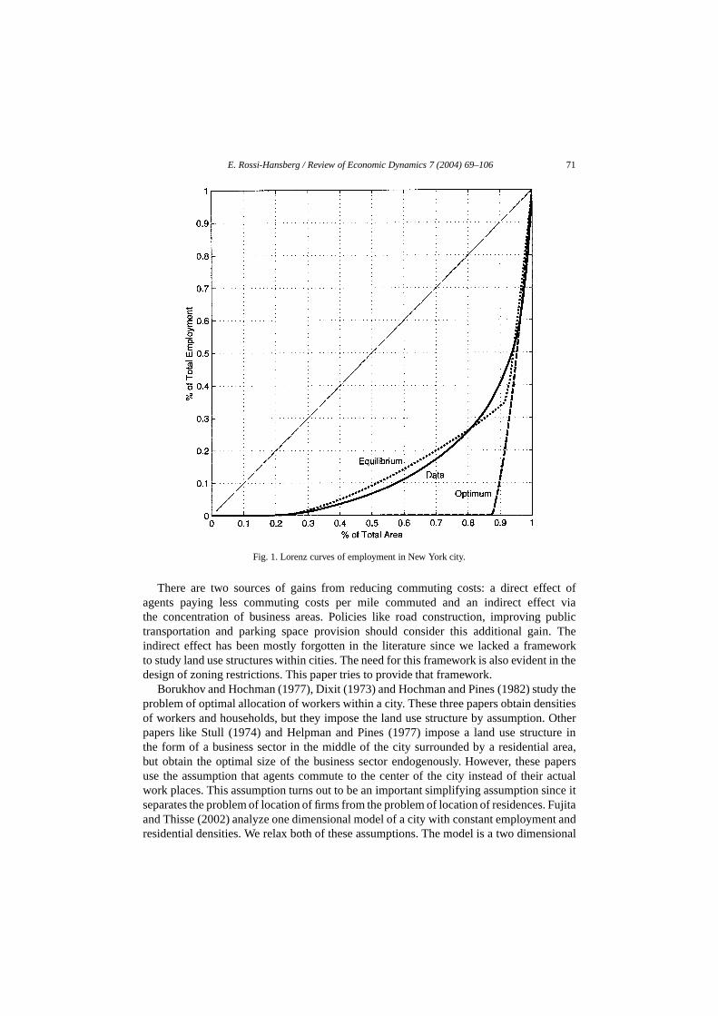
g. 1,Yorkell asrve formore
timalases.city.
eas. Intures.since
ces.ment ina for thevation in
characterize the optimal distribution of urban land, and use this analysis to design pthat improve the efficiency of equilibrium allocations.
Our focus is on allocations that maximize total production net of total consumptithe city. Or, equivalently, total rents. The theory determines the distribution of busineresidential land together with employment and residential densities at all locationscity. The two main forces that determine the optimal allocation of land in our theorspatial production externalities and commuting costs. The first force agglomeratesin clusters. The second disperses producers, so that workers can live close to theplaces. The trade-off between these two forces leads to optimal allocations thatdepending on the size of commuting costs and the form and degree of external eLow transport costs lead to a central business district with high employment density,higher transport costs result in low employment density or residential areas at theIf spillovers decline faster with distance, producers concentrate closer to the centercity, and business areas become smaller but with higher employment densities.
We use the model to analyze potential policies to improve efficiency in the city. Wethat location specific labor subsidies are sufficient to implement the optimal allocationequilibrium. In contrast, zoning restrictions cannot implement the optimal allocationthey can improve the efficiency of the equilibrium allocation, especially when commcosts are high.
Our results show that business land and employment are more concentratedoptimal than in the equilibrium allocation. In equilibrium, the higher commuting cthe more mixed areas in the city.1 In the optimum, mixed areas will disappear and the luse structure will resemble a Mills city (a central business center surrounded by resiareas, following Mills, 1967) for reasonably high commuting cost. Even higher commcost will yield multiple business or residential sectors. We will prove that it isnever optimalto have mixed areas in the city.
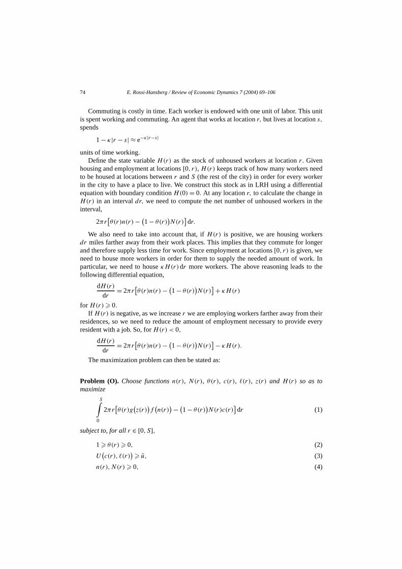
The higher concentration of the optimal employment density is illustrated in Fiwhere we have plotted the Lorenz Curve of employment concentration in NewCity.2 We find parameters so that the equilibrium Lorenz Curve fits the data as wpossible. We then use the same parameter configuration to compute the Lorenz Cuthe optimum. The figure suggests that employment in New York City should be muchconcentrated.
Another implication of the model is that the difference between the Pareto Opallocation and the equilibrium allocation is smaller as the cost of commuting decreIn equilibrium, when commuting costs are low, the allocation resembles a MillsThe same is true in the optimal allocation, but with more concentrated business arcontrast, high commuting costs imply different optimal and equilibrium land use strucOf course, the optimal employment density is greater than the equilibrium density,the effect on other firms of one firm employing more workers is internalized.
1 A mixed area is defined as a section of the city where workers live at, or very close to, their work pla2 The data comes from the 1992 Economic Census Zip Code Statistics. We calculate total employ
each Zip code by adding employment in the service, retail and manufacturing sectors. Employment datmanufacturing sector is only given as a range; we use the middle of the range as the employment obserthis sector.
E. Rossi-Hansberg / Review of Economic Dynamics 7 (2004) 69–106 71
ct ofct viapublic. Theworkin the
dy thesities. Otherture inl area,papersactual
ince itFujitant and
nsional
Fig. 1. Lorenz curves of employment in New York city.
There are two sources of gains from reducing commuting costs: a direct effeagents paying less commuting costs per mile commuted and an indirect effethe concentration of business areas. Policies like road construction, improvingtransportation and parking space provision should consider this additional gainindirect effect has been mostly forgotten in the literature since we lacked a frameto study land use structures within cities. The need for this framework is also evidentdesign of zoning restrictions. This paper tries to provide that framework.
Borukhov and Hochman (1977), Dixit (1973) and Hochman and Pines (1982) stuproblem of optimal allocation of workers within a city. These three papers obtain denof workers and households, but they impose the land use structure by assumptionpapers like Stull (1974) and Helpman and Pines (1977) impose a land use structhe form of a business sector in the middle of the city surrounded by a residentiabut obtain the optimal size of the business sector endogenously. However, theseuse the assumption that agents commute to the center of the city instead of theirwork places. This assumption turns out to be an important simplifying assumption sseparates the problem of location of firms from the problem of location of residences.and Thisse (2002) analyze one dimensional model of a city with constant employmeresidential densities. We relax both of these assumptions. The model is a two dime
72 E. Rossi-Hansberg / Review of Economic Dynamics 7 (2004) 69–106
ates inthese
Rossi-re ofthese
2) ands andlaxeste the
basicfersagelution
of thelution
tion 4ictions.nted intext.
labor.epends
and
mizeidere
tial
onomics
nough toumptiona onee will do
model since densities and externalities take into account that economic activity loca circular plane, a disc. However, we consider only symmetric allocations. None ofpapers designs policy instruments to improve efficiency.
Other papers like Fujita and Ogawa (1982), Berliant et al. (2002) and Lucas andHansberg (2002) (from now on LRH) determine only the equilibrium internal structuthe city and not the optimum. The difference is crucial, as pointed out above, since inmodels agglomeration is generated using production externalities.3 In particular, we willuse the same production externalities as in Lucas (2001). Fujita and Ogawa (198Berliant et al. (2002) assume a one dimensional city and constant densities of firmresidents. Although the latter article does introduce location specific capital. LRH reboth of these assumptions. We use the results in LRH extensively. They constituequilibrium allocation to which we compare the results of our model. Although theframeworks are identical, the way in which the equilibrium is calculated in LRH difsubstantially from the way in which the optimum is calculated in this paper. In LRH, wno arbitrage conditions are derived and they constitute an important part of the soalgorithm. For the optimum these conditions are not satisfied.
The paper is organized as follows. We present the model and study somenecessary conditions for an optimum in the next section. In Section 3 we provide a soalgorithm and prove the existence of a solution to the optimization problem. Secpresents some analytical results and the optimal labor subsidies and zoning restrSome numerical exercises that help us illustrate predictions of the theory are preseSection 5. Section 7 concludes. In Appendix A we prove the results presented in the
2. The model
We model a circular city where a single good is produced using land andPeople consume goods and residential land. There is a production externality that don where other firms locate. Workers allocate one unit of time between workingcommuting to their workplaces. Commuting is costly in time.
The objective is to maximize the value of land in the city. That is, we want to maxitotal production net of residents’ consumption (from now on ‘net output’). We will consonly symmetric allocations, where everything dependsonly on the distance from thcenter.4 Let n(r) be the number of workers per unit of business land at a distancer fromthe center (from now on ‘locationr ’), N(r) the number of residents per unit of residenland at locationr, θ(r) the proportion of land used for business purposes andc(r) and�(r)consumption and units of land per person.
3 See Anas et al. (1998) and Fujita et al. (1999) for other ways to generate agglomeration in urban ecmodels.
4 The assumption of symmetry is a strong assumption. Casual observation of metropolitan areas is erealize that people do not commute only to and away from the center to go to work. Nevertheless, the assis an important simplifying assumption of our theory. Without it, we can not reduce the external effect todimensional function and hence the stock of unhoused workers cannot be constructed sequentially as wbelow.
E. Rossi-Hansberg / Review of Economic Dynamics 7 (2004) 69–106 73
ment
otherhisse. It istionmand
Some1999),1993),ffects.ance,ce on2) findinsideat thee we
f an
ns andat both
quires am will
Firms produce using land and labor. At locationr, production per unit of land of a firmthat employsn(r) workers per unit of land is given by
g(z(r)
)f
(n(r)
),
wherez(r) denotes the productivity of a firm at locationr. Consider a circular city withradiusS. Productivity at each location is determined by an external effect of employthat declines exponentially with distance. As in Lucas (2001), we let
z(r)=S∫
0
ϕ(r, s)sθ(s)n(s)ds,
whereϕ(r, s) is given by
ϕ(r, s)= δ
2π∫0
e−δx(r,s,φ)dφ and x(r, s,φ)= [r2 − 2 cos(φ)rs + s2]1/2
.
That is, productivity at a particular location is a weighted average of employment atlocations. The particular form of the production externalities is arbitrary. Fujita and T(2002) derive this type of external effects from knowledge spillovers between firmspossible to show thatz(r) is also the reduced form of different types of agglomeraeffects. For example, if agglomeration effects are the results of differences in local deand increasing returns.
There are many empirical papers that test for spatial production externalities.examples are Ciccone and Peri (2002), Ciccone and Hall (1996), Dekle and Eaton (Ellison and Glaeser (1997), Glaeser et al. (1992), Henderson (2001), Jaffe et al. (Moretti (2002), and Rauch (1993). All these papers find evidence of agglomeration eIn particular, Dekle and Eaton (1999) find that the external effects decline with distparticularly in the financial services sector. Jaffe et al. (1993) also provide evidenpatents that suggests that interactions decline with distance. Glaeser et al. (199evidence that supports external effects among different industries and not onlyparticular industries. The same is true for Ciccone and Hall (1996) that show thdensity of economic activity determines productivity. This is important for us, sinchave a one good model and so the external effect affects all firms.5
Agents derive utility from residential land and consumption of goods. The utility oagent that consumesc(r) goods and occupies�(r) units of land is given by
U(c(r), �(r)
).
5 Another way of introducing agglomeration effects in urban economics models is via increasing returmonopolistic competition. Fujita and Thisse (2002) present a good summary of this literature. We believe thtypes of agglomeration effects result in identical optimal land use structures. However, this statement reproof which is left for future research. Using external effects or agglomeration effects internal to the firhave different policy implications.
74 E. Rossi-Hansberg / Review of Economic Dynamics 7 (2004) 69–106
unit
edrntialnn the
rsnger
rk. Inthe
eire every
Commuting is costly in time. Each worker is endowed with one unit of labor. Thisis spent working and commuting. An agent that works at locationr, but lives at locations,spends
1− κ |r − s| ≈ e−κ|r−s|
units of time working.Define the state variableH(r) as the stock of unhoused workers at locationr. Given
housing and employment at locations[0, r),H(r) keeps track of how many workers neto be housed at locations betweenr andS (the rest of the city) in order for every workein the city to have a place to live. We construct this stock as in LRH using a differeequation with boundary conditionH(0)= 0. At any locationr, to calculate the change iH(r) in an intervaldr, we need to compute the net number of unhoused workers iinterval,
2πr[θ(r)n(r)− (
1− θ(r))N(r)
]dr.
We also need to take into account that, ifH(r) is positive, we are housing workedr miles farther away from their work places. This implies that they commute for loand therefore supply less time for work. Since employment at locations[0, r) is given, weneed to house more workers in order for them to supply the needed amount of woparticular, we need to houseκH(r)dr more workers. The above reasoning leads tofollowing differential equation,
dH(r)
dr= 2πr
[θ(r)n(r)− (
1− θ(r))N(r)
] + κH(r)
for H(r)� 0.If H(r) is negative, as we increaser we are employing workers farther away from th
residences, so we need to reduce the amount of employment necessary to providresident with a job. So, forH(r) < 0,
dH(r)
dr= 2πr
[θ(r)n(r)− (
1− θ(r))N(r)
] − κH(r).
The maximization problem can then be stated as:
Problem (O). Choose functions n(r), N(r), θ(r), c(r), �(r), z(r) and H(r) so as tomaximize
S∫0
2πr[θ(r)g
(z(r)
)f
(n(r)
) − (1− θ(r)
)N(r)c(r)
]dr (1)
subject to, for all r ∈ [0, S],1 � θ(r)� 0, (2)
U(c(r), �(r)
)� u, (3)
n(r),N(r)� 0, (4)
E. Rossi-Hansberg / Review of Economic Dynamics 7 (2004) 69–106 75
s to betilityntry.
traintrminess at the
last
eThe
to
�(r)= 1
N(r), (5)
H(0)= 0 and H(S)� 0, (6)
z(r)=S∫
0
ϕ(r, s)sθ(s)n(s)ds. (7)
Constraint (2) states that the proportion of land used for business purposes habetween 0 and 1. (3) guarantees that every household gets at least a reservation uu.
One useful way of thinking about this constraint is to let the city be part of a big couThen u is the utility that an agent could get if he migrates to some other city. Cons(4) guarantees that the density of workers and residents is positive and (5) detethe amount of land per person. (6) guarantees that the stock of unhoused workerboundary of the city is zero. That is, that all workers are housed in the city. Theconstraint determines the external effect as discussed above.
The Hamiltonian for the problem, without considering (3) and (7), is given by
G(r,H,n,N, θ, c, z, λ)= 2πr[θ(r)g
(z(r)
)f
(n(r)
) − (1− θ(r)
)N(r)c(r)
]− λ(r)
[2πr
[θ(r)n(r)− (
1− θ(r))N(r)
] + κ∣∣H(r)∣∣].
Including constraints (3) and (7) we can built a Lagrangian given by
L(r,H,n,N, θ, c, z, λ, ξ,µ)=G(r,H(r), n(r),N(r), θ(r), c(r), z(r), λ(r)
)+ ξ(r)
[U
(c(r),
1
N(r)
)− u
]
+S∫
0
µ(s)
[ S∫0
ϕ(s, r)rθ(r)n(r)dr − z(s)
]ds,
whereξ(r) is the Lagrange multipliers associated with (3),λ(r) is the co-state variablassociated with (6) andµ(r) is the Lagrange multiplier associated with constraint (7).co-state variableλ(r) represents the cost of employing an extra worker at locationr. It isthe costs of giving the worker land at some location in(r, S] and enough consumptionobtain utility u.
The first-order conditions after eliminating the Lagrange multipliersξ(r) andµ(r) are,for all r ∈ [0, S],
g(z(r)
)f ′(n(r)) � λ(r)−
S∫0
sθ(s)g′(z(s))f (n(s)
)ϕ(s, r)ds, (8)
c(r)+ U� � λ(r), (9)
N(r)Uc
76 E. Rossi-Hansberg / Review of Economic Dynamics 7 (2004) 69–106
orker
ehind
cing atgut
n
eress or
state
st
te
λ(r)[n(r)+N(r)
]�
[g(z(r)
)f
(n(r)
) +N(r)c(r)]
+ n(r)
2π
S∫0
sθ(s)g′(z(s))f (n(s)
)ϕ(s, r)ds, (10)
where the first two conditions hold with equality ifn(r) > 0 andN(r) > 0. In the lastcondition, the left-hand side is greater ifθ(r) > 0, smaller ifθ(r) < 0, and equal to theright-hand side ifθ(r) ∈ (0,1).
These equations plus the constraints
U
(c(r),
1
N(r)
)= u,
S∫0
ϕ(r, s)sθ(s)n(s)ds = z(r),
and (6), form the system of first-order conditions.The last terms (8) represents the effect on other locations of hiring an extra w
at locationr. Since this term is positive, iff is concave,n(r) will be larger than ifthe externality was not internalized. It is also useful to understand the intuition bcondition (10). Rewrite it as
g(z(r)
)f
(n(r)
) + χ(r)− λ(r)n(r)�N(r)[λ(r)− c(t)
],
where
χ(r)= n(r)
2π
S∫0
2πsθ(s)g′(z(s))f (n(s)
)ϕ(s, r)ds.
Then, the first term on the left hand side is total output per unit of land if locationr is abusiness sector. The second is the total gain in output at other locations from produlocationr, caused by the external effect, and the third represents the cost of employinn(r)
workers. On the right hand side,N(r)[λ(r)− c(t)] are the benefits in terms of net outpof housingN(r) worker at locationr. As we mentioned before,λ(r) has the interpretatioof the unit cost, land plus consumption, of employing an extra worker. So[λ(r)− c(t)] isthe gain per resident of assigning the land at locationr for housing. Hence, the first-ordcondition compares the benefits, in terms of net output, of land being used for businresidential purposes.
The Maximum Principle provides an extra condition on the behavior of the co-variable. Namely,
∂λ(r)
∂r= −∂G(r)
∂r=
{−κλ(r) if H(r) > 0
κλ(r) if H(r) < 0for all r ∈ [0, S], (11)
and Pontryagin Maximum Principle also requiresλ to be continuous. The system of firorder conditions can be solved forn, N , c, z given λ(0) andθ . Using (6) we can thensolve for the value ofλ(0). Given this, we can use the condition above to calculaλat all locationsr whereH(r) > 0 or H(r) < 0. If H(r) = 0, then∂λ(r)/∂r = −κλ(r)
E. Rossi-Hansberg / Review of Economic Dynamics 7 (2004) 69–106 77
.
d the
ect tong., onectionandt way.area, the
old, if
if θ(s) = 1 for s > r arbitrarily close tor and∂λ(r)/∂r = κλ(r) if θ(s) = 0 for s > r
arbitrarily close tor. If θ(s) ∈ (0,1) for s > r arbitrarily close tor, then if
θ(r)n(r)− (1− θ(r)
)N(r) > 0, we know that
∂λ(r)
∂r= −κλ(r),
since we are accumulating unhoused workers soH(s) > 0 andλ is a continuous functionIf
θ(r)n(r)− (1− θ(r)
)N(s) < 0, then
∂λ(r)
∂r= κλ(r),
since we are decreasing the amount of unhoused workers. Finally, if
θ(r)n(r)− (1− θ(r)
)N(r)= 0,
we can use this equation to solve for∂λ(r)/∂r.The above description implies that we can solve for all variables in terms ofθ. The next
section provides an algorithm to find the optimal land use structure, summarized byθ.
3. Optimal land use structure
All the exposition until now shows how to obtain the different controls, the state, anco-state given a function of land use proportions,θ. But it does not provide an algorithmto find the optimal land use structure. Notice that the first-order condition with respθ(r) can be used only whenθ(r) ∈ (0,1) since in both other cases constraint (2) is bindiOptimization theory does not provide a good way of dealing with corner solutionspossible way of dealing with this problem is to compute the value of the objective funfor all possible combinations (given a minimum lot size). This solution is very costlywould not add to the understanding of the problem at hand. We proceed in a differenThe first-order condition in (9) implies that if, for example, locationr is assumed to bepure business area, and it is actually optimal for this area to be a pure business aconstraintθ(r)� 1 must be binding. Hence
[g(z(r))f (n(r))+N(r)c(r)] + χ(r)
[n(r)+N(r)] > λ(r).
Definet (r) by
t (r)≡ [g(z(r))f (n(r))+N(r)c(r)] + χ(r)
[n(r)+N(r)] .
Using the same type of reasoning for all possible assumptions onθ(r), we know that at theoptimum,
θ(r)= 1 iff t (r) > λ(r),
θ(r) ∈ (0,1) iff t (r)= λ(r), and
θ(r)= 0 iff t (r) < λ(r).
Every time we propose a solution we need to check if the above inequalities hthey do not, the allocation is not a solution to Problem (O).
78 E. Rossi-Hansberg / Review of Economic Dynamics 7 (2004) 69–106
y thatmum ism tor the
ables,
tion
zero.
nn 3).ence ofhelts we
, and
In order to find a maximum, a solution to Problem (O), it seems that a strategassumes some land use structure and then tests if the solution is actually a maxinot going to take us too far. In this section we will provide a general solution algorithfind the solution of this problem. The basic idea is to start with some initial guess fofunctionθ, compute the corresponding densities, productivity function, and state variand then use the previous equations to obtain a new functionθ.
Define an operatorT :M → M (whereM denotes the space of measurable funcf (r) : [0, S] → [0,1]) that maps land use proportion functionsθ into land use proportionfunctions. In particular we let
(T θ)(r)=
1 if t (r) > λ(r),N(r)
N(r)+n(r) if t (r)= λ(r),
0 if t (r) < λ(r).
Notice that in the case wheret (r)= λ(r), we let (T θ)(r)= N(r)N(r)+n(r) . This has to be
the case for
θ(r)n(r)− (1− θ(r)
)N(r)= 0
to hold. If this equation is not satisfies we know thatλ(r) will be decreasing at rateκ orgrowing at rateκ , and so the equality can only hold for a set of Lebesgue measureIf the constraint is satisfied, then we may haveH(r)= 0 for an interval of locations withpositive Lebesgue measure, a mixed sector.
A solution that satisfies the first-order condition forθ, will have to satisfy
T θ = θ.
If we can find a functionθ that is a fixed point of the operatorT , then we have found aallocation that satisfies all the necessary conditions for a maximum (See Propositio
The existence of a solution that satisfies the necessary conditions, and the exista fixed point of operatorT , is proven in the following propositions and theorem. All tproofs of theorems and propositions are presented in Appendix A. To prove the resuimpose the following assumptions.
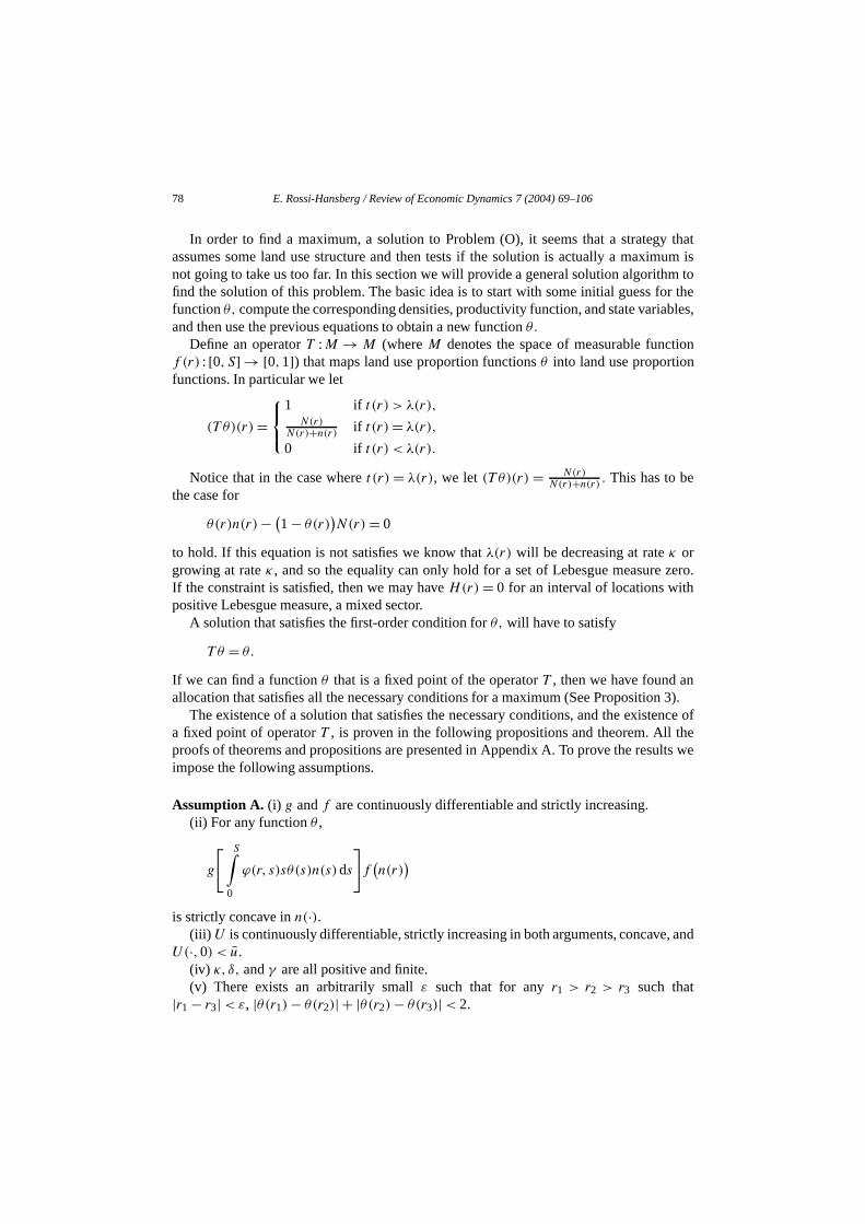
Assumption A. (i) g andf are continuously differentiable and strictly increasing.(ii) For any functionθ ,
g
[ S∫0
ϕ(r, s)sθ(s)n(s)ds
]f
(n(r)
)
is strictly concave inn(·).(iii) U is continuously differentiable, strictly increasing in both arguments, concave
U(·,0) < u.(iv) κ, δ, andγ are all positive and finite.(v) There exists an arbitrarily smallε such that for anyr1 > r2 > r3 such that
|r1 − r3|< ε, |θ(r1)− θ(r2)| + |θ(r2)− θ(r3)|< 2.
E. Rossi-Hansberg / Review of Economic Dynamics 7 (2004) 69–106 79
jectiveove
l areas.
traf
y cross
. Inmixed
inessthe
.
ease, in
xednther
Two of these assumptions require an explanation. Part (ii) guarantees that the obfunction is concave inn(·). Part (iii) guarantees that lot sizes are uniformly bounded abzero as we increaseκ arbitrarily.
Proposition 1. Under Assumption A, given θ there exists a unique set of functions {n∗, N∗,c∗, �∗, z∗, H ∗, λ∗} that satisfies the first-order conditions and the Maximum Principleconditions.
Proposition 2. Under Assumption A, there exists a function θ∗ such that
T θ∗ = θ∗.
Proposition 3. Under Assumption A, there exists a set of functions {θ∗, n∗, N∗, c∗, �∗,z∗, H ∗, λ∗} that satisfies the first-order conditions, the Maximum Principle conditions andT θ∗ = θ∗.
We now prove that the solution consists only of pure business and pure residentia
Theorem 1. Under Assumption A, the optimal land use structure has no mixed areas. Thatis θ∗(r) ∈ {0,1}, except for sets with zero Lebesgue measure in [0, S].
Mixed area require two conditions,H(r) = 0 and that the value of adding an exworker equals the value of housing an extra resident,t = λ. The idea behind the proof oTheorem 1 is that this can happen, but only at some specificr and not for an interval withpositive Lebesgue measure. This is called a transversal crossing, the two values mabut their slope with respect tor is different.
Mixed areas can be part of the equilibrium city structure, as shown in LRHequilibrium, wages at the center can adjust so that the two necessary conditions for aarea are satisfied. The difference is that in the efficient allocation changes inλ(0) will alsochangeχ(r) (the effect of employing an extra worker at locationr in the production ofother firms in the city), which in turn changes the gains from using the location for buspurposes. Thus, in general there is noλ(0) that satisfies the conditions necessary forexistence of a mixed area.
The next proposition uses Theorem 1 to prove existence of an efficient allocation
Proposition 4. Under Assumption A, there exists a set of functions {θ∗, n∗, N∗, c∗, �∗,z∗, H ∗, λ∗} that solves Problem (O).
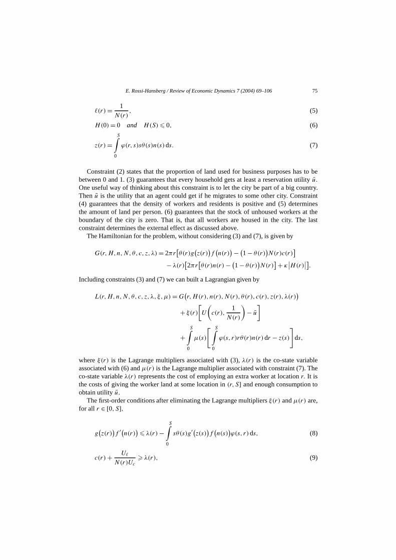
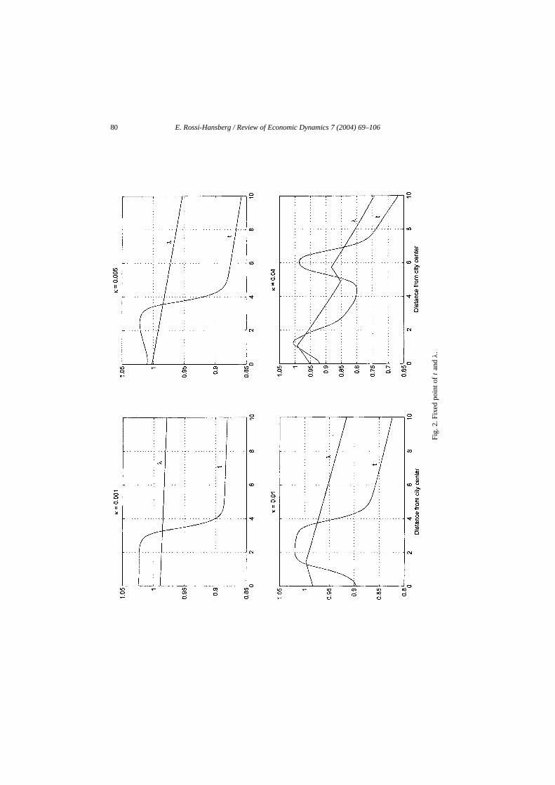
Figure 2 illustrates the fixed point of the iterations oft andλ, that in turn determine thfixed point ofθ. We use the parameter values presented in Section 5 as the base cparticularκ = 0.005. The initial land use proportions function isθ0(r) = 1 for r ∈ [0,2]andθ0(r) = 0 for r ∈ (2,10]. The fixed point of the operator is given byθ∗(r) = 1 forr ∈ [0,3.5] andθ∗(r) = 0 for r ∈ (3.5,10]. We have guaranteed the existence of a fipoint, but not the convergence of the iterates ofθ to that fixed point. Hence, the fixed poicould depend on the initial functionθ0. We computed the same experiment with ot
80 E. Rossi-Hansberg / Review of Economic Dynamics 7 (2004) 69–106
Fig
.2.F
ixed
poin
toft
andλ
.

E. Rossi-Hansberg / Review of Economic Dynamics 7 (2004) 69–106 81
jectiveectors,actual
f landr). Thes, but itn twom (O)uset, itum of
odel:f
he city.ork
nineas and
case.ecrease
nessesalities
ies tois to
e twoolicies.
s fromManyended998).
rnalityfirmsr apart
if
initial functions and obtained the same result. We also computed the value of the obfunction for different locations of the borders between the business and residential sand in all case obtained smaller values. All of this leads us to believe that this is thesolution to Problem (O) and not a local maximum or saddle point.
The method proposed is more efficient than looking at all possible combinations ouse structures. Even if we only look at a restricted set (e.g. only one business sectoreason is that each iteration of the operator is equivalent to testing a set of boundarieallows us to move in the right direction and without testing all boundaries in betweeiterations. It also guarantees that the solution found is an extreme point of Probleover all possible combinations of land use structures. Finally, if different initial landproportion functionsθ0 are used, and all of them converge to the same fixed poingives some assurance that the fixed point is unique and therefore a global maximthe problem.
Figure 2 also presents exercises for three otherκ values: 0.001, 0.01, and 0.04. Theκ values where chosen to illustrate different possible allocations of land in the ma central business district, with high (κ = 0.001) and low (κ = 0.005) densities, a ring obusinesses (κ = 0.01) and two rings of businesses (κ = 0.04). If κ = 0.001, the centerof the city is used for business purposes and densities are high at the center of tFor κ = 0.01 agents will commute to and away from the center in order to get to wsince there is a residential core. Hence,λ first increases at rateκ, has a kink, and thestarts decreasing at rateκ. Finally, whenκ = 0.04, the center is residential and we obtatwo rings of business areas, together with rings of residences between business arat the boundary. All examples use the same initial land use function as the baseHow does the land use structure change as we increase commuting costs and dexternalities? The results suggest that the solution will have several rings of busiwith rings of residences in between them. Larger commuting costs and lower externwill be associated withmore rings of businesses.
4. Optimal subsidies and zoning policies
The analysis of optimal urban structure can be used to design optimal policimprove the efficiency of equilibrium allocations in the same setup. The first stepdefine the marginal product of labor and the value of land in the optimum. With thesconcepts in hand, we then proceed to design and characterize the effect of different pThe main problem is to find policies that implement the optimum as an equilibrium.
One argument against designing policies using our framework, is that is abstractcongestion costs. Commuting costs are the only force balancing agglomeration.papers in the urban economics literature focus on congestion and the policies recommto reduce its costs (see for example Dixit, 1973; Anas and Xu, 1999; or Wheaton, 1We do not model congestion directly, although it can be modeled as part of the exteparameters. δ can be thought of as consisting of two parts, a positive part that makeswant to be close to each other, and a negative part that makes firms want to be fa(the congestion effect). In this paper we focus on positiveδ, so the positive spillover ismore important than the negative one resulting from congestion. In this framework,δ is
82 E. Rossi-Hansberg / Review of Economic Dynamics 7 (2004) 69–106
s dodin the
include
ansamewages
o othercan be
tion oflower
abor.riumof
not positive, firms do not agglomerate in cities. So the fact that in reality there citieexists implies thatδ > 0. Some evidence on the need of high positiveδ values is presentein Lucas (2001). This reasoning leads us to believe that the omission of congestionmodel does not invalidate the results in the paper. Nevertheless, further attempts tocongestion in this framework could provide interesting insights.
4.1. Marginal product of labor and the value of land
Given n∗, N∗, z∗, θ∗ andλ∗ we can calculate the land rents and wages that, inequilibrium context, would make agents and firms at a particular location choose theamount of workers, land, and consumption, as the planner. These are not equilibriumand land rents since for these prices agents and firms have incentives to move tlocations. In business areas, the value of land and the marginal product of laborcomputed using
q(r)= g(z∗(r)
)f
(n∗(r)
) −w(r)n∗(r)
and the implied first-order condition of the firm’s problem
w(r)= g(z∗(r)
)f ′(n∗(r)
).
Solving the system, the value of land and the marginal product of labor can forθ(r)= 1be given by
q(r)= g(z∗(r)
)f
(n∗(r)
) − g(z∗(r)
)f ′(n∗(r)
)n∗(r),
w(r)= g(z∗(r)
)f ′(n∗(r)
) = λ∗(r)−S∫
0
sθ∗(s)g′(z∗(s))f (n∗(s)
)ϕ(s, r)dr,
where the second equality in the second equation comes from the first-order condiProblem (O). Notice that the marginal product of labor in pure business sectors isthan the equilibrium wage where wages are given by
w(r)= λ∗(r).
The fact that firms internalize the externality results in a lower marginal product of lTo take full advantage of spillovers, optimal employment is greater than in equilibwhich implies a lower marginal product, given decreasing returns to labor. The slopeλ∗has to be the same here than in equilibrium, although not the level.
The consumer problem is given by
w(r)= max
[c∗(r)+ q(r)
(1
N∗(r)
)],
s.t. u�U
(c∗(r),
1
N∗(r)
)and the corresponding first-order condition is
q(r)= U�.
Uc

E. Rossi-Hansberg / Review of Economic Dynamics 7 (2004) 69–106 83
n.
izeitrageyone isncethat
or anditions
sureditions
e
nd is
Solving the system, the value of land and the marginal product of labor forθ(r)= 0 are
q(r)= U�(c∗(r), 1
N∗(r))
Uc(c∗(r), 1
N∗(r)) =N∗(r)λ∗(r)−N∗(r)c∗(r),
w(r)= c∗(r)+ U�(c∗(r), 1
N∗(r))
Uc(c∗(r), 1
N∗(r))(
1
N∗(r)
)= λ∗(r),
where the second inequality in the first equation follows from the first-order conditio
4.2. Optimal subsidies
The definition of equilibrium in LRH determines that in equilibrium firms maximprofits, residents minimize expenditures given a reservation utility, wage no arbconditions are satisfied, land is assigned to its highest value (highest bid rent), everhoused, and the externality function,z, is constructed as described in constraint (7). Heif we want to implement the optimal allocation as an equilibrium, we need to checkthe wage no arbitrage conditions are satisfied by the optimal marginal product of labthat land is assigned to its highest value at the optimal value of land. All other condare constraints in Problem (O).
In order to implement the optimal allocation as an equilibrium, we need to makethat the policy that we design satisfies the wage no arbitrage conditions. these conare given by
w(r)=K1e−κr if H(r) > 0 and w(r)=K2eκr if H(r) < 0,
for some constantsKi , i = 1,2.In our case,λ∗ does satisfy these conditions since, as we discussed before,
∂λ∗(r)∂r
={−κλ∗(r) if H(r) > 0,
κλ∗(r) if H(r) < 0.
Nevertheless, the optimal marginal product of labor functionw(r) does not. We havshown that in business areas,
w(r)= λ∗(r)−S∫
0
sθ∗(s)g′(z∗(s))f (n∗(s)
)ϕ(s, r)dr.
So a policy that satisfies the wage no arbitrage conditions is a labor subsidyτ to firmsof the form
τ (r)=
S∫0
sθ∗(s)g′(z∗(s))f (n∗(s)
)ϕ(s, r)dr if θ∗(r) > 0,
0 if θ∗(r)= 0.
The second condition that we need to check, for any proposed policy, is that laassigned to its highest value. That is, we need
84 E. Rossi-Hansberg / Review of Economic Dynamics 7 (2004) 69–106
e that
ments
rginalnd isLRHtimalies is
y firmserage
q(r)|θ(r)=1> q(r)|θ(r)=0 for a business sector,
q(r)|θ(r)=1 = q(r)|θ(r)=0 for a mixed sector, and
q(r)|θ(r)=1< q(r)|θ(r)=0 for a residential sector.
One can show that this is always the case in the optimal allocation. For this, suppos
[g(z∗(r))f (n∗(r))+N∗(r)c∗(r)] + χ(r)
[n∗(r)+N∗(r)] > λ∗(r),
or
g(z∗(r)
)f
(n∗(r)
) − λ∗(r)n∗(r)+ χ(r) > N∗(r)λ∗(r)−N∗(r)c∗(r).
From the definition ofq(r)|θ(r)=1, we know that
q(r)|θ(r)=1 = g(z∗(r)
)f
(n∗(r)
) −w(r)|θ(r)=1n∗(r)
= g(z∗(r)
)f
(n∗(r)
) − λ∗(r)n∗(r)+ χ(r).
Notice also that
w(r)|θ(r)=0 = c∗(r)+ q(r)|θ(r)=0
(1
N∗(r)
),
which implies that
q(r)|θ(r)=0 =N∗(r)w(r)|θ(r)=0 −N∗(r)c∗(r)=N∗(r)λ∗(r)−N∗(r)c∗(r).
Hence in a business sector of the optimal allocationq(r)|θ(r)=1 > q(r)|θ(r)=0 is alwayssatisfied. The proof is analogous for the cases of mixed and residential sectors.
We are ready to formally state the result that the subsidy proposed above implethe optimal allocation as an equilibrium.
Theorem 2. A labor subsidy τ of the form
τ (r)=
S∫0
sθ∗(s)g′(z∗(s))f (n∗(s)
)ϕ(s, r)dr if θ∗(r) > 0,
0 if θ∗(r)= 0,
implements the optimal allocation as an equilibrium.
Proof. We have shown above that with this subsidy the optimal land values and maproducts of labor satisfy the wage no arbitrage condition and the condition that laassigned to its highest value. Since all other parts of the definition of equilibrium inare either imposed as constraints of Problem (O), or implied by the definition of opland value and marginal product of labor, the equilibrium allocation with labor subsidan optimum. ✷
The subsidy proposed in Theorem 2 is a subsidy that the government should paso that they face lower labor costs, and hence hire more workers (in equilibrium av
E. Rossi-Hansberg / Review of Economic Dynamics 7 (2004) 69–106 85
y askvy a
mentctually
es nottion.blem.ducingthese
rtation
e city.s area,
licy to
blemlaboreme anthe
all theefits
ncefirms
in thetweenissue
willzoningthe
by forple, berictions
wages will increase, and since reservation utility is fixed, residential rents). One mahow, in this model, a government would pay for the subsidy. One possibility is to leflat tax on land owners. The implied tax is given by
τ+ = 1
2πS
S∫0
τ (s)ds
per unit of land. This tax will not distort rents and would balance the city governbudget. Notice that in this model we have absentee landlords so we are not amodeling the decision of buying land in the city or in different cities.
In reality we do not observe these types of subsidies, and although this doundermine their optimality, it is puzzling that we do not see any efforts in this direcA closer look at City Government policies may give us a possible answer to the proFor example, parking lots construction by government agencies may be a way of rethe costs of working at business centers, thereby actually subsidizing workers inareas. Highway improvement and construction and investments in public transpoare other interesting examples.
4.3. Zoning policy
Suppose the city government can determine land use in different sections of thThat is, the city government can determine if some section of the city is a businesa residential area or a mixed area (the government has the power to determineθ(r)). In thiscase, we can ask what the best set of restrictions is, and if zoning is an effective poincrease net output in a city.
The optimal land use does not solve the optimal zoning policy problem. This prois given by Problem (O) plus the constraints that the optimal marginal product ofdeclines or increases at rateκ throughout the city. That is, the optimal zoning problimplies solving for the optimal land use structure restricting the allocation to bequilibrium givenθ . We do not solve that problem in this paper, but we do analyzecase where we impose the optimal land use as a restriction. This is what we cequilibrium with zoning restrictions. The exercise yields a lower bound for the benof zoning restrictions since the optimal land use structure is a feasibleθ .
The equilibrium with zoning restrictions will not internalize the externality, and hewill not be optimal, but it will take advantage of higher external effects caused bybeing closer to each other (in Theorem 1, we proved that there are no mixed areasoptimal land use structure). Hence, net output will increase. How much of the way bethe optimum and the equilibrium will this type of restrictions take us is a numericaland will be studied in the next section.
One important feature of the equilibrium with zoning restrictions is that land rentsnot be continuous at the boundary between business and residential sectors. Therestriction will be binding, since the equilibrium land use structure is different thanoptimal land use structure. So there are incentives for some land owners to lobchanges in the zoning restrictions. Given the restrictions, some firms may, for examready to pay higher rents in residential sectors than residents. Of course, if the rest
86 E. Rossi-Hansberg / Review of Economic Dynamics 7 (2004) 69–106
fect isplesn be
riumthe
l citylandtive ofristicsngese usedtant in
utility
incomeof
yments
rgestuld alsoaverage
are lifted altogether, we return to the equilibrium outcome, and since the external eflower in equilibrium, land rents will go down. In the next section we will presents examof the equilibrium with zoning restrictions where the discontinuities in land rents caobserved.
5. Numerical exercises
In this section we use numerical exercises to illustrate some of the equilibpossibilities of the model. We will set the different parameters values followingprevious literature and then vary key parameters to illustrate their effect on optimastructure, in particularκ andδ. These two parameters are crucial in determining theuse structure within a city and the results are very sensitive to their values. The objecthese exercises is not to obtain numerical implications that match particular characteof a specific city, but to illustrate how optimal allocations and policies react to chain key fundamental parameters. The model is admittedly very stylized and should bas a conceptual framework to understand the interaction of forces that are impordetermining urban structure, not to obtain quantitative implications.
In all the numerical exercises we use a Cobb–Douglas specification for thefunction,
U(c, �)= cβ�1−β,
and the production function,
f (n)=Anα.
We also let
g(z)= zγ .
In the numerical exercises shown below we use the following parameter values:
α β γ A u κ δ S
0.95 0.9 0.04 1 1 0.005 5 10
Caselli and Coleman (2001) show that the share of land rentals in nonfarm businessin the US is around 5%, hence we letα = 0.95. Roback (1982) estimates the shareincome going to mortgage payments to be 0.178, since this includes structures (pafor the actual house not only land) we reduce the number to 0.1 and letβ = 0.9. Lucas(2001) uses Japanese Land Rent data to argue that a reasonable value ofγ is 0.04. A andu are set arbitrarily at 1.6 The city size is also set arbitrarily atS = 10 miles.7 These
6 Another possibility is to calibrateu such that the population size is about 100,000. In a sample of the la1083 cities in the USA, the average population size was 105412 according to the 1990 Census. We cocalibrateA such that the average per capita monetary income is about 15000 US dollars. In 1990, themonetary income per capita in a sample of 1083 cities was 14867 US dollars.
7 The average land area in 1990 of a sample of 1083 cities was 38.78 sqm.
E. Rossi-Hansberg / Review of Economic Dynamics 7 (2004) 69–106 87
s with
d fromtheymiles
orm
metersin the
rithmmn the
dlations
aluesentialreas arearginal
ation.latively
therms areductionkers atearby.The
istance.
e
parameter values are fixed throughout the paper. We will perform comparative staticall the remaining parameters. Forδ = 5 see Lucas (2001) and LRH, forκ = 0.005, noticethat in a sample of 1083 cities, people commute 20.57 minutes on average to anwork. If they work around 8 hours a day (including commuting), this implies thatspent 4.29 percent of their time commuting. So if they commute on average about 10it implies aκ = 0.00429. Since some of these calculations are very loose, we will perfnumerical exercises for a wide range of values ofκ .
In order for Assumption A to hold for this particular specification, we needα,β, γ > 0,β,α < 1, and 1−α > γ . Clearly these restrictions are satisfied for the base case paravalues presented above. For an interpretation of 1− α > γ in the urban economicliterature, see Lucas (2001) or Fujita et al. (1999). We formalize this statementfollowing lemma, proven in Appendix A.
Lemma 1. If U,f and g are Cobb–Douglas as specified above, α,β, γ > 0, β,α < 1 and
1− α > γ,
then Assumption A is satisfied.
We solve the nonlinear system of equations in Section 2 using MATLAB. The algosolves the system given a functionθ. We let 1r = 0.01 and so we have a systeof S5/1r + 1 equations in the same number of unknowns. As a result we obtaioptimal densitiesn∗,N∗, the optimal consumption per person,c∗, the optimal productivityfunctionz, and the co-stateλ, at all locations and as a function ofθ. To find the optimalθ we iterate using the operatorT until the sequence ofθ functions converges. As notebefore this sequence does not have to converge, although it does in all the simupresented.
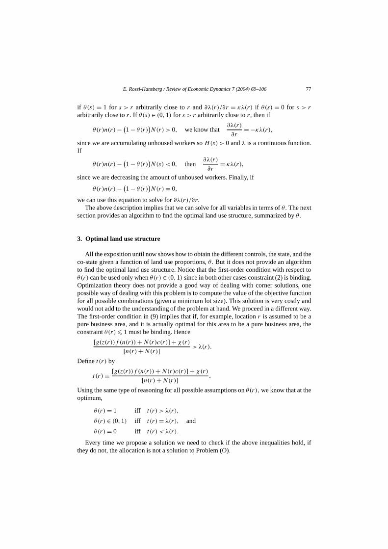
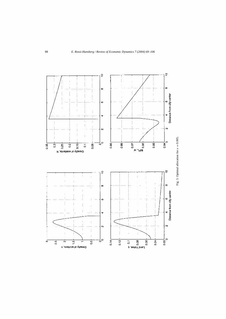
For the base case parameters, we obtain a business area with a radius of 3.5 miles. Therest of the city is residential. In LRH, the equilibrium city for the same parameter vhas a mixed sector in the middle with a radius of about 4 miles, followed by a residarea of about two miles, and a residential sector at the boundary. Hence, business amore concentrated at the optimum. The densities of workers and households, and mproduct of labor and land values are presented in Fig. 3.
Figure 3 shows the main forces that are at work to determine the optimal allocThe density of workers is relatively high at the center, since business sectors are reclose in all directions which increases the external effect. As we move away fromcenter the external effect decreases. Even though the external effect decreases, ficloser to the residential areas. Being closer to residential areas implies that less prohas to be spent in commuting costs. The result is an increase in the amount of worthese locations. The higher employment density increases the productivity of firms nThe productivity function and the optimal values of land follow this same pattern.density of households declines since it is a function ofλ. As we move away from thecenter, the cost of housing workers increases since commuting costs increase with dConsumption decreases too, since these households are living in larger land lots (�= 1/Ngrows) and their utility is constant atu. The marginal product of labor follows first th
88 E. Rossi-Hansberg / Review of Economic Dynamics 7 (2004) 69–106
Fig
.3.O
ptim
alal
loca
tion
forκ
=0.
005
.

E. Rossi-Hansberg / Review of Economic Dynamics 7 (2004) 69–106 89
idents.h
are
ted in
notrest ofmuting
s from
n
ther
g. 2rerative
ictionressn thecitiessmall
d thisutputted theic land
ln theis, then, but
d by a
ts andlarger
same pattern as the density of workers and then the pattern of the density of resSinceH(r) is positive for allr, λ decreases at rateκ throughout the entire city. At eaclocation in business sectors the optimal marginal product of labor is lower thanλ, sincefirms hire more workers than the profit maximizing amount. At the optimum weinternalizing the external effect. In an equilibrium allocationw(r) = λ(r). The trade-offbetween higher external effects and proximity to residential sectors is also illustraFig. 4 for commuting costsκ = 0.001.
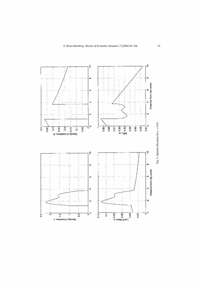
If we increaseκ to 0.01, the high commuting cost imply that the monocentric city isoptimal. In this case the business sector is a ring around the center of the city. Thethe city, that is the center and the areas near the boundary are residential. Since comcosts are higher, proximity to residents becomes more important than the spillovernearby firms. Agents leaving near the center will commuteaway from the center to go towork. Agents living close to the boundary will commuteto the center to go to work, as iall other cases. These results are presented in Fig. 5.
In Fig. 2 we presented the fixed point oft andλ. Whenκ = 0.005, the fixed point oft andλ is such thatt (r) � λ(r) at the center (the business district). For locations faraway from the centert (r) < λ(r) and soθ(r)= 0 (the residential area). That is,
θ∗(r)={
1 if r ∈ [0,3.5],0 if r ∈ [3.5,0],
is a fixed point of the operatorT for κ = 0.005. Forκ = 0.001 andκ = 0.01 the figureshows how the fixed point oft andλ imply the land use structure described above. In Fiwe also presented a numerical example forκ = 0.004. The result is a land use structuwith two rings of businesses. In what follows we drop this case and focus on compastatics where we increaseκ to 0.01 and decreaseκ to 0.001 relative to the base case.
Given our focus on symmetric allocations, we can ask how important is the restrthat the whole land area,πS2, has to be used to construct only one city. We can addthis question numerically. We start with the optimum presented in Fig. 5, break dowtotal land area of the city in two, and compute the optimum for each of the smallerassuming no external effects between them. The results imply that the sum of the twocities net output is smaller than the net output of the initial city by 13%. We repeateexercise by breaking down the original city in four and eight cities. The sum of net ois decreasing in the number of cities. The smaller the land area, the more concentrabusiness sectors. In particular, for the cases of 4 and 8 cities we obtain monocentruse structures.8
In Fig. 6 we present the optimal density of workers (timesθ ) resulting from the optimaland use structure (same as in Fig. 2) and the optimal density of workers giveequilibrium land use structure. In both curves the external effect is internalized. Thatdashed line is not the equilibrium density of workers for this parameter configuratiothe optimal density of workers restricting land use to be as in equilibrium. Forκ = 0.005,equilibrium land use is given by a mixed area of 4.2 miles at the center, surrounde
8 It is clear that the result will not hold if we start doubling the size of the city. The extra commuting costhe implied less concentrated business areas will eventually offset the gains in productivity implied by thecity.
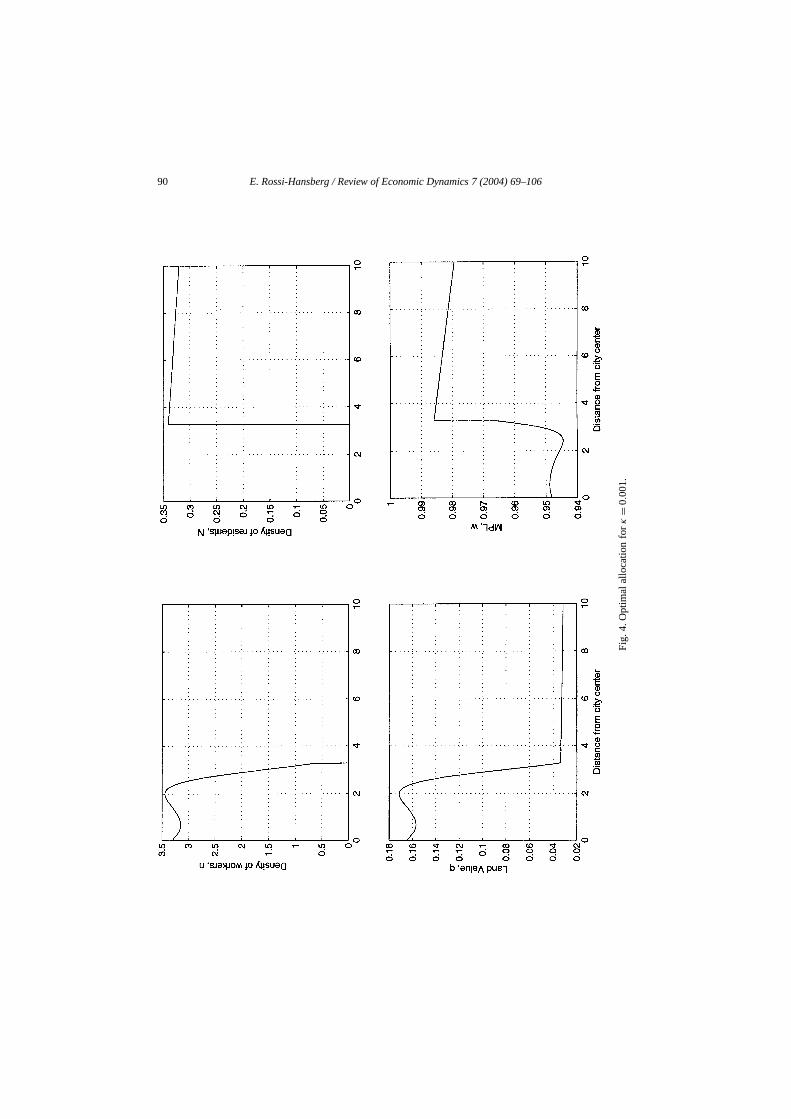
90 E. Rossi-Hansberg / Review of Economic Dynamics 7 (2004) 69–106
Fig
.4.O
ptim
alal
loca
tion
forκ
=0.
001
.
E. Rossi-Hansberg / Review of Economic Dynamics 7 (2004) 69–106 91
Fig
.5.O
ptim
alal
loca
tion
forκ
=0.
01.
92 E. Rossi-Hansberg / Review of Economic Dynamics 7 (2004) 69–106
e pureobtainption)y also
eases
sidentssidentsnd useat result, the
nlower
e
.
highery in alld
t is
lution
less wel like
h may
hefacedthe
business area of 2 miles. The rest of the city is residential. The exercise illustrates theffect of changes in land use on the density of workers. Endogenizing land use tooptimal employment densities is crucial. Net output (total output minus total consumincreases by 9.5%. One may argue that in order to evaluate this effect correctly it mabe important to look at the total number of residents in the city. This number incrby 10%.
Figure 6 shows the results of the same exercise forκ = 0.001 andκ = 0.01. In thesecases net output increases by 2.1% and 28% respectively. The total number of reincreases by 1.2% and 13%. The changes in net output and total number of resuggest that the higher commuting costs, the larger the effect of changes in the lastructure. Hence, the exercises suggest that zoning restrictions or labor subsidies thin equilibrium allocations that are similar to the optimal allocation imply a higher gainhigher commuting cost.
Another key parameter in the model is the externality parameterδ. A higherδ impliesthat the external effect decays faster with distance. Notice that a largerδ, as can be seein the equations presented in Section 2, does not imply that the external effect iseverywhere. This, since the functionϕ is also multiplied byδ. The idea is to make thexternal effect decay faster without changing the mean external effect.
In Fig. 7 we present the density of workers (multiplied byθ ) for δ = 5, 10, and 15A higher δ increases the amount of workers at the center whenκ = 0.001 and 0.005(the cases where there is a business district at the center). The intuition is that aδ increases the relative advantage of locating at the center, where firms are nearbdirections. Lucas (2001) provides some evidence of the need of highδs to fit Japanese lanrent data.
Notice that for allκ values used in the figure, a higherδ results in a business sector thamore concentrated. The intuition for this result is clear. A higherδ results in more localizedexternal effects and so, in order to take advantage of the externality, the optimal soyields a more concentrated business sector. For the case ofκ = 0.01, the concentrationof business areas may eventually lead to a business sector in the middle, neverthebelieve that values ofδ much higher than 15 are not reasonable for a one sector modethis.9 If we were to include different sectors, we may use a very largeδ for an industrylike financial services (see Dekle and Eaton, 1999, for some evidence on this), whicresult in this industry locating at the center.
5.1. Numerical results on optimal subsidies
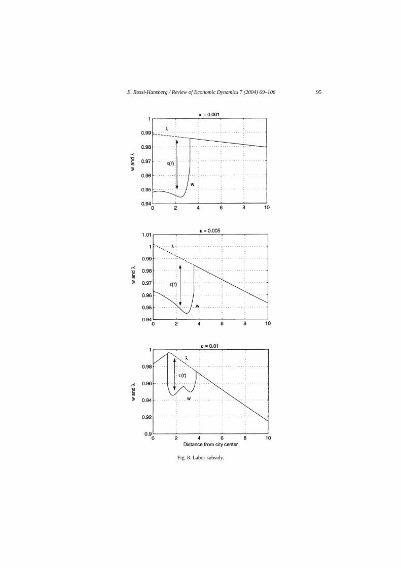
In Fig. 8, we present the optimal marginal product of labor and the functionλ for thedifferentκ values. The subsidyτ (r) is given by the difference between the two curves. Tsubsidy is never negative, it is actually a subsidy. The reason is that the externalityby firms is always positive, so in equilibrium they always hire less workers than inoptimum. The total subsidy -the area between the two curves- is larger the largerκ. This
9 If δ = 5, the external effect declines by half every 300 yards.

E. Rossi-Hansberg / Review of Economic Dynamics 7 (2004) 69–106 93
Fig. 6. Optimal density of workers.

94 E. Rossi-Hansberg / Review of Economic Dynamics 7 (2004) 69–106
Fig. 7. The effect ofδ.
E. Rossi-Hansberg / Review of Economic Dynamics 7 (2004) 69–106 95
Fig. 8. Labor subsidy.
96 E. Rossi-Hansberg / Review of Economic Dynamics 7 (2004) 69–106
hat the
d, thelandlower
result
oningericaltweent the
eter
ss netts. Thet theeasesation
grium.land
oundaryes ares that,effectmorelots arecond
ctivityty.
utinge city isreasee city
is true in absolute value but not as a percentage of total net output. We saw before tgains from this type of subsidy are larger, the largerκ.
There are two effects that determine the total bill of subsidies. On one hanhigherκ, the more important the difference between the equilibrium and optimumuse structure, which increases the total subsidy. On the other, the external effect isthe higherκ , and so the subsidy needed to internalize the externality is smaller. Theof this trade-off is the area depicted in these figures.
5.2. Numerical results on zoning restrictions
In Section 4, we discussed some of the theoretical implications of imposing zrestrictions. There are two important issues that we want to address using numexercises. The first is the extend in which zoning laws can reduce the difference beequilibrium and optimal net output. The second is the discontinuity of land rents aboundaries between business and residential areas.
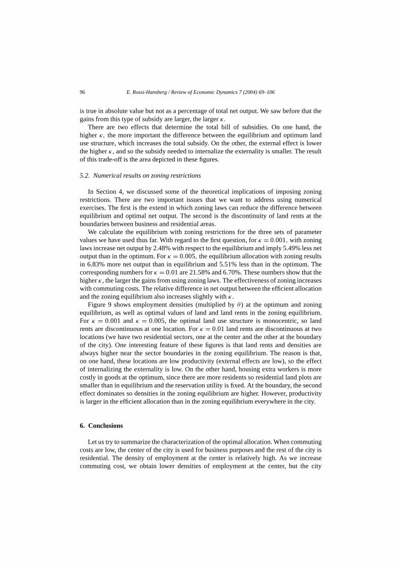
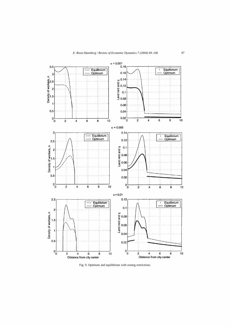
We calculate the equilibrium with zoning restrictions for the three sets of paramvalues we have used thus far. With regard to the first question, forκ = 0.001, with zoninglaws increase net output by 2.48% with respect to the equilibrium and imply 5.49% leoutput than in the optimum. Forκ = 0.005, the equilibrium allocation with zoning resulin 6.83% more net output than in equilibrium and 5.51% less than in the optimumcorresponding numbers forκ = 0.01 are 21.58% and 6.70%. These numbers show thahigherκ , the larger the gains from using zoning laws. The effectiveness of zoning incrwith commuting costs. The relative difference in net output between the efficient allocand the zoning equilibrium also increases slightly withκ .
Figure 9 shows employment densities (multiplied byθ ) at the optimum and zoninequilibrium, as well as optimal values of land and land rents in the zoning equilibFor κ = 0.001 andκ = 0.005, the optimal land use structure is monocentric, sorents are discontinuous at one location. Forκ = 0.01 land rents are discontinuous at twlocations (we have two residential sectors, one at the center and the other at the boof the city). One interesting feature of these figures is that land rents and densitialways higher near the sector boundaries in the zoning equilibrium. The reason ion one hand, these locations are low productivity (external effects are low), so theof internalizing the externality is low. On the other hand, housing extra workers iscostly in goods at the optimum, since there are more residents so residential land psmaller than in equilibrium and the reservation utility is fixed. At the boundary, the seeffect dominates so densities in the zoning equilibrium are higher. However, produis larger in the efficient allocation than in the zoning equilibrium everywhere in the ci
6. Conclusions
Let us try to summarize the characterization of the optimal allocation. When commcosts are low, the center of the city is used for business purposes and the rest of thresidential. The density of employment at the center is relatively high. As we inccommuting cost, we obtain lower densities of employment at the center, but th
E. Rossi-Hansberg / Review of Economic Dynamics 7 (2004) 69–106 97
Fig. 9. Optimum and equilibrium with zoning restrictions.

98 E. Rossi-Hansberg / Review of Economic Dynamics 7 (2004) 69–106
rea atreas. Inly a
ease,
s aserationin thisbuticies
In theence,
cordingsidents
ibriumthat,ixed
duction
se, ofntiallytheir
entedmumshow
ctions.on isse
our
iricals. Itolicyodeleyond
remains a Mills city. Further increases in commuting costs result in a residential athe center surrounded by a ring of business areas and then a ring of residential acontrast, in the equilibrium allocations presented in LRH, low commuting cost impMills city with high densities of employment at the center. As commuting costs incrthe center becomes mixed, with pure business and residential areas surrounding it.
Efficient and equilibrium allocations differ since we use production externalitiethe agglomeration force. Other theories in urban economics have proposed agglomeffects that are not external but internal to the firm. The allocations characterizedpaper can be viewed asequilibrium allocations of urban theories without externalitieswith agglomeration effects that take the form in (7). However, the validity of the polproposed does depend crucially on the presence of external effects.
Theorem 1 shows that there are no mixed areas in the efficient allocation.equilibrium allocation, however, there are mixed areas at the center of the city. Hwe should observe mixed areas in actual cities, but those areas are inefficient acto our model. Chicago is a good example of mixed areas at the center. Chicago recommuting by foot to work live mostly in downtown Chicago.
As we argued above, the results in this paper can be viewed as the equilallocation of a theory with internal agglomeration effects. Theorem 1 then impliesif agglomeration effects are internal to the firm, the equilibrium allocation has no mareas. Hence, the presence of mixed areas in actual cities is evidence of proexternalities.
The theory emphasizes that there is an indirect effect, via changes in land ureducing commuting costs. The numerical exercises show that the effect is poteimportant. City governments should try to include estimations of this gain inevaluation of projects and policies that reduce commuting costs.
Theorem 2 shows that using labor subsidies the optimal allocation can be implemas an equilibrium. Other policies like zoning restrictions do not implement the optibut do improve the production possibilities of a given city. The numerical exercisesthat zoning restriction are much more useful when commuting costs are high.
As Fig. 9 shows, land rents are discontinuous in the presence of zoning restriFirms would like to move to residential areas but they are not allowed. The reasthat optimal zoning restrictions alwaysconcentrate business areas in order to increaproductivity. Hence, with optimal zoning restrictions we know that firms, andnot residents,will have incentives to lobby for the elimination of zoning restrictions. Therefore,provides a test of the optimality of current regulation.
Given our focus on optimal allocations, our theory does not provide empimplications on land use structure. However, the parallel equilibrium theory doeis important to test the implications of our theory since we have made several precommendations. Their validity depends directly on the extent to which this mcaptures important elements of reality. A test of these implications is, nevertheless, bthe scope of this paper and left for future research.
E. Rossi-Hansberg / Review of Economic Dynamics 7 (2004) 69–106 99
vice.laumekoglursitys inthepaperodrigo
in theults are
ith
(ii)tiesatrian
there
lues,auder’s
thatelf and
Acknowledgments
I am particularly grateful to Robert E. Lucas Jr. for his support, guidance and adI also thank Fernando Alvarez, Marcus Berliant, Jan Brueckner, Jeff Campbell, GuilCarlier, Ivar Ekeland, Lars P. Hansen, Boyan Jovanovic, Nancy Stokey, Mehmet Yoruand seminar participants at Boston University, Brown University, UCSB, the Univeof Chicago, the University of Michigan, the Minneapolis FED, the SED MeetingStockholm, Stanford University, the University of Toronto, Vanderbilt University,editors of this journal, and an anonymous referee for helpful comments. Thebenefitted from discussions with Carlos da Costa, Claudio Irigoyen, Juan Santalo, RSoares, and Ivan Werning.
Appendix A. Proofs
In this appendix we prove all the theorems, propositions and lemmas not proveddifferent sections of the paper. The order is the same as the order in which the respresented in the text.
Proposition 1. Under Assumption A, given θ there exists a unique set of functions {n∗, N∗,c∗, �∗, z∗, H ∗, λ∗} that satisfies the first-order conditions and the Maximum Principleconditions.
Proof. Under Assumption A, givenθ, the problem is a strictly concave problem wconstraints that define a closed, convex and bounded set in{n∗, N∗, c∗, �∗, z∗, H ∗}.To see this, notice that, since the total amount of land is given by 2πS2, part (iii) ofAssumption A guarantees that 0< �(r) < 2πS2 and so thatc(r) is strictly positive andbounded.N(r) is then also strictly positive and bounded by (5). Assumption A parttogether with (6) result inn(r) strictly positive and bounded. Since all these properhold for everyr ∈ [0, S], they imply thatz(r) andH(r) are positive and bounded and ththe functionsn∗, N∗, c∗, �∗, z∗, H ∗ also inherit these properties. Hence by MangasaSufficiency Theorem there exists a unique solution to Problem (O), givenθ . The first-orderconditions and Maximum principle conditions are then necessary and sufficient, soexists a solution that satisfies them givenθ . ✷Proposition 2. Under Assumption A, there exists a function θ∗ such that T θ∗ = θ∗.
Proof. Since clearlyT does not have to be monotone for all sets of parameters vawe cannot base the proof on convergence of monotone operators. We will use Schfixed point theorem in the version proven in Zeidler (1986, Vol. 1). We need to provethe operatorT maps a nonempty, compact, convex subset of a Banach space into itsthatT is a continuous operator in that same space. For this, first define the spaceL1(R),a Lebesgue space, by the set of all measurable functionsf :R → R with ‖f ‖1<∞,where
‖f ‖1 =∫ ∣∣f (x)∣∣dx.
R

100 E. Rossi-Hansberg / Review of Economic Dynamics 7 (2004) 69–106
rly0.
.
onomin,
ssthat an
ss ofion.
).t
up-tion
Zeidler (1986, Vol. 1) provides a proof thatL1(R) is a Banach space, since cleathere are two functions, elements ofL1(R), that differ only by a set of measureNext, defineM as the set of all measurable functionsf : [0, S] → [0,1] with boundedvariation. Since‖f ‖1 < S <∞, M ⊂ L1(R), M is bounded andM is clearly nonemptyTo show thatM is convex, notice that forf1, f2 ∈M andα,β ∈ [0,1] with α + β = 1,0< αf1(x)+ βf2(x)≡ f3(x) < 1, all x ∈ [0, S]. Thus, since the set of bounded variatifunctions on a given interval is a linear space (see, for example, Kolmogorov and F1975),f3 ∈M.
We now prove thatM is a compact subset ofL1(R). For this we use the compactnetheorem of Riesz–Kolmogorov (see Zeidler, 1986, Vol. 2B). The theorem statesbounded subset ofL1(R) (say M) is relatively compact if and only if it is 1-meacontinuous, i.e., for eachε > 0, there exists aϑ(ε) > 0 such that
supu∈M
∫R
∣∣u(x + h)− u(x)∣∣dx < ε,
provided|h|< ϑ(ε). We setu(x)= 0 outsideS.We have shown thatM is a bounded subset ofL1(R). Notice that if the functionu that
achieves the supremum is continuous, the condition is trivially satisfied. Without logenerality assume that the functionu that achieves the supremum is an indicator functThen, if the number of discontinuity points inu is finite (sayD <∞),
supu∈M
∫R
∣∣u(x + h)− u(x)∣∣dx � hD < ε
for h < ε/D. If the number of discontinuity points is infinite, then the setSD at which|u(x+h)−u(x)| = 1 is of measure 0 sinceu has finite variation by Assumption A, part (vHenceM is relatively compact. Since both[0, S] and [0,1] are closed intervals, and losizes are bounded below by Assumption A, part (v), the setM is also closed and henceMis compact.T :M → M, follows from the definition ofT and the fact that ifθ has bounded
variation,λ andT are continuous and have bounded variation, which implies thatT θ hasbounded variation. Thus, the first set of conditions has been proven.
We now turn to the proof thatT is a continuous operator in‖ · ‖1. That is, we need toprove that if a sequence{θi}∞i=1 is such that
limi→∞
S∫0
∣∣θi(r)− θ(r)∣∣dr = 0,
it implies that
limi→∞
S∫0
∣∣T θi(r)− T θ(r)∣∣dr = 0.
In particular, because of the definition ofT , we need to show that ifθi(r)→ θ(r) in‖ · ‖1, λ(·; θi)→ λ(·; θ) andt (·; θi)→ t (·; θ) where this convergence can be in the snorm (‖ · ‖), (here we use a notation that emphasizes the dependence on the funcθ).
E. Rossi-Hansberg / Review of Economic Dynamics 7 (2004) 69–106 101
tor
m
or the
That is, we need to show thatλ and t are continuous inθ in ‖ · ‖. To show that this issufficient, notice that if this is the case,t − λ will be continuous and hence an indicafunction that is equal to 1 forr ’s such thatt (r)− λ(r)� 0 and equal to 0 forr ’s such thatt (r)− λ(r) > 0 will be continuous in‖ · ‖1. This, since ther ’s such thatt (r)− λ(r)= 0will change continuously withθ.
Showing thatλ and t are continuous inθ is equivalent to showing that the systeof first-order and Maximum Principle conditions forθi converge to the system forθ inthe sup-norm. We will do that by showing that all the terms that involveθ in the systemconverge.θ appears in three terms in the system, we will analyze each term in turn. Ffirst term,
∥∥∥∥∥S∫
0
sθi(s)g′(z(s; θi))f (
n(s; θi))ϕ(s, r)ds
−S∫
0
sθ(s)g′(z(s; θ))f (n(s; θ))ϕ(s, r)ds
∥∥∥∥∥� S2πδmax
s∈S[g′(max
[z(s; θi), z(s; θ)
])f
(max
[n(s; θi), n(s; θ)
])]
×∥∥∥∥∥
S∫0
[θi(s)− θ(s)
]ds
∥∥∥∥∥� S2πδmax
s∈S[g′(max
[z(s; θi), z(s; θ)
])f
(max
[n(s; θi), n(s; θ)
])]
×S∫
0
∣∣θi(s)− θ(s)∣∣ds,
where we are using the fact that for everyθ ∈ M, z(s; θ) andn(s; θ) are finite (see theproof of Proposition 1), thatϕ(s, r) ∈ [0,2πδ] ands � S.
For the second term,
∥∥∥∥∥S∫
0
ϕ(r, s)sθi(s)n(s; θi)ds −S∫
0
ϕ(r, s)sθ(s)n(s; θ)ds∥∥∥∥∥
� S2πδmax[n(s; θi), n(s; θ)
]∥∥∥∥∥S∫
0
[θi(s)− θ(s)
]ds
∥∥∥∥∥� S2πδmax
[n(s; θi), n(s; θ)
] S∫0
∣∣θi(s)− θ(s)∣∣ds.
For the third term, notice that
102 E. Rossi-Hansberg / Review of Economic Dynamics 7 (2004) 69–106
ll bye,
r and
-le).
danfo
easureions.
e
sups∈[0,S]
∣∣2πs[θi(s)n(s; θi)+ (1− θi(s)
)N(s; θi)
]− 2πs
[θi(s)n(s; θ)+
(1− θi(s)
)N(s; θi)
]∣∣� 2πs sup
s∈[0,S]max
[n(s; θi)− n(s; θ),N(s; θi)−N(s; θ)],
which does not involveθi or θ explicitly. So since the other two terms converge,n andN are continuous functions ofθ , and so the term above can be made arbitrarily smachoice ofi. Hencet andλ are continuous functions ofθ and so by the argument abovT is a continuous operator. Schauder’s fixed point theorem yields the result.✷Proposition 3. Under Assumption A, there exists a set of functions {θ∗, n∗,N∗, c∗, �∗, z∗,H ∗, λ∗} that satisfies the first-order conditions, the Maximum Principle conditions andT θ∗ = θ∗.
Proof. By Proposition 1, there exists a unique solution that satisfies the first-ordeMaximum Principle conditions givenθ . Proposition 2 shows the existence of aθ∗ suchthat T θ∗ = θ∗. Hence there exists a set of functions{θ∗, n∗,N∗, c∗, �∗, z∗,H ∗, λ∗} thatsatisfies all the necessary conditions for a maximum.✷Theorem 1. Under Assumption A, the optimal land use structure has no mixed areas. Thatis θ∗(r) ∈ {0,1}, except for sets with zero Lebesgue measure in [0, S].
Proof. For a mixed sector, we need
H(r)= 0, θ(r)n(r)− (1− θ(r)
)N(r)= 0, and t (r)= λ(r).
For anyr > 0 andε > 0 such thatH(r − ε) �= 0, given the value ofλ(r) and the valueof χ(r), plus the first-order condition with respect ton(r) andN(r), the system is overidentified (λ(r) follows one of the differential equations given by the Maximum PrincipThe reason is that we are imposing two extra conditions,H(r)= 0 andt (r)= λ(r). Thethird, θ(r)n(r)− (1 − θ(r))N(r) = 0 determinesθ(r). One condition could be satisfieby determining the valueλ(0) but we are still left with one condition. This equation cbe satisfiedonly for a given value ofλ(r) andχ(r), which implies that except for sets omeasure zero in the parameter space,t (r) = λ(r) or H(r)= 0 cannot be satisfied and smixed areas cannot be part of the solution. Notice that the argument above holdsonly formixed areas with positive Lebesgue measure, since for sets with zero Lebesgue mθ(r)n(r)− (1− θ(r))N(r)= 0 does not have to hold and so we loose one of the equat
There is a special case we still need to analyze. SinceH(0)= 0, by (6), it could be thecase that we start with a mixed area. Suppose thatr is a mixed area, in order for the threconditions above to hold,λ(r) will be determined byλ(r)= t (r). θ(r) is then given by
θ(r)= N(r)
N(r)+ n(r).
Notice that if λ(r) = t (r), the value ofL(r, θ(r) = 1) = L(r, θ(r) = 0) where L isthe Lagrangian evaluated at the maximizing values ofn,N, z, c, λ and H given θ.
E. Rossi-Hansberg / Review of Economic Dynamics 7 (2004) 69–106 103
on
ting
vex
elds
ssian
iseasure
Differentiatingλ(r) = t (r) with respect toθ(r) we obtain (omitting the dependencer in the notation)
∂2L(r, θ(r))
∂θ(r)2= g′(z)f (n) ∂z
∂θ+ n
∂χ
∂θ,
whereχ = χ/n and we used the first-order conditions to simplify the term. Differentiathe first-order condition with respect ton we obtain
g′(z)f ′(n) ∂z∂θ
+ g(z)f ′′(n)∂n∂θ
+ ∂χ
∂θ= 0, (A.1)
and substituting for∂χ/∂θ in the equation above we obtain that
∂2L(r, θ(r))
∂θ(r)2= g′(z)f (n)
[k
(n+ θ
∂n
∂θ
)][f (n)− nf ′(n)
] − g(z)f ′′(n)n∂n∂θ.
Where we used the fact that
∂z
∂θ=
[k
(n+ θ
∂n
∂θ
)], (A.2)
where k is a non-negative and continuous function ofr, with k(0) = 0. Notice that byAssumption A,f is strictly concave function and so the Lagrangian is a strictly confunction ofθ if
∂n
∂θ> 0.
Notice that sinceL(r, θ(r)= 1)= L(r, θ(r)= 0), this implies that
L(r, θ = 0,1) > L(r, θ ) for all θ ∈ (0,1).So the maximum of the Lagrangian is attained whenθ = 0 or 1, a contradiction with theassumption thatr was a mixed area. This, together with the first part of the proof, yithe result.
We still need to prove that∂n/∂θ > 0. For this notice that
∂χ
∂θ= k
[θg′′(z)f (n)
∂z
∂θ+ g′(z)f (n)+ θg′(z)f ′(z)
∂n
∂θ
].
Substituting this in (A.1) and using (A.2), we get
∂n
∂θ= k[g′(z)f (n)+ kθg′′(z)f (n)n]
−[θ2k2g′′(z)f (n)+ 2θ kg′(z)f ′(n)+ g(z)f ′′(z)] .
Notice that the term in brackets in the denominator is the quadratic form of the Heand by Assumption A is negative. Hence
∂n/∂θ > 0 if g′(z) >−kθg′′(z)n.
Since k(0) = 0 and k is continuous, forr sufficiently close to 0 the condition abovesatisfied. So it cannot be the case that we have a mixed area of positive Lebesgue mat the center.
104 E. Rossi-Hansberg / Review of Economic Dynamics 7 (2004) 69–106
s
983).the
of
ndin
Notice that ifg(·) is constant,∂n/∂θ = 0 for all θ ∈ [0,1] and if g(·) is linear thenthe condition above is clearly satisfied sinceg′′(z)= 0. A remark is that in the equilibriumcase in LRH since the agents do not controlz, ∂2L(r, θ(r))/∂θ(r)2 = 0 and so mixed areaare possible. ✷Proposition 4. Under Assumption A, there exists a set of functions {θ∗, n∗, N∗, c∗, �∗,z∗, H ∗, λ∗} that solves Problem (O).
Proof. We use relaxation theory to prove the Theorem (see Ekeland and Turnbull, 1Let L(r, θ(r), λ(r)) be the Lagrangian defined in Section 2.2 once we substitutefunctionsn,N, c, �, z, andH all as functions ofθ andλ. The existence and uniquenessthese functions is proven in Proposition 1. Let
L(r, θ(r), λ(r)
) ≡ minf : [0,S]×[0,1]×R→R
sup∣∣f (
r, θ(r), λ(r)) − L
(r, θ(r), λ(r)
)∣∣s.t. f
(r, θ(r), λ(r)
)� L
(r, θ(r), λ(r)
)and f
(r, ·, λ(r)) concave.
Then{x: x ∈ [
0, L(r, θ(r), λ(r)
)]for somer ∈ [0, S]}
is the convex hull of{x: x ∈ [
0, L(r, θ(r), λ(r)
)]for somer ∈ [0, S]}.
Hence, for everyr, there exists aθ(r) (maybe many) such that
θ (r)= argmaxθ
L(r, θ, λ(r)
).
Define
θ (r)= argmaxθ
L(r, θ, λ(r)
).
We need to show that for almost everyr, θ (r)= θ (r), since then
S∫0
L(r, θ (r), λ(r)
)dr =
S∫0
L(r, θ (r), λ(r)
)dr, (A.3)
and soθ (r) is a solution to Problem (O).If L(r,1, λ(r)) �= L(r,0, λ(r)), then L(r, θ, λ(r)) = L(r, θ, λ(r)) and soθ (r) = θ (r).
WhenL(r,1, λ(r))= L(r,0, λ(r)) and soL(r,1, λ(r))− L(r,0, λ(r)), the problem mayarise. It then implies thatθ(r) ⊆ [0,1] and may be a set with positive length. Hence, itmay be the case thatθ(r) �= θ (r). This is a problem ifL(r,1, λ(r)) = L(r,0, λ(r)) forsome set of positive Lebesgue measure since thenλ(s) �= λ(s), s > r, which results inθ (s) �= θ (s) for all s > r (whereλ(·) andλ(·) are the functions resulting fromθ(·) andθ (·)respectively).But since we showed in Theorem 1 thatL(r,1, λ(r))= L(r,0, λ(r)) only forsets of zero Lebesgue measure,θ (r) �= θ (r) only for sets of zero Lebesgue measure aso L(r, θ(r), λ(r)) �= L(r, θ (r), λ(r)) only for these sets. This implies that the equality(A.3) is satisfied. ✷
E. Rossi-Hansberg / Review of Economic Dynamics 7 (2004) 69–106 105
ond is
464.f Urban
onomic
mined
etation.
w 86,
Lemma 1. If U,f and g are Cobb–Douglas as specified above,
α,β, γ > 0, β,α < 1, and 1− α > γ,
then Assumption A is satisfied.
Proof. The result is obvious except for part (ii). We need to show that[ S∫0
ϕ(r, s)sθ(s)n(s)ds
]γn(r)α is concave inn
for anyθ. First notice that
z(r)=S∫
0
ϕ(r, s)sθ(s)n(s)ds is linear inn.
So we need to show that
Y (z,n)≡ zγ nα is concave inz andn.
The second and cross derivatives are given by:
∂2Y (z,n)
∂z2 = γ (γ − 1)zγ−2nα < 0,∂2Y (z,n)
∂n2 = α(α − 1)zγ nα−2< 0,
∂2Y (z,n)
∂n∂z= αγ zγ−1nα−1> 0.
The determinant of the Hessian is then given by
γ (γ − 1)α(α − 1)z2γ−2n2α−2 − α2γ 2z2γ−2n2α−21
= z2γ−2n2α−2(γ (γ − 1)α(α − 1)− α2γ 2) = z2γ−2n2α−2αγ (−γ − α + 1) > 0.
Hence the determinant of the first minor is negative and the determinant of the secpositive under the assumptions onα andγ in the statement. This implies thatY (z,n) isconcave inn andz and so part (ii) of Assumption A is satisfied.✷
References
Anas, A., Arnott, R., Small, K., 1998. Urban spatial structure. Journal of Economic Literature 36, 1426–1Anas, A., Xu, R., 1999. Congestion, land use, and job dispersion: a general equilibrium model. Journal o
Economics 45, 451–473.Berliant, M., Peng, S., Wang, P., 2002. Production externalities and urban configuration. Journal of Ec
Theory 104, 275–303.Borukhov, E., Hochman, O., 1977. Optimum and market equilibrium in a model of a city without a predeter
center. Environment and Planning A 9, 849–856.Caselli, F., Coleman II, W., 2001. The US structural transformation and regional convergence: a reinterpr
Journal of Political Economy 109, 584–616.Ciccone, A., Hall, R., 1996. Productivity and the density of economic activity. American Economic Revie
54–70.
106 E. Rossi-Hansberg / Review of Economic Dynamics 7 (2004) 69–106
. UPF
f Urban
ress,
proach.
gura-
y 100,
onomic
etrica 6,
denced
–1476.nomic
tions.
cities.
–272.ork.
Ciccone, A., Peri, G., 2002. Identifying human capital externalities: theory with an application to US citiesworking paper 661.
Dekle, R., Eaton, J., 1999. Agglomeration and land rents: evidence from the prefectures. Journal oEconomics 46, 200–214.
Dixit, A., 1973. The optimum factory town. Journal of Economics and Management 4, 637–651.Ekeland, I., Turnbull, T., 1983. Infinite-Dimensional Optimization and Convexity. Univ. of Chicago P
Chicago.Ellison, G., Glaeser, E.L., 1997. Geographic concentration in US manufacturing industries: a dartboard ap
Journal of Political Economy 105, 889–927.Fujita, M., Krugman, P., Venables, A., 1999. The Spatial Economy. MIT Press, Cambridge.Fujita, M., Ogawa, H., 1982. Multiple equilibria and structural transition of non-monocentric urban confi
tions. Regional Science and Urban Economics 12, 161–196.Fujita, M., Thisse, J., 2002. Economics of Agglomeration. Cambridge Univ. Press.Glaeser, E., Kallal, H., Scheinkman, J., Shleifer, A., 1992. Growth in cities. Journal of Political Econom
1126–1152.Henderson, V., 2001. Marschall’s scale economies. NBER working paper 7358.Helpman, E., Pines, D., 1977. Land use and zoning in an urban economy: further results. American Ec
Review 67, 982–986.Hochman, O., Pines, D., 1982. Adjustment costs and the spatial pattern of a growing open city. Econom
1371–1391.Jaffe, A.B., Trajtenberg, M., Henderson, R., 1993. Geographic localization of knowledge spillovers as evi
by patent citations. Quarterly Journal of Economics 63, 577–598.Kolmogorov, A., Fomin, S., 1975. Introductory Real Analysis. Dover, New York.Lucas, R.E. Jr., 2001. Externalities and cities. Review of Economic Dynamics 4, 245–267.Lucas, R.E. Jr., Rossi-Hansberg, E., 2002. On the internal structure of cities. Econometrica 70 (4), 1445Mills, E., 1967. An aggregate model of resource allocation in a metropolitan area. American Eco
Review 57, 197–210.Moretti, E., 2002. Human capital spillovers in manufacturing: evidence from plant-level production func
NBER working paper 9316.Rauch, J., 1993. Productivity gains from geographic concentration of human capital: evidence from the
Journal of Urban Economics 24, 380–400.Roback, J., 1982. Wages, rents, and quality of life. Journal of Political Economy 90, 1257–1278.Stull, W., 1974. Land use and zoning in an urban economy. American Economic Review 64, 337–347.Wheaton, W., 1998. Land use and density in cities with congestion. Journal of Urban Economics 43, 258Zeidler, E., 1986. Nonlinear Functional Analysis and its Applications. Vols. 1, 2B. Springer-Verlag, New Y