Optimal transportation betweenunequal dimensions∗

Robert J McCann† and Brendan Pass‡

Abstract

We establish that solving an optimal transportation problemin which the source and target densities are defined on spaceswith different dimensions, is equivalent to solving a new nonlo-cal analog of the Monge-Ampere equation, introduced here forthe first time. Under suitable topological conditions, we also es-tablish that solutions are smooth if and only if a local variantof the same equation admits a smooth and uniformly elliptic so-lution. We show that this local equation is elliptic, and C2,α

solutions can therefore be bootstrapped to obtain higher regu-larity results, assuming smoothness of the corresponding differ-ential operator, which we prove under simplifying assumptions.For one-dimensional targets, our sufficient criteria for regularityof solutions to the resulting ODE are considerably less restrictivethan those required by earlier works.

∗The authors are grateful to Toronto’s Fields’ Institute for the MathematicalSciences for its kind hospitality during part of this work, and to two anonymousreferees, for their careful reading and crucial comments. RJM acknowledges par-tial support of this research by Natural Sciences and Engineering Research Councilof Canada Grant 217006-15, by a Simons Foundation Fellowship, and by the USNational Science Foundation under Grant No. DMS-14401140 while in residence atthe Mathematical Sciences Research Institute in Berkeley CA during January andFebruary of 2016. He thanks S.-Y. Alice Chang for a stimulating conversation. BPis pleased to acknowledge support from Natural Sciences and Engineering ResearchCouncil of Canada Grants 412779-2012 and 04658-2018, as well as a University ofAlberta start-up grant. He is also grateful to the Pacific Institute for the Mathemat-ical Sciences, in Vancouver, BC, Canada, for its generous hospitality during his visitin February and March of 2017. c© by the authors, April 27, 2020†Department of Mathematics, University of Toronto, Toronto, Ontario, Canada

mccann@math.toronto.edu‡Department of Mathematical and Statistical Sciences, University of Alberta, Ed-

monton, Alberta, Canada pass@ualberta.ca.

1

1 Introduction

Since the 1980s [13] [26] [36] and the celebrated work of Brenier [2] [3],it has been well-understood [32] that for the quadratic cost c(x, y) =12|x− y|2 on Rn, solving the Monge-Kantorovich optimal transportation

problem is equivalent to solving a degenerate elliptic Monge-Ampereequation: that is, given two probability densities f and g on Rn, theunique optimal map between them, F = Du, is given by a convex solu-tion u to the boundary value problem

g ◦Du detD2u = f [a.e.], (1)

Du ∈ spt g [a.e.], (2)

where spt g ⊂ Rn is the smallest closed set of full mass for g. Simi-larly, its inverse is given by the gradient of the convex solution v to theboundary value problem

f ◦Dv detD2v = g [a.e.], (3)

Dv ∈ spt f [a.e.]. (4)

Notice the quadratic cost implicitly requires x and y to live in the samespace. Subsequent work of Ma, Trudinger and Wang [31] leads to ananalogous result for other cost functions c(x, y) = −s(x, y) satisfyingsuitable conditions, still requiring x and y to live in spaces of the samedimension n; see also earlier works such as [5] [21] [28] [33] [41]. Thepurpose of the present article is to explore what can be said when x ∈ Rm

and y ∈ Rn live in spaces with different dimensions m > n, as in e.g. [22][10] [30].

Although the symmetry between x and y is destroyed, the dualitytheorem from linear programming, [27] [37] [4], strongly suggests thatthe problem can still be reduced to finding a single scalar potential u(x)or v(y) reflecting the relative scarcity of supply f at x (or demand g aty). Although this potential solves a minimization problem, it is not clearwhat equation, if any, selects it. Nor whether one expects its solution tobe smoother than Lipschitz and semiconvex [21] [19]. These are amongthe questions addressed hereafter. Our primary results are as follows:We exhibit an integro-differential equation which selects v(y). In con-tradistinction to the case investigated by Ma, Trudinger and Wang, ourequation, though still fully nonlinear, is in general nonlocal. However,we also show this equation has two local analogs, one of which is at leastdegenerate-elliptic. These may or may not admit solutions: howeverunder mild topological conditions, it turns out they admit a C2 smooth,strongly elliptic solution if and only if the dual linear program admits C2

2

minimizers. These locality criteria build upon our results with Chiappori[10] from n = 1, and extend the notion of nestedness introduced thereto targets of arbitrary dimension. We also relax and refine the notion ofnestedness, leading to regularity results for a large new class of exam-ples even when n = 1. Our basic set-up is as follows. Fix m ≥ n ≥ 1and open sets X ⊂ Rm and Y ⊂ Rn equipped with Borel probabilitydensities f and g. We say F : X −→ Y pushes f forward to g = F#f ifF is Borel and ∫

Y

ψ(y)g(y)dy =

∫X

ψ(F (x))f(x)dx, (5)

for all bounded Borel test functions ψ ∈ L∞(Y ). If, in addition, Fhappens to be Lipschitz and its (n-dimensional) Jacobian JF (x) :=det1/2[DF (x)DF T (x)] vanishes at most on a set of f measure zero, thenthe co-area formula yields

g(y) =

∫F−1(y)

f(x)

JF (x)dHm−n(x) (6)

for a.e. y ∈ Y , where Hk denotes k-dimensional Hausdorff measure.Given a surplus function s ∈ C2(X × Y ), Monge’s problem is to

compute

s(f, g) := supF#f=g

∫X

s(x, F (x))f(x)dx, (7)

where the supremum is taken over maps F pushing f forward to g. Thesupremum is well-known to be uniquely attained provided X × Y isopen and s is twisted [40], meaning Dxs(x, ·) acts injectively on Y foreach x ∈ X; here Y denotes the closure of Y . It can be characterizedthrough the Kantorovich dual problem

s(f, g) = minu(x)+v(y)≥s(x,y)

∫X

u(x)f(x)dx+

∫Y

v(y)g(y)dy, (8)

where the minimum is taken over pairs (u, v) ∈ L1(f)⊕L1(g) satisfyingu⊕v ≥ s throughoutX×Y . Dual minimizers of the form (u, v) = (vs, us)are known to exist [40], where s(y, x) := s(x, y) and

vs(x) = supy∈Y

s(x, y)− v(y) us(y) = supx∈X

s(x, y)− u(x). (9)

Such pairs of payoff functions are called s-conjugate, and u and v aresaid to be s- and s-convex, respectively.

To motivate our first result, here and hereafter let

Y ⊂ Rn be open and bounded, X ⊂ Rm be open, m ≥ n (10)

and s ∈ C2(X × Y ) be twisted, non-degenerate, (11)

3

meaning in addition to the injectivity of y ∈ Y 7→ Dxs(x, y) men-tioned above that D2

xys(x, y) has maximal rank throughout X× Y . HereC2(X × Y ) denotes the usual Banach space. Suppose F maximizes theprimal problem (7) and (u, v) = (vs, us) is an s-conjugate pair of payoffsminimizing the dual problem (8). Then u(x) + v(y) − s(x, y) ≥ 0 onX × Y , with equality on graph(F ). Thus

F−1(y) ⊂ ∂sv(y) (12)

:= {x ∈ X | s(x, y)− v(y) = supy′∈Y

s(x, y′)− v(y′)}. (13)

Note that since Y is bounded, v must be bounded below — otherwiseu = vs ≡ +∞ and (u, v) cannot solve (8); this implies that u is locallyLipschitz as in [33, Lemma 1], hence the level set ∂sv(y) of x 7→ s(x, y)−u(x) is closed, a fortiori measurable. Since s ∈ C2(X×Y ), u and v admitsecond-order Taylor expansions Lebesgue a.e. as in e.g. [21] [40], andthe first- and second-order conditions for equality on graph(F ) imply

Dv(F (x)) =Dys(x, F (x)) [f -a.e.] and (14)

D2v(F (x))≥D2yys(x, F (x)) [f -a.e.]. (15)

Differentiating the first-order condition yields

[D2v(F (x))−D2yys(x, F (x))]DF (x) = D2

xys(x, F (x)) [f -a.e.] (16)

as in e.g. [31]. Since D2xys has full-rank, when F happens to be Lipschitz

we identify its Jacobian f -a.e. as

JF (x) =

√det[D2

xys(x, F (x))(D2xys(x, F (x)))T ]

det[D2v(F (x))−D2yys(x, F (x))]

. (17)

In this case we can rewrite (6) in the form

g(y) =

∫F−1(y)

det[D2v(y)−D2yys(x, y)]√

detD2xys(x, y)(D2

xys(x, y))Tf(x)dHm−n(x). (18)

Note that although we neither assume nor establish Lipschitz continuityof F in the sequel, for s ∈ C2 twisted the s-convexity of u makes Fcountably Lipschitz, as in e.g. Theorem 3.16 of [37].

Except for the appearance of the map F in the domain of integra-tion, this would be a partial differential equation relating v to the data(s, f, g). However, using twistedness of the surplus we’ll show that the

4

containment (12) is essentially saturated, in the sense that there ex-ists a certain set X(vs) ⊂ domD2vs of full Hm measure such that fora.e. y ∈ Y ,

g(y) =

∫∂sv(y)∩X(vs)

det(D2v(y)−D2yys(x, y))√

detD2xys(x, y)(D2

xys(x, y))Tf(x)dHm−n(x) [Hn-a.e.].

(19)Indeed, u = vs is known to be semiconvex, meaning there exists k ∈ Rsuch that u(x) + k|x|2 is convex on every ball B ⊂ X. Thus Du ∈BVloc(X), and §6.6.1–2 of [17] imply that for each positive integer i,there is a continuously differentiable map Hi on X with Hi = Du andDHi = D2u outside a set Zi of volume Hm[Zi] < 1/i. Moreover, we maytake Zi+1 ⊂ Zi and set X(vs) := (domD2vs) \ Z∞ where Z∞ := ∩i>0Zihas zero volume. Here domD2u denotes the subset of X where u admitsa second-order Taylor expansion.

Now (19) is an analog of the Monge-Ampere equation (1), familiarfrom the case s(x, y) = −1

2|x−y|2, or equivalently s(x, y) = x ·y. Notice

the boundary condition (2) for that case is automatically subsumed informulation (19). However, unlike the case m = n, it is badly nonlo-cal since the essential domain of integration ∂sv(y) defined in (12) maypotentially depend on v(y′) for all y′ ∈ Y .

For twisted non-degenerate s and an s-convex v, our first result statesthat v satisfies (19) if and only if v combines with its conjugate u = vs

to minimize (8); see Corollary 3 of §2. Since the optimal map F can berecovered from the first-order condition

Dxs(x, F (x)) = Du(x), (20)

analogous to (14), this shows Monge’s problem has been reduced to thesolution of the partial differential equation (19) for the s-convex scalarfunction v.

Although non-locality makes this equation a challenge to solve, itturns out there is a class of problems for which (19) can be replacedby a local partial differential equation, as follows. Introduce the m− ndimensional submanifold

X1(y, p,Q) :=X1(y, p) := {x ∈ X | Dys(x, y) = p}

of X and its closed subset

X2(y, p,Q) := {x ∈ X1(y, p) | D2yys(x, y) ≤ Q}. (21)

Now (14)–(15) imply

∂sv(y) ⊂ X2(y,Dv(y), D2v(y)) ⊂ X1(y,Dv(y)) (22)

5

for all y ∈ Y ∩ domD2v; here domD2v denotes the subset of Y wherev admits a second-order Taylor expansion. It is often the case that oneor both of these containments becomes an equality, at least up to Hm−n

negligible sets. In this case locality is restored: we can then write (19)in the form

G(y,Dv(y), D2v(y)) = g(y) [Hn-a.e. y ∈ Y ], (23)

where

G(y, p,Q) :=Gi(y, p,Q) (24)

:=

∫Xi(y,p,Q)

| det(Q−D2yys(x, y))|√

detD2xys(x, y)(D2

xys(x, y))Tf(x)dHm−n(x)

and either i = 1 or i = 2.Our second result states any classical s-convex solution v ∈ C2(Y ) to

either local problem (23) also solves the nonlocal one (19); Corollary 4.Assuming connectedness of Xi(y,Dv(y), D2v(y)), we show such a solu-tion exists in Theorem 6 of §3, if and only if the dual minimization (8)admits a C2 solution (vs, v = vss). For an n = 1 dimensional target,other necessary and sufficient conditions for the more restrictive varianti = 1 to admit an s-convex solution have been given in joint work withChiappori [10]. There the ordinary differential equation (23) is also ana-lyzed to show v inherits smoothness from suitable conditions on the data(s, f, g) in this so-called nested case. Although it is not be needed inwhat follows, we recall this definition for reference: when n = 1, (s, µ, ν)is said to be nested if for every y0 < y1 ∈ Y with

∫ y1y0g(y)dy > 0 we have

X≤(y0, k(y0)) ⊆ X<(y1, k(y1)), where

X≤(y, k) := {x ∈ X : Dys(x, y) ≤ k} =⋃p≤k

X1(y, p),

X<(y, k) := X≤(y, k) \ X1(y, k), and k(y) is defined as any solution ofthe proportional population splitting equation:∫

X≤(y,k(y))

f(x)dx =

∫ y

−∞g(z)dz.

In this case, we show in [10] that any anti-derivative v(y) =∫ yy0k(z)dz

of k is s-convex, (vs, v) minimizes (8), and that ∂sv(y) = X1(y, k(y)),so that v solves the i = 1 version of (23). It is therefore consistent totake the existence of a solution to (23) with i = 1 as the definition ofnestedness in higher dimensions (n > 1).

6

We go on to show that the operatorG2 is degenerate elliptic in §5, andthat the ellipticity is strict at points where G2 > 0. As a consequence, weare able to deduce higher regularity of solutions v of (23) with i = 2 fromC2,α regularity in Theorem 13, provided G2 is sufficiently smooth. InTheorem 14 of §6 we establish this smoothness for the simpler operatorG1, allowing for the passage from C2,α to higher regularity when G2 =G1. For one-dimensional targets, we establish the smoothness of G2 inTheorem 23 of §7, whether or not it coincides with G1. The hypothesizedsecond order smoothness and uniform ellipticity of v remain intriguingopen questions — with partial resolutions known only in the cases n = mof Ma, Trudinger and Wang [31] [38] (which built on earlier work ofCaffarelli [6] [7], Delanoe [16] and Urbas [39]), and for n = 1 in thenested case [10]; to these we now add the non-nested cases which satisfythe local equations (23)–(24) with (n, i) = (1, 2), resolved in §8 below.When regularity fails for m = n the size of the singular set has beenestimated by DePhilippis and Figalli [15], building on work of Figalli[18] with Kim [20]; for related results see Kitagawa and Kim [25] andthe survey [14].

Remark 1 (Boundedness of the domains) Throughout the rest ofthe paper Y ⊂ Rn is assumed bounded, while X ⊂ Rm is bounded fromSection 6 onwards. We define ∂X = ∅ when X = Rm. The source andtarget measures to be transported are assumed to be absolutely continu-ous with respect to Lebesgue, and given by densities f on X and g onY . The boundedness of domains is mainly assumed for simplicity; as isoften the case in optimal transport theory, we believe that many of theresults here can be established on unbounded domains with suitable decayassumptions on the measures. However, we expect that on unbounded do-mains the class of problems satisfying the local equations will be greatlyreduced, and in some cases trivial. To illustrate this expectation, weconsider the simplest and best understood case of unequal dimensionaloptimal transport, the theory corresponding to the i = 1 equation withone dimensional target (n = 1) from [10]. If s(x, y) = x · H(y) forsome curve H : Y ⊆ R → Rm, then the sets X1(y, p) are hyperplanesorthogonal to H ′(y). Therefore, if X = Rm, any two level sets X1(y, p)and X1(y′, p′) intersect in X unless H ′(y) and H ′(y′) are parallel. ByCorollary 5.6 in [10], the model cannot be nested for arbitrary f andg unless the direction of H ′(y) is constant; in this case, H(Y ) is con-tained in a line l and s(x, y) = xl ·H(y) (where xl is the projection of xonto l) takes the index form known to reduce the problem to a optimaltransport problem between the densities fl = (x 7→ xl)#f and g with onedimensional support.

7

On the other hand, when Y is unbounded the density g cannot have alower bound. In many cases, this precludes nestedness (see, for example,Theorem 3 in [35]).

2 A nonlocal partial differential equation for opti-mal transport

Given X ⊂ Rm and Y ⊂ Rn, a Borel probability density f on X anda Borel map F : X −→ Y , we define the pushed-forward measure ν :=F#f by ∫

Y

ψ(y)dν(y) =

∫X

ψ(F (x))f(x)dx (25)

for all bounded Borel functions ψ ∈ L∞(Y ). This definition extends (5)to the case where ν need not be absolutely continuous with respect toLebesgue; however when ν is absolutely continous with Lebesgue densityg, we abuse notation by writing g = F#f .

Recall s ∈ C2(X × Y ) is twisted if for each x ∈ X the map y ∈ Y 7→Dxs(x, y) is injective. If

Dxs(x, y) = p

we can then deduce y uniquely from x and p, in which case we writey = s-expx p := Dxs(x, ·)−1(p). The non-degeneracy (11) of s (full-rankof D2

xys) guarantees s-exp is a continuously differentiable function of(x, p) where defined, by the implicit function theorem. Thus for a twistedcost function, the first-order condition (20) allows us to identify the mapF = s-exp ◦Du at points of X where u happens to be differentiable. Wedenote the set of such points by domDu. Similarly we denote the set ofpoints where F : X −→ Y is approximately differentiable by domDF ,and the set where u admits a second order Taylor expansion by domD2u.When s is non-degenerate and twisted, (20) implies domDF = domD2u.

Theorem 2 (Properties of potential maps) Fix X ⊂ Rm, Y ⊂ Rn

and s as in (10)-(11). Any pair (u, v) = (vs, us) of s-conjugate functions(9) are semiconvex, Lipschitz, and have second-order Taylor expansionsLebesgue a.e. The map F : domDu −→ Y satisfying (20) is uniqueand differentiable Lebesgue a.e. Decompose Y into Y+ := Y ∩ domD2vand Y− = Y \ Y+ and set X± := F−1(Y±). The Jacobian JF (x) :=det1/2[DF (x)DF (x)T ] is positive on X+ ∩ domDF and given there by

JF (x) =

√det[D2

xys(x, F (x))D2xys(x, F (x))T ]

det[D2v(F (x))−D2yys(x, F (x))]

. (26)

8

Any Borel probability density on X can be decomposed as f = f++f−,where f± = f1X± are mutually singular. Their images F#(f±) are mea-sures living on the disjoint sets Y±. Here F#(f+) is absolutely continuouswith respect to Lebesgue: its density given by

g+(y) =

∫F−1(y)∩X(vs)

f+(x)

JF (x)dHm−n(x) [Hn-a.e. y ∈ Y ] (27)

=

∫∂sv(y)∩X(vs)

f+(x) det[D2v(y)−D2yys(x, y)]√

detD2xys(x, y)(D2

xys(x, y))TdHm−n(x), (28)

where X(vs) ⊂ domD2vs is the set defined after (19). If y ∈ Y + thenf+ = f on ∂sv(y)∩X(vs). Moreover, if F#(f−) is absolutely continuouswith respect to Lebesgue and assigns zero mass to ∂Y , then f = f+ in(27)–(28).

Proof. It is well-known that u = vs and v = us are Lipschitz andsemiconvex [34, Lemma 3.1]: they inherit distributional bounds such as|Du| ≤ supY |Dxs| and D2u ≥ infY D

2xxs from s ∈ C2 . This implies they

extend continuously to X and Y , where they are twice differentiable a.e.by Alexandrov’s theorem [40, Theorem 14.25]; indeed, for x0 ∈ domD2uwe have

0 = limx→x0

supp∈∂u(x)

p−Du(x0)−D2u(x0)(x− x0)

|x− x0|(29)

which asserts differentiability (rather than just approximate differentia-bility) of Du at x0.

Recall u(x) + v(y)− s(x, y) ≥ 0 on X × Y . For each x ∈ domDu atleast one y ∈ Y produces equality, since the maximum (9) defining vs(x)is attained. This y satisfies the first order condition Dxs(x, y) = Du(x),which identifies it as y = F (x) by the twist condition. We abbreviateF = s-exp ◦Du. We note Du is differentiable a.e. in a neighbourhood ofx ∈ domF , and the map s-exp is well-defined and continuously differen-tiable in a neighourhood of (x,Du(x)) by the twist and non-degeneracyof s. From the definition of X(vs) following (19), recall that for eachpositive integer i, there is a C1 smooth map Hi and set Zi of volumeHm[Zi] < 1/i, such that both Du = Hi and D2u = DHi hold outsideZi. Thus there is a map Fi ∈ C1(X, Y ) with F = Fi and DF = DFioutside Zi, which admits a Lipschitz extension (also denoted Fi) to allof Rm. As a result F is countably Lipschitz (and approximately dif-ferentiable Lebesgue a.e.); the fact that it is actually differentiable a.e.follows from s-exp ∈ C1 and (29). As remarked after (19), the setsZi+1 ⊂ Zi may be taken to be nested. We define Z∞ := ∩i>0Zi andX(vs) := domD2vs \ Z∞.

9

For each φ ∈ L1(Rm), the co-area formula [17, §3.4.3] asserts∫Rm

φ(x)JFi(x)dx =

∫Rn

dy

∫F−1i (y)

φdHm−n. (30)

If φ vanishes outside X \Zi we may drop the subscripts i in the formulaabove. Thus if Hm[Z] = 0 for any Z ⊂ X(vs), we conclude Hm−n[Z ∩F−1(y)] = 0 for almost all y ∈ Rn, and similary if Z ⊂ X(vs) is f -negligible, then Z ∩ F−1(y) is fdHm−n-negligible for almost all y ∈ Rn.

Since u(x) + v(y) − s(x, y) ≥ 0 vanishes at (x, F (x)) ∈ X × Y foreach x ∈ X+, we can differentiate (14) if x ∈ domDF to obtain (16).Since the right hand side has rank n we conclude both factors on theleft must have rank n as well. This shows JF (x) > 0 and noting (15)establishes (26).

Decomposing a probability density f = f+ + f− + f0 on X intof± = f1X± and f0 = 1X0 , where X0 := X \ DomDvs is Lebesguenegligible, the asserted mutual singularity follows from Y+ ∩ Y− = ∅ =X+ ∩ X−. Moreover, the bounded increasing sequence X+

i := {x ∈X+ \ Zi | |x| ≤ i, JF (x) > 1/i} of sets exhausts X+ \ Z∞. SettingX+

0 := ∅ and Xi := X+i \ X+

i−1 decomposes X+ \ Z∞ = ∪∞i=1Xi intocountably many disjoint Borel sets Xi ⊂ Rm on which F is C1 withJF (x) > 1/i on Xi. Set X∞ := X+ ∩ Z∞ and let fi = f+1Xi denote therestriction of f+ to Xi, and gi := F#fi the density of the push-forwardof fi. The absolute continuity of F#fi with respect to Lebesgue followssince JF (x) > 1/i on Xi. Given ψ ∈ L∞(Rn) with bounded supportensures φ = fiψ ◦ Fi/JFi ∈ L1(Rm) hence (30) implies∫

Rn

giψ=

∫Rm

fiψ ◦ Fi

=

∫Rn

dyψ(y)

∫Xi∩F−1

i (y)

fiJFi

dHm−n.

Recalling Fi = F and DFi = DF on Xi ⊂ X(vs), we infer

gi(y) =

∫F−1(y)∩X(vs)

fi(x)

JF (x)dHm−n(x). (31)

a.e. since ψ ∈ L∞ had bounded support but was otherwise arbitrary.Summing (31) on i, the disjointness of Xi yields 1X+ = 1X∞ +

∑1Xi ,

hence f+ = f∞ +∑fi and g+ =

∑gi. Since f∞ = 0 on X(vs), (27)

holds for Lebesgue a.e. y ∈ Y . By the monotone convergence theorem,g+ ∈ L1(Y , dHn) and has mass at most one; thus for a.e. y ∈ Y itsLebesgue density g+(y) is finite and implies finiteness of the integral in(27).

10

To establish (28), it suffices to observe (26) holds wherever f+ > 0and to verify F−1(y) = ∂sv(y) ∩ DomDvs. The containment ⊂ followsfrom (12), so we need only consider the reverse inclusion. Given x ∈∂sv(y) ∩ DomDvs, the twist condition (11) implies y = F (x), hencex ∈ F−1(y).

Now y ∈ Y+ implies f = f+ on F−1(y) ⊂ X+, hence on ∂sv(y)∩X(vs)by the previous sentence. If f chargesX\X+, both f− and F#f− are non-zero, in which case F#f− charges either ∂Y or the Lebesgue negligibleset Y \ domD2v which comprise Y−. When the latter possibilities areruled out by hypothesis, then f− = 0 a.e., implying f = f+ holds in(27)–(28).

Corollary 3 (Equivalence of optimal transport to nonlocal PDE)Under the hypotheses of Theorem 2, let f and g denote probability densi-ties on X and Y . If v = vss satisfies the nonlocal equation (19) [a.e. onY ], then (vs, v) minimize Kantorovich’s dual problem (8). Conversely,if (u, v) = (vs, us) minimize (8) then v satisfies (19) [a.e. on Y ].

Proof. First suppose v = vss satisfies the nonlocal PDE (19) on Y.Setting u = vs implies for each x ∈ domDu the inequality

u(x) + v(y)− s(x, y) ≥ 0 (32)

is saturated by some y ∈ Y . Identifying F (x) = y we have the first-order condition (20), whence F = s-exp ◦Du on domDu. We claim it isenough to show F#f = g: if so, integrating

u(x) + v(F (x)) = s(x, F (x))

against f yields ∫X

uf +

∫Y

vg =

∫X

s(x, F (x))f(x)dx,

which in turn shows F maximizes (7) and (u, v) minimizes (8) as desired.To establish F#f = g, comparing (19) with (28) yields g+ ≤ g on Y ,with equality holding throughout Y+ := Y ∩ domD2v. Since Y+ and Ydiffer by a Lebesgue negligible set, g+ = g is a probability measure. Thisimplies F#f− = 0, hence g = g+ = F#f as desired.

Conversely, suppose (u, v) = (vs, us) minimizes (8). Since twistednessof s implies (7) is attained, there is some map F : X −→ Y pushing fforward to g such that (32) becomes an equality f -a.e. on Graph(F ).This ensures F = s-exp ◦Du holds f -a.e. Since Y+ := Y ∩ domD2v is aset of full measure for g, we conclude X+ = F−1(Y+) has full measurefor f , whence f+ := f1X+ = f and g+ := F#(f+) = g. Now (19) followsfrom (28) as desired.

11

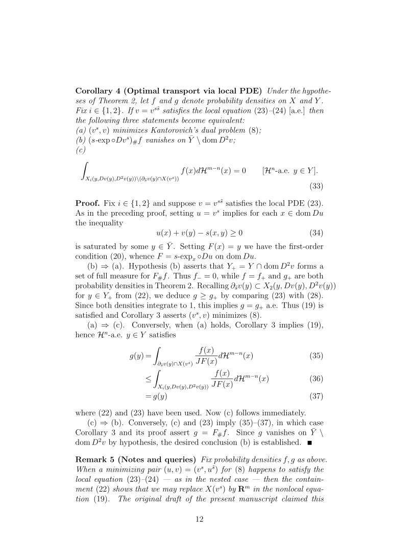
Corollary 4 (Optimal transport via local PDE) Under the hypothe-ses of Theorem 2, let f and g denote probability densities on X and Y .Fix i ∈ {1, 2}. If v = vss satisfies the local equation (23)–(24) [a.e.] thenthe following three statements become equivalent:(a) (vs, v) minimizes Kantorovich’s dual problem (8);(b) (s-exp ◦Dvs)#f vanishes on Y \ domD2v;(c)∫

Xi(y,Dv(y),D2v(y))\(∂sv(y)∩X(vs))

f(x)dHm−n(x) = 0 [Hn-a.e. y ∈ Y ].

(33)

Proof. Fix i ∈ {1, 2} and suppose v = vss satisfies the local PDE (23).As in the preceding proof, setting u = vs implies for each x ∈ domDuthe inequality

u(x) + v(y)− s(x, y) ≥ 0 (34)

is saturated by some y ∈ Y . Setting F (x) = y we have the first-ordercondition (20), whence F = s-expx ◦Du on domDu.

(b) ⇒ (a). Hypothesis (b) asserts that Y+ = Y ∩ domD2v forms aset of full measure for F#f . Thus f− = 0, while f = f+ and g+ are bothprobability densities in Theorem 2. Recalling ∂sv(y) ⊂ X2(y,Dv(y), D2v(y))for y ∈ Y+ from (22), we deduce g ≥ g+ by comparing (23) with (28).Since both densities integrate to 1, this implies g = g+ a.e. Thus (19) issatisfied and Corollary 3 asserts (vs, v) minimizes (8).

(a) ⇒ (c). Conversely, when (a) holds, Corollary 3 implies (19),hence Hn-a.e. y ∈ Y satisfies

g(y) =

∫∂sv(y)∩X(vs)

f(x)

JF (x)dHm−n(x) (35)

≤∫Xi(y,Dv(y),D2v(y))

f(x)

JF (x)dHm−n(x) (36)

= g(y) (37)

where (22) and (23) have been used. Now (c) follows immediately.(c) ⇒ (b). Conversely, (c) and (23) imply (35)–(37), in which case

Corollary 3 and its proof assert g = F#f . Since g vanishes on Y \domD2v by hypothesis, the desired conclusion (b) is established.

Remark 5 (Notes and queries) Fix probability densities f, g as above.When a minimizing pair (u, v) = (vs, us) for (8) happens to satisfy thelocal equation (23)–(24) — as in the nested case — then the contain-ment (22) shows that we may replace X(vs) by Rm in the nonlocal equa-tion (19). The original draft of the present manuscript claimed this

12

was true more generally, but our argument there suffered from a gap(which we would be glad to know how to close): although X \ X(vs)is Hm-negligible, we cannot be sure that its intersection with ∂sv(y) isHm−n-negligible for Hn-a.e. y ∈ Y — unless the map F (x) = s-expDvs

happens to be Lipschitz instead of countably Lipschitz.When m = n and both s and s(y, x) = s(x, y) are twisted, it follows

e.g. from Theorem 11.1 of [40] that any minimizing pair (u, v) = (vs, us)satisfies the local equation with i = 1. If, in addition, s satisfies Ma-Trudinger-Wang condition (A3w) of [31] [38], the converse can be shown:if v = vss solves the i = 1 local equation a.e. then (vs, v) minimizes (8).(Here (A3w) is to deduce a.e. injectivity of F from JF (x) > 0, using theconnectedness of ∂su(x) shown by Loeper [29].) In this case (a) followsfrom the other hypotheses of Corollary 4. We don’t know whether or notthe conditions (a)-(c) are similarly redundant under weaker hypotheses,as when m > n. If not, then:

Since (b) holds whenever v ∈ C2(Y ), it might conceivably turn outto be a criterion for selecting (i.e. or defining) an appropriate notion ofweak solution among nonsmooth functions v = vss satisfying (23)–(24).

3 Local PDE from optimal transport

As a partial converse to the preceding corollary, we assert that for ei-ther the more restrictive (i = 1) or less restrictive (i = 2) local partialdifferential equation (23) to admit solutions, it is sufficient that the Kan-torovich dual problem admit a smooth minimizer (u, v), with connectedpotential indifference sets Xi(y,Dv(y), D2v(y)) — in which case v alsosolves (23).

Theorem 6 (When a smooth minimizer implies nestedness) Fixs and probability densities f and g on X ⊂ Rm and Y ⊂ Rn as in (10)–(11). Let i ∈ {1, 2}. If (u, v) = (vs, us) ∈ C2(X)×C2(Y ) minimizes theKantorovich dual (8) then equation (23) holds Hn-a.e. on any measurableY ′ ⊂ Y having Xi(y,Dv(y), D2v(y)) connected for all y ∈ Y ′.

The assumed smoothness of u and v is essential. When the dualproblem (8) has no smooth optimizers, Remark 5 shows the local equa-tion (23) cannot have smooth c-convex solutions, neither for i = 2 norfor i = 1. For example, the explicit solution computed with Chiapporiin Section 3.3.3 of [9] solves the non-local equation (19) but neither localversion (23). Conversely, having solutions to either local equation willoften imply smoothness of v, as in the nested case [10] when n = 1 andi = 1, and the last section of the present paper when n = 1 and i = 2.It is quite possible, however, for smooth solutions v to the i = 2 localequation to produce non-smooth u = vs, as Example 8 below illustrates.

13

Proof. Corollary 3 implies v solves the non-local equation (19) a.e.,with X(vs) = X since u ∈ C2(X) by hypothesis. The local equationG = g follows wherever we have equality in the inclusion

∂sv(y) ⊂ Xi(y,Dv(y), D2v(y)). (38)

We now derive this equality for all y′ ∈ Y with ∂sv(y′) non-empty andX ′i := Xi(y

′, Dv(y′), D2v(y′)) connected.Observe both ∂sv(y′) and X ′i are relatively closed subsets of X. Thus

∂sv(y′) is also closed relative to X ′i. To show it is relatively open, letx′ ∈ ∂sv(y′). Since u, v ∈ C2 we see F ∈ C1(X) and DF has full rankat x′. By the Local Submersion Theorem [23], this means we can find aC1 coordinate chart on a neighbourhood U ⊂ X of x′ in which F actsas the canonical submersion: F (x1, . . . , xn, xn+1, . . . , xm) = (x1, . . . , xn).In these coordinates,

[{y′} ×Rm−n] ∩ U = F−1(y′) ∩ U ⊂ ∂sv(y′) ∩ U ⊂ X ′i ∩ U ⊂ X ′1 ∩ U

follows from (38). But Proposition 3.2 of [10] shows X ′1 to be an m− ndimensional submanifold of X, so equality must hold in this chain ofinclusions (at least if U is a ball in the new coordinates). This showsx′ lies in the interior of ∂sv(y′) relative to X ′i, concluding the proofthat ∂sv(y′) is relatively open. Thus ∂sv(y′) = X ′i since the former isopen, closed and non-empty and the latter is connected. Equality in(38) has been established whenever Xi(y,Dv(y), D2v(y)) is connected,concluding the proof.

The following example shows that the level set connectivity assump-tion in the preceding theorem is required to deduce that smooth solutionsto the dual problem solve the local equation; it also illustrates why itmay be necessary to consider the i = 2 case. In the example, the smooths-conjugate dual potentials (u, v) solve the i = 2 but not i = 1 equation;note that each X2(y,Dv(y), D2v(y)) = ∂sv(y) is connected whereas eachX1(y,Dv(y)) has two connected components — one is a segment on aray through the origin and the other its negation.

Example 7 (Annulus to circle) Consider transporting uniform masson the annulus, X = {x ∈ R2 : 1/2 ≤ |x| ≤ 1} to uniform measureon the punctured circle, C = {(−1, 0) 6= y ∈ R2 : |y| = 1} with thebilinear surplus, x · y. It is easy to see that x · y ≤ |x|, with equalityonly when y = x

|x| , implying that the optimal map takes the form x ∈X 7→ x

|x| ∈ C has a convex potential u(x) = |x| which is smooth on the

annulus X. Parameterizing C by y(θ) = (cos(θ) sin(θ)) for θ ∈ Y :=(−π, π) places this problem within our framework. In these coordinates,

14

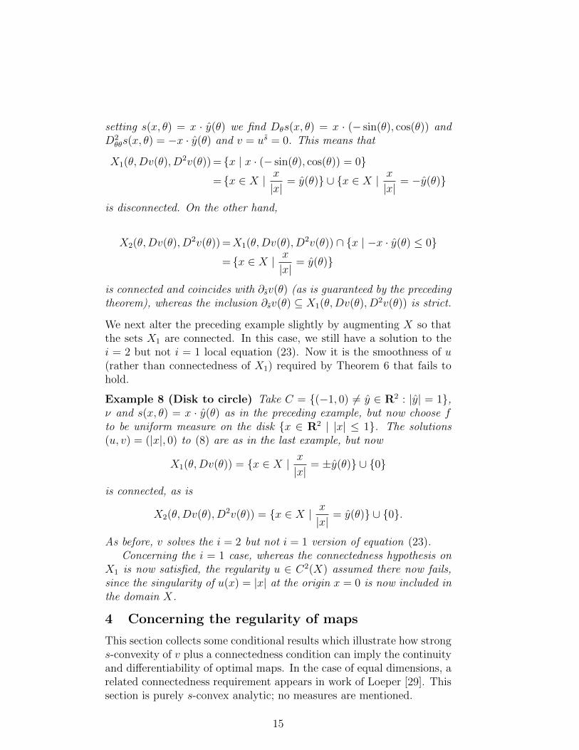
setting s(x, θ) = x · y(θ) we find Dθs(x, θ) = x · (− sin(θ), cos(θ)) andD2θθs(x, θ) = −x · y(θ) and v = us = 0. This means that

X1(θ,Dv(θ), D2v(θ)) = {x | x · (− sin(θ), cos(θ)) = 0}= {x ∈ X | x

|x|= y(θ)} ∪ {x ∈ X | x

|x|= −y(θ)}

is disconnected. On the other hand,

X2(θ,Dv(θ), D2v(θ)) =X1(θ,Dv(θ), D2v(θ)) ∩ {x | −x · y(θ) ≤ 0}= {x ∈ X | x

|x|= y(θ)}

is connected and coincides with ∂sv(θ) (as is guaranteed by the precedingtheorem), whereas the inclusion ∂sv(θ) ⊆ X1(θ,Dv(θ), D2v(θ)) is strict.

We next alter the preceding example slightly by augmenting X so thatthe sets X1 are connected. In this case, we still have a solution to thei = 2 but not i = 1 local equation (23). Now it is the smoothness of u(rather than connectedness of X1) required by Theorem 6 that fails tohold.

Example 8 (Disk to circle) Take C = {(−1, 0) 6= y ∈ R2 : |y| = 1},ν and s(x, θ) = x · y(θ) as in the preceding example, but now choose fto be uniform measure on the disk {x ∈ R2 | |x| ≤ 1}. The solutions(u, v) = (|x|, 0) to (8) are as in the last example, but now

X1(θ,Dv(θ)) = {x ∈ X | x|x|

= ±y(θ)} ∪ {0}

is connected, as is

X2(θ,Dv(θ), D2v(θ)) = {x ∈ X | x|x|

= y(θ)} ∪ {0}.

As before, v solves the i = 2 but not i = 1 version of equation (23).Concerning the i = 1 case, whereas the connectedness hypothesis on

X1 is now satisfied, the regularity u ∈ C2(X) assumed there now fails,since the singularity of u(x) = |x| at the origin x = 0 is now included inthe domain X.

4 Concerning the regularity of maps

This section collects some conditional results which illustrate how strongs-convexity of v plus a connectedness condition can imply the continuityand differentiability of optimal maps. In the case of equal dimensions, arelated connectedness requirement appears in work of Loeper [29]. Thissection is purely s-convex analytic; no measures are mentioned.

15

Lemma 9 (Continuity of maps (local)) Fix X, Y and s as in (10)–(11). Let (u, v) = (vs, us) and D2v(y) > D2

yys(x, y) for some (x, y) ∈X × [Y ∩∂svs(x) ∩ domD2v]. Then any C1 curve in ∂su(x) passingthrough y is constant; in particular, if ∂su(x) is C1-path-connected thenx ∈ domDu.

Proof. Fix (u, v) and (x, y) as in the lemma. The proof is by contra-diction; if the lemma is false, then there exists a continuously differen-tiable curve y : t ∈ [0, 1] 7→ y(t) ∈ ∂su(x) departing from y(0) = ywith non-zero velocity y′(0) 6= 0. Since the non-negative functionu(x) + v(·) − s(x, ·) ≥ 0 vanishes on this curve, differentiation showsy′(0) to be in the nullspace of D2v(y)−D2

yys(x, y). This contradicts thepositive-definiteness assertion and shows no such curve can exist.

Thus C1-path connectedness implies ∂su(x) = {y}. The semicon-vexity of u shown in Theorem 2 implies x ∈ domDu provided we canestablish convergence ofDu(xk) to a unique limit whenever xk ∈ domDuconverges to x. Therefore, let xk ∈ domDu converge to x, and chooseyk ∈ ∂su(xk). Any accumulation point y∞ of the yk satisfies y∞ ∈∂su(x) = {y}. Now letting k → ∞ in Du(xk) = Dxs(xk, yk) yieldsDu(xk)→ Dxs(x, y) to establish x ∈ domDu.

Corollary 10 (Continuity of maps (global)) Fix X, Y and s as in(10)–(11). Let (u, v) = (vs, us) with v ∈ C2(Y ). Then u ∈ C1(X) if foreach x ∈ X: ∂su(x) is C1-path connected and D2v(y) > D2

yys(x, y) forsome y ∈ Y ∩ ∂su(x) ∩ domD2v.

Proof. Lemma 9 implies X = domDu under the hypotheses of Corol-lary 10. Since semiconvexity of u was shown in Theorem 2, this issufficient to conclude u ∈ C1(X).

Proposition 11 (Criteria for differentiability of maps) Fix X, Yand s as in (10)–(11). Use (u, v) = (vs, us) with u ∈ C1(X) to defineF : X −→ Y through (20). Then both F and D2

xys(·, F (·)) are in (BVloc∩C)(X,Rn). If, in addition, v ∈ C1,1(Y ) then F (x) ∈ DomD2v for all xin a set of |DF | full measure, and as measures

(D2v(F (x))−D2yys(x, F (x)))DF (x) = D2

xys(x, F (x)). (39)

In this case, F is Lipschitz in any open subset Z of X admitting ε > 0for which

D2v(F (x))−D2yys(x, F (x)) ≥ εI (40)

holds for all x ∈ Z; (moreover, F inherits higher differentiability from vand s in this case).

16

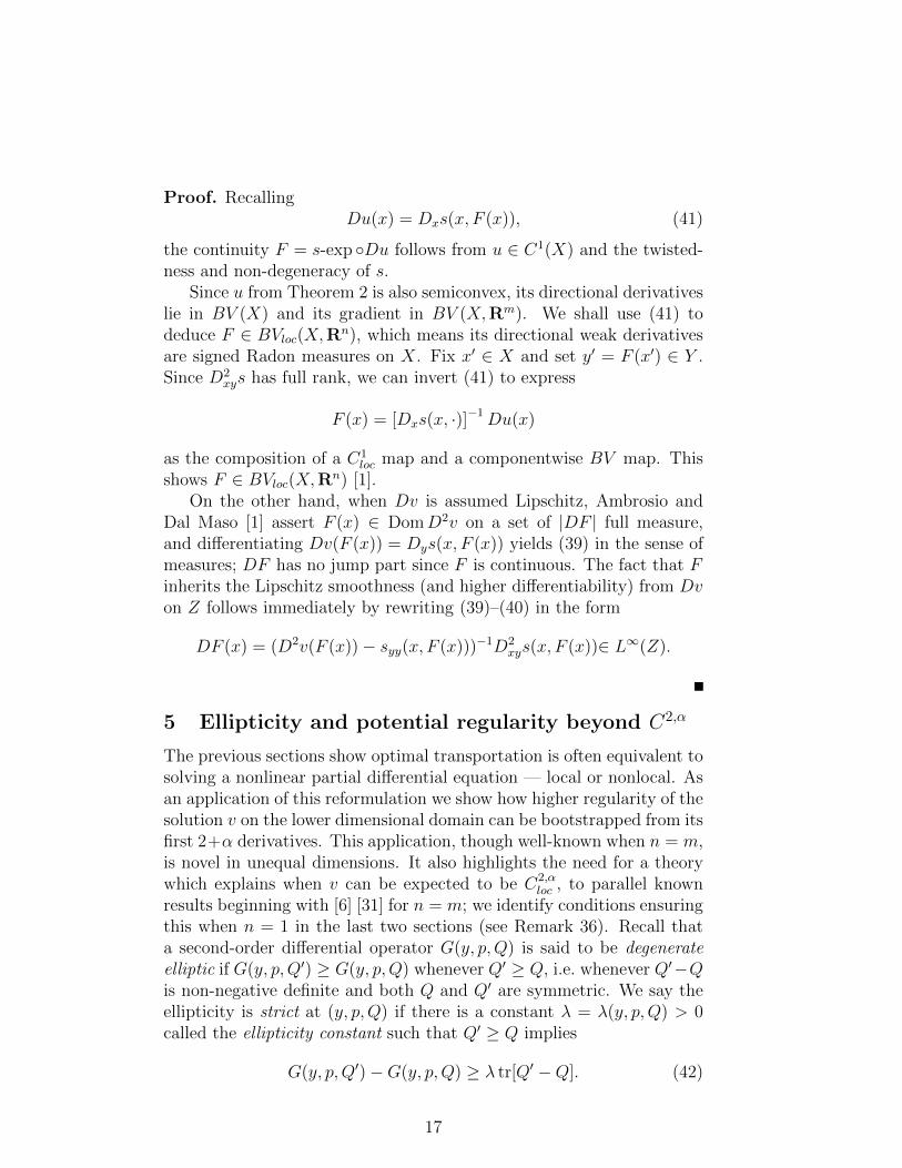
Proof. RecallingDu(x) = Dxs(x, F (x)), (41)

the continuity F = s-exp ◦Du follows from u ∈ C1(X) and the twisted-ness and non-degeneracy of s.

Since u from Theorem 2 is also semiconvex, its directional derivativeslie in BV (X) and its gradient in BV (X,Rm). We shall use (41) todeduce F ∈ BVloc(X,Rn), which means its directional weak derivativesare signed Radon measures on X. Fix x′ ∈ X and set y′ = F (x′) ∈ Y .Since D2

xys has full rank, we can invert (41) to express

F (x) = [Dxs(x, ·)]−1Du(x)

as the composition of a C1loc map and a componentwise BV map. This

shows F ∈ BVloc(X,Rn) [1].On the other hand, when Dv is assumed Lipschitz, Ambrosio and

Dal Maso [1] assert F (x) ∈ DomD2v on a set of |DF | full measure,and differentiating Dv(F (x)) = Dys(x, F (x)) yields (39) in the sense ofmeasures; DF has no jump part since F is continuous. The fact that Finherits the Lipschitz smoothness (and higher differentiability) from Dvon Z follows immediately by rewriting (39)–(40) in the form

DF (x) = (D2v(F (x))− syy(x, F (x)))−1D2xys(x, F (x))∈ L∞(Z).

5 Ellipticity and potential regularity beyond C2,α

The previous sections show optimal transportation is often equivalent tosolving a nonlinear partial differential equation — local or nonlocal. Asan application of this reformulation we show how higher regularity of thesolution v on the lower dimensional domain can be bootstrapped from itsfirst 2+α derivatives. This application, though well-known when n = m,is novel in unequal dimensions. It also highlights the need for a theorywhich explains when v can be expected to be C2,α

loc , to parallel knownresults beginning with [6] [31] for n = m; we identify conditions ensuringthis when n = 1 in the last two sections (see Remark 36). Recall thata second-order differential operator G(y, p,Q) is said to be degenerateelliptic if G(y, p,Q′) ≥ G(y, p,Q) whenever Q′ ≥ Q, i.e. whenever Q′−Qis non-negative definite and both Q and Q′ are symmetric. We say theellipticity is strict at (y, p,Q) if there is a constant λ = λ(y, p,Q) > 0called the ellipticity constant such that Q′ ≥ Q implies

G(y, p,Q′)−G(y, p,Q) ≥ λ tr[Q′ −Q]. (42)

17

Note that for C1 operators G, ellipticity is equivalent to everywhere

positive semi-definiteness of the matrix(

∂G∂Qij

). Uniform positive def-

initeness implies strict ellipticity; any lower bound λ on(

∂G∂Qij

)is an

ellipticity constant.

Lemma 12 (Strict ellipticity) Fix X, Y and s as in (10)–(11). Theoperator G defined by (21) and (24) with i = 2 is degenerate elliptic.Moreover, if G(y, p,Q) > 0, and there exists Θ > 0 such that Q −D2yys(x, y) ≤ ΘI for all x ∈ X2(y, p,Q), then the ellipticity constant of

G at (y, p,Q) is given by λ = G(y, p,Q)/Θ.

Proof. Fixing (y, p) ∈ Y ×Rm and m×m symmetric matrices Q′ ≥ Q,degenerate ellipticity ofG follows from the facts that f ≥ 0, X2(y, p,Q) ⊂X2(y, p,Q′), and Q′ − D2

yys(x, y) ≥ Q − D2yys(x, y) ≥ 0 for all x ∈

X2(y, p,Q).Now suppose also Q−D2

yys(x, y) ≤ ΘI <∞ for all x ∈ X2(y, p,Q),so that the product ((Q−D2

yys(x, y))−1−Θ−1I)(Q′−Q) of non-negativedefinite matrices has all non-negative eigenvalues, and therefore,

tr[(Q−D2yys(x, y))−1(Q′ −Q)] ≥ Θ−1tr[Q′ −Q]

for all Q′ ≥ Q. From here, letting λi ≥ 0 denote the eigenvalues of(Q−D2

yys(x, y))−1(Q′ −Q) we deduce

det[I + (Q−D2yys)

−1(Q′ −Q)] = Πni=1(1 + λi)

≥ 1 +n∑i=1

λi

= 1 + tr[(Q−D2yys(x, y))−1(Q′ −Q)]

≥ 1 + Θ−1tr[Q′ −Q].

This can be integrated against det[Q−D2yys]fdHm−n/ det[D2

xysD2xys

T ]over X2(y, p,Q) to find

G(y, p,Q′)

G(y, p,Q)≥ 1 + Θ−1tr[Q′ −Q].

as desired.

Theorem 13 (Bootstrapping regularity using Schauder theory)Fix 0 < α < 1, an integer k ≥ 2, and X, Y and s as in (10)–(11). Ifg > ε > 0 on some smooth domain Y ′ compactly contained in Y ⊂ Rn

where v ∈ Ck,α(Y ′), and G − g ∈ Ck−1,α in a neighbourhood N of the2-jet of v over Y ′, then (23)–(24) with i = 2 implies v ∈ Ck+1,α(Y ′).

18

Proof. Since v ∈ C2,α(Y ′), (23) holds in the classical sense. If k ≥ 3,we can differentiate the equation in (say) the ek direction to obtain alinear second-order elliptic equation

aij(y)D2ijw + bi(y)Diw = d(y) (43)

for w = ∂v/∂yk whose coefficients

aij(y) :=∂G

∂Qij

∣∣∣∣(y,Dv(y),D2v(y))

bi(y) :=∂G

∂pi

∣∣∣∣(y,Dv(y),D2v(y))

and inhomogeneity

d(y) =∂g

∂yk

∣∣∣∣y

− ∂G

∂yk

∣∣∣∣(y,Dv(y),D2v(y))

have (i) Ck−2,α2norm controlled by ‖G− g‖Ck−1,α‖v‖αCk,α and (ii) Ck−2,α

norm controlled by ‖G − g‖Ck−1,α‖v‖Ck,1 . In case k = 2, we shall ar-gue below that w ∈ C1,α solves (43) in the viscosity sense described e.g.in [12]. From Lemma 12 we see the matrix (aij) is bounded below byεI/‖v−s‖C2(X×Y ′); it is bounded above by ‖G‖C1(N). Thus the equationsatisfied by w on Y ′ is uniformly elliptic. Since the coefficient of w van-ishes in (43), the Dirichlet problem with continuous boundary data onany ball in Y ′ is known to admit a unique (viscosity) solution [12]; more-

over, this solution is (i) Ck,α2

loc (by e.g. Gilbarg & Trudinger Theorems

6.13 (k = 2) or 6.17 (k > 2). Thus we infer v ∈ Ck+1,α2

loc (Y ′). Apply-ing the same argument again starting from the improved estimates (ii)now established yields v ∈ Ck+1,α

loc (Y ′). At this point we have gained thedesired derivative of smoothness for v; starting from a neighbourhoodslightly larger than Y ′ yields v ∈ Ck+1,α(Y ′).

In case k = 2, applying the finite difference operator ∆hkv(y) :=

[v(y + hek) − v(y)]/h to the equation (23), the mean value theoremyields h∗(y) ∈ [0, h] lower semicontinuous such that

0 = ∆hk[G(y,Dv(y), D2v(y))− g(y)]

= aijh (y)D2ijwh + bih(y)Diwh − dh(y).

19

Here wh = ∆hkv and the coefficients

aijh (y) :=∂G

∂Qij

∣∣∣∣(I+h∗(y)∆h

k)(y,Dv(y),D2v(y))

bih(y) :=∂G

∂pi

∣∣∣∣(I+h∗(y)∆h

k)(y,Dv(y),D2v(y))

dh(y) =∂g

∂yk

∣∣∣∣y+h∗(y)ek

− ∂G

∂yk

∣∣∣∣(I+h∗(y)∆h

k)(y,Dv(y),D2v(y))

.

are measurable and converge uniformly to (aij, bi, d) as h → 0. The so-lutions wh = ∆h

kv ∈ C2,α, being finite differences, converge to ∂v/∂yk inC1,α(Y ′). Lemma 6.1 and Remark 6.3 of [12] show this partial derivativew = ∂v/∂yk must then be the required viscosity solution of the limitingequation (43).

Notice G2 is degenerate elliptic even when evaluated on functionswhich are not s-convex.

6 On smoothness of the nonlinear operators Gi

The preceding section illustrates how one can bootstrap from v ∈ C2,α tohigher regularity, assuming smoothness of the nonlinear elliptic operatorG2. We now turn our attention to verifying the assumed smoothness ofG2, at least (for simplicity) on the set where G2 = G1. Our main resultis Theorem 14. For (n, i) = (1, 2), the initial smoothness assumed of v isaddressed in Section 8, but we establish neither the initial smoothnessnor the uniform convexity of v for higher dimensional targets; as we havenoted, these remain interesting open questions.

Our joint work with Chiappori [10] establishes regularity of G1 (andv) when n = 1 = i; in this section, we focus on this smoothness for higherdimensional targets n > 1. We note that connectedness of almost everylevel set X2(y,Dv(y), D2v(y)), plus the C2-smoothness of v hypothesizedin Theorem 13 of the last section, and C2-smoothness of u = vs, impliesthat G1 = G2 by Theorem 6, so in many cases of interest it is enoughto address smoothness of G1. When n = 1, nested examples in ourearlier work with Chiappori [10] [9] [8] satisfy the i = 1 version of (23),implying G1(y,Dv(y), D2v(y)) = G2(y,Dv(y), D2v(y)) for almost everyy. Other v’s for which G1 = G2 with n > 1 arise in Example 15. Notehowever that when G1(y,Dv(y), D2v(y)) 6= G2(y,Dv(y), D2v(y)), as canhappen, for instance, when the X2(y,Dv(y), D2v(y)) are disconnected,the results in this section by themselves yield little information aboutG2.

For technical reasons it is convenient to assume that y 7→ s(x, y) isuniformly convex, throughout this section. Note that this assumption

20

can always be achieved by adding a sufficiently convex function of yto s. Henceforth we’ll also require smoothness of s to extend to X,to impose transversality conditions at its boundary. Given boundedopen sets Y ′, P ′ ⊆ Rn, throughout this section we therefore set X ′ =∪(y,p)∈Y ′×P ′X1(y, p) and augment (10)–(11) by assuming:

Assume s ∈ C2(X × Y ) in (10)–(11), (44)

X ⊂ Rm is bounded, ∂X ∈ C1, (45)

there exists C > 0 such that D2yys(x, y) ≥ CI on X ′ × Y ′, (46)

and (48)–(51) are all finite and positive. (47)

We define a smoothed version

G1(y, p,Q) :=

∫Xi(y,p,Q)

det(Q−D2yys(x, y))√

detD2xys(x, y)(D2

xys(x, y))Tf(x)dHm−n(x),

of G1, which is distinguished from the original only by the removal ofthe absolute value signs from the determinant in (24). On the set of(y, p,Q) where G1 = G2, the definition of X2 makes these absolute valuesigns redundant, hence G1 = G1 on this set.

Theorem 14 (Smoothness of G1) Let r ≥ 1 and assume (44)–(47).Then ||G1||Cr,1(Y ′×P ′) is controlled by ||f ||Cr,1(X′), ||Dys||Cr+1,1(Y ′×X′), ||nX ||Cr−1,1(∂X∩X′)and

inf(x,y)∈X′×Y ′

minv∈Rn,|v|=1

|D2xys(x, y) · v| (non-degeneracy), (48)

inf(x,y,p)∈(∂X∩X′)×Y ′×P ′

|(nX)TxX1(y,p)| (transversality), (49)

sup(y,p)∈Y ′×P ′

Hm−n(X1(y, p)) (size of level sets), (50)

and sup(y,p)∈Y ′×P ′

Hm−n−1(X1(y, p) ∩ ∂X) (boundary intersections).(51)

Here (nX)TxX1(y,p) denotes the projection of the outward unit normal nXto X onto the tangent space TxX1(y, p).

Example 15 (Bilinear cost to an embedded target) Let s(x, y) =x · H(y), where X ⊆ Rm, Y ⊆ Rn and H : Y → Rm parametrizes asmooth n-dimensional submanifold. Then the convex function u(x) =maxy∈Y x·H(y) is s-convex with v(y) = us(y) = 0. In this case X1(y,Dv(y)) ⊂X is given by the nullspace of DH(y), and coincides with X2(y,Dv(y), D2v(y))if y 7→ s(x, y) is concave for each x ∈ X1(y,Dv(y)). More generally,if ‖v‖C2(Y ) ≤ ε, then X1(y,Dv(y)) = X2(y,Dv(y), D2v(y)) provided

21

xD2H(y) ≤ −εI for each x ∈ X1(y,Dv(y)). In either case G1 = G2

at (y,Dv(y), D2v(y)) in (24).One can easily verify the other conditions in Theorem 14; noting

that D2xys = DH(y), we see the nondegeneracy condition holds (since

the parameterization H admits a smooth inverse on its image). SinceX1(y,Dv(y)) is the intersection of X with an m− n dimensional affinesubspace passing near the origin and orthogonal to TH(y)H(Y ), it is nothard to check whether a given domain X satisfies the transversality, sizeof level sets and boundary intersections required by Theorem 14.

Remark 16 (Comparing these hypotheses to our earlier work)We expect the preceding theorem (and similarly Theorem 23) to remaintrue when the hypothesis ∂X ∈ C1 is replaced by X ′∩∂X ∈ C1, or whenr = 0, as in [10], provided X assumed to have finite perimeter. However,apart from Corollary 29, Section 6 and 7 address only the smoothnessof G1 and not of v, so we won’t need the lower bounds on the size ofX1 or the density of f that were required in Theorem 7.1 of [10] untilCorollary 29 (and in Section 8). Of course, hypothesis (47) remainscrucial. For example if there exist (x′, y′) ∈ X ′ × Y ′ and 0 6= v′ ∈ Rn

with D2xys(x

′, y′)v′ = 0 then X1(y, p) may fatten (increase dimension)at (y′, p′) = (y′, Dys(x

′, y′)); similarly if x′ ∈ ∂X and (nX)TxX1(y′,p′) = 0then Hm−n[X1(y, p)] may jump discontinuously at (y′, p′), due to its non-transerval intersection with ∂X. In either case, smoothness of G1 wouldbe expected to fail at (y′, p′).

Before proving the theorem, we develop some notation and establisha few preliminary lemmas.

For i ∈ {1, . . . , n}, the set X i≤(y, p) := {x | syi ≤ pi, syj = pj∀j 6= i}

is a submanifold of X whose relative boundary is given by X1(y, p). ThenX i≤(y, p) ⊆ X i(y, p) := {x | syj = pj∀j 6= i}, while with an analogous

definition X i=(y, p) coincides with X1(y, p).

Nondegeneracy of s makes X1(y, p) a codimension one submanifoldof the codimension n − 1 submanifold X i(y, p) of X. By the implicitfunction theorem, these submanifolds are each one derivative less smooththan s.

Lemma 17 (Submanifold transversality) The submanifold ∂X i =X i∩∂X and submanifold-with-boundary X1 ⊂ X i intersect transversallyin X i.

Proof. The proof is straightforward linear algebra. Since X1 ⊂ X i, thetransversal intersection of X1 and ∂X in Rm guaranteed by positivityof (49) implies transversal intersection of X i and ∂X, and so Tx(∂X

i) =

22

Tx(∂X) ∩ Tx(X i), at each point of intersection x ∈ X1 ∩ ∂X. We thenneed to show

[Tx(∂X) ∩ Tx(X i)] + TxX1 = TxXi.

The containment [Tx(∂X) ∩ Tx(X i)] + TxX1 ⊆ TxXi is immediate,

as each of the summands is contained in TxXi. On the other hand,

if p ∈ TxXi ⊂ Rm = Tx(∂X) + TxX1 (by transversality), we write

p = p1 + p∂, with p1 ∈ TxX1 ⊆ TxXi and p∂ ∈ Tx(∂X). But then, since

p∂ = p − p1, both p, p1 ∈ TxXi, and TxX

i is a vector space, we musthave p∂ ∈ TxX i, so p∂ ∈ [Tx(∂X) ∩ Tx(X i)], implying the containmentTxX

i ⊆ [Tx(∂X) ∩ Tx(X i)] + TxX1.Given f ∈ L∞, we note that, keeping y and pj for all j 6= i fixed and

working on the m− n+ 1 dimensional submanifold X i(y, p) of X allowsus to use Lemma 5.1 of [10] to conclude that

Φi(y, p) :=

∫Xi≤(y,p)

f(x, y)dHm−n+1(x)

has a Lipschitz dependence on pi, with

∂Φi

∂pi(y, p) =

∫Xi

=(y,p)

f(x, y)

|DXisyi |dHm−n(x) [a.e.], (52)

where DXisyi is the differential of syi along the submanifold X i, nonzeroby the nondegeneracy assumption:

Lemma 18 (Restriction non-degeneracy) The differential DXisyi ofsyi along the manifold X i satisfies

|DXisyi| ≥ minv∈Rn,|v|=1

|D2xys · v|.

Proof. Note that DXisyi is D2xyis, minus its projection onto the span of

the other D2xyjs, and so

|DXisyi |= minv1,v2,...vi−1,vi+1...vn

|D2xyis−

∑j 6=i

vjD2xyjs|

= minv=(v1,...,vn)∈Rn,vi=1

|D2xys · v|

≥ minv∈Rn,|v|=1

|D2xys · v|.

Note that the outward unit normal to X i≤(y, p) in X i(y, p) is

23

ni :=DXisyi|DXisyi |

and the normal velocity of X1(y, p) in X i(y, p) as pi is varied is

V i =ni

|DXisyi |.

Here DXisyi = DXi(y,p)syi(x, y), and objects defined in terms of it, suchas, ni = ni(x, y, p) are defined only for x ∈ X i(y, p). We will denote

DXisyi(x, y) := DXi(y,p)syi(x, y)∣∣∣p=Dys(x,y)

which is defined globally on X ′ × Y ′. Expressions such as ni(x, y) aredefined analogously.

Similarly, the outward unit normal to(X i≤(y, p)

)∩∂X in

(X i(y, p)

)∩

∂X will be denoted ni∂. Denote by niX =(nX)TxXi

|(nX)TxXi |the (renormalized)

projection of nX onto TxXi, which is well-defined by tranversality (note

|(nX)TxXi| ≥ |(nX)TxX1|). This is the outward unit normal toX i(y, p)∩Xin X i(y, p).

We have that

ni∂ =ni − (niX · ni)niX√

1− (niX · ni)2.

Note that

V i∂ :=

|V i|√1− (niX · ni)2

ni∂

represents the normal velocity of(X1(y, p)

)∩ ∂X in

(X i(y, p)

)∩ ∂X.

The denominator is bounded away from 0 by the transversality assump-tion.

Analogously to (52), working in the m− n dimensional submanifold∂X i with y and each pj for j 6= i fixed, Lemma 5.1 in [10] impliesfor g ∈ L∞ that Ψi(y, p) :=

∫Xi≤(y,p)∩∂X g(x, y)dHm−n(x) has Lipschitz

dependence on pi, and

∂Ψi

∂pi(y, p) =

∫Xi

=(y,p)∩∂Xg(x, y)|V i

∂ |dHm−n−1(x) [a.e.]. (53)

Lemma 19 (Derivative bounds along submanifolds) Given func-tions a : X ′ × Y ′ → R, b : ∂X × Y → R and v : X ′ × Y ′ → TX andw : (X ′ ∩ ∂X) × Y → T∂X such that v(x, y) ∈ TxX i(x,Dys(x, y)) andw(x, y) ∈ Tx(X i(x,Dys(x, y)) ∩ ∂X) everywhere, we have:

24

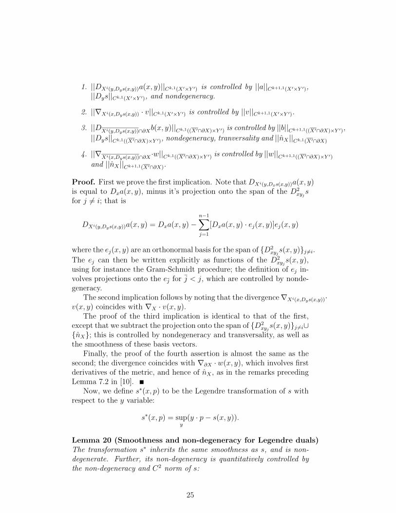
1. ||DXi(y,Dys(x,y))a(x, y)||Ck,1(X′×Y ′) is controlled by ||a||Ck+1,1(X′×Y ′),||Dys||Ck,1(X′×Y ′), and nondegeneracy.

2. ||∇Xi(x,Dys(x,y)) · v||Ck,1(X′×Y ′) is controlled by ||v||Ck+1,1(X′×Y ′).

3. ||DXi(y,Dys(x,y))∩∂Xb(x, y)||Ck,1((X′∩∂X)×Y ′) is controlled by ||b||Ck+1,1((X′∩∂X)×Y ′),

||Dys||Ck,1((X′∩∂X)×Y ′), nondegeneracy, tranversality and ||nX ||Ck,1(X′∩∂X)

4. ||∇Xi(x,Dys(x,y))∩∂X ·w||Ck,1((X′∩∂X)×Y ′) is controlled by ||w||Ck+1,1((X′∩∂X)×Y ′)and ||nX ||Ck+1,1(X′∩∂X).

Proof. First we prove the first implication. Note thatDXi(y,Dxs(x,y))a(x, y)is equal to Dxa(x, y), minus it’s projection onto the span of the D2

xyjs

for j 6= i; that is

DXi(y,Dys(x,y))a(x, y) = Dxa(x, y)−n−1∑j=1

[Dxa(x, y) · ej(x, y)]ej(x, y)

where the ej(x, y) are an orthonormal basis for the span of {D2xyjs(x, y)}j 6=i.

The ej can then be written explicitly as functions of the D2xyjs(x, y),

using for instance the Gram-Schmidt procedure; the definition of ej in-volves projections onto the ej for j < j, which are controlled by nonde-generacy.

The second implication follows by noting that the divergence∇Xi(x,Dys(x,y))·v(x, y) coincides with ∇X · v(x, y).

The proof of the third implication is identical to that of the first,except that we subtract the projection onto the span of {D2

xyjs(x, y)}j 6=i∪

{nX}; this is controlled by nondegeneracy and transversality, as well asthe smoothness of these basis vectors.

Finally, the proof of the fourth assertion is almost the same as thesecond; the divergence coincides with ∇∂X ·w(x, y), which involves firstderivatives of the metric, and hence of nX , as in the remarks precedingLemma 7.2 in [10].

Now, we define s∗(x, p) to be the Legendre transformation of s withrespect to the y variable:

s∗(x, p) = supy

(y · p− s(x, y)).

Lemma 20 (Smoothness and non-degeneracy for Legendre duals)The transformation s∗ inherits the same smoothness as s, and is non-degenerate. Further, its non-degeneracy is quantitatively controlled bythe non-degeneracy and C2 norm of s:

25

inf|u|=1|D2

xps∗(x, p) · u| ≥

inf |v|=1 |D2xys(x, y) · v|

||D2yys(x, y)||

for p = Dys(x, y).

Proof. Uniform convexity implies that s∗ is continuously twice differen-tiable with respect to p. The implicit function theorem combined withthe identity Dps

∗(x,Dys(x, y)) = y implies the smoothness of s∗. Inparticular, differentiating with respect to x yields

D2xps∗(x,Dys(x, y)) = −D2

xys(x, y)D2pps∗(x,Dys(x, y))

and so invertibility of D2pps∗ and nondegeneracy of s imply nondegener-

acy of s∗, and we have, for |u| = 1,

D2xps∗(x,Dys(x, y)) · u=−D2

xys(x, y)D2pps∗(x,Dys(x, y)) · u

=−D2xys(x, y)

D2pps∗(x,Dys(x, y)) · u

|D2pps∗(x,Dys(x, y)) · u|

|D2pps∗(x,Dys(x, y)) · u|.

Now note that setting v = D2pps∗(x,Dys(x, y)) · u = [D2

yys(x, y)]−1 · u, sothat 1 = |u| = |D2

yys(x, y) · v| ≤ ||D2yys(x, y)|| · |v|. Therefore

|v| ≥ 1

||D2yys(x, y)||

and the result follows.Now, we can identify the set X1(y, p) = {x | Dps

∗(x, p) = y}. Wethen define X∗i≤ (y, p), X∗i(y, p) and Φ∗i analogously to above, and com-pute

∂Φ∗i

∂yi=

∫X∗i= (y,p)

f(x, y)

|DX∗is∗pi |dHm−n−1(x) +

∫X∗i≤ (y,p)

∂f

∂yi(x, y)dHm−n(x)

(54)for a.e. (y, p) as long as f and fyi are Lipschitz.

Analogs of Lemmas 17, 18 and 19 when s(x, y) is replaced by s∗(x, p)then follow immediately. We note that

DXi∗s∗pi(x, y) := DXi∗ (y,p)s∗pi

(x, p)∣∣∣p=Dys(x,y)

is defined throughout X ′ × Y ′. We define n∗i, V ∗i, n∗i∂ , n∗iX , V ∗i analo-gously to their un-starred counterparts and note that upon evaluating atp = Dys(x, y), each can be considered a function on X ′×Y ′ or ∂X ′×Y ′.

26

Lemma 21 (Flux derivatives through moving surfaces) Use a :X ′ × Y ′ × P ′ → R Lipschitz to define Φ(y, p) :=

∫X1(y,p)

a(x, y, p)dHm−n(x)

and Ψ(y, p) :=∫X1(y,p)∩∂X a(x, y, p)dHm−n−1(x). Then Φ and Ψ are Lip-

schitz with partial derivatives given almost everywhere by:

∂Φ(y, p)

∂pi=

∫X1(y,p)

[∇Xi(y,p) ·

(a(x, y, p)

DXisyi|DXisyi |

)V i · ni

]p=Dys(x,y)

dHm−n(x)

−∫(

X1(y,p)

)∩∂X

[(a(x, y, p)

DXisyi|DXisyi |

)· niXV i

∂ · ni∂]p=Dys(x,y)

dHm−n−1(x)

+

∫X1(y,p)

[∂a(x, y, p)

∂pi

]p=Dys(x,y)

dHm−n(x), (55)

∂Ψ(y, p)

∂pi=∫X1(y,p)∩∂X

[∇Xi(y,p)∩∂X ·

(a(x, y, p)

DXi(y,p)∩∂Xsyi

|DXi(y,p)∩∂Xsyi |

)V i∂ · ni∂

]p=Dys(x,y)

dHm−n(x)

+

∫X1(y,p)∩∂X

[∂a(x, y, p)

∂pi

]p=Dys(x,y)

dHm−n−1(x), (56)

∂Φ(y, p)

∂yi=

∫X1(y,p)

[∇X∗i(y,p) ·

(a(x, y, p)

DX∗is∗pi

|DX∗is∗pi |

)V ∗i · n∗i

]p=Dys(x,y)

dHm−n(x)

−∫(

X1(y,p)

)∩∂X

[(a(x, y, p)

DX∗is∗pi

|DX∗ispi |

)· n∗iXV ∗i∂ · n∗i∂

]p=Dys(x,y)

dHm−n−1(x)

+

∫X1(y,p)

[∂a(x, y, p)

∂yi

]p=Dys(x,y)

dHm−n(x), (57)

and

∂Ψ(y, p)

∂yi=∫X1(y,p)∩∂X

[∇X∗i(y,p)∩∂X ·

(a(x, y, p)

DX∗i(y,p)∩∂Xs∗pi

|DX∗i(y,p)∩∂Xs∗pi|

)V ∗i∂ · n∗i∂

]p=Dys(x,y)

dHm−n(x)

+

∫X1(y,p)∩∂X

[∂a(x, y, p)

∂yi

]p=Dys(x,y)

dHm−n−1(x). (58)

Proof. We begin by establishing the formulas assuming a ∈ C1,1(X ′ × Y ′ × P ′).

27

Using the generalized divergence theorem [24, Proposition 5.8] wehave, for fixed pi < pi, denoting by p(i) the vector whose i-th entry is pi

and all other entries are equal to those of p,

Φ(y, p) =

∫X1(y,p)

(a(x, y, p)

DXisyi|DXisyi |

)· nidHm−n(x)

=

∫Xi≤(y,p)\Xi

≤(y,p(i))

∇Xi(y,p) ·(a(x, y, p)

DXisyi|DXisyi |

)dHm−n+1(x)

+

∫Xi

=(y,p(i))

(a(x, y, p)

DXisyi|DXisyi|

)· ni(x, y)dHm−n(x)

−∫(

Xi≤(y,p)\Xi

≤(y,p(i))

)∩∂X

(a(x, y, p)

DXisyi|DXisyi |

)· niX(x, y)dHm−n(x).

Noting that the integrands in the first and third terms above are bounded,one can then combine the chain rule with (52) and (53) to differentiatewith respect to pi, getting

∂Φ(y, p)

∂pi=

∫Xi

=(y,p)

∇Xi(y,p) ·(a(x, y, p)

DXisyi|DXisyi |

)V i · nidHm−n(x)

−∫(

Xi=(y,p)

)∩∂X

(a(x, y, p)

DXisyi|DXisyi|

)· niXV i

∂ · ni∂dHm−n−1(x)

+

∫X1(y,p)

∂a(x, y, p)

∂pidHm−n(x).

Finally, notice that one may substitute p = Dys(x, y) in each integrand,

as each region of integration is contained in X1(y, p), to establish (55)for a ∈ C1,1.

Now, note that the formula (55) for ∂Φ(y,p)∂pi

is controlled by ||a||C0,1

(that is, it does not depend on ||a||C1,1). For a merely Lipschitz, we cantherefore choose a sequence an ∈ C1,1 converging to a in the C0,1 norm;passing to the limit implies that ||Φ||C0,1(Y ′×P ′) is controlled by ||a||C0,1 ,and, using the dominated convergence theorem, one obtains the desiredformula.

A similar argument applies to the boundary integral terms to producethe desired formula (56) for ∂Ψ(y,p)

∂pi, while essentially identical arguments

apply to the y derivatives, yielding (57) and (58).

Corollary 22 (Iterated derivative bounds) The operators

Api : (a, b) 7→ (aip, bip) and Ayi : (a, b) 7→ (aiy, b

iy),

28

given by

aip :=[∇Xi(y,p) ·

(a(x, y)

DXisyi|DXisyi |

)V i · ni

]p=Dys(x,y)

,

bip :=[(a(x, y)

DXisyi|DXisyi |

)· niXV i

∂ · ni∂

+∇Xi(y,p)∩∂X ·(b(x, y)

DXi(y,p)∩∂Xsyi

|DXi(y,p)∩∂Xsyi |

)V i∂ · ni∂

]p=Dys(x,y)

,

aiy :=[∇X∗i(y,p) ·

(a(x, y)

DX∗is∗pi

|DX∗is∗pi |

)V ∗i · n∗i +

∂a(x, y)

∂yi

]p=Dys(x,y)

, and

biy :=[∂b(x, y)

∂yi+(a(x, y)

DX∗is∗pi

|DX∗is∗pi|

)· n∗iXV ∗i∂ · n∗i∂

+∇X∗i(y,p)∩∂X ·(b(x, y)

DX∗i(y,p)∩∂Xs∗pi

|DX∗i(y,p)∩∂Xs∗pi|

)V ∗i∂ · n∗i∂

]p=Dys(x,y)

,

define mappings Api : Bk → Bk−1 and Ayi : Bk → Bk−1 between Banachspaces defined by

Bk := Ck,1(X ′ × Y ′)⊕ Ck,1([X ′ ∩ ∂X]× Y ′)

with norms

||Api || ≤ ||1

|DXisyi |||Ck−1,1(X′×Y ′)||ni||Ck−1,1(X′×Y ′)

+ ||ni||Ck−1,1(X′×Y ′)||niX ||Ck−1,1((X′∩∂X)×Y ′)||Vi∂ · ni∂||Ck−1,1((X′∩∂X)×Y ′)

+ ||DXi(y,p)∩∂Xsyi

|DXi(y,p)∩∂Xsyi |||Ck−1,1((X′∩∂X)×Y ′)||V

i∂ ||Ck−1,1((X′∩∂X)×Y ′)||n

i∂||Ck−1,1((X′∩∂X)×Y ′)

and

||Ayi || ≤ ||1

|DX∗is∗pi |||Ck−1,1(X′×Y ′)||n∗i||Ck−1,1(X′×Y ′) + 1

+||n∗i||Ck−1,1(X′×Y ′)||n∗iX ||Ck−1,1((X′∩∂X)×Y ′)||V∗i∂ · n∗i∂ ||Ck−1,1((X′∩∂X)×Y ′)

+||DX∗i(y,p)∩∂Xs

∗pi

|DX∗i(y,p)∩∂Xs∗pi|||Ck−1,1((X′∩∂X)×Y ′)||V

∗i∂ ||Ck−1,1((X′∩∂X)×Y ′)||n

∗i∂ ||Ck−1,1((X′∩∂X)′×Y ′)

controlled by ||Dys||Ck,1, ||nX ||Ck,1, non-degeneracy and transversality.Furthermore, restricted to the subspace Ck,1(X ′×Y ′)⊕{0}, the norms

||Api ||Ck,1(X′×Y ′)⊕{0}→Bk−1≤ || 1

|DXisyi|||Ck−1,1(X′×Y ′)||ni||Ck−1,1(X′×Y ′)

+ ||ni||Ck−1,1(X′×Y ′)||niX ||Ck−1,1((X′∩∂X)×Y ′)||Vi∂ · ni∂||Ck−1,1((X′∩∂X)×Y ′)

29

and

||Ayi ||Ck,1(X′×Y ′)⊕{0}→Bk−1≤ || 1

|DX∗is∗pi|||Ck−1,1(X′×Y ′)||n∗i||Ck−1,1(X′×Y ′) + 1

+ ||n∗i||Ck−1,1(X′×Y ′)||n∗iX ||Ck−1,1((X′∩∂X)×Y ′)||V∗i∂ · n∗i∂ ||Ck−1,1((X′∩∂X)×Y ′)

are controlled by ||Dys||Ck,1, ||nX ||Ck−1,1, non-degeneracy and transver-sality.

Proof. The estimates on the norms follow by simple calculations. Thecontrol on the various quantities in the estimates relies on Lemmas 18,19, 20, and closure of the Holder spaces Ck−1,1 under composition.

We now prove the result announced at the beginning of this section:Proof Theorem 14. First note that as Q enters the definition ofof G1 only through the integrand, whose dependence on Q is smooth,computing derivatives with respect to Q is straightforward.

Corollary 22 allows us to iterate derivatives with respect to the othervariables; given multi indices α = (α1, α2, ...αn), β = (β1, β2, ..., βn), and

γ = (γ1, γ2, ...., γn2) with |α|+ |β|+ |γ| =∑n

i=1 αi +∑n

i=1 βi +∑n2

i=1 γi =k ≤ r, then Lemma 21 and Corollary 22 allow us to compute

∂kG1

∂pα∂yβ∂Qγ=

∫X1(y,p)

aα,βdHm−n +

∫∂X1(y,p)∩∂X1

bα,βdHm−n−1 (59)

where (aα,β, bα,β) = AαAβ(∂|γ|h∂Qγ

, 0) ∈ Br−k, with h(x, y,Q) =det[Q−D2

yys(x,y)]√detD2

xys(x,y)(D2xys(x,y))T

f(x)

being the original integrand in the definition of G1(y, p,Q), and Aα =Aα1p1....Aαnpn , Aβ = Aβ1y1 ....A

βnyn . Now, Corollary 22 implies that ||(aα,β, bα,β)||Cr−k,1

is controlled by ||f ||Cr,1 , ||Dys||Cr+1,1 , ||nX ||Cr−1,1 , non-degeneracy andtransversality.

It then follows from (59) that ∂kG1

∂pα∂yβ∂Qγis controlled by the quantities

listed in the statement of the present theorem for k ≤ r, as desired.

7 Smoothness of the local operator G2 for one di-mensional targets

Taken together, the two preceding sections allow one to bootstrap fromC2,α to higher regularity, when X2 = X1. This raises the followingnatural questions:

1. When X2 and X1 differ (in which case the results in the previoussubsection do not tell us much about solutions of the i = 2 equa-tion), under what conditions is the elliptic operator G2 smooth?

30

2. When can we confirm solutions are C2,α, allowing one to applyTheorem 13?

The goal of this section and the next is to fill these gaps for onedimensional targets, n = 1. In this section, we identify conditions underwhich G2 is smooth. As in the previous section, where regularity of G1

for higher dimensional targets was considered, the general strategy isto adapt the approach in [10], using the divergence theorem to convertintegrals over regions to those over boundaries, and differentiating thelatter using the calculus of moving boundaries. These results, combinedwith general ODE theory, imply that C1,1

loc solutions to the i = 2 equationare in fact C2,1

loc ; higher order regularity estimates on G2 in turn yieldhigher order regularity of these solutions.

The second question above is deferred to Section 8, where we findconditions under which any almost everywhere solution to the i = 2equation with the one dimensional targets is locally C1,1; the resultsof the present section then imply that these solutions are smoother,depending on the degree of regularity of G2.

Given open regions Y ′, P ′ and Q′ in R, throughout this section weset X ′ = ∪(y,p,q)∈Y ′×P ′×Q′X2(y, p, q) and assume:

Assume m ≥ n = 1 in (10)–(11), sy := Dys ∈ C2(X × Y ), (60)

X ⊂ Rm is bounded, ∂X ∈ C1, (61)

D2xys and D3

xyys are linearly independent throughout X ′ × Y ′, (62)

and (65)–(68) below are all finite and positive. (63)

As p is increased, the domain W≤(y, p) := {x ∈ X | sy ≤ p} expandsmonotonically outward with normal velocity w(x, y) := |D2

xys|−1 alongits interface W= = X1. Its normal velocity with respect to changes in yis −syyw. Similarly, as q is increased Z≤(y, q) := {x ∈ X | syy ≤ q} ex-pands monotonically outward with normal velocity z(x, y) := |D3

xyys|−1

along its interface Z=(y, q) := {x ∈ X | syy = q}; its normal veloc-ity with respect to changes in y is −syyyz. Our linear independenceassumption guarantees these velocities are finite and W= intersects Z=

transversally. Notice X2(y, p, q) = W=(y, p)∩Z≤(y, q). Also, in the sameregion of interest, (63) implies that both W= ∩ Z≤ and W≤ ∩ Z= inter-sect ∂X transversally. We denote by nW = wD2

xys and nZ = zD3xyys the

outer normals to W≤ and Z≤ respectively, and observe that the frontierof e.g. W≤ moves with velocity w/ sin θ in Z=, when nZ · nW = cos θ.

Our main result in this section is the following theorem.

Theorem 23 (Smoothness of the ODE given by G2) If n = 1 andr ≥ 0 is an integer then ||G2||Cr,1(Y ′×P ′×Q′) is controlled by ||f ||Cr,1(X′),

31

||sy||Cr+2,1(Y ′×X′), ||nX ||(Cr−1,1∩C0∩W 1,1)(X′∩∂X) and

inf(x,y)∈X′×Y ′

min{|D2xys(x, y)|, |D3

xyys(x, y)|} (non-degeneracy), (64)

inf(x,y)∈(X′∩∂X)×Y ′

1− (nW · nX)2 (p/boundary transversality),(65)

infy∈Y ′, x∈∂X∩W≤(y,P ′)∩Z=(y,Q′)

1− (nZ · nX)2 (q/boundary transversality),(66)

infy∈Y ′, x∈W=(y,P ′)∩Z=(y,Q′)

1− (nW · nZ)2 (p/q transversality), (67)

infy∈Y ′, x∈∂X∩W=(y,P ′)∩Z=(y,Q′)

λ21+λ22+λ23=1

|λ1nW + λ2nZ + λ3nX | (linear independence), (68)

sup(y,p,q)∈Y ′×P ′×Q′

Hm−1(W=(y, p) ∩ Z≤(y, q)) (1st level set size), (69)

sup(y,p,q)∈Y ′×P ′×Q′

Hm−1(W≤(y, p) ∩ Z=(y, q)) (2nd level set size), (70)

sup(y,p,q)∈Y ′×P ′×Q′

Hm(W≤(y, p) ∩ Z≤(y, q)) (iterated sublevel size), (71)

sup(y,p,q)∈Y ′×P ′×Q′

Hm−2((W=(y, p) ∩ Z≤(y, q)) ∩ ∂X) (1st boundary level size), (72)

sup(y,p,q)∈Y ′×P ′×Q′

Hm−2((W≤(y, p) ∩ Z=(y, q)) ∩ ∂X) (2nd boundary level size), (73)

and

sup(y,p,q)∈Y ′×P ′×Q′

Hm−1((W≤(y, p) ∩ Z≤(y, q)) ∩ ∂X) (boundary sublevels size). (74)

We note that, as in [10], since the divergence operator on ∂X involvesfirst derivatives of the metric, which is as smooth as the outward unitnormal ∂X, we require nX ∈ W 1,1 to define ∇∂X ·. By conventionC−1,1 := L∞.

Remark 24 (Convention) We interpret the infimum in the linear in-dependence assumption (68) to be 1 when ∂X ∩W=(y, P ′) ∩ Z=(y,Q′)is empty. When m = 2, this is the only case for which the assumptioncan hold (since three vectors in two dimensions cannot be linearly inde-pendent). When m = 2, positivity of (67) implies W=(y, p)∩Z=(y, q) isdiscrete; with the interpretation above, assumption (68) amounts to thecondition that this set be disjoint from ∂X for all (p, q) ∈ P ′ ×Q′.

Remark 25 (Simplified hypotheses) Note the positivity of (64) fol-lows from (62), while (71) and (74) are controlled byHm[X] andHm−1[∂X].Together with (48) and supy∈Y ′ ‖sy‖C1,1(X), the same quantities control(69) and (70) by Lemma 7.2 of [10]. Finiteness and positivity of theremaining quantities (72)–(73) listed in the theorem follows from thetransversality hypothesized in (63).

32

Example 26 (Annulus to circle revisited) Consider the annulus tocircle example of Example 7, on a domain Y ′ = Y = {θ | θ ∈ (−π, π)}again embedded in R2 by y(θ) = (cos(θ), sin(θ)), with P ′= Q′ = (−ε, ε)small neighbourhoods around the solution v(y) = 0 explicitly computedthere. It remains to verify the transversality hypotheses (63).

It is straightforward to see that W=(y(θ), p) = X1(y(θ), p) = {x | x ·(− sin(θ), cos(θ)) = p} and Z=(y(θ), q) = {x | x · (− cos(θ), sin(θ)) = q}are orthogonal line segments passing near the origin; for ε < 2−1/2 theydo not intersect on the boundary ∂X = {x | 1 = |x|} of X, renderingcondition (68) vacuous. Since the normals to W= and Z= are orthogonalto each other, and do not parallel nX at the points where W= (respectivelyZ=) intersect ∂X, the other three transversality conditions hold as well.

Lemma 27 (Derivatives on moving submanifolds-with-boundary)Given real-valued Lipschitz functions a, b, c on X ′ × Y ′ × P ′ × Q′, anda∂, b∂, c∂ on ∂X ′ × Y ′ × P ′ ×Q′, the functions

A(y, p, q) :=

∫X2(y,p,q)

a(x, y, p, q)dHm−1(x),

B(y, p, q) :=

∫W≤(y,p)∩Z≤(y,q)

b(x, y, p, q)dHm(x),

C(y, p, q) :=

∫W≤(y,p)∩Z=(y,q)

c(x, y, p, q)dHm−1(x),

A∂(y, p, q) :=

∫(W=(y,p)∩Z≤(y,q))∩∂X

a∂(x, y, p, q)dHm−2(x),

B∂(y, p, q) :=

∫(W≤(y,p)∩Z≤(y,q))∩∂X

b∂(x, y, p, q)dHm−1(x) and

C∂(y, p, q) :=

∫(W≤(y,p)∩Z=(y,q))∩∂X

c∂(x, y, p, q)dHm−2(x)

are all Lipschitz, with derivatives given almost everywhere by the formu-lae in Appendix A. Here w := |D2

xys|−1 and z := |D3xyys|−1 as above.

Proof. The proof is similar to the proofs of Lemma 7.4 in [10] andLemma 21 in the present paper; we only described the main differenceshere. For a sufficiently smooth integrand, the derivative of A with re-spect to p, for example, includes a term capturing differentiation of theintegrand with respect to a, and a term capturing the dependence of theregion of integration, which we compute using the generalized divergencetheorem and Lemma 5.1 in [10]:

33

Ap−∫X2

apdHm−1 =∂

∂p

∣∣∣∣p=p

∫W=(y,p)∩Z≤(y,q)

a(x, y, p, q)nW · nWdHm−1(x)

=∂

∂p

[ ∫W≤∩Z≤

∇ · (anW )dHm −∫W≤∩Z=

anW · nZdHm−1 −∫W≤∩Z≤∩∂X

anW · nXdHm−1

]p=p

=

∫W=∩Z≤

∇ · (anW )wdHm−1 −∫W=∩Z=

awnW · nZ√1− (nW · nZ)2

dHm−2

−∫W=∩Z≤∩∂X

awnW · nX√1− (nW · nX)2

dHm−2.

The result for Lipschitz functions can be obtained as in Lemma 7.4 in[10] and Lemma 21 here, via approximation by C1,1 integrands and thedominated convergence theorem. The arguments for other derivativesof A, B and C are similar. We treat boundary integrals analogously.Noting that, for instance,

A∂(y, p, q) =

∫(W=∩Z≤)∩∂X)

a∂(x, y, p, q)dHm−2(x)

=

∫(W≤∩Z≤)∩∂X)

∇∂X · (a∂n∂,W )dHm−1(x)−∫

(W≤∩Z=)∩∂X)

a∂n∂,W · n∂,ZdHm−2(x),

where n∂,W and n∂,Z are defined in Appendix A, we can again use Lemma5.1 in [10] to differentiate with respect to p. Similar arguments apply toall derivatives of A∂, B∂ and C∂.

We note that all integrals over the domain W=∩Z= can be rewrittenusing the divergence theorem as follows:∫

W=∩Z=

a(x, y, p, q)dHm−2(x) =

∫W=∩Z≤

∇W= · (αnW=,Z)dHm−1(x)

−∫

(W=∩Z≤)∩∂XanW=,Z · nW=,XdHm−2(x)

where nW=,Z := nZ−(nZ ·nW )nW√1−(nZ ·nW )2

and nW=,X := nX−(nX ·nW )nW√1−(nX ·nW )2

are the out-

ward unit normals in the submanifold W= ⊆ X to Z≤ and X, respec-tively.

Similarly,

∫(W=∩Z=)∩∂X

a(x, y, p, q)dHm−3(x) =

∫(W=∩Z≤)∩∂X

∇W=∩∂X · (anW=∩∂X,Z)dHm−2(x),

where nW=∩∂X,Z is the outward unit normal to Z≤ ∩ (W= ∩ ∂X) in thecodimension 2 submanifold (W= ∩ ∂X); alternatively, it is equal to nZ ,

34

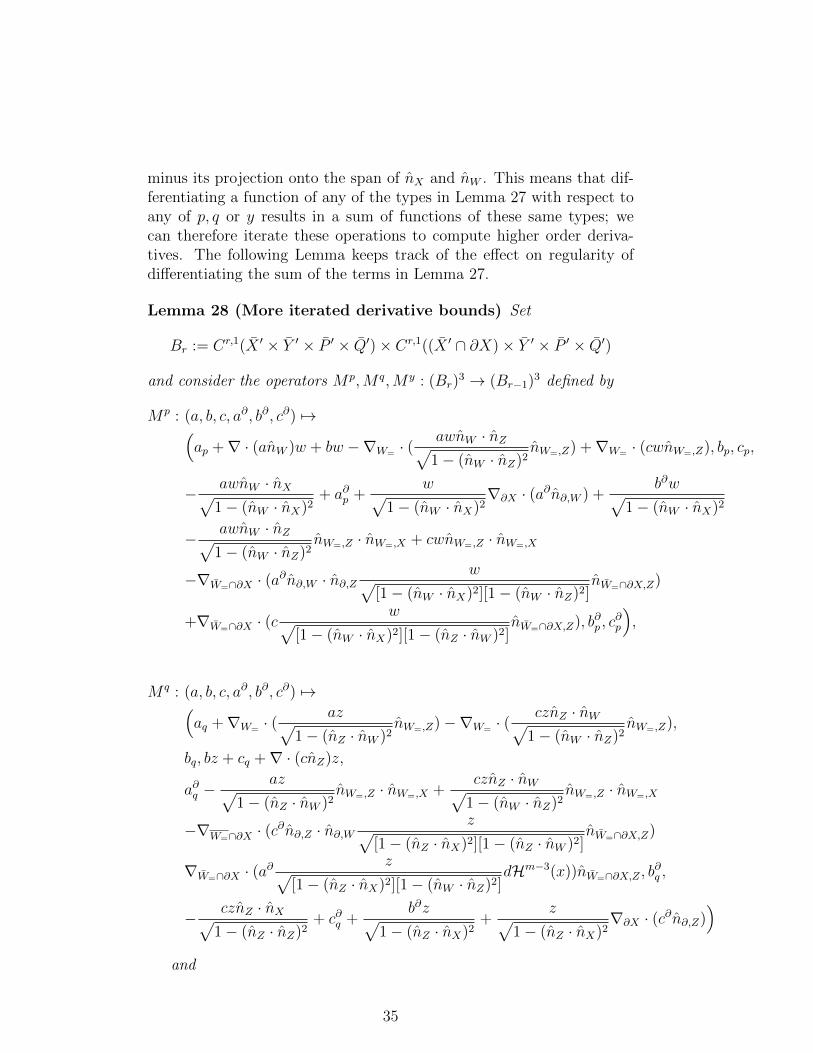
minus its projection onto the span of nX and nW . This means that dif-ferentiating a function of any of the types in Lemma 27 with respect toany of p, q or y results in a sum of functions of these same types; wecan therefore iterate these operations to compute higher order deriva-tives. The following Lemma keeps track of the effect on regularity ofdifferentiating the sum of the terms in Lemma 27.

Lemma 28 (More iterated derivative bounds) Set

Br := Cr,1(X ′ × Y ′ × P ′ × Q′)× Cr,1((X ′ ∩ ∂X)× Y ′ × P ′ × Q′)

and consider the operators Mp,M q,My : (Br)3 → (Br−1)3 defined by

Mp : (a, b, c, a∂, b∂, c∂) 7→(ap +∇ · (anW )w + bw −∇W= · (

awnW · nZ√1− (nW · nZ)2

nW=,Z) +∇W= · (cwnW=,Z), bp, cp,

− awnW · nX√1− (nW · nX)2

+ a∂p +w√

1− (nW · nX)2∇∂X · (a∂n∂,W ) +

b∂w√1− (nW · nX)2

− awnW · nZ√1− (nW · nZ)2

nW=,Z · nW=,X + cwnW=,Z · nW=,X

−∇W=∩∂X · (a∂n∂,W · n∂,Z

w√[1− (nW · nX)2][1− (nW · nZ)2]

nW=∩∂X,Z)

+∇W=∩∂X · (cw√

[1− (nW · nX)2][1− (nZ · nW )2]nW=∩∂X,Z), b∂p , c

∂p

),

M q : (a, b, c, a∂, b∂, c∂) 7→(aq +∇W= · (

az√1− (nZ · nW )2

nW=,Z)−∇W= · (cznZ · nW√

1− (nW · nZ)2nW=,Z),

bq, bz + cq +∇ · (cnZ)z,

a∂q −az√

1− (nZ · nW )2nW=,Z · nW=,X +

cznZ · nW√1− (nW · nZ)2

nW=,Z · nW=,X

−∇W=∩∂X · (c∂n∂,Z · n∂,W

z√[1− (nZ · nX)2][1− (nZ · nW )2]

nW=∩∂X,Z)

∇W=∩∂X · (a∂ z√

[1− (nZ · nX)2][1− (nW · nZ)2]dHm−3(x))nW=∩∂X,Z , b

∂q ,

− cznZ · nX√1− (nZ · nZ)2

+ c∂q +b∂z√

1− (nZ · nX)2+

z√1− (nZ · nX)2

∇∂X · (c∂n∂,Z))

and

35

My : (a, b, c, a∂, b∂, c∂) 7→(ay −∇ · (anW )wsyy − bwsyy − c

∂nZ∂y· nW ,

∇ · (a∂nW∂y

) + by +∇ · (c∂nZ∂y

),

−a∂nW∂y· nZ − bzsyyy + cy −∇ · (cnZ)zsyyy,

awsyynW · nX√1− (nW · nX)2

+ a∂y +wsyy√

1− (nW · nX)2∇∂X · (a∂n∂,W )− b∂wsyy√

1− (nW · nX)2−

c∂∂n∂,Z∂y

· n∂,W ,

−a∂nW∂y· nX − c

∂nZ∂y· nX +∇∂X · (a∂

∂n∂,W∂y

) + b∂y +∇∂X · (c∂∂n∂,Z∂y

),

+czsyyynZ · nX√1− (nZ · nX)2

− a∂ ∂n∂,W∂y

· n∂,Z −b∂zsyyy√

1− (nZ · nX)2+ c∂y

− zsyyy√1− (nZ · nX)2

∇∂X · (c∂n∂,Z))

Then the norms ||Mp||, ||M q|| and ||My|| are controlled by non-degeneracy,transversality, linear independence, ||sy||Cr+2,1 and ||nX ||Cr,1.

Proof. It is straightforward to compute:

||Mp|| ≤ 1 + ||nW ||Cr,1||w||Cr,1 + ||w||Cr−1 + || wnW · nZ√1− (nW · nZ)2

nW=,Z ||Cr,1 + ||wnW=,Z ||Cr,1 + 1 + 1

+|| wnW · nX√1− (nW · nX)2

||Cr−1,1 + 1 + || w√1− (nW · nX)2

||Cr−1,1||n∂,W ||Cr,1

+|| w√1− (nW · nX)2

||Cr−1,1 + || wnW · nZ√1− (nW · nZ)2

nW=,Z · nW=,X + ||wnW=,Z · nW=,X ||Cr−1,1

+||n∂,W · n∂,Zw√

[1− (nW · nX)2][1− (nW · nZ)2]nW=∩∂X,Z ||Cr,1

+|| w√[1− (nW · nX)2][1− (nZ · nW )2]

nW=∩∂X,Z)||Cr,1 + 1 + 1.

Similar estimates hold for M q and My, and it is straightforward to seethat the upper bounds are controlled by the indicated quantities.

We are now ready to prove the Theorem 23, on the regularity of G2.Proof. The proof is similar to the proof of Theorem 14; for indicesα, β, γ with α+β+γ ≤ r, we apply the iterated operators (My)α(Mp)β(M q)γ

36

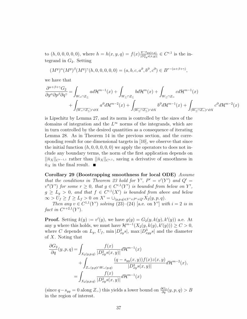
to (h, 0, 0, 0, 0, 0), where h = h(x, y, q) = f(x)q−syy(x,y)|D2xys(x,y)| ∈ C

r,1 is the in-

tegrand in G2. Setting

(My)α(Mp)β(M q)γ(h, 0, 0, 0, 0, 0) = (a, b, c, a∂, b∂, c∂) ∈ Br−(α+β+γ),

we have that

∂α+β+γG2

∂yα∂pβ∂qγ=

∫W=∩Z≤

adHm−1(x) +

∫W≤∩Z≤

bdHm(x) +

∫W≤∩Z=

cdHm−1(x)

+

∫(W=∩Z≤)∩∂X

a∂dHm−2(x) +

∫(W≤∩Z≤)∩∂X

b∂dHm−1(x) +

∫(W≤∩Z=)∩∂X

c∂dHm−2(x)

is Lipschitz by Lemma 27, and its norm is controlled by the sizes of thedomains of integration and the L∞ norms of the integrands, which arein turn controlled by the desired quantities as a consequence of iteratingLemma 28. As in Theorem 14 in the previous section, and the corre-sponding result for one dimensional targets in [10], we observe that sincethe initial function (h, 0, 0, 0, 0, 0) we apply the operators to does not in-clude any boundary terms, the norm of the first application depends on||nX ||Cr−1,1 rather than ||nX ||Cr,1 , saving a derivative of smoothness innX in the final result.

Corollary 29 (Boostrapping smoothness for local ODE) Assumethat the conditions in Theorem 23 hold for Y ′, P ′ = v′(Y ′) and Q′ =v′′(Y ′) for some r ≥ 0, that g ∈ Cr,1(Y ′) is bounded from below on Y ′,g ≥ Lg > 0, and that f ∈ Cr,1(X ′) is bounded from above and below∞ > Uf ≥ f ≥ Lf > 0 on X ′ = ∪(y,p,q)∈Y ′×P ′×Q′X2(y, p, q).

Then any v ∈ C1,1(Y ′) solving (23)–(24) [a.e. on Y ′] with i = 2 is infact in Cr+2,1(Y ′).

Proof. Setting k(y) := v′(y), we have g(y) = G2(y, k(y), k′(y)) a.e. Atany y where this holds, we must have Hm−1(X2(y, k(y), k′(y))) ≥ C > 0,where C depends on Lg, Uf , min |D2

xys|, max |D3xyys| and the diameter

of X. Noting that

∂G2

∂q(y, p, q) =

∫X2(y,p,q)

f(x)

|D2xys(x, y)|

dHm−1(x)

+

∫Z=(y,p)∩W=(y,q)

(q − syy(x, y))f(x)z(x, y)

|D2xys(x, y)|

dHm−2(x),

=

∫X2(y,p,q)

f(x)

|D2xys(x, y)|

dHm−1(x)

(since q−syy = 0 along Z=) this yields a lower bound on ∂G2

∂q(y, p, q) > B

in the region of interest.

37

Therefore, by the Clarke inverse function theorem [11, Theorem7.1.1], q 7→ G2(y, p, q) is invertible; denoting its inverse q(y, p, ·), q isas smooth as G2 (that is, q ∈ Cr,1) and we have, almost everywhere

k′(y) = q(y, k(y), g(y)). (75)

The Lipschitz function k is then equal to the antiderivative of its deriva-tive; for a fixed y0, we have

k(y)− k(y0) =

∫ y

y0

k′(s)ds =

∫ y

y0

q(s, k(s), g(s))ds.

The fundamental theorem of calculus then implies that k is everywheredifferentiable, and that (75) holds for all y. In particular, k′ is Lips-chitz as y 7→ q(y, k(y), g(y)), hence v ∈ C2,1(Y ′). If r > 0, one canimmediately bootstrap to get k′ ∈ Cr,1(Y ′), hence v ∈ Cr+2,1(Y ′).

Remark 30 (Is G2 smooth for higher dimensional targets?) It isnatural to ask whether the proofs of Theorem 14 and 23 can be adaptedto yield smoothness of G2 when n > 1. While this is conceivable, there isa significant hurdle: the structure of the set X2(y, p,Q) is not amenableto our techniques, since it is no longer a manifold-with-boundary; it isat best a manifold-with-corners, and in the absence of additional restric-tions might be worse. To see this, recall X2(y, p,Q) = X1(y, p)∩A(y,Q),where A(y,Q) := {x : Q−D2

yys(x, y) ≥ 0}. Non-negative definitess of ann × n matrix is determined by a system of nonlinear inequalities whosesaturation sets are not generally manifolds — nevermind intersectingtransversally — unless n = 1. These inequalities force the eigenvaluesof Q − D2

yys into the positive orthant. Although the positive orthant isa manifold-with-corners, we know of no implicit function type theoremthat describes the set of x ∈ X1(y, p) satisfying such a system.

8 C1,1 regularity of solutions to the i = 2 ODE

In this section, we’ll assume that n = 1 (one dimensional target), andthat the minimizer (u, v) = (vs, us) to (8) satisfies the local equation(23)–(24) a.e. for i = 2, which also implies (33). Recall v = vss isin C0,1(Y ) and semiconvex from (11). Our goal is to identify a subsetY ′ ⊂ Y on which the initial smoothness hypothesis v ∈ C1,1(Y ′) neededfor the bootstrap (Corollary 29 of the preceding section) is satisfied.

Assume the probability densities f and g satisfy

log f ∈ C(X) and log g ∈ C(Y ), so that (76)

0 < Lf ≤ f(x) ≤ Uf <∞ for all x ∈ X (77)

0 < Lg ≤ g(y) ≤ Ug <∞ for all y ∈ Y. (78)

38

As in Section 7, we’ll assume X, Y and s satisfy (60)–(61). We shallwork on open regions Y ′ ⊂ Y and P ′ ⊂ P = ∂s

∂y(X, Y ) satisfying

inf(y,p)∈Y ′×P ′

Hm−1(X1(y, p)) > 0. (79)

Taking Q′ = R and X ′ = ∪(y,p)∈Y ′×P ′X1(y, p), we’ll assume (46) andpositivity of (48) as in Section 6. In particular, s is uniformly non-degenerate and — without loss of generality — convex with respect toy ∈ Y ′, so that k(y) := v′(y) is non-decreasing, and the upper bound(50) complementing (79) is finite by Remark 25. We shall also requirethe function q(y, p, β) (defined before (75) and recalled in the next para-graph) to be continuous, and that s satisfy an enhanced form of thetwist condition detailed in Assumption 32 below.

The functional

G2(y, p, q) :=

∫X2(y,p,q)

q − syy(x, y)

|D2xys(x, y)|

f(x)dHm−1(x). (80)

is strictly increasing in q on {(y, p, q) | G2 > 0} and diverges as q →∞.For β > 0 and fixed y and p, as in Section 7, denote by q(y, p, β) theunique solution of

q 7→ G2(y, p, q) = β (81)

We therefore have q(y, k(y), g(y)) = k′(y) almost everywhere. Underthe assumptions of Theorem 23 for some r ≥ 0, q(y, p, β) is Lipschitzcontinuous in all its arguments, by the Clarke implicit function theorem,[11, Section 7.1]. Although it holds only almost everywhere, this formu-lation provides some intuition for why we expect k to be Lipschitz, sinceboundedness of k and g imply boundedness of k′ wherever the equationq(y, k(y), g(y)) = k′(y) holds.

The estimate below essentially controls the volume of the regionF−1([y0, y1]) mapped to an interval [y0, y1] by the map F of Theorem2 using the variation in k, compensated by a term reflecting the varia-tion in y. Together with mass balance, this proposition easily impliesthat k is Lipschitz if continuous (and so v ∈ C1,1

loc if v ∈ C1loc), as we will

show in Theorem 35.The continuity of k, assumed in Proposition 31, will be confirmed in

Proposition 34.

Proposition 31 (The derivative of v is Lipschitz if continuous)Let Y ′ ⊂ Y and P ′ ⊂ P = ∂s

∂y(X, Y ) satisfy the hypotheses imposed be-

tween (76) and (80). Then there exist positive constants C1 and C2 suchthat

39

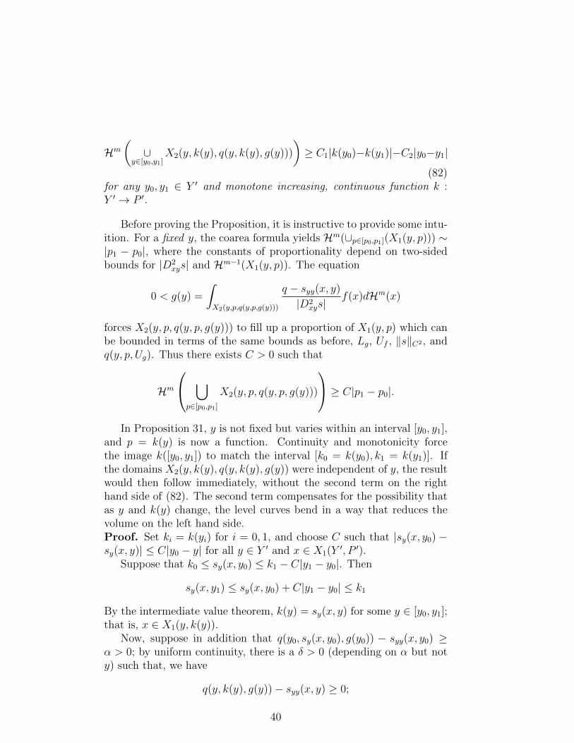
Hm

(∪

y∈[y0,y1]X2(y, k(y), q(y, k(y), g(y)))

)≥ C1|k(y0)−k(y1)|−C2|y0−y1|

(82)for any y0, y1 ∈ Y ′ and monotone increasing, continuous function k :Y ′ → P ′.

Before proving the Proposition, it is instructive to provide some intu-ition. For a fixed y, the coarea formula yields Hm(∪p∈[p0,p1](X1(y, p))) ∼|p1 − p0|, where the constants of proportionality depend on two-sidedbounds for |D2

xys| and Hm−1(X1(y, p)). The equation

0 < g(y) =

∫X2(y,p,q(y,p,g(y)))

q − syy(x, y)

|D2xys|

f(x)dHm(x)

forces X2(y, p, q(y, p, g(y))) to fill up a proportion of X1(y, p) which canbe bounded in terms of the same bounds as before, Lg, Uf , ‖s‖C2 , andq(y, p, Ug). Thus there exists C > 0 such that

Hm

⋃p∈[p0,p1]

X2(y, p, q(y, p, g(y)))

≥ C|p1 − p0|.

In Proposition 31, y is not fixed but varies within an interval [y0, y1],and p = k(y) is now a function. Continuity and monotonicity forcethe image k([y0, y1]) to match the interval [k0 = k(y0), k1 = k(y1)]. Ifthe domains X2(y, k(y), q(y, k(y), g(y)) were independent of y, the resultwould then follow immediately, without the second term on the righthand side of (82). The second term compensates for the possibility thatas y and k(y) change, the level curves bend in a way that reduces thevolume on the left hand side.Proof. Set ki = k(yi) for i = 0, 1, and choose C such that |sy(x, y0) −sy(x, y)| ≤ C|y0 − y| for all y ∈ Y ′ and x ∈ X1(Y ′, P ′).

Suppose that k0 ≤ sy(x, y0) ≤ k1 − C|y1 − y0|. Then

sy(x, y1) ≤ sy(x, y0) + C|y1 − y0| ≤ k1

By the intermediate value theorem, k(y) = sy(x, y) for some y ∈ [y0, y1];that is, x ∈ X1(y, k(y)).

Now, suppose in addition that q(y0, sy(x, y0), g(y0)) − syy(x, y0) ≥α > 0; by uniform continuity, there is a δ > 0 (depending on α but noty) such that, we have

q(y, k(y), g(y))− syy(x, y) ≥ 0;

40

that is, x ∈ X2(y, k(y), q(y, k(y), g(y))), if |y − y0| < δ.Now, note if |y0 − y1| ≥ δ, the right hand side of (82) is negative

for appropriate choices of C1, C2 (note that k(y0) − k(y1) is less thanor equal to the diameter of P ′). We can therefore assume |y0 − y1| <δ without loss of generality, and the above argument then yields x ∈X2(y, k(y), q(y, k(y), g(y))) for some y ∈ [y0, y1].

It therefore follows that

∪p∈[k0,k1−C|y1−y0|]{x ∈ X1(y0, p) | q(y0, p, g(y0))− syy(x, y0) ≥ α}(83)

⊆ ∪y∈[y0,y1]X2(y, k(y), q(y, k(y), g(y)))

Now our definition of q yields g(y0) = G2(y0, p, q(y0, p, g(y0))), whichimplies that for a small enough α, we have

Hm−1({x ∈ X1(y0, k(y)) : q(y0, k(y), g(y0))−syy(x, y0) ≥ α}) ≥ BHm−1(X1(y0, k(y)))

for some B > 0 depending on the lower bound Lg for g, min |D2xys|,

max |D3xyys| and the size of the level sets, sup(y,p)∈Y×k(Y )Hm−1(X1(y, p)).

It then follows that

vol[∪p∈[k0,k1−C|y1−y0|]{x ∈ X1(y0, p) | q(y0, p, g(y0))− syy(x, y0) ≥ α}]≥Bvol[∪p∈[k0,k1−C|y1−y0|]X1(y0, p)] (84)

Now, if k1 − 2C|y1 − y0| ≤ k0, then |k1 − k0| − 2C|y1 − y0| < 0 andthere is nothing to prove, since the right hand side of (82) is negativefor appropriate choices of the constants.

On the other hand, if k1−2C|y1−y0| ≥ k0, then k1−C|y1−y0|−k0 ≥|k1−k0|

2, and so

vol[∪p∈[k0,k1−C|y1−y0|]X1(y0, p)] ≥ D|k1 − k0|

2,

where D depends on the size minp∈[k0,k1]Hm−1(X1(y0, p)) of the levelsets, and the speed limit minsy(x,y0)∈[k0,k1] |D2

xys(y0, x)|. This combinedwith (83) and (84) establishes the result.

Our strategy is to combine Proposition 31 with mass balance to de-duce a Lipschitz condition on k. To apply this Proposition, we must firstshow that k is continuous. We do this under the following strengtheningof the twist condition:

Assumption 32 (Enhanced twist) We say s ∈ C2(X × Y ) satisfiesthe enhanced twist condition if Dxs(x, y)−Dxs(x, y) and D2

xys(x, y) arelinearly independent for each x ∈ X and y, y ∈ Y ⊂ R with y 6= y.

41

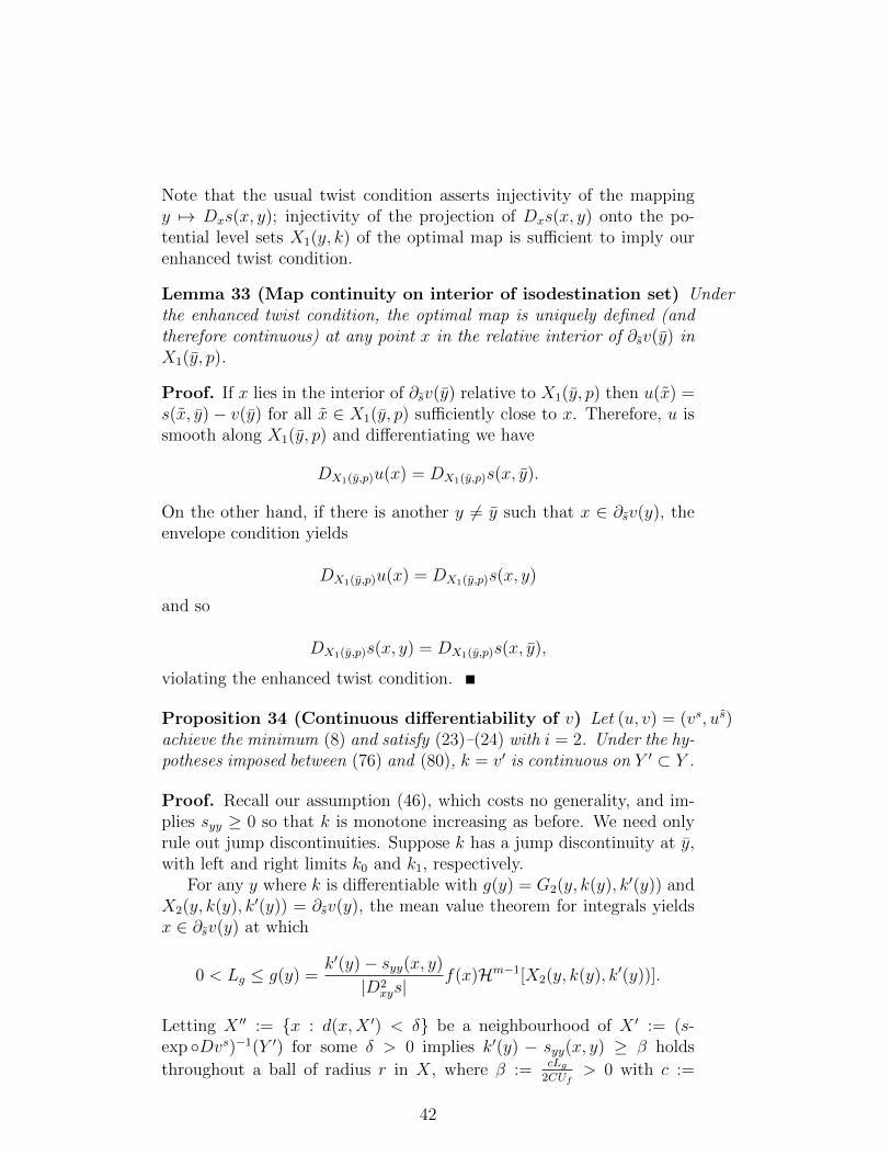
Note that the usual twist condition asserts injectivity of the mappingy 7→ Dxs(x, y); injectivity of the projection of Dxs(x, y) onto the po-tential level sets X1(y, k) of the optimal map is sufficient to imply ourenhanced twist condition.

Lemma 33 (Map continuity on interior of isodestination set) Underthe enhanced twist condition, the optimal map is uniquely defined (andtherefore continuous) at any point x in the relative interior of ∂sv(y) inX1(y, p).

Proof. If x lies in the interior of ∂sv(y) relative to X1(y, p) then u(x) =s(x, y)− v(y) for all x ∈ X1(y, p) sufficiently close to x. Therefore, u issmooth along X1(y, p) and differentiating we have

DX1(y,p)u(x) = DX1(y,p)s(x, y).

On the other hand, if there is another y 6= y such that x ∈ ∂sv(y), theenvelope condition yields

DX1(y,p)u(x) = DX1(y,p)s(x, y)

and so

DX1(y,p)s(x, y) = DX1(y,p)s(x, y),

violating the enhanced twist condition.

Proposition 34 (Continuous differentiability of v) Let (u, v) = (vs, us)achieve the minimum (8) and satisfy (23)–(24) with i = 2. Under the hy-potheses imposed between (76) and (80), k = v′ is continuous on Y ′ ⊂ Y .

Proof. Recall our assumption (46), which costs no generality, and im-plies syy ≥ 0 so that k is monotone increasing as before. We need onlyrule out jump discontinuities. Suppose k has a jump discontinuity at y,with left and right limits k0 and k1, respectively.

For any y where k is differentiable with g(y) = G2(y, k(y), k′(y)) andX2(y, k(y), k′(y)) = ∂sv(y), the mean value theorem for integrals yieldsx ∈ ∂sv(y) at which

0 < Lg ≤ g(y) =k′(y)− syy(x, y)

|D2xys|

f(x)Hm−1[X2(y, k(y), k′(y))].

Letting X ′′ := {x : d(x,X ′) < δ} be a neighbourhood of X ′ := (s-exp ◦Dvs)−1(Y ′) for some δ > 0 implies k′(y) − syy(x, y) ≥ β holds

throughout a ball of radius r in X, where β := cLg2CUf

> 0 with c :=

42

min |D2xys(x, y)|, C := sup(y,k)∈Y×k(Y )Hm−1(X1(y, k)), and r depends

only on δ and B := sup(x,y)∈X”×Y ′ |Dxsyy(x, y)|.Now take a sequence {yi} with yi < y for which this is true, converg-

ing to y. We have that k(yi)→ k0 and, after passing to a subsequence,the centers xi of the corresponding balls converge to an x ∈ X1(y, k0) ∩∂sv(y). By continuity, we have q(y, k0, g(y)) − syy(y, x) ≥ 2β > 0, andtherefore, q(y, k(y), g(y))− syy(y, x) ≥ β > 0 for all (x, y) close to (x, y)with y < y.

Therefore,k′(y)− syy(y, x) ≥ β > 0 (85)

for all x near x, and almost all y < y near y.In addition, since Br(xi) ∩ X1(yi, k(yi)) ⊆ ∂sv(yi), and each x ∈

Br(x) ∩ X1(y, k0) can be approximated by points zi(x) ∈ Br(xi) ∩X1(yi, k(yi)), we can pass to the limit in the equality u(zi(x)) + v(yi) =s(zi(x), yi) to obtain u(x)+v(y) = s(x, y); that is, x ∈ ∂sv(y). Therefore,Br(x) ∩X1(y, k0) ⊂ ∂sv(y).

We have now shown that x is in the relative interior of ∂sv(y) inX1(y, k0). Lemma 33 therefore implies that the optimal map F is con-tinuous at x. We next show that all points in the open set X>(y, k0) :={x ∈ X | sy(x, y) > k0} sufficiently near x must get mapped to y; thisviolates mass balance and establishes the result.

Choose x with sy(x, y) > k0 such that |x− x| < ε, and set y = F (x).The continuity of F at x ensures y is close to y; for ε > 0 sufficiently smallwe shall prove it must actually be equal to y. First observe sy(x, y) < k1

for ε > 0 sufficiently small, since sy(x, y) = k0 < k1.If y > y, then k(y) > k1. In this case, sy(x, y) = k(y) > k1, immedi-

ately yielding a contradiction.On the other hand, if y < y, then (85) implies that

k0 − sy(x, y)− [k(y)− sy(x, y)]≥∫ y

y

[k′(s)− syy(x, s)]ds

≥ β|y − y|

As k0 = sy(x, y), this means, for almost every y < y, with y close toy

sy(x, y)− sy(x, y) = sy(x, y)− k(y) ≥ β|y − y|.Therefore,

sy(x, y)− sy(x, y) = sy(x, y)− sy(x, y) +

∫ y

y

[syy(x, t)− syy(x, t)]dt

≥ β|y − y| −B|y − y||x− x|= |y − y|(β −B|x− x|) > 0.

43

for |x − x| sufficiently small. This contradicts the assumption x ∈X>(y, k0).

To summarize, we have shown that for x ∈ X>(y, k0) close to x, wecannot have F (x) > y or F (x) < y; we must therefore have F (x) = y.As this set has positive mass, and ν({y}) = 0, this violates mass balance,establishing that k cannot have a jump discontinuity.

Theorem 35 (Lipschitz differentiability of v) Let (u, v) = (vs, us)achieve the minimum (8) and solve (23)–(24) a.e. on Y with i = 2. IfY ′ ⊂ Y and P ′ = v′(Y ′) are regions satisfying the hypotheses imposedbetween (76) and (80), then v ∈ C1,1(Y ′).

Proof. Setting k = v′ yields k′(y) = v′′(y) = q(y, k(y), g(y)) almosteverywhere. Choose y0 < y1 and denote k(yi) = ki for i = 1, 2. Since∂sv(y) = X2(y, k(y), k′(y)) = X2(y, k(y), q(y, k(y), g(y))) for a.e. y, massbalance and Propositions 31 and 34 combine to imply

Ug|y1 − y0| ≥∫ y1

y0

g(y)dy (86)

=

∫∪y∈[y0,y1]X2(y,k(y),q(y,k(y),g(y)))

f(x)dHm(x) (87)

≥Lfvol[∪y∈[y0,y1]X2(y, k(y), q(y, k(y), g(y)))] (88)

≥Lf (C1|k(y0)− k(y1)| − C2|y0 − y1|). (89)

This is the desired conclusion.

Remark 36 (Conclusion and comparison to previous work) Combinedwith Corollary 29 of Section 7, Theorem 35 identifies sets Y ′ on whichany solution v = vss to the local equation (23) for i = 2 must be C2,1, orin fact smoother, depending on G2. The main advance in these sectionsover the theory developed in [10] is that solutions are assumed only tosatisfy the weaker i = 2 version of the local equation (23), rather that thestronger i = 1 version implied by the nestedness condition assumed in[10]. This is illustrated by the examples below. On the other hand, ad-ditional assumptions on s are needed here, including the enhanced twistcondition, the third-order linear independence relation (62), and variousconditions involving the geometry of the level sets of x 7→ D2

yys(x, y)and their intersection with level sets of Dys(x, y) implied by the fact that(66)–(68) are assumed positive.

Example 37 (Revisiting the annulus to circle match again) RecallingExample 7, note that

Dxs(x, θ) = y(θ) := (cos θ, sin θ) and

D2xθs(x, θ) = y(θ)⊥ := (− sin θ, cos θ)

44

are perpendicular unit vectors. For distinct θ, θ ∈ Y the linear inde-pendence required by the enhanced twist (Assumption 32) asserts y(θ)−y(θ) 6= ay(θ)⊥ for any scalar a ∈ R. Taking inner products with y(θ)yields y(θ) · y(θ) 6= 1 which is satisfied unless θ = θ mod 2π, or equiv-alently, unless θ = θ since both lie in Y := (−π, π). Thus this sur-plus obeys the enhanced twist condition. The rest of the conditions areeasy to check, so that solutions v = vss to the i = 2 equation with‖v‖C0,1(Y ) < 1 belong to C1,1(Y ) by Theorem 35, and are in fact smootherunder appropriate conditions by Remark 36. From Example 26, the re-quired conditions include a smallness restriction ‖v‖C1,1(Y ) < 2−1/2; when‖v‖C0,1(Y ) << 1 is small, this follows directly from v′′(θ) = q(θ, v′(θ), g(θ))and the hypothesized continuity of q around q(y, 0, 1/2π) = 0.

This applies, for instance, to the problem where the marginals areuniform, solved explicitly by v = 0 in Example 7. More generally, whena uniformly small enough perturbation of the density g(θ) = 1/2π yieldsan a.e. solution v = vss to the i = 2 equation, as in the next example,the above analysis can be applied to deduce smoothness of v. Note thatneither example is nested, so the regularity theory developed in [10] doesnot apply.

Example 38 (Mapping the disk to a weighted interval) Let s(x, θ) =x · (cos(θ), sin(θ)) on X = B(1, 0) ⊆ R2 and Y = (−π, π). Let f be uni-form and choose λ ∈ (−1, 1). Then v(θ) = λ cos(θ) is s-convex andtherefore solves the i = 2 (but not i = 1) equation when g(θ) is definedby

g(θ) = G2(θ, v′(θ), v′′(θ)).

Here X1(θ, v′(θ)) coincides with the line segment through (λ, 0) makingangle θ with the horizontal axis, while X2(θ, v′(θ), v′′(θ)) = ∂sv(θ) is theintersection of this line segment with {θx2 ≥ 0}. As in the preceding ex-ample, the conditions in Theorems 23 and 35 are easily verified, implyingsmoothness of v (in agreement with the explicit solution).

45

Appendices

Appendix A Formulas for partial derivatives

The partial derivatives of the functions defined in Lemma 27 are givenalmost everywhere by the following formulas, with w(x, y) = |D2

xys|−1:

Ap−∫X2

apdHm−1 =∂

∂p

∣∣∣∣p=p

∫W=(y,p)∩Z≤(y,q)

a(x, y, p, q)nW · nWdHm−1(x)

=∂

∂p

[ ∫W≤∩Z≤

∇ · (anW )dHm −∫W≤∩Z=

anW · nZdHm−1 −∫W≤∩Z≤∩∂X

anW · nXdHm−1

]p=p

=

∫W=∩Z≤

∇ · (anW )wdHm−1 −∫W=∩Z=

awnW · nZ√1− (nW · nZ)2

dHm−2

−∫W=∩Z≤∩∂X

awnW · nX√1− (nW · nX)2

dHm−2,

Aq−∫X2

aqdHm−1 =∂

∂q

∣∣∣∣q=q

∫W=(y,p)∩Z≤(y,q)

a(x, y, p, q)dHm−1(x)

=

∫W=∩Z=

az√1− (nZ · nW )2

dHm−2,

Ay−∫X2

aydHm−1 +

∫W=∩Z=

azsyyy√1− (nZ · nW )2

dHm−2 =∂

∂y

∣∣∣∣y=y

∫W=(y,p)∩Z≤(y,q)

a(x, y, p, q)dHm−1(x)

=∂

∂y

[ ∫W≤∩Z≤

∇ · (anW )dHm −∫W≤∩Z=

anW · nZdHm−1 −

∫W≤∩Z≤∩∂X

anW · nXdHm−1

]y=y

=

∫W≤∩Z≤

∇ · (a∂nW∂y

)dHm −∫W≤∩Z=

a∂nW∂y· nZdHm−1 −

∫W≤∩Z≤∩∂X

a∂nW∂y· nXdHm−1

−∫W=∩Z≤

∇ · (anW )wsyydHm−1 +

∫W=∩Z=

awsyynW · nZ√1− (nW · nZ)2

dHm−2

+

∫W=∩Z≤∩∂X

awsyynW · nX√1− (nW · nX)2

dHm−2

where ∂∂ynW = (nZ − nW (nW · nZ))w/z,

Bp =

∫W≤(y,p)∩Z≤(y,q)

bpdHm(x) +

∫W=(y,p)∩Z≤(y,q)

bwdHm−1(x),

Bq =

∫W≤(y,p)∩Z≤(y,q)

bqdHm(x) +

∫W≤(y,p)∩Z=(y,q)

bzdHm−1(x),

46

By =

∫W≤(y,p)∩Z≤(y,q)

bydHm(x)−∫W=(y,p)∩Z≤(y,q)

bwsyydHm−1(x)−∫W≤(y,p)∩Z=(y,q)

bzsyyydHm(x),

Cp =

∫W≤(y,p)∩Z=(y,q)

cpdHm−1(x) +

∫W=(y,p)∩Z=(y,q)

cwdHm−2(x),

Cq =

∫W≤(y,p)∩Z=(y,q)

cqdHm−1(x) +

∫W≤(y,p)∩Z=(y,q)

∇ · (cnZ)zdHm−1(x)

−∫W=(y,p)∩Z=(y,q)

cznZ · nW√1− (n∂,W · n∂,Z)2

dHm−2(x)−∫W≤∩Z=∩∂X

cznZ · nX√1− (nZ · nX)2

dHm−2,

Cy =

∫W≤∩Z=

cydHm−1 −∫W=∩Z=

cwsyy√1− (nZ · nW )2

dHm−2

+

∫W≤∩Z≤

∇ · (c∂nZ∂y

)dHm −∫W=∩Z≤

c∂nZ∂y· nWdHm−1 −

∫W≤∩Z≤∩∂X

c∂nZ∂y· nXdHm−1

−∫W≤∩Z=

∇ · (cnZ)zsyyydHm−1 +

∫W=∩Z=

czsyyynW · nZ√1− (nW · nZ)2

dHm−2

+

∫W≤∩Z=∩∂X

czsyyynZ · nX√1− (nZ · nX)2

dHm−2,

A∂p =

∫(W=∩Z≤)∩∂X)

a∂pdHm−2(x) +

∫(W=∩Z≤)∩∂X)

w√1− (nW · nX)2

∇∂X · (a∂n∂,W )dHm−2(x)

−∫

(W=∩Z=)∩∂X)

a∂n∂,W · n∂,Zw√

[1− (nW · nX)2][1− (n∂,W · n∂,Z)2]dHm−3(x),

A∂q =

∫(W=∩Z≤)∩∂X)

a∂qdHm−2(x) +

∫(W=∩Z=)∩∂X)

a∂z√

[1− (nZ · nX)2][1− (n∂,W · n∂,Z)2]dHm−3(x),

A∂y =

∫(W=∩Z≤)∩∂X)

a∂ydHm−2(x)−∫

(W=∩Z=)∩∂X)

a∂zsyyy√

[1− (nZ · nX)2][1− (n∂,W · n∂,Z)2]dHm−3(x)

+

∫(W≤∩Z≤)∩∂X)

∇∂X · (a∂∂n∂,W∂y

)dHm−1(x)−∫

(W≤∩Z=∩∂X)

a∂∂n∂,W∂y

· n∂,ZdHm−2(x)

+

∫(W=∩Z≤)∩∂X)

wsyy√1− (nW · nX)2

∇∂X · (a∂n∂,W )dHm−2(x)

−∫

(W=∩Z=)∩∂X)

wsyy√[1− (nW · nX)2][1− (n∂,W · n∂,Z)2]

a∂n∂,W · n∂,ZdHm−3(x),

47

where n∂,W := nW−(nW ·nX)nX√1−(nW ·nX)2

and n∂,Z := nZ−(nZ ·nX)nX√1−(nZ ·nX)2

are the outward

unit normals to W≤ ∩ ∂X and Z≤ ∩ ∂X in ∂X, respectively and

B∂p =

∫(W≤∩Z≤)∩∂X)

b∂pdHm−1(x)+

∫(W=∩Z≤)∩∂X)

b∂w√1− (nW · nX)2

dHm−2(x),

B∂q =

∫(W≤∩Z≤)∩∂X)

b∂qdHm−1(x)+

∫(W≤∩Z=)∩∂X)

b∂z√1− (nZ · nX)2

dHm−2(x),

B∂y =

∫(W≤∩Z≤)∩∂X)

b∂ydHm−1(x)−∫

(W=∩Z≤)∩∂X)

b∂wsyy√1− (nW · nX)2

dHm−2(x)

−∫

(W≤∩Z=)∩∂X)

b∂zsyyy√1− (nZ · nX)2

dHm−2(x),

C∂p =

∫(W≤∩Z=)∩∂X)

c∂pdHm−2(x) +

∫(W=∩Z=)∩∂X)

c∂w√

[1− (nW · nX)2][1− (n∂,Z · n∂,W )2]dHm−3(x),

C∂q =

∫(W≤∩Z=)∩∂X)

c∂qdHm−2(x) +

∫(W≤∩Z=)∩∂X)

z√1− (nZ · nX)2

∇∂X · (c∂n∂,Z)dHm−2(x)

−∫

(W=∩Z=)∩∂X)

c∂n∂,Z · n∂,Wz√

[1− (nZ · nX)2][1− (n∂,Z · n∂,W )2]dHm−3(x),

and

C∂y =

∫(W≤∩Z=)∩∂X)

c∂ydHm−2(x)−∫

(W=∩Z=)∩∂X)

c∂wsyy√

[1− (nW · nX)2][1− (n∂,W · n∂,Z)2]dHm−3(x)

+

∫(W≤∩Z≤)∩∂X)

∇∂X · (c∂∂n∂,Z∂y

)dHm−1(x)−∫

(W=∩Z≤∩∂X)

c∂∂n∂,Z∂y

· n∂,WdHm−2(x)

−∫

(W≤∩Z=)∩∂X)

zsyyy√1− (nZ · nX)2

∇∂X · (c∂n∂,Z)dHm−1(x)

+

∫(W=∩Z=)∩∂X)

zsyyy√[1− (nZ · nX)2][1− (n∂,W · n∂,Z)2]

c∂n∂,W · n∂,ZdHm−3(x).

48

References

[1] Luigi Ambrosio and Gianni Dal Maso. A general chain rule fordistributional derivatives. Proc. Amer. Math. Soc., 108:691–702,1990.

[2] Y. Brenier. Decomposition polaire et rearrangement monotone deschamps de vecteurs. C.R. Acad. Sci. Paris Ser. I Math., 305:805–808, 1987.

[3] Y. Brenier. Polar factorization and monotone rearrangement ofvector-valued functions. Comm. Pure Appl. Math., 44:375–417,1991.

[4] H. Brezis. Remarks on the Monge-Kantorovich problem in the dis-crete setting. C. R. Math. Acad. Sci. Paris, 356:207–213, 2018.

[5] L. Caffarelli. Allocation maps with general cost functions. InP. Marcellini et al, editor, Partial Differential Equations and Ap-plications, number 177 in Lecture Notes in Pure and Appl. Math.,pages 29–35. Dekker, New York, 1996.

[6] L.A. Caffarelli. The regularity of mappings with a convex potential.J. Amer. Math. Soc., 5:99–104, 1992.

[7] L.A. Caffarelli. Boundary regularity of maps with convex potentials— II. Ann. of Math. (2), 144:453–496, 1996.

[8] Pierre-Andre Chiappori, Robert McCann, and Brendan Pass. Tran-sition to nestedness in multi- to one-dimensional optimal transport.European J. Appl. Math., 30(6):1220–1228, 2019.

[9] P.-A. Chiappori, R.J. McCann, and B. Pass. Multidimensionalmatching. Preprint.

[10] P.-A. Chiappori, R.J. McCann, and B. Pass. Multi- to one-dimensional optimal transport. Comm. Pure Appl. Math., 70:2405–2444, 2017.

[11] F.H. Clarke. Optimization and nonsmooth analysis. Wiley, NewYork, 1983.

[12] Michael G. Crandall, Hitoshi Ishii, and Pierre-Louis Lions. User’sguide to viscosity solutions of second order partial differential equa-tions. Bull. Amer. Math. Soc. (N.S.), 27(1):1–67, 1992.

[13] M.J.P Cullen and R.J. Purser. An extended Lagrangian model ofsemi-geostrophic frontogenesis. J. Atmos. Sci., 41:1477–1497, 1984.

[14] G. De Philippis and A. Figalli. The Monge-Ampere equation andits link to optimal transportation. Bull. Amer. Math. Soc. (N.S.),51(4):527–580, 2014.

[15] G. De Philippis and A. Figalli. Partial regularity for optimal trans-port maps. Publ. Math. Inst. Hautes Etudes Sci., 121:81–112, 2015.

[16] P. Delanoe. Classical solvability in dimension two of the secondboundary-value problem associated with the Monge-Ampere oper-

49

ator. Ann. Inst. H. Poincare Anal. Non Lineaire, 8:443–457, 1991.[17] L.C. Evans and R.F. Gariepy. Measure Theory and Fine Properties

of Functions. Stud. Adv. Math. CRC Press, Boca Raton, 1992.[18] A. Figalli. Regularity properties of optimal maps between noncon-

vex domains in the plane. Comm. Partial Differential Equations,35:465–479, 2010.

[19] A. Figalli and N. Gigli. Local semiconvexity of Kantorovich po-tentials on non-compact manifolds. ESAIM Control Optim. Calc.Var., 17:648–653, 2011.

[20] A. Figalli and Y.-H. Kim. Partial regularity of Brenier solutions ofthe Monge-Ampere equation. Discrete Contin. Dyn. Syst., 28:559–565, 2010.

[21] W. Gangbo and R.J. McCann. The geometry of optimal transporta-tion. Acta Math., 177:113–161, 1996.

[22] W. Gangbo and R.J. McCann. Shape recognition via Wassersteindistance. Quart. Appl. Math., 58:705–737, 2000.

[23] Victor Guillemin and Alan Pollack. Differential Topology. Prentice-Hall, Englewood Cliffs, NJ, 1974.

[24] S. Hofmann, M. Mitrea and M. Taylor. Singular integrals and el-liptic boundary problems on regular Semmes-Kenig-Toro domains.Int. Math. Res. Not. IMRN, 14:2567–2865, 2010.

[25] Y.-H. Kim and J. Kitagawa. Prohibiting isolated singularities inoptimal transport. Ann. Sc. Norm. Super. Pisa Cl. Sci. (5), 16:277–290, 2016.

[26] M. Knott and C.S. Smith. On the optimal mapping of distributions.J. Optim. Theory Appl., 43:39–49, 1984.

[27] H. W. Kuhn. The Hungarian method for the assignment problem.Naval Res. Logist. Quart., 2:83–97, 1955.

[28] V.L. Levin. Abstract cyclical monotonicity and Monge solutions forthe general Monge-Kantorovich problem. Set-valued Anal., 7:7–32,1999.

[29] G. Loeper. On the regularity of solutions of optimal transportationproblems. Acta Math., 202:241–283, 2009.

[30] J. Lott. On tangent cones in Wasserstein space. Proc. Amer. Math.Soc., 145:3127–3136, 2017.

[31] X.-N. Ma, N. Trudinger and X.-J. Wang. Regularity of potentialfunctions of the optimal transportation problem. Arch. RationalMech. Anal., 177:151–183, 2005.

[32] R.J. McCann. A convexity principle for interacting gases. Adv.Math., 128:153–179, 1997.

[33] R.J. McCann. Polar factorization of maps on Riemannian mani-folds. Geom. Funct. Anal., 11:589–608, 2001.

50

[34] R.J. McCann and N. Guillen. Five lectures on optimal transporta-tion: geometry, regularity, and applications. In G. Dafni et al,editor, Analysis and Geometry of Metric Measure Spaces: Lec-ture Notes of the Seminaire de Mathematiques Superieure (SMS)Montreal 2011, pages 145–180. American Mathematical Society,Providence, 2013.

[35] L. Nenna and B. Pass. Variational problems involving unequal di-mensional optimal transport. To appear in J. Math. Pures Appl.

[36] L. Ruschendorf and S.T. Rachev. A characterization of randomvariables with minimum L2-distance. J. Multivariate Anal., 32:48–54, 1990.

[37] Filippo Santambrogio. Optimal transport for applied mathemati-cians. Birkhauser/Springer, Cham, 2015.

[38] N.S. Trudinger and X.-J. Wang. On the second boundary valueproblem for Monge-Ampere type equations and optimal transporta-tion. Ann. Sc. Norm. Super. Pisa Cl. Sci. (5), 8:1–32, 2009.

[39] J. Urbas. On the second boundary value problem for equations ofMonge-Ampere type. J. Reine Angew. Math., 487:115–124, 1997.

[40] C. Villani. Optimal Transport. Old and New, volume 338 ofGrundlehren der Mathematischen Wissenschaften [FundamentalPrinciples of Mathematical Sciences]. Springer, New York, 2009.

[41] X.-J. Wang. On the design of a reflector antenna II. Calc. Var.Partial Differential Equations, 20:329–341, 2004.

51