Embed Size (px)
Citation preview

SIAM J. MATH. ANAL. c© 2017 Michael J. Lindsey and Yanir A. RubinsteinVol. 49, No. 4, pp. 3073–3124
OPTIMAL TRANSPORT VIA A MONGE–AMPEREOPTIMIZATION PROBLEM∗
MICHAEL LINDSEY† AND YANIR A. RUBINSTEIN‡
Abstract. We rephrase Monge’s optimal transportation (OT) problem with quadratic cost—via a Monge–Ampere equation—as an infinite-dimensional optimization problem, which is in fact aconvex problem when the target is a log-concave measure with convex support. We define a naturalfinite-dimensional discretization to the problem and associate a piecewise affine convex functionto the solution of this discrete problem. The discrete problems always admit a solution, whichcan be obtained by standard convex optimization algorithms whenever the target is a log-concavemeasure with convex support. We show that under suitable regularity conditions the convex functionsretrieved from the discrete problems converge to the convex solution of the original OT problemfurnished by Brenier’s theorem. We demonstrate numerical solutions of these discrete problems andthen explain (at the expense of provable convergence) how to modify our method to make it moreefficient and more accurate, as well as how to remove the restriction on the target measure via afixed point method that only involves solving OT problems with constant target densities.
Key words. optimal transport, optimization, Monge–Ampere
AMS subject classifications. 35J60, 65N12
DOI. 10.1137/16M1071560
1. Introduction. In this article we develop schemes for the numerical solutionof the the Monge–Ampere equation governing optimal transport on Rn. Our maintheorem provides natural and computationally feasible approximations of optimaltransportation (OT) maps as well as of their Brenier convex potential, in the case ofquadratic cost.
To achieve this we rephrase Monge’s problem as an infinite-dimensional opti-mization problem, which is, in fact, a convex problem when the target is a measurewith convex support whose density g is such that g−1/n is convex. Note that thisclass of measures includes all log-concave measures with convex support. We definea natural finite-dimensional discretization to the problem and associate a piecewiseaffine convex function to the solution of this discrete problem. The discrete problemsalways admit a solution, which can be obtained by standard convex optimization al-gorithms whenever the target is a measure with convex support whose density g issuch that g−1/n is convex. We show that under suitable regularity conditions theconvex functions retrieved from the discrete problems converge to the convex solutionof the original OT problem furnished by Brenier’s theorem. While this result yieldsnew insights into optimal transport maps, it also has applications to the numericalsolution of OT problems. We illustrate the method treated by our convergence theo-rem with a number of numerical examples, before turning to some more heuristically
∗Received by the editors April 20, 2016; accepted for publication (in revised form) May 22, 2017;published electronically August 17, 2017.
http://www.siam.org/journals/sima/49-4/M107156.htmlFunding: This work was initially supported by Stanford University’s SURIM and OVPUE
during Summer 2012, and subsequently by NSF grants DMS-1206284 and 1515703 and a SloanResearch Fellowship. Part of this work took place at MSRI (supported by NSF grant DMS-1440140)during the Spring 2016 semester. The work of the first named author was also partially supportedby the NSF Graduate Research Fellowship Program under grant DGE-1106400.†Department of Mathematics, University of California, Berkeley, CA 94720-3840 (lindsey@
berkeley.edu).‡Department of Mathematics, University of Maryland, College Park, MD 20742 ([email protected]).
3073

3074 MICHAEL LINDSEY AND YANIR A. RUBINSTEIN
justified modifications of the basic method that enhance its efficiency and accuracyand remove the aforementioned restriction on the target density. We explore thesemodifications numerically.
1.1. Yet another formulation of Monge’s problem. Let Ω and Λ bebounded open sets in Rn with Λ convex, and let f and g be positive functions onΩ and Λ, respectively, each bounded away from zero and infinity. For simplicity,assume that f and g are in C0,α(Ω) and C0,α(Λ), respectively, and that they definepositive measures µ and ν on Ω and Λ, respectively, by
µ = f dx, ν = g dx,
where dx denotes the Lebesgue measure on Rn, and assume that
(1)∫
Ωf dx =
∫Λg dx.
Then by results by Brenier and Caffarelli [8, 9, 40], there exists a unique solution ofthe corresponding Monge problem for the quadratic cost, i.e.,
minimizeT :Ω→Λ :T#µ=ν
∫Ω|T (x)− x|2 dµ(x),
and, moreover, T is in C1,α(Ω). Further, the solution is given by T = ∇ϕ for ϕ convexand C2,α(Ω). In addition, ϕ is the unique (up to an additive constant) Brenier (and,hence, also Alexandrov, or viscosity) solution of the second boundary value problemfor the Monge–Ampere equation
(2)det(∇2ϕ(x)
)=
f(x)g (∇ϕ(x))
, x ∈ Ω,
∂ϕ(Ω) ⊂ Λ,
where ∂ϕ denotes the subdifferential map associated to the convex function ϕ.The following result rephrases Monge’s problem as an infinite-dimensional opti-
mization problem. This problem can be considered “convex” whenever, in particular,the target measure has log-concave (e.g., uniform) density with convex support. Werefer the reader to section 2 for more details and intuition on, as well as a proof of,the result. Section 2 can be read independently of all other sections.
Proposition 1.1. With notation and hypotheses as in the above discussion, ϕis the unique (up to addition by a constant) solution of the following optimizationproblems:
minimizeψ∈J
F(ψ) :=∫
ΩG(ψ, x)dx,
whereJ := ψ ∈ C2(Ω) : ψ convex, and ∇ψ(Ω) ⊆ Λ
and
G(ψ, x) := max
0,−(
det(∇2ψ(x)
) )1/n+(f(x)/g (∇ψ(x))
)1/n.
Remark 1.2. By “ψ convex” we mean that ψ extends to convex function on all ofRn.
The previous result, while not difficult to prove, provides the key starting pointfor our discretization, which we now discuss.

OPTIMAL TRANSPORT VIA MONGE–AMPERE OPTIMIZATION 3075
1.2. A discrete Monge–Ampere optimization problem. Let
x1, . . . , xN ∈ Ω
be points, and letS1, . . . , SM ⊂ Ω
be n-dimensional simplices whose set of vertices equals xjNj=1 that together forman almost-triangulation of Ω. By this we mean that the intersection of any two ofthe Si is either empty or a common face (of any dimension) and that Ω\
⋃Mi=1 Si has
“small” volume. Note that the triangulation can be made perfect if Ω is a polytope.We denote the vertices of the simplex Si by
xi0 , . . . , xin , i0, . . . , in ∈ 1, . . . , N,
so that Si = coxi0 , . . . , xin, where
coA
denotes the convex hull of a set A. We denote by
η1, . . . , ηN ∈ Λ
points in the closure of the target domain Λ, and we think of ηj as the “image” of xj ,so that intuitively Si gets mapped to coηi0 , . . . , ηin. We associate to the discretemap xj 7→ ηj and the almost-triangulation SiMi=1 a sort of discrete Jacobian definedseparately for each simplex. To define this, let Ai, and Bi be n-by-n matrices definedby
(3)Ai :=
[(xi1 − xi0) (xi2 − xi0) · · · (xin − xi0)
]T,
Bi :=[
(ηi1 − ηi0) (ηi2 − ηi0) · · · (ηin − ηi0)]T
(here, xj and ηj are represented by column vectors). The discrete Jacobian associatedto the simplex Si is then the n-by-n matrix
(4) Hi := H(Si, ηi0 , . . . , ηin
):=
12
(Ai)−1Bi +
12
((Ai)
−1Bi
)T.
Roughly speaking, Hi is a finite difference approximation to the Jacobian of thetransport map on simplex i, whose determinant measures the change in volume underthe map. This would indeed be the exact Jacobian of the piecewise-linear map thatinterpolates xj 7→ ηj , but, as we shall see, we must demand symmetry in order toallow Hi to lie in the positive semidefinite cone, so it is really the symmetrization ofthis exact Jacobian.
Finally, denote the volume of the ith simplex by
(5) Vi := vol(Si).
We now introduce a discrete analogue of the first optimization problem associated tothe Monge–Ampere equation (2) introduced in Proposition 1.1.
3076 MICHAEL LINDSEY AND YANIR A. RUBINSTEIN
Definition 1.3. The discrete Monge–Ampere optimization problem (DMAOP)associated to the data (Ω,Λ, f, g, xjNj=1, SiMi=1) is as follows:
minimizeψi∈R,ηi∈RnNi=1
M∑i=1
Vi ·max
0,−(detHi)1/n +(f(∑n
j=0 xijn+1
)/g(∑n
j=0 ηijn+1
))1/n
subject to ψj ≥ ψi + 〈ηi, xj − xi〉 , i, j = 1, . . . , N,(6)ηi ∈ Λ, i = 1, . . . , N,(7)Hi ≥ 0, i = 1, . . . ,M.(8)
To ease the notation in the following, we define(9)
Fi
(ψ
(k)j , η
(k)j
N(k)j=1
):= max
0,−(detHi)1/n +
(f(∑n
j=0 xijn+1
)/g(∑n
j=0 ηijn+1
))1/n
and
(10) F(ψ
(k)j , η
(k)j
N(k)j=1
):=
M(k)∑i=1
Vi · Fi(ψ
(k)j , η
(k)j
N(k)j=1
),
so Fi is a per-simplex penalty, and F is the objective function of the DMAOP.The variables of the DMAOP are ψ1, . . . , ψN and η1, . . . , ηN (while x1, . . . , xN ,Ω,
Λ, f, g are given). These variables are the discrete analogues of the values of theconvex potential and its gradient, respectively, at the points x1, . . . , xN , while Hi isthe discrete analogue of the Jacobian, on the simplex Si, of the map xi 7→ ηi. Onecan think of detHi as a measure of the volume distortion of simplex Si under themap.
We will see later (see Proposition 3.1(i)) that the DMAOP is feasible (i.e., thereexists a point in the variable space (ψ1, . . . , ψN , η1, . . . , ηN ) ∈ (R × Rn)N satisfyingthe constraints (6)–(8)) for a fine enough triangulation. We will argue now that ifthe problem is feasible, then it admits an optimizer. First note that the satisfactionof the constraints and the value of the objective function are unaffected by shiftingall of the ψi by the same constant. Thus it is equivalent to considering the DMAOPwith the additional constraint that ψ1 = 0. Note that the ηi are bounded over theoptimization domain (since Λ is bounded), and consequently, with the additionalconstraint included, the ψi are bounded over the optimization domain by (6). Thusthe optimization domain is compact, and the problem must admit a minimizer. In thecase that Λ is convex and g−1/n is convex, the DMAOP is in fact a convex optimizationproblem (see Remark 2.2), so (see, for instance, [7, Chapter 11]), we expect that theDMAOP can be solved efficiently.
1.3. Convex functions associated to the solution of the DMAOP. Next,we construct a piecewise linear convex function φ associated with a solution ψj , ηjNj=1of the DMAOP. Define
(11) aj(x) := ψj + 〈ηj , x− xj〉, j = 1, . . . , N,
so aj is the (unique) affine function with aj(xj) = ψj and ∇aj(xj) = ηj . Define theoptimization potential by
(12) φ(x) := b+ maxj=1,...N
aj(x),
OPTIMAL TRANSPORT VIA MONGE–AMPERE OPTIMIZATION 3077
where b ∈ R is chosen such that φ(0) = 0 (and we have assumed, without loss ofgenerality, that 0 ∈ Ω). Notice that we have defined φ on all of Rn. As the supremumof affine functions, φ is convex. The point is that φ still encodes the solution of theDMAOP. Indeed, by the constraints of the DMAOP (specifically (6)),
(13) φ(xj) = ψj + b
and
(14) ηj ∈ ∂φ(xj)
(as aj is an affine function with slope ηj lying below φ but touching it at xj).
1.4. Relationship of the DMAOP with discrete optimal transport. Webriefly describe a connection between the DMAOP and classical discrete optimaltransport problems (DOTPs). In fact, the solution of the DMAOP gives the solutionto a corresponding DOTP.
Let ψj , ηjNj=1 ∈ (R × Rn)N be a solution of the DMAOP (with notation asabove). The construction of section 1.3 yields, by (13)–(14), a piecewise-linear convexfunction φ : Rn → R such that φ(xj) = ψj and ∂φ(xj) 3 ηj . By Rockafellar’stheorem [33, Theorem 24.8], the set
⋃Nj=1(xj , ηj) ⊂ R2n is cyclically monotone (see
[33, section 24] for definitions) since it is a subset of the graph of the subdifferentialof the convex function φ. Thus, xj 7→ ηj solves the optimal transport problem fromµD =
∑Nj=1 δxj to νD =
∑Nj=1 δηj [39], where δp denotes the Dirac delta measure
concentrated at p. We state this result as a proposition.
Proposition 1.4. Let ψj , ηjNj=1 be a solution of the DMAOP. Then T : xj →ηj given by xj 7→ ηj solves the Monge problem with source µD =
∑Nj=1 δxj and target
νD =∑Nj=1 δηj .
Of course, the target points ηj are not fixed before the optimization problem issolved. The DMAOP chooses target points ηj in a way that attempts to achievecorrect volume distortion.
1.5. Convergence of the discrete solutions. Now, we take a sequence ofalmost-triangulations xiN(k)
i=1 , S(k)i
M(k)i=1 indexed by k (so now both N and M are
functions of k, although we will usually omit that dependence from our notation)satisfying the following assumptions. Denote by diamA the diameter of a set A inEuclidean space.
Definition 1.5. We say that the sequence of almost-triangulations S(k)i
M(k)i=1 k∈N
is admissible if
limk→∞
maxi∈1,...,M(k)
diamS(k)i = 0,
and there are open sets Ωε ⊂ Ω indexed by ε > 0, with
Ωε ⊂ Ωε′ for ε′ ≤ ε
and ⋃ε>0
Ωε = Ω,
3078 MICHAEL LINDSEY AND YANIR A. RUBINSTEIN
and such that for any ε > 0 sufficiently small, we have that an ε-neighborhood of Ωεis contained within the kth almost-triangulation for all k sufficiently large, i.e.,
Ωε +Bε(0) ⊂M(k)⋃i=1
S(k)i ∀k 1.
Given an admissible sequence of almost-triangulations, we construct the optimiza-tion potentials
(15) φ(k) ∈ C0,1(Rn), k ∈ N,
associated with the solutionψ
(k)j , η
(k)j
N(k)j=1 of the kth DMAOP, by the prescription
of the previous subsection (specifically, by (12)). Our main theorem concerns theconvergence of the optimization potentials to the Brenier potential, i.e., to the solutionof the PDE (2).
Theorem 1.6. Let f ∈ C0(Ω), g ∈ C0(Λ), and suppose that Λ is convex. LetS(k)
i M(k)i=1 k∈N be an admissible sequence of almost-triangulations (recall Defini-
tion 1.5). Suppose that the optimal cost of the kth DMAOP tends to zero as k →∞.Then, as k → ∞, the optimization potentials φ(k) (15) converge uniformly on Ω tothe unique Brenier solution ϕ of the Monge–Ampere equation (2) with ϕ(0) = 0.
Remark 1.7. For the proof of Theorem 1.6, we do not actually need φ(k) to be theoptimization potential retrieved from the optimal solution of the kth DMAOP. Weonly need that the φ(k) are defined via (11) and (12) by some ψ(k)
j , η(k)j Nj=1 which
satisfy the constraints of Definition 1.3 and for which the cost of Definition 1.3 tendsto zero as k →∞. See section 1.6 for implications.
The assumption on the optimal cost holds in many interesting cases by assuminga mild regularity condition on the almost-triangulations.
Definition 1.8. We say that a sequenceSiM(k)
i=1
k∈N of almost-triangulations
of Ω is regular if there exists R > 0 such that
det(u
(k)i,1 u
(k)i,2 · · · u
(k)i,n
)≥ R ∀i ∈ 1, . . . ,M(k), ∀k ∈ N,
whereu
(k)i,j := ‖xij − xi0‖−1 (xij − xi0) .
For example, in dimension n = 2, a sequence of almost-triangulations is regular ifthe angles of the triangles are bounded below uniformly in k. We remark that similarrestrictions appear in the finite element method literature.
Based on Theorem 1.6 we prove the following general convergence result thatdoes not make any assumptions on the optimal cost of the discretized problems. Theconvergence we obtain on the level of subdifferentials can be viewed as optimal sinceφ(k) are Lipschitz but no better, i.e., φ(k) 6∈ C1.
Theorem 1.9. Let f ∈ C0,α(Ω), g ∈ C0,α(Λ), and suppose that Λ is convex.Let
S(k)
i M(k)i=1
k∈N be an admissible and regular sequence of almost-triangulations
(recall Definitions 1.5 and 1.8). Let ϕ be the the unique Brenier solution of the Monge–Ampere equation (2) with ϕ(0) = 0, and let φ(k) be the optimization potentials (15)obtained from the DMAOP. Then
φ(k) → ϕ uniformly on Ω,
OPTIMAL TRANSPORT VIA MONGE–AMPERE OPTIMIZATION 3079
and ∂φ(k) → ∇ϕ pointwise on Ω. In particular, ∇φ(k) converges pointwise almosteverywhere to the optimal transport map pushing forward µ = f dx to ν = g dx.
Proof. Under the assumption that the sequence of almost-triangulations is admis-sible and regular and that ϕ ∈ C2(Ω), Corollary 5.5 states that ck, the optimal costof the kth DMAOP, tends to zero as k → ∞. Thus, Theorem 1.6 implies φ(k) con-verges uniformly to the Brenier solution ϕ. We will see from the proof of Theorem 1.6that we can in fact assume that the φ(k) are uniformly convergent on a closed ball Dcontaining Ω in its interior. The convergence of subgradients then follows from Theo-rem 4.7 since if a sequence of lower semicontinuous finite convex functions convergesuniformly on bounded sets to some convex function, then the sequence epi-convergesto this function [34, Theorem 7.17].
Remark 1.10. The conditions of admissibility and regularity on the sequence oftriangulations are necessary for technical reasons, but they are fulfilled easily in prac-tice.
Remark 1.11. We see from the statement of Theorem 1.6 that, in practice, evenin situations in which we cannot guarantee convergence, we can acquire good heuristicevidence in favor of convergence if the optimal cost of the kth DMAOP becomes smallas k → ∞. However, it remains an open problem to prove the error estimates thatwould make this insight rigorous.
Remark 1.12. Although, via Corollary 5.5, we do not require regularity up to theboundary to obtain convergence in the DMAOP case, it can be seen that the proof ofCorollary 5.5 does not yield a rate for the convergence ck → 0. To prove such a rate,we need f ∈ C0,α(Ω), g ∈ C0,α(Λ), and ϕ ∈ C2,α(Ω), since in this case it follows fromthe proof of Corollary 3.3 that ck = O(hα), where h = h(k) is the maximal simplexdiameter in the kth triangulation. Note that a bound on ck does not imply an errorbound for the optimization potentials, though it suggests a candidate.
1.6. Contributions of this work. We outline here the theoretical and numer-ical contributions of this work. First, we have introduced an infinite-dimensional op-timization problem equivalent to the Monge–Ampere equation for optimal transport,and we have identified natural discretizations of this problem for which convergencecan be established. It is perhaps most appropriate to think of the convergence result(Theorem 1.6) as a convergence result for convex functions. We interpret the theo-rem as stating that a sort of one-sided convergence (over an increasingly fine set ofdiscretization points) of the discrete Hessian determinants of a sequence of convexfunctions to the “right-hand side” of a Monge–Ampere equation implies convergenceof the convex functions themselves to the solution of the Monge–Ampere equation, aslong as the gradients are confined within the target region. We can interpret this asa coercivity-type result allowing us to pass from vanishing violation (even one-sided)of the Monge–Ampere equation to vanishing deviation from the solution.
Furthermore, in establishing Theorem 1.6, we develop a perspective on the nu-merical analysis of the peculiar boundary condition of (2) that we do not think hasbeen explored in the literature. We also comment that our method treats the bound-ary condition of (2) in a new way that is simple both in theory and in numericalimplementation, relying only on the enforcement of a convex constraint.
Though the practical applicability of our method is a priori limited to targetdensities g such that g−1/n is convex, we have introduced (in section 8) a fixed pointiteration that at least heuristically reduces the solution of an OT problem to thesolution of a sequence of OT problems with uniform target density, extending the

3080 MICHAEL LINDSEY AND YANIR A. RUBINSTEIN
applicability of our method to a wider class of problems. This iteration could be ofuse in other methods.
Numerically, we illustrate the features of the DMAOP before introducing (insection 7) a more efficient and accurate method, the revised DMAOP, or RDMAOP.In particular, the RDMAOP achieves second-order accuracy in some settings.
Lastly, we remark that the ideas of this work (specifically, regarding the optimiza-tion approach) have applicability more generally to the numerical analysis of nonlinearelliptic PDEs (including other Monge–Ampere equations), and we are actively pursu-ing applications of these ideas.
1.7. Review of existing methods. Our work relies on a (convex) optimizationapproach. In this subsection we review other, different, approaches to discretizing theOT problem and, sometimes, more generally the Monge–Ampere equation or evenmore general fully nonlinear second-order elliptic PDEs. Recently, the literature onnumerical methods for Monge–Ampere equations in general, and for optimal trans-port maps in particular, has grown considerably. Therefore, we do not attempt acomprehensive review of existing methods in the literature, but rather concentrateon briefly mentioning those approaches for which both a numerical algorithm hasbeen implemented and a convergence result has been proven. For a thorough surveyof existing numerical methods, we refer the interested reader to the article of Feng,Glowinski, and Neilan [14] and references therein.
Oliker and Prussner [28] and Baldes and Wohlrab [3] initiated the study of dis-cretizations of the 2-dimensional Monge–Ampere equation and obtained a convergencetheorem for the Dirichlet problem for the equation uxxuyy − u2
xy = f on a boundeddomain in R2. This used, among other things, classical constructions of Minkowski[24] and Pogorelov [31].
Benamou and Brenier [4] introduced, on the other hand, a discretization schemefor the dynamic formulation of the optimal transport problem that does not involvethe Monge–Ampere equation. This involves solving the system of equations for ρ :[0, T ]× Rn → R+, v : [0, T ]× Rn → Rn,
(16)∂tρ+ div(ρv) = 0,
∂tφ+ |∇xφ|2/2 = 0,
with the constraint v = ∇xφ and the boundary conditions ρ(0, · ) = f , ρ(T, · ) =g. The authors use discretization in space-time that falls within the framework ofproblems in numerical fluid mechanics. See also the work of Angenent, Haker, andTannenbaum [1] and Haber, Rehman, and Tannenbaum [18]. More recently, Guittetproved that the Benamou–Brenier scheme converges when the target is convex andthe densities are smooth [17].
Recently, Benamou, Froese, and Oberman proposed a convergence proof via adirect discretization of the Monge–Ampere equation [5, 6]. Other recent work includes,e.g., Loeper and Rapetti [21], Sulman, Williams, and Russell [38], Kitagawa [19], andPapadakis, Peyre, and Oudet [29].
Another approach one could pursue is to approximate the measures by empiricalmeasures (sums of Dirac measures). In the simplest case, when the number of Diracmeasures is the same for the source and the target, the solution is given by solvingthe assignment problem that has efficient numerical implementations. We refer thereader to Merigot and Oudet [23] and [29, p. 213] for relevant references (cf. [10] foran implementation in some simple cases). It is interesting to note that the methodpresented in this article a fortiori solves an assignment problem, but for target Dirac

OPTIMAL TRANSPORT VIA MONGE–AMPERE OPTIMIZATION 3081
measures whose location is not a priori known (as explained in section 1.4 above).We also point out semidiscrete methods such as Levy [20]; cf. Example 1.6 of Gangboand McCann [16].
We also note recent methods based on the linear programming (Kantorovich)formulation of optimal transport that maintain efficiency by exploiting sparsity, inparticular those of Schmitzer [37] and Oberman and Ruan [27].
Lastly, we mention the approach of Cuturi [13] to numerical OT via entropicregularization that aims to solve a regularized problem.
2. The Monge–Ampere optimization problem. We recall some of the no-tation from section 1.1. Let Ω and Λ be bounded open sets in Rn with 0 ∈ Ω and Λconvex. Let f ∈ C0,α(Ω) and g ∈ C0,α(Λ) be positive functions bounded away fromzero and infinity satisfying (1). Let ϕ ∈ C2,α(Ω) be the unique convex solution of (2)with ϕ(0) = 0.
Proposition 1.1 is a special case of the following result.
Lemma 2.1. With notation and hypotheses as in the above paragraph, ϕ is theunique solution of the following optimization problem:
minimizeψ∈Cvx(Ω)∩C2(Ω)
F(ψ) :=∫
Ωh G(ψ, x) · ρ(x)dx
subject to ∇ψ(Ω) ⊆ Λ,
where
G(ψ, x) := max
0,−(
det(∇2ψ(x)
) )1/n +(f(x)/g (∇ψ(x))
)1/n,
and h : [0,∞)→ R is convex and increasing with h(0) = 0, and ρ is a positive functionon Ω, bounded away from zero and infinity.
Before giving the proof we make several remarks.
Remark 2.2. Notice that if g−1/n is convex, this optimization problem can bethought of as an “infinite-dimensional convex optimization problem” (where the valueof ψ at each point x is an optimization variable). To see that the problem can indeedbe thought of as “convex,” notice/recall that
• ∇ψ(x) and ∇2ψ(x) are linear in ψ;• det 1/n is concave on the set of positive semidefinite (symmetric) matrices;• the pointwise maximum of two convex functions is convex;• the composition of a convex increasing function with a convex function is
convex;• the set of convex functions is a convex cone;• the specification that ∇ψ(Ω) ⊆ Λ is a convex constraint since Λ is convex.
These points also demonstrate that the discretized version of the problem (i.e., theDMAOP) outlined above is a convex problem in the usual sense.
We comment that g−1/n is convex whenever g is log-concave. Indeed, this canbe seen by writing g−1/n = exp
(− 1n log g
)and recalling that exp preserves convexity.
Thus the DMAOP is a convex problem for a strictly larger class of target measures.
Remark 2.3. Nevertheless, for the proof of the main theorems we do not requireg−1/n to be convex (nor that g be log-concave), though these assumptions ensure thatthe DMAOP is convex and, thus, feasibly solvable.

3082 MICHAEL LINDSEY AND YANIR A. RUBINSTEIN
Remark 2.4 (intuitive explanation of Lemma 2.1). We can think of the objectivefunction in the statement of the lemma as penalizing excessive contraction of volumeby the map ∇ψ (relative to the “desired” distortion given by the ratio of f and g),while ignoring excessive expansion. However, since we constrain ∇ψ to map Ω into Λ,we expect that excessive expansion at any point will result in excessive contraction atanother, causing the value of the objective function to be positive. Thus we expectthat the optimal ψ must in fact be ϕ.
Remark 2.5. One could alternatively consider a functional G defined by
G(ψ, x) := max
0,− log det(∇2ψ(x)
)+ log
(f(x)/g (∇ψ(x))
)in place of G in the above. Since log det is concave on the set of positive definitematrices, the resulting problem (along with its discretization) is still convex as longas g is log-concave. All of the analysis of this paper, except for section 5, carriesover via natural modifications to this alternative problem. More precisely, difficultiesarise in section 5 because, unlike the nth root, the logarithm is unbounded for positivenumbers near zero. Nevertheless, by making the stronger assumption that the Brenierpotential ϕ is in C2,α(Ω) these difficulties are overcome and one obtains a convergenceproof (we refer the interested reader to an earlier posted version of this article fordetails).
Proof. Note that F (ϕ) = 0, since ϕ solves the Monge–Ampere equation, and thatF (ψ) ≥ 0 always. Thus letting ψ be such that F (ψ) = 0, it only remains to showthat ψ = ϕ. For a contradiction, suppose that ψ 6= ϕ. Since ϕ is the unique solutionto the Monge–Ampere equation above, there exists some x0 ∈ Ω such that
det(∇2ψ(x0)
)6= f(x0)g (∇ψ(x0))
.
If we have that the left-hand side is less than the right-hand side in the above, thenG(ψ, x0) > 0, so by continuity G(ψ, x) > 0 for x in a neighborhood of x0, andF (ψ) > 0. Thus we can assume that in fact
det(∇2ψ(x)
)≥ f(x)g (∇ψ(x))
for all x, with strict inequality at a point x0. By continuity, we must also have strictinequality on an entire neighborhood of x0. In addition, we have that det
(∇2ψ(x)
)is bounded away from zero, so ψ is strongly convex. Thus ∇ψ is injective, and weobtain by a change of variables∫
∇ψ(Ω)g(y)dy =
∫Ωg (∇ψ(x)) det
(∇2ψ(x)
)dx
>
∫Ωf(x)dx.
Of course, since ∇ψ(Ω) ⊆ Λ, we have in addition that∫
Λ g(y)dy ≥∫∇ψ(Ω) g(y)dy. We
have arrived at a contradiction because∫
Λ g =∫
Ω f by (1).
3. Convergence of solutions of the DMAOP. In the following we will oftenconsider sequences of DMAOPs indexed by k. We will maintain the notation fromsection 1.5, adding “(k)” in superscripts as necessary.
OPTIMAL TRANSPORT VIA MONGE–AMPERE OPTIMIZATION 3083
3.1. The objective function. First, we would like to understand the behaviorof the objective function of the DMAOP. The following proposition gives a criterionguaranteeing the optimal cost (i.e., the minimum of the objective function) of theDMAOP converges to zero. The idea is to study the cost associated to the restrictionof the solution ϕ of the Monge–Ampere equation to the kth almost-triangulations,i.e., to estimate the cost
(17) dk := F(ϕ(x(k)
j ),∇ϕ(x(k)j )N(k)j=1
)associated to
(18)ϕ(x(k)
j ),∇ϕ(x(k)j )N(k)j=1 ∈ (R× Rn)N(k).
A small caveat, of course, is to show first that these data actually satisfy the con-straints of the discrete Monge–Ampere optimization problem (DMAOP) and, subse-quently, that the kth DMAOP is feasible. This is the content of part (i) of the nextproposition.
Proposition 3.1. LetS(k)
i M(k)i=1
k∈N be a sequence of admissible and regular
almost-triangulations of Ω (recall Definitions 1.5 and 1.8). Let ϕ be the unique Breniersolution of the Monge–Ampere equation (2) with ϕ(0) = 0, and suppose that ϕ ∈C2,α(Ω). Then
(i) the data (18) satisfies the constraints (6)–(8) for all k sufficiently large;(ii) limk dk = 0.
Remark 3.2. Due to the additional regularity assumption on ϕ, i.e., that ϕ ∈C2,α(Ω), Proposition 3.1 is not sufficient to establish that Theorem 1.9 follows fromTheorem 1.6 (cf. Remark 2.5). We will show later (in section 5) that we can relax theregularity assumption to ϕ ∈ C2(Ω), in particular requiring no regularity up to theboundary. These details are more technical and have been postponed for expositoryclarity. However, we comment at this point that the regularity condition ϕ ∈ C2(Ω)follows from the assumptions of Theorem 1.9. In fact (recalling our initial assumptionthat f and g are in C0,α(Ω) and C0,α(Λ), respectively), if Ω and Λ are uniformlyconvex and of class C2, then we actually do have the regularity ϕ ∈ C2,α(Ω) neededfor Proposition 3.1 to apply. For a review of the relevant regularity theory, see [39,Chapter 4].
Denote by
(19)ψ
(k)j , η
(k)j
Nj=1∈ (R× Rn)N(k)
the solution to the kth DMAOP. The optimal (minimal) cost of the DMAOP associ-ated with the kth almost-triangulation is then
(20) ck := F(ψ
(k)j , η
(k)j
N(k)i=1
).
Since ck ≤ dk, an immediate consequence of Proposition 3.1 is the following.
Corollary 3.3. Under the assumptions of Proposition 3.1, limk ck = 0.
This statement is analogous to consistency statements for more typical finitedifference schemes.

3084 MICHAEL LINDSEY AND YANIR A. RUBINSTEIN
Proof of Proposition 3.1. (i) We claim that the feasibility conditions (6)–(8) aresatisfied for
ϕ(x(k)
j ),∇ϕ(x(k)j )N(k)j=1 for all k sufficiently large. First, the convexity
of ϕ implies (6). Second, (7) follows from (2). It remains to check (8). This followsimmediately from the strong convexity of ϕ ∈ C2,α(Ω) (recall (2) and the fact that f, gare positive), together with the following lemma. Given a matrix C = [cij ], denote
||C|| = maxi,j|cij |.
Lemma 3.4. LetS(k)
i M(k)i=1
k∈N be a sequence of admissible and regular almost-
triangulations of Ω. Then (recall (4))
limk
maxi∈1,...,M(k)
∥∥∥H(S(k)i ,
∇ϕ(x(k)
i0), . . . ,∇ϕ(x(k)
in))−∇2ϕ(x(k)
i0)∥∥∥ = 0.
Proof. First, leth = h(k) := max
i∈1,...,M(k)diamS
(k)i .
By Definition 1.5,
(21) limkh = 0.
Fix some i ∈ 1, . . . ,M(k). Then, with Ai and Bi defined as in Definition 1.3(though now dependent on k, although we omit that from the notation), notice thatthe (j, l)th entry of Ai∇2ϕ (xi0) is
(xij − xi0
)T (∇∂lϕ (xi0)), which is of course equalto Dvj (∂lϕ) (xi0) , where Dv denotes the directional derivative in the direction v andwhere
vj := xij − xi0 , j = 1, . . . , n.
Now ηij = ∇ϕ(xij), so ηij − ηi0 = ∇ϕ
(xij)−∇ϕ (xi0), i.e., the (j, l)th entry of Bi
is ∂lϕ(xij)− ∂lϕ (xi0).
Next, set
ζ := ∂lϕ, x := xi0 , y := xij , τj := ‖vj‖ = ‖x− y‖, uj := τ−1j vj .
Note that uj is of unit length and that Dvj (∂lϕ) (xi0) = τjDujζ(x). We have∣∣∣[Bi]jl − [Ai∇2ϕ (xi0)]jl
∣∣∣ =∣∣ζ(y)− ζ(x)− τjDujζ(x)
∣∣=∣∣∣∣∫ τj
0Dujζ
((τj − t)x+ ty
τj
)dt− τjDujζ(x)
∣∣∣∣=∣∣∣∣∫ τj
0
[Dujζ
((τj − t)x+ ty
τj
)−Dujζ(x)
]dt
∣∣∣∣≤∫ τj
0
∣∣∣∣Dujζ
((τj − t)x+ ty
τj
)−Dujζ(x)
∣∣∣∣ dt≤∫ τj
0C1
∥∥∥∥( (τj − t)x+ ty
τj
)− x∥∥∥∥α dt
= C1
∫ τj
0tα dt = Cτα+1
j ,
OPTIMAL TRANSPORT VIA MONGE–AMPERE OPTIMIZATION 3085
where C1 = ||ϕ||C2,α(Ω) and C = C1/(1 + α). Now, write
Ai = DU,
whereD := diag(τ1, . . . , τn).
Thus, the rows of U have unit length. By our last inequality,∣∣∣[D−1Bi]jl−[D−1Ai∇2ϕ (xi0)
]jl
∣∣∣ =∣∣∣τ−1j [Bi]jl − τ
−1j
[Ai∇2ϕ (xi0)
]jl
∣∣∣ ≤ Cταj ≤ Chα,where C is independent of k, i, j, and l.
Now U−1 = 1detU
((−1)j+lMjl
)T , where Mjl is the (j, l)th minor of U . Since therows of U are unit vectors, |Ujl| ≤ 1. Since Mjl is a polynomial of (n − 1)! terms inthe Ujl, we have that |Mjl| ≤ (n − 1)! for all j, l, and hence
∣∣[U−1]jl
∣∣ ≤ (n−1)!detU . By
Definition 1.8, detU is bounded below by a constant R > 0 (independent of k and i),so we have that
∣∣[U−1]jl
∣∣ ≤ R′ for R′ = R−1(n − 1)! > 0 (independent of k and i).Then it follows that∣∣∣[U−1D−1Bi
]jl−[U−1D−1Ai∇2ϕ (xi0)
]jl
∣∣∣ =∣∣∣[U−1 (D−1Bi −D−1Ai∇2ϕ (xi0)
)]jl
∣∣∣≤ nR′Chα,
Of course, since Ai = DU , this means precisely that
maxi=1,...,M(k)
∥∥A−1i Bi −∇2ϕ (xi0)
∥∥ ≤ C ′hαfor some C ′ > 0 independent of k and i. Since ∇2ϕ (xi0) is symmetric,
maxi=1,...,M(k)
∥∥A−1i Bi −∇2ϕ (xi0)
∥∥ = maxi=1,...,M(k)
∥∥∥(A−1i Bi
)T −∇2ϕ (xi0)∥∥∥ .
Thus,
maxi
∥∥∥∥12A−1i Bi +
12(A−1i Bi
)T −∇2ϕ (xi0)∥∥∥∥ ≤ max
i
∥∥∥∥12A−1i Bi −
12∇2ϕ (xi0)
∥∥∥∥+ max
i
∥∥∥∥12(A−1i Bi
)T − 12∇2ϕ (xi0)
∥∥∥∥= max
i
∥∥A−1i Bi −∇2ϕ (xi0)
∥∥ ≤ C ′hα,which, by (21), concludes the proof of Lemma 3.4.
Remark 3.5. It is tempting to rephrase the regularity assumption (Definition 1.8)in terms of eigenvalues instead of determinant; however, the matrices U and A−1Bare not symmetric in general, and so the more involved argument we used seems tobe necessary to prove Lemma 3.4.
(ii) Given that the feasibility conditions (6)–(8) hold, dk is well-defined. The restof the proof is devoted to showing that dk converges to zero.
Let
y(k)i :=
1n+ 1
n∑j=0
x(k)ij

3086 MICHAEL LINDSEY AND YANIR A. RUBINSTEIN
denote the barycenter of Si. Since f is uniformly continuous on Ω,
(22) maxi=1,...,M(k)
|f(x(k)i0
)− f(y(k)i )| → 0.
Let z(k)i denote the barycenter of the simplex formed by the gradients at the vertices
of the ith simplex, i.e.,
z(k)i :=
1n+ 1
n∑j=0
∇ϕ(x(k)ij
).
Then similarly, since g is uniformly continuous on Λ and ∇ϕ is Lipschitz,
(23) maxi=1,...,M(k)
|g(∇ϕ(x(k)i0
))− g(z(k)i )| → 0,
Since f, g are bounded away from zero and infinity on Ω, it follows from (22) and (23)that
(24) maxi
∣∣∣∣[f(y(k)i )/g(z(k)
i )]1/n
−[f(x(k)
i0)/g(∇ϕ(x(k)
i0))]1/n∣∣∣∣→ 0.
By (2),
(25) det∇2ϕ(x(k)i0
) =f(x(k)
i0)
g(∇ϕ(x(k)i0
)).
Then, by (17), (9), and (10), we have
(vol(Ω))−1dk
≤ maxi
∣∣∣ det 1/nH(S
(k)i ,
∇ϕ(x(k)
i0), . . . ,∇ϕ(x(k)
in))−[f(y(k)
i )/g(z(k)i )]1/n ∣∣∣
≤ maxi
∣∣∣ det 1/nH(S
(k)i ,
∇ϕ(x(k)
i0), . . . ,∇ϕ(x(k)
in))−[f(x(k)
i0)/g(∇ϕ(x(k)
i0))]1/n ∣∣∣
+ maxi
∣∣∣∣[f(y(k)i )/g(z(k)
i )]1/n
−[f(x(k)
i0)/g(∇ϕ(x(k)
i0))]1/n∣∣∣∣ .
In the last expression, the last term tends to zero with k by (24). Meanwhile, thefirst term tends to zero with k by Lemma 3.4 and (25) (note here that since ∇2ϕ(Ω)is compact and entirely contained in the set of positive definite matrices,
detH(S
(k)i ,
∇ϕ(x(k)
i0), . . . ,∇ϕ(x(k)
in))
is bounded away from zero for all k 1 by Lemma 3.4).
4. Proof of the convergence theorem. We now turn to the proof of Theo-rem 1.6, stating that the potentials φ(k) (15) converge to the Brenier potential ϕ. Thissection is organized as follows. In sections 4.1–4.2 we define the barycentric extensionof the gradient of the optimization potentials and show how this relates to the discreteJacobian on each simplex (Lemma 4.1). This sets the stage for the remainder of theproof, which occupies the rest of this lengthy section. In section 4.3 we describe thestrategy for the proof. The proof itself occupies sections 4.4–4.10.

OPTIMAL TRANSPORT VIA MONGE–AMPERE OPTIMIZATION 3087
Let D be a closed ball such that
(26) intD ⊃ Ω,
where intA denotes the interior of a set A. By the Arzela–Ascoli theorem, sinceφ(k)k is an equicontinuous, uniformly bounded family (recall (11)–(12) and notethat η(k)
j ∈ Λ for all k, j, with Λ bounded, and φ(k)(0) = 0), it has a uniformlyconverging subsequence. Thus, to prove Theorem 1.6 it suffices to show that everysubsequence of φ(k) that converges uniformly on D converges to ϕ on Ω.
Thus, assume that
(27) φ(k) → φ uniformly on D
for some φ, and we need only show that φ = ϕ on Ω. Notice that φ is convex andcontinuous as a uniform limit of continuous uniformly bounded convex functions.
4.1. Barycentric extension of the gradient of the optimization poten-tials. The objective function of the DMAOP provides us with some sort of controlover the second-order properties of the φ(k), but these properties are neither well-defined at this stage nor readily accessible because the φ(k) are piecewise linear, andso only C0,1 and no better. In order to get a handle on the second-order convergenceof the φ(k), we will replace the piecewise constant but discontinuous subdifferentialsof φ(k) with continuous, piecewise-affine functions that interpolate rather than jump,which we may then differentiate once again.
For the remainder of the article, let
(28) ψ(k)1 , . . . , ψ
(k)N(k) ∈ R and η
(k)1 , . . . , η
(k)N(k) ∈ Λ ⊂ Rn
denote the solution of the kth DMAOP (Definition 1.3) associated to the data
(Ω,Λ, f, g, x(k)j
N(k)j=1 , S
(k)i
M(k)i=1 ).
Thus, with (14) in mind, we define a vector-valued function G(k) by barycentricallyinterpolating the values η(k)
ijnj=1 over the ith simplex S
(k)i for all i = 1, . . . ,M(k).
Namely, for each x inS
(k)i = co(x(k)
i0, . . . , x
(k)in
)
write
(29) x =n∑j=0
σjx(k)ij,
with σj ∈ [0, 1]. Then
(30) G(k)(x) :=n∑j=0
σjη(k)ij
if x ∈ S(k)i
(note that this is well-defined also for x lying in more than one simplex). Alternatively,G(k) is the unique vector-valued function that is affine on each simplex in the kthalmost-triangulation and satisfies G(k)(x(k)
i ) = η(k)i for all i = 1, . . . , N(k).
3088 MICHAEL LINDSEY AND YANIR A. RUBINSTEIN
4.2. The motivation for defining the barycentric extension. Next, weexplain the main role the functions G(k) play.
Let
(31) i(k) :M(k)⋃i=1
intS(k)i → 1, . . . ,M(k)
denote the map assigning to a point the index of the unique simplex in the kthalmost-triangulation containing it, i.e., i(k)
(intS(k)
j
)= j. Define a (locally constant)
matrix-valued function
H(k) :M(k)⋃i=1
intS(k)i → Sym2(Rn)
by
(32) H(k)(x) := H(k)i(k)(x),
where (recall (4))
H(k)j := H
(S
(k)j ,
η
(k)j0, . . . , η
(k)jn
).
Define also
(33) τ (k)(x) := the barycenter of the simplex S(k)i(k)(x)
and
(34) γ(k)(x) := the mean of the η(k)j associated to the vertices of simplex S(k)
i(k)(x).
Finally, recalling (9), we define a (locally constant) per-simplex penalty function
(35) C(k)(x) := F(k)i(k)(x)
(ψ
(k)j , η
(k)j
N(k)i=1
).
By (9),
(36) C(k)(x) = max
0,−det 1/n[H(k)(x)
]+ f1/n(τ (k)(x)) · g−1/n(γ(k)(x))
,
By the definition of the optimal cost (20),(37)
ck =∫
⋃M(k)i=1 Si
C(k)(x) dx
=∫
⋃M(k)i=1 Si
max
0,−det 1/n[H(k)(x)
]+ f1/n(τ (k)(x)) · g−1/n(γ(k)(x))
dx.
The following result is the motivation for introducing the functions G(k). Whencombined with (37), it relates second-order information that we can extract fromφ(k) (via G(k)) with the cost ck, over which we have control by the assumptions ofTheorem 1.6. In fact, we have ck → 0, so we can hope that in some sense, as kbecomes large, φ(k) approaches a subsolution of the Monge-Ampere equation.

OPTIMAL TRANSPORT VIA MONGE–AMPERE OPTIMIZATION 3089
Lemma 4.1. For x ∈⋃i intS(k)
i , H(k)(x) = ∇G(k)(x) +(∇G(k)(x)
)T.
Proof. We fix some k and then omit k from our notation in the remainder of theproof. We also fix i ∈ 1, . . . ,M(k) and work within the simplex Si, i.e., assumethat x ∈ Si, i.e., i(k)(x) = i. Now let vj = xij − xi0 . We claim that
DvjG(x) = ηij − ηi0 , x ∈ intSi.
Intuitively, this is because g is affine on Si with G(xij)
= ηij . For the proof, recallthe definition of the functions σj from (29). Then, letting δst = 1 if s = t and zerootherwise,
DvjG(x) =d
dt
∣∣∣t=0
G(x+ t(xij − xi0)
)=
n∑s=0
d
dt
∣∣∣t=0
σs(x+ t(xij − xi0)
)ηis
=n∑s=0
d
dt
∣∣∣t=0
(σs(x) + t(δjs − δ0s)
)ηis
= ηij − ηi0 ,
as claimed.Now DvjG = vj · ∇G, so DvjG is the jth row of Ai∇G, where ∇G denotes the
matrix with jth row ∂∂xj
G and where Ai is as in (3). Since DvjG = ηij − ηi0 is alsothe jth row of Bi, we have that Bi = Ai∇G, i.e., ∇G = A−1
i Bi. The statement nowfollows from the definition of Hi (4).
4.3. Strategy for the proof. In this subsection we outline the strategy for theproof of Theorem 1.6.
The results of the previous subsection indicate that the optimization potentialsshould be approximate subsolutions of the Monge–Ampere equation. Since the opti-mization potentials converge to φ, this gives some hope that φ itself might be sucha subsolution. To make this rigorous we regularize. Let ξε be a standard set ofmollifiers (supported on Bε(0)). Notice that G(k) and H(k) are only defined on thealmost-triangulation of Ω, so we run into trouble near the boundary when convolvingwith ξε. Thus, we will work with the regions Ωε given by Definition 1.5.
Lemma 4.2. Fix ε > 0. As k →∞, H(k) ?ξε(x) converges uniformly to ∇2(φ?ξε)on Ωε.
The proof of Lemma 4.2 takes place in section 4.5. Lemma 4.2 gives us controlover the second-order behavior of φ?ξε. The proof uses an auxiliary result establishedin section 4.4 that gives control over the first-order behavior of φ ? ξε.
The next step of the proof involves taking the limits in k both in the previouslemma and in (37). Thanks to the fact that ck → 0, this yields the following state-ment roughly saying that φ ? ξε is an approximate subsolution to the Monge–Ampereequation, i.e., that ∇(φ ? ξε) cannot “excessively” shrink volume.
Lemma 4.3. Fix ε > 0. For x ∈ Ωε,
det∇2(φ ? ξε)(x) ≥ inff(y) : y ∈ Bε(x)supg (∇φ(y)) : y ∈ Bε(x),∇φ(y) exists
.
The proof of Lemma 4.3 is presented in section 4.6.

3090 MICHAEL LINDSEY AND YANIR A. RUBINSTEIN
The next step in the proof is to take the limit ε→ 0 and show that φ must be aweak solution in the sense that ∇φ pushes forward µ to ν. The proof of this fact isbroken up into several steps in sections 4.7–4.8. First, we define the measures
(38) νε := (∇φ ? ξε)#µ|Ωε
obtained by pushing forward the restriction of µ to Ωε by ∇φ?ξε. Denote the densityof these measures by
(39) gε dx := νε.
Using Lemma 4.3, we show that a subsequence of these measures (roughly speaking)converges weakly to the target measure ν. Intuitively speaking, Lemma 4.3 says that∇φ ? ξε does not shrink volume “excessively” at any point. Combining this with thefact that the image of ∇φ ? ξε must lie within Λ motivates the convergence. Theprecise result we prove is the following.
Proposition 4.4. For any sequence ε→ 0, µ(Ωε)−1νε is a sequence of probabilitymeasures converging weakly to ν(Λ)−1ν.
The proof of Proposition 4.4 is given in section 4.8 based on some auxiliary resultsproven in section 4.7.
The last step of the proof of Theorem 1.6 is to show that any uniform limit of theoptimization potentials coincides with the Brenier potential ϕ.
Lemma 4.5. Let φ(k) be defined by (15) and suppose that φ(k) converges uniformlyto some φ. Then φ = ϕ.
The proof of Lemma 4.5 is presented in section 4.9. It hinges on Proposition 4.4,stability results for optimal transport maps (proved in section 4.10), and all of theprevious steps in the proof.
Remark 4.6. Though it seems natural that the stability of optimal transport playsa role in this proof, it is perhaps unexpected that we have employed the stability ofoptimal transport to obtain convergence in ε (rather than in k). As mentioned earlier,we could not take the seemingly more direct route and needed to use mollifiers toobtain regularity.
4.4. First-order control on φ. We want to show that G(k) approaches ∂φ insome sense. We make use of the following semicontinuity result of Bagh and Wets [2,Theorem 8.3] (cf. [33, Theorem 24.5]). Recall that fk epi-converges to f (roughly) ifthe epigraphs of fk converge to the epigraph of f ; we refer the reader to [34, p. 240]for more precise details.
Theorem 4.7. Let f and fkk∈N be lower semicontinuous convex functions withfk epi-converging to f . Fix x ∈ int dom f and ε > 0. Then there exist δ > 0 andK ∈ N such that
∂fk(y) ⊂ ∂f(x) +Bε(0) ∀y ∈ Bδ(x), ∀k ≥ K.
Moreover, if f is differentiable at x, then
(40) limk→∞
∂fk(x) = ∇f(x).
Lemma 4.8. As k tends to infinity, G(k) converges to ∇φ almost everywhere onΩ.

OPTIMAL TRANSPORT VIA MONGE–AMPERE OPTIMIZATION 3091
Proof. If a sequence of lower semicontinuous finite convex functions convergesuniformly on bounded sets to some convex function, then the sequence epi-convergesto this function [34, Theorem 7.17]. Thus, we may apply Theorem 4.7 to φ(k). Fixx ∈ Ω and ε > 0. There exists a δ > 0 and K ∈ N such that
∂φ(k)(y) ⊂ ∂φ(x) +Bε(0) ∀y ∈ Bδ(x), ∀k ≥ K.
Fix ε > 0 and a point x ∈ Ω where φ is differentiable. Additionally, take δ > 0 andK according to the aforementioned result. If necessary, take K even larger, so thatfor all k ≥ K the maximal distance of x to the vertices of the simplices containing itis at most δ. We assume from now on that k ≥ K. Thus for all vertices x(k)
j of anysimplex containing x, we have that
∂φ(k)(x(k)j ) ⊂ ∇φ(x) +Bε(0).
By (14), η(k)ij∈ ∂φ(k)(x(k)
ij). On the other hand, by (30), G(k)(x) is a convex combina-
tion of the η(k)ij
. Thus, G(k)(x) ∈ ∇φ(x) +Bε(0). This proves that G(k) → ∇φ almosteverywhere since φ is differentiable almost everywhere.
4.5. Second-order control on φ and a proof of Lemma 4.2. Unfortunately,we do not have enough regularity to maintain that ∇G(k) approaches ∇2φ almosteverywhere. We can obtain this regularity by convolving everything with a sequenceof mollifiers.
The motivation for doing so is fairly intuitive. Strictly speaking, the second-order behavior of the φ(k) is completely trivial. The second derivatives of the φ(k)
are everywhere either zero or undefined. However, by virtue of solving the DMAOP,the φ(k) do actually contain second-order information in some sense. Indeed, we maythink of the graphs of the φ(k) as having some sort of curvature that becomes apparentwhen we “blur” φ(k) on a small scale and then take k large enough so that the scaleof the discretization is much smaller than the scale of the blurring. This blurring isachieved by convolving with smooth mollifiers.
Let ξε be a standard set of mollifiers (supported on Bε(0)). Notice that G(k)
is only defined on the almost-triangulation of Ω, so we run into trouble near theboundary when convolving with ξε. Thus, we will work with the regions Ωε given byDefinition 1.5.
The following lemma is the main result of this subsection.
Lemma 4.9. Fix ε > 0. On Ωε, ∇G(k) ? ξε converges uniformly to ∇2(φ ? ξε) (ineach of the n2 components).
Lemma 4.9 immediately implies Lemma 4.2, thanks to Lemma 4.1 and sym-metrization (noting the symmetry of ∇2(φ ? ξε)).
We start with three auxiliary results. The first states that differentiation andconvolution commute when the functions involved are uniformly Lipschitz. We leavethe standard proof to the reader. Note that ∇φ?ξε := (∇φ)?ξε is everywhere definedbecause ∇φ exists almost everywhere.
Claim 4.10. For all ε > 0, ∇φ ? ξε = ∇(φ ? ξε) and ∇G(k) ? ξε = ∇(G(k) ? ξε).
The second is a mollified version of Lemma 4.8.
Claim 4.11. Fix ε > 0. For x ∈ Ωε, G(k) ? ξε converges uniformly to ∇φ ? ξε (ineach of the n components).

3092 MICHAEL LINDSEY AND YANIR A. RUBINSTEIN
Proof. First, we claim pointwise convergence, i.e., that
(41) limk→∞
G(k) ? ξε(x) = ∇φ ? ξε(x) for each x ∈ Ωε.
To check that this is true, note that for x ∈ Ωε,∣∣∣G(k) ? ξε(x)−∇φ ? ξε(x)∣∣∣ =
∣∣∣ ∫ (G(k)(y)−∇φ(y))ξε(y − x) dy
∣∣∣≤∫ ∣∣G(k)(y)−∇φ(y)
∣∣ξε(y − x) dy
(once again note that these integrals make sense since ∇φ exists almost everywhere).Since |G(k)(y)−∇φ(y)| → 0 almost everywhere by Lemma 4.8, while |ξε| ≤ C and theG(k) are uniformly bounded, equation (41) follows from bounded convergence (notethat ε is constant in this limit).
Next, notice that the G(k) are uniformly bounded independently of k, in fact(since we may assume, without loss of generality, that 0 ∈ Λ),
(42) |G(k)| ≤ diam Λ
by (30). Write
(43) G(k) = (G(k)1 , . . . , G(k)
n ).
Thus, G(k)i ? ξε, i = 1, . . . , n, are uniformly bounded independently of k,
|∇(G(k)i ? ξε)| = |G(k)
i ?∇ξε(x)|
=∣∣∣ ∫ G
(k)i (y)∇ξε(x− y) dy
∣∣∣≤ diam Λ
∣∣∣ ∫ ∇ξε(x− y) dy∣∣∣ ≤ C,
with C = C(Λ, ε). Thus, the G(k) ? ξε have uniformly bounded derivatives (in eachcomponent). The statement of the claim now follows from Remark 4.12 below.
Remark 4.12. We will use the following fact more than once. If a uniformlybounded sequence of differentiable functions fkk∈N with uniformly bounded (first)derivatives on compact sets satisfies fk → f pointwise, then fk → f uniformly oncompact sets. (This can be established easily using the Arzela–Ascoli theorem.)
The third auxiliary result is a one-variable interpolation-type result.
Claim 4.13. Let I ⊂ R be a closed interval, and let fkk∈N, f : I → R besmooth functions such that (i) fk → f uniformly, (ii) the f ′′k are uniformly boundedindependently of k, and (iii) f ′′ is bounded. Then f ′k → f ′ uniformly.
Proof. We make use of the Landau–Kolmogorov inequality
(44) ‖g′‖∞ ≤ C‖g‖1/2∞ ‖g′′‖1/2∞
for g ∈ C2(I) (see, e.g., [12]). Apply (44) to g = fk − f to obtain ‖f ′k − f ′‖∞ ≤C‖fk − f‖1/2∞ ‖f ′′k − f ′′‖
1/2∞ . Since f ′′ is bounded and the f ′′k are uniformly bounded,
we have that ‖f ′′k − f ′′‖12∞ is uniformly bounded in k. Of course, ‖fk − f‖∞ → 0 by
uniform convergence. Therefore, ‖f ′k − f ′‖∞ → 0, as desired.

OPTIMAL TRANSPORT VIA MONGE–AMPERE OPTIMIZATION 3093
Proof of Lemma 4.9. The functions (recall (43))
∂2j (G(k)
i ? ξε) = G(k)i ? ∂2
j ξε, i, j ∈ 1, . . . , n,
are uniformly bounded independently of k by a constant depending on ε (by theuniform boundedness of G(k)
i —recall (42)). By Claim 4.10, ∇φ ? ξε = ∇(φ ? ξε), soalso ∇(∇φ ? ξε) = ∇2(φ ? ξε). Thus, since φ ? ξε is smooth, ∇(∇φ ? ξε) is bounded inall of its n2 components.
Let x ∈ Ωε. Then fix i, j and let δ > 0 be small enough such that I := x+ tej :t ∈ [−δ, δ] ⊂ Ωε. By Claim 4.11, G(k)
i ?ξε → ∂iφ?ξε uniformly. Restricting ourselvesto the jth variable and applying Claim 4.13,
∂j(G(k)i ? ξε)→ ∂j(∂iφ ? ξε)
uniformly on I 3 x. Since x, i, and j were arbitrary, we see that
∇(G(k) ? ξε)→ ∇(∇φ ? ξε)
pointwise (though we cannot yet say that this convergence is uniform). The uniformityof the convergence now follows from Remark 4.12. Finally, invoking Claim 4.10 impliesthe statement of Lemma 4.9.
4.6. Obtaining a density inequality for φ?ξε and a proof of Lemma 4.3.In this subsection we prove Lemma 4.3.
First, we prove a mollified version of (37).
Lemma 4.14. Fix ε > 0. For k sufficiently large,∫Ωε
max
0,−det 1/n(H(k) ? ξε)
+(f τ (k)
g γ(k)
)1/n
? ξε
≤ ck,
where ck is the optimal cost defined in (20), and τ (k) and γ(k) are defined in (33)–(34).
Proof. Note that max(0, ·) is convex, so applying Jensen’s inequality to (36) yields
C(k) ? ξε = max
0,−det 1/nH(k) + (f1/n τ (k)) · (g−1/n γ(k))? ξε
≥ max
0,[− det 1/nH(k) + (f1/n τ (k)) · (g−1/n γ(k))
]? ξε
= max
0,[− det 1/nH(k)] ? ξε +
(f τ (k)
g γ(k)
)1/n
? ξε
.
Now by the convexity of −det 1/n(·) on the set of positive semidefinite matrices andJensen’s inequality once again, we have[
− det 1/nH(k)] ? ξε ≥ −det 1/n(H(k) ? ξε),
and combining the last two inequalities yields
(45) C(k) ? ξε ≥ max
0,−det 1/n(H(k) ? ξε)
+(f τ (k)
g γ(k)
)1/n
? ξε
.
Recall from Definition 1.5 that
Ωε +Bε(0) ⊂M(k)⋃i=1
S(k)i ∀k 1.

3094 MICHAEL LINDSEY AND YANIR A. RUBINSTEIN
Thus for such k sufficiently large, noting that C(k) ≥ 0, we have∫ΩεC(k) ? ξε =
∫Ωε
∫Bε(0)
C(k)(x− y)ξε(y) dy dx
=∫Bε(0)
ξε(y)∫
ΩεC(k)(x− y) dx dy
≤∫Bε(0)
ξε(y)∫
⋃M(k)i=1 S
(k)i
C(k)(x) dx dy
= ck,
where the last line follows from (37). Combining with (45) completes the proof.
At least intuitively, in order to prove Lemma 4.3 we need to “take the limit ask → ∞” in Lemma 4.14, so that we can employ Lemma 4.2. The main technicalobstacle in taking the limit in k is controlling the behavior of τ (k) and γ(k); the proofrelies on tools from convex analysis.
Remark 4.15. Notice that in the case that f and g are uniform densities on Ωand Λ, respectively, the proof of Lemma 4.3 is almost trivial. Even in the case thatonly g is uniform, the proof is still considerably easier. This is true because the mostdifficult part of the proof is controlling the behavior of γ(k), which requires resultsfrom convex analysis, most crucially a result on the “locally uniform” convergence ofthe subdifferentials of a sequence of convergent convex functions.
Proof of Lemma 4.3. Let α, β > 0 and fix x ∈ Ωε. Using Theorem 4.7, for everyz ∈ Bα(x), there exists δ(z) > 0 and Nβ(z) such that
(46) ∂φ(k)(y) ⊂ ∂φ(z) +Bβ(0) ∀y ∈ Bδ(z)(z), ∀k ≥ Nβ(z).
By compactness, there exist z1, . . . , zp ∈ Bα(x) such that the Bδ(zi) cover Bα(x).Setting
N ′x,α,β := maxi∈1,...,p
Nβ(zi),
we thus have that
(47) ∂φ(k)(y) ⊂⋃
z∈Bα(x)
∂φ(z) +Bβ(0) ∀k ≥ N ′x,α,β , ∀y ∈ Bα(x).
For k sufficiently large, i.e.,k ≥ Nα
for some Nα depending only on α, we have that
(48) the simplex i(k)(x) (recall (31)) containing x is contained in Bα(x)
by the admissibility of our sequence of almost-triangulations (Definition 1.5); in par-ticular
τ (k)(x) ∈ Bα(x).
Statement (48) also implies, by (14), that γ(k)(x) is a convex combination of n + 1elements of
⋃y∈Bα(x) ∂φ
(k)(y), so by (47),
γ(k)(x) ∈ co( ⋃z∈Bα(x)
∂φ(z) +Bβ(0))∀k ≥ Nx,α,β ,

OPTIMAL TRANSPORT VIA MONGE–AMPERE OPTIMIZATION 3095
whereNx,α,β := maxNα, N ′x,α,β.
Thus for k ≥ Nx,α,β ,
(49)f1/n(τ (k)(x))g1/n(γ(k)(x))
≥ minf1/n(y) : y ∈ Bα(x)
maxg1/n(z) : z ∈ co
(⋃z∈Bα(x) ∂φ(z) +Bβ(0)
) .For almost every x ∈ Ωε we have that for any γ > 0 there exists
C(x, γ) > 0
such that [33, Corollary 24.5.1]
∂φ(z) ⊂ ∇φ(x) +Bγ(0) = Bγ(∇φ(x)) ∀z ∈ Bα(x), ∀α ∈ (0, C).
Hence, for α ∈ (0, C), ⋃z∈Bα(x)
∂φ(z) +Bβ(0) ⊂ Bγ+β(∇φ(x)),
implying that
(50) co( ⋃z∈Bα(x)
∂φ(z) +Bβ(0))⊂ Bγ+β(∇φ(x)).
Therefore for a.e. x and any α, β, γ > 0 with α ∈ (0, C(x, γ)) we have by (49) and(50) that
f1/n(τ (k)(x))g1/n(γ(k)(x))
≥ minf1/n(y) : y ∈ Bα(x)max
g1/n(z) : z ∈ Bγ+β(∇φ(x))
for k ≥ Nx,α,β .
It follows that
(51) lim infk→∞
f1/n(τ (k)(x))g1/n(γ(k)(x))
≥ minf1/n(y) : y ∈ Bα(x)max
g1/n(z) : z ∈ Bγ+β(∇φ(x))
for a.e. x and any α, β, γ > 0 with α ∈ (0, C(x, γ)). By the continuity of f and g,
(52) limα→0
minf1/n(y) : y ∈ Bα(x) = f1/n(x),
and for a.e. x also
(53) lim(β,γ)→0
maxg1/n(z) : z ∈ Bγ+β(∇φ(x))
= g1/n(∇φ(x)).
Taking limits in (51) (first α→ 0, followed by (β, γ)→ 0) and applying (52) and (53),
(54) lim infk→∞
(f(τ (k)(x))g(γ(k)(x))
)1/n
≥(
f(x)g(∇φ(x))
)1/n
for a.e. x.

3096 MICHAEL LINDSEY AND YANIR A. RUBINSTEIN
Next we observe that mollification preserves this inequality in the following sense:
lim infk→∞
[(f τ (k)
g γ(k)
)1/n
? ξε
](x) = lim inf
k→∞
∫ξε(x− y) ·
(f(τ (k)(y))g(γ(k)(y))
)1/n
dy
≥∫ξε(x− y) · lim inf
k→∞
(f(τ (k)(y))g(γ(k)(y))
)1/n
dy
≥∫ξε(x− y) ·
(f(y)
g(∇φ(y))
)1/n
dy
=
[(f
g ∇φ
)1/n
? ξε
](x),(55)
where we have used the Fatou–Lebesgue theorem (applicable since the sequence ofintegrands is dominated by an integrable function; indeed, the domain is boundedand, as f and g are bounded away from zero, the integrands are uniformly bounded)to pass the lim inf within the integral and (54) in the penultimate step. Note that(55) makes sense since ∇φ exists almost everywhere.
Now, take a lim inf in Lemma 4.14 and use the fact that ck → 0, along with (55),to see that
0 = lim infk→∞
ck ≥ lim infk→∞
∫Ωε
max
0,− det 1/n(H(k) ? ξε)
+(f τ (k)
g γ(k)
)1/n
? ξε
≥∫
Ωεlim infk→∞
max
0,− det 1/n(H(k) ? ξε)
+(f τ (k)
g γ(k)
)1/n
? ξε
≥∫
Ωεmax
0,− lim sup
k→∞det 1/n(H(k) ? ξε
)+(
f
g ∇φ
)1/n
? ξε
.(56)
Note that we have passed the lim inf inside of the integral using Fatou’s lemma (ap-plicable since the integrands are nonnegative), and we have used the fact that
lim infk
max(0, ak) = max(0, lim infk
ak),
which follows from the monotonicity and continuity of max(0, ·).Now it follows from (56) that
(57) lim supk→∞
det 1/n(H(k) ? ξε)≥(
f
g ∇φ
)1/n
? ξε
almost everywhere on Ωε. But Lemma 4.2 implies that in fact
det(H(k) ? ξε
)is pointwise convergent on Ωε as k →∞. Then we conclude that the sequence on theleft-hand side of (57) is actually convergent almost everywhere in Ωε and[
limk→∞
det(H(k) ? ξε
)]1/n
≥(
f
g ∇φ
)1/n
? ξε
OPTIMAL TRANSPORT VIA MONGE–AMPERE OPTIMIZATION 3097
almost everywhere in Ωε. Of course, by Lemma 4.2 we then have
det 1/n∇2(φ ? ξε) ≥(
f
g ∇φ
)1/n
? ξε
almost everywhere in Ωε and in fact, by the continuity of both sides of the inequality,everywhere in Ωε. This implies (since ξε is supported on Bε(0))
det 1/n∇2(φ ? ξε)(x) ≥(
inff(y) : y ∈ Bε(x)supg (∇φ(y)) : y ∈ Bε(x),∇φ(y) exists
)1/n
for x ∈ Ωε, completing the proof of Lemma 4.3.
4.7. Passing to the limit in ε—part I. In this subsection we prove Proposi-tion 4.4.
Let
(58) Λε := ∇φε(Ωε).
Because Λ is convex, Λε ⊂ Λ.To ease the notation in the following, we set
φε := φ ? ξε.
Claim 4.16. Fix ε > 0. Let gε be defined as (39). For y ∈ Λε,
gε(y) = f((∇φε)−1(y)
)/ det∇2φε
((∇φε)−1(y)
).
Proof. Since convolution with a nonnegative kernel preserves convexity, φε is asmooth convex function. Moreover, Lemma 4.3 in fact implies that φε is uniformlyconvex on any compact subset of Ωε, so ∇φε is invertible on Ωε. This is evidentif Ωε is convex, but is also true in general. Indeed, for any two points x, y ∈ Ωε,consider the restriction of φε to the line containing these two points. The seconddirectional derivative of φε in the direction of a unit vector parallel to this line mustbe nonnegative along this line and strictly positive near both x and y (recall that forε small, φε is defined, convex, and finite on a ball containing Ω, in particular on theconvex hull of Ω, and uniformly convex when restricted to any compact subset of Ωε).In conclusion, ∇φε(x) and ∇φε(y) cannot agree. Thus,
(59) (∇φε)−1 exists on Ωε
as claimed. The standard formula for the push-forward of a measure and the defini-tions (38)–(39) then imply the statement.
Let(60)gε(y) :=f
((∇φε)−1(y)
) supg(∇φ(x)) : x ∈ Bε
((∇φε)−1(y)
),∇φ(x) exists
inff(x) : x ∈ Bε
((∇φε)−1(y)
) , y ∈ Λε,
g, y ∈ Λ\Λε.
Claim 4.17. On Λ,
(61) gε ≤ gε.

3098 MICHAEL LINDSEY AND YANIR A. RUBINSTEIN
Proof. The inequality is trivial on Λ\Λε since by the definitions (38), (39), and(58),
gε = 0 outside of Λε.
On the other hand, Lemma 4.3 and Claim 4.16 precisely imply (61) on Λε.
For any ψ convex defined on a convex set C, let
dom(ψ)
denote the set of points in C at which ψ is finite, and let
(62) sing(ψ)
denote the set of points in int dom(ψ) where ψ is not differentiable. Similarly, denoteby
(63) ∆(ψ)
the complement of sing(ψ) in int dom(ψ). Note that ∆(ψ) has full measure in int dom(ψ)because convex functions are locally Lipschitz.
Lemma 4.18. As ε→ 0, gε → g almost everywhere on Λ\∂φ (sing(φ)).
Remark 4.19. As in Remark 4.15, the proof of this lemma becomes considerablyeasier in the case in which g is a uniform density and trivial when both f and g areuniform densities.
Before proving Lemma 4.18 we make several technical remarks. Recall from thebeginning of the proof (see (26)) that φ is taken to be defined on a ball D containingΩ in its interior, and in fact φ is the uniform limit of the φ(k) on D. Accordingly, φis convex and continuous on D, and dom(φ) = D. Likewise dom(φε) = Dε, where Dε
is the closed ball (concentric with D) of radius ε less than that of D.Thus far, we have only studied the behavior of φ inside of Ω as there has been no
need to consider its behavior elsewhere. However, since Ω may not be convex, it isimportant to consider φ as being defined on a (larger) convex set in order to employthe language and results of convex analysis.
Then the convex conjugate of φ,
φ∗(y) := supx∈D
[〈x, y〉 − φ(x)],
is finite on all of Rn, i.e., dom(φ∗) = Rn.The next claim collects basic properties concerning the Legendre dual that we
will need later.
Claim 4.20. (i) ∇φ∗ε = (∇φε)−1 on Λε,(ii) ∇φ∗ε → ∇φ∗ pointwise on ∆(φ∗).
Proof. (i) This follows from (59) and the standard formula for the gradient of theLegendre dual of a smooth strongly convex function [33, Theorem 26.5], noting that,by Lemma 4.3, φε is indeed strongly convex on compact subsets of Ωε.
(ii) Note that φε → φ uniformly on compact subsets of int dom(φ) = intD. Thenby [34, Theorem 7.17], the φε epi-converge to φ (we again recall that fk epi-convergesto f (roughly) if the epigraphs of fk converge to the epigraph of f ; see [34, p. 240]for more precise details). Then by [34, Theorem 11.34], we have that the φ∗ε epi-converge to φ∗. Again using Theorem 4.7, we have that ∂φ∗ε(x) → ∇φ∗(x) for allx ∈ int domφ∗ = Rn such that ∇φ∗(x) exists.

OPTIMAL TRANSPORT VIA MONGE–AMPERE OPTIMIZATION 3099
Proof of Lemma 4.18. It suffices to assume that y ∈ ∆(φ∗) ∩(Λ\∂φ (sing(φ))
),
since otherwise y is contained in a measure zero set. Thus, by Claim 4.20(ii),
limε→0∇φ∗ε(y) = ∇φ∗(y).
LetE := ε > 0 : y ∈ Λε.
Since gε(y) = g(y) whenever ε /∈ E (recall (60)), it suffices to show that gεj (y)→ g(y)for all sequences εj ∈ E that tend to zero. Let εj be such a sequence. Notice thatsince y ∈ Λεj for all j, by Claim 4.20(i), ∇φ∗εj (y) = (∇φεj )−1(y) for all j, so
(64) limj→∞
(∇φεj
)−1 (y) = ∇φ∗(y).
Let γ > 0. Then by (64) there exists N ∈ N so that∣∣∣(∇φεj)−1 (y)−∇φ∗(y)∣∣∣ < γ/2 ∀j ≥ N.
Take N large enough so that εj < γ/2 for all j ≥ N , so then
Bεj
((∇φεj
)−1 (y))⊂ Bγ (∇φ∗(y)) ∩ Ω ∀j ≥ N.
Thus,
inff(x) : x ∈ Bεj
((∇φεj
)−1 (y))≥ inf f(x) : x ∈ Bγ (∇φ∗(y)) ∩ Ω ∀j ≥ N.
Then taking the lim inf as j → ∞ followed by the limit as γ → 0, and using thecontinuity of f ,
lim infj→∞
inff(x) : x ∈ Bεj
((∇φεj
)−1 (y))≥ f (∇φ∗(y)) .
Also,
inff(x) : x ∈ Bεj
((∇φεj
)−1 (y))≤ f
((∇φεj
)−1 (y))−→j→∞
f (∇φ∗(y))
(where the limit follows by the continuity of f), so
lim supj→∞
inff(x) : x ∈ Bεj
((∇φεj
)−1 (y))≤ f (∇φ∗(y)) .
Thus,
limj→∞
inff(x) : x ∈ Bεj
((∇φεj
)−1 (y))
= f (∇φ∗(y)) .
It follows that
limj→∞
f((∇φεj
)−1 (y))
inff(x) : x ∈ Bεj
((∇φεj
)−1 (y)) = 1.

3100 MICHAEL LINDSEY AND YANIR A. RUBINSTEIN
Thus, to conclude the proof of the lemma it remains only to show that
(65) limj→∞
supg(∇φ(x)) : x ∈ Bεj
((∇φεj
)−1 (y)),∇φ(x) exists
= g(y).
By the same arguments as above, we have that
lim supj→∞
supg(∇φ(x)) : x ∈ Bεj
((∇φεj
)−1 (y)),∇φ(x) exists
≤ sup g(∇φ(x)) : x ∈ Bγ (∇φ∗(y)) ∩ Ω,∇φ(x) exists(66)
for any γ > 0.We claim that φ is differentiable at ∇φ∗(y). Indeed, z ∈ ∂φ(∇φ∗(y)) if and only
if ∇φ∗(y) ∈ ∂φ∗(z) [33, Corollary 23.5.1]. Thus plugging in y for z, we see that y ∈∂φ(∇φ∗(y)). By assumption, y /∈ ∂φ (sing(φ)), so it must be that ∇φ∗(y) /∈ sing(φ),as claimed, and, moreover,
(67) ∇φ (∇φ∗(y)) = y.
Next, for any α > 0 there exists γ > 0 such that [33, Corollary 24.5.1]
(68) ∂φ(∇φ∗(y) + v) ⊂ ∇φ(∇φ∗(y)) +Bα(0) = Bα(y) ∀v ∈ Bγ(0).
Together with the continuity of g, this implies that the right-hand side of (66) con-verges to g(y) as γ → 0, so we have
lim supj→∞
supg(∇φ(y)) : y ∈ Bεj
((∇φεj
)−1 (y)),∇φ(y) exists
≤ g(y).
Of course, we also have
supg(∇φ(x)) : x ∈ Bεj
((∇φεj
)−1 (y)),∇φ(x) exists
≥ g
(∇φ
((∇φεj
)−1 (y) + vj
)),
where vj is a vector with length less than εj chosen so that φ is differentiable at(∇φεj
)−1 (y) + vj . Then, following (68), the continuity of g, (64), and (67), we havethat the right-hand side tends to g(y) as j → ∞. Thus, (65) holds, and the proof ofLemma 4.18 is complete.
4.8. Passing to the limit in ε—part II: Proof of Proposition 4.4. Definea measure supported on Λ,
(69) ν := (∇φ)#µ.
Claim 4.21. For any sequence ε→ 0, νε = (∇φε)#µ|Ωε converges weakly to ν.
Proof. Let ε → 0, and let ζ be a bounded continuous function on Rn. Recallingthe definition of νε (38), the change-of-variables formula for the push-forward measuregives
µ(Ωε)−1∫ζ dνε = µ(Ωε)−1
∫ζ ∇φε dµ|Ωε
= µ(Ωε)−1∫
Ω(ζ ∇φε) · f · χΩε dx.

OPTIMAL TRANSPORT VIA MONGE–AMPERE OPTIMIZATION 3101
Now ∇φε → ∇φ pointwise almost everywhere, and χΩε → χΩ pointwise, so (recallingthat ζ is bounded and continuous), we have by bounded convergence and the factthat µ(Ωε)→ µ(Ω) that
limε→0
µ(Ωε)−1∫ζ dνε = µ(Ω)−1
∫Ωζ ∇φdµ
= µ(Ω)−1∫
Ωζ d ((∇φ)#µ) .
This proves that µ(Ω)µ(Ωε)−1νε converges weakly to ν := (∇φ)#µ. Since
limε→0
µ(Ωε) = µ(Ω),
we are done.
Observe that ν must be absolutely continuous because the densities gε of νε arebounded above uniformly in ε (see (60)),
(70) gε ≤ sup f sup g/ inf f < C,
and supported on the compact set Λ. Hence, ν has a density that we denote by
(71) g dx := ν.
Proposition 4.4 follows from Claim 4.21 and the next two results.
Lemma 4.22. g ≤ g almost everywhere.
Corollary 4.23. g = g almost everywhere, i.e., ν = ν.
Proof of Corollary 4.23. By Lemma 4.22 g ≥ g almost everywhere; thus,
(72)
∫Λ|g − g| =
∫Λ
(g − g)
=∫
Λg −
∫Λg = ν(Λ)− ν(Λ).
As noted in the previous paragraph ν is absolutely continuous (with respect to theLebesgue measure). Hence, as ∂Λ is a Lebesgue null set, ν(∂Λ) = 0, i.e., Λ is acontinuity set of ν. Therefore, by Claim 4.21,
ν(Λ) = ν(Λ) = limε→0
νε(Λ) = limε→0
µ|Ωε(
(∇φε)−1 (Λ)).
Now (∇φεn)−1 (Λ) ⊃ Ωεn , so µ|Ωεn(
(∇φεn)−1 (Λ))
= µ (Ωεn), and ν(Λ) = µ(Ω). Ofcourse, by (1), µ(Ω) = ν(Λ), so by (72) we have that
∫Λ |g− g| = 0. This implies that
g = g almost everywhere, so ν = ν.
Proof of Lemma 4.22. Define (recall (62))
(73) S := ∂φ (sing(φ)) .
Claim 4.24. ∆(φ∗) ∩ S is a ν-null set.
Proof. First we claim that on the set where φ∗ is differentiable, S can be writtenas
(74) ∆(φ∗) ∩ S = ∆(φ∗) ∩ (∇φ∗)−1 (sing(φ)) .

3102 MICHAEL LINDSEY AND YANIR A. RUBINSTEIN
Indeed, suppose that y ∈ ∆(φ∗) ∩ (∇φ∗)−1 (sing(φ)). Then ∇φ∗(y) ∈ sing(φ). Nowby duality [33, Corollary 23.5.1], y ∈ ∂φ (∇φ∗(y)), and so y ∈ S.
Then suppose that y ∈ ∆(φ∗) ∩ S. Then y ∈ ∂φ(x) for some x ∈ sing(φ),implying, again by duality [33, Corollary 23.5.1], that x ∈ ∂φ∗(y), i.e., x = ∇φ∗(y),and y ∈ (∇φ∗)−1 (sing(φ)). This gives the claimed set equality.
Next, we claim that
(75) ∆(φ∗) ∩ S is Borel.
For the proof, define an auxiliary vector-valued function Φ : Rn → Ω by
(76) Φ(y) :=
∇φ∗(y) on ∆(φ∗),z0 on sing(φ∗),
where z0 ∈ ∆(φ) ∩ Ω (any such (fixed) z0 will do).
Claim 4.25. Φ is a Borel-measurable function.
Proof. Recall that the set of points of differentiability of a continuous function(e.g., φ and φ∗) is Borel (this is an elementary fact, though see, e.g., [41]), and hencesing(φ), sing(φ∗) are also Borel.
Let U be open. Recall that ∇φ∗ is continuous on ∆(φ∗) [33, Corollary 24.5.1].Thus, if z0 /∈ U , then Φ−1(U) is open in ∆(φ∗), i.e., Φ−1(U) = O ∩∆(φ∗) for someopen O. If z0 ∈ U , then Φ−1(U) is the union of sing(φ∗) with some set open in ∆(φ∗).In either case, Φ−1(U) is Borel, i.e., Φ is a Borel-measurable function.
Therefore, Φ−1(sing(φ)) is Borel. Notice, since by construction z0 /∈ sing(φ), that
Φ−1(sing(φ)) = (∇φ∗)−1 (sing(φ)) ∩∆(φ∗),
which together with (74) proves (75).Thus, ∆(φ∗) ∩ S is ν-measurable since ν is absolutely continuous. Compute
ν(∆(φ∗) ∩ S) =∫χ∆(φ∗)∩S d ((∇φ)#µ)
=∫
Ωχ∆(φ∗)∩S ∇φdµ.
This integral vanishes since the integrand is only nonzero on the Lebesgue null setsing(φ), while µ is absolutely continuous. The proof of Claim 4.24 is complete.
Define a set E ⊂ sing(φ∗) by
(77) (∆(φ∗) ∩ S)c = Sc ∪ sing(φ∗) =: Sc ∪ E
and by requiring that the union in the last expression be disjoint. Since E is containedwithin a set of Lebesgue measure zero, E is Lebesgue measurable with measure zero,and hence Sc is Lebesgue measurable as well. Claim 4.24 implies that
(78) ν = ν|(∆(φ∗)∩S)c = ν|Sc∪sing(φ∗) = ν|Sc∪E .
By the absolute continuity of ν (recall (71)),
(79) g(x) = limr→0
ν(Br(x))vol(Br(x))
for a.e. x ∈ Λ.

OPTIMAL TRANSPORT VIA MONGE–AMPERE OPTIMIZATION 3103
Let α > 0 and let U be an open set containing Sc ∪ E with
(80) m(U\(Sc ∪ E)
)< α
(where m denotes the Lebesgue measure). This is possible because Sc ∪ E is Borelthanks to (75) and (77). Then, using (78),
(81) ν(Br(x)) = ν(Br(x) ∩ (Sc ∪ E)
)≤ ν(Br(x) ∩ U).
Now since Br(x) ∩ U is open, by Claim 4.21,
(82) ν(Br(x) ∩ U) ≤ lim infε→0
νε(Br(x) ∩ U) ∀r > 0.
Observe that
Br(x) ∩ U =(Br(x) ∩ (Sc ∪ E)
)∪(Br(x) ∩ (U\(Sc ∪ E))
)⊂(Br(x) ∩ (Sc ∪ E)
)∪(U\(Sc ∪ E)
),
so then by (39), (70), (80), and Claim 4.17,
νε(Br(x) ∩ U) ≤ νε(Br(x) ∩ (Sc ∪ E)
)+ νε
(U\(Sc ∪ E)
)≤∫Br(x)∩(Sc∪E)
gε + Cm(U\(Sc ∪ E)
)≤∫Br(x)∩Sc
gε + Cα,
where in the last step we used the fact that E has Lebesgue measure zero. Now byLemma 4.18, gε → g almost everywhere on Sc, so by bounded convergence (since thegε are uniformly bounded by definition (60) by the same bound as in (70)) the lastexpression is convergent and
(83) lim infε→0
νε(Br(x) ∩ U) ≤∫Br(x)∩Sc
g + Cα.
Then by (81), (82), and (83), we have that
ν(Br(x)) ≤∫Br(x)∩Sc
g + Cα ≤∫Br(x)
g + Cα
for all α > 0, i.e.,
(84) ν(Br(x)) ≤∫Br(x)
g.
Then by (79), (84), and continuity of g,
g(x) ≤ lim infr→0
1vol(Br(x))
∫Br(x)
g = g(x)
for a.e. x, concluding the proof of Lemma 4.22.
3104 MICHAEL LINDSEY AND YANIR A. RUBINSTEIN
4.9. Concluding the proof via the stability of optimal transport. Weare at last in a position to complete the proof of the main theorem. As explained insection 4.3 it remains only to establish Lemma 4.5, whose proof hinges on two claims.The proof of these claims will follow the proof of the lemma.
Recall that ∇ϕ is the unique optimal transport map from µ to ν and ϕ(0) = 0.
Claim 4.26. Fix δ > 0. As ε tends to zero, ∇φε converges to ∇ϕ in probabilitywith respect to µ|Ωδ/µ(Ωδ).
Claim 4.27. As ε tends to zero, ∇φε converges to ∇φ almost everywhere on Ω.
Proof of Lemma 4.5. Let β > 0. A consequence of Claim 4.26 is that there existsa sequence εj → 0 such that ∇φεj → ∇ϕ µ-almost everywhere on Ωβ , hence almosteverywhere on Ωβ (because f is bounded away from zero). But, by Claim 4.27,∇φεj → ∇φ almost everywhere on Ωβ . Hence, ∇φ = ∇ϕ on Ωβ . Since
⋃β>0 Ωβ = Ω,
we have that T = ∇φ on Ω, i.e., ∇ϕ = ∇φ almost everywhere. Since ϕ, φ ∈ C0,1(Ω),both are absolutely continuous, and since φ(0) = 0 = ϕ(0), we have that φ = ϕon Ω.
Proof of Claim 4.26. The stability theorem for optimal transport maps statesthat whenever the push-forward of a given probability measure α under a sequenceof optimal transport maps Tjj∈N converges weakly to β, i.e.,
(Tj)#α→ β weakly as j →∞,
then Tj converges in probability to the unique optimal transport map pushing forwardα to β, assuming such a unique map exists [40, Corollary 5.23]. We need a slightextension of this result where instead of a fixed measure α we have a sequence ofmeasures αj converging weakly to α, and
(Tj)#αj → β weakly as j →∞.
The result we need is stated in Proposition 4.29 below. Its proof is given in section4.10.
Now, Proposition 4.29 may be applied to
αj := µ(Ωε(j))−1µε(j), Tj := ∇φε(j), α := µ(Ω)−1µ, β := µ(Ω)−1ν,
where ε(j)j∈N is any sequence of positive numbers converging to 0. Indeed, Bre-nier’s theorem [8] gives that Tj is an optimal transport map pushing forward αj toµ(Ωε(j))−1νε(j), and these latter measures converge weakly to β by Proposition 4.4,while αj evidently weakly converges to α. Thus,
(85) limε→0
µ|Ωε(x ∈ Ω : d
(∇φε(x),∇ϕ(x)) ≥ γ
))→ 0 ∀γ > 0.
Let δ, γ > 0. Then for all ε sufficiently close to zero, Ωδ ⊂ Ωε ⊂ Ω, so
µ|Ωδ(x ∈ Ωδ : d (∇φε(x),∇ϕ(x)) ≥ γ
)= µ
(Ωδ ∩ x ∈ Ωδ : d (∇φε(x),∇ϕ(x)) ≥ γ
)≤ µ
(Ωε ∩ x ∈ Ω : d (∇φε(x),∇ϕ(x)) ≥ γ
)= µ|Ωε
(x ∈ Ω : d (∇φε(x),∇ϕ(x)) ≥ γ
),
and the last expression approaches zero as ε → 0 by (85), concluding the proof ofClaim 4.26.

OPTIMAL TRANSPORT VIA MONGE–AMPERE OPTIMIZATION 3105
Proof of Claim 4.27. Because φ is convex and continuous, φε → φ pointwise.Semicontinuity of the subdifferential map [33, Theorem 24.5] gives that for any x ∈ Ωand α > 0,
∂φε(x) ⊂ ∂φ(x) +Bα(0) ∀ε sufficiently small
(this is a low-brow version of Theorem 4.7). Thus at a point x such that ∂φ is asingleton,
|∇φ(x)−∇φε(x)| < α
for all ε sufficiently small, i.e., ∇φε(x) → ∇φ(x). Since ∂φ is a singleton almosteverywhere, the claim follows.
4.10. A stability result. Let Π(α, β) denote the set of probability measureson X × Y whose marginals are α on X and β on Y , i.e., for every µ ∈ Π(α, β),(π1)#µ = α, (π2)#µ = β, where π1 : X × Y → X,π2 : X × Y → Y are the naturalprojections. Elements of Π(α, β) are called transference plans. Given a functionc : X × Y → R, define the cost associated to µ ∈ Π(α, β) by∫
X×Yc dµ.
A transference plan is called optimal if it realizes the infimum of the cost over Π(α, β).Optimal transference plans satisfy the following standard stability result [40, Theorem5.20].
Theorem 4.28. Let X and Y be open subsets of Rn, and let c : X × Y → R be acontinuous cost function with inf c > −∞. Let αj and βj be sequences of probabilitymeasures on X and Y , respectively, such that αj converges weakly to α and βj con-verges weakly to β. For each j, let πj be an optimal transference plan between αj andβj. Assume that ∫
c dπj <∞ ∀j, lim infj
∫c dπj <∞.
Then there exists a subsequence jll∈N such that πjl converges weakly to an optimaltransference plan.
The following result, and its proof, are a slight modification of [40, Corollary5.23].
Proposition 4.29. Let X and Y be open subsets of Rn, and let c : X×Y → R bea continuous cost function with inf c > −∞. Let αj and βj be sequences of probabilitymeasures on X and Y , respectively, such that αj ≤ Cα for all j, and αj convergesweakly to α and βj converges weakly to β. For each j, let πj be an optimal transferenceplan between αj and βj. Assume that∫
c dπj <∞ ∀j, lim infj
∫c dπj <∞.
Suppose that there exist measurable maps Tj , T : X → Y such that πj = (id⊗ Tj)# αjand π = (id⊗ T )# α. Assume additionally that π is the unique optimal transferenceplan in Π(α, β). Then
limj→∞
αj [x ∈ X : |Tj(x)− T (x)| > ε] = 0 ∀ε > 0.

3106 MICHAEL LINDSEY AND YANIR A. RUBINSTEIN
Proof. First, note that by Theorem 4.28 and the uniqueness of π, we have thatπj → π weakly (and there is no need to take a subsequence). Now, let ε > 0 andδ > 0. By Lusin’s theorem, there exists a compact set K ⊂ X with α(X\K) < C−1δ(so αj(X\K) < δ) such that the restriction of T to K is continuous. Then let
Aε = (x, y) ∈ K × Y : |T (x)− y| ≥ ε .
By the continuity of T on K, Aε is closed in K × Y , hence also in X × Y . Sinceπ = (id⊗ T )# α, meaning in particular that π is concentrated on the graph of T , wehave that π(Aε) = 0. Then by weak convergence and the fact that Aε is closed,
0 = π(Aε) ≥ lim supj→∞
πj(Aε)
= lim supj→∞
πj ((x, y) ∈ K × Y : |T (x)− y| ≥ ε)
= lim supj→∞
αj (x ∈ K : |T (x)− Tj(x)| ≥ ε)
≥ lim supj→∞
αj (x ∈ X : |T (x)− Tj(x)| ≥ ε)− αj(X\K)
≥ lim supj→∞
αj (x ∈ X : |T (x)− Tj(x)| ≥ ε)− δ,
and the desired result follows by letting δ tend to zero.
5. Weakening the regularity assumption. As promised in Remark 3.2, wenow set out to prove a stronger version of Proposition 3.1, i.e., a version that doesnot require regularity of the Brenier potential ϕ up to the boundary. In the followingwe only assume ϕ ∈ C2(Ω). As discussed in Remark 3.2, this regularity assumptionis satisfied automatically under the hypotheses of Theorem 1.9, and consequentlyCorollary 5.5 below establishes that Theorem 1.9 follows from Theorem 1.6.
Recall (9), which we restate here for convenience:(86)
Fi
(ψ
(k)j , η
(k)j
N(k)j=1
):= max
0,−(detHi)1/n +
(f(∑n
j=0 xijn+1
)/g(∑n
j=0 ηijn+1
))1/n.
Furthermore, recall (10), also restated here:
(87) F(ψ
(k)j , η
(k)j
N(k)j=1
):=
M(k)∑i=1
Vi · Fi(ψ
(k)j , η
(k)j
N(k)j=1
),
so again Fi is a per-simplex penalty, and F is the objective function of the DMAOP.To prove the strengthened version of Proposition 3.1, it will not suffice as it did
before to simply plug the discrete data (18) associated to the Brenier potential ϕinto the DMAOP and hope that the corresponding cost goes to zero as k →∞. Thereason is that we no longer have that the Hessian of ϕ is bounded away from zero onΩ. Instead, we will define functions that are strongly convex on Rn and that agreewith ϕ on subsets that exhaust Ω. Since the functions that we construct may not bedifferentiable, we will also need to mollify slightly before plugging the associated datainto the DMAOP.
Let U be open and compactly contained in Ω. In turn, let V be open such thatU ⊂⊂ V and V ⊂⊂ Ω. Then there exists α > 0 such that ∇2ϕ(x) ≥ αI for all x ∈ V ,and δ := dist(U, V c) is strictly positive.

OPTIMAL TRANSPORT VIA MONGE–AMPERE OPTIMIZATION 3107
Also, dist(∇ϕ(x),Λc) is continuous in x over the compact set U and (since∇ϕ(U) ⊂ Λ) strictly positive. Hence the function attains a positive minimum γover U , i.e., dist(∇ϕ(x),Λc) ≥ γ > 0 for all x ∈ U .
Let R = diam(Ω), and define
(88) β := minα,αδ2
R2 ,γ
2R
.
For every point y ∈ U , define a quadratic polynomial Qy on all of Rn by
(89) Qy(x) := ϕ(y) + 〈∇ϕ(y), x− y〉+12β|x− y|2.
Lemma 5.1. For any fixed y ∈ U , Qy ≤ ϕ on U and ∇Qy(Ω+) ⊂ Λ for someopen set Ω+ such that Ω ⊂⊂ Ω+.
Proof. To simplify the proof of this claim, we fix y ∈ U and consider
(90) ψ(x) := ϕ(x)− ϕ(y)− 〈∇ϕ(y), x− y〉.
For the first statement it suffices to show that
(91) ψ(x) ≥ 12β|x− y|2 ∀x ∈ U .
Note that ψ is convex on Rn (since the Brenier potential may be taken to be definedon Rn) with ψ(0) = 0, ∇ψ(0) = 0, and ∇2ψ(x) ≥ αI for all x ∈ V . Evidently ψ ≥ 0everywhere. By integration along rays, for x ∈ Bδ(y) ⊂ V ,
(92) ψ(x) ≥ 12α|x− y|2.
In particular, since α ≥ β, inequality (91) follows but only for x ∈ Bδ(y).Now let x ∈ U \ Bδ(y). In order to deal with the possible nonconvexity of the
domain U , let z ∈ ∂Bδ(y) (so |x − z| = δ) such that x, y, z are collinear. From (90)we have that ψ(z) ≥ 1
2αδ2. From this fact, together with (88), we obtain
12β|x− y|2 ≤ 1
2βR2 ≤ 1
2αδ2 ≤ ψ(z).
Now by our choice of z, we can write z = tx + (1 − t)y for some t ∈ [0, 1]. Then byconvexity (and the nonnegativity of ψ),
ψ(z) ≤ tψ(x) + (1− t)ψ(y) = tψ(x) ≤ ψ(x).
Thus we have established that 12β|x−y|
2 ≤ ψ(x), and the first statement of the lemmais proved.
Take Ω+ to be an open set with diam(Ω+) ≤ 32R such that Ω ⊂⊂ Ω+. It remains
to show that ∇Qy(Ω+) ⊂ Λ. Let x ∈ Ω+, and note that
∇Qy(x) = ∇ϕ(y) + β(x− y),
so (recalling (88))
|∇Qy(x)−∇ϕ(y)| ≤ 32βR ≤ 3
4γ.
But since dist(∇ϕ(x),Λc) ≥ γ, it follows that ∇Qy(x) ∈ Λ. This completes theproof.

3108 MICHAEL LINDSEY AND YANIR A. RUBINSTEIN
In summary, we have shown that for any U open and compactly contained in Ω,there exists β > 0 such that the quadratic polynomial Qy as defined in (89) satisfiesQy ≤ ϕ on U and ∇Qy(Ω+) ⊂ Λ for all y, for some open Ω+ such that Ω ⊂⊂ Ω+.(Note that β does not depend on y.) Then define ϕU on all of Rn via
(93) ϕU (x) := supy∈U
Qy(x).
Evidently ϕU = ϕ on U and ∇ϕU (Ω+) ⊂ Λ (see, e.g., [32, Proposition 2.7]). Sincethe pointwise supremum of β-strongly convex functions is β-strongly convex, ϕU isβ-strongly convex.
Although ϕU is not necessarily differentiable, we can substitute ϕU with a smoothapproximation via the following lemma.
Lemma 5.2. Let ε > 0, and consider an open set U ⊂⊂ Ω. There exists a smoothconvex function ϕ : Rn → R with ∇2ϕ ≥ βI, ∇ϕ(Ω) ⊂ Λ, and ‖ϕ− ϕ‖C2(U) < ε.
Proof. Let V be open such that U ⊂⊂ V ⊂⊂ Ω. By the preceding arguments, wecan take ϕV to be β-strongly convex and agreeing with ϕ on V such that ∇ϕV (Ω+) ⊂Λ. Let ξδ denote, as before, a standard mollifier supported on Bδ(0). For δ sufficientlysmall, a δ-neighborhood of U is contained in V , so in fact, for small δ, we haveϕV ? ξδ = ϕ ? ξδ on U . It follows that ‖ϕV ? ξδ − ϕ‖C2(U) < ε for small enough δ.Furthermore, for δ sufficiently small, a δ-neighborhood of Ω is contained in Ω+, soby the convexity of Λ, we have that ∇(ϕV ? ξδ)(Ω) ⊂ Λ. Noticing that mollificationpreserves β-strong convexity, the proof is completed by taking ϕ = ϕV ? ξδ for someδ small enough.
Remark 5.3. One can avoid using the convexity of Λ in the proof of the precedinglemma by a more complicated argument. However, since we have assumed this factelsewhere in this article, we make use of it here to keep the proof as simple as possible.
As before, let Ωε be as in Definition 1.5, and define Uε := Ωε + Bε/2(0) ⊂ Ω.By the preceding lemma, we can let ϕε be smooth and convex such that ∇2ϕε ≥ βI,∇ϕε(Ω) ⊂ Λ, and ‖ϕε − ϕ‖C2(Uε) < ε. (Note that here ϕε is not the same as ϕ ? ξε.)
By analogy with (17), we consider the cost
(94) d(k)ε := F
(ϕε(x
(k)j ),∇ϕε(x(k)
j )N(k)j=1
)associated to the data
(95)ϕε(x
(k)j ),∇ϕε(x(k)
j )N(k)j=1 ∈ (R× Rn)N(k)
extracted from our modified Brenier potential ϕε.We now state and prove our improvement of Proposition 3.1.
Proposition 5.4. LetS(k)
i M(k)i=1
k∈N be a sequence of admissible and regular
almost-triangulations of Ω (recall Definitions 1.5 and 1.8). Let ϕ be the unique Breniersolution of the Monge–Ampere equation (2) with ϕ(0) = 0, and suppose that ϕ ∈C2(Ω). Then
(i) the data (95) satisfies the constraints (6)–(8) for all k sufficiently large;(ii) lim supk d
(k)ε = o(ε), where d(k)
ε is defined as in (94).
Let ck be the optimal cost of the kth DMAOP. Let ε > 0. If the data (95) asso-ciated with ϕε is feasible (which is true by part (i) of Proposition 5.4 for k sufficiently
OPTIMAL TRANSPORT VIA MONGE–AMPERE OPTIMIZATION 3109
large), then ck ≤ d(k)ε . Thus by part (ii) of Proposition 5.4, lim supk ck = o(ε). This
yields the following analogue of Corollary 3.3.
Corollary 5.5. Under the assumptions of Proposition 5.4, limk ck = 0.
Proof of Proposition 5.4. First let
(96) Ik =i = 1, . . . ,M(k) : S(k)
i ⊂ Uε,
and let
(97) Jk = 1, . . . ,M(k) \ Ik.
Also, recall that given a matrix A = [aij ], we define
||A|| = maxi,j|aij |.
Since ϕε is smooth (and so in particular in C2,α(Ω)) and strongly convex on Rn,we have by the same reasoning as in the proof of Lemma 3.4 that (recalling (4))
limk
maxi∈1,...,M(k)
∥∥∥H(S(k)i ,
∇ϕε(x(k)
i0), . . . ,∇ϕε(x(k)
in))−∇2ϕε(x
(k)i0
)∥∥∥ = 0.
From this it follows (as in the proof of Proposition 3.1) that the data (95) satisfiesthe constraint (8). That the data satisfies the constraints (6) and (7) is evident fromthe construction of ϕε.
Furthermore, since ‖ϕε − ϕ‖C2(Uε) < ε by construction, we have that
lim supk
maxi∈Ik
∥∥∥H(S(k)i ,
∇ϕε(x(k)
i0), . . . ,∇ϕε(x(k)
in))−∇2ϕ(x(k)
i0)∥∥∥ ≤ ε.
From this it follows (as in the proof of Proposition 3.1) that
lim supk
maxi∈Ik
Fi
(ϕε(x
(k)j ),∇ϕε(x(k)
j )N(k)j=1
)= o(ε).
Henceforth we will abbreviate Fi := Fi(ϕε(x
(k)j ),∇ϕε(x(k)
j )N(k)j=1
). Then the pre-
ceding implies thatlim sup
k
∑i∈Ik
Vi · Fi = o(ε).
Thus to establish that lim supk d(k)ε = o(ε), it will suffice to show that
lim supk
∑i∈Jk
Vi · Fi = o(ε).
However, since f is bounded above, g is bounded away from zero, and (·)1/n is boundedbelow by zero over the nonnegative numbers, it follows from (86) that Fi ≤ C for someconstant C (depending only on f, g). Thus
lim supk
∑i∈Jk
Vi · Fi ≤ C lim supk
∑i∈Jk
Vi = C lim supk
vol
( ⋃i∈Jk
Si
).

3110 MICHAEL LINDSEY AND YANIR A. RUBINSTEIN
Fig. 1. Source measure supported on a convex polygon Ω (shown triangulated in the above).The shading in the background represents the density of f , though we understand that f ≡ 0 outsideof Ω. There are 405 points in this triangulation.
Now suppose i ∈ Jk, and assume k is large enough such that the maximal simplexdiameter is at most ε/4. Then Si contains a point x that is not in Uε. Recall thatUε = Ωε +Bε/2(0), so it follows that dist(x,Ωε) ≥ ε/2. Since diam(Si) ≤ ε/4, we seethat Si ⊂ Ω \ Ωε. Thus
vol
( ⋃i∈Jk
Si
)≤ vol
(Ω \ Ωε
)= o(ε),
and this completes the proof.
6. Numerical experiments for the DMAOP.
6.1. Implementation details. Only two details of the implementation bearmentioning. First, we used DistMesh for the triangulation of Ω [30]. Second, wesolved each convex optimization problem using MOSEK [25], called via the modelinglanguage YALMIP [22].
6.2. Examples. We will consider only examples in the plane. Furthermore, wewill always take the target measure ν to be the measure whose support is the unit balland having uniform density on its support. It is not difficult to consider other convextarget domains or to consider nonuniform log-concave densities (the most prominentexamples being Gaussian densities). However, the visualizations that follow are moreintuitive in the case that the target measure has uniform density on its support.
For our first example, we consider a source measure (see Figure 1) supported ona convex polygon Ω with an oscillatory density f bounded away from zero.
For the triangulation (consisting of 405 vertices) pictured in Figure 1, the DMAOPtook 49.3 seconds to solve on a 2011 MacBook Pro with a 2.2 GHz Intel Core i7processor.

OPTIMAL TRANSPORT VIA MONGE–AMPERE OPTIMIZATION 3111
Fig. 2. Visualization of numerical solution of the dynamical optimal transport problem asso-ciated with the example of Figures 1 and 4. Times t = 0, 1
3 , 23 , 1 are depicted at upper left, upper
right, lower left, and lower right, respectively. (The target measure is uniform on the unit disc.)
For every point x in the triangulation we can consider the interpolation Tt(x) :=(1 − t)x + tT (x) for t ∈ [0, 1]. We visualize this interpolation at times t = 0, 1
3 ,23 , 1.
This interpolation can be understood as the solution of a dynamical optimal transportproblem, though we will not discuss this fact further. See Figure 2.
Next we consider a source measure with uniform density on a nonconvex support.See Figure 3 for a visualization of the domain, its triangulation, and the numericalsolution to the dynamical optimal transport problem. Our triangulation uses 340points, and solving the DMAOP took 51.2 seconds. Note that a detailed theoreticalstudy of a similar example is given in [11]. In Figure 4 we visualize the computedconvex potential.
Lastly we consider an example in which the source measure has highly irregularsupport (again with uniform density on its support). See Figure 5 for details. Thereare 359 points in our triangulation, and solving the DMAOP took 58.9 seconds.
Notice that in the last two examples above, the inverse optimal maps are dis-continuous. Nonetheless, we are able to approximate them by calculating the (con-tinuous) forward maps and then inverting. Our method succeeds at highlighting thediscontinuity sets of these inverse maps.
6.3. Run time and convergence analysis. We now fix an example problemand analyze the performance of our algorithm on discretizations of varying coarseness

3112 MICHAEL LINDSEY AND YANIR A. RUBINSTEIN
Fig. 3. Visualization of numerical solution of the dynamical optimal transport problem withsource measure taken to be uniform and supported on the domain in the upper left and target measuretaken to be uniform on the unit disc. Times t = 0, 1
3 , 23 , 1 are depicted at upper left, upper right,
lower left, and lower right, respectively.
to gain some idea of the performance of our method, as well as its fundamentalweaknesses. Specifically, we analyze the problem in the second example consideredabove (depicted in Figure 3).
See Figure 6 for the dependence of run time on problem size. (All numericalcomputations were performed on a 2011 MacBook Pro with a 2.2 GHz Intel Core i7processor.) The asymptotic behavior of the total run time (which includes mesh gener-ation as well as setting up the convex problem in the modeling language YALMIP) is,empirically, no worse than quadratic. The time spent by the convex solver (MOSEK)on the actual optimization problem (arguably a more fundamental quantity) is alsoempirically quadratic. It is reasonable that this would be the case, since the numberof constraints of the DMAOP grows quadratically in the number of discretizationpoints.
Next we examine the dependence of the cost (as in Definition 1.3) of our numericalsolution on problem size. Figure 7 indicates that the cost decays as N−
12 (where N
is the number of discretization points). Since we are in dimension two, we expectthat the mesh scale h decays as N−
12 , so in fact the cost decays like h. Note that the
proof of Lemma 3.4 guarantees that the optimal cost is O(hα) whenever the Brenierpotential satisfies ϕ ∈ C2,α(Ω), and generally one may take α = 1 if f and g are
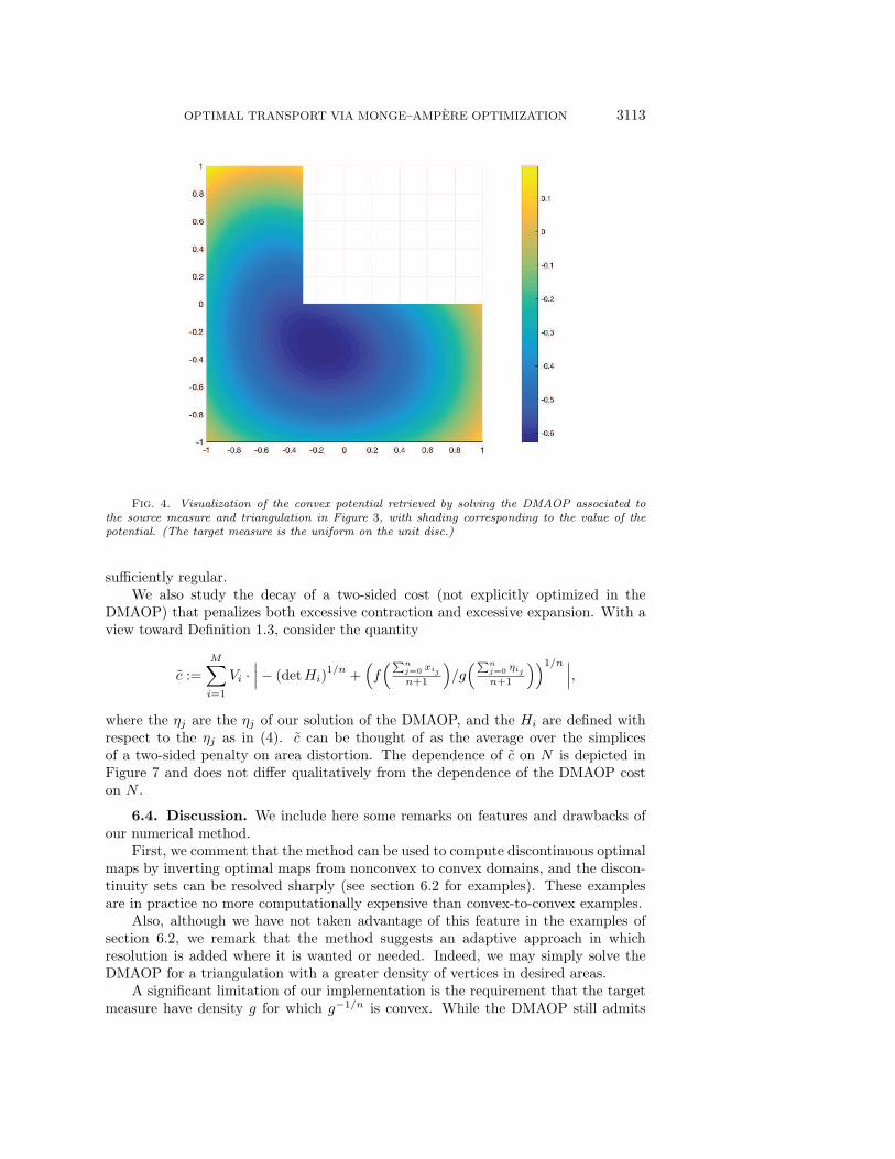
OPTIMAL TRANSPORT VIA MONGE–AMPERE OPTIMIZATION 3113
Fig. 4. Visualization of the convex potential retrieved by solving the DMAOP associated tothe source measure and triangulation in Figure 3, with shading corresponding to the value of thepotential. (The target measure is the uniform on the unit disc.)
sufficiently regular.We also study the decay of a two-sided cost (not explicitly optimized in the
DMAOP) that penalizes both excessive contraction and excessive expansion. With aview toward Definition 1.3, consider the quantity
c :=M∑i=1
Vi ·∣∣∣− (detHi)
1/n +(f(∑n
j=0 xijn+1
)/g(∑n
j=0 ηijn+1
))1/n ∣∣∣,where the ηj are the ηj of our solution of the DMAOP, and the Hi are defined withrespect to the ηj as in (4). c can be thought of as the average over the simplicesof a two-sided penalty on area distortion. The dependence of c on N is depicted inFigure 7 and does not differ qualitatively from the dependence of the DMAOP coston N .
6.4. Discussion. We include here some remarks on features and drawbacks ofour numerical method.
First, we comment that the method can be used to compute discontinuous optimalmaps by inverting optimal maps from nonconvex to convex domains, and the discon-tinuity sets can be resolved sharply (see section 6.2 for examples). These examplesare in practice no more computationally expensive than convex-to-convex examples.
Also, although we have not taken advantage of this feature in the examples ofsection 6.2, we remark that the method suggests an adaptive approach in whichresolution is added where it is wanted or needed. Indeed, we may simply solve theDMAOP for a triangulation with a greater density of vertices in desired areas.
A significant limitation of our implementation is the requirement that the targetmeasure have density g for which g−1/n is convex. While the DMAOP still admits

3114 MICHAEL LINDSEY AND YANIR A. RUBINSTEIN
Fig. 5. Visualization of numerical solution of the dynamical optimal transport problem withsource measure taken to be uniform and supported on the domain in the upper left and target measuretaken to be uniform on the unit disc. Times t = 0, 1
3 , 23 , 1 are depicted at upper left, upper right,
lower left, and lower right, respectively.
a minimizer for general target measures, it is only clear a priori that the DMAOPcan be practically solved when it is convex. We propose a remedy for this issue insection 8.
Another limitation is that the method is only first-order accurate. This is con-firmed empirically in section 6.3, but it is also to be expected due to the use offirst-order finite difference quotients in the definition (4) of the Hi in terms of thesubgradients ηj . One might hope to replace these with higher-order difference quo-tients, and indeed we will do this in section 7.
Lastly, the quadratic growth of run time in N is a major drawback. This growthis due to to the quadratic increase in the number of constraints of the DMAOP. Themodification introduced in section 7 will also address this issue.
7. Improving the efficiency and accuracy of the DMAOP. As remarkedabove, the quadratic growth of the problem size of the DMAOP in the number ofdiscretization points all but disqualifies it from competitive use in application. Thequadratic growth of the problem size derives from our global enforcement of the con-vexity of the potential. One might hope that this issue could be remedied by insteadrelying on a constraint that enforces convexity while relying only on local (second-derivative) information. Moreover, one might hope that the first-order accuracy ofthe scheme could be improved.
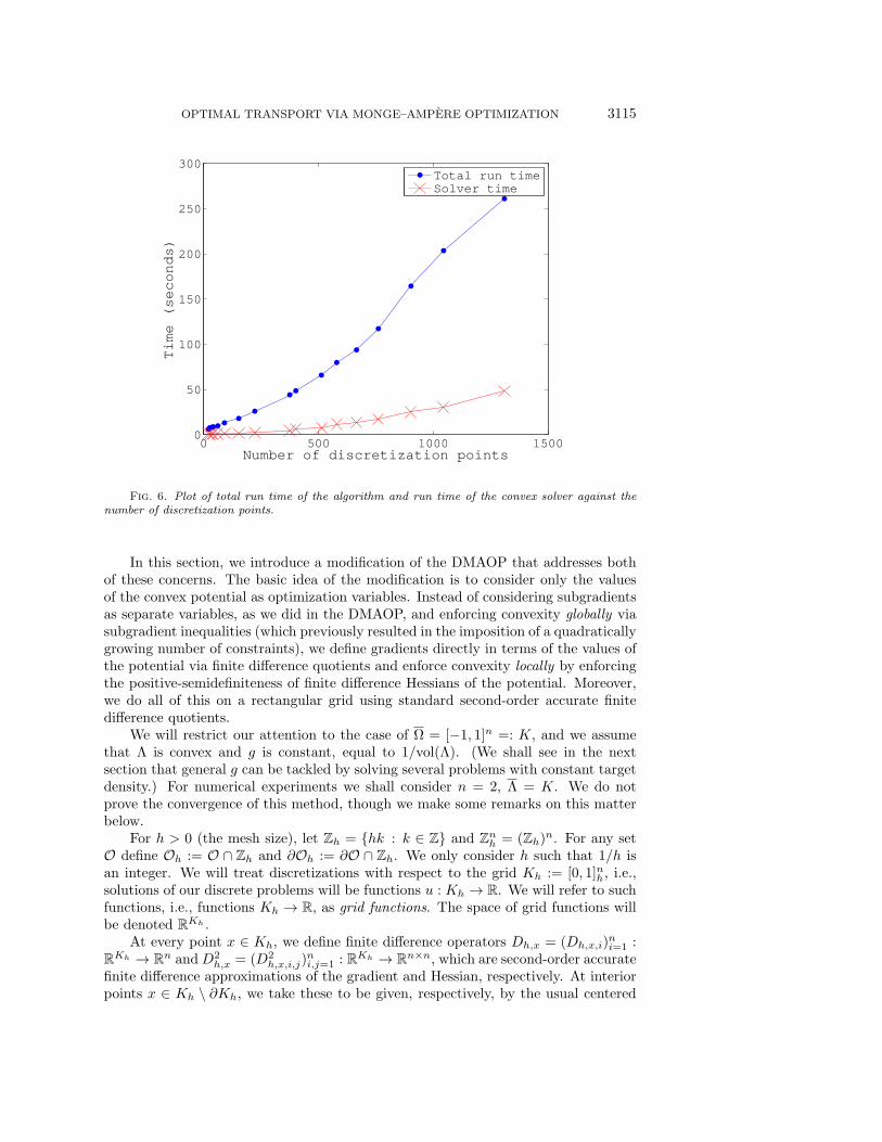
OPTIMAL TRANSPORT VIA MONGE–AMPERE OPTIMIZATION 3115
0 500 1000 15000
50
100
150
200
250
300
Number of discretization points
Time (seconds)
Total run time
Solver time
Fig. 6. Plot of total run time of the algorithm and run time of the convex solver against thenumber of discretization points.
In this section, we introduce a modification of the DMAOP that addresses bothof these concerns. The basic idea of the modification is to consider only the valuesof the convex potential as optimization variables. Instead of considering subgradientsas separate variables, as we did in the DMAOP, and enforcing convexity globally viasubgradient inequalities (which previously resulted in the imposition of a quadraticallygrowing number of constraints), we define gradients directly in terms of the values ofthe potential via finite difference quotients and enforce convexity locally by enforcingthe positive-semidefiniteness of finite difference Hessians of the potential. Moreover,we do all of this on a rectangular grid using standard second-order accurate finitedifference quotients.
We will restrict our attention to the case of Ω = [−1, 1]n =: K, and we assumethat Λ is convex and g is constant, equal to 1/vol(Λ). (We shall see in the nextsection that general g can be tackled by solving several problems with constant targetdensity.) For numerical experiments we shall consider n = 2, Λ = K. We do notprove the convergence of this method, though we make some remarks on this matterbelow.
For h > 0 (the mesh size), let Zh = hk : k ∈ Z and Znh = (Zh)n. For any setO define Oh := O ∩ Zh and ∂Oh := ∂O ∩ Zh. We only consider h such that 1/h isan integer. We will treat discretizations with respect to the grid Kh := [0, 1]nh, i.e.,solutions of our discrete problems will be functions u : Kh → R. We will refer to suchfunctions, i.e., functions Kh → R, as grid functions. The space of grid functions willbe denoted RKh .
At every point x ∈ Kh, we define finite difference operators Dh,x = (Dh,x,i)ni=1 :RKh → Rn and D2
h,x = (D2h,x,i,j)
ni,j=1 : RKh → Rn×n, which are second-order accurate
finite difference approximations of the gradient and Hessian, respectively. At interiorpoints x ∈ Kh \ ∂Kh, we take these to be given, respectively, by the usual centered
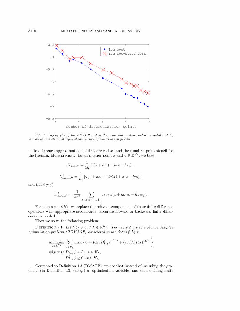
3116 MICHAEL LINDSEY AND YANIR A. RUBINSTEIN
3 4 5 6 7
Number of discretization points
-5.5
-5
-4.5
-4
-3.5
-3
-2.5
Log cost
Log two-sided cost
Fig. 7. Log-log plot of the DMAOP cost of the numerical solution and a two-sided cost (c,introduced in section 6.3) against the number of discretization points.
finite difference approximations of first derivatives and the usual 3n-point stencil forthe Hessian. More precisely, for an interior point x and u ∈ RKh , we take
Dh,x,iu =1
2h[u(x+ hei)− u(x− hei)] ,
D2h,x,i,iu =
1h2 [u(x+ hei)− 2u(x) + u(x− hei)] ,
and (for i 6= j)
D2h,x,i,ju =
14h2
∑σ1,σ2∈−1,1
σ1σ2 u(x+ hσ1ei + hσ2ej).
For points x ∈ ∂Kh, we replace the relevant components of these finite differenceoperators with appropriate second-order accurate forward or backward finite differ-ences as needed.
Then we solve the following problem.
Definition 7.1. Let h > 0 and f ∈ RKh . The revised discrete Monge–Ampereoptimization problem (RDMAOP) associated to the data (f, h) is
minimizeψ∈RKh
∑x∈Kh
max
0,−(detD2
h,xψ)1/n
+ (vol(Λ)f(x))1/n
subject to Dh,xψ ∈ K, x ∈ Kh,
D2h,xψ ≥ 0, x ∈ Kh.
Compared to Definition 1.3 (DMAOP), we see that instead of including the gra-dients (in Definition 1.3, the ηj) as optimization variables and then defining finite

OPTIMAL TRANSPORT VIA MONGE–AMPERE OPTIMIZATION 3117
difference Hessians in terms of these variables, the RDMAOP instead defines bothgradients and Hessians directly in terms of the grid function potential ψ, the onlyoptimization variable. Moreover, the convexity of ψ is enforced locally. We remarkthat convexity could alternatively be enforced via more sophisticated methods, inparticular via the wide stencil finite differences of Oberman [26], but this does notseem to be needed in the examples we consider (since the forward optimal transportmaps are C1).
7.1. Theoretical remarks on convergence. Although (as we will confirm be-low) this method is more efficient and more accurate than the DMAOP, the DMAOPlends itself more naturally to a convergence proof because it allows for the simpleconstruction of optimization potentials that are bona fide convex functions on Rn.By contrast, it is not clear how to extract a convex function defined on Rn from agrid function with positive semidefinite discrete Hessians (or even from a grid func-tion that is convex in the wide stencil sense of [26]). Thus the major missing piecein a convergence proof for the RDMAOP is a way of extracting convex potentialsfrom the grid functions retrieved by the optimization. We conjecture that this can bedone, but our working proof involves new ideas that take us too far afield from theanalysis in this paper and which are applicable more widely in the numerical analysisfor nonlinear elliptic PDEs. For these reasons, a full theoretical investigation of theconvergence of the RDMAOP will be the subject of future work.
7.2. Numerical experiments. We remark that the RDMAOP is a second-order cone program. We call MOSEK directly to solve it numerically. The numericalresults of this section were performed on a 2015 MacBook Pro with a 2.5 GHz IntelCore i7 processor.
First we consider a nontrivial example (see [5]) for which an explicit solution isavailable. To maintain consistency with [5], we will consider Ω = Λ = (−0.5, 0.5)2,though of course our discussion can be transferred by scaling to the domain (−1, 1)2
in order to fit into the framework described above.Define
q(z) =(− 1
8πz2 +
1256π3 +
132π
)cos(8πz) +
132π2 z sin(8πz),
and in turn define the source density
(98)f(x1, x2) = 1 + 4(q′′(x1)q(x2) + q(x1)q′′(x2))
+ 16(q(x1)q(x2)q′′(x1)q′′(x2)− q′(x1)2q′(x2)2)
on (−0.5, 0.5)2. The corresponding OT problem (with target density uniform on(−0.5, 0.5)2) admits the explicit solution
ϕx1(x1, x2) = x1 + 4q′(x1)q(x2), ϕx2(x1, x2) = x2 + 4q(x1)q′(x2).
The source density and the image of the grid Kh under the computed transportmap with h = 1/64 are shown in Figure 8.
Detailed numerical results (for the rescaled problem) are recorded in Table 1. Weobserve error on the order of h2, consistent with the second-order accuracy of thescheme, as well as linear growth in computational time with respect to the number ofdiscretization points. (Note that the number of discretization points is on the order ofh−2 since we are working in dimension 2.) We record separately the time taken by an

3118 MICHAEL LINDSEY AND YANIR A. RUBINSTEIN
0.5
1
0.5
1
0
1
0.5-0.5
0
1.5
-0.5
-1-1
2
Fig. 8. The source density defined by (98), after rescaling to (−1, 1)2, and the image of Kh
under the computed transport map (h = 1/64).
Table 1RDMAOP results for the OT problem defined by the source density of (98). Errors refer to
error of the transport (i.e., gradient) map. Nx denotes the number of discretization points along asingle dimension. Thus the number of optimization variables is N2
x . “On. time” and “Off. time”refer to the times taken by the online and offline parts of the computation, respectively.
h Nx L∞ error L2 error On. time (s) Off. time (s)
2−3 17 0.0324 0.0124 1.53 0.722−4 33 0.0022 0.0010 1.38 0.152−5 65 0.0010 0.0005 2.15 0.112−6 129 0.0003 0.0002 8.20 1.062−7 257 0.0002 0.0001 38.58 3.18
offline computational step, general to all RDMAOPs on a given grid (i.e., independentof source density), in which finite difference operators are constructed for the grid.
The reader can compare this example directly to [5]. (We remark that scalinghas been considered so that direct comparison of performance via Table 1 is indeedappropriate.) The run times for given problem sizes are quite similar, and the errorof our method is smaller, likely due to the higher order of accuracy.
We next consider the OT problem with source density
(99) f(x) = e− 1
2(1.4)2|x|2(3 + sin(8πx1) sin(6πx2)),
normalized to define a probability measure. The source density and the image of thegrid Kh under the computed transport map with h = 1/64 are shown in Figure 9.
We record numerical results in Table 2. We do not have an exact solution againstwhich to compare our numerical solution, so we measure the error of our numericalsolution for given h = 2−k by comparing it against the numerical solution for h =2−(k+1), subsampled on the grid of size 2−k. Again we observe error of order h2
and linear growth of computational time with respect to the number of discretizationpoints.

OPTIMAL TRANSPORT VIA MONGE–AMPERE OPTIMIZATION 3119
0
1
20
40
0.5 1
60
0.50
80
0
100
-0.5-0.5
-1 -1
Fig. 9. The source density defined by (99) and the image of Kh under the computed transportmap (h = 1/64).
Table 2RDMAOP results for the OT problem defined by the source density of (99). Errors refer to
error of the transport (i.e., gradient) map. Error for a given h = 2−k is measured by comparingagainst the computed solution for h = 2−(k+1). Nx denotes the number of discretization pointsalong a single dimension. Thus the number of optimization variables is N2
x .
h Nx L∞ error L2 error On. time (s) Off. time (s)
2−3 17 0.0375 0.0179 1.27 0.582−4 33 0.0119 0.0049 1.51 0.112−5 65 0.0034 0.0012 1.90 0.102−6 129 0.0013 0.0007 9.51 0.402−7 257 – – 42.31 3.13
8. Removing the restriction on the target measure. We propose a methodfor solving a given OT problem with general target density by solving a sequence ofOT problems with constant target densities. This approach amounts to a fixed pointiteration and is inspired by the Ricci iteration in differential geometry [35, 36], wherea similar approach for solving complex Monge–Ampere equations is introduced. Wemake no attempt at rigor in the following argument.
Suppose that Λ is convex as above, and let the target measure be given by g dxon its support Λ. Let V = vol(Λ), so the constant density 1/V defines the uniformprobability measure on Λ.
Recall that we want to solve (in some sense)
(100)det(∇2ϕ(x)
)=
f(x)g (∇ϕ(x))
, x ∈ Ω,
∇ϕ(Ω) = Λ.
Note that the solution ϕ of this problem simultaneously solves an OT problem with
3120 MICHAEL LINDSEY AND YANIR A. RUBINSTEIN
source density
(101)f/(g ∇ϕ)∫
Ω f/(g ∇ϕ) dx=
f/(g ∇ϕ)∫Ω det (∇2ϕ(x)) dx
=f/(g ∇ϕ)
V
and constant target density 1/V .Keeping this fact in mind, we turn to defining our iterative procedure. Let f (0) =
f , and let ϕ(0) be the solution of
det(∇2ϕ(x)
)= V f (0)(x), x ∈ Ω,
∇ϕ(Ω) = Λ,
i.e., the original OT problem with the target measure replaced by the uniform measureon Λ. We then define f (1)(x) := f(x)/g(∇ϕ(0)(x)), set f (1) := f (1)/
( ∫Ω f
(1) dx), and
solve another OT problem with source density f (1) and uniform target measure. Thisiteration can be repeated many times.
More precisely, we define ϕ(i+1) to be the solution of
det(∇2ϕ(x)
)= V f (i+1)(x) x ∈ Ω,
∇ϕ(Ω) = Λ,
where f (i+1) := f (i+1)/( ∫
Ω f(i+1) dx
)for f (i+1) := f/(g ∇ϕ(i)).
Note from our argument above (in particular, (101)) that the solution of (100) isa fixed point of this iteration.
Suppose that ϕ(i) converges to some ϕ as i → ∞ in some suitably strong sense.Then we expect that ϕ is a fixed point and hence solves (100). We do not provesuch convergence (and remark that it is not at all obvious to us how to do so), butwe observe below that rapid convergence occurs in practice, at least with densitiesbounded away from zero.
8.1. Numerical implementation of the iteration. We consider the samesetting as in section 7 but now allow g to be nonconstant. We fix some mesh sizeh > 0 for the entirety of the iterative procedure. We inductively define ψ(i) ∈ RKh tobe a grid function solving the RDMAOP associated to the data (f (i), h) (see Definition7.1), where f (i) := f (i)/I
[f (i)]
for f (i)(x) := f(x)/g(Dh,xψ(i−1)) and for I an operator
on grid functions that approximates the integral over K. In particular, for u a gridfunction, we take I[u] to return the true integral of the function that is constant oneach grid cube, with its value on a given grid cube equal to the average of u overthe vertices of the cube. We terminate iteration when the L2 distance between twoconsecutive solutions first drops below h2/2.
8.2. Numerical experiments. Consider once again the source density of (98)and (unnormalized) target density
(102) g(x) := 3 + sin(3πx1) sin(2πx2).
The source density and the image of the grid Kh under the computed transportmap with h = 1/64 are shown in Figure 10.
Detailed numerical results are recorded in Table 3. Once again we do not havean exact solution against which to compare our numerical solution, so we measurethe error for h = 2−k by comparing against the result for h = 2−(k+1). Once againwe observe error of order h2 and linear growth of computational time with respect to

OPTIMAL TRANSPORT VIA MONGE–AMPERE OPTIMIZATION 3121
2
1
2.5
0.5
3
0
1-0.5
3.5
0.5
0
-0.5-1
4
-1
Fig. 10. The target density defined by (102) and the image of Kh under the computed transportmap (h = 1/64), with source density as in Figure 8.
Table 3RDMAOP results for the OT problem defined by the source density of (98) and the target
density of (102). Errors refer to error of the transport (i.e., gradient) map. Error for a givenh = 2−k is measured by comparing against the computed solution for h = 2−(k+1).
h L∞ error L2 error Iterations On. time (s) Off. time (s)
2−3 0.0814 0.0317 3 3.36 0.592−4 0.0175 0.0095 4 5.59 0.092−5 0.0056 0.0031 4 8.97 0.092−6 0.0017 0.0008 5 45.16 0.402−7 – – 5 207.02 3.08
the number of discretization points. The number of iterations needed to reach a fixedpoint does not appear to depend strongly on h.
Next we consider an example in which the iterative method does not perform aswell as one might hope. Define (unnormalized) source and target densities by
(103) f = 1.5− 1B(0,0.5)
and
(104) g(x) = 6 + 25∑
x′1,x′2∈−1,1
e− 1
2(0.2)2|x−(x′1,x
′2)|2
.
The target density and the image of the grid Kh under the computed transportmap with h = 1/64 are shown in Figure 11.
Results are recorded in Table 4. This time we observe observe error of order h,though still linear growth of computational time. This outcome seems to be typicalfor the iterative procedure when the target density is close to zero on a large portionof the target domain. Indeed, the iterative procedure completely fails to convergenumerically in many situations with highly degenerate target densities. It is not clear

3122 MICHAEL LINDSEY AND YANIR A. RUBINSTEIN
5
1
10
15
0.5 1
20
25
0.50
30
0
35
-0.5-0.5
-1 -1
Fig. 11. The target density defined by (104) and the image of Kh under the computed transportmap (h = 1/64), with source density as in Figure 103.
Table 4RDMAOP results for the OT problem defined by the source density of (103) and the target
density of (104). Errors refer to error of the transport (i.e., gradient) map. Error for a givenh = 2−k is measured by comparing against the computed solution for h = 2−(k+1).
h L∞ error L2 error Iterations On. time (s) Off. time (s)
2−3 0.0312 0.0192 6 7.42 0.632−4 0.0156 0.0069 7 10.53 0.102−5 0.0091 0.0041 7 14.11 0.122−6 0.0045 0.0025 9 78.90 0.382−7 – – 10 381.73 3.11
to the authors whether this shortcoming is inherent in the method or whether it canbe overcome with more stable fixed point iteration techniques.
9. Future directions. First, it is an interesting open question whether ourconvergence proof can be upgraded to yield error bounds.
Second, we plan to follow up on the remarks of section 7.1 regarding the essentialdifficulties of proving convergence for the RDMAOP.
Third, the theoretical and numerical convergence properties of the fixed point it-eration of section 7 remain open, as does the possibility of a better numerical approachto the fixed point iteration.
Acknowledgments. The authors are grateful to O. Chodosh, V. Jain, andL. Panchev for many stimulating discussions and initial collaboration on this projectand on [11]. We also thank the anonymous referees for many helpful comments.
REFERENCES
[1] S. Angenent, S. Haker, and A. Tannenbaum, Minimizing flows for the Monge–Kantorovich problem, SIAM J. Math. Anal., 35 (2003), pp. 61–97, https://doi.org/10.1137/S0036141002410927.
OPTIMAL TRANSPORT VIA MONGE–AMPERE OPTIMIZATION 3123
[2] A. Bagh and R. J.-B. Wets, Convergence of set-valued mappings: Equi-outer semicontinuity,Set-Valued Anal., 4 (1996), pp. 333–360.
[3] A. Baldes and O. Wohlrab, Computer graphics of solutions of the generalized Monge–Ampere equation, in Geometric Analysis and Computer Graphics (Berkeley, CA, 1988),Math. Sci. Res. Inst. Publ. 17, Springer, New York, 1991, pp. 19–30.
[4] J.-D. Benamou and Y. Brenier, A computational fluid mechanics solution to the Monge-Kantorovich mass transfer problem, Numer. Math., 84 (2000), pp. 375–393.
[5] J.-D. Benamou, B. D. Froese, and A. M. Oberman, Numerical solution of the optimaltransportation problem using the Monge–Ampere equation, J. Comput. Phys., 260 (2014),pp. 107–126.
[6] J.-D. Benamou, B. D. Froese, and A. M. Oberman, A Viscosity Solution Approach tothe Monge–Ampere Formulation of the Optimal Transportation Problem, preprint, https://arxiv.org/abs/1208.4873, 2012.
[7] S. Boyd and L. Vandenberghe, Convex Optimization, Cambridge University Press, Cam-bridge, uk, 2004.
[8] Y. Brenier, Polar factorization and monotone rearrangement of vector-valued functions,Comm. Pure Appl. Math., 44 (1991), pp. 375–417.
[9] L. Caffarelli, The regularity of mappings with a convex potential, J. Amer. Math. Soc., 5(1992), pp. 99–104.
[10] O. Chodosh, V. Jain, M. Lindsey, L. Panchev, and Y. A. Rubinstein, Visualizing optimaltransportation maps, abstracts of papers presented to the American Mathematical Society,Vol. 34, No. 1086-28-496, 2013.
[11] O. Chodosh, V. Jain, M. Lindsey, L. Panchev, and Y. A. Rubinstein, On discontinuity ofplanar optimal transport maps, J. Topology Anal., 7 (2015), pp. 239–260.
[12] C. K. Chui and P. W. Smith, A note on Landau’s problem for bounded intervals, Amer. Math.Monthly, 82 (1975), pp. 927–929.
[13] M. Cuturi, Sinkhorn distances: Lightspeed computation of optimal transportation distances,Neural Information Processing Systems Conference, 2013.
[14] X.-B. Feng, R. Glowinski, and M. Neilan, Recent developments in numerical methods forfully nonlinear second order partial differential equations, SIAM Rev., 55 (2013), pp. 205–267, https://doi.org/10.1137/110825960.
[15] B. D. Froese and A. M. Oberman, Convergent filtered schemes for the Monge–Ampere partialdifferential equation, SIAM J. Numer. Anal., 51 (2013), pp. 423–444, https://doi.org/10.1137/120875065.
[16] W. Gangbo and R. McCann, The geometry of optimal transportation, Acta Math., 177 (1996),pp. 113–161.
[17] K. Guittet, On the time-continuous mass transport problem and its approximation by aug-mented Lagrangian techniques, SIAM J. Numer. Anal., 41 (2003), pp. 382–399, https://doi.org/10.1137/S0036142901386069.
[18] E. Haber, T. Rehman, and A. Tannenbaum, An efficient numerical method for the solutionof the L2 optimal mass transfer problem, SIAM J. Sci. Comput., 32 (2010), pp. 197–211,https://doi.org/10.1137/080730238.
[19] J. Kitagawa, An iterative scheme for solving the optimal transportation problem, Calc. Var.Partial Differential Equations, 51 (2014), pp. 243–263.
[20] B. Levy, A numerical algorithm for L2 semi-discrete optimal transport in 3D, ESAIM Math.Model. Numer. Anal., 49 (2015), pp. 1693–1715.
[21] G. Loeper and F. Rapetti, Numerical solution of the Monge–Ampere equation by a Newton’salgorithm, C. R. Acad. Sci. Paris Ser. I, 340 (2005), pp. 319–324.
[22] J. Lofberg, YALMIP: A toolbox for modeling and optimization in MATLAB, in Proceedingsof the 2004 IEEE International Symposium on Computer Aided Control Systems Design,IEEE, 2004, https://doi.org/10.1109/CACSD.2004.1393890.
[23] Q. Merigot and E. Oudet, Discrete optimal transport: Complexity, geometry and applica-tions, Discrete Comput. Geom., 55 (2016), pp. 263–283.
[24] H. Minkowski, Volumen und Oberflachen, Math. Ann., 57 (1903), pp. 447–495.[25] MOSEK ApS, The MOSEK Optimization Toolbox for MATLAB Manual, Version 7.1 (Revision
28), http://docs.mosek.com/7.1/toolbox/index.html, 2015.[26] A. Oberman, Wide stencil finite difference schemes for the elliptic Monge-Ampere equation
and functions of the eigenvalues of the hessian, Discrete Contin. Dyn. Syst. Ser. B, 10(2008), pp. 221–238.
[27] A. Oberman and Y. Ruan, An Efficient Linear Programming Method for Optimal Trans-portation, preprint, https://arxiv.org/abs/1509.03668, 2015.
[28] V. I. Oliker and L. D. Prussner, On the numerical solution of the equation

3124 MICHAEL LINDSEY AND YANIR A. RUBINSTEIN
(∂2z/∂x2)(∂2z/∂y2) − ((∂2z/∂x∂y))2 = f and its discretizations. I, Numer. Math., 54(1988), pp. 271–293.
[29] N. Papadakis, G. Peyre, and E. Oudet, Optimal transport with proximal splitting, SIAM J.Imaging Sci., 7 (2014), pp. 212–238, https://doi.org/10.1137/130920058.
[30] P.-O. Persson and G. Strang, A simple mesh generator in MATLAB, SIAM Rev., 46 (2004),pp. 329–345, https://doi.org/10.1137/S0036144503429121.
[31] A. V. Pogorelov, The Minkowski Multidimensional Problem, Wiley, New York, 1978.[32] J. Rauch and B. A. Taylor, The Dirichlet problem for the multidimensional Monge–Ampere
equation, Rocky Mountain J. Math., 7 (1977), pp. 345–364.[33] R. T. Rockafellar, Convex Analysis, Princeton University Press, Princeton, NJ, 1970.[34] R. T. Rockafellar and R. J.-B. Wets, Variational Analysis, Springer, New York, 1997.[35] Y. A. Rubinstein, The Ricci iteration and its applications, C. R. Math. Acad. Sci. Paris, 345
(2007), pp. 445–448.[36] Y. A. Rubinstein, Some discretizations of geometric evolution equations and the Ricci iteration
on the space of Kahler metrics, Adv. Math., 218 (2008), pp. 1526–1565.[37] B. Schmitzer, A sparse multiscale algorithm for dense optimal transport, J. Math. Imaging
Vision, 56 (2016), pp. 238–259.[38] M. M. Sulman, J. F. Williams, and R. D. Russell, An efficient approach for the numerical
solution of the Monge–Ampere equation, Appl. Numer. Math., 61 (2011), pp. 298–307.[39] C. Villani, Topics in Optimal Transportation, AMS, Providence, RI, 2003.[40] C. Villani, Optimal Transport: Old and New, Springer, Berlin, 2009.[41] Z. Zahorski, Sur l’ensemble des points de non-derivabilite d’une fonction continue, Bull. Soc.
Math. France, 74 (1946), pp. 147–178.