Optimal Topology of Aircraft Rib and Spar Structures under Aeroelastic Loads

Bret K. Stanford1 NASA Langley Research Center, Hampton, VA, 23681

Peter D. Dunning2 National Institute of Aerospace, Hampton, VA, 23666

Several topology optimization problems are conducted within the ribs and spars of a wing box. It is desired to locate the best position of lightening holes, truss/cross-bracing, etc. A variety of aeroelastic metrics are isolated for each of these problems: elastic wing compliance under trim loads and taxi loads, stress distribution, and crushing loads. Aileron effectiveness under a constant roll rate is considered, as are dynamic metrics: natural vibration frequency and flutter. This approach helps uncover the relationship between topology and aeroelasticity in subsonic transport wings, and can therefore aid in understanding the complex aircraft design process which must eventually consider all these metrics and load cases simultaneously.

I. Introduction his work is concerned with improving the structural performance of a high aspect ratio subsonic transport wing via the use of topology optimization. An increased aspect ratio stems from a desire to decrease the induced-

drag of the wing (and thus improve key metrics like specific fuel consumption), but also results in a highly-flexible wing, potentially susceptible to onerous issues (static and dynamic) associated with the flight loading. Aeroelastic optimization of the internal wing structure can be used to obtain the best compromise between adequate structural reinforcement and added weight, which may lead to unconventional structural concepts. An unconventional result is particularly likely if topology optimization is utilized, wherein an optimizer makes fundamental decisions about the layout and connectivity of the structure in an effort to improve some design metric in a feasible manner.

Several different types of topological parameterizations for wing structures can be found in the literature. One method populates a wing box with a lattice of connecting members, and allows the optimizer to decide which of these members to remove. If these members are situated in an orthogonal pattern aligned with the wing’s leading edge, they may be designated as “ribs” and “spars”, as in the work of Wang et al. [1]. Broader parameterizations used by Balabanov and Haftka [2], Locatelli et al. [3], and Kobayashi et al. [4] highlight the usefulness of diagonally-oriented and/or curvilinear members, which blend the role of traditional rib and spar structures, and thus defy easy characterization. This type of topology is two-dimensional, in that the parameterization is defined in the plane of the wing, and each member is full-depth: it fully extends from the lower skins to the upper skins.

Alternatively, a three-dimensional parameterization may be considered, by populating the wing box with a large number of three-dimensional finite elements, and allowing the optimizer to decide which elements to remove. The resulting optimization problem is typically solved with SIMP-based methods (solid isotropic material with penalization), or level set methods. This parameterization is utilized in the work of Kim et al. [5] (at a single panel level, rather than a complete wing), James and Martins [6], and Dunning et al. [7]. The resulting structure typically bears no resemblance to traditional rib/spar networks, which may indicate one of two things. The first is that the appropriate physics, load cases, and/or constraint boundaries were not included in the optimization problem, and if they had been, the resulting topology would qualitatively approach a lattice of ribs and spars (which have been used almost exclusively in aircraft structures for decades [8]). The second is that the design problem was properly defined, and that the non-traditional topology may present an interesting new direction for efficient wing structures.

The approach taken in the current work is a compromise between the two parameterizations discussed above. A wing box is seeded with a pre-determined (and fixed) number of ribs and spars, each is discretized into a series of 1 Research Aerospace Engineer, Aeroelasticity Branch, bret.k.stanford@nasa.gov, AIAA Member. 2 Research Scholar, peter.d.dunning@nasa.gov, AIAA Member.

T

https://ntrs.nasa.gov/search.jsp?R=20140007307 2018-05-21T13:27:25+00:00Z

2

planar shell finite elements, and the optimizer decides which elements to remove. Though this method is restricted in that it acknowledges the typical rib/spar construction of aircraft wings, a significant amount of discretion is still provided to the optimizer, particularly if a dense network of members is included in the framework. Weight-saving cutouts may be added, spars may be reduced to stringers, ribs reduced to rib-caps or stiffeners, or members may be removed entirely. Precedent for this approach is found in Ref. [9], though that work struggles to find a crisp solid-void boundary within the ribs. Several authors find the optimal topology within a single representative rib (Eschenauer and Olhoff [10], Krog et al. [11], Maute and Reich [12], and Oktay et al. [13]) a single stiffener (Stanford and Beran [14]), or a series of stiffeners (Stanford et al. [15]).

It is important to note which portions of the wing structure are being optimized in this paper, and which are not. Topology optimization is conducted within the ribs, as well as any internal spars. Topology optimization could also be conducted within the leading and trailing edge spars, but a substantial quantity of mechanisms and structures are connected to these members (slats, spoilers, flaps, etc. [8]), and the loads they impart are undefined for the current conceptual design. Furthermore, the details of the fuel tanks may preclude holes in these structures. Topology optimization obviously cannot be conducted within the wing skins (though tailoring could be readily accomplished through thickness- and/or stiffness-based optimization [16]): these structures are completely unaltered for this work.

Given that these external structures bear a substantial portion of the bending and torsional flight loads, optimizing only the topology of the internal structures will produce a moderate improvement in flight metrics: 10-20% is typically demonstrated below. The topology optimization method discussed here is probably best viewed as a way to further reduce wing weight, after (or in parallel with) the optimization of the external wing box structures. Furthermore, the approach taken here is to obtain a variety of topologies, each of which is defined by a limited optimization problem (i.e., a wing topology that only considers the trade-off between weight and structural compliance, another for weight and flutter, etc.), rather than the multitude of physics and constraints that should be considered during comprehensive aircraft design. This approach can provide a better understanding of the relationship between various aeroelastic metrics and the distribution of material within a wing box, and therefore improve the understanding of the optimal topology when each of these metrics are eventually included in a unified aircraft design process. In this paper, a series of optimal topologies are divided into 3 categories: symmetric static aeroelasticity (section III), antisymmetric static aeroelasticity (section IV), and dynamic aeroelasticity (section V).

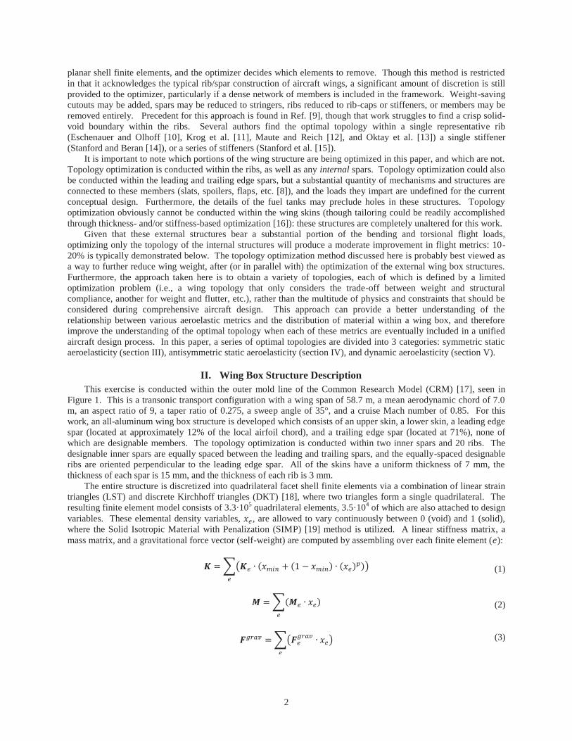
II. Wing Box Structure Description This exercise is conducted within the outer mold line of the Common Research Model (CRM) [17], seen in

Figure 1. This is a transonic transport configuration with a wing span of 58.7 m, a mean aerodynamic chord of 7.0 m, an aspect ratio of 9, a taper ratio of 0.275, a sweep angle of 35°, and a cruise Mach number of 0.85. For this work, an all-aluminum wing box structure is developed which consists of an upper skin, a lower skin, a leading edge spar (located at approximately 12% of the local airfoil chord), and a trailing edge spar (located at 71%), none of which are designable members. The topology optimization is conducted within two inner spars and 20 ribs. The designable inner spars are equally spaced between the leading and trailing spars, and the equally-spaced designable ribs are oriented perpendicular to the leading edge spar. All of the skins have a uniform thickness of 7 mm, the thickness of each spar is 15 mm, and the thickness of each rib is 3 mm.

The entire structure is discretized into quadrilateral facet shell finite elements via a combination of linear strain triangles (LST) and discrete Kirchhoff triangles (DKT) [18], where two triangles form a single quadrilateral. The resulting finite element model consists of 3.3·105 quadrilateral elements, 3.5·104 of which are also attached to design variables. These elemental density variables, , are allowed to vary continuously between 0 (void) and 1 (solid), where the Solid Isotropic Material with Penalization (SIMP) [19] method is utilized. A linear stiffness matrix, a mass matrix, and a gravitational force vector (self-weight) are computed by assembling over each finite element ( ):

(1)

(2)

(3)

3

where is an elemental stiffness matrix associated with solid elements, is a small non-zero number, and is a penalization factor (typically greater than 2), is the elemental mass matrix associated with solid elements, and

is an elemental gravitational force vector associated with solid elements. The interpolation scheme used in Eq. 1 is intended to prevent unbounded displacements of void elements under self-weight [20], and to prevent localized vibration modes in these areas.

Figure 1. Proposed wing box within the Common Research Model [17].

III. Symmetric Static Aeroelasticity The term “symmetric” as used here indicates that the lift distribution is identical between the left and the right

wings: steady forward flight. The elastic deformation of a wing is computed by:

(4)

where the solution vector has six degrees of freedom (three displacements and three rotations) per node, and is the load factor (equal to 1 for steady level flight). Aerodynamic forces are computed with the assumption of a flat-plate lifting surface via the doublet lattice method [21]. The pressure-downwash equation is given by: (5) where is the influence matrix (the superscript indicates a symmetric aerodynamic condition about the centerline of the airplane), and is a vector of differential pressure coefficients acting on each box. Three factors contribute to the downwash at the center of each box: the slope of the airfoil’s centerline (due to built-in camber and twist), the angle of attack at the root of the wing (where is a vector of ones), and additional wing twist from the elastic deformation . The interpolation matrix is derived from a finite plate spline [22], a method that uses a plate finite element model to transfer information from the wing box to the aerodynamic lattice in a work-equivalent manner.

Aerodynamic forces are subsequently computed as: (6) where is the dynamic pressure and is a second interpolation matrix, also derived from a finite plate spline. The total aerodynamic lift over a single wing is constrained to meet a trim condition:

(7)

is a vector of the area of each box, and is the total weight of half of the aircraft. is the sum of the wing weight (which will change during the optimization process) and some predetermined and fixed weight of the remainder of the aircraft. Additional aerodynamics and pitch-based trim requirements from a tail are ignored for this work. The final aeroelastic equations are given as:

4

(8)

where the angle of attack of the wing is constantly altered to maintain trim [23].

The aeroelastic unknowns can be computed by simply solving Eq. 8 as written, by re-writing the aerodynamic terms as a function of (via an aerodynamic stiffness matrix), or by simply iterating between the structural (Eq. 4) and aerodynamic equations (Eqs. 5 and 7). This latter option is used here, as the sparsity of is preserved, which can be factored a single time prior to iterating. This analysis framework is developed as an in-house MATLAB (a product of Mathworks Inc. ) code, which has been extensively verified for accuracy against NASTRAN’s (a product of MSC Software*) static aeroelastic solvers.

A. Aeroelastic Compliance The first topology optimization problem seeks to minimize the compliance of the wing deformation:

(9)

where the elemental design variables are grouped into the vector , which is then passed through a linearly-decaying cone-shape filter [19] to obtain the variable densities . Side constraints and a volume fraction constraint are also imposed. The volume fraction constraint specifies the percentage of designable material which must be retained. Because the entire structure is made from the same aluminum material, setting effectively sets the wing mass as well. Though wing optimization problems are typically written to minimize the mass (Ref. [9], for example), here wing mass (or volume fraction, explicitly) is set as a constraint, in keeping with the standard SIMP formulation [19].

It is noted that only , , and are functions of the design variables, and gradients of the structural compliance with respect to are easily computed with the adjoint method [24]. Optimal topologies are found with the method of moving asymptotes [25].

The load factor is set to 1, the dynamic pressure is 5897 N/m2, and the Mach number is 0.85. The fixed weight of the aircraft is 500 kN, thus is equal to 250 kN plus the weight of one wing (wing weight is typically 25-30% of the total aircraft weight for these cases). The minimum density is set to 0.001, is set to 3, and the volume constraint is set to 0.5 (i.e., the optimizer must retain 50% of the designable ribs and spars in Figure 1). The lower and upper layers of elements on each rib and spar are fixed as solid elements ( = 1). For the spars, this constraint acknowledges that, even if the optimizer completely removes a spar in a certain area, some local stiffness is desired to prevent skin buckling (a metric which the optimizer is unaware of), and so a stringer-like structure is always left behind. Similar arguments can be made for rib-caps and stiffeners if a rib is completely removed. Furthermore, the permanently-solid upper layer of each rib also recognizes the non-structural role of each rib station to maintain the outer mold line of the upper and lower skins [8][11].

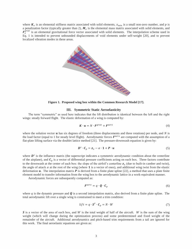
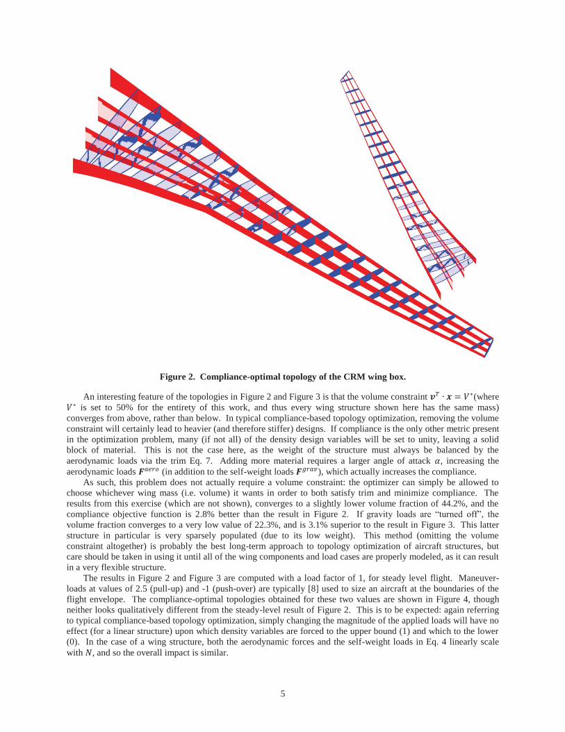
The optimal result of Eq. 9 is shown in Figure 2, where two views of the same structure are provided. Towards the root of the wing, the optimizer removes the inner material from each of the spars (as the bending stresses will be highest along the outer fibers), and creates a series of cross-braced trusses within some of the ribs. Towards the wing tip, however, the optimizer fully populates each rib and spar. This may seem to be an unusual result, as the stresses at the wing tip will be relatively small, and so adding material in this area would not typically be the best way to exploit the conflict between wing mass and compliance in Eq. 9. The self-weight loads are driving this topology, in part: adding downward gravitational loads at the wing tip will help offset (via inertial relief) the upwards aerodynamic loads , decreasing the total bending moment (and therefore the total compliance). This is confirmed by re-running the topology optimization without in Eq. 8 (the term is still included in the trim equation), where the final structure is seen in Figure 3. The result is as expected, with the majority of the outboard ribs removed, and cross-bracing adding to the spars towards the tip. This exploitation of inertial relief has been noted before [26], and will be discussed in later sections.

The use of trademarks or names of manufacturers in this report is for accurate reporting and does not constitute and official endorsement, either

expressed or implied, of such products or manufacturers by the National Aeronautics and Space Administration.

5

Figure 2. Compliance-optimal topology of the CRM wing box.

An interesting feature of the topologies in Figure 2 and Figure 3 is that the volume constraint (where is set to 50% for the entirety of this work, and thus every wing structure shown here has the same mass)

converges from above, rather than below. In typical compliance-based topology optimization, removing the volume constraint will certainly lead to heavier (and therefore stiffer) designs. If compliance is the only other metric present in the optimization problem, many (if not all) of the density design variables will be set to unity, leaving a solid block of material. This is not the case here, as the weight of the structure must always be balanced by the aerodynamic loads via the trim Eq. 7. Adding more material requires a larger angle of attack , increasing the aerodynamic loads (in addition to the self-weight loads ), which actually increases the compliance.

As such, this problem does not actually require a volume constraint: the optimizer can simply be allowed to choose whichever wing mass (i.e. volume) it wants in order to both satisfy trim and minimize compliance. The results from this exercise (which are not shown), converges to a slightly lower volume fraction of 44.2%, and the compliance objective function is 2.8% better than the result in Figure 2. If gravity loads are “turned off”, the volume fraction converges to a very low value of 22.3%, and is 3.1% superior to the result in Figure 3. This latter structure in particular is very sparsely populated (due to its low weight). This method (omitting the volume constraint altogether) is probably the best long-term approach to topology optimization of aircraft structures, but care should be taken in using it until all of the wing components and load cases are properly modeled, as it can result in a very flexible structure.

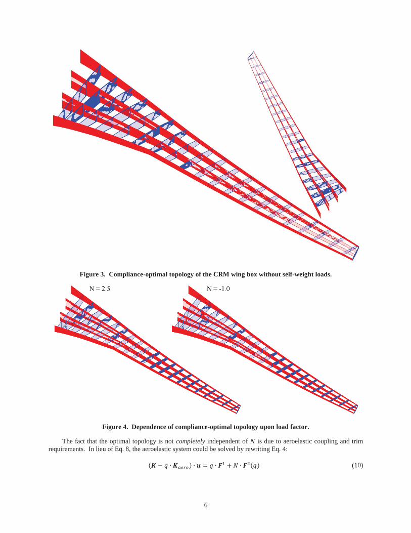
The results in Figure 2 and Figure 3 are computed with a load factor of 1, for steady level flight. Maneuver-loads at values of 2.5 (pull-up) and -1 (push-over) are typically [8] used to size an aircraft at the boundaries of the flight envelope. The compliance-optimal topologies obtained for these two values are shown in Figure 4, though neither looks qualitatively different from the steady-level result of Figure 2. This is to be expected: again referring to typical compliance-based topology optimization, simply changing the magnitude of the applied loads will have no effect (for a linear structure) upon which density variables are forced to the upper bound (1) and which to the lower (0). In the case of a wing structure, both the aerodynamic forces and the self-weight loads in Eq. 4 linearly scale with , and so the overall impact is similar.

6

Figure 3. Compliance-optimal topology of the CRM wing box without self-weight loads.

Figure 4. Dependence of compliance-optimal topology upon load factor.

The fact that the optimal topology is not completely independent of is due to aeroelastic coupling and trim requirements. In lieu of Eq. 8, the aeroelastic system could be solved by rewriting Eq. 4:

(10)

7

where the forcing functions on the right side of Eq. 10 can be derived from the built-in wing camber , the angle of attack (constantly altered to meet trim), and the self-weight loading. is an aerodynamic stiffness matrix. The solution to Eq. 10 will be the same as Eq. 8, but Eq. 10 is not used here because is a large fully-populated matrix, as it involves inverting . If was a proportional constant for both forcing functions, then the optimal topology would be completely independent of , but it is not: the first term is not impacted by . The second forcing term is larger in magnitude than the first, and so the dependence on load factor is weak, as seen in Figure 4.

One obvious issue with many of the topologies shown to this point is that the optimizer, in many cases, removes most (or all) of the material in many of the ribs. A potential reason for this is that a main role of each rib structure is to maintain the intended airfoil shape of the upper and lower skins (outer mold line) [11]. The optimizer knows nothing of this role, being solely concerned with weight and elastic compliance. This effect will be difficult to account for with the flat-plate aerodynamic tool used here. Only differential pressure distributions are computed, rather than individual upper and lower surface pressures, which will lead to OML distortions. Two methods are explored here to circumvent the problem. First, crushing Brazier loads may be included in the load set, which is discussed below (section III-E).

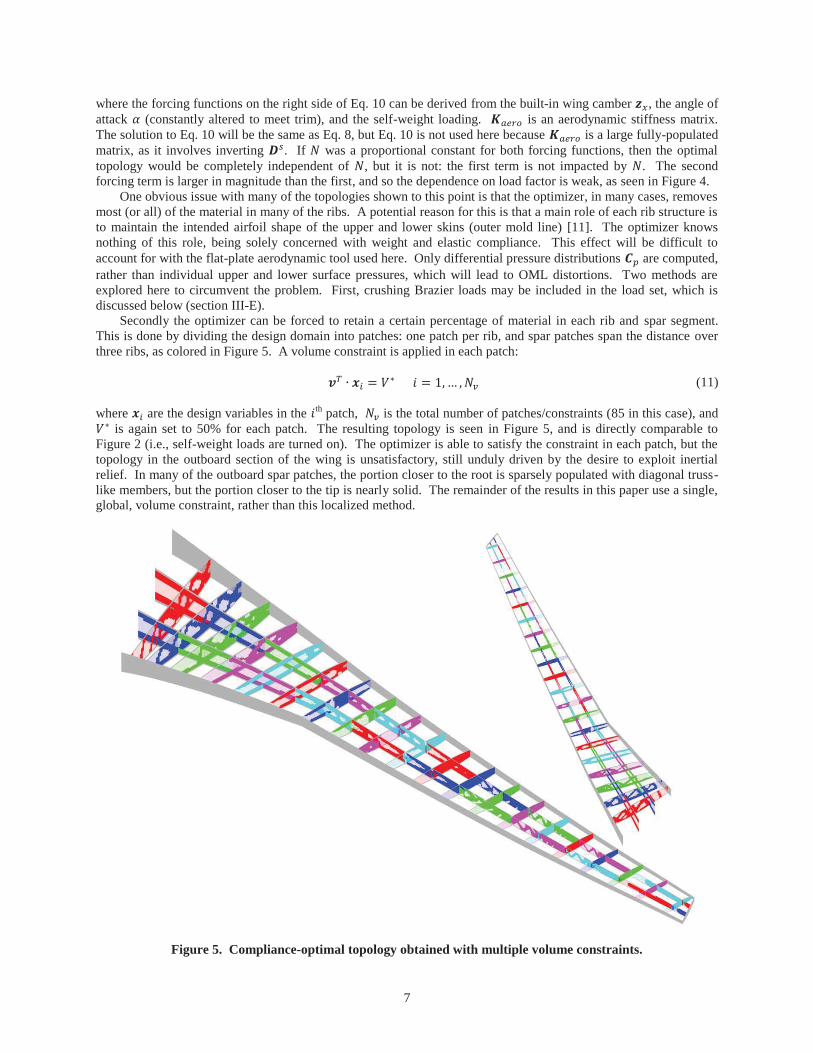
Secondly the optimizer can be forced to retain a certain percentage of material in each rib and spar segment. This is done by dividing the design domain into patches: one patch per rib, and spar patches span the distance over three ribs, as colored in Figure 5. A volume constraint is applied in each patch: (11) where are the design variables in the th patch, is the total number of patches/constraints (85 in this case), and

is again set to 50% for each patch. The resulting topology is seen in Figure 5, and is directly comparable to Figure 2 (i.e., self-weight loads are turned on). The optimizer is able to satisfy the constraint in each patch, but the topology in the outboard section of the wing is unsatisfactory, still unduly driven by the desire to exploit inertial relief. In many of the outboard spar patches, the portion closer to the root is sparsely populated with diagonal truss-like members, but the portion closer to the tip is nearly solid. The remainder of the results in this paper use a single, global, volume constraint, rather than this localized method.

Figure 5. Compliance-optimal topology obtained with multiple volume constraints.

8

B. Taxi Bumps One method of preventing the optimizer’s desire to add mass outboard for inertial relief is to include a taxi

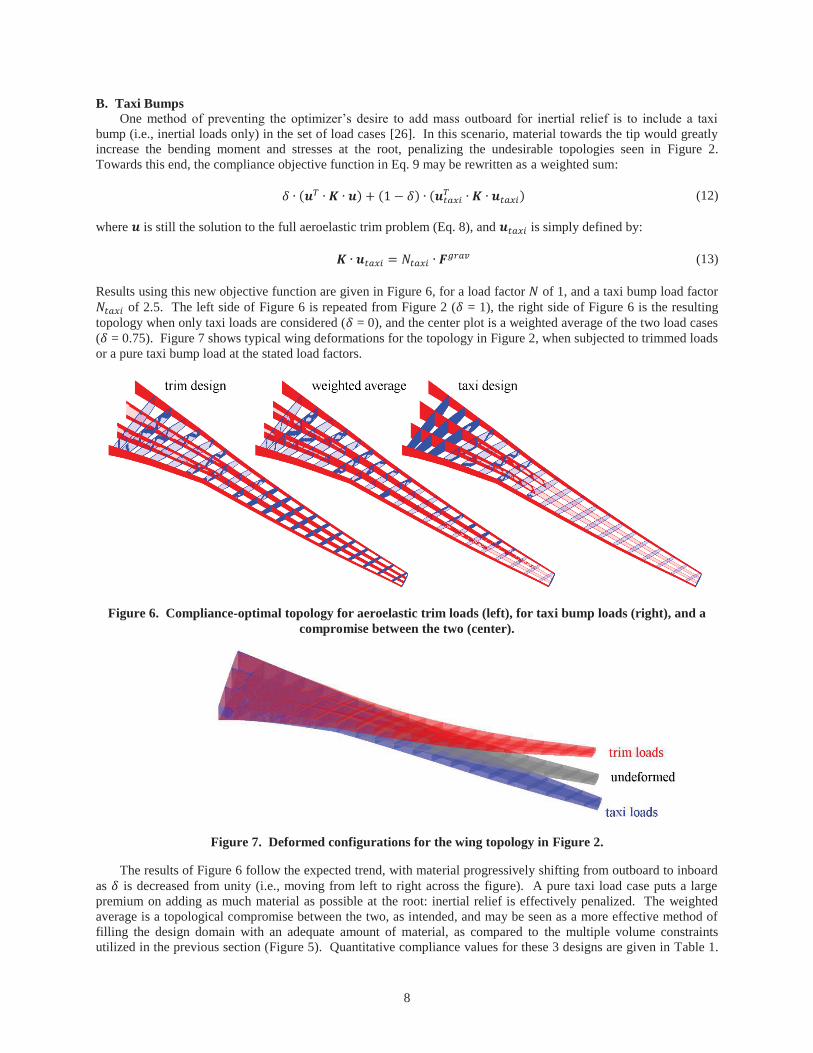
bump (i.e., inertial loads only) in the set of load cases [26]. In this scenario, material towards the tip would greatly increase the bending moment and stresses at the root, penalizing the undesirable topologies seen in Figure 2. Towards this end, the compliance objective function in Eq. 9 may be rewritten as a weighted sum:

(12)

where is still the solution to the full aeroelastic trim problem (Eq. 8), and is simply defined by: (13) Results using this new objective function are given in Figure 6, for a load factor of 1, and a taxi bump load factor

of 2.5. The left side of Figure 6 is repeated from Figure 2 ( = 1), the right side of Figure 6 is the resulting topology when only taxi loads are considered ( = 0), and the center plot is a weighted average of the two load cases ( = 0.75). Figure 7 shows typical wing deformations for the topology in Figure 2, when subjected to trimmed loads or a pure taxi bump load at the stated load factors.

Figure 6. Compliance-optimal topology for aeroelastic trim loads (left), for taxi bump loads (right), and a compromise between the two (center).

Figure 7. Deformed configurations for the wing topology in Figure 2.

The results of Figure 6 follow the expected trend, with material progressively shifting from outboard to inboard as is decreased from unity (i.e., moving from left to right across the figure). A pure taxi load case puts a large premium on adding as much material as possible at the root: inertial relief is effectively penalized. The weighted average is a topological compromise between the two, as intended, and may be seen as a more effective method of filling the design domain with an adequate amount of material, as compared to the multiple volume constraints utilized in the previous section (Figure 5). Quantitative compliance values for these 3 designs are given in Table 1.

9

The change in aeroelastic trim compliance is a far weaker function of than the taxi load compliance. This is presumably due to the fact that the aeroelastic trim problem (Eq. 8) still contains the effect of self-weight , and some topological details are influenced by these loads. This is the same reason why a value much larger than 0.5 is needed to find a suitable compromise between the two topological extremes.

Table 1. Compliance values for the topologies in Figure 6.

Trim Design 1 2.53·104 N·m 2.57·104 N·m

Compromise Design 0.75 2.58·104 N·m 1.84·104 N·m Taxi Design 0 2.85·104 N·m 1.41·104 N·m

C. Role of Aeroelasticity This section seeks to explicitly quantify the role of aeroelasticity, or fluid-structure coupling, in the compliance-

based topology optimization problem. If fluid-structure coupling is “turned off”, how would the topology change? This is of interest because 1) this assumption is typically made at early stages in the aircraft design process [8], and 2) the iterations required for the convergence of the coupled aeroelastic problem are very expensive. The role of aeroelasticity can be highlighted by specifying a fixed angle of attack , computing the flight loads a single time, and then applying these same a-priori loads to each structure during the optimization process: (14)

Aeroelastic coupling via the term in Eq. 5 is neglected, as is the trim relationship (Eq. 7) used to set , which is simply set to 2° for this exercise. The role of fluid-structure coupling can be further emphasized by neglecting the self-weight in Eq. 14, which is done here.

Results are given in Figure 8. The left side of the figure is simply repeated from Figure 3 (includes aeroelastic coupling), but the topology on the right side neglects coupling, driven by Eq. 14. Inboard, the two topologies are nearly identical, but differences are seen outboard. For the right topology without coupling, the material in both designable spars is completely removed by roughly 65% of the semispan. For the left topology with coupling, however, the cross-bracing in the leading spar extends farther towards the tip than the trailing spar. This rotates the primary stiffness axis of the wing forward, strengthening the negative bend-twist coupling (wash-out) [27]. Indeed, the design on the left of Figure 8 has a slightly lower (0.26%) than the design which neglects coupling. If this latter topology is re-analyzed with aeroelastic coupling “turned on”, it has a 4.2% worse objective function (higher compliance) than the design with coupling included.

Figure 8. Compliance-optimal topologies with (left) and without (right) aeroelastic coupling.

10

It is also of interest to note that the design on the right of Figure 8, which neglects both self-weight loads and trim requirements, is the first topology seen here which converges to its volume constraint from below, as is more typical of compliance-based topology optimization. There is no physical penalty for making this wing as heavy/stiff as possible, other than the volume constraint.

D. Aeroelastic Stresses Elastic compliance is a convenient metric for topology optimization [19], but structural design in general, and

aero-structural design in particular, is driven by the elastic stresses that develop throughout the wing box. Accounting for stresses during topology optimization is far more challenging, for a variety of reasons. First, the stresses in every finite element need to be monitored. Second, the identity of the element which contains the highest stress levels will typically change during the optimization process, leading to a discontinuity in the design space. Third, the stresses in void elements need to be handled correctly. The methods used here to resolve these issues are largely taken from Le et al. [28], and will be briefly summarized.

First, Eq. 8 is solved to compute the trim deformations on the aircraft, as above. The von Mises stresses within each finite element can then be computed in the usual manner [18]. A failure index for each element is then computed as:

(15) where is the density design variable, as above, and is the yield stress. A value greater than one indicates that the stresses in the element are too high, and the relaxation term ensures that void elements ( = 0) will be stress-free [28]. For elements that don’t coincide with design variables (the wing skins, for example), is set to unity, as these structures are always solid rather than void.

Next, the finite elements are grouped into a smaller number of patches. Each rib is divided into 3 full-depth patches, each spar is divided by rib intersections into a patch, and each skin panel is designated a patch. For the rib/spar structure in Figure 1, this leaves 273 patches. A p-norm stress measure is then used to compress all the failure indices for each element in the patch into a single value:

(16)

where is the p-norm measure (stress aggregate) for the th patch, is the number of finite elements in the th patch, is the volume of the finite element, and is the stress norm parameter. If is set to unity, is the sum of each value in the patch (weighted by the element volume). If is set to ∞, then becomes the maximum value within the patch. An intermediate value (8 is used here) will allow to change in a smooth manner in the event that the critical stresses in the patch switch from one location to another during the optimization process.

An optimization problem is then formulated to minimize all of the patch-based p-norm measures. This is done with a bound method [29]:

(17)

where the bound value is both a design variable and an objective function to be minimized, and a set of constraints (one for each patch) is enforced to keep each p-norm measure beneath this bound. Solving this optimization problem will implicitly minimize the peak stresses within the wing. Explicit control over the actual stress values ( ) is relinquished when the p-norm is used (though Ref. [28] discusses a way to reestablish the relationship between and the maximum wing stress), but stress aggregation is required so that the location of the critical stress can change within the wing, in a smooth manner amenable to gradient-based optimization.

11

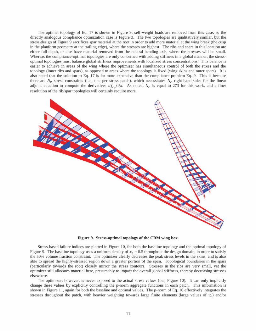
The optimal topology of Eq. 17 is shown in Figure 9: self-weight loads are removed from this case, so the directly analogous compliance optimization case is Figure 3. The two topologies are qualitatively similar, but the stress-design of Figure 9 sacrifices spar material at the root in order to add more material at the wing break (the cusp in the planform geometry at the trailing edge), where the stresses are highest. The ribs and spars in this location are either full-depth, or else have material removed from the neutral bending axis, where the stresses will be small. Whereas the compliance-optimal topologies are only concerned with adding stiffness in a global manner, the stress-optimal topologies must balance global stiffness improvements with localized stress concentrations. This balance is easier to achieve in areas of the wing where the optimizer has simultaneous control of both the stress and the topology (inner ribs and spars), as opposed to areas where the topology is fixed (wing skins and outer spars). It is also noted that the solution to Eq. 17 is far more expensive than the compliance problem Eq. 9. This is because there are stress constraints (i.e., one per stress patch), which necessitates right-hand-sides for the linear adjoint equation to compute the derivatives . As noted, is equal to 273 for this work, and a finer resolution of the rib/spar topologies will certainly require more.

Figure 9. Stress-optimal topology of the CRM wing box.

Stress-based failure indices are plotted in Figure 10, for both the baseline topology and the optimal topology of Figure 9. The baseline topology uses a uniform density of = 0.5 throughout the design domain, in order to satisfy the 50% volume fraction constraint. The optimizer clearly decreases the peak stress levels in the skins, and is also able to spread the highly-stressed region down a greater portion of the span. Topological boundaries in the spars (particularly towards the root) closely mirror the stress contours. Stresses in the ribs are very small, yet the optimizer still allocates material here, presumably to impact the overall global stiffness, thereby decreasing stresses elsewhere.

The optimizer, however, is never exposed to the actual stress values (i.e., Figure 10). It can only implicitly change these values by explicitly controlling the p-norm aggregate functions in each patch. This information is shown in Figure 11, again for both the baseline and optimal values. The p-norm of Eq. 16 effectively integrates the stresses throughout the patch, with heavier weighting towards large finite elements (large values of ) and/or

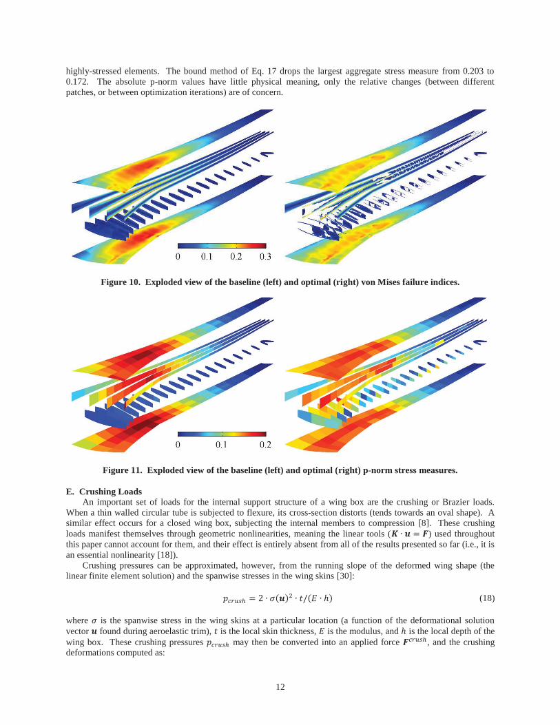
12

highly-stressed elements. The bound method of Eq. 17 drops the largest aggregate stress measure from 0.203 to 0.172. The absolute p-norm values have little physical meaning, only the relative changes (between different patches, or between optimization iterations) are of concern.

Figure 10. Exploded view of the baseline (left) and optimal (right) von Mises failure indices.

Figure 11. Exploded view of the baseline (left) and optimal (right) p-norm stress measures.

E. Crushing Loads An important set of loads for the internal support structure of a wing box are the crushing or Brazier loads.

When a thin walled circular tube is subjected to flexure, its cross-section distorts (tends towards an oval shape). A similar effect occurs for a closed wing box, subjecting the internal members to compression [8]. These crushing loads manifest themselves through geometric nonlinearities, meaning the linear tools ( ) used throughout this paper cannot account for them, and their effect is entirely absent from all of the results presented so far (i.e., it is an essential nonlinearity [18]).

Crushing pressures can be approximated, however, from the running slope of the deformed wing shape (the linear finite element solution) and the spanwise stresses in the wing skins [30]: (18) where is the spanwise stress in the wing skins at a particular location (a function of the deformational solution vector found during aeroelastic trim), is the local skin thickness, is the modulus, and is the local depth of the wing box. These crushing pressures may then be converted into an applied force , and the crushing deformations computed as:

13

(19) In summary, two finite element systems are solved at every iteration of the optimization procedure. The fully-converged aeroelastic trim deformations are first computed via Eq. 8, this solution vector is used to construct

, and then crushing deformations are computed in Eq. 19. Adjoint-based sensitivities are formulated to capture the dependence of upon .

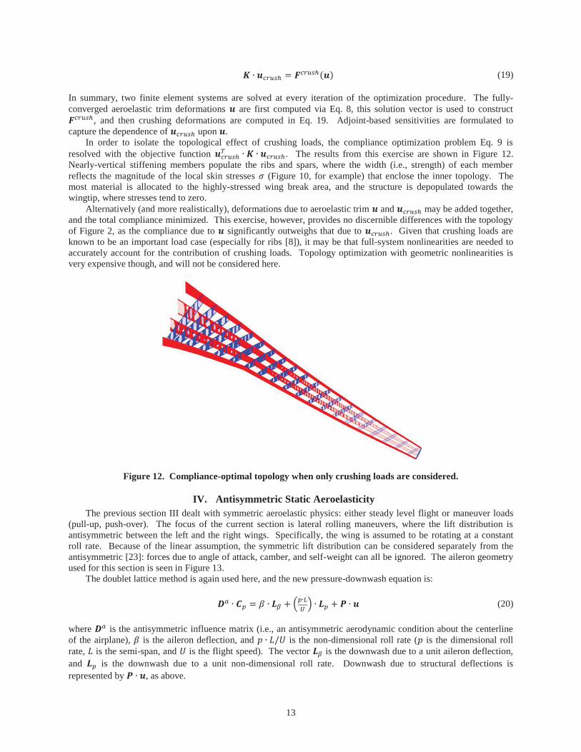
In order to isolate the topological effect of crushing loads, the compliance optimization problem Eq. 9 is resolved with the objective function . The results from this exercise are shown in Figure 12. Nearly-vertical stiffening members populate the ribs and spars, where the width (i.e., strength) of each member reflects the magnitude of the local skin stresses (Figure 10, for example) that enclose the inner topology. The most material is allocated to the highly-stressed wing break area, and the structure is depopulated towards the wingtip, where stresses tend to zero.

Alternatively (and more realistically), deformations due to aeroelastic trim and may be added together, and the total compliance minimized. This exercise, however, provides no discernible differences with the topology of Figure 2, as the compliance due to significantly outweighs that due to . Given that crushing loads are known to be an important load case (especially for ribs [8]), it may be that full-system nonlinearities are needed to accurately account for the contribution of crushing loads. Topology optimization with geometric nonlinearities is very expensive though, and will not be considered here.

Figure 12. Compliance-optimal topology when only crushing loads are considered.

IV. Antisymmetric Static Aeroelasticity The previous section III dealt with symmetric aeroelastic physics: either steady level flight or maneuver loads

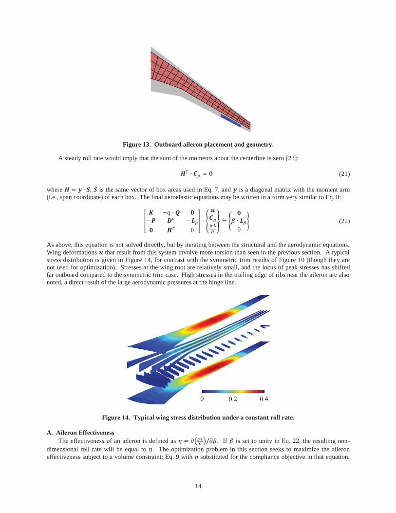
(pull-up, push-over). The focus of the current section is lateral rolling maneuvers, where the lift distribution is antisymmetric between the left and the right wings. Specifically, the wing is assumed to be rotating at a constant roll rate. Because of the linear assumption, the symmetric lift distribution can be considered separately from the antisymmetric [23]: forces due to angle of attack, camber, and self-weight can all be ignored. The aileron geometry used for this section is seen in Figure 13.

The doublet lattice method is again used here, and the new pressure-downwash equation is: (20) where is the antisymmetric influence matrix (i.e., an antisymmetric aerodynamic condition about the centerline of the airplane), is the aileron deflection, and is the non-dimensional roll rate ( is the dimensional roll rate, is the semi-span, and is the flight speed). The vector is the downwash due to a unit aileron deflection, and is the downwash due to a unit non-dimensional roll rate. Downwash due to structural deflections is represented by , as above.

14

Figure 13. Outboard aileron placement and geometry.

A steady roll rate would imply that the sum of the moments about the centerline is zero [23]: (21) where , is the same vector of box areas used in Eq. 7, and is a diagonal matrix with the moment arm (i.e., span coordinate) of each box. The final aeroelastic equations may be written in a form very similar to Eq. 8:

(22)

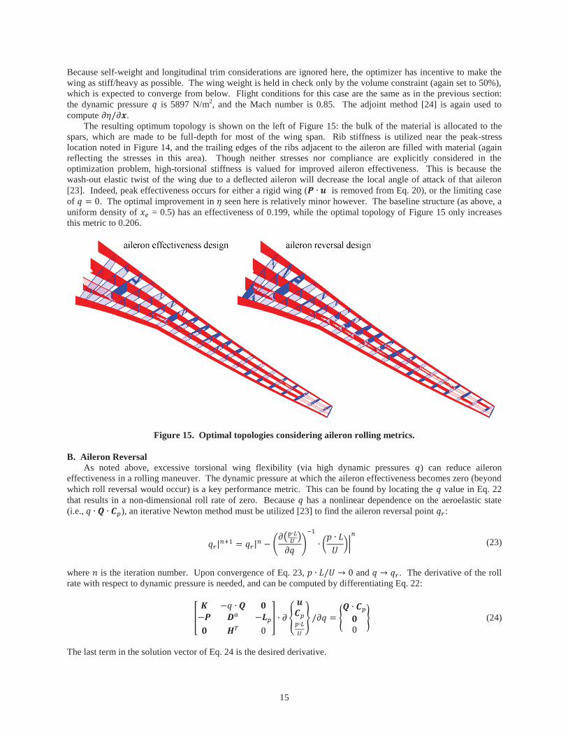
As above, this equation is not solved directly, but by iterating between the structural and the aerodynamic equations. Wing deformations that result from this system involve more torsion than seen in the previous section. A typical stress distribution is given in Figure 14, for contrast with the symmetric trim results of Figure 10 (though they are not used for optimization). Stresses at the wing root are relatively small, and the locus of peak stresses has shifted far outboard compared to the symmetric trim case. High stresses in the trailing edge of ribs near the aileron are also noted, a direct result of the large aerodynamic pressures at the hinge line.

Figure 14. Typical wing stress distribution under a constant roll rate.

A. Aileron Effectiveness The effectiveness of an aileron is defined as . If is set to unity in Eq. 22, the resulting non-

dimensional roll rate will be equal to . The optimization problem in this section seeks to maximize the aileron effectiveness subject to a volume constraint: Eq. 9 with substituted for the compliance objective in that equation.

15

Because self-weight and longitudinal trim considerations are ignored here, the optimizer has incentive to make the wing as stiff/heavy as possible. The wing weight is held in check only by the volume constraint (again set to 50%), which is expected to converge from below. Flight conditions for this case are the same as in the previous section: the dynamic pressure is 5897 N/m2, and the Mach number is 0.85. The adjoint method [24] is again used to compute .

The resulting optimum topology is shown on the left of Figure 15: the bulk of the material is allocated to the spars, which are made to be full-depth for most of the wing span. Rib stiffness is utilized near the peak-stress location noted in Figure 14, and the trailing edges of the ribs adjacent to the aileron are filled with material (again reflecting the stresses in this area). Though neither stresses nor compliance are explicitly considered in the optimization problem, high-torsional stiffness is valued for improved aileron effectiveness. This is because the wash-out elastic twist of the wing due to a deflected aileron will decrease the local angle of attack of that aileron [23]. Indeed, peak effectiveness occurs for either a rigid wing ( is removed from Eq. 20), or the limiting case of . The optimal improvement in seen here is relatively minor however. The baseline structure (as above, a uniform density of = 0.5) has an effectiveness of 0.199, while the optimal topology of Figure 15 only increases this metric to 0.206.

Figure 15. Optimal topologies considering aileron rolling metrics.

B. Aileron Reversal As noted above, excessive torsional wing flexibility (via high dynamic pressures ) can reduce aileron

effectiveness in a rolling maneuver. The dynamic pressure at which the aileron effectiveness becomes zero (beyond which roll reversal would occur) is a key performance metric. This can be found by locating the value in Eq. 22 that results in a non-dimensional roll rate of zero. Because has a nonlinear dependence on the aeroelastic state (i.e., ), an iterative Newton method must be utilized [23] to find the aileron reversal point :

(23)

where is the iteration number. Upon convergence of Eq. 23, and . The derivative of the roll rate with respect to dynamic pressure is needed, and can be computed by differentiating Eq. 22:

(24)

The last term in the solution vector of Eq. 24 is the desired derivative.

16

The topology optimization in this section maximizes under a volume constraint. The design derivatives are computed as follows. The total derivative of the roll rate with respect to topology is zero (because a

dynamic pressure will always be found in Eq. 23 to drive the roll rate to zero). The chain rule then gives:

(25)

The desired derivative is then solved as:

(26)

The derivative of the roll rate with respect to will be available from the final converged iteration of Eq. 23. The derivative of roll rate with respect to the design variables can be found from the adjoint method, as in the previous section.

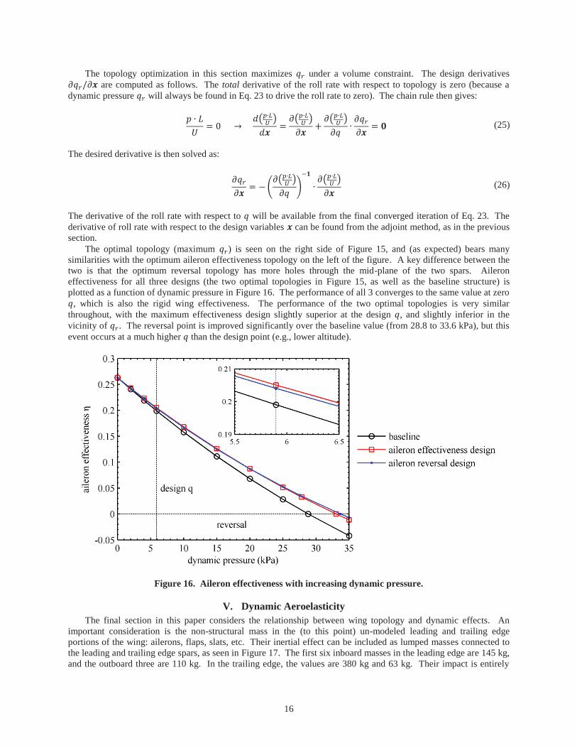
The optimal topology (maximum ) is seen on the right side of Figure 15, and (as expected) bears many similarities with the optimum aileron effectiveness topology on the left of the figure. A key difference between the two is that the optimum reversal topology has more holes through the mid-plane of the two spars. Aileron effectiveness for all three designs (the two optimal topologies in Figure 15, as well as the baseline structure) is plotted as a function of dynamic pressure in Figure 16. The performance of all 3 converges to the same value at zero

, which is also the rigid wing effectiveness. The performance of the two optimal topologies is very similar throughout, with the maximum effectiveness design slightly superior at the design , and slightly inferior in the vicinity of . The reversal point is improved significantly over the baseline value (from 28.8 to 33.6 kPa), but this event occurs at a much higher than the design point (e.g., lower altitude).

Figure 16. Aileron effectiveness with increasing dynamic pressure.

V. Dynamic Aeroelasticity The final section in this paper considers the relationship between wing topology and dynamic effects. An

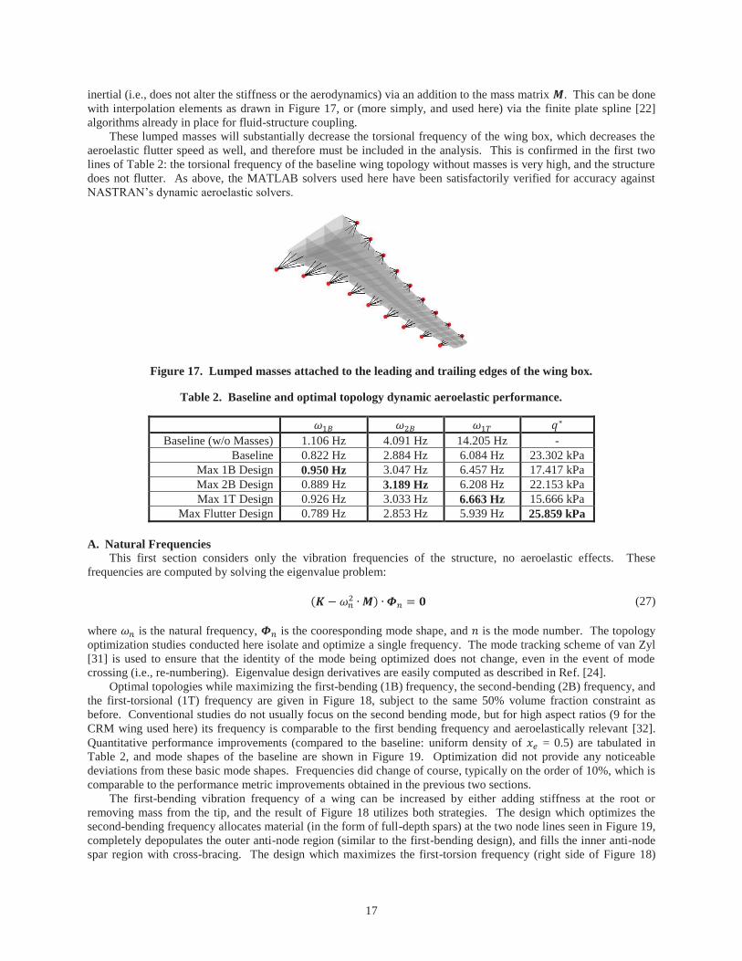
important consideration is the non-structural mass in the (to this point) un-modeled leading and trailing edge portions of the wing: ailerons, flaps, slats, etc. Their inertial effect can be included as lumped masses connected to the leading and trailing edge spars, as seen in Figure 17. The first six inboard masses in the leading edge are 145 kg, and the outboard three are 110 kg. In the trailing edge, the values are 380 kg and 63 kg. Their impact is entirely

17

inertial (i.e., does not alter the stiffness or the aerodynamics) via an addition to the mass matrix . This can be done with interpolation elements as drawn in Figure 17, or (more simply, and used here) via the finite plate spline [22] algorithms already in place for fluid-structure coupling.

These lumped masses will substantially decrease the torsional frequency of the wing box, which decreases the aeroelastic flutter speed as well, and therefore must be included in the analysis. This is confirmed in the first two lines of Table 2: the torsional frequency of the baseline wing topology without masses is very high, and the structure does not flutter. As above, the MATLAB solvers used here have been satisfactorily verified for accuracy against NASTRAN’s dynamic aeroelastic solvers.

Figure 17. Lumped masses attached to the leading and trailing edges of the wing box.

Table 2. Baseline and optimal topology dynamic aeroelastic performance.

Baseline (w/o Masses) 1.106 Hz 4.091 Hz 14.205 Hz -

Baseline 0.822 Hz 2.884 Hz 6.084 Hz 23.302 kPa Max 1B Design 0.950 Hz 3.047 Hz 6.457 Hz 17.417 kPa Max 2B Design 0.889 Hz 3.189 Hz 6.208 Hz 22.153 kPa Max 1T Design 0.926 Hz 3.033 Hz 6.663 Hz 15.666 kPa

Max Flutter Design 0.789 Hz 2.853 Hz 5.939 Hz 25.859 kPa

A. Natural Frequencies This first section considers only the vibration frequencies of the structure, no aeroelastic effects. These

frequencies are computed by solving the eigenvalue problem: (27) where is the natural frequency, is the cooresponding mode shape, and is the mode number. The topology optimization studies conducted here isolate and optimize a single frequency. The mode tracking scheme of van Zyl [31] is used to ensure that the identity of the mode being optimized does not change, even in the event of mode crossing (i.e., re-numbering). Eigenvalue design derivatives are easily computed as described in Ref. [24].

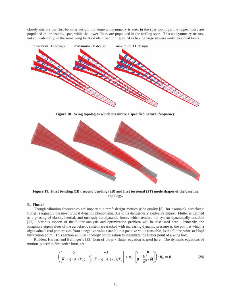
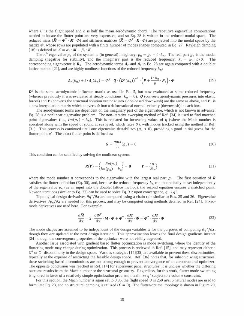
Optimal topologies while maximizing the first-bending (1B) frequency, the second-bending (2B) frequency, and the first-torsional (1T) frequency are given in Figure 18, subject to the same 50% volume fraction constraint as before. Conventional studies do not usually focus on the second bending mode, but for high aspect ratios (9 for the CRM wing used here) its frequency is comparable to the first bending frequency and aeroelastically relevant [32]. Quantitative performance improvements (compared to the baseline: uniform density of = 0.5) are tabulated in Table 2, and mode shapes of the baseline are shown in Figure 19. Optimization did not provide any noticeable deviations from these basic mode shapes. Frequencies did change of course, typically on the order of 10%, which is comparable to the performance metric improvements obtained in the previous two sections.

The first-bending vibration frequency of a wing can be increased by either adding stiffness at the root or removing mass from the tip, and the result of Figure 18 utilizes both strategies. The design which optimizes the second-bending frequency allocates material (in the form of full-depth spars) at the two node lines seen in Figure 19, completely depopulates the outer anti-node region (similar to the first-bending design), and fills the inner anti-node spar region with cross-bracing. The design which maximizes the first-torsion frequency (right side of Figure 18)

18

closely mirrors the first-bending design, but some antisymmetry is seen in the spar topology: the upper fibers are populated in the leading spar, while the lower fibers are populated in the trailing spar. This antisymmetry occurs, not coincidentally, in the same wing location identified in Figure 14 as having large stresses under torsional loads.

Figure 18. Wing topologies which maximize a specified natural frequency.

Figure 19. First bending (1B), second bending (2B) and first torsional (1T) mode shapes of the baseline topology.

B. Flutter Though vibration frequencies are important aircraft design metrics (ride-quality [8], for example), aeroelastic

flutter is arguably the most critical dynamic phenomena, due to its dangerously explosive nature. Flutter is defined as a phasing of elastic, inertial, and unsteady aerodynamic forces which renders the system dynamically unstable [23]. Various aspects of the flutter analysis and optimization problem will be discussed here. Primarily, the imaginary eigenvalues of the aeroelastic system are tracked with increasing dynamic pressure ; the point at which a eigenvalue’s real part crosses from a negative value (stable) to a positive value (unstable) is the flutter point, or Hopf bifurcation point. This section will use topology optimization to maximize the flutter point of a wing box.

Rodden, Harder, and Bellinger’s [33] form of the p-k flutter equation is used here. The dynamic equations of motion, placed in first-order form, are:

(28)

19

where is the flight speed and is half the mean aerodynamic chord. The repetitive eigenvalue computations needed to locate the flutter point are very expensive, and so Eq. 28 is written in the reduced modal space. The reduced mass ( ) and stiffness matrices ( ) are projected into the modal space by the matrix , whose rows are populated with a finite number of modes shapes computed in Eq. 27. Rayleigh damping [18] is defined as: .

The th eigenvalue of the system is (in general) imaginary: . The real part is the modal damping (negative for stability), and the imaginary part is the reduced frequency: . The corresponding eigenvector is . The aerodynamic terms and in Eq. 28 are again computed with a doublet lattice method [21], and are highly nonlinear functions of the reduced frequency : (29)

is the same aerodynamic influence matrix as used in Eq. 5, but now evaluated at some reduced frequency

(whereas previously it was evaluated at steady conditions: ). (converts aerodynamic pressures into elastic forces) and (converts the structural solution vector into slope-based downwash) are the same as above, and is a new interpolation matrix which converts into a deformational normal-velocity (downwash) in each box.

The aerodynamic terms are dependent on the imaginary part of the eigenvalue, which is not known in advance: Eq. 28 is a nonlinear eigenvalue problem. The non-iterative sweeping method of Ref. [34] is used to find matched point eigenvalues (i.e., ). This is repeated for increasing values of (where the Mach number is specified along with the speed of sound at sea level, which fixes ), with modes tracked using the method in Ref. [31]. This process is continued until one eigenvalue destabilizes ( ), providing a good initial guess for the flutter point . The exact flutter point is defined as: (30) This condition can be satisfied by solving the nonlinear system: (31)

where the mode number corresponds to the eigenvalue with the largest real part . The first equation of satisfies the flutter definition (Eq. 30), and, because the reduced frequency can theoretically be set independently of the eigenvalue (as an input into the doublet lattice method), the second equation ensures a matched point. Newton iterations (similar to Eq. 23) can be used to solve Eq. 31: upon convergence, .

Topological design derivatives are computed using a chain rule similar to Eqs. 25 and 26. Eigenvalue derivatives are needed for this process, and may be computed using methods detailed in Ref. [24]. Fixed-mode derivatives are used here. For example: (32)

The mode shapes are assumed to be independent of the design variables for the purposes of computing , though they are updated at the next design iteration. This approximation leaves the final design gradients inexact [24], though the convergence properties of the optimizer were not visibly degraded.

Another issue associated with gradient based flutter optimization is mode switching, where the identity of the fluttering mode may change during optimization. This process is reviewed in Ref. [15], and may represent either a

or discontinuity in the design space. Various strategies [14][35] are available to prevent these discontinuities, typically at the expense of restricting the feasible design space. Ref. [36] notes that, for subsonic wing structures, these switching-based discontinuities are not strong enough to prevent convergence of an aerostructural optimizer. The opposite conclusion was reached in Ref. [14] for supersonic panel structures: it is unclear whether the differing outcome results from the Mach number or the structural geometry. Regardless, for this work, flutter mode switching is ignored in favor of a relatively simple optimization problem: maximize subject to a volume constraint.

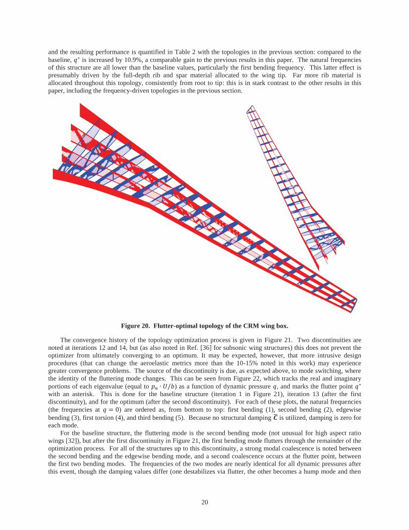
For this section, the Mach number is again set to 0.85, the flight speed is 250 m/s, 6 natural modes are used to formulate Eq. 28, and no structural damping is utilized ( ). The flutter-optimal topology is shown in Figure 20,

20

and the resulting performance is quantified in Table 2 with the topologies in the previous section: compared to the baseline, is increased by 10.9%, a comparable gain to the previous results in this paper. The natural frequencies of this structure are all lower than the baseline values, particularly the first bending frequency. This latter effect is presumably driven by the full-depth rib and spar material allocated to the wing tip. Far more rib material is allocated throughout this topology, consistently from root to tip: this is in stark contrast to the other results in this paper, including the frequency-driven topologies in the previous section.

Figure 20. Flutter-optimal topology of the CRM wing box.

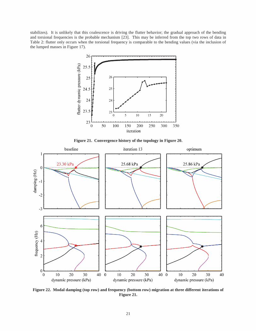
The convergence history of the topology optimization process is given in Figure 21. Two discontinuities are noted at iterations 12 and 14, but (as also noted in Ref. [36] for subsonic wing structures) this does not prevent the optimizer from ultimately converging to an optimum. It may be expected, however, that more intrusive design procedures (that can change the aeroelastic metrics more than the 10-15% noted in this work) may experience greater convergence problems. The source of the discontinuity is due, as expected above, to mode switching, where the identity of the fluttering mode changes. This can be seen from Figure 22, which tracks the real and imaginary portions of each eigenvalue (equal to ) as a function of dynamic pressure , and marks the flutter point with an asterisk. This is done for the baseline structure (iteration 1 in Figure 21), iteration 13 (after the first discontinuity), and for the optimum (after the second discontinuity). For each of these plots, the natural frequencies (the frequencies at ) are ordered as, from bottom to top: first bending (1), second bending (2), edgewise bending (3), first torsion (4), and third bending (5). Because no structural damping is utilized, damping is zero for each mode.

For the baseline structure, the fluttering mode is the second bending mode (not unusual for high aspect ratio wings [32]), but after the first discontinuity in Figure 21, the first bending mode flutters through the remainder of the optimization process. For all of the structures up to this discontinuity, a strong modal coalescence is noted between the second bending and the edgewise bending mode, and a second coalescence occurs at the flutter point, between the first two bending modes. The frequencies of the two modes are nearly identical for all dynamic pressures after this event, though the damping values differ (one destabilizes via flutter, the other becomes a hump mode and then

21

stabilizes). It is unlikely that this coalescence is driving the flutter behavior; the gradual approach of the bending and torsional frequencies is the probable mechanism [23]. This may be inferred from the top two rows of data in Table 2: flutter only occurs when the torsional frequency is comparable to the bending values (via the inclusion of the lumped masses in Figure 17).

Figure 21. Convergence history of the topology in Figure 20.

Figure 22. Modal damping (top row) and frequency (bottom row) migration at three different iterations of Figure 21.

22

For all of the designs in Figure 22, the torsional mode begins to destabilize as well. For the optimal design, this mode actually flutters, but this second flutter point occurs well above the first. A final interesting point concerning these figures is the advent of a series of aerodynamic lag roots [34] at a dynamic pressure slightly before . One oscillatory root and two non-oscillatory roots (only one of which can be seen in the figure) appear. In the baseline topology, the oscillatory root collides with the edgewise bending root, annihilating them both. For the optimal design, the second bending mode disappears. It may be recalled that, when the optimization began (for the baseline structure), the second bending mode was the fluttering mode. When the optimization is complete, this same mode no longer exists at higher dynamic pressures.

VI. Conclusions Aeroelastic topology optimization has been conducted within a wing box for the Common Research Model, a

high aspect ratio subsonic transport wing. The outer mold line is populated with a fixed lattice of orthogonal ribs and spars, and then gradient-based topology optimization is conducted within each of these shell structures. This parameterization allows for the development of lightening holes, the reduction of full-depth members to truss- or cross-braced support structures, or the complete removal of the interior of a given member, leaving behind a cap or stringer structure.

Many different rib and spar topologies have been developed in this paper, each highlighting the best way to improve a single aeroelastic metric of interest under a prescribed amount of material within the design domain (i.e., a constant wing mass). This approach can uncover the relationship between topology and aeroelastic physics, identify which metrics are more or less affected by changes in topology, and therefore provide a deeper understanding of the design which is ultimately obtained when all metrics are considered simultaneously (i.e., minimize one with constraints on the others) during a unified aircraft design process.

The results in this paper are divided into three sections. For symmetric static aeroelasticity (section III), minimum-compliance designs (under a volume constraint) are found for trimmed flight loads, a taxi bump load, and a weighted sum of the two. Further results detail the topological effect of the pull-up load factor, the self-weight loading, the aeroelastic coupling terms, the inclusion of stress metrics, and crushing Brazier loads. Antisymmetric static aeroelasticity (section IV) results assume a pure rolling maneuver at a constant rate. Topologies are shown which maximize either the aileron effectiveness, or the aileron-reversal dynamic pressure. Dynamic effects are considered in section V, with topologies which optimize a given natural frequency (first bending, second bending, or torsional modes), or optimize the flutter point of the wing, computed with the unsteady p-k method.

A comprehensive aircraft design will, of course, utilize only one wing topology. It is unlikely that any of the topologies shown here will represent this final design, for a number of reasons. First, a wing structure must be designed under multiple metrics simultaneously, rather than one at a time, as done here. Secondly, even though many different types of aeroelastic metrics have been considered, important factors are still un-modeled (panel buckling, drag, fuel burn, etc.). Third, additional geometric details (and their associated loads) have been omitted in this conceptual design exercise: fuel loads, engine loads, landing gear loads, etc. These structures will undoubtedly impact the structural design, and need to be included. Finally, and as noted above, the internal topology optimization used here should be done in conjunction with additional tailoring tools (focused on the wing skins, for example).

Regardless, the work conducted here has demonstrated the feasibility of developing, in an automated manner, detailed structural topologies within the ribs and spars of a wing box, driven by complex aeroelastic physics. Future tasks will work to account for the additional design scenarios listed above.

Acknowledgements This work is funded by the Fixed Wing project under NASA’s Fundamental Aeronautics Program.

References [1] Wang, W., Guo, S., Yang, W., “Simultaneous Partial Topology and Size Optimization of a Wing Structure Using Any

Colony and Gradient Based Methods,” Engineering Optimization, Vol. 43, No. 4, pp. 433-446, 2011. [2] Balabanov, V., Haftka, R., “Topology Optimization of Transport Wing Internal Structure,” Journal of Aircraft, Vol. 33, No.

1, 1996, pp. 232-233. [3] Locatelli, D., Mulani, S., Kapania, R., “Wing-Box Weight Optimization Using Curvilinear Spars and Ribs (SpaRibs),”

Journal of Aircraft, Vol. 48, No. 5, pp. 1671-1684, 2011. [4] Kobayashi, M., Pedro, H., Kolonay, R., Reich, G., “On a Cellular Division Method for Aircraft Structural Design,”

Aeronautical Journal, Vol. 113, No. 1150, pp. 821-831, 2009.

23

[5] Kim, W., Grandhi, R., Haney, M., “Multiobjective Evolutionary Structural Optimization Using Combined Static/Dynamic Control Parameters,” AIAA Journal, Vol. 44, No. 4, pp. 794-802, 2006.

[6] James, K., Martins, J., “An Isoparametric Approach to Level Set Topology Optimization Using a Body-Fitted Finite Element Mesh,” Computers and Structures, vol. 90, pp. 97-106, 2012.

[7] Dunning, P., Brampton, C., Kim, H., “Multidisciplinary Level Set Topology Optimization of the Internal Structure of an Aircraft Wing,” World Congress on Structural and Multidisciplinary Optimization, Orlando FL, May 19-24, 2013.

[8] Niu, M., Airframe Structural Design, Conmilit Press Ltd., Hong Kong, 1988. [9] Maute, K., Allen, M., “Conceptual Design of Aeroelastic Structures by Topology Optimization,” Structural and

Multidisciplinary Optimization, Vol. 27, No. 1, pp. 27-42, 2004. [10] Eschenauer, H., Olhoff, N. “Topology Optimization of Continuum Structures: A Review,” Applied Mechanics Reviews, Vol.

54, pp. 331-390, 2001. [11] Krog, L., Tucker, A., Kemp, M., Boyd, R., “Topology Optimization of Aircraft Wing Box Ribs,” AIAA Multidisciplonary

Analysis and Optimization Conference, Albany NY, August 30 – September 1, 2004. [12] Maute, K., Reich, G., “Integrated Multidisciplinary Topology Optimization Approach to Adaptive Wing Design,” Journal of

Aircraft, Vol. 43, No. 1, pp. 253-263, 2006. [13] Oktay, E., Akay, H., Merttopcuoglu, O., “Parallelized Structural Topology Optimization and CFD Coupling for Design of

Aircraft Wing Structures,” Computers and Fluids, Vol. 49, pp. 141-145, 2011. [14] Stanford, B., Beran, P., “Aerothermoelastic Topology Optimization with Flutter and Buckling Metrics,” Structural and

Multidisciplinary Optimization, Vol. 48, No. 1, pp. 149-171, 2013. [15] Stanford B., Beran, P., Bhatia, M., “Aeroelastic Topology Optimization of Blade-Stiffened Panels,” Journal of Aircraft,

accepted for publication, 2013. [16] Dillinger, J., Klimmek, T., Abdalla, M., Gürdal, Z., “Stiffness Optimization of Composite Wings with Aeroelastic

Constraints,” Journal of Aircraft, Vol. 50, No. 4, pp. 1159-1168, 2013. [17] Vassberg, J., DeHaan, M., Rivers, S., Wahls, R., “Development of a Common Research Model for Applied CFD Validation

Studies,” AIAA Applied Aerodynamics Conference, Honolulu, Hawaii, August 10-13, 2008. [18] Cook, R., Malkus, D., Plesha, M., Witt, R., Concepts and Applications of Finite Element Analysis, Wiley, New York, 2002. [19] Bendsøe, M., Sigmund, O., Topology Optimization, Springer, Berlin, Germany, 2003. [20] Bruyneel, M., Duysinx, P., “Note on Topology Optimization of Continuum Structures Including Self-Weight,” Structural

and Multidiscisplinary Optimization, Vol. 29, No. 4, pp. 245-256, 2005. [21] Rodden, W., Taylor, P., McIntosh, S., “Further Refinement of the Subsonic Doublet-Lattice Method,” Journal of Aircraft,

Vol. 35, No. 5, pp. 720-727, 1998. [22] Appa, K., “Finite-Surface Spline,” Journal of Aircraft, Vol. 26, No. 5, pp. 495-496, 1989. [23] Bisplinghoff, R., Ashley, H., Halfman, R., Aeroelasticity, Addison-Wesley, Cambridge, MA, 1955. [24] Haftka, R., Gürdal, Z., Elements of Structural Optimization, Kluwer Academic Publishers, Dordecht, The Netherlands,

1992. [25] Svanberg, K., “The Method of Moving Asymptotes – a New Method for Structural Optimization,” International Journal for

Numerical Methods in Engineering, Vol. 24, No. 2, pp. 359-373, 1987. [26] Wakayama, S., Kroo, I., “Subsonic Wing Planform Design Using Multidisciplinary Optimization,” Journal of Aircraft, Vol.

32, No. 4, pp. 746-753, 1995. [27] Shirk, M., Hertz, T., Weisshaar, T., “Aeroelastic Tailoring – Theory, Practice, and Promise,” Journal of Aircraft, Vol. 23,

No. 1, pp. 6-18, 1986. [28] Le, C., Norato, J., Bruns, T., Ha, C., Tortorelli, D., “Stress-Based Topology Optimization for Continua,” Structural and

Multidisciplinary Optimization, Vol. 41, No. 4, pp. 605-620, 2010. [29] Seyranian, A., Lund, E., Olhoff, N., “Multiple Eigenvalues in Structural Optimization Problems,” Structural Optimization,

Vol. 8, No. 4, pp. 207-227, 1994. [30] Jensen, F., Weaver, P., Cecchini, L., Stang, H., Nielsen, R., “The Brazier Effect in Wind Turbine Blades and its Influence on

Design,” Wind Energy, Vol. 15, No. 2, pp. 319-333, 2012. [31] van Zyl, L., “Use of Eigenvectors in the Solution of the Flutter Equation,” Journal of Aircraft, Vol. 30, No. 4, pp. 553-554,

1993. [32] Tang, D., Dowell, E., “Experimental and Theoretical Study on Aeroelastic Response of High-Aspect Ratio Wings,” AIAA

Journal, Vol. 39, No. 8, pp. 1430-1441, 2001. [33] Rodden, W., Harder, R., Bellinger, E., “Aeroelastic Addition to NASTRAN,” NASA CR 3094, 1979. [34] van Zyl, L., “Aeroelastic Divergence and Aerodynamic Lag Roots,” Journal of Aircraft, Vol. 38, No. 3, pp. 586-588, 2001. [35] Haftka, R., “Parametric Constraints with Application to Optimization for Flutter Using a Continuous Flutter Constraint,”

AIAA Journal, Vol. 13, pp. 471-475, 1975. [36] Stanford, B., Beran, P., “Optimal Structural Topology of a Platelike Wing for Subsonic Aeroelastic Stability,” Journal of

Aircraft, Vol. 48, No. 4, pp. 1193-1203, 2011.