Embed Size (px)
Citation preview

Optimal Taxation and Cross-Price Effects on Labor Supply:Estimates of the Optimal Gas Tax
Sarah E. WestMacalester College
Roberton C. Williams IIIUniversity of Texas at Austin and NBER
March 2005
Key Words: optimal taxation, gasoline, labor supply, second-best environmental taxes, demandsystem
JEL Classification Nos.: H21, H23, Q5
For their helpful comments and suggestions, we thank Don Fullerton, Eban Goodstein, LarryGoulder, Michael Greenstone, Dan Hamermesh, Shulamit Kahn, Gib Metcalf, Ian Parry,Raymond Robertson, Dan Slesnick, Steve Trejo, Pete Wilcoxen, Frank Wolak, Ann Wolverton,and seminar participants at the Brookings Institution, the NBER Environmental EconomicsWorking Group, the Universities of California (Berkeley and Santa Barbara), Maryland,Minnesota, Texas, and Virginia, Syracuse University, the Southern Economics Association, andthe U.S. Environmental Protection Agency. For their excellent research assistance, we thankChris Lyddy, Trey Miller, and Jim Sallee. Williams is grateful for financial support from theAndrew W. Mellon Fellowship in Economic Studies at the Brookings Institution and from theWilliam and Flora Hewlett Foundation.

Optimal Taxation and Cross-Price Effects on Labor Supply:New Estimates of the Optimal Gas Tax
This study estimates parameters necessary to calculate the optimal second-best gasoline
tax, most notably the cross-price elasticity between gasoline and leisure. Prior theoretical work
indicates the importance of this elasticity, but despite this, almost none of the prior studies of
commodity taxation (and none of the studies on second-best environmental regulation) actually
estimate it. Using household data, we find that gasoline is a relative complement to leisure, and
thus that the optimal gasoline tax is significantly higher than marginal damages–the opposite of
the result suggested by the prior literature. Indeed, even if there were no externalities at all
associated with gasoline, the optimal tax rate would still be almost equal to the average gas tax
rate in the U.S. Following this approach to estimate cross-price elasticities with leisure could
strongly influence estimates of optimal rates for other important commodity or pollution taxes.
Sarah E. West Roberton C. Williams IIIDepartment of Economics Department of EconomicsMacalester College University of Texas at Austin1600 Grand Ave. Austin, TX 78712St. Paul, MN 55105 and [email protected] [email protected]

1
As first shown by Corlett and Hague (1953), optimal commodity tax rates depend
crucially on the cross-price elasticity with leisure. Leisure cannot be taxed, and thus individuals
consume more than the efficient amount of it. However, government can implicitly tax leisure by
raising taxes on goods that are more complementary to leisure than is the average good and
lowering taxes on goods that are more substitutable for leisure. Subsequent theoretical work
extends this basic insight to more complex models of taxation. But despite the theoretical
importance of this elasticity, almost none of the empirical studies of commodity taxation
estimate it: nearly all assume that leisure is separable from other goods in utility, and many even
assume that labor supply is fixed.
In this paper, we focus on the gas tax, which is one of the most important practical
examples of a differentiated commodity tax: in the U.S., it raises more revenue than any other
commodity tax at both state and federal levels, and it accounts for an even larger share of revenue
in other developed nations. It also plays an important role as a corrective tax, since gasoline use
entails many negative externalities, including pollution, traffic congestion, and vehicle accidents.
We estimate the cross-price elasticity between gasoline and leisure, along with other
important parameters, and calculate the optimal gas tax based on these estimates. We use
household-level data from the 1996-1998 Consumer Expenditure Surveys, merged with price data
from the American Chambers of Commerce Researchers’ Association (ACCRA) cost of living
index and tax data from the National Bureau of Economic Research (NBER) TAXSIM model.
We employ Deaton and Muellbauer’s (1980) Almost Ideal Demand System (AIDS), which does
not impose separability, unlike most other widely used demand systems.
We find that gasoline is a leisure complement, and thus that the optimal gas tax exceeds
the marginal external damage associated with gas use by roughly 35%. Even if gasoline use
entailed no negative externalities at all, the optimal gas tax would still almost equal the average
rate in our sample. One possible explanation for this complementarity is that driving is a
relatively time-intensive good, and time-intensive goods tend to be leisure complements, as
suggested by Becker (1965). Another possible explanation is that the demand for leisure driving
is much more elastic than is the demand for commuting.

2
These results clearly illustrate the practical importance of estimating the cross-price
elasticity with leisure when calculating optimal tax rates–something no prior study has done. To
our knowledge, Madden (1995) is the only previous empirical study on commodity taxes that
focuses on the cross-price elasticity with leisure.1 Contrary to our results, it concludes that this
elasticity is relatively unimportant. Diewert and Lawrence (1996) also estimate this elasticity,
but do not specifically focus on it, so its influence on their results is unclear.2 Both studies rely
on aggregate time-series data sets, which are limited by small sample sizes and highly collinear
prices. Moreover, estimates based on such data are subject to aggregation bias.3 Because we use
household-level data, we can employ a more flexible functional form for demand, and our
estimates should be much more precise. The latter advantage is difficult to confirm, however,
because ours is the first study to report confidence intervals for its optimal tax estimates.
Because of gasoline’s role as a corrective tax, this paper also makes an important
contribution to the recent literature on second-best optimal environmental regulation. Theoretical
work in this area has shown that the optimal pollution tax depends on the cross-price elasticity
between polluting goods and leisure, for exactly the same reason that optimal commodity taxes
do.4 But empirical papers have not previously estimated this elasticity. We provide the first
estimate of the cross-price elasticity between a polluting good and leisure, and examine its
implications for environmental taxation. Prior work in this literature suggests that the optimal tax
on a polluting good will typically be less than marginal pollution damage. In contrast, as noted
above, we find that the optimal gas tax substantially exceeds marginal damage.
Thus, for both literatures–on optimal commodity taxes and on optimal environmental
regulation–this study demonstrates the need to explicitly estimate cross-price elasticities with
1 A number of studies have focused on the effects of allowing nonseparability among consumption goods (e.g.,Ray, 1986, or Decoster and Schokkaert, 1990), and nearly all recent studies on commodity taxation allow this sortof nonseparability. But these studies still assume that leisure is separable or that labor supply is fixed.2 Each of these studies considers only the effects of marginal tax reforms, and does not report optimal taxes, so theirresults are not strictly comparable to ours. But the two concepts are closely related, and both depend in the sameway on the cross-price elasticity with leisure.3 Blundell et al. (1993) studies this problem, and concludes that “aggregate data alone are unlikely to producereliable estimates of structural price and income coefficients.” (p. 570).4 For example, see Bovenberg and De Mooij (1994). Kim (2002) focuses specifically on this issue.

3
leisure, rather than simply making assumptions such as separability that pin down that elasticity.
And recent theoretical work shows that the cross-price elasticity with leisure influences optimal
policy in many contexts other than taxation and environmental policy.5 Our results suggest that
it could be important to estimate this elasticity in those other contexts as well.
The next section of this paper develops a simple theoretical model and derives an
expression for the optimal commodity tax on a good with an associated externality. Subsequent
sections describe the empirical model, data, estimation results, and the implied optimal tax rate.
The final section presents conclusions and suggests directions for future research.
I. A Theoretical Model
This section presents a simple theoretical model and uses it to derive an expression for
the optimal tax on a good with an associated negative externality. This model resembles those
used in recent studies of second-best optimal environmental taxes, but differs in two respects: it
does not assume that leisure is separable, that the utility function is homothetic, or that the
polluting good is an average substitute for leisure; and it allows for multiple households (and
multiple individuals in a household), rather than assuming a representative agent.6
The model is also very similar in structure to most models used in the optimal commodity
tax literature. But it differs in that it incorporates an externality, includes only two produced
goods, and ignores distributional considerations. We include the externality because the gas tax is
an important corrective tax as well as a commodity tax. It would be simple to extend our model
to allow more goods or to consider distribution, but since our primary focus is on the influence of
the cross-price elasticity with leisure, we keep the rest of the model as simple as possible.
Each household in the economy consumes a dirty (i.e., polluting) good (D), a clean good
(C), and a government-provided public good (G). The utility function for household h is
5 See, for example, Browning (1997) on the welfare cost of monopoly, Goulder and Williams (2003) on the excessburden of taxation, Parry (1999) on agricultural policy, or Williams (1999) on trade policy.6 We allow multiple households not because of distributional considerations, but simply because the aggregatedemands in our empirical model do not equal the demand of a representative household (as is briefly discussed inthe next section). Recent papers that use models similar to ours include Goulder et al. (1999) and Parry et al.(1999). Both assume a representative agent and assume that the polluting good is an average substitute for leisurein order to calculate optimal tax rates.

4
(1) Uh lh ,Ch,Dh,G( ) − φh D( ) ,
where U is continuous and quasi-concave and the function
�
φ h represents the disutility from an
externality associated with the economy-wide total consumption of the dirty good.7 The
elements
�
lhi of the vector
�
lh represent hours of leisure for each of the adults in the household.
The time constraint for individual i is
(2)
�
L = Lhi + lhi,
where L is the time endowment and
�
Lhi is hours worked. The household budget constraint is
(3)
�
pChCh + pD
h Dh =Y h ≡ Ih + whiLhii∑ ,
where w is the after-tax wage, I is after-tax non-labor income, and
�
Y h is total after-tax income,
which equals total expenditure. The consumer price of the dirty good ( pD ) is given by
(4) pDh = p D
h + τD ,
where p D is the producer price and τD is a unit tax on the dirty good. The clean good is untaxed,
and thus its producer price (
�
p C ) and consumer price (
�
pC ) are equal.8 The after-tax wage is
(5)
�
whi = w hi − τ Lhi,
where w is the pre-tax wage and
�
τ L is the marginal tax per unit of labor. After-tax non-labor
income is given by
(6)
�
Ih = I h −T h ,
where
�
I is pre-tax non-labor income and T is a lump-sum tax or transfer.9
Each of the three goods is produced under perfect competition with constant returns to
scale. We assume that non-labor income is derived from ownership of a fixed factor that is a
perfect substitute for labor.10 These assumptions imply that the pre-tax wage and all producer
7 For simplicity, we assume that the damage from the externality appears only as a separable term in utility. Ifdamages were to enter in some other form, that could also affect labor supply and thus influence the optimal taxrate. See Bovenberg and van der Ploeg (1994) and Williams (2002 and 2003) for further discussion on this point.8 This assumption entails no loss of generality, because any tax system that taxes the clean good can berenormalized as a system with a higher income tax and no clean good tax.9 Note that
�
τ L and T could represent a linear tax system or a (household-specific) local linear approximation to anonlinear tax system.10 This is unrealistic, but provides a simple way to model non-labor income. For a similar model in which thefixed factor isn’t a perfect substitute for labor, see Williams (2002). The model in Bovenberg and Goulder (1996)has non-labor income derived from capital, but is far more complex and thus cannot be solved analytically.

5
prices are exogenously fixed and that the aggregate production constraint is
(7)
�
I h + w hiLhi
i∑
⎛
⎝ ⎜
⎞
⎠ ⎟
h∑ = p GG + p C
hCh + p Dh Dh[ ]
h∑ ,
where p G is the producer price of the public good. The government’s budget constraint is
(8)
�
τDh Dh + τ L
hiLhi
i∑ + T h
⎡
⎣ ⎢
⎤
⎦ ⎥
h∑ = p GG .
The level of the public good is assumed to be fixed, with any change in revenue from the dirty
good tax offset by adjusting
�
τ L and T, following
(9)
�
τ Lhi = ˆ τ L
hi + τY w hi − ˆ τ Lhi( ) and
�
Τh = ˆ T h + τY I h − ˆ T h( ) ,
where
�
ˆ τ Lhi and
�
ˆ T h are constant, and
�
τY adjusts to hold government revenue constant as τD varies.
Equation (9) implies that the reduction in household h’s taxes from a decrease in
�
τY will be
proportional to
�
Y h . This could represent adjusting a broad-based consumption tax, renormalized
as an income tax, or could represent an income tax cut that is proportional to after-tax income.11
Each household maximizes utility (1) subject to its time constraint (2) and budget
constraint (3), taking as given prices, tax rates, the level of the public good, and the level of
pollution. This yields the first-order conditions
(10)
�
∂Uh ∂Ch = pChλh ;
�
∂Uh ∂Dh = pDh λh ;
�
∂Uh ∂lhi = whiλh ,
where λh is the marginal utility of after-tax income. Together with the constraints given
previously, these implicitly define the (uncompensated) demand functions
(11)
�
Ch pCh , pD
h ,wh,Ih( ) ;
�
Dh pCh , pD
h ,wh,Ih( );
�
lhi pCh , pD
h ,wh,Ih( ) .
To derive an expression for the aggregate change in utility from a change in the tax on the
dirty good, we take the total derivative of utility (1) with respect to τD , sum over households,
substitute in the first-order conditions (10), subtract the total derivatives with respect to τD of
the time constraint (2) and aggregate production constraint (7), and rearrange terms. This gives
11 We choose this approach for adjusting the income tax because it implies that raising the dirty good tax andlowering the income tax will not shift the tax burden from labor to non-labor income or vice-versa. In this model, atax on non-labor income is nondistortionary, because we represent non-labor income as lump-sum. But in the realworld, taxes on non-labor income are distortionary, and thus we do not want the model’s results to be driven by theeffect of shifting the tax burden onto or off of non-labor income. The results would be similar if the added revenuewere used to purchase more of the public good, as long as the level of the public good is close to the optimum.

6
(12)1λh
dUh
dτDh∑ = τD −θ( ) dD
h
dτD− τ L
hi dlhi
dτDi∑⎡
⎣⎢
⎤
⎦⎥
h∑ ,
where θ is the marginal external damage (MED) per unit of D, measured in money units:
(13) θ =1λh
∂φ h
∂Dh∑ .
Expression (12) equals the change in deadweight loss in the two distorted markets: the
distortion in the dirty good market τD −θ( ) times the change in dirty good consumption, plus
the distortion in the labor market
�
τ L( ) times the change in labor supply. This is a pure efficiency
measure; as previously noted, we do not consider distributional issues in this paper.
The total derivatives in (12) include not only the effect of the increase in the dirty good
tax, but also the effect of the resulting income tax cut. This makes little difference for the dirty
good, where the effect of the income tax change will be tiny relative to the effect of the dirty good
tax, but will be much more important for labor supply. Thus, it is useful to rewrite the term for
the labor market in (12) in terms of
�
∂l ∂pD rather than
�
dl dpD . To do this, we first define η ,
which is the marginal cost of public funds (MCPF). As shown in Appendix 1, η is given by
(14)
�
η = Y h
h∑ Y h + τ L
hi ∂lhi
∂IhIh + ∂lhi
∂whj whj
j∑
⎛
⎝ ⎜ ⎜
⎞
⎠ ⎟ ⎟
i∑
⎡
⎣ ⎢ ⎢
⎤
⎦ ⎥ ⎥ h
∑ .
This is the marginal cost to households of raising government revenue via the income tax; thus, it
is the ratio of the loss to households to the revenue raised for a marginal increase in this tax.12
We can then find the optimal tax rate by setting the rewritten version of (12) (see
Appendix 1 for this expression) equal to zero and solving for τD* . This gives
(15) τD* =
θη+ τ L
hi ∂lhi
∂ pDh − η −1
ηDh
i∑⎡⎣⎢
⎤
⎦⎥
h∑ dDh
dτDh∑ .
The first term in this expression is the externality-correcting portion of the optimal tax,
12 This definition of the MCPF considers only effects in the labor market; it omits the effects of changes inenvironmental quality and changes in revenue from the environmental tax resulting from a change in the income tax.This expression for the MCPF and those typically used in the prior literature differ slightly because of differences inmodel assumptions. They are equivalent for the special case of this model that matches the typical assumptions inthe prior literature: only one household, only one individual in that household, and no non-labor income.

7
equal to marginal damage divided by the MCPF. In an otherwise undistorted economy, this term
would simply equal marginal damage; this rate would fully correct the externality. But in a
second-best economy, the optimal tax rate represents a compromise between the rate that would
fully correct the externality and the rate that raises revenue most efficiently. Thus, the more
important government revenue is (i.e., the higher the MCPF), the smaller this term will be.
The second term is the tax rate that would be optimal if there were no externality, which
depends on the cross-price elasticity between the dirty good and leisure. When the dirty good is
a stronger substitute for leisure than is the average good, this term is negative and thus decreases
the optimal tax on the polluting good. If the dirty good is a weaker-than-average leisure
substitute or a complement to leisure, this term is positive and thus increases the optimal tax.
Many papers on commodity tax reforms assume that labor supply is fixed (see Ahmad
and Stern, 1984, and the subsequent work that it inspired). This is also the implicit assumption
in first-best studies of environmental policy. It would imply that the optimal tax in the absence
of any externality–the second term in (15)–equals zero and that η =1. Thus, the optimal tax
simply equals the marginal damage from the externality (θ ). In this case, raising revenue entails
no distortion, so the optimal tax is just the level that fully corrects the externality.
The recent literature on second-best optimal environmental taxes allows labor supply to
vary, but typically assumes that utility is homothetic and that leisure is separable–or,
equivalently, that the polluting good is an average substitute for leisure. In this case, even though
the cross-price elasticity with leisure is not zero, there is no need to estimate it, because it is a
simple function of the own-price labor supply elasticity. Just as in the case of fixed labor
supply, this implies that the optimal tax in the absence of an externality equals zero, but does not
restrict η . Therefore the optimal tax in this case is θ η .
Finally, some studies assume that leisure is separable in utility, but do not impose
homotheticity.13 This is the weakest of the assumptions commonly used in prior work, but is
still very restrictive: prior estimates of the joint demand for goods and leisure decisively reject
13 This is a common set of assumptions in the optimal commodity tax literature, starting with Atkinson andStiglitz (1972). Studies of environmental taxation that make this assumption include Jorgenson and Wilcoxen(1993), Parry and Small (2005), and Ballard et al. (2005).

8
separability.14 But it is still commonly used, because it allows the calculation of optimal taxes
without including labor supply in the estimation at all, and because of the perception (due at least
in part to Madden, 1995) that imposing separability has little or no practical effect on the results
of studies of commodity taxation. Imposing separability allows the derivative of leisure demand
with respect to the price of the dirty good to be expressed as
(16)
�
∂lhi
∂pDh = −Dh ∂lhi
∂Ih+ εDX
h whj
Y h∂lhi
∂whj −∂lhi
∂IhLhj
⎛
⎝ ⎜
⎞
⎠ ⎟
j∑
⎡
⎣ ⎢ ⎢
⎤
⎦ ⎥ ⎥ ,
where εDX is the expenditure elasticity of demand for gasoline. This implies that a luxury must
be a relative substitute for leisure, while a necessity must be a relative complement to leisure.
II. An Empirical Model
The optimal tax rate in (15) depends on several own-price and cross-price derivatives of
demand. In this section, we first specify the demand system that we use to estimate these
derivatives. Then we describe the data, variable derivation, and summary statistics. Finally, we
discuss the estimation technique and system estimation results.
A. Specification of the Demand System
We use the Almost Ideal Demand System (AIDS), as derived in Deaton and Muellbauer
(1980). The system is defined over gasoline (the dirty good), leisure, and a composite of all other
goods (the clean good). The AIDS provides a first-order approximation to any demand system,
satisfies the axioms of choice, and does not assume separability or homotheticity.
In their budget share form, the AIDS demand equations for household h are
(17)
�
s jh = α j
h + γ jk log pkh + β j log y
h Ph( )k∑ j, k = gasoline, leisure, other goods; h = 1, …,H
where s jh is the expenditure share for good j,
�
α , β , and γ are parameters to be estimated, and yh
is full income (total spending on gasoline, leisure, and other goods).15 The price index Ph follows
14 See, for example, Abbott and Ashenfelter (1976), Barnett (1979), or Browning and Meghir (1991).15 Please note two slight notational changes from the previous section. First, that section denoted goods with theletters D, l, and C. For compactness, this section uses subscript j to index goods. Second, full income (yh) includesthe value of leisure consumed, which isn’t included in income (Yh) as defined in the previous section.

9
(18)
�
logPh = α0 + α jh log p j
h
j∑ + 1
2 γ jk log p jh log pk
h
j∑
k∑ .
Demand theory imposes several restrictions on the parameters of the model, including:
(19a)
�
α jh
j∑ =1 (19b)
�
γ jkj∑ = 0 (19c)
�
β jj∑ = 0 (19d)
�
γ jk = γ kj .
Under these restrictions, (17) represents a system of demand functions that add up to full
income, are homogeneous of degree zero in prices and full income, and satisfy Slutsky symmetry.
Use of the price index in (18) requires estimation of a nonlinear system of equations. To
simplify estimation, Deaton and Muellbauer (1980) suggests the linear approximation16
(20)
�
logPh ≅ s jh log p j
h
j∑ .
This price index, however, is not invariant to changes in units of measurement (see Moschini
1995). We therefore normalize prices to obtain the unit-invariant price index
(21)
�
logPh ≅ s jh log p j
h p j( )j∑ ,
where
�
p j is the mean price over all households.
B. Data, Variable Derivation, and Summary Statistics
Our data come mainly from the 1996 through 1998 Consumer Expenditure Surveys. The
CEX Family Interview files provide total expenditures and the amount spent on gasoline for each
household during the three months prior to the CEX interview. For each household member, the
Member Files include usual weekly work hours, occupation, the gross amount of last pay, the
duration of the last pay period, and a variety of member income measures. The CEX is a rotating
panel survey. Each quarter, 20 percent of the sample is rotated out and replaced by new
consumer units. We pool observations for households across quarters.
We estimate two demand systems: one for one-adult households and the other for two-
adult households with one adult male and one adult female (where an adult is at least 18 years of
16 Note that the use of any linear approximation to the price index in (19) implies that the symmetry restriction (19d) is also an approximation.
10
age).17 Each adult’s leisure is treated as a separate good. Thus, the two-adult demand system
includes four goods: gasoline, male leisure, female leisure, and a composite of all other goods. The
twelve quarters in the 1996 through 1998 Consumer Expenditure Surveys have 4659 one-adult
households and 5047 two-adult households under 65 with complete records of the necessary
variables. Each household appears in the data one to four times, giving a total of 9725 one-adult
observations and 11034 two-adult observations. Females head 54 percent of the one-adult
households. In one adult households, 78 percent of women and 83 percent of men work. In two-
adult households, 71 percent of women and 88 percent of men work.
The CEX provides quarterly gasoline expenditure, which we divide by 13 to get weekly
gas expenditure. To calculate weekly spending on other goods, we first convert the CEX’s
measure of quarterly total expenditures into weekly total expenditures. Then we subtract weekly
gasoline expenditure from total weekly expenditures to obtain spending on all other goods.
To derive leisure “expenditure,” we set the weekly time endowment at 90 hours, which is
the highest number of hours worked in the sample. Hours of leisure then equal 90 minus the
number of hours worked.18 To obtain the price of leisure (the wage) we first calculate the wage
net of tax using state and federal effective tax rates from the NBER’s TAXSIM model.19 Since we
do not observe wages for individuals who do not work, we follow Heckman (1979) to correct for
selectivity bias (see Appendix 2 for more detail). Weekly leisure expenditure then equals the
selectivity-corrected net wage times the number of hours of leisure per week.
For gas prices and the price of other goods, we use the ACCRA cost-of-living index. This
index compiles prices of many separate goods as well as overall price levels for approximately
17 We exclude households with adults over the age of 65. Less than 5 percent of those over 65 work, and thus non-labor income is very important for this group. We do not realistically model capital income, as discussed inSection I. Thus, excluding those over 65 likely introduces much less error than would including this group.18 Demand system estimates can be sensitive to the choice of time endowment. We therefore experimented withtime endowments of 100 and 112 hours per week. In neither case do the results change significantly.19 These tax rate estimates should be reasonably accurate given the level of detail in the TAXSIM model, whichincorporates state and federal tax brackets, the earned income tax credit, the child tax credit, deductibility of stateincome taxes, and other important features of the tax code. Some of these features, such as credit phase-outs, maycause the marginal tax rate to differ from the statutory marginal rate. Therefore, marginal tax rates are calculatedbased on a $1000 increase in earned income. For more detail on TAXSIM, see Feenberg and Coutts (1993). Thetax rate estimates, however, do not include sales taxes or Social Security payroll taxes, and thus will understate thetrue tax rate. Thus, our results will tend to understate the importance of the cross-price elasticity with leisure.
11
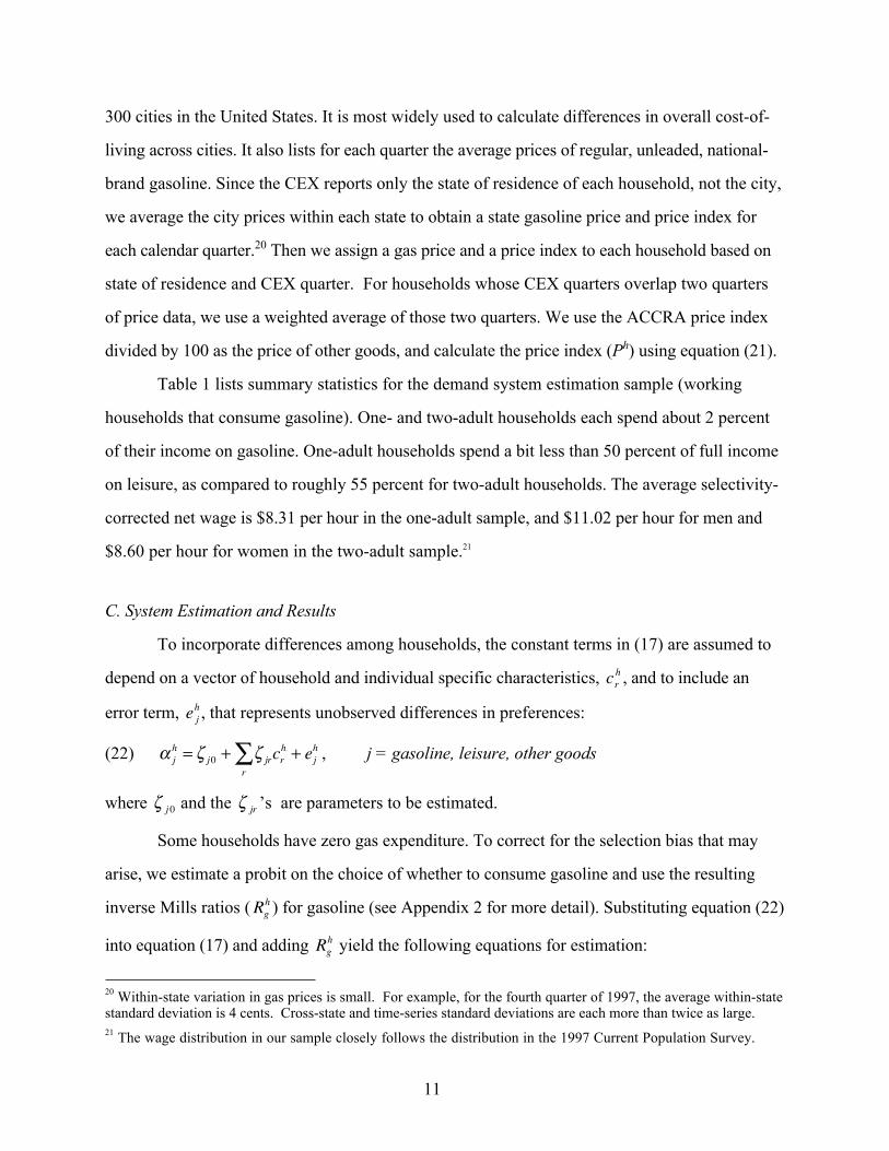
300 cities in the United States. It is most widely used to calculate differences in overall cost-of-
living across cities. It also lists for each quarter the average prices of regular, unleaded, national-
brand gasoline. Since the CEX reports only the state of residence of each household, not the city,
we average the city prices within each state to obtain a state gasoline price and price index for
each calendar quarter.20 Then we assign a gas price and a price index to each household based on
state of residence and CEX quarter. For households whose CEX quarters overlap two quarters
of price data, we use a weighted average of those two quarters. We use the ACCRA price index
divided by 100 as the price of other goods, and calculate the price index (Ph) using equation (21).
Table 1 lists summary statistics for the demand system estimation sample (working
households that consume gasoline). One- and two-adult households each spend about 2 percent
of their income on gasoline. One-adult households spend a bit less than 50 percent of full income
on leisure, as compared to roughly 55 percent for two-adult households. The average selectivity-
corrected net wage is $8.31 per hour in the one-adult sample, and $11.02 per hour for men and
$8.60 per hour for women in the two-adult sample.21
C. System Estimation and Results
To incorporate differences among households, the constant terms in (17) are assumed to
depend on a vector of household and individual specific characteristics,
�
crh , and to include an
error term,
�
e jh , that represents unobserved differences in preferences:
(22) α jh = ζ j0 + ζ jrcr
h
r∑ + ej
h , j = gasoline, leisure, other goods
where
�
ζ j 0 and the
�
ζ jr ’s are parameters to be estimated.
Some households have zero gas expenditure. To correct for the selection bias that may
arise, we estimate a probit on the choice of whether to consume gasoline and use the resulting
inverse Mills ratios (
�
Rgh ) for gasoline (see Appendix 2 for more detail). Substituting equation (22)
into equation (17) and adding
�
Rgh yield the following equations for estimation:
20 Within-state variation in gas prices is small. For example, for the fourth quarter of 1997, the average within-statestandard deviation is 4 cents. Cross-state and time-series standard deviations are each more than twice as large.21 The wage distribution in our sample closely follows the distribution in the 1997 Current Population Survey.

12
(23)
�
s jh = ζ j 0 + ζ jrcr
h
r∑ + γ jk log pk
h + β j log yh Ph( )
k∑ + θ jRg
h + e jh .
We estimate the demand system defined by (23) using working households that consume
gasoline, separately for one-adult and two-adult households. We impose the restrictions in (19a-
d) and drop the equation for other goods. The vector
�
crh includes member and household
characteristics that may affect gasoline or leisure shares: the members’ age, age squared, race, sex
(in one-adult estimation only), education, and number of children.22 In addition, a wide range of
local factors could affect gasoline use or work behavior–everything from availability of public
transportation to local urban design to cultural differences. Because many of these factors are
unmeasurable, we include state fixed effects to account for them. Finally, to account for seasonal
variation in gas demand, we include fixed effects for the month of the CEX interview.
Under this approach, the own-price gas demand elasticity is identified based on cross-
state differences in quarter-to-quarter gas price variation, because cross-state variation is picked
up by the state fixed effects and month-to-month variation by the month fixed effects. The own-
and cross-price labor supply elasticities are identified primarily by cross-section wage variation
within each state.23 This requires the implicit assumption that unobserved household
characteristics are not correlated both with wages and with gas consumption or hours worked.
We use instrumental variables to control for potential endogeneity. The net wage may be
endogenous for two reasons. First, the gross wage is determined by dividing earnings by hours of
work, and both variables may be measured with error. Thus, hours worked and wage rates may
be correlated. Second, the marginal income tax rate depends on income. We therefore instrument
for the net wage rate with its occupation-, state-, and gender-specific mean.24
The real income term ln(yh/Ph) may also be endogenous, because it is a function of
individual-specific shares that are also dependent variables. We instrument for this term, using an
22 The probits used to correct for selectivity each include at least one variable not included in the demand system.23 It might therefore seem that we estimate long-run labor supply elasticities and short-run gas demand elasticties.But since the coefficients are jointly estimated, none of our elasticities is strictly short-run or long-run.24 Observations for workers in two occupation categories (farming, forestry, fishing, and groundskeeping is the firstand the armed forces the second) are spread very thinly across states. For workers with these occupations, weinstrument for net wage with the national mean net wages by occupation rather than the state level means.

13
alternative price index obtained by replacing the individual-specific shares in (21) with the sample
mean shares.25 Finally, gas prices may be endogenous, but we do not control for this potential
endogeneity because we lack a good instrument for state-level gas prices.26
Since the equations in (23) are functions of the same explanatory variables, error terms are
likely correlated across equations. We therefore use three-stage least squares (3SLS), which lets
us impose the cross-equation restrictions in (19a-d), control for endogeneity with instrumental
variables, and account for the error correlation structure using generalized least squares.27
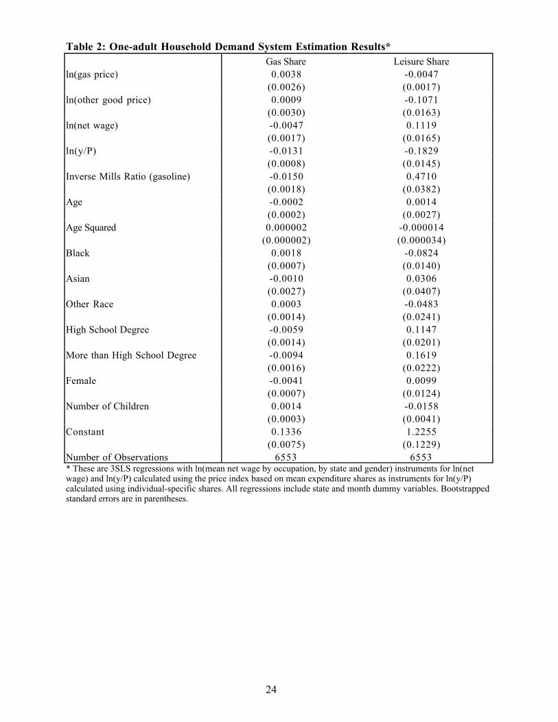
Tables 2 and 3 present the system estimation results along with standard errors based on
1500 replications of a nonparametric bootstrap. Each bootstrap replication recomputes the
Heckman-corrected wage and the inverse Mills ratios from the discrete choice of whether to
consume gasoline, as well as the regression coefficients. Thus, the standard error estimates
incorporate variation in the estimated selectivity-corrected wages and inverse Mills ratios.
Because observations for the same household for multiple quarters are not independent, we
cluster observations by household in generating each bootstrap sample.
Among one-adult households, gas share is higher for blacks, males, and those with less
education, more children, or higher wages. Leisure share is lower for blacks and those with less
education or more children. Higher wages or higher prices for other goods reduce leisure share,
while higher gas prices increase it. The two-adult estimates generally mirror the one-adult
estimates, though the magnitudes differ. The share of leisure (for either adult) increases as his or
her wage increases and decreases as the wage of the other adult in the household increases.
Tables 4 and 5 present elasticities for the one-adult and two-adult samples, respectively,
25 We also estimate our system using this alternative index instead of the index in (21). This does not noticeablyaffect any of the results, nor does running the demand system without any instruments at all.26Because we include state fixed effects, state-level gas tax rates are poor instruments for gas prices, explaining onlyabout 1 percent of gas price variation. We also do not correct for the potential endogeneity of fuel efficiency. West(2004) uses similar data to estimate demand for miles driven and finds that accounting for this endogeneity resultsin less elastic demand. The more inelastic is gas demand, the larger will be the effect of the cross-price elasticitywith leisure on the optimal tax rate. Thus, correcting for this endogeneity would likely strengthen our findings.27 In principle, the full econometric model, including all discrete and continuous choices, might be estimated usingmaximum likelihood, but this would be difficult to implement. Since censoring occurs in both gasoline and leisuredemand, and for either or both the male and female in two-adult households, we would need to evaluate multipleintegrals in the likelihood function. Such a procedure would probably be too computationally intensive to bepractical, particularly given that we need to bootstrap standard errors for our elasticity and optimal tax estimates.

14
along with bias-corrected bootstrap confidence intervals. These elasticities are calculated
separately for each household and then aggregated, rather than being calculated for a
representative household.28 Compensated own-price gas and other-good demand elasticities are
negative, and compensated own-wage labor elasticities are positive. Gasoline own-price
elasticity estimates are roughly –0.75 for one-adult households and -0.27 for two-adult
households, which fall in the span of estimates reported in gas demand surveys.29
For one-adult households, the compensated and uncompensated labor supply elasticities
are 0.35 and 0.04, respectively. For two-adult households, compensated own-wage labor supply
elasticities are 0.19 for men and 0.34 for women, while uncompensated elasticities are 0.06 and
0.24. These fall into the range reported in the survey by Fuchs et al. (1998).
The other important elasticity in equation (15) is the uncompensated cross-price
elasticity of labor with respect to the price of gasoline. A positive value for this elasticity raises
the optimal gas tax, because in this case an increase in the price of gasoline discourages leisure –
which is overconsumed because it is untaxed – thus yielding a welfare gain. A negative value
reverses this effect, lowering the optimal tax. The prior literature on optimal environmental taxes
has implicitly assumed that this elasticity is slightly negative, as a result of assuming separability
and homogeneity. In contrast, we find a positive elasticity for one-adult households and for both
genders in two-adult households, which implies a higher optimal gas tax rate than that suggested
by prior work – though the elasticity is significant only for men in two-adult households.30
One possible explanation for this result is that a higher gas price leads to a reduction in
leisure driving that is substantially greater than the reduction in work-related driving (primarily
28 In most cases, aggregate demand elasticities under the AIDS are equal to the elasticity for a representativehousehold, but that property does not hold when some households are at a corner solution, as is the case here.Thus, it is necessary to aggregate individual household elasticities. Appendix 1 provides equations for thehousehold demand elasticities in terms of the estimated parameters and for elasticity aggregation.29 See Dahl and Sterner (1991) or Espey (1996).30 This result is sensitive to the inclusion of state fixed effects: dropping the state fixed effects switches the sign onthe elasticity of labor supply with respect to the gas price from positive (meaning gas and leisure are complements)to negative (gas and leisure are substitutes). But this sensitivity is hardly surprising, given the importance ofunobserved state-level variables; joint significance tests overwhelmingly reject dropping state fixed effects. Incontrast, dropping month fixed effects has little effect on the results. Because estimates from 3SLS estimation areoften very sensitive to specification error, we also estimated the system using two-stage least squares (2SLS).Estimates using 2SLS with and without fixed effects closely follow those from the same specifications using 3SLS.

15
commuting). Parry and Small (2005) note that commuting makes up less than half of all vehicle
miles traveled in the US, and it is reasonable to think that the demand for leisure driving would be
more elastic than the demand for work-related driving.31 A more sophisticated argument is that
driving is a relatively time-intensive activity (at the margin, once households have incurred the
fixed cost of buying a car). Becker’s (1965) model of time use suggests that time-intensive goods
are complements to leisure (or, more precisely, to non-market time).
III. Optimal Tax Calculations
This section calculates the optimal gasoline tax rate and compares it to the optimal rates
that would be implied by each of the sets of assumptions used in prior work: fixed labor supply,
homotheticity and separability of leisure, or just separability.
Our data set provides values for most of the variables in the formulas for the optimal tax
rate (15) and the marginal cost of public funds (14), while the estimates from the previous section
allow us to calculate the necessary derivatives of demand.32 The only additional parameter value
needed is for marginal external damage. We take this value from Parry and Small (2005), who
estimate marginal damages at 83 cents per gallon in year 2000 dollars, a figure that incorporates
pollution, congestion and accident externalities. To make this number consistent with the rest of
our data, we use the CPI to deflate it, yielding an estimate of 77 cents in 1997 dollars.33
If labor supply were fixed, then the optimal tax would simply equal marginal damage.
But allowing labor supply to vary leads to efficiency effects in the labor market, as well as in the
31 We cannot test this hypothesis because our data do not distinguish gas used for leisure driving from that used forwork-related driving. We assume that the government also cannot distinguish these two, and thus cannot tax themdifferently. If it could, then differences in cross-price effects on labor supply would suggest that gas used for work-related driving should be taxed at a lower rate than gas used for leisure driving. But differences in marginal damageact in the opposite direction, since the congestion externality is larger for work-related driving (because it is morelikely to occur during peak travel times). Thus, it is unclear which type of driving should face the higher tax rate.32 We assume that the derivatives of demand at the optimum are the same as those in the status quo. In addition,equation (15) depends on the total derivative of gas demand, which includes the effects of both gas tax and incometax changes. But this derivative is very close to the compensated derivative, and thus we use that value. Finally,for consistency with Section I, where the externality came from consumption of a final good, we assume that the taxis imposed only on consumer use of gasoline, not on gas used as an intermediate good. This seems reasonable,since Parry and Small (2005) note that intermediate use of gasoline is only a very small share of the total.33 We assume that marginal damage remains constant as the gas tax rate changes. It seems clear how certainelements of marginal damage would change (e.g., a higher gas tax will discourage driving, and thus will reduce themarginal external congestion cost). But whether marginal damage would rise or fall overall is far less clear.
16
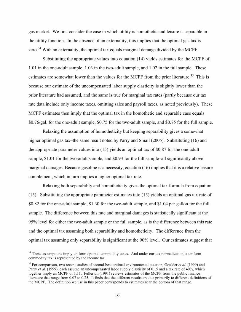
gas market. We first consider the case in which utility is homothetic and leisure is separable in
the utility function. In the absence of an externality, this implies that the optimal gas tax is
zero.34 With an externality, the optimal tax equals marginal damage divided by the MCPF.
Substituting the appropriate values into equation (14) yields estimates for the MCPF of
1.01 in the one-adult sample, 1.03 in the two-adult sample, and 1.02 in the full sample. These
estimates are somewhat lower than the values for the MCPF from the prior literature.35 This is
because our estimate of the uncompensated labor supply elasticity is slightly lower than the
prior literature had assumed, and the same is true for marginal tax rates (partly because our tax
rate data include only income taxes, omitting sales and payroll taxes, as noted previously). These
MCPF estimates then imply that the optimal tax in the homothetic and separable case equals
$0.76/gal. for the one-adult sample, $0.75 for the two-adult sample, and $0.75 for the full sample.
Relaxing the assumption of homotheticity but keeping separability gives a somewhat
higher optimal gas tax–the same result noted by Parry and Small (2005). Substituting (16) and
the appropriate parameter values into (15) yields an optimal tax of $0.87 for the one-adult
sample, $1.01 for the two-adult sample, and $0.93 for the full sample–all significantly above
marginal damages. Because gasoline is a necessity, equation (16) implies that it is a relative leisure
complement, which in turn implies a higher optimal tax rate.
Relaxing both separability and homotheticity gives the optimal tax formula from equation
(15). Substituting the appropriate parameter estimates into (15) yields an optimal gas tax rate of
$0.82 for the one-adult sample, $1.30 for the two-adult sample, and $1.04 per gallon for the full
sample. The difference between this rate and marginal damages is statistically significant at the
95% level for either the two-adult sample or the full sample, as is the difference between this rate
and the optimal tax assuming both separability and homotheticity. The difference from the
optimal tax assuming only separability is significant at the 90% level. Our estimates suggest that
34 These assumptions imply uniform optimal commodity taxes. And under our tax normalization, a uniformcommodity tax is represented by the income tax.35 For comparison, two recent studies of second-best optimal environmental taxation, Goulder et al. (1999) andParry et al. (1999), each assume an uncompensated labor supply elasticity of 0.15 and a tax rate of 40%, whichtogether imply an MCPF of 1.11. Fullerton (1991) reviews estimates of the MCPF from the public financeliterature that range from 0.07 to 0.25. It finds that the different results are due primarily to different definitions ofthe MCPF. The definition we use in this paper corresponds to estimates near the bottom of that range.

17
gasoline is not just a weaker substitute for leisure than are other goods, but that it is actually a
complement to leisure: that increasing the gasoline tax will increase labor supply (even before
considering the effects of the income tax cut financed by that gas tax increase). As a result, the
optimal tax is substantially higher than it would be if gas were an average substitute for leisure.
The difference between the optimal tax and marginal damage – 27 cents per gallon (35% of
marginal damage) for the full sample – is not enormous, but is quite important. And this
difference has the opposite sign from what the prior literature on second-best optimal
environmental taxation suggests. That literature certainly notes the theoretical possibility that
the optimal tax may exceed marginal damage, for exactly the reasons found here, but gives no clear
indication of how likely such an outcome might be or of how large the difference would be.
These results show that the separability and homotheticity assumptions (which are
common in the second-best environmental tax literature) can be very important. Relaxing these
estimates leads to a 29-cent increase (from $0.75 to $1.04) in the optimal tax. This is more than
ten times the difference between marginal damage and the optimal tax rate with separability and
homotheticity ($0.77 vs. $0.75)–which has been the major focus of this literature.
Even if there were no negative externalities associated with gasoline (i.e., if we set
marginal damage to zero), the optimal tax rate would still equal $0.28 (33% of the average pre-tax
price in our sample). This implies the existence of a “double dividend” (a welfare increase even
when externalities are ignored) from raising the gas tax above zero, but not from raising it above
the average rate in our sample ($0.34).36 However, the 95% confidence interval for the optimal
tax in this case runs from $0.11 to $0.72, so we cannot reject the hypothesis that raising the gas
tax would yield a double dividend–or, to put it differently, that the optimal gas tax would exceed
the average rate in our sample even if there were no externalities associated with gasoline use.
In this no-externality case, slightly less than half of the optimal tax ($0.11, which is 13%
of the average pre-tax price) is due to nonseparability. Thus, a study that assumes separability
(as does nearly all prior empirical work on optimal taxes) would find an “optimal” tax rate that is
36 It is well-known that a tax reform that moves one tax closer to its optimal rate does not necessarily yield awelfare gain (e.g., see Dixit, 1975). But that result doesn’t apply here: because our model includes only twoconsumption goods, such a reform will always yield a welfare gain.

18
only just over half of the correct value–a substantial underestimate.37
IV. Conclusions
This paper estimates a complete consumer demand system without imposing separability
or homotheticity, and applies those estimates together with a simple theoretical model to
calculate the optimal tax on gasoline. We find that even if there were no negative externalities
associated with gas use, the optimal gas tax would still be roughly 33% of the pre-tax price of
gasoline, almost equal to the average tax rate in our sample. This is more than one-and-a-half
times the “optimal” rate that would be implied if one were to assume that leisure is separable in
utility, as nearly all prior studies have assumed. When we include externalities, we find that the
optimal tax substantially exceeds marginal damage, contrary to results from the prior literature,
which suggest that optimal environmental taxes are typically less than marginal damage.
Thus, our results clearly illustrate the importance of explicitly estimating cross-price
elasticities with leisure rather than imposing restrictive assumptions in order to determine those
elasticities. This has important implications both for environmental regulation and for
commodity taxation.
One obvious implication is that the efficiency gain from increasing the gas tax would be
even larger than a first-best analysis would indicate. But the practical relevance of any result on
optimal gasoline taxes may be limited by political constraints; the existing tax in the U.S. is far
below what almost any economic analysis would indicate as the optimum.
Some readers may be tempted to use our results to support setting other environmental
taxes at levels above marginal damages. This conclusion does not necessarily follow, given that
other polluting goods are used for very different purposes than is gasoline. But our result does
show that the case in which tax-interaction effects cause the optimal tax to exceed marginal
damages is relevant in practice, not merely a theoretical possibility. This indicates far more
uncertainty about the influence of second-best effects on environmental policy than prior work
37 All of these optimal tax calculations ignore distributional considerations. Including such considerations wouldlower the estimated optimal tax rates, because the gas tax is regressive. But the optimal tax rate assumingseparability would fall by the same amount as the optimal tax without separability, and thus the difference betweenthe two would be unchanged.

19
has suggested, and it shows that the widely used separability and homotheticity assumptions are
not merely convenient simplifications; they can have large effects on the results. Similarly,
results from the prior literature on commodity taxation should be interpreted with caution,
because they rely on the assumption that leisure is separable in utility, which we have shown can
substantially affect estimates of optimal tax rates.
Perhaps most importantly, our results suggest that future research–either on commodity
taxation, environmental regulation, or in any of the other settings in which cross-price effects
with leisure have been shown to affect optimal policy–needs to explicitly estimate those cross-
price effects in order to yield accurate estimates of optimal policy.

20
References
Abbott, Michael and Orley Ashenfelter, 1976. “Labour Supply, Commodity Demand and theAllocation of Time.” Review of Economic Studies 43:389-411.
Ahmad, Ehtisham and Nicholas Stern, 1984. “The Theory of Reform and Indian Indirect Taxes.”Journal of Public Economics 25:259-298.
Atkinson, Anthony, and Joseph Stiglitz, 1972. “The Structure of Indirect Taxation and EconomicEfficiency.” Journal of Public Economics 1:97-119.
Ballard, Charles, John Goddeeris, and Sang-Kyum Kim, 2005. “Non-Homothetic Preferences andthe Non-Environmental Effects of Environmental Taxes.” International Tax and PublicFinance, forthcoming.
Barnett, William A., 1979. “The Joint Allocation of Leisure and Goods Expenditure.”Econometrica 47:539-563.
Becker, Gary, 1965. “A Theory of the Allocation of Time.” Economic Journal 75:493-517.
Blundell, Richard, Panos Pashardes, and Guglielmo Weber, 1993. “What Do We Learn AboutConsumer Demand Patterns from Micro Data?” American Economic Review 83:570-597.
Bovenberg, A. Lans and Ruud de Mooij, 1994. “Environmental Levies and DistortionaryTaxation.” American Economic Review 85:1085-1089.
Bovenberg, A. Lans and Lawrence Goulder, 1996. “Optimal Environmental Taxation in thePresence of Other Taxes: General Equilibrium Analyses.” American Economic Review96:985-1000.
Bovenberg, A. Lans and Frederick van der Ploeg, 1994. “Green policies and public finance in asmall open economy.” Scandinavian Journal of Economics 96:343-63.
Browning, Edgar, 1997. “A Neglected Welfare Cost of Monopoly–And Most Other ProductMarket Distortions.” Journal of Public Economics 66:127-144.
Browning, Martin and Costas Meghir, 1991. “The Effects of Male and Female Labor Supply onCommodity Demands.” Econometrica 59:925-951.
Corlett, W. J., and D. C. Hague, 1953. “Complementarity and the Excess Burden of Taxation.”Review of Economic Studies 21:21-30.
Dahl, Carol, and Thomas Sterner, 1991. “Analyzing Gasoline Demand Elasticities: A Survey.”Energy Economics 13:203-210.

21
Deaton, Angus and John Muellbauer, 1980. “An Almost Ideal Demand System.” AmericanEconomic Review 70:312-326.
Decoster, André, and Erik Schokkaert, 1990. “Tax Reform Results with Different DemandSystems.” Journal of Public Economics 41:277-296.
Diewert, W. Erwin, and Denis Lawrence, 1996. “The Deadweight Costs of Taxation in NewZealand.” Canadian Journal of Economics 29:S659-S673.
Dixit, Avinash, 1975. “Welfare Effects of Tax and Price Changes.” Journal of Public Economics4:103-123.
Espey, Molly, 1996. “Explaining the Variation in Elasticity Estimates of Gasoline Demand in theUnited States: A Meta-Analysis.” Energy Journal 17:49-60.
Feenberg, Daniel and Elisabeth Coutts, 1993. “An Introduction to the TAXSIM Model.”Journal of Policy Analysis and Management 12:189-194.
Fuchs, Victor, Alan Krueger and James Poterba, 1998. “Economists’ Views about Parameters,Values and Policies: Survey Results in Labor and Public Economics.” Journal ofEconomic Literature 36:1387-1425.
Fullerton, Don, 1991. “Reconciling Recent Estimates of the Marginal Welfare Cost of Taxation.”American Economic Review 81:302-308.
Fullerton, Don and Gilbert Metcalf, 2001. “Environmental Controls, Scarcity Rents, and Pre-Existing Distortions.” Journal of Public Economics 80:249-267.
Goulder, Lawrence, Ian Parry, Roberton Williams III, and Dallas Burtraw, 1999. “The Cost-Effectiveness of Alternative Instruments for Environmental Protection in a Second-BestSetting.” Journal of Public Economics, 72:329-360.
Goulder, Lawrence, and Roberton Williams III, 2003. “The Substantial Bias from IgnoringGeneral Equilibrium Effects in Estimating Excess Burden, and a Practical Solution.”Journal of Political Economy 111:898-927.
Heckman, James, 1979. “Sample Selection Bias as Specification Error.” Econometrica 47:153-161.
Jorgenson, Dale W. and Peter J. Wilcoxen, 1993. “Reducing U.S. Carbon Emissions: AnEconometric General Equilibrium Assessment.” Resource and Energy Economics 15:7-26.
Kim, Seung-Rae, 2002. "Optimal Environmental Regulation in the Presence of Other Taxes: TheRole of Non-separable Preferences and Technology." Contributions to Economic Analysis& Policy: Vol. 1: No. 1, Article 4.
22
Madden, David, 1995. “Labour Supply, Commodity Demand and Marginal Tax Reform.”Economic Journal 105:485-497.
Moschini, Giancarlo, 1995. “Units of Measurement and the Stone Index in Demand SystemEstimation.” American Journal of Agricultural Economics 77:63-68.
Parry, Ian, 1999. “Agricultural Policies in the Presence of Distorting Taxes.” American Journal ofAgricultural Economics 81:212-230.
Parry, Ian, and Kenneth Small, 2005. “Does Britain or the United States Have the Right GasolineTax?” American Economic Review, forthcoming.
Parry, Ian, Roberton Williams III, and Lawrence Goulder, 1999. “When Can Carbon AbatementPolicies Increase Welfare? The Fundamental Role of Distorted Factor Markets.” Journalof Environmental Economics and Management, 37:52-84.
Ray, Ranjan, 1986. “Sensitivity of ‘Optimal’ Commodity Tax Rates to Alternative DemandFunctional Forms: An Econometric Case Study of India.” Journal of Public Economics31:253-268.
Sandmo, Agnar, 1975. “Optimal Taxation in the Presence of Externalities.” Swedish Journal ofEconomics 77:86-98.
West, Sarah, 2004. “Distributional Effects of Alternative Vehicle Pollution Control Policies.”Journal of Public Economics 88:735-757.
Williams, Roberton, III, 1999. “Revisiting the Cost of Protectionism: The Role of TaxDistortions in the Labor Market.” Journal of International Economics, 47:429-447.
Williams, Roberton, III, 2002. “Environmental Tax Interactions When Pollution Affects Health orProductivity.” Journal of Environmental Economics and Management, 44:261-270.
Williams, Roberton, III, 2003. “Health Effects and Optimal Environmental Taxes.” Journal ofPublic Economics, 87:323-335.

23
Table 1: Summary Statistics for Working Households with Non-zero Gas Consumption*One-adult Households Two-adult Households
Variable MeanStandardDeviation Mean
StandardDeviation
Gasoline per Week (gallons) 13.78 10.97 24.67 16.07One-adult Hours per Week 41.25 10.92 - -Two-adult Male Hours per Week - - 44.76 10.34Two-adult Female Hours per Week - - 37.54 11.09Gasoline Share of Expenditures .02 .01 .02 .01One-adult Leisure Share of Expenditures .49 .11 - -Two-adult Male Leisure Share of Expenditures - - .29 .09Two-adult Female Leisure Share of Expenditures - - .26 .07Other Good Share of Expenditures .50 .15 .44 .12Gas Price ($) 1.19 .12 1.19 .11Other Good Price (index) 1.04 .10 1.04 .11One-adult Heckman-Corrected Net Wage ($) 8.31 2.36 - -Two-adult Male Heckman-Corrected Net Wage ($) - - 11.02 3.26Two-adult Female Heckman-Corrected Net Wage ($) - - 8.60 2.20ln(y/P) 5.72 .50 6.23 .45One-Adult Age (years) 37.2 11.4 - -Two-Adult Male Age (years) - - 38.5 10.0Two-Adult Female Age (years) - - 37.0 9.5One-Adult Education: < High School Diploma (%) 6.8 - - -One-Adult Education: High School Diploma (%) 23.3 - - -One-Adult Education: > High School Diploma (%) 69.9 - - -Two-Adult Male Education: < High School Diploma (%) - - 8.5 -Two-Adult Male Education: High School Diploma (%) - - 27.9 -Two-Adult Male Education: > High School Diploma (%) - - 63.6 -Two-Adult Female Education: < High School Diploma (%) - - 6.8Two-Adult Female Education: High School Diploma (%) - - 26.9 -Two-Adult Female Education: > High School Diploma (%) - - 66.4 -Race of Household Head
White (%) 82.6 - 87.5 -Black (%) 13.7 - 8.8 -Asian (%) .7 - .8 -Other race (%) 3.0 - 2.9 -
Number of Children .41 .87 1.16 1.18Region
Northeast (%) 13.3 - 13.3 -Midwest (%) 24.5 - 25.8 -South (%) 34.1 - 35.5 -West (%) 28.1 - 25.4 -
Observations 6553 - 7162 -* Of the one-adult households 46% are headed by males while 54% are headed by females.
24
Table 2: One-adult Household Demand System Estimation Results*Gas Share Leisure Share
ln(gas price) 0.0038 -0.0047(0.0026) (0.0017)
ln(other good price) 0.0009 -0.1071(0.0030) (0.0163)
ln(net wage) -0.0047 0.1119(0.0017) (0.0165)
ln(y/P) -0.0131 -0.1829(0.0008) (0.0145)
Inverse Mills Ratio (gasoline) -0.0150 0.4710(0.0018) (0.0382)
Age -0.0002 0.0014(0.0002) (0.0027)
Age Squared 0.000002 -0.000014(0.000002) (0.000034)
Black 0.0018 -0.0824(0.0007) (0.0140)
Asian -0.0010 0.0306(0.0027) (0.0407)
Other Race 0.0003 -0.0483(0.0014) (0.0241)
High School Degree -0.0059 0.1147(0.0014) (0.0201)
More than High School Degree -0.0094 0.1619(0.0016) (0.0222)
Female -0.0041 0.0099(0.0007) (0.0124)
Number of Children 0.0014 -0.0158(0.0003) (0.0041)
Constant 0.1336 1.2255(0.0075) (0.1229)
Number of Observations 6553 6553* These are 3SLS regressions with ln(mean net wage by occupation, by state and gender) instruments for ln(netwage) and ln(y/P) calculated using the price index based on mean expenditure shares as instruments for ln(y/P)calculated using individual-specific shares. All regressions include state and month dummy variables. Bootstrappedstandard errors are in parentheses.

25
Table 3: Two-adult Household Demand System Estimation Results*Gas Share Male Leisure Female Leisure
ln(gas price) 0.0102 -0.0061 -0.0031(0.0018) (0.0010) (0.0009)
ln(other good price) -0.0011 -0.0604 -0.0491(0.0020) (0.0094) (0.0075)
ln(male net wage) -0.0061 0.1383 -0.0717(0.0010) (0.0086) (0.0052)
ln(female net wage) -0.0031 -0.0717 0.1239(0.0009) (0.0052) (0.0069)
ln(y/P) -0.0090 -0.1687 -0.1694(0.0006) (0.0067) (0.0050)
Inverse Mills Ratio (gasoline) -0.0168 0.1820 0.1653(0.0024) (0.0269) (0.0212)
Male Age 0.0003 -0.0004 0.0006(0.0002) (0.0016) (0.0011)
Male Age Squared -0.000003 0.000007 -0.000004(0.000002) (0.000020) (0.000014)
Black Male -0.0006 -0.0119 -0.0091(0.0015) (0.0147) (0.0127)
Asian Male -0.0011 0.0189 0.0012(0.0018) (0.0149) (0.0146)
Other Race Male 0.0002 -0.0243 0.0087(0.0014) (0.0110) (0.0100)
Male High School Degree -0.0020 0.0132 0.0035(0.0010) (0.0064) (0.0048)
Male More than High School Degree -0.0022 0.0192 0.0067(0.0011) (0.0076) (0.0052)
Female Age 0.0005 0.0007 -0.0031(0.0002) (0.0012) (0.0013)
Female Age Squared -0.000005 -0.000006 0.000042(0.000002) (0.000016) (0.000016)
Black Female 0.0002 -0.0090 -0.0096(0.0016) (0.0149) (0.0132)
Asian Female 0.0016 0.0037 -0.0218(0.0021) (0.0237) (0.0110)
Other Race Female -0.0019 0.0235 -0.0124(0.0013) (0.0103) (0.0099)
Female High School Degree 0.0004 -0.0044 0.0103(0.0009) (0.0062) (0.0060)
Female more than High School Degree 0.0004 -0.0032 0.0205(0.0010) (0.0067) (0.0067)
Number of Children 0.0004 -0.0019 0.0075(0.0002) (0.0013) (0.0010)
Constant 0.0904 1.3480 1.4282(0.0054) (0.0565) (0.0444)
Observations 7162 7162 7162* 3SLS regressions use ln(mean net wage by occupation, by state and gender) instruments for ln(net wage) and ln(y/P)calculated using the price index based on mean expenditure shares as instruments for ln(y/P) calculated using individual-specific shares. All regressions include state and month dummy variables. Bootstrapped standard errors are in parentheses.

26
Table 4: One-Adult Elasticities
Compensated Price Elasticities Gas Price Wage Other Good Price Gasoline -0.750 0.180 0.586 (-1.095 -0.457) (0.006 0.355) (0.255 0.935) Labor -0.009 0.353 -0.296 (-0.017 -0.001) (0.261 0.459) (-0.384 -0.217) Other Good 0.0163 0.203 -0.209 (0.008 0.028) (0.115 0.229) (-0.242 -0.135)
Uncompensated Price Elasticities Gas Price Wage Other Good Price Gasoline -0.771 0.305 0.455 (-1.088 -0.479) (0.131 0.474) (0.084 1.094) Labor 0.003 0.040 0.024 (-0.005 0.011) (-0.066 0.168) (-0.074 0.128) Other Good -0.005 0.621 -1.009 (-0.014 0.005) (0.356 0.665) (-1.075 -0.947)Bias-corrected 95% confidence intervals are in parentheses, based on 1500 replications of anonparametric clustered bootstrap.

27
Table 5: Two-Adult Elasticities
Compensated Price Elasticities Gas Price Male Wage Female Wage Other Good Price Gasoline -0.269 -0.123 0.042 0.354 (-0.538 -0.011) (-0.269 0.003) (-0.051 0.140) (0.061 0.639) Male 0.007 0.187 0.012 -0.181Labor (0.000 0.015) (0.105 0.272) (-0.018 0.042) (-0.256 -0.096) Female -0.005 0.028 0.337 -0.321Labor (-0.016 0.005) (-0.030 0.087) (0.252 0.427) (-0.415 -0.241) Other 0.012 0.102 0.095 -0.201Good (0.002 0.021) (0.048 0.141) (0.070 0.123) (-0.255 -0.134)
Uncompensated Price Elasticities
Gas Price Male Wage Female Wage Other Good Price Gasoline -0.283 0.011 0.110 0.178 (-0.540 -0.021) (-0.133 0.134) (0.020 0.213) (-0.285 0.646) Male 0.013 0.062 -0.049 -0.045Labor (0.006 0.022) (-0.019 0.152) (-0.080 -0.019) (-0.126 0.043) Female 0.002 -0.113 0.242 -0.165Labor (-0.008 0.013) (-0.174 -0.055) (0.158 0.329) (-0.252 -0.076) Other -0.016 0.548 0.328 -1.090Good (-0.026 -0.007) (0.314 0.588) (0.295 0.362) (-1.154 -1.003)Bias-corrected 95% confidence intervals are in parentheses, based on 1500 replications of anonparametric clustered bootstrap.

28
Table 6: Estimated Optimal Tax Rates (in 1997 dollars)
(One-Adult Households Only) MED MCPF Optimal Tax Rate
Fixed labor supply $0.77 1 $0.77
Labor supply not fixed $0.77 1.01 $0.76
(utility separable & homothetic) (0.99 1.03) ($0.74 $0.78)
Labor supply not fixed (utility $0.77 1.01 $0.87separable, nonhomothetic) (0.99 1.03) ($0.83 $0.92)
Labor supply not fixed (utility $0.77 1.01 $0.82nonseparable, nonhomothetic) (0.99 1.03) ($0.73 $0.95)
(Two-Adult Households Only) MED MCPF Optimal Tax Rate
Fixed labor supply $0.77 1 $0.77
Labor supply not fixed $0.77 1.03 $0.75
(utility separable & homothetic) (1.00 1.05) ($0.73 $0.77)
Labor supply not fixed (utility $0.77 1.03 $1.01separable, nonhomothetic) (1.00 1.05) ($0.66 $3.30)
Labor supply not fixed (utility $0.77 1.03 $1.30nonseparable, nonhomothetic) (1.00 1.05) ($0.82 $5.34)
(All Households) MED MCPF Optimal Tax Rate
Fixed labor supply $0.77 1 $0.77
Labor supply not fixed $0.77 1.02 $0.75
(utility separable & homothetic) (1.00 1.04) ($0.74 $0.77)
Labor supply not fixed (utility $0.77 1.02 $0.93separable, nonhomothetic) (1.00 1.04) ($0.84 $1.18)
Labor supply not fixed (utility $0.77 1.02 $1.04nonseparable, nonhomothetic) (1.00 1.04) ($0.87 $1.48)
All monetary values are in 1997 dollars. Bias-corrected 95% confidence intervals are in parentheses,based on 1500 replications of a nonparametric clustered bootstrap. Marginal external damage (MED)includes congestion and accident damages as well as environmental damages. MED estimates aretaken from Parry and Small (2005) and deflated from 2000 to 1997 dollars.

A-1
Appendix 1: Derivations and Elasticity Formulas (Not intended for publication)
Derivation of Equation (14)
It is useful first to find expressions for how
�
τ L and T change for a change in
�
τY . Taking a
total derivative of (9) with respect to
�
τY and substituting in (5) and (6) yield
(A1)
�
dτ Lhi
dτY= whi
1− τY and
�
dΤh
dτY= Ih
1− τY.
To derive an expression for the aggregate change in utility from a change in
�
τY , take the
total derivative of utility (1) with respect to
�
τY , sum over households, substitute in the first-
order conditions (10) and a total derivative of the consumer budget constraint (3) with respect to
�
τY , and rearrange terms. Note that the definition of the MCPF in (14) includes only effects in
the labor market, so we ignore the externality term in (1). This gives
(A2)
�
1λhdUh
dτYh∑ = − dTh
dτY+ Lhi
i∑ dτ L
hi
dτY
⎡
⎣ ⎢
⎤
⎦ ⎥
h∑ .
To derive an expression for the change in government revenue from a change in
�
τY , take
the total derivative of the left-hand side of the government budget constraint (8) with respect to
�
τY and rearrange terms. Again, (14) includes only effects in the labor market, so we ignore the
revenue from the tax on the polluting good. This gives
(A3)
�
d τ LhiLhi
i∑ + Th⎡
⎣ ⎢
⎤
⎦ ⎥
h∑ dτY = dTh
dτY+ Lhi dτ L
hi
dτY+ τ L
hi ∂lhi
∂IhdTh
dτY+ τ L
hi ∂lhi
∂whjdτ L
hj
dτYj∑
⎛
⎝ ⎜ ⎜
⎞
⎠ ⎟ ⎟
i∑
⎡
⎣ ⎢ ⎢
⎤
⎦ ⎥ ⎥ h
∑ .
Dividing (A2) by (A3) and then substituting in (A1) and (3) give (14).
Rewriting Equation (12) in Terms of the MCPF
The total derivative
�
dli
dτD depends on how the income tax adjusts to hold government
revenue constant. Taking a total derivative of the government budget constraint (8), substituting
in (A1) and the equation for the MCPF (14) and rearranging yield
(A4)
�
dτYdτD
= − 1− τY( )η Dh + τDdDh
dτD− τ L
hi ∂lhi
∂pDh
i∑
⎡
⎣ ⎢
⎤
⎦ ⎥
h∑ Y h
h∑ .
A-2
Substituting together
�
dlhi
dτD= ∂lhi
∂pDh − ∂lhi
∂whidτ L
hi
dτYdτYdτD
− ∂lhi
∂IhdTh
dτYdτYdτD
, (A1) and (A4) yields
(A5) τ Lhi dlhi
dτDi∑
h∑ = − η −1( ) Dh + τD
dDh
dτD
⎛⎝⎜
⎞⎠⎟−η τ L
hi ∂lhi
∂ pDh
i∑
⎡
⎣⎢
⎤
⎦⎥
h∑ .
Substituting this equation into (12) and canceling terms give
(A6)1λh
dUh
dτDh∑ = ητD −θ( ) dD
h
dτD+ η −1( )Dh −η τ L
hi ∂lhi
∂ pDh
i∑⎡
⎣⎢
⎤
⎦⎥
h∑ .
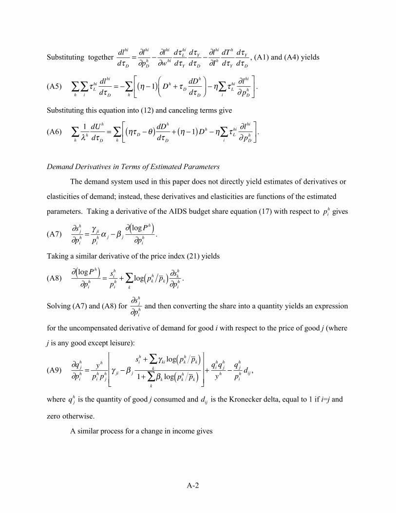
Demand Derivatives in Terms of Estimated Parameters
The demand system used in this paper does not directly yield estimates of derivatives or
elasticities of demand; instead, these derivatives and elasticities are functions of the estimated
parameters. Taking a derivative of the AIDS budget share equation (17) with respect to
�
pih gives
(A7)
�
∂s jh
∂pih =
γ ji
pih α j −β j
∂ logPh( )∂pi
h .
Taking a similar derivative of the price index (21) yields
(A8)
�
∂ logPh( )∂pi
h = sih
pih + log pk
h p k( )k∑ ∂sk
h
∂pih .
Solving (A7) and (A8) for
�
∂s jh
∂pih and then converting the share into a quantity yields an expression
for the uncompensated derivative of demand for good i with respect to the price of good j (where
j is any good except leisure):
(A9)
�
∂q jh
∂pih = yh
pih p j
h γ ji −β j
sih + γ ki log
k∑ pk
h p k( )1+ βk log
k∑ pk
h p k( )
⎡
⎣
⎢ ⎢ ⎢
⎤
⎦
⎥ ⎥ ⎥
+qi
hq jh
yh −q j
h
pih dij ,
where
�
q jh is the quantity of good j consumed and dij is the Kronecker delta, equal to 1 if i=j and
zero otherwise.
A similar process for a change in income gives

A-3
(A10)
�
∂q jh
∂yh = 1p j
h
β j
1+ βk logk∑ pk
h p k( )
⎡
⎣
⎢ ⎢ ⎢
⎤
⎦
⎥ ⎥ ⎥
+q j
h
yh .
It is then straightforward to use the Slutsky equation to obtain the compensated
derivative of demand for good i with respect to the price of good j, which is given by
(A11)
�
∂q jCh
∂pih = yh
pih p j
h γ ji + β j
γ ki logk∑ pk
h p k( )1+ βk log
k∑ pk
h p k( )
⎡
⎣
⎢ ⎢ ⎢
⎤
⎦
⎥ ⎥ ⎥
+qi
hq jh
yh −q j
h
pih dij ,
where the subscript C denotes a compensated derivative.
Correcting Derivatives for Corner Solutions
The expressions in (A9-A11) are valid for a household that is at an interior solution, but
not for those at corner solutions (i.e., those households who don’t consume gasoline, or where
one or both adults do not work). The parameter estimates should still be valid for these
households (because of the corrections for selectivity described in Appendix 2), but the
expressions for derivatives in terms of the estimated parameters will differ. We follow the
standard “virtual price” approach, recognizing that a household at a corner will have a shadow
price for the good that it is not consuming (or, in the case of leisure, that it is consuming its entire
endowment of) that differs from the true price, as a result of the constraint imposed by the
corner. This implies that if a household is constrained in its consumption of good k then
(A12)
�
∂ ˆ q jCh
∂pih =
∂q jCh
∂pih −
∂q jCh
∂pkh
∂qkCh
∂pih
∂qkCh
∂pkh
⎛
⎝ ⎜
⎞
⎠ ⎟ ,
where the “hat” denotes the derivative after correcting for the corner solution. Similarly,
(A13)
�
∂ ˆ q jCh
∂yh =∂q jC
h
∂yh −∂q jC
h
∂pkh
∂qkCh
∂yh∂qkC
h
∂pkh
⎛
⎝ ⎜
⎞
⎠ ⎟ .
Because consumption of good k is constrained, derivatives of demand for good k, or with respect
to the price of good k will equal zero.38 It is then straightforward to apply the Slutsky equation
38 If a household is at a corner solution for two goods, then this approach can be applied sequentially for the twogoods.

A-4
to obtain uncompensated derivatives (recognizing that the income effect for leisure will differ,
because the household starts with an endowment of leisure).
Aggregating Elasticities
We report aggregate elasticities in Tables 4 and 5 to clarify what is driving the optimal tax
results. Thus, it is necessary to aggregate individual household demand derivatives to obtain
aggregate elasticities. In doing this, we calculate the elasticity for a case in which each household
faces the same absolute change in price.39 This implies that the aggregate demand elasticity is
given by
(A14)
�
ε ji = p i∂q j
h
∂pih
h∑ q j
h
h∑ ,
where
(A15)
�
p i = pihqi
h
h∑ qi
h
h∑
(note that this is the same average price that is used in computing the price index in (21). The
equations for aggregate labor supply elasticities differ slightly, in that the quantities in (A14) and
(A15) are replaced with the amount of labor supplied.
39 The reported elasticities are obviously somewhat sensitive to this assumption–because households initially facedifferent prices, an equal-percentage change in price would give a slightly different result–and it is not entirely clearwhich assumption would be more appropriate. Fortunately, this has no effect on the optimal tax results, becausethe optimal tax formula in (15) is calculated using individual household demand derivatives, not aggregates.

A-5
Appendix 2: Correcting for Selectivity Bias (Not intended for publication)
This section explains corrections made for potential selection into work and into gasoline
consumption. Results for the estimation discussed here are available from the authors by request.
The Work Decision
Since we do not observe wages for non-workers, we follow Heckman (1979) to correct for
the associated selectivity bias. To do this, we estimate an equation for the choice of whether or
not to work jointly with an equation for the net wage, using full-information maximum likelihood.
We then use the results of this estimation to obtain estimated selectivity-corrected net wages.
We estimate selection models separately for the one-adult and two-adult sample, and
separately for men and for women within each sample. The one-adult selection equation includes
age, age squared, education, race, marital status, number of children, region, log of gas price, log of
other good price, and state-specific quarterly unemployment rates.40 The two-adult selection
equation includes those variables plus partner’s earnings and partner’s demographic information.
Because of the linear approximation to the price index (21), wages affect the price
derivatives of demand even for non-workers (though this effect is minimal), and thus we need
predicted wages for non-workers. Because occupation is an important determinant of net wage
but is observed only for workers, we run two selection models for each subsample, one to
estimate workers’ net wages and the other to estimate nonworkers’ net wages. Within each
subsample (where one such subsample, for example, is composed of women from one-adult
households) both the selection models use the same set of observations of workers and
nonworkers and identical selection equations. But the wage equations differ. To estimate net
wages for nonworkers we specify a wage equation that includes education, age, age squared, race,
marital status, region, and the inverse Mills ratio from the probits. To estimate net wages for
workers, we include those same variables plus occupation indicators. Since the wage distribution
is approximately log-normal, we define the dependent variable as the log of net wage.
These equations would be identified even if the variables in the selection equation were
40 Unemployment rates are gathered from the Bureau of Labor Statistics at www.bls.gov.

A-6
the same as those in the wage equation, but in that case, the identification would depend on the
normality assumption. Note, however, that in our specification, the selection equations include
number of children, the log of gas price, the log of the other good price, state-specific quarterly
unemployment rates, and, in the case of two-adult households, partner’s earnings; the wage
equations do not. Number of children affects the fixed cost of working and thus the participation
decision, but should not directly affect the wage; this is a standard exclusion restriction in the
labor supply literature. Our demand system allows gas and other good prices to affect the
continuous demand for leisure and thus it is reasonable to assume that they also affect the
discrete work choice. While high price regions may also be high wage regions, there is no reason
to postulate that an individual facing a high gas price or other good price will have a higher wage,
since we control for region in our wage equation. Unemployment rates proxy for job availability
in a state and thus affect the likelihood of working, but it is not clear why they would affect
wages. Partner's earnings proxy for an individual's non-wage income, but should not directly
affect an individual's wage; this is another standard exclusion restriction.
The Gasoline Decision
Another selection bias may arise because we exclude households that do not consume
gasoline from the system estimation. To correct for this potential bias, we follow an approach
analogous to the two-step version of the Heckman correction: we run probits on the dichotomous
choice to consume or not consume gasoline, calculate the inverse Mills ratio for each household,
and include that Mills ratio in each of the equations in the demand system estimation. We run
separate probits for one-adult and two-adult households. Each probit includes the log of total
goods expenditures, age, age squared, race, marital status, the number of children, region, an
indicator for whether the household owns its house, and the logs of gas price and other good
price. Demographic variables for both adults are included in the two-adult probit. Home
ownership acts as a proxy for access to credit and thus increases the likelihood of owning an
automobile and the likelihood of consuming gasoline (see West, 2004). We do not expect it to
affect the continuous choice of gasoline and therefore we use this as an exclusion restriction.