Optimal Subsampling Algorithms for Big DataRegressions

Mingyao Ai1, Jun Yu1,2, Huiming Zhang1, HaiYing Wang3

LMAM, School of Mathematical Sciences and Centerfor Statistical Science, Peking University 1

School of Mathematics and Statistics, Beijing Institute of Technology 2

Department of Statistics University of Connecticut 3

haiying.wang@uconn.edu

Abstract

To fast approximate maximum likelihood estimators with massive data, this paperstudies the optimal subsampling method under the A-optimality criterion (OSMAC)for generalized linear models. The consistency and asymptotic normality of the esti-mator from a general subsampling algorithm are established, and optimal subsamplingprobabilities under the A- and L-optimality criteria are derived. Furthermore, usingFrobenius norm matrix concentration inequalities, finite sample properties of the sub-sample estimator based on optimal subsampling probabilities are also derived. Sincethe optimal subsampling probabilities depend on the full data estimate, an adaptivetwo-step algorithm is developed. Asymptotic normality and optimality of the estimatorfrom this adaptive algorithm are established. The proposed methods are illustratedand evaluated through numerical experiments on simulated and real datasets.

Key words: generalized linear models; massive data; matrix concentration inequality.

1. Introduction

Nowadays, massive data sets are ubiquitous in many scientific fields and practices such asin astronomy, economics, and industrial problems. Extracting useful information from theselarge data sets is a core challenge for different communities including computer science,machine learning, and statistics. Over last decades, progresses have been made throughvarious investigations to meet this challenge. However, computational limitations still existdue to the faster growing pace of data volumes. For this, subsampling is a popular techniqueto extract useful information from massive data. This paper focuses on this technique andwill develop optimal subsampling strategies for generalized linear models (GLMs). Typically

1

arX

iv:1

806.

0676

1v2

[st

at.M

E]

26

Jun

2019

the maximum likelihood estimators (MLE) are found numerically by using the Newton-Raphson method. However, fitting a GLM on massive data is not an easy task throughthe iterative Newton-Raphson method, and it requires O(p2n) time in each iteration of theoptimization procedure.

An efficient way to solve this problem is the subsampling method (see Drineas et al.,2006b, as an example) as this method essentially downsizes the data volume. Drineas et al.(2011) proposed to make a randomized Hadamard transform on data and then use uniformsubsampling to take random subsamples to approximate ordinary least square estimatorsin linear regression models. Ma et al. (2015), Ma and Sun (2015) developed an effectivesubsampling method for linear regression models, which uses normalized statistical leveragescores of the covariate matrix as non-uniform subsampling probabilities. Jia et al. (2014)studied leverage sampling for GLMs based on generalized statistical leverage scores. Wanget al. (2018b) and Yao and Wang (2019) developed an optimal subsampling procedure tominimize the asymptotic mean squared error (MSE) of the resultant subsample-estimatorgiven the full data which is based on A- or L-optimality criterion in the language of optimaldesign. Wang et al. (2018a) proposed a new algorithm called information-based optimalsubdata selection method for linear regressions on big data. The basic idea is to select themost informative data points deterministically based on D-optimality without relaying onrandom subsampling. A divide-and-conquer version of the algorithm was developed in Wang(2019). Recent developments of big data subsampling method can be found in Wang et al.(2016).

Methodological investigations on subsampling methods with statistical guarantees formassive data regression are still limited when models are complex. To the best of ourknowledge, most of the existing results concern linear regression models such as in Ma et al.(2015) and Wang et al. (2018a). The optimal subsampling method in Wang et al. (2018b)and Yao and Wang (2019) is designed specifically for logistic and multinomial regressionmodels, respectively. However, only linear and logistic regressions are not enough to meetpractical needs (Czado and Munk, 2000). For example, we may need Poisson or negativebinomial distribution for count data and need Gamma or inverse Gaussian distribution fordata with non-negative responses. In addition, the aforementioned investigations did notconsider finite sample properties of subsampled estimators. In this paper, we fill these gapsby deriving optimal subsampling probabilities for GLMs, including these with non-canonicallink functions which allow for a wide range of statistical models for regression analysis.Furthermore, we will derive finite-sample upper bounds for approximation errors that canbe practically used to make the balance between the subsample size and prediction accuracy.Due to the non-natural link, our investigation is substantially distinct from the that in Wanget al. (2018b). For example, the Hessian matrix in the models considered in this paper maybe dependent on responses.

The rest of this paper is organized as follows. Section 2 introduces the model setupand derives asymptotic properties for the general subsampling estimator. Section 3 derivesoptimal subsampling strategies based on A- and L-optimality criteria for GLMs. Finite-sample error bounds are also derived in this section. Section 4 designs a two-step algorithmto approximate the optimal subsampling procedure and obtains asymptotic properties of theresultant estimator. Section 5 illustrates our methodology through numerical simulationsand a real data applications.

2

2. Preliminaries

2.1 Models and Assumptions

Recall the definition of one parameter exponential family of distributions f(y|θ) = h(y) exp(θy−ψ(θ)), θ ∈ Θ as in (5.50) of Efron and Hastie (2016), where θ is called the canonical pa-rameter and Θ is called the natural parameter space. Here f(·|θ) is a probability densityfunction for the continuous case or a probability mass function for the discrete case; h(·)is a specific function that does not depend on θ; and the parameter space Θ is defined asΘ := {θ ∈ R :

∫h(x) exp(θx)µ(dx) < ∞} with µ being the dominating measure. The ex-

ponential family includes most of the commonly used distributions such as normal, gamma,Poisson, and binomial distributions (see Efron and Hastie, 2016; Mccullagh and Nelder,1989).

A key tactic for a generalized linear regression model is to express θ in form of a linearfunction of regression coefficients. Let (x, y) be a pair of random variables where y ∈ R andx ∈ Rp. The generalized linear regression model assumes that the conditional distributionof yi given xi is determined by θi = u(βTxi). Specifically for exponential family, it assumesthat the distribution of y|x is

f(y|β,x) = h(y) exp(yu(βTxi)− ψ(u(βTxi))), with βTx ∈ Θ. (1)

The problem of interest is to estimate the unknown β from observed data. As specialcase when u(t) = t, the corresponding models are the so-called GLMs with canonical linkfunctions. Some typical examples of this type GLMs are logistic regression for binary dataand Poisson regression for count data. A commonly used GLM with non-canonical linkfunction is negative binomial regression (NBR), which is often used as an alternative toPoisson regression when data exhibit overdispersion. For this model, u(t) = t − log(ν + et)and ψ(u(t)) = ν log(ν + et) for some size parameter ν.

2.2 General Subsampling Algorithm and its Asymptotic Proper-ties

In this subsection, we study a general subsampling algorithm for GLMs and obtain someasymptotic results.

To facilitate the presentation, denote the full data matrix by Fn = (X,y), where X =(x1, . . . ,xn)T is the covariate matrix and y = (y1, . . . , yn)T is the response vector. In thispaper, we assume that (xi, yi)’s are independently generated from a GLM. Let S be a setof subsample with r data points, and define the sampling distribution πi for all data pointsi = 1, 2, ...n as π. A general subsampling algorithm follows the steps below.

1. Assign a sampling distribution π such that in each draw, the i-th element in the fulldataset Fn has the inclusion probability πi.

2. Sample with replacement r times to form the subsample set S := {(y∗i ,x∗i , π∗i ), i =1, . . . , r}, where x∗i , y

∗i , and π∗i stand for covariates, responses, and subsampling prob-

abilities in the subsample, respectively.

3

3. Based on the subsample set S, calculate the weighted log-likelihood estimator by max-imizing the following function

L∗(β) =1

r

r∑t=1

1

π∗i[y∗i u(βTx∗i )− ψ(u(βTx∗i ))]. (2)

An important feature of the above algorithm is that subsample estimator is essentially aweighted MLE and the corresponding weights are inverses of subsampling probabilities. Thisis analogous to the Hansen-Hurwitz estimator (Hansen and Hurwitz, 1943) in classic samplingtechniques. For an overview see Sarndal et al. (1992). Although Ma et al. (2015) showedthat the unweighted subsample estimator is asymptotically unbiased for β in leveragingsampling, an unweighted subsample estimator is in general biased if the sampling distributionπ depends on the responses. The inverse-probability weighting scheme is to remove bias,and we restrict our analysis on the weighted estimator here.

Let ψ(t) and ψ(t) be the first and the second derivatives of ψ(t), respectively. To charac-terize asymptotic properties of subsampled estimators, we require some regularity assump-tions listed below.

(H.1): Assume that βTx lies in the interior of a compact set K ∈ Θ almost surely.

(H.2): The regression coefficient β is a inner point of the compact domain ΛB ={β ∈ Rp : ‖β‖ ≤ B} for some constant B.

(H.3): Central moments condition: n−1∑n

i=1 |yi − ψ(u(βTxi))|4 = OP (1) for all β ∈ΛB.

(H.4): As n→∞, the observed information matrix

JX := 1n

n∑i=1

{u(βTMLExi)xixTi [ψ(u(βTMLExi))− yi]

+ψ(u(βTMLExi))u2(βTMLExi)xix

Ti ]}

goes to a positive-definite matrix in probability.

(H.5): Require that the full sample covariates have finite 6th-order moments, i.e.,E‖x1‖6≤∞.

(H.6): Assume n−2∑n

i=1 ‖xi‖k/πi = OP (1) for k = 2, 4.

(H.7): For γ = 0 and some γ > 0, assume

1

n2+γ

n∑i=1

|yi − ψi(u(βTMLExi))|2+γ‖u(βTMLExi)xi‖2+γ

π1+γi

= OP (1).

Here, assumptions (H.1) and (H.2) are the set of assumptions used in Clemencon et al.(2014). The set in (H.2) is also called admissible set which premises for consistency estima-tion for GLMs with full data (see Fahrmeir and Kaufmann, 1985). These two assumptions

4

ensure that E(yi|xi) <∞ for all i. Assumption (H.4) imposes a condition on the covariatesto make sure that the MLE based on the full dataset is consistent. To obtain the Bahadurrepresentation of the subsampled estimator, (H.3) and (H.5) are needed. Assumptions(H.6) and (H.7) are moment conditions on covariates and sub-sampling probabilities. As-sumption (H.7) is required by the Lindeberg-Feller central limit theorem. Specifically forthe uniform subsampling with πi = n−1 or more generally when maxi=1,...,n(nπi)

−1 = OP (1),

(H.7) is implied by that n−1∑n

i=1 |yi − ψi(u(βTMLExi))|2+γ‖u(βTMLExi)xi‖2+γ = OP (1), whichis guaranteed by the conditions that E|y|4+2γ = O(1) under (H.1) and (H.5).

The theorem below presents the consistency of the estimator from the subsampling algo-rithm to the full data MLE.

Theorem 1. If Assumptions (H.1)–(H.6) hold, then as n→∞ and r →∞, β is consistentto βMLE in conditional probability given Fn. Moreover, the rate of convergence is r−1/2. Thatis, with probability approaching one, for any ε > 0, there exist finite ∆ε and rε such that

P (‖β − βMLE‖ ≥ r−1/2∆ε|Fn) < ε (3)

for all r > rε.

Besides consistency, we derive the asymptotic distribution of the approximation error,and prove that the approximation error, β − βMLE, is asymptotically normal in conditionaldistribution.

Theorem 2. If Assumptions (H.1)–(H.7) hold, then as n→∞ and r →∞, conditional onFn in probability,

V −1/2(β − βMLE) −→ N(0, I) (4)

in distribution, where V = J −1X VcJ −1

X = Op(r−1) and

Vc =1

rn2

n∑i=1

{yi − ψ(u(βTMLExi))}2u2(βTMLExi)xixTi

πi. (5)

3. Optimal Subsampling Strategies

In this section, we will consider how to specify subsampling distribution π = {πi}ni=1 withtheoretical backup.

3.1 Optimal Subsampling Strategies Based on Optimal DesignCriteria

Based on A-optimality criterion in the theory of design of experiments (see Pukelsheim,2006), optimal subsampling is to choose subsampling probabilities such that the asymptoticMSE of β is minimized. This idea was proposed in Wang et al. (2018b) and we call theresulting subsampling strategy mV-optimal.

5

Theorem 3. The subsampling strategy is mV-optimal if the subsampling probability is chosensuch that

πmVi =

|yi − ψ(u(βTMLExi))|‖J −1X u(βTMLExi)xi‖∑n

j=1 |yj − ψ(u(βTMLExi))|‖J−1X u(βTMLExj)xj‖

, i = 1, 2, ..., n. (6)

The optimal subsampling probability πmV has a meaningful interpretation from the view-point of optimal design of experiments (Pukelsheim, 2006).

Note that under mild condition the “empirical information matrix” J eX = 1

n

∑ni=1[yi −

ψ(u(βTMLExi))]2u2(βTMLExi)xix

Ti and JX converge to the same limit, the Fisher information

matrix of model (1). This means that J eX − JX = oP (1). Thus, JX can be replaced by

J eX in πmV, because Theorem 2 still holds if JX is replaced by J e

X in (5). Let ηxi = [yi −ψ(u(βTMLExi))]

2u2(βTMLExi)xixTi , the contribution of the i-th observation to the empirical

information matrix, and J eXxiα

= (1−α)J eX +αηxi , which can be interpreted as a movement

of the information matrix in a direction determined by the i-th observation. The directionalderivative of tr(J e

X−1) through the direction determined by the ith observation is Fi =

limα→0+ α−1{tr(J e

X−1) − tr(J e

Xxiα−1)}. This directional derivative is used to measure the

relative gain in estimation efficiency under the A-optimality by adding the i-th observationsinto the sample. Thus, the optimal subsampling strategy prefers to select the data pointswith large values of directional derivatives, i.e., data points that will result in a larger gainunder the A-optimality.

The optimal subsampling strategy derived from mV -optimal critria requires the calcu-lation of ‖J −1

X u(βTMLExi)xi‖ for i = 1, 2, ..., n, which takes O(np2) time. To reduce thecalculating time, Wang et al. (2018b) proposed a modified optimality criterion to minimizetr(Vc). This criterion essentially is the L-optimality criterion in optimal experimental design(see Pukelsheim, 2006), which is to improve the quality of JXβ. It is easy to see that onlyO(np) time is needed to calculate the optimal sampling probabilities. We call the resultingsubsampling strategy mVc-optimal.

Theorem 4. The subsampling strategy is mVc-optimal if the subsampling probability is cho-sen such that

πmVci =

|yi − ψ(u(βTMLExi))|‖u(βTMLExi)xi‖∑nj=1 |yj − ψ(u(βTMLExj))|‖u(βTMLExj)xj‖

, i = 1, 2, ..., n. (7)

Note that in order to calculate ‖J −1X u(βTMLExi)xi‖ for i = 1, 2, ..., n, we need O(np2)

time while only O(np) time is needed to evaluate ‖u(βTMLExi)xi‖. Note that JX and Vcare nonnegative definite, and V = J −1

X VcJ −1X . Simple matrix algebra yields that tr(V ) =

tr(VcJ −2X ) ≤ σmax(J −2

X )tr(Vc), where σmax(A) denotes the maximum singular value of matrixA. Since σmax(J −2

X ) does not depend on π, minimizing tr(Vc) minimizes an upper bound oftr(V ). In fact, for two given subsampling strategies π(1) and π(2), if Vc(π

(1)) ≤ Vc(π(2)) in

the sense of Loewner-ordering, then it follows that V (π(1)) ≤ V (π(2)). Thus the alternativeoptimality criterion greatly reduces the computing time without losing too much estimationaccuracy.

Due to the score function for the log-likelihood, it is interesting that πmVci ’s in Theorem 4

are proportional to ‖{yi−ψ(βTMLExi)}u(βTMLExi)xi‖, norms of gradients of the log-likelihood

6

at individual data points evaluated at the full data MLE. This is trying to find the subsamplethat best approximate the full data score function at the full data MLE.

We now illustrate Theorem 3 and Theorem 4 with some commonly used GLMs. Notethat u(·) is the identity function for GLMs with nature link functions such as logistic andPoisson regressions. For logistic regression,

πmVi =

|yi − pi|∥∥J −1

X xi∥∥∑n

j=1 |yj − pj|∥∥J −1

X xj∥∥ , πmVc

i =|yi − pi| ‖xi‖∑nj=1 |yj − pj| ‖xj‖

,

with pi = exp(βTMLExi)/{1 + exp(βTMLExi)} and JX = n−1∑n

k=1 pk(1− pk)xkxTk . These arethe same as the results in Wang et al. (2018b). For Poisson regression,

πmVi =

|yi − λi|∥∥J −1

X xi∥∥∑n

j=1 |yj − λj|∥∥J −1

X xj∥∥ , πmVc

i =|yi − λi| ‖xi‖∑nj=1 |yj − λj| ‖xj‖

,

with λi = exp(βTMLExi) and JX = n−1∑n

k=1 exp(βTMLExk)xkxTk . NBR does not have a

canonical link function, and the conditional distribution of the response is modeled by atwo-parameter distribution

f(yi|ν, µi) =Γ(ν + yi)

Γ(ν)yi!

(µi

ν + µi

)yi ( ν

ν + µi

)ν, i = 1, 2, . . . , n,

where the size parameter ν can be estimated as a nuisance parameter. The optimal subsam-pling probabilities for NBR with size parameter ν are

πmVi =

|yi−µi|∥∥∥J−1

Xνxiν+µi

∥∥∥∑nj=1 |yj−µj |

∥∥∥∥J−1X

νxjν+µj

∥∥∥∥ , πmVci =

|yi−µi|∥∥∥ νxiν+µi

∥∥∥∑nj=1 |yj−µj |

∥∥∥∥ νxiν+µj

∥∥∥∥ ,

with µi = exp(βTMLExi) and JX = n−1∑n

k=1{ν(ν + yi)µi}/(ν + µi)2xkx

Tk .

3.2 Non-asymptotic Properties

We derive some finite sample properties of the subsample estimators based on optimal sub-sampling probabilities πmV and πmVc in this section. Results are presented in forms of excessrisks for approximating the mean responses and they hold for fixed r and n without requir-ing any quantity to go to infinity. These results show factors that affect the approximationaccuracy.

Since ψ(u(xTi β)) is the conditional expectation of the response yi given xi, we aim tocharacterize the quantity of β in prediction by examining ‖ψ(u(XT

d βMLE))− ψ(u(XTd β))‖.

This quantity is the distance between the estimated conditional mean responses based onthe full data and that based on the subsamples. Intuitively, it measures the goodness of fit inusing subsample estimator to predict the mean responses. Note that we can always improvethe accuracy of the estimator by increasing the subsample size r. Here we want to have acloser look at the effects of different quantities such as covariate matrix and data dimensionand the effect of subsample size r on approximation accuracy.

7

Let σmax(A) and σmin(A) be the maximum and minimum non-zero singular values ofmatrix A, respectively, κ(A) := σmax(A)/σmin(A). Denote ψ(u(XTβ)), the vector whosethe i-th element is ψ(u(xTi β)) and define u(XTβ) := diag{u(xT1 β), · · · , u(xTnβ)}. For theestimator β obtained from the algorithm in Section 2 based on the subsampling probabilities,πmV and πmVc, the following theorem holds.

Theorem 5. Let X denotes the design matrix consisting of subsample covariates with eachsampled element rescaled by 1/

√rπ∗i . Assume that σ2

min(u(XT β)X) ≥ 0.5σ2min(u(XT β)X),

and both σmax(u(XT β)X)/√n and σmin(u(XT β)X)/

√n are bounded. For any given ε ∈

(0, 1/3), with probability at least 1− ε, we have

‖ψ(u(XT βMLE))− ψ(u(XT β))‖

≤ 2Cu[1 +4α√

log(1/ε)√r

]√pκ2(u(XT β)X)‖[y − ψ(u(XT βMLE))]‖. (8)

where α = κ(J −1X ) for πmV and α = 1 for πmVc and Cu = sup

r∈K⊂Θ|u(r)|.

Theorem 5 not only indicates that the accuracy increases with subsample size r, whichagrees with the results in Theorem 1, but also enables us to have a closer look at theeffects of different quantities such as covariate matrix and data dimension and the effectof subsample size r on approximation accuracy. Heuristically, the condition number ofu(XT β)X measures the collinearity of covariates in the full data covariate matrix; p showsthe curse of dimensionality; and ‖y − ψ(u(XT βMLE))‖ measures the goodness of fit of theunderlying model on the full data.

The result in (8) also indicates that we should choose r ∝ p to control the error bound,hence it seems reasonable to choose the subsample size as r = cp. This agrees with therecommendation of choosing a sample size as large as 10 times of the number of covariatesin Chapman et al. (1994) and Loeppky et al. (2009) for designed experiments. However,for designed experiments, covariate matrices are often orthogonal or close to be orthogonal,so κ(u(XT β)X) is equal or close to 1 in these cases. For the current paper, full datamay not be obtained from well designed experiments so u(XT β)X may vary a lot. Thus,κ(u(XT β)X) should also be considered in determining required subsample size for a givenlevel of prediction accuracy.

The particular constant 0.5 in Theorem 5’s condition σ2min(u(XT β)X) ≥ 0.5σ2

min(u(XT β)X)can be replaced by any constant between 0 and 1. Here we follow the setting of Drineas et al.(2011) and choose 0.5 for convenience. This condition indicates that the rank of u(XT β)Xis the same as that of u(XT β)X. More details and interpretations about this condition canbe found in Mahoney (2012).

Using similar argument as in the proof of Theorem 5, it is proved that this conditionholds with high probability.

Theorem 6. Let u(XT β)X denote the design matrix consisting of subsamples with eachsampled element rescaled by 1/

√rπ∗i . Assume that |yi − ψ(u(βTMLExi))|‖u(βTMLExi)xi‖ ≥

γ‖xi‖ for all i and σmax(u(XT β)X)/√n, σmin(u(XTβ)X)/

√n are bounded. For any given

ε ∈ (0, 1/3), let cd ≤ 1 be a constant depending on u(XT β)X, Cu = supr∈K⊂Θ

|u(r)| and

8

r > 64c2dC

2u log(1/ε)σ4

max(X)p2/(α2δ2σ4min(u(XT β)X)) where δ is some constant depending

on γ and ‖[y − ψ(u(XT βMLE))]‖. Then with probability at least 1− ε:

σ2min(u(XT β)X) ≥ 0.5σ2

min(u(XT β)X),

where α = κ(J −1X ) for πmV and α = 1 for πmVc.

4. Practical Consideration and Implementation

For practical implementation, the optimal subsampling probabilities πmVi ’s and πmVc

i ’s cannotbe used directly because they depend on the unknown full data MLE, βMLE. As suggested inWang et al. (2018b), in order to calculate πmV or πmVc, a pilot estimator of βMLE has to beused. Let β0 be a pilot estimator based on a subsample of size r0. It can be used to replaceβMLE in πmV or πmVc, which then can be used to sample more informative subsamples.

From the expression of πmV or πmVc, the approximated optimal subsampling probabilitiesare both proportional to |yi − ψ(u(βT0 xi))|, so data points with yi ≈ ψ(u(βT0 xi)) have verysmall probabilities to be selected and data points with yi = ψ(u(βT0 xi)) will never be includedin a subsample. On the other hand, if these data points are included in the subsample,the weighted log-likelihood function in (2) may be dominated by them. As a result, thesubsample estimator may be sensitive to these data points. Ma et al. (2015) also noticedthe problem that some extremely small subsampling probabilities may inflate the varianceof the subsampling estimator in the context of leveraging sampling.

To protect the weighted log-likelihood function from being inflated by these data pointsin practical implementation, we propose to set a threshold, say δ, for |yi − ψ(u(βT0 xi))|,i.e., use max{|yi − ψ(u(βT0 xi))|, δ} to replace |yi − ψ(u(βT0 xi))|. Here, δ is a small positivenumber, say 10−6 as an example. Setting a threshold δ in subsampling probabilities resultsin a truncation in the weights for the subsample weighted log-likelihood. Truncating theweight function is a commonly used technique in practice for robust estimation. Note thatin practical application, an intercept should always be included in a model, so it is typicalthat ‖u(βTMLExi)xi‖ and ‖J −1

X u(βTMLExi)xi‖ are bounded away from 0 and we do not need

to set a threshold for them. Let V be the version of V with βMLE substituted by β0. It canbe shown that

tr(V ) ≤ tr(V δ) ≤ tr(V ) +δ2

n2r

n∑i=1

1

πi‖J −1

X u(βTMLExi)xi‖2.

Thus, minimizing tr(V δ) is close to minimizing tr(V ) if δ is sufficiently small. The threshold δis to make our subsampling estimator more robust without scarifying the estimation efficiencytoo much. Here, we can also approximate JX by using the pilot sample. To be specific,the JX in mV is approximated by JX = (r0)−1

∑r0i=1 {u(βTx∗i )x

∗ix∗Ti [ψ(u(βTxi

∗)) − yi∗] +

ψ(u(βTxi∗))u2(βTxi

∗)xi∗x∗Ti ]} based on the first stage subsamples {(x∗i , y∗i ) : i = 1, . . . , r0}.

For transparent presentation, we combine all the aforementioned practical considerationsin this section and present a two-step algorithm as below.

1. Run the general subsampling algorithm with π = πUNIF and r = r0 to get the pilotsubsample set Sr0 and a pilot estimator β0.

9

2. Using β0 to calculate approximated subsampling probabilities πopt = {πmVi }ni=1 or

πopt = {πmVci }ni=1, where πmV

i s are proportional to max(|yi−ψ(u(βT0 xi))|, δ)‖J −1X u(βT0 xi)xi‖s

and πmVci s are proportional to max(|yi − ψ(u(βT0 xi))|, δ)‖u(βT0 xi)xi‖.

3. Sample with replacement for r times based on πopt to form the subsample set Sr∗ :=Sr0 ∪ {(y∗i ,x∗i , π∗i ), i = 1, . . . , r}.

4. Maximize the following weighted log-likelihood function to obtain the estimator β

L∗(β) =1

r + r0

∑i∈Sr∗

1

π∗i[y∗i u(βTx∗i )− ψ(uβTx∗i ))]. (9)

We have the following theorems describing asymptotic properties of β.

Theorem 7. Under Assumptions (H.1)–(H.5), if r0r−1 → 0 as r0 →∞, r →∞ and n→∞,

then for the estimator β obtained from the two-step algorithm, with probability approachingone, for any ε > 0, there exist finite ∆ε and rε such that

P (‖β − βMLE‖ ≥ r−1/2∆ε|Fn) < ε

for all r > rε.

The result of asymptotic normality is presented in the following theorem.

Theorem 8. Under assumptions (H.1)–(H.5), if r0r−1 → 0, then for the estimator obtained

from the two-step algorithm, as r0 →∞, r →∞ and n→∞, conditional on Fn,

V−1/2opt (β − βMLE)→ N(0, I), (10)

where Vopt = J −1X Vc,optJ −1

X ; and

Vc,opt =1

r

1

n

n∑i=1

{yi − ψ(u(βTMLExi))}2u2(βTMLExi)xixTi

max(|yi − ψ(u(βTMLExi))|, δ)‖u(βTMLExi)xi‖(11)

× 1

n

n∑i=1

max(|yi − ψ(u(βTMLExi))|, δ)‖u(βTMLExi)xi‖,

for subsampling probabilities based on πmVci , and

Vc,opt =1

r

1

n

n∑i=1

{yi − ψ(u(βTMLExi))}2u2(βTMLExi)xixTi

max(|yi − ψ(u(βTMLExi))|, δ)‖J−1X u(βTMLExi)xi‖

× 1

n

n∑i=1

max(|yi − ψ(u(βTMLExi))|, δ)‖J −1X u(βTMLExi)xi‖.

for subsampling probabilities based on πmVi .

10

In order to get standard error of the corresponding estimator, we estimate the variance-covariance matrix of β by V = J −1

X VcJ −1X , where

JX =1

n(r0 + r)×{ r0∑

i=1

u(βTx∗i )x∗ix

Ti [ψ(u(βTx∗i ))− y∗i ] + ψ(u(βTx∗i ))u

2(βT0 x∗i )x

∗ix

Ti

π∗i0

+r∑s=1

u(βTx∗s)x∗sx

Ts [ψ(u(βTx∗s))− y∗s ] + ψ(u(βTx∗s))u

2(βTx∗s)xsxTs

π∗s

},

Vc =1

n2(r0 + r)2

{ r0∑i=1

{yi − ψ(u(βTx∗i ))}2u2(βTx∗i )x∗i (x

∗i )T

(π∗i0)2

+r∑i=1

{y∗i − ψ(u(βTx∗i ))}2u2(βTx∗i )x∗i (x

∗i )T

(π∗i )2

},

π∗i0’s are the subsampling probabilities used in the first stage, and π∗i = πmV∗i or πmVc∗

i fori = 1, . . . , r.

5. Numerical Studies

5.1 Simulation Studies

In this section, we use simulation to evaluate the finite sample performance of the proposedmethod in Poisson regression and NBR. Computations are performed in R (R Core Team,2018). The performance of a sampling strategy π is evaluated by the empirical mean squared

error (eMSE) of the resultant estimator: eMSE = K−1∑K

k=1 ‖β(k)π − βMLE‖, where β

(k)π is

the estimator from the k-th subsample with subsampling probability π and βMLE is the MLEcalculated from the whole dataset. We set K = 1000 throughout this section.

Poisson regression. Full data of size n = 10, 000 are generated from model y|x ∼P(exp(βTx)) with the true value of β being a 7× 1 vector of 0.5. We consider the followingfour cases to generate the covariates xi = (xi1, ..., xi7)T .

Case 1: The seven covariates are independent and identically distributed (i.i.d) from the

standard uniform distribution, namely, xiji.i.d∼ U([0, 1]) for j = 1, ..., 7.

Case 2: The first two covariates are highly correlated. Specifically, xiji.i.d∼ U([0, 1]) for all

j except for xi2 = xi1 + εi with εii.i.d∼ U([0, 0.1]). For this setup, the correlation

coefficient between the first two covariates are about 0.8.

Case 3: This case is the same as the second one except that εii.i.d∼ U([0, 1]). For this case,

the correlation between the first two covariates is close to 0.5.

Case 4: This case is the same as the third one except that xiji.i.d∼ U([−1, 1]) for j = 6, 7. For

this case, the bounds for each covariates are not all the same.

11

We consider both πmVi and πmVc

i , and choose the value of δ to be δ = 10−6. Forcomparison, we also consider uniform subsampling, i.e., πi = 1/n for all i and the lever-age subsampling strategy in Ma et al. (2015) in which πi = hi/

∑nj=1 hi = hi/p with

hi = xi(XTX)−1xi. Here hi’s are the leverage scores for linear regression. For GLMs, lever-

age scores are defined by using the adjusted covariate matrix, namely, hi = xi(XTX)−1xi,

where X = (x1, ..., xn)T , xi =√−E{∂2 log f(yi|θi)/∂θ2}xi, and θi = βTxi with an initial

estimate β0 (see Lee, 1987). In this example, simple algebra yields xi =√

exp(βT0 xi)xi. For

the leverage score subsampling, we considered both hi and hi. Here is a summary for themethods to be compared: UNIF, uniform subsample; mV, πi = πmV

i ; mVc, πi = πmVci ; Lev,

leverage sampling based on hi; Lev-A, adjust leverage sampling based on hi.We first consider the case with the first step sample size fixed. We let r0 = 200, and

second step sample size r be 300, 500, 700, 1000, 1200 and 1400, respectively. For subsam-pling probabilities that do not depend on unknown parameters, they are implemented withsubsample size r + r0 for fair comparisons.

0.000

0.005

0.010

0.015

0.020

0.025

250 500 750 1000 1250

r

eMS

E

method

UNIF

mV

mVc

Lev

Lev−A

(a) Case 1 (independent covariates)

0.0

0.2

0.4

0.6

250 500 750 1000 1250

r

eMS

E

method

UNIF

mV

mVc

Lev

Lev−A

(b) Case 2 (highly correlated covariates)

0.000

0.005

0.010

0.015

0.020

250 500 750 1000 1250

r

eMS

E

method

UNIF

mV

mVc

Lev

Lev−A

(c) Case 3 (weakly correlated covariates)

0.00

0.01

0.02

250 500 750 1000 1250

r

eMS

E

method

UNIF

mV

mVc

Lev

Lev−A

(d) Case 4 (unequal bounds of covariates)

Figure 1: The eMSEs for Poisson regression with different second step subsample size r anda fixed first step subsample size r0 = 200. The different distributions of covariates are listedin the beginning of Section 5.

Figure 1 gives eMSEs. It is seen that for all the four data sets, subsampling methodsbased on πmV and πmVc always result in smaller eMSE than the uniform subsampling, which

12

agrees with the theoretical result that they aim to minimize the asymptotic eMSEs of theresultant estimator. If the components of x are independent, πmV and πmVc have similarperformances, while they may perform differently if some covariates are highly correlated.The reason is that πmVc reduces the impact of the data correlation structure since ‖J −1

X xi‖2

in πmV are replaced by ‖xi‖2 in πmVc.For Cases 1, 3 and 4, eMSEs are small. This is because the condition number of Xd is

quite small (≈ 5) and a small subsample size r = 100 produces satisfactory results. However,for Case 2, the condition number is large (≈ 40), so a larger subsample size is needed toapproximate βMLE accurately. This agrees with the conclusion in Theorem 5.

Another contribution of Theorem 8 is to enable us to do inference on β. Note that insubsampling setting, r is much smaller than the full data size n. If r = o(n), then βMLE

in Theorem 8 can be replaced by the true parameter. As an example, we take β2 as aparameter of interest and construct 95% confidence intervals for it. For this, the estimatorgiven by V = J −1

X VcJ −1X , is used to estimate variance-covariance matrices based on selected

subsamples. For comparison, uniform subsampling method is also implemented.Table 1 reports empirical coverage probabilities and average lengths in Poisson regression

model over the four synthetic data sets with the first step subsample size being fixed atr0 = 200. It is clear that πmV and πmVc have similar performances and are uniformly betterthan the uniform subsampling method. As r increases, the lengths of confidence intervalsdecrease uniformly which echos the results of Theorem 8. Confidence intervals in Case 2are longer than those in other cases with the same subsample sizes. This is due to the factthat the condition number of Xd in Case 2 is bigger than that of Xd in other cases. Thisindicates that we should select a larger subsample when the condition number of the fulldataset is bigger, which echoes the results discussed in Section 3.2.

Table 1: Empirical coverage probabilities and average lengths of confidence intervals for β2.The first step subsample size is fixed at r0 = 200.

method mV mVc UNIFr Coverage Length Coverage Length Coverage Length

case 1

300 0.954 0.2037 0.955 0.2066 0.952 0.2275500 0.954 0.1684 0.945 0.1713 0.942 0.19241000 0.946 0.1254 0.938 0.1281 0.953 0.1471

case 2

300 0.961 1.9067 0.946 2.0776 0.950 2.2549500 0.958 1.5470 0.948 1.7263 0.947 1.90821000 0.954 1.1379 0.948 1.2919 0.945 1.4559

case 3

300 0.959 0.1770 0.953 0.1816 0.939 0.2000500 0.942 0.1451 0.949 0.1507 0.942 0.16931000 0.954 0.1082 0.954 0.1132 0.939 0.1291

case 4

300 0.955 0.2097 0.951 0.2179 0.953 0.2402500 0.951 0.1721 0.956 0.1803 0.942 0.20331000 0.957 0.1276 0.960 0.1347 0.943 0.1552

Negative Binomial Regression. We also perform simulation for the negative binomialregression with n = 100, 000 and summarize the results in Figure 2. Here we assume yi|xi ∼

13

NB(µi, ν), µi = exp(βTxi) with the size parameter ν = 2. Other simulation settings arethe same as the Poisson regression example. It is worthy to mention that compared withPoison regression the eMSE’s are lager for NBR when r is the same. This also coincideswith Theorem 5 since Cu > 1 for NBR. Result for 95% confidence intervals of β2 are alsoreported in Table 2.

0.000

0.025

0.050

0.075

0.100

250 500 750 1000 1250

r

eMS

E

method

UNIF

mV

mVc

Lev

Lev−A

(a) Case 1 (independent covariates)

0

1

2

3

250 500 750 1000 1250

r

eMS

E

method

UNIF

mV

mVc

Lev

Lev−A

(b) Case 2 (highly correlated covariates)

0.00

0.03

0.06

0.09

0.12

250 500 750 1000 1250

r

eMS

E

method

UNIF

mV

mVc

Lev

Lev−A

(c) Case 3 (weakly correlated covariates)

0.00

0.03

0.06

0.09

250 500 750 1000 1250

r

eMS

E

method

UNIF

mV

mVc

Lev

Lev−A

(d) Case 4 (unequal bounds of covariates)

Figure 2: The eMSEs for NBR with different second step subsample size r and a fixed firststep subsample size r0 = 200. The different distributions of covariates are listed in thebeginning of Section 5.

Now we investigate the effect of different sample size allocations between the two steps.Since the results for Poisson and NBR have similar performances, we only report the resultsfor Poisson regression to save space. Here, we calculate eMSEs for various proportions offirst step subsamples with fixed total subsample sizes. The results are given in Figure 3with total subsample size r0 + r = 800 and 1200, respectively. Since results are similar forall the cases, we only present results for Case 4 here. It is worthy noting that the two-stepmethod outperforms the uniform subsampling method for all the four cases for both Poissonand NBR, when r0/r ∈ [0.1, 0.9]. This indicates that the two-step approach is more efficientthan the uniform subsampling. The two-step approach works the best when r0/r is around0.2.

To explore the influence of δ in πmVi and πmVc

i , we calculate eMSEs for various δ rangingfrom 10−6 to 1 with fixed total subsample sizes. Since the results for Poisson and NBR aresimilar, we only report the results for Poisson regression here. Figure 4 presents the results

14

Table 2: Empirical coverage probabilities and average lengths of confidence intervals for β2

in NBR with ν = 2. The first step subsample size is fixed at r0 = 200.

method mV mVc UNIFr Coverage Length Coverage Length Coverage Length

case1

300 0.952 0.2122 0.955 0.2147 0.947 0.2354500 0.952 0.1758 0.954 0.1776 0.946 0.19911000 0.951 0.1305 0.933 0.1331 0.940 0.1520

case2

300 0.947 2.0228 0.963 2.2160 0.943 2.3913500 0.953 1.6468 0.952 1.8423 0.946 2.02251000 0.957 1.2065 0.947 1.3849 0.942 1.5439

case3

300 0.950 0.1878 0.950 0.1925 0.942 0.2110500 0.949 0.1546 0.954 0.1595 0.944 0.17861000 0.953 0.1150 0.957 0.1197 0.943 0.1361

case4

300 0.956 0.2288 0.953 0.2366 0.953 0.2573500 0.968 0.1876 0.963 0.1956 0.936 0.21761000 0.950 0.1396 0.952 0.1469 0.940 0.1662

0.012

0.014

0.016

0.25 0.50 0.75 1.00

r

eMS

E

method

UNIF

mV

mVc

(a) Case 4 (r0 + r = 800)

0.008

0.009

0.010

0.011

0.012

0.25 0.50 0.75 1.00

r

eMS

E

method

UNIF

mV

mVc

(b) Case 4 (r0 + r = 1200)

Figure 3: The eMSEs vs proportions of the first step subsample with fixed total subsamplesizes r + r0 in Poisson regression.

15

for Case 4 with total subsample size r0 +r = 800 and 1200, respectively. Judging from Figure4, we see that the eMSE is not sensitive to the choice of δ when δ is not big, say δ = 1 forinstance.

0.012

0.013

0.014

0.015

0.016

0.017

−6 −4 −2 0

log10(δ)

eMS

E

method

UNIF

mV

mVc

(a) Case 4 (r0 + r = 800)

0.008

0.009

0.010

0.011

−6 −4 −2 0

log10(δ)

eMS

E

method

UNIF

mV

mVc

(b) Case 4 (r0 + r = 1200)

Figure 4: The eMSEs vs δ ranging from 10−6 to 1 with fixed total subsample sizes r + r0 inPoisson regression. Logarithm is taken on δ for better presentation.

To evaluate the computational efficiency of the subsampling strategies, we record thecomputing times of the five subsampling strategies (uniform, πmV, πmVc, leverage score andadjust leverage score) by using Sys.time() function in R to record start and end times of thecorresponding code. Each subsampling strategy has been evaluated 50 times. All methodsare implemented with the R programming language. Computations were carried out on adesktop running Window 10 with an Intel I7 processor and 32GB memory. Table 3 showsthe results for Case 4 with different r and a fixed r0 = 400. The computing time for usingthe full data is also given for comparisons.

It is not surprising to observe that the uniform subsampling algorithm requires the leastcomputing time because it does not require an additional step to calculate the subsamplingprobability. The algorithm based on πmV requires longer computing time than the algorithmbased on πmVc, which agrees with the theoretical analysis in Section 4. The leverage scoresampling takes nearly the same time as the mV method since leverage scores are computeddirectly by the definition. Note that p = 7 is not big enough to use the fast computingmethod mentioned in Drineas et al. (2011). For fairness, we also consider the case withp = 80, n = 100, 000, which is suitable to use the fast computing method for the Lev andLev-A methods. The first seven variables are generated as Case 4 and the rest are generatedindependently from U([0, 1]). Here r0 is also selected as 400 and the corresponding resultsare reported in Table 5. In order to see the estimation effects we also present eMSEs inTables 4 and 6, respectively.

From Table 5 it is clear that all the subsampling algorithms take significantly less com-puting time compared to the full data approach. The Lev and Lev-A are faster than the mVmethod since the fast algorithm runs in O(pn log n) time to get the subsampling probabili-ties, as opposed to the O(p2n) time required by the mV method. However, the mVc methodis still faster than Lev and Lev-A since the time complexity is just O(pn) in computing thesubsampling probabilities. As the dimension increases, the computational advantage of πmVc

is even more significant.

16

Table 3: Computing time (in second) for Poisson regression in Case 4 with different r and afixed r0 = 400.

r FULL UNIF mV mVc Lev Lev-A1000 0.187 0.003 0.020 0.016 0.024 0.0311500 0.195 0.005 0.022 0.017 0.022 0.0332000 0.193 0.007 0.021 0.018 0.026 0.0362500 0.194 0.004 0.027 0.022 0.024 0.036

Table 4: Empirical MSE for Poisson regression demonstrated in Table 3. The numbers inthe parentheses are the standard errors.

r UNIF MV MVc Lev Lev-A1000 0.0091 (0.0065) 0.0064 (0.0041) 0.0088 (0.0051) 0.0088 (0.0065) 0.0095 (0.0068)1500 0.0071 (0.0054) 0.0047 (0.0034) 0.0049 (0.0038) 0.0067 (0.0049) 0.0070 (0.0051)2000 0.0056 (0.0043) 0.0037 (0.0026) 0.0040 (0.0031) 0.0054 (0.0041) 0.0054 (0.0040)2500 0.0045 (0.0032) 0.0030 (0.0021) 0.0033 (0.0025) 0.0044 (0.0034) 0.0047 (0.0036)

Table 5: Computing time (in second) for Poisson regression with n = 100, 000, dimensionp = 80, different values of r, and a fixed r0 = 400.

r FULL UNIF mV mVc Lev Lev-A1000 11.738 0.129 0.638 0.218 0.475 0.5571500 11.659 0.163 0.689 0.253 0.514 0.5952000 11.698 0.203 0.725 0.296 0.552 0.6372500 12.005 0.240 0.777 0.339 0.602 0.681

Table 6: Empirical MSE for Poisson regression demonstrated in Table 5. The numbers inthe parentheses are the standard errors.

r UNIF MV MVc Lev Lev-A1000 0.1003 (0.0174) 0.0786 (0.0135) 0.0782 (0.0136) 0.1011 (0.0172) 0.1021 (0.0192)1500 0.0729 (0.0121) 0.0582 (0.0100) 0.0579 (0.0101) 0.0722 (0.0125) 0.0732 (0.0127)2000 0.0562 (0.0095) 0.0472 (0.0085) 0.0470 (0.0085) 0.0565 (0.0094) 0.0577 (0.0099)2500 0.0466 (0.0079) 0.0392 (0.0070) 0.0395 (0.0067) 0.0463 (0.0078) 0.0471 (0.0078)

17

5.2 Real Data Studies

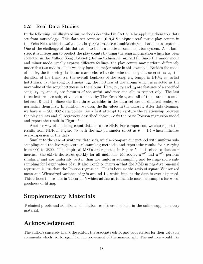
In the following, we illustrate our methods described in Section 4 by applying them to a dataset from musicology. This data set contains 1,019,318 unique users’ music play counts inthe Echo Nest which is available at http://labrosa.ee.columbia.edu/millionsong/tasteprofile.One of the challenge of this dataset is to build a music recommendation system. As a basicstep, it is interesting to predict the play counts by using the song information which has beencollected in the Million Song Dataset (Bertin-Mahieux et al., 2011). Since the major modeand minor mode usually express different feelings, the play counts may perform differentlyunder this two modes. Thus we only focus on major mode in this example. Besides the modeof music, the following six features are selected to describe the song characteristics: x1, theduration of the track; x2, the overall loudness of the song; x3, tempo in BPM; x4, artisthotttnesss; x5, the song hotttnesss; x6, the hottness of the album which is selected as themax value of the song hotttnesss in the album. Here, x1, x2 and x3 are features of a specifiedsong; x4, x5 and x6 are features of the artist, audience and album respectively. The lastthree features are subjective assessments by The Echo Nest, and all of them are on a scalebetween 0 and 1. Since the first three variables in the data set are on different scales, wenormalize them first. In addition, we drop the NA values in the dataset. After data cleaning,we have n = 205, 032 data points. As a first attempt to capture the relationship betweenthe play counts and all regressors described above, we fit the basic Poisson regression modeland report the result in Figure 5a.

Another way of modeling count data is to use NBR. For comparison, we also report theresults from NBR in Figure 5b with the size parameter select as θ = 1.4 which indicatesover-dispersion of the data.

Similar to the case of synthetic data sets, we also compare our method with uniform sub-sampling and the leverage score subsampling methods, and report the results for r varyingfrom 600 to 2800. The empirical MSEs are reported in Figure 5. It is clear to that as rincrease, the eMSE decreases quickly for all methods. Moreover, πmV and πmVc performsimilarly, and are uniformly better than the uniform subsampling and leverage score sub-sampling for larger values of r. It also worth to mention that the MSE in negative binomialregression is less than the Poisson regression. This is because the ratio of square Winsorizedmean and Winsorized variance of y is around 1.4 which implies the data is over-dispersed.This echoes the results in Theorem 5 which advise us to include more subsamples for worsegoodness of fitting.

Supplementary Materials

Technical proofs and additional simulation results are included in the online supplementarymaterial.

Acknowledgement

The authors sincerely thank the editor, the associate editor and two referees for their valuablecomments which led to significant improvement of the manuscript. The authors would like

18

0.0

2.5

5.0

7.5

1000 1500 2000

r

eMS

E

method

UNIF

mV

mVc

Lev

Lev−A

(a) Poisson Regression

0

1

2

3

4

5

1000 1500 2000

r

eMS

E

method

UNIF

mV

mVc

Lev

Lev−A

(b) Negative Binomial Regression

Figure 5: Empirical MSEs for different second step subsample size r with the first stepsubsample size being fixed at r0 = 400.

to thank Prof. Jinzhu Jia for his helpful suggestions and discussions. Ai’work is supportedby NNSF of China grants 11671019 and LMEQF. Wang’s work is partially supported byNSF grant 1812013 and an UConn REP grant.

A. Proofs

To prove Theorem 1, we begin with the following remark and lemma.

Remark 1. By the fact that λ(θ) : = exp(ψ(θ)) is analytic in the interior of Θ (see Theorem2.7 in Brown (1986)), Cauchy’s integral formula tells us that all its higher derivatives existand are continuous. Therefore, the derivatives ψ(t), ψ(t),

...ψ(t) are continuous in t, and

ψ(t),ψ(t) are bounded on the compact set, which follows by a well-known property thatevery real-valued continuous function on a compact set is necessarily bounded.

Lemma 1. If Assumptions (H.1)–(H.4) and (H.6) hold, then as r → ∞ and n → ∞,conditionally on Fn in probability,

JX − JX = OP |Fn(r−1/2), (12)

1

nL∗(β)− 1

nL(β) = OP |Fn(r−1/2), (13)

1

n

∂L∗(βMLE)

∂β= OP |Fn(r−1/2), (14)

where

JX = − 1

n

∂2L∗(βMLE)

∂β∂βT=

1

nr

r∑i=1

ψ(u(βTx∗i))u(βTx∗i)x∗i [u(βTMLEx

∗i )x

∗i ]T

π∗i

+1

nr

r∑i=1

u(βTMLEx∗i )x

∗ix∗Ti [ψ(u(βTMLEx

∗i ))− y∗i ]

π∗i.

19

Proof. By the definition of conditional expectation and towering property of flirtations, ityields that

E(JX |Fn) = JX .For any component J j1j2

X of JX where 1 ≤ j1, j2 ≤ p,

E(J j1j2X − J j1j2

X

∣∣∣Fn)2

(15)

=1

r

n∑i=1

πi

{ψ(u(βTMLExi))u

2(βTMLExi)xij1xij2nπi

+u(βTMLExi)xij1xij2 [ψ(u(βTMLExi))− yi]

nπi− J j1j2

X

}2

=1

r

n∑i=1

πi

{ψ(u(βTMLExi))u

2(βTMLExi)xij1xij2nπi

+u(βTMLExi)xij1xij2 [ψ(u(βTMLExi))− yi]

nπi

}2

− 1

r

(J j1j2X

)2

≤2

r

n∑i=1

πi

[{ψ(u(βTMLExi))u

2(βTMLExi)xij1xij2nπi

}2

+

{u(βTMLExi)xij1xij2 [ψ(u(βTMLExi))− yi]

nπi

}2 ]

≤2

r

n∑i=1

πi

[OP (1)

{xij1xij2nπi

}2

+OP (1)

{xij1xij2 [ψ(u(βTMLExi))− yi]

nπi

}2 ]=OP |Fn(

1

r)

where the last inequality stems form (H.1) and the last equality holds by assumptions (H.3)and (H.6). From Chebyshev’s inequality, it is proved that Equation (12) holds.

To prove Equation (14), let ti(β) = yiu(βTxi) − ψ(u(βTxi), t∗i (β) = y∗i u(βTx∗i ) −

ψ(u(βTx∗i )), then

L∗(β) =1

r

r∑i=1

t∗i (β)

π∗i, and L(β) =

n∑i=1

ti(β).

Under the conditional distribution of the subsample given Fn,

E

{L∗(β)

n− L(β)

n

∣∣∣∣Fn}2

=1

rn2

n∑i=1

t2i (β)

πi− 1

r

(1

n

n∑i=1

ti(β)

)2

.

Combining the facts that the parameter space is compact and u(t) is continuous function,by assumption (H.1) we have that u(βTxi) are uniformly bounded. Then, it can be shownthat by Remark 1

|ti(β)| ≤ |yiu(βTxi)− ψ(u(βTxi))u(βTxi)|+ |ψ(u(βTxi))u(βTxi)− ψ(u(βTxi))|≤ |[yi − ψ(u(βTxi))]u(βTxi)|+ |ψ(u(βTxi))u(βTxi)|+ |ψ(u(βTxi))|,

20

Therefore, we have(1

n

n∑i=1

ti(β)

)2

≤

(1

n

n∑i=1

OP (1)|yi − ψ(u(βTxi))|

)2

+OP (1)

n

n∑i=1

|yi − ψ(u(βTxi))|+OP (1).

From Assumptions (H.1), we have supnn−1

∑ni=1 ti(β) <∞. Thus,

E

{L∗(β)

n− L(β)

n

∣∣∣∣Fn}2

= OP |Fn(r−1/2). (16)

Now the desired result (13) follows from Chebyshev’s Inequality.Similarly, we can show that

Var

(1

n

∂L∗(βMLE)

∂β

)= OP (r−1).

Thus (14) is true.

A.1 Proof of Theorem 1

Proof. As r →∞, by (16), we have that n−1L∗(β)−n−1L(β)→ 0 in conditional probabilitygiven Fn. Note that the parameter space is compact and βMLE is the unique global maximumof the continuous convex function L(β). Thus, from Theorem 5.9 and its remark of van derVaart (1998), by (14) we have

‖β − βMLE‖ = oP |Fn(1). (17)

as n→∞, r →∞, conditionally on Fn in probability.Using Taylor’s theorem for random variables (see Ferguson, 1996, Chapter 4),

0 =L∗j(β)

n=L∗j(βMLE)

n+

1

n

∂L∗j(βMLE)

∂βT(β − βMLE) +

1

nRj, (18)

where L∗j(β) is the partial derivative of L∗(β) with respect to βj, and the remainder

1

nRj =

1

n(β − βMLE)T

∫ 1

0

∫ 1

0

∂2L∗j{βMLE + uv(β − βMLE)}∂β∂βT

vdudv (β − βMLE).

By calculus, we get

∂2L∗j(β)

∂β∂βT=

1

r

r∑i=1

{...u (βTx∗i )[y

∗i − ψ(u(βTx∗i ))]

π∗i− u(βTx∗i )u(βTx∗i )ψ(u(βTx∗i ))

π∗i

21

− 2ψ(u(βTx∗i ))u(βTx∗i )u(βTx∗i )

π∗i−

...ψ(u(βTx∗i ))u

2(βTx∗i )

π∗i}x∗ijx∗ix∗i

T .

From (H.1) and Remark 1, we have

1

n

∥∥∥∥∥∂2L∗j(β)

∂β∂βT

∥∥∥∥∥S

=1

nr

∥∥∥∥ r∑i=1

(u(βTx∗i )ψ(u(βTx∗i ))

π∗i+

2ψ(u(βTx∗i ))u(βTx∗i )

π∗i+

...ψ(u(βTx∗i ))u(βTx∗i )

π∗i

)u(βTx∗i )x

∗ijx∗ix∗iT

∥∥∥∥S

+1

rn

∥∥∥∥∥r∑i=1

...u (βTx∗i )[y

∗i − ψ(u(βTx∗i ))]

π∗i

∥∥∥∥∥S

≤C3

rn

r∑i=1

‖x∗i ‖3

π∗i+C4

rn

∥∥∥∥∥r∑i=1

|[y∗i − ψ(u(βTx∗i )]x∗ij|

π∗ix∗ix

∗iT

∥∥∥∥∥S

.

for all β ∈ ΛB, where C3 and C4 are some constants by using Remark 1.As τ →∞, assumption (H.5) gives,

P

(1

nr

r∑i=1

‖x∗i ‖3

π∗i≥ τ

∣∣∣∣∣Fn)≤ 1

nrτ

r∑i=1

E

(‖x∗i ‖3

π∗i

∣∣∣∣∣Fn)

=1

nτ

n∑i=1

‖xi‖3 P→ 0.

Also note that as τ →∞,

P

(1

nr

r∑i=1

∥∥∥∥∥ |[yi − ψ(u(βTxi))]xij|xixTiπ∗i

∥∥∥∥∥S

≥ τ∣∣∣Fn)

≤ 1

nrτE

(r∑i=1

∥∥∥∥∥ |[yi − ψ(u(βTxi))]xij|xixTiπ∗i

∥∥∥∥∥S

∣∣∣Fn)

≤ 1

nτ

n∑i=1

∥∥∥|[yi − ψ(u(βTxi))]xij|xixTi∥∥∥S

≤ 1

τn

n∑i=1

|[yi − ψ(u(βTxi))]| ×∥∥xijxixTi ∥∥S

≤ 1

τ

√√√√ 1

n

n∑i=1

|yi − ψ(u(βTxi))|2 ·

√√√√ 1

n

n∑i=1

‖xijxixTi ‖2

S

=1

τOP (1)

P→ 0,

where the last equality is due to (H.3) and (H.5) by noticing that

1

n

n∑i=1

∥∥x∗ijx∗ix∗Ti ∥∥2

S≤ 1

n

n∑i=1

∣∣x∗ij∣∣2 ∥∥x∗ix∗Ti ∥∥2

S

22

≤ 1

n

n∑i=1

‖xi‖2∥∥xixTi ∥∥2

S≤ 1

n

n∑i=1

‖xi‖6.

Thus we have1

n

∥∥∥∥∥∂2L∗j(β)

∂β∂βT

∥∥∥∥∥S

= OP |Fn(1).

From (H.1)-(H.3) and Remark 1, it is known that

1

n

∥∥∥∥∥∫ 1

0

∫ 1

0

∂2L∗j{βMLE + uv(β − βMLE)}∂β∂βT

vdudv

∥∥∥∥∥≤ 1

n

∫ 1

0

∫ 1

0

∥∥∥∥∥∂2L∗j{βMLE + uv(β − βMLE)}∂β∂βT

∥∥∥∥∥ vdudv = OP |Fn(1).

Combining the above equations with the Taylor’s expansion (18), we have

β − βMLE = −J −1X

{L∗(βMLE)

n+OP |Fn(‖β − βMLE‖2)

}. (19)

From Lemma 1 and Assumption (H.4), it is obvious that J −1X = OP |Fn(1). Therefore,

β − βMLE = OP |Fn(r−1/2) + oP |Fn(‖β − βMLE‖),

which implies that β − βMLE = OP |Fn(r−1/2).

A.2 Proof of Theorem 2

Proof. Note that

L∗(βMLE)

n=

1

r

r∑i=1

{y∗i − ψ(u(βTMLEx∗i ))}u(βTMLEx

∗i )x

∗i

nπ∗i=:

1

r

r∑i=1

ηi. (20)

It can be seen that given Fn, η1, . . . , ηr are i.i.d random variables with mean 0 and variance

var(η1|Fn) =1

n2

n∑i=1

{yi − ψi(u(βTMLExi))}2u2(βTMLExi)xixTi

πi. (21)

Then from (H.7) with γ = 0, we know that var(ηi|Fn) = OP (1) as n→∞.Meanwhile, for some γ > 0 and every ε > 0,

r∑i=1

E{‖r−1/2ηi‖2I(‖ηi‖ > r1/2ε)|Fn}

≤ 1

r1+γ/2εγ

r∑i=1

E{‖ηi‖2+γI(‖ηi‖ > r1/2ε)|Fn}

≤ 1

r1+γ/2εγ

r∑i=1

E(‖ηi‖2+γ|Fn)

=1

rγ/21

εγ1

n2+γ

n∑i=1

|yi − ψi(u(βTMLExi))|2+γ‖u(βTMLExi)xi‖2+γ

π1+γi

.

(22)

23

From (H.7) for some γ > 0, we obtain

r∑i=1

E{‖r−1/2ηi‖2I(‖ηi‖ > r1/2ε)|Fn} ≤1

rγ/21

εγOP (1) ·OP (1) = oP (1),

This shows that the Lindeberg-Feller conditions are satisfied in probability. From (20) and(21), by the Lindeberg-Feller central limit theorem (Proposition 2.27 of van der Vaart, 1998),conditionally on Fn,

1

nV −1/2c L∗(βMLE) =

1

r1/2{var(ηi|Fn)}−1/2

r∑i=1

ηi → N(0, I),

in distribution. From Lemma 1, (19) and Theorem 1, we have

β − βMLE = − 1

nJ −1X L∗(βMLE) +OP |Fn(r−1). (23)

From (12) in Lemma 1, it follows that

J −1X − J

−1X = −J −1

X (JX − JX)J −1X = OP |Fn(r−1/2). (24)

Based on Assumption (H.4) and (21), it can be proved that

V = J −1X VcJ −1

X =1

rJ −1X (rVc)J −1

X = OP (r−1).

Thus,

V −1/2(β − βMLE) = −V −1/2n−1J −1X L∗(βMLE) +OP |Fn(r−1/2)

=− V −1/2J −1X n−1L∗(βMLE)− V −1/2(J −1

X − J−1X )n−1L∗(βMLE) +OP |Fn(r−1/2)

=− V −1/2J −1X V 1/2

c V −1/2c n−1L∗(βMLE) +OP |Fn(r−1/2).

So the result in (4) of Theorem 2 follows by applying Slutsky’s Theorem (Theorem 6, Section6 of Ferguson, 1996) and the fact that

V −1/2J −1X V 1/2

c (V −1/2J −1X V 1/2

c )T = V −1/2J −1X V 1/2

c V 1/2c J −1

X V −1/2 = I.

A.3 Proof of Theorem 3

Proof. Note that

tr(V ) = tr(J −1X VcJ −1

X )

=1

n2r

n∑i=1

tr

[1

πi{yi − ψ(u(βTMLExi))}2J −1

X u(βTMLExi)xi[u(βTMLExi)xi]TJ −1

X

]

24

=1

n2r

n∑i=1

[1

πi{yi − ψ(u(βTMLExi))}2‖J −1

X u(βTMLExi)xi‖2

]=

1

n2r(n∑i=1

πi)n∑i=1

[π−1i {yi − ψ(u(βTMLExi))}2‖J −1

X u(βTxi)xi‖2]

≥ 1

n2r

[n∑i=1

|yi − ψ(u(βTMLExi))|‖J −1X u(βTMLExi)xi‖

]2

,

where the last inequality follows from the Cauchy-Schwarz inequality, and the equality in itholds if and only if

πi ∝ |yi − ψ(u(βTMLExi))|‖J −1X xi‖I{|yi − ψ(u(βTMLExi))|‖J −1

X xi‖ > 0}.

Here we define 0/0 = 0, and this is equivalent to removing data points with |yi−ψ(u(βTMLExi))| =0 in the expression of Vc.

A.4 Proof of Theorems 5 and 6

Let ‖A‖F := (∑m

i=1

∑nj=1 A

2ij)

1/2 denote the Frobenius norm. For a given m×n matrix A andan n×p matrix B, we want to get an approximation to the product AB. In the following fastMonte Carlo algorithm in Drineas et al. (2006a), we do r independent trials. In each trial werandomly sample an element of {1, 2, · · · , n} with given discrete distribution P =: {pi}ni=1.Then we extract an m× r matrix C from the columns of A, and extract an r × n matrix Rfrom the corresponding rows of B. If the P is chosen appropriately in the sense that CR isa nice approximation to AB, then the F-norm matrix concentration inequality in Lemma 2holds with high probability.

Lemma 2. (Theorem 2.1 in Drineas et al. (2006b)) Let A(i) be the i-th row of A ∈ Rm×n

as row vector and B(j) be the j-th column of B ∈ Rn×p as column vector. Suppose samplingprobabilities {pi}ni=1, (

∑ni=1 pi = 1) are such that

pi ≥ β

∥∥A(i)∥∥∥∥B(j)

∥∥∑nj=1 ‖A(i)‖

∥∥B(j)

∥∥for some β ∈ (0, 1]. Construct C and R with Algorithm 1 in Drineas et al. (2006a), andassume that ε ∈ (0, 1/3). Then, with probability at least 1− ε, we have

‖AB − CR‖F ≤4√

log(1/ε)

β√c

‖A‖F‖B‖F .

Now we prove Theorems 5 and 6 by applying the above Lemma 2.

Proof. Note the fact that the maximum likelihood estimate βMLE of the parameter vector βsatisfy the following estimation equation

XT [y − ψ(u(XTβ))]u(XTβ) = 0, (25)

25

where ψ(u(XTβ)) denotes the n × n diagonal matrix whose i-th element in its diagonal isψ(u(xTi β)).

Without of loss of generality, we only show the case with probability πmV, since the

proof for πmVc is quite similar. Let S be an n× r matrix whose i-th column is 1/√rπmV

jieji ,

where eji ∈ Rn denotes the all-zeros vector except that its ji-th entry is set to one. Hereji denotes the ji-th data point chosen from the i-th independent random subsampling withprobabilities πmV. Then β satisfies the following equation

XTSST [y − ψ(u(XTβ))]u(XTβ) = 0. (26)

Let ‖ · ‖F denote the Frobenius norm, we have

σmin(XTSST u(XT β))‖[ψ(u(XT β))− ψ(u(XT βMLE))]‖≤ ‖XTSST u(XT β)[ψ(u(XT β))− ψ(u(XT βMLE))]‖F≤ ‖XTSST u(XT β)[ψ(u(XT β))− y]‖F+ ‖XTSST u(XT β)[y − ψ(u(XT βMLE))]‖F= ‖XTSST u(XT β)[y − ψ(u(XT βMLE))]‖F [by (26)]

≤ ‖XT u(XT β)[y − ψ(u(XT βMLE))]‖F+∥∥∥XT u(XT β)[y − ψ(u(XT βMLE))]−XTSST u(XT β)[y − ψ(u(XT βMLE))]

∥∥∥F

≤ ‖XT u(XT β)[y − ψ(u(XT βMLE))]‖F

+4κ(J −1

X )√

log(1/ε)√r

‖X‖F‖u(XT β)[y − ψ(u(XT βMLE))]‖

≤ σmax(X)√p‖u(XT β)[y − ψ(u(XT βMLE))]‖

+4κ(J −1

X )√

log(1/ε)√r

σmax(X)√p‖u(XT β)[y − ψ(u(XT βMLE))]‖

≤ [1 +4κ(J −1

X )√

log(1/ε)√r

]σmax(X)√p‖u(XT β)[y − ψ(u(XT βMLE))]‖

≤ Cu[1 +4κ(J −1

X )√

log(1/ε)√r

]σmax(X)√p‖[y − ψ(u(XT βMLE))]‖

where the fourth last inequality follows from Lemma 2 by putting A = XT u(XT β), B =u(XT β)[y − ψ(u(XT βMLE))], C = XTS, R = ST u(XT β)(y − ψ(u(XT βMLE))) and β =1/κ(J −1

X ), and last equality stems from (H.1) and Remark 1 with Cu = supr∈K⊂Θ

|u(r)|.

Hence,

‖ψ(u(XT βMLE))− ψ(u(XT β))‖

≤Cu[1 +

4κ(J−1X )√

log(1/ε)√r

]√pσmax(X)

σmin(u(XT β)XTSST )‖[y − ψ(u(XT βMLE))]‖. (27)

26

Then by following the facts that

σmin(u(XT β)XTSSTXu(XT β)) ≤ σmax(u(XT β)X)σmin(u(XT β)XTSST )

and σ2min(u(XT β)XT ) = σmin(u(XT β)XTSSTXu(XT β)) ≥ 0.5σ2

min(X), it holds that

σmin(u2(XT β)XTSST ) ≥ 0.5σ2min(u(XT β)X)/σmax(u(XT β)X). (28)

Combing the result (28) with (27), the desired result holds

‖ψ(u(XT βMLE))− ψ(u(XT β))‖

≤ 2Cu[1 +4α√

log(1/ε)√r

]√pκ2(u(XT β)X)‖[y − ψ(u(XT βMLE))]‖. (29)

Now, we turn to prove Theorem 6.Note that

pi ≥ αminj |yj − ψ(u(βTMLExj))||u(βTMLExj)|√∑

j |yj − ψ(u(βTMLExj))|2|u2(βTMLExj)|

‖xi‖∑j ‖xj‖

= δ‖xi‖∑j ‖xj‖

,

with some 0 < δ := αγ√∑j |yj−ψ(u(βTMLExj))|2|u2(βTMLExj)|

≤ 1.

According to the Weyl inequality, we have

|σmin(u(XT β)XT u(XT β)X)− σmin(u(XT β)XTSSTXu(XT β))|≤‖u(XT β)XT u(XT β)X − u(XT β)XTSSTXu(XT β)‖S≤‖u(XT β)‖S‖(XTX −XTSSTX)‖S‖u(XT β)‖S≤cdC2

u‖(XTX −XTSSTX)‖F

≤cd4√

log(1/ε)C2u

δ√r

‖X‖2F

≤cd4√

log(1/ε)C2u

δ√r

pσ2max(X).

Using the above inequality, if we set

r > 64c2dC

2u log(1/ε)σ4

max(X)p2/(δ2σ4min(u(XT β)X)),

it holds that

|σmin(u(XT β)XTSSTXu(XT β))− σmin(u(XT β)XTXu(XT β))|≤0.5σmin(u(XT β)XTXu(XT β)).

Thus the following equation holds with probability at least 1− ε:

σmin(u(XT β)XTSSTXu(XT β)) ≥ 0.5σ2min(u(XT β)X).

27

A.5 Proof of Theorem 7

For the average weighted log-likelihood in Step 2 of two-step algorithm, we have

Ltwo−step

β0(β) : =

1

r + r0

r+r0∑i=1

t∗i (β)

π∗i (β0)=

1

r + r0

[

r0∑i=1

t∗i (β)

π∗i (β0)+

r+r0∑i=r0+1

t∗i (β)

π∗i (β0)]

=r0

r + r0

· 1

r0

r0∑i=1

t∗i (β)

π∗i (β0)+

r

r + r0

· 1

r

r+r0∑i=r0+1

t∗i (β)

π∗i (β0),

where π∗i (β0) in the first item stands for the initial subsampling strategy which satisfies(H.5).

For the sake of brevity, we begin with the case with probability πmV. Denote the log-likelihood in the first and second steps by

L∗0β0

(β) =1

r0

r0∑i=1

t∗i (β)

π∗i (β0), and L∗

β0(β) =

1

r

r∑i=1

t∗i (β)

π∗i (β0),

respectively, where πi(β0) = πopti in L∗

β0(β), and it has been calculated in the two-step

algorithm in Section 4.To proof of Theorem 7, we begin with the following Lemma 3.

Lemma 3. If Assumptions (H.1)–(H.4) holds, then as n → ∞, conditionally on Fn inprobability,

J β0

X − JX = OP |Fn(r−1/2), (30)

1

n

∂L∗β0

(βMLE)

∂β= OP |Fn(r−1/2), (31)

where

J β0

X = − 1

n

∂2L∗β0

(βMLE)

∂β∂βT=

1

nr

r∑i=1

ψ(u(βTx∗i))u(βTx∗i)x∗i [u(βTMLEx

∗i )x

∗i ]T

π∗i (β0)

+1

nr

r∑i=1

u(βTMLEx∗i )x

∗ix∗Ti [ψ(u(βTMLEx

∗i ))− y∗i ]

π∗i (β0).

Proof. Using the same arguments in Lemma 1, we have

E(J β0,j1j2X − J j1j2

X

∣∣∣Fn, β0

)2

≤ OP (1)

r

[ n∑i=1

u2(βTMLExi)(xij1xij2)2

n2πi(β0)

+n∑i=1

{u2(βTMLExi)xij1xij2 [ψ(u(βTMLExi))− yi]}2

n2πi(β0)

].

(32)

Now we substitute expression of πi(β0) in the two-step algorithm: πmV and πmVc. Herewe only give the proof of the case πmV, and the proof of the case πmVc is analogous thus

28

we omit it. For the first terms in (32), note that σmax(J −1X ), σmin(J −1

X ) are bounded fromLemma 1 and (H.4), it implies

n∑i=1

u2(βTMLExi)(xij1xij2)2

n2πi(β0)

≤n∑i=1

∥∥∥u2(βTMLExi)xi

∥∥∥2 n∑j=1

max(|yj − ψ(u(βT0 xj))|, δ)∥∥∥J −1

X u(βT0 xi)xi

∥∥∥n2 max(|yj − ψ(u(βT0 xj))|, δ)

∥∥∥J −1X u(βT0 xi)xi

∥∥∥≤

n∑i=1

∥∥∥u2(βTMLExi)xi

∥∥∥2 n∑j=1

max(|yj − ψ(u(βT0 xj))|, δ)σmax(J −1X )

∥∥∥u2(βT0 xi)xi

∥∥∥n2δσmin(J −1

X )∥∥∥u2(βT0 xi)xi

∥∥∥≤ κ(J −1

X )n∑i=1

‖u2(βTMLExi)xi‖n2δ

[ n∑j=1

|yj − ψ(u(βT0 xj))|‖u2(βT0 xi)xj‖n

+n∑j=1

δ‖u2(βT0 xi)xj‖n

]

≤ κ(J −1X )

n∑i=1

‖u2(βTMLExi)xi‖nδ

[√√√√ n∑j=1

|yj − ψ(u(βT0 xj))|2n

√√√√ n∑j=1

‖u2(βT0 xi)xj‖2

n

+n∑j=1

δ‖u2(βT0 xi)xj‖n

]

≤ OP (1)κ(J −1X )

n∑i=1

‖xi‖nδ

√√√√ n∑j=1

|yj − ψ(u(βT0 xj))|2n

√√√√ n∑j=1

‖xj‖2

n+

n∑j=1

δ‖xj‖n

= OP (1).

where the last equality is from (H.3) and (H.5).For the second terms in (32), we have

n∑i=1

(u2(βTMLExi)xij1xij2 [ψ(u(βTMLExi))− yi])2

n2πi(β0)

≤n∑i=1

∥∥∥u2(βTMLExi)xi

∥∥∥2∣∣∣ψ(u(βTMLExi))− yi∣∣∣2

n2δ∥∥∥J −1

X u(βT0 xi)xi

∥∥∥×

n∑j=1

(|yj − ψ(u(βT0 xj))|+δ)∥∥∥J −1

X u(βT0 xj)xj

∥∥∥≤ κ(J −1

X )n∑i=1

[∥∥∥u2(βTMLExi)xi

∥∥∥ ∣∣∣ψ(u(βTMLExi))− yi∣∣∣2

nδ

29

×

n∑j=1

(|yj − ψ(u(βT0 xj))|+δ)∥∥∥u(βT0 xj)xj

∥∥∥n

]

= κ(J −1X )

n∑i=1

∥∥∥u2(βTMLExi)xi

∥∥∥ ∣∣∣ψ(u(βTMLExi))− yi∣∣∣2

nδOP (1)

≤ κ(J −1X )

δ

√√√√√ n∑i=1

∥∥∥u2(βTMLExi)xi

∥∥∥2

n

√√√√√ n∑i=1

∣∣∣ψ(u(βTMLExi))− yi∣∣∣4

nOP (1)

= OP (1)

where the second last and last equality is from (H.3) and (H.5).Direct calculation yields

E(J β0,j1j2X − J j1j2

X |Fn)2

= Eβ0E(J β0,j1j2X − J j1j2

X |Fn, β0

)2

= OP (r−1)

where Eβ0means that the expectation is taken with respect to the distribution of β0 given

Fn.On the other hand, following the same arguments in Lemma 1, we can have

E

{L∗β0

(β)

n− L(β)

n

∣∣∣∣Fn, β0

}2

= OP (r−1).

Then E{n−1L∗

β0(β)− n−1L(β)|Fn

}2

= OP (r−1).

Similarly, we can see that Var(n−1∂L∗β0

(βMLE)/∂β) = OP (r−1). Thus, the desired result

holds.

Now we prove Theorem 7.

Proof. Using the same arguments in Lemma 3 , we have

E

{Ltwo−step

β0(β)

n− L(β)

n

∣∣∣∣Fn}2

≤ 2(r0

r + r0

)2E

{L∗0β0

(β)

n− L(β)

n

∣∣∣∣Fn}2

+ 2(r

r + r0

)2E

{L∗β0

(β)

n− L(β)

n

∣∣∣∣Fn}2

= OP (r−1).

Therefore E{n−1Ltwo−step

β0(β)−n−1L(β)|Fn}2 → 0 as r0/r → 0, r →∞ and n−1Ltwo−step

β0(β)−

n−1L(β) → 0 in conditional probability given Fn. Also note that the parameter space iscompact and βMLE is the unique global maximum of the continuous convex function L(β).Thus, from Theorem 5.9 and its remark of van der Vaart (1998), we have

‖β − βMLE‖ = oP |Fn(1).

30

Using Taylor’s theorem,

0 =Ltwo−step

β0,j(β)

n=

r0

r + r0

L∗0β0,j

(β)

n+

r

r + r0

L∗β0,j

(β)

n

=r

r + r0

{L∗β0,j

(βMLE)

n+

1

n

∂L∗β0,j

(βMLE)

∂βT(β − βMLE) +

1

nRβ0,j

}

+r0

r + r0

L∗0β0,j

(β)

n,

where L∗β0,j

(β) is the partial derivative of L∗β0,j

(β) with respect to βj.

By similar argument in the Proof of Theorem 1, the Lagrange remainder have the rate

1

nRβ0,j

:=1

n(β − βMLE)T

∫ 1

0

∫ 1

0

∂2L∗j{βMLE + uv(β − βMLE)}∂β∂βT

vdudv (β − βMLE)

= OP |Fn(‖β − βMLE‖2).

Note that the subsampling probabilities in the first stage satisfies the condition (H.1)-(H.7),thus from Theorem 2, it holds that

L∗0β0,j

(β)

n=L∗0β0,j

(βMLE)

n+

1

n

∂L∗0β0,j

(βMLE)

∂βT(β − βMLE) +OP |Fn(‖β − βMLE‖2).

Therefore

1

n

∂L∗0β0

(β)

∂β=

1

n

∂L∗0β0

(βMLE)

∂β+

1

n

∂2L∗0β0

(βMLE)

∂β∂βT(β − βMLE) +OP |Fn(‖β − βMLE‖2).

From Lemma 1, it is clear to see that

1

n

∂L∗0β0

(βMLE)

∂β= OP |Fn(r

−1/20 )

for the first step, since π∗i is prespecified and satisfied (H.6), and

r0

r + r0

1

n

∂L∗0β0

(βMLE)

∂β=r0

rOP |Fn(r

−1/20 ) = oP |Fn(r−1/2),

since r0/r → 0. This step holds due to the fact that√r0rOP |Fn(1) =

√r0√rOP |Fn(1)OP |Fn(r−1/2) =

o(1)OP |Fn(r−1/2). Let

JX :=r

r + r0

1

n

∂2L∗β0

(βMLE)

∂β∂βT+

r0

r + r0

1

n

∂2L∗0β0

(βMLE)

∂β∂βT.

31

Combine Lemmas 1 and 3, we have

JX − JX =r

r + r0

(J β0

X − JX)

+r0

r + r0

(1

n

∂2L∗0β0

(βMLE)

∂β∂βT− JX

)=

r

r + r0

OP |Fn(r−1/2) +r0

r + r0

OP |Fn(r−1/20 ) = OP |Fn(r−1/2),

since r0/r → 0.Hence,

β − βMLE =− (JX)−1

{1

nL∗β0

(βMLE) +OP |Fn(‖β − βMLE‖2) + oP |Fn(r−1/2)

},

=OP |Fn(r−1/2) + oP |Fn(‖β − βMLE‖)

as r0/r → 0, by noting (JX)−1 = OP |Fn(1) from (H.5). Therefore, the desired result followsby noting

β − βMLE = OP |Fn(r−1/2).

A.6 Proof of Theorem 8

Proof. For the sake of brevity, we begin with the case with probability πmVc. Denote

L∗β0

(βMLE)

n=

1

r

r∑i=1

{y∗i − ψ(u(βTMLEx∗i ))}u(βTMLEx

∗i )x

∗i

nπ∗i (β0)=:

1

r

r∑i=1

ηβ0

i . (33)

It can be shown that given Fn and β0, ηβ0

1 , . . . , ηβ0r are i.i.d random variables with zero mean

and variance

var(ηβ0

i |Fn, β0) = rV β0c =

1

n2

n∑i=1

πi(β0){y∗i − ψ(u(βTMLEx

∗i ))}2u2(βTMLEx

∗i )xix

Ti

π2i (β0)

.

Meanwhile, for every ε > 0,

r∑i=1

E{‖r−1/2ηβ0

i ‖2I(‖ηβ0

i ‖ > r1/2ε)|Fn, β0}

≤ 1

r3/2ε

r∑i=1

E{‖ηβ0

i ‖3I(‖ηβ0

i ‖ > r1/2ε)|Fn, β0}

≤ 1

r3/2ε

r∑i=1

E(‖ηβ0

i ‖3|Fn, β0)

≤ 1

r1/2

1

n3

n∑i=1

{|yi − ψ(u(βTMLExi))|}3‖u(βTMLExi)xi‖3

π2i (β0)

32

≤ 1

r1/2

1

n

n∑i=1

{|yi − ψ(u(βTMLExi))|}2‖u(βTMLExi)xi‖δ

×

(1

n

n∑j=1

max(|yj − ψ(u(βT0 xj))|, δ)‖u(βT0 xj)xj‖

)2

≤ 1

r1/2

1

n

n∑i=1

{|yi − ψ(u(βTMLExi))|}2‖u(βTMLExi)xi‖δ

×

(1

n

n∑j=1

(|yj − ψ(u(βT0 xj))|+ δ)‖u(βT0 xj)xj‖

)2

.

From (H.1), (H.3) and (H.5),

1

n

n∑i=1

{|yi − ψ(u(βTMLExi))|}2‖u(βTMLExi)xi‖δ

≤δ−1

(1

n

n∑i=1

{|yi − ψ(u(βTMLExi))|}4

)1/2(1

n

n∑i=1

‖u(βTMLExi)xi‖2

)1/2

=OP (1),

by Holder’s inequality.Similarly, it can be shown

1

n

n∑j=1

(|yj − ψ(u(βT0 xj))|+ δ)‖u(βT0 xj)xj‖ = OP (1),

from (H.1), (H.3) and (H.5).Hence

r∑i=1

E{‖r−1/2ηβ0

i ‖2I(‖ηβ0

i ‖ > r1/2ε)|Fn, β0} = oP |Fn(1).

This shows that the Lindeberg-Feller conditions are satisfied in probability. By the Lindeberg-Feller central limit theorem (Proposition 2.27 of van der Vaart, 1998), conditionally on Fnand β0,

1

n(V β0

c )−1/2L∗(βMLE) =1

r1/2{var(ηi|Fn, β0)}−1/2

r∑i=1

ηi → N(0, I),

in distribution.The distance between V β0

c and Vc is

‖Vc − V β0c ‖

≤ 1

r

n∑i=1

∥∥∥∥ 1

πmVci

− 1

πi(β0)

∥∥∥∥ {yi − ψ(u(βTMLExi))}2u2(βTMLExi)‖xi‖2

n

=1

r

n∑i=1

∥∥∥∥1− πmVci

πi(β0)

∥∥∥∥ {yi − ψ(u(βTMLExi))}2u2(βTMLExi)‖xi‖2

nπmVci

33

≤ 1

r

n∑i=1

∥∥∥∥1− πmVci

πi(β0)

∥∥∥∥ |yi − ψ(u(βTMLExi))|‖u(βTMLExi)xi‖n

≤ 1

r

(1

n

n∑i=1

∥∥∥∥1− πmVci

πi(β0)

∥∥∥∥2)1/2( n∑

i=1

{yi − ψ(u(βTMLExi))}2u2(βTMLExi)‖xi‖2

n

)1/2

= oP |Fn(r−1),

where the last equation follows from the facts that∥∥∥∥1− πmVci

πi(β0)

∥∥∥∥2

≤ (πmVci − πi(β0))2

δ2= oP (1),

andn∑i=1

{yi − ψ(u(βTMLExi))}2u2(βTMLExi)‖xi‖2

n= OP (1).

Here the first equality in the fact above holds for the continues mapping theorem and thesecond equality holds from (H.1), (H.3), (H.5) and Cauchy’s inequality.

Utilizing the facts

(J β0

X )−1 − J −1X = −J −1

X (J β0

X − JX + JX − JX)(J β0

X )−1 = OP |Fn(r−1/2),

we have (J β0

X )−1 − (JX)−1 = OP |Fn(r−1/2) from Lemma 3 and Theorem 7. Thus

β − βMLE=− 1

n(J β0

X )−1L∗β0

(βMLE) +OP |Fn(r−1) (34)

Based on Equation (30), we further have

(J β0

X )−1 − J −1X = −J −1

X (J β0

X − JX)(J β0

X )−1 = OP |Fn(r−1/2).

Therefore

V −1/2(β − βMLE)

=− V −1/2 1

n(J β0

X )−1L∗(βMLE) +OP |Fn(r−1/2)

=− V −1/2J −1X

1

nL∗(βMLE)− V −1/2{(J β0

X )−1 − J −1X }

1

nL∗(βMLE) +OP |Fn(r−1/2)

=− V −1/2J −1X (V β0

c )1/2(V β0c )−1/2 1

nL∗(βMLE) +OP |Fn(r−1/2).

It can be shown that

V −1/2J −1X (V β0

c )1/2(V −1/2J −1X (V β0

c )1/2)T

=V −1/2J −1X (V β0

c )J −1X V −1/2

=V −1/2J −1X (Vc)J −1

X V −1/2 + oP |Fn(r−1/2)

=I + oP |Fn(r−1/2).

The desired result follows by Slutsky’s theorem.As for the case πi(β0) = πmV

i in L∗β0

(β), πmVi has the same expression as πmV

i except that

βMLE, is replaced by β0. Also note that πi(β0) ≥ κ(JX)−1πmVci . The rest of the proof is the

same as that of πmVci with minor modifications.

34

B. Additional Simulation Results

In terms of the allocation between r0 and r, it is clear to see that the two-step approach worksthe best when r0/r is around 0.2 from the simulation result in Figure 3 of the main text. Towell demonstrate our methods, we also compare different r0 + r with fixed r0/r = 0.2.

In each of the settings described in Section 5.1 of the article, we reevaluated the perfor-mance of πmV

i and πmVci when r0/r is fixed at 0.2. For comparison, the uniform subsampling,

leverage subsampling and adjust leverage subsampling methods are also considered. Inlinewith the setting in the main text, the sample size r0 + r is selected as 500, 700, 900, 1200,1400 and 1600, respectively. We report the results for the Poisson regression and negativebinomial regression in Figures 6 and 7, respectively.

0.000

0.005

0.010

0.015

0.020

0.025

800 1200 1600r0+r

eMS

E

method

UNIF

mV

mVc

Lev

Lev−A

(a) Case 1

0.0

0.2

0.4

0.6

800 1200 1600r0+r

eMS

E

method

UNIF

mV

mVc

Lev

Lev−A

(b) Case 2

0.000

0.005

0.010

0.015

0.020

800 1200 1600r0+r

eMS

E

method

UNIF

mV

mVc

Lev

Lev−A

(c) Case 3

0.00

0.01

0.02

800 1200 1600r0+r

eMS

E

method

UNIF

mV

mVc

Lev

Lev−A

(d) Case 4

Figure 6: The eMSEs for Poisson regression with different subsample size r0 + r and a fixedr0/r = 0.2. The different distributions of covariates are listed in the beginning of Section 5.

From Figures 6 and 7, we can see that our methods are slightly better than the casesthat r0 is fixed at 200. However, this improvement is not significant.

To explore influential factors on subsample sizes that have been discussed in Section 3.2in terms of estimation accuracy, we consider additional four cases for the Poisson regressionmodels listed as below.

Case S1: The true value of β is a 7×1 vector of 0.5 and the covariates matrix X = Σ−1/2n X.

Here X is the centralized version of a n × 7 matrix whose elements are i.i.d.,generated from U([−1, 1]), and Σn is the sample covariance matrix of X so that Xhas a sample covariance matrix as Ip and a condition number as 1.

Case S2: The true value of β is a 14 × 1 vector whose first seven elements are set to be0.5 and rest are set to be 0.1. The covariates matrix X = Σ

−1/2n X, where X is

35

0.000

0.025

0.050

0.075

0.100

800 1200 1600r0+r

eMS

E

method

UNIF

mV

mVc

Lev

Lev−A

(a) Case 1

0

1

2

3

800 1200 1600r0+r

eMS

E

method

UNIF

mV

mVc

Lev

Lev−A

(b) Case 2

0.00

0.03

0.06

0.09

800 1200 1600r0+r

eMS

E

method

UNIF

mV

mVc

Lev

Lev−A

(c) Case 3

0.00

0.03

0.06

0.09

800 1200 1600r0+r

eMS

E

method

UNIF

mV

mVc

Lev

Lev−A

(d) Case 4

Figure 7: The eMSEs for NBR with different subsample size r0 + r and a fixed r0/r = 0.2.The different distributions of covariates are listed in the beginning of Section 5.

the centralized version of a n × 14 matrix whose elements are i.i.d. generatedfrom U([−1, 1]) and Σn is the sample covariance matrix of X so that the conditionnumber of X is 1 and the signal to noise ratio is nearly the same as that in CaseS1.

Case S3: This case is the same as the Case S2 except that we replace xi2 in Case S2 with

xi2 = xi1 + εi where εii.i.d∼ U([−0.4, 0.4]) for i = 1, . . . , n. For this setup, the

condition number of X is around 5.

Case S4: This case is the same as the Case S2 except that we replace xi2 in Case S2 with

xi2 = xi1 + εi where εii.i.d∼ U([−0.1, 0.1]) for i = 1, . . . , n. For this setup, the

condition number of X is around 26.

To exclude the pilot subsampling effect, the ideal case that βMLE is given before conductingthe subsampling strategy is considered. Although this setting is hard to satisfy, the sim-ulation provides some key insights for Theorem 5 and it is also valuable for the two stepAlgorithm. The sample size r is selected as 10, 15, 20, 25 and 30 times of the dimensionrespectively. For comparison, the uniform subsampling method is also demonstrated. Theempirical MSEs are reported in Figures 8.

Through the simulation results reported in Figures S3(a) and S3(b), we can see thatthe cases with r = 10p, 20p have similar performance when the conditional numbers of thecovariate matrix are fixed at one. And for the same dimensional case, the eMSEs becomelarger as the conditional number of the covariate matrix increasing. These echo the resultsdiscussed in Section 3.2.

36

0.00

0.02

0.04

0.06

10 15 20 25 30c

eMS

E

method

UNIF

mV

mVc

(a) Case S1 (p = 7, κ = 1)

0.00

0.02

0.04

0.06

10 15 20 25 30c

eMS

E

method

UNIF

mV

mVc

(b) Case S2 (p = 14, κ = 1)

0.00

0.05

0.10

0.15

10 15 20 25 30c

eMS

E

method

UNIF

mV

mVc

(c) Case S3 (p = 14, κ ≈ 5)

0.0

0.5

1.0

1.5

2.0

10 15 20 25 30c

eMS

E

method

UNIF

mV

mVc

(d) Case S4 (p = 14, κ ≈ 26)

Figure 8: The eMSEs for Poisson regression with different subsample size r = cp. Thedifferent distributions of covariates are listed in the beginning of Section S2.

References

Bertin-Mahieux, T., Ellis, D. P., Whitman, B., and Lamere, P. (2011). The million songdataset. In Proceedings of the 12th International Conference on Music Information Re-trieval (ISMIR 2011).

Brown, L. D. (1986). Fundamentals of statistical exponential families: with applications instatistical decision theory. Lecture Notes-Monograph Series, vol. 9, Institute of Mathe-matical Statistics, Hayward, California.

Chapman, W. L., Welch, W. J., Bowman, K. P., Sacks, J., and Walsh, J. E. (1994). Arctic seaice variability: Model sensitivities and a multidecadal simulation. Journal of GeophysicalResearch Oceans 99, 919–935.

Clemencon, S., Bertail, P., and Chautru, E. (2014). Scaling up m-estimation via samplingdesigns: The horvitz-thompson stochastic gradient descent. In Big Data (Big Data), 2014IEEE International Conference on, 25–30. IEEE.

Czado, C. and Munk, A. (2000). Noncanonical links in generalized linear models – when isthe effort justified? Journal of Statistical Planning and Inference 87, 317 – 345.

Drineas, P., Kannan, R., and Mahoney, M. W. (2006a). Fast monte carlo algorithms formatrices i: Approximating matrix multiplication. SIAM Journal on Computing 36, 132–157.

37

Drineas, P., Magdon-Ismail, M., Mahoney, M. W., and Woodruff, D. P. (2011). Fast ap-proximation of matrix coherence and statistical leverage. Journal of Machine LearningResearch 13, 3475–3506.

Drineas, P., Mahoney, M. W., and Muthukrishnan, S. (2006b). Sampling algorithms for l2 re-gression and applications. Proceedings of the Seventeenth Annual ACM-SIAM Symposiumon Discrete Algorithm 1127–1136.

Drineas, P., Mahoney, M. W., Muthukrishnan, S., and Sarlos, T. (2011). Faster least squaresapproximation. Numerische Mathematik 117, 219–249.

Efron, B. and Hastie, T. (2016). Computer Age Statistical Inference: Algorithms, Evidence,and Data Science. Cambridge University Press, New York.

Fahrmeir, L. and Kaufmann, H. (1985). Consistency and asymptotic normality of the max-imum likelihood estimator in generalized linear models. The Annals of Statistics 13,342–368.

Ferguson, T. S. (1996). A Course in Large Sample Theory. Chapman & Hall, London.

Hansen, M. H. and Hurwitz, W. N. (1943). On the theory of sampling from finite populations.Annals of the Rheumatic Diseases 14, 2111–2118.

Jia, J., Michael, M., Petros, D., and Bin, Y. (2014). Influence sampling for generalized linearmodels. In Workshop Presentation: MMDS.

Lee, A. H. (1987). Diagnostic displays for assessing leverage and influence in generalizedlinear models. Australian Journal of Statistics 29, 233–243.

Loeppky, J. L., Sacks, J., and Welch, W. J. (2009). Choosing the sample size of a computerexperiment: A practical guide. Technometrics 51, 366–376.

Ma, P., Mahoney, M. W., and Yu, B. (2015). A statistical perspective on algorithmicleveraging. Journal of Machine Learning Research 16, 861–919.

Ma, P. and Sun, X. (2015). Leveraging for big data regression. Wiley InterdisciplinaryReviews: Computational Statistics 7, 70–76.

Mahoney, M. W. (2012). Randomized algorithms for matrices and data. Foundations andTrends in Machine Learning 3, 647–672.

Mccullagh, P. and Nelder, J. A. (1989). Generalized Linear Models. Monographs on Statisticsand Applied Probability 37. Chapman & Hall, London.

Pukelsheim, F. (2006). Optimal design of experiments. Society for Industrial and AppliedMathematics, Philadelphia.

R Core Team (2018). R: A Language and Environment for Statistical Computing. R Foun-dation for Statistical Computing, Vienna.

38

Sarndal, C. E., Swensson, B., and Wretman, J. (1992). Model assisted survey sampling.Springer-Verlag, New York.

van der Vaart, A. (1998). Asymptotic statistics. Cambridge University Press, London.

Wang, C., Chen, M.-H., Schifano, E., Wu, J., and Yan, J. (2016). Statistical methods andcomputing for big data. Statistics and its interface 9, 399.

Wang, H. (2019). Divide-and-conquer information-based optimal subdata selection algo-rithm. Journal of Statistical Theory and Practice to appear, DOI: 10.1007/s42519–019–0048–5.

Wang, H., Yang, M., and Stufken, J. (2018a). Information-based optimal subdata se-lection for big data linear regression. Journal of the American Statistical Associationdoi:10.1080/01621459.2017.1408468.

Wang, H., Zhu, R., and Ma, P. (2018b). Optimal subsampling for large sample logisticregression. Journal of the American Statistical Association 113, 829–844.

Yao, Y. and Wang, H. (2019). Optimal subsampling for softmax regression. Statistical Papers60, 2, 235–249.

39