Optimal sizing method for stand-alone hybrid … · LPSP technology by using genetic algorithm ... ogy for optimal sizing of stand-alone PV/WG systems. The ... these sizing methodologies

Available online at www.sciencedirect.com

www.elsevier.com/locate/solener

Solar Energy 82 (2008) 354–367

Optimal sizing method for stand-alone hybrid solar–wind system withLPSP technology by using genetic algorithm

Hongxing Yang a,*, Wei Zhou a, Lin Lu a, Zhaohong Fang b

a Department of Building Services Engineering, The Hong Kong Polytechnic University, Hung Hom, Kowloon, Hong Kongb School of Thermal Engineering, Shangdong University of Architecture, Jinan, Shandong, China

Received 12 March 2007; received in revised form 7 August 2007; accepted 14 August 2007Available online 19 September 2007

Communicated by: Associate Editor M. Patel

Abstract

System power reliability under varying weather conditions and the corresponding system cost are the two main concerns for designinghybrid solar–wind power generation systems. This paper recommends an optimal sizing method to optimize the configurations of ahybrid solar–wind system employing battery banks. Based on a genetic algorithm (GA), which has the ability to attain the global opti-mum with relative computational simplicity, one optimal sizing method was developed to calculate the optimum system configurationthat can achieve the customers required loss of power supply probability (LPSP) with a minimum annualized cost of system (ACS). Thedecision variables included in the optimization process are the PV module number, wind turbine number, battery number, PV moduleslope angle and wind turbine installation height. The proposed method has been applied to the analysis of a hybrid system which suppliespower for a telecommunication relay station, and good optimization performance has been found. Furthermore, the relationshipsbetween system power reliability and system configurations were also given.� 2007 Elsevier Ltd. All rights reserved.

Keywords: Hybrid solar–wind system; Optimization; LPSP; Annualized cost of system; Genetic algorithm

1. Introduction

The rapid depletion of fossil fuel resources on a world-wide basis has necessitated an urgent search for alternativeenergy sources to cater to the present day demands. Alter-native energy resources such as solar and wind haveattracted energy sectors to generate power on a large scale.A drawback, common to wind and solar options, is theirunpredictable nature and dependence on weather and cli-matic changes, and the variations of solar and wind energymay not match with the time distribution of demand.

Fortunately, the problems caused by the variable natureof these resources can be partially overcome by integrating

0038-092X/$ - see front matter � 2007 Elsevier Ltd. All rights reserved.

doi:10.1016/j.solener.2007.08.005

* Corresponding author. Tel.: +852 2766 5863; fax: +852 2774 6146.E-mail address: [email protected] (H. Yang).

the two resources in proper combination, using thestrengths of one source to overcome the weakness of theother. The hybrid systems that combine solar and windgenerating units with battery backup can attenuate theirindividual fluctuations and reduce energy storage require-ments significantly. However, some problems stem fromthe increased complexity of the system in comparison withsingle energy systems. This complexity, brought about bythe use of two different resources combined, makes an anal-ysis of hybrid systems more difficult.

In order to efficiently and economically utilize therenewable energy resources, one optimum match designsizing method is necessary. The sizing optimization methodcan help to guarantee the lowest investment with adequateand full use of the solar system, wind system and batterybank, so that the hybrid system can work at optimum

mailto:[email protected]

Nomenclature

ACS annualized cost of system, US$CRF the capital recovery factorEFC equivalent full cycles of the batteryf annual inflation rateG solar radiation, W/m2

H height, mh heat transfer coefficient, W/m2 �CI current, Ai and i 0 the real and nominal interest rateLPSP loss of power supply probabilityn ideality factorP power, WQ heat transfer amount, WR resistance, ohmSFF the sinking fund factorSOC battery state of chargeT temperature, Kt time, hV voltage, Vv velocity, m/sY lifetime, year

Greeks

a, b, c constant parameters for PV modulea 0 absorptivityb 0 PV module slope angle, radianse emissivity

g charging and discharging efficiencyf wind speed power law coefficientr hourly self-discharge rate

Subscripts

acap annualized capital costamin annualized maintenance costarep annualized replacement costbat batterybh beam radiation on horizontal surfacebt beam radiation on tilt surfacecap initial capital costdt diffuse radiation on tilt surfaceO parameters under standard conditionsOC open-circuitP parallelproj projectPV photovoltaicr referencere reflectedrep replacements seriesSC short-circuittt total radiation on tilt surfaceWT wind turbine

H. Yang et al. / Solar Energy 82 (2008) 354–367 355

conditions in terms of investment and system power reli-ability requirement.

Various optimization techniques such as the probabilis-tic approach, graphical construction method and iterativetechnique have been recommended by researchers.

Tina et al. (2006) presented a probabilistic approachbased on the convolution technique to incorporate the fluc-tuating nature of the resources and the load, thus eliminat-ing the need for time-series data, to assess the long-termperformance of a hybrid solar–wind system for bothstand-alone and grid-connected applications.

A graphical construction technique for figuring the opti-mum combination of battery and PV array in a hybridsolar–wind system has been presented by Borowy and Sal-ameh (1996). The system operation is simulated for variouscombinations of PV array and battery sizes and the loss ofpower supply probability (LPSP). Then, for the desiredLPSP, the PV array versus battery size is plotted and theoptimal solution, which minimizes the total system cost,can be chosen. Another graphical technique has been givenby Markvart (1996) to optimize the size of a hybrid solar–wind energy system by considering the monthly averagesolar and wind energy values. However, in both graphicalmethods, only two parameters (either PV and battery, or

PV and wind turbine) were included in the optimizationprocess.

Yang et al. (2003, 2007) have proposed an iterative opti-mization technique following the loss of power supply prob-ability (LPSP) model for a hybrid solar–wind system. Thenumber selection of the PV module, wind turbine and bat-tery ensures the load demand according to the power reli-ability requirement, and the system cost is minimized.Similarly, an iterative optimization method was presentedby Kellogg et al. (1998) to select the wind turbine size andPV module number needed to make the difference of gener-ated and demanded power (DP) as close to zero as possibleover a period of time. From this iterative procedure, severalpossible combinations of solar–wind generation capacitieswere obtained. The total annual cost for each configurationis then calculated and the combination with the lowest costis selected to represent the optimal mixture.

Eftichios Koutroulis et al. (2006) proposed a methodol-ogy for optimal sizing of stand-alone PV/WG systems. Thepurpose of the proposed methodology is to suggest, amonga list of commercially available system devices, the optimalnumber and type of units ensuring that the 20-year roundtotal system cost is minimized subject to the constraint thatthe load energy requirements are completely covered,

356 H. Yang et al. / Solar Energy 82 (2008) 354–367

resulting in zero load rejection. This methodology can findthe global optimum system configuration with relativecomputational simplicity, but the configurations are some-times not cost effective, because sometimes a tiny amountof load rejections are tolerable to the customers in orderto gain an acceptable system cost.

A common disadvantage of the optimization methodsdescribed above is that they still have not found the bestcompromise point between system power reliability andsystem cost. The minimization of system cost function isnormally implemented by employing probability program-ming techniques or by linearly changing the values ofcorresponding decision variables, resulting in suboptimalsolutions and sometimes increased computational effortrequirements. Also, these sizing methodologies normallydo not take into account some system design characteris-tics, such as PV modules slope angle and wind turbineinstallation height, which also highly affect the resultingenergy production and system installation costs.

In this paper, one optimal sizing model for a stand-alonehybrid solar–wind system employing battery banks isdeveloped based on the loss of power supply probability(LPSP) and the annualized cost of system (ACS) concepts.The optimization procedure aims to find the configurationthat yields the best compromise between the two consid-ered objectives: LPSP and ACS. The decision variablesincluded in the optimization process are the PV modulenumber, wind turbine number, battery number, and alsothe PV module slope angle as well as the wind turbineinstallation height. The configurations of a hybrid systemthat can meet the system power reliability requirementswith minimum cost can be obtained by an optimizationtechnique – the genetic algorithm (GA), which is anadvanced search and optimization technique; it is generallyrobust in finding global optimal solutions, particularly inmulti-modal and multi-objective optimization problems,where the location of the global optimum is a difficulttask.

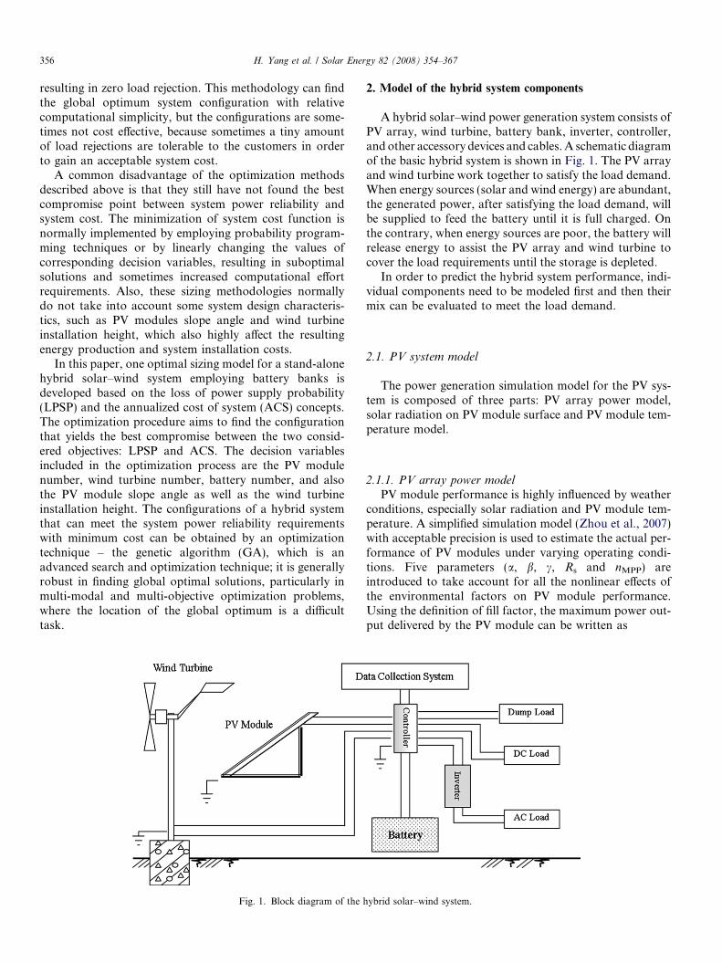
Fig. 1. Block diagram of the h

2. Model of the hybrid system components

A hybrid solar–wind power generation system consists ofPV array, wind turbine, battery bank, inverter, controller,and other accessory devices and cables. A schematic diagramof the basic hybrid system is shown in Fig. 1. The PV arrayand wind turbine work together to satisfy the load demand.When energy sources (solar and wind energy) are abundant,the generated power, after satisfying the load demand, willbe supplied to feed the battery until it is full charged. Onthe contrary, when energy sources are poor, the battery willrelease energy to assist the PV array and wind turbine tocover the load requirements until the storage is depleted.

In order to predict the hybrid system performance, indi-vidual components need to be modeled first and then theirmix can be evaluated to meet the load demand.

2.1. PV system model

The power generation simulation model for the PV sys-tem is composed of three parts: PV array power model,solar radiation on PV module surface and PV module tem-perature model.

2.1.1. PV array power model

PV module performance is highly influenced by weatherconditions, especially solar radiation and PV module tem-perature. A simplified simulation model (Zhou et al., 2007)with acceptable precision is used to estimate the actual per-formance of PV modules under varying operating condi-tions. Five parameters (a, b, c, Rs and nMPP) areintroduced to take account for all the nonlinear effects ofthe environmental factors on PV module performance.Using the definition of fill factor, the maximum power out-put delivered by the PV module can be written as

ybrid solar–wind system.

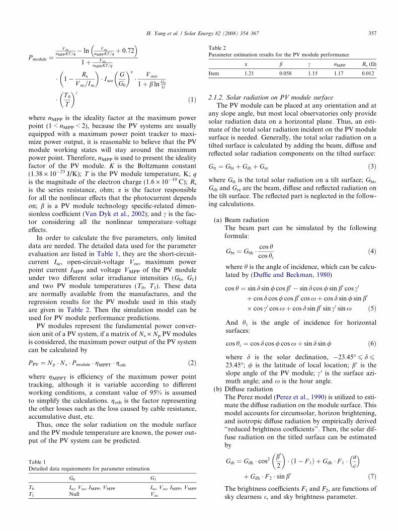
Table 2Parameter estimation results for the PV module performance

a b c nMPP Rs (X)

Item 1.21 0.058 1.15 1.17 0.012


P module ¼V oc

nMPPKT=q� ln V oc

nMPPKT=qþ 0:72� �

1þ V oc

nMPPKT=q

� 1� Rs

V oc=I sc

� �� I sco

GG0

� �a

� V oco

1þ b ln G0

G

� T 0

T

� �c

ð1Þ

where nMPP is the ideality factor at the maximum powerpoint (1 < nMPP < 2), because the PV systems are usuallyequipped with a maximum power point tracker to maxi-mize power output, it is reasonable to believe that the PVmodule working states will stay around the maximumpower point. Therefore, nMPP is used to present the idealityfactor of the PV module. K is the Boltzmann constant(1.38 · 10�23 J/K); T is the PV module temperature, K; q

is the magnitude of the electron charge (1.6 · 10�19 C); Rs

is the series resistance, ohm; a is the factor responsiblefor all the nonlinear effects that the photocurrent dependson; b is a PV module technology specific-related dimen-sionless coefficient (Van Dyk et al., 2002); and c is the fac-tor considering all the nonlinear temperature–voltageeffects.

In order to calculate the five parameters, only limiteddata are needed. The detailed data used for the parameterevaluation are listed in Table 1, they are the short-circuit-current Isc, open-circuit-voltage Voc, maximum powerpoint current IMPP and voltage VMPP of the PV moduleunder two different solar irradiance intensities (G0, G1)and two PV module temperatures (T0, T1). These dataare normally available from the manufactures, and theregression results for the PV module used in this studyare given in Table 2. Then the simulation model can beused for PV module performance predictions.

PV modules represent the fundamental power conver-sion unit of a PV system, if a matrix of Ns · Np PV modulesis considered, the maximum power output of the PV systemcan be calculated by

P PV ¼ N p � N s � P module � gMPPT � goth ð2Þ

where gMPPT is efficiency of the maximum power pointtracking, although it is variable according to differentworking conditions, a constant value of 95% is assumedto simplify the calculations. goth is the factor representingthe other losses such as the loss caused by cable resistance,accumulative dust, etc.

Thus, once the solar radiation on the module surfaceand the PV module temperature are known, the power out-put of the PV system can be predicted.

Table 1Detailed data requirements for parameter estimation

G0 G1

T0 Isc, Voc, IMPP, VMPP Isc, Voc, IMPP, VMPP

T1 Null Voc

2.1.2. Solar radiation on PV module surface

The PV module can be placed at any orientation and atany slope angle, but most local observatories only providesolar radiation data on a horizontal plane. Thus, an esti-mate of the total solar radiation incident on the PV modulesurface is needed. Generally, the total solar radiation on atilted surface is calculated by adding the beam, diffuse andreflected solar radiation components on the tilted surface:

Gtt ¼ Gbt þ Gdt þ Gre ð3Þ

where Gtt is the total solar radiation on a tilt surface; Gbt,Gdt and Gre are the beam, diffuse and reflected radiation onthe tilt surface. The reflected part is neglected in the follow-ing calculations.

(a) Beam radiationThe beam part can be simulated by the followingformula:

Gbt ¼ Gbh �cos hcos hz

ð4Þ

where h is the angle of incidence, which can be calcu-lated by (Duffie and Beckman, 1980)

cos h ¼ sin d sin / cos b0 � sin d cos / sin b0 cos c0

þ cos d cos / cos b0 cos xþ cos d sin / sin b0

� cos c0 cos xþ cos d sin b0 sin c0 sin x ð5Þ

And hz is the angle of incidence for horizontalsurfaces:

cos hz ¼ cos d cos / cos xþ sin d sin / ð6Þ

where d is the solar declination, �23.45� 6 d 623.45�; / is the latitude of local location; b 0 is theslope angle of the PV module; c 0 is the surface azi-muth angle; and x is the hour angle.

(b) Diffuse radiationThe Perez model (Perez et al., 1990) is utilized to esti-mate the diffuse radiation on the module surface. Thismodel accounts for circumsolar, horizon brightening,and isotropic diffuse radiation by empirically derived‘‘reduced brightness coefficients’’. Then, the solar dif-fuse radiation on the titled surface can be estimatedby

Gdt ¼ Gdh � cos2 b0

2

� �� ð1� F 1Þ þ Gdh � F 1 �

ac

� �

þ Gdh � F 2 � sin b0 ð7Þ

The brightness coefficients F1 and F2, are functions ofsky clearness e, and sky brightness parameter.

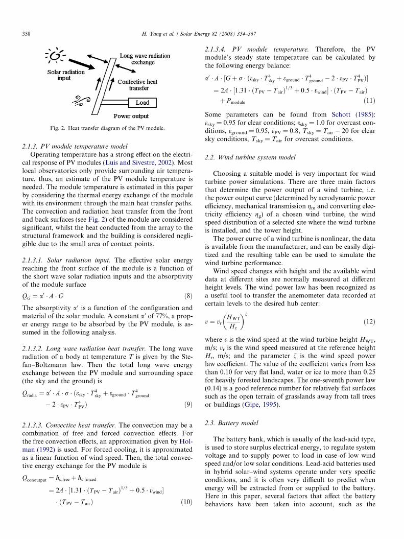
Fig. 2. Heat transfer diagram of the PV module.


2.1.3. PV module temperature model

Operating temperature has a strong effect on the electri-cal response of PV modules (Luis and Sivestre, 2002). Mostlocal observatories only provide surrounding air tempera-ture, thus, an estimate of the PV module temperature isneeded. The module temperature is estimated in this paperby considering the thermal energy exchange of the modulewith its environment through the main heat transfer paths.The convection and radiation heat transfer from the frontand back surfaces (see Fig. 2) of the module are consideredsignificant, whilst the heat conducted from the array to thestructural framework and the building is considered negli-gible due to the small area of contact points.

2.1.3.1. Solar radiation input. The effective solar energyreaching the front surface of the module is a function ofthe short wave solar radiation inputs and the absorptivityof the module surface

QG ¼ a0 � A � G ð8ÞThe absorptivity a 0 is a function of the configuration andmaterial of the solar module. A constant a 0 of 77%, a prop-er energy range to be absorbed by the PV module, is as-sumed in the following analysis.

2.1.3.2. Long wave radiation heat transfer. The long waveradiation of a body at temperature T is given by the Ste-fan–Boltzmann law. Then the total long wave energyexchange between the PV module and surrounding space(the sky and the ground) is

Qradia ¼ a0 � A � r � ðesky � T 4sky þ eground � T 4

ground

� 2 � ePV � T 4PVÞ ð9Þ

2.1.3.3. Convective heat transfer. The convection may be acombination of free and forced convection effects. Forthe free convection effects, an approximation given by Hol-man (1992) is used. For forced cooling, it is approximatedas a linear function of wind speed. Then, the total convec-tive energy exchange for the PV module is

Qconoutput ¼ hc;free þ hc;forced

¼ 2A � ½1:31 � ðT PV � T airÞ1=3 þ 0:5 � vwind�� ðT PV � T airÞ ð10Þ

2.1.3.4. PV module temperature. Therefore, the PVmodule’s steady state temperature can be calculated bythe following energy balance:

a0 � A � ½Gþ r � ðesky � T 4sky þ eground � T 4

ground � 2 � ePV � T 4PVÞ�

¼ 2A � ½1:31 � ðT PV � T airÞ1=3 þ 0:5 � vwind� � ðT PV � T airÞþ P module ð11Þ

Some parameters can be found from Schott (1985):esky = 0.95 for clear conditions; esky = 1.0 for overcast con-ditions, eground = 0.95, ePV = 0.8, Tsky = Tair � 20 for clearsky conditions, Tsky = Tair for overcast conditions.

2.2. Wind turbine system model

Choosing a suitable model is very important for windturbine power simulations. There are three main factorsthat determine the power output of a wind turbine, i.e.the power output curve (determined by aerodynamic powerefficiency, mechanical transmission gm and converting elec-tricity efficiency gg) of a chosen wind turbine, the windspeed distribution of a selected site where the wind turbineis installed, and the tower height.

The power curve of a wind turbine is nonlinear, the datais available from the manufacturer, and can be easily digi-tized and the resulting table can be used to simulate thewind turbine performance.

Wind speed changes with height and the available winddata at different sites are normally measured at differentheight levels. The wind power law has been recognized asa useful tool to transfer the anemometer data recorded atcertain levels to the desired hub center:

v ¼ vrH WT

H r

� �n

ð12Þ

where v is the wind speed at the wind turbine height HWT,m/s; vr is the wind speed measured at the reference heightHr, m/s; and the parameter f is the wind speed powerlaw coefficient. The value of the coefficient varies from lessthan 0.10 for very flat land, water or ice to more than 0.25for heavily forested landscapes. The one-seventh power law(0.14) is a good reference number for relatively flat surfacessuch as the open terrain of grasslands away from tall treesor buildings (Gipe, 1995).

2.3. Battery model

The battery bank, which is usually of the lead-acid type,is used to store surplus electrical energy, to regulate systemvoltage and to supply power to load in case of low windspeed and/or low solar conditions. Lead-acid batteries usedin hybrid solar–wind systems operate under very specificconditions, and it is often very difficult to predict whenenergy will be extracted from or supplied to the battery.Here in this paper, several factors that affect the batterybehaviors have been taken into account, such as the


charging current rate, the charging efficiency, the self-dis-charge rate as well as the battery capacity.

Most battery models mainly focus on three differentcharacteristics, i.e. the battery state of charge (SOC) as wellas the floating charge voltage (or the terminal voltage) andthe battery lifetime.

2.3.1. Battery state-of-charge (SOC)

Energy will be stored in the batteries when the powergenerated by the wind turbine and PV array is greater thanthe load. When power generation cannot satisfy the loadrequirements, energy will be extracted from the batteries,and the load will be cut off when power generation by bothwind turbine and PV array is insufficient and the storage isdepleted.

Like all chemical processes, the battery capacity is tem-perature dependent. Generally, the battery capacitychanges can be expressed by using the temperature coeffi-cient dC (Berndt, 1994):

C0bat ¼ C00bat � ð1þ dC � ðT bat � 298:15ÞÞ ð13Þ

where C0bat is the available or practical capacity of the bat-tery when the battery temperature is Tbat, Ah; C00bat is thenominal or rated capacity of the battery, which is the valueof the capacity given by the manufacturer as the standardvalue that characterizes this battery, Ah; a temperaturecoefficient of dC = 0.6% per degree, is usually used unlessotherwise specified by the manufacturer (Berndt, 1994).

For perfect knowledge of the real SOC of a battery, it isnecessary to know the initial SOC, the charge or dischargetime and the current. However, most storage systems arenot ideal, losses occur during charging and dischargingand also during storage periods. Taking these factors intoaccount, the SOC of the battery at time t + 1 can be simplycalculated by

SOCðt þ 1Þ ¼ SOCðtÞ � 1� r � Dt24

� �

þ IbatðtÞ � Dt � gbat

C0bat

ð14Þ

where r is the self-discharge rate which depends on theaccumulated charge and the battery state of health (Guaschand Silvestre, 2003), and a proposed value of 0.2% per dayis recommended. It is difficult to measure separate chargingand discharging efficiencies, so manufacturers usually spec-ify a round-trip efficiency. In this paper, the battery chargeefficiency is set equal to the round-trip efficiency, and thedischarge efficiency is 1.

The current rate of the battery at time t for the hybridsolar–wind system can be described by

IbatðtÞ ¼P PVðtÞ þ P WTðtÞ � P AC loadðtÞ=ginverter � P DC loadðtÞ

V batðtÞð15Þ

The inverter efficiency ginverter is considered to be 92%according to the load profile and the specifications of the

inverter. In this case, the wind turbine is assumed to haveDC output, so the use of a rectifier is not necessary. Butif the wind turbine is designed to connect to an AC grid,then the rectifier losses should be considered for the partof wind energy that has been rectified from AC to DC.

2.3.2. Battery floating charge voltage

The battery floating charge voltage response under bothcharging and discharging conditions is modeled by theequation-fit method, which treats the battery as a blackbox and expresses the battery floating charge voltage bya polynomial in terms of battery SOC and battery current

V 0bat ¼ A� ðSOCÞ3 þ B� ðSOCÞ2 þ C � SOCþ D ð16Þ

where V 0bat is the battery floating charge voltage, in order totake into account the temperature effect on battery voltagepredictions, the temperature coefficient dV is applied (Bern-dt, 1994)

V bat ¼ V 0bat þ dV � ðT bat � 298:15Þ ð17Þ

where Vbat is the calibrated voltage of the battery, after thetemperature effects have been considered. The temperaturecoefficient dV is assumed to be a constant of �4 mV/�C per2 V cell for the considered battery temperature range in thisresearch.

Parameters A, B, C and D in Eq. (16) are functions ofthe battery current I, and can be calculated by the follow-ing second degree polynomial equations:

A

B

C

D

0BBB@

1CCCA ¼

a1 a2 a3

b1 b2 b3

c1 c2 c3

d1 d2 d3

0BBB@

1CCCA

I2

I

1

0B@

1CA ð18Þ

The parameters a1,a2,a3, . . . ,d1,d2,d3 can be determinedusing the least squares fitting method by fitting the equa-tions to battery performance data (usually available fromthe manufacturer). The parameters for the battery usedin the following project analysis are calculated to be:

a1 a2 a3

b1 b2 b3

c1 c2 c3

d1 d2 d3

0BBB@

1CCCA

¼

�0:00152 0:05509 0:15782

0:00165 �0:05758 �0:39049

�0:00024 0:01018 0:52391

�0:00014 0:00795 1:86557

0BBB@

1CCCA I > 0

0:00130 0:00093 0:03533

�0:00201 �0:00803 �0:08716

0:00097 0:00892 0:22999

�0:00021 �0:00306 1:93286

0BBB@

1CCCA I < 0

8>>>>>>>>>>>>><>>>>>>>>>>>>>:

ð19Þ


where I > 0 represents the battery charging process, andI < 0 for the discharging process. Once these parametersare estimated, the battery model can be used for thesimulations.

2.3.3. Battery lifetime

Two independent limitations on the lifetime of batterybanks (the battery cycle life Ybat,c and the battery float lifeYbat,f) are employed.

Battery cycle life Ybat,c is the length of time that the bat-tery will last under normal cycles before it requires replace-ment; it depends on the depth of discharge of individualcycles. During the battery lifetime, a great number of indi-vidual cycles may occur, including the charging and dis-charging process, and every discharging process willresult in some depletion of the battery. Here the equivalentfull cycles (EFC) concept (Ashari and Nayar, 1999) hasbeen taken, an average EFC will be given, and after allthe equivalent cycles, the battery will need to be replaced.

The battery float life Ybat,f is the maximum length oftime that the battery will last before it needs replacement,regardless of how much or how little it is used. This limita-tion is typically associated with the damage caused by cor-rosion in the battery, which is strongly affected bytemperature. Higher ambient temperatures are more con-ducive to corrosion, so a battery installed in warm sur-roundings would have a shorter float life than oneinstalled in air-conditioned surroundings.

Considering these two lifetime aspects or limitations, thebattery will be exhausted either from use or from old age,depending on which one is shorter.

2.3.4. Battery simulation constraints

The battery SOC was used as a decision variable for thecontrol of battery overcharge and discharge protections.The case of overcharge may occur when higher power isgenerated by the PV array and wind turbine, or whenlow load demand exists. In such a case when the batterySOC reaches the maximum value, SOCmax = 1, the controlsystem intervenes and stops the charging process. On theother hand, if the state of charge decreases to a minimumlevel, SOCmin = 1 � DOD, the control system disconnectsthe load. This is important to prevent against batteriesshortening their lifetime or even their destruction. Also,for longevity of battery life, the maximum charging rate,SOC/5, is given as the upper limit.

3. Power reliability model based on LPSP concept

Because of the intermittent solar radiation and windspeed characteristics, which highly influence the resultingenergy production, power reliability analysis has been con-sidered as an important step in any system design process.A reliable electrical power system means a system has suf-ficient power to feed the load demand during a certain per-iod or, in other words, has a small loss of power supplyprobability (LPSP). LPSP is defined as the probability that

an insufficient power supply results when the hybrid system(PV array, wind turbine and battery storage) is unable tosatisfy the load demand (Yang et al., 2003). It is a feasiblemeasure of the system performance for an assumed orknown load distribution. A LPSP of 0 means the load willalways be satisfied; and an LPSP of 1 means that the loadwill never be satisfied. Loss of power supply probability(LPSP) is a statistical parameter; its calculation is not onlyfocused on the abundant or bad resource period. There-fore, in a bad resource year, the system will suffer from ahigher probability of losing power.

There are two approaches for the application of LPSP indesigning a stand-alone hybrid system. The first one isbased on chronological simulation. This approach is com-putationally burdensome and requires the availability ofdata spanning a certain period of time. The secondapproach uses probabilistic techniques to incorporate thefluctuating nature of the resource and the load, thus elim-inating the need for time-series data. Considering theenergy accumulation effect of the battery, to present thesystem working conditions more precisely, the chronologi-cal method is employed in this research. The objective func-tion, LPSP, from time 0 to T can then be described by

LPSP ¼PT

t¼0Power � failure � time

T

¼PT

t¼0TimeðP availableðtÞ < P neededðtÞÞT

ð20Þ

where T is the number of hours in this study with hourlyweather data input. The power failure time is defined asthe time that the load is not satisfied when the power gen-erated by both the wind turbine and the PV array is insuf-ficient and the storage is depleted (battery SOC falls belowthe allowed value SOCmin = 1 � DOD and still has notrecovered to the reconnection point). The power neededby the load side can be expressed as

P neededðtÞ ¼P AC loadðtÞginverterðtÞ

þ P DC loadðtÞ ð21Þ

and the power available from the hybrid system isexpressed by

P availableðtÞ ¼ P PV þ P WT þ C � V bat

�Min Ibat;max ¼0:2C0bat

Dt;C0bat � ðSOCðtÞ � SOCminÞ

Dt

� �

ð22Þ

where C is a constant, 0 for battery charging process and 1for battery discharging process. SOC(t) is the battery state-of-charge at time t, and it is calculated based on the batterySOC at the previous time t � 1 by using Eq. (14). The windturbine, as mentioned before, is assumed to have DC out-put, so the rectifier is not used. But if the wind turbine isdesigned to have AC output, then the rectifier losses shouldbe considered for the part of wind energy that has been rec-tified from AC to DC.


Using the above developed objective function accordingto the LPSP technique, for a given LPSP value for oneyear, a set of system configurations, which satisfy the sys-tem power reliability requirements, can be obtained.

4. Economic model based on ACS concept

The optimum combination of a hybrid solar–wind sys-tem can make the best compromise between the two con-sidered objectives: the system power reliability andsystem cost. The economical approach, according to theconcept of annualized cost of system (ACS), is developedto be the best benchmark of system cost analysis in thisstudy. According to the studied hybrid solar–wind system,the annualized cost of system is composed of the annual-ized capital cost Cacap, the annualized replacement costCarep and the annualized maintenance cost Camain. Fivemain parts are considered: PV array, wind turbine, battery,wind turbine tower and the other devices. The other devicesare the equipments that are not included in the decisionvariables, including controller, inverter and rectifier (if itis necessary when the wind turbine is designed to haveAC output). Then, the ACS can be expressed by

ACS ¼ CacapðPVþWindþ Batþ TowerþOthersÞþ CarepðBatÞ þ CamainðPVþWindþ Bat

þ TowerþOthersÞ ð23Þ

4.1. The annualized capital cost

The annualized capital cost of each component (PVarray, wind turbine, battery, wind turbine tower and theother devices) has taken into account the installation cost(including PV array racks and cables et al.), and they arecalculated by

Cacap ¼ Ccap � CRFði; Y projÞ ð24Þ

where Ccap is the initial capital cost of each component,US$; Yproj is the component lifetime, year; CRF is the cap-ital recovery factor, a ratio to calculate the present value ofan annuity (a series of equal annual cash flows). The equa-tion for the capital recovery factor is

CRFði; Y projÞ ¼i � ð1þ iÞY proj

ð1þ iÞY proj � 1ð25Þ

Table 3The costs and lifetime aspect for the system components

Initial capital cost Replacement cost Min

PV array 6500 US$/kW Null 65Wind turbine 3500 US$/kW Null 95Battery 1500 US$/kAh 1500 US$/kAh 50Tower 250 US$/m Null 6.5Other components 8000 US$ Null 80

The annual real interest rate i is related to the nominalinterest rate i 0 (the rate at which you could get a loan)and the annual inflation rate f by the equation given below.

i ¼ i0 � f1þ f

ð26Þ

4.2. The annualized replacement cost

The annualized replacement cost of a system componentis the annualized value of all the replacement costs occur-ring throughout the lifetime of the project. In the studiedhybrid system, only the battery needs to be replaced peri-odically during the project lifetime.

Carep ¼ Crep � SFFði; Y repÞ ð27Þ

where Crep is the replacement cost of the component (bat-tery), US$; Yrep is the component (battery) lifetime, year;SFF is the sinking fund factor, a ratio to calculate the fu-ture value of a series of equal annual cash flows. The equa-tion for the sinking fund factor is

SFFði; Y repÞ ¼i

ð1þ iÞY rep � 1ð28Þ

4.3. The maintenance cost

The system maintenance cost, which has taken the infla-tion rate f into account, is given as

CamainðnÞ ¼ Camainð1Þ � ð1þ f Þn ð29Þ

where Camain(n) is the maintenance cost of the nth year.The initial capital cost, replacement cost, maintenance

cost in the first year and the lifetime of each component(PV array, wind turbine, battery, tower and other devices)in this study are assumed as shown in Table 3.

The configuration with the lowest annualized cost ofsystem (ACS) is taken as the optimal one from the config-urations that can guarantee the required reliability ofpower supply.

5. System optimization model with genetic algorithm

Due to more variables and parameters that have to beconsidered, the sizing of the hybrid solar–wind systems ismuch more complicated than the single source power

aintenance costthe first year

Lifetime(year)

Interest rate i 0

(%)Inflation rate f

(%)

US$/kW 25 3.75 1.5US$/kW 25US$/kAh NullUS$/m 25

US$ 25


generating systems. This type of optimization includes eco-nomical objectives, and it requires the assessment of long-term system performance in order to reach the bestcompromise for both power reliability and cost. The mini-mization of the cost (objective) function is implementedemploying a genetic algorithm (GA), which dynamicallysearches for the optimal system configurations.

5.1. Genetic algorithm

A genetic algorithm (GA) is an advanced search andoptimization technique. It has been developed to imitatethe evolutionary principle of natural genetics. Comparedwith traditional methods (the direct exhaustive searchmethod and the gradient-directed search method) for func-tion optimization, one of the main advantages of the GA isthat it is generally robust in finding global optimal solu-tions, particularly in multimodal and multi-objective opti-mization problems.

Generally, a GA uses three operators (selection, crossoverand mutation) to imitate the natural evolution processes.

The first step of a genetic evaluation is to determine ifthe chosen system configuration (called a chromosome)passes the functional evaluation, provides service to theload within the bounds set forth by the loss of power sup-ply probability. If the evaluation qualified chromosome hasa lower annualized cost of system (ACS) than the lowestACS value obtained at the previous iterations, this systemconfiguration (chromosome) is considered to be the opti-mal solution for the minimization problem in this iteration.This optimal solution will be replaced by better solutions, ifany, produced in subsequent GA generations during theprogram evolution.

After the selection process, the optimal solution willthen be subject to the crossover and mutation operationsin order to produce the next generation population untila pre-specified number of generations have been reachedor when a criterion that determines the convergence issatisfied.

5.2. Methodology of the optimization model

The following optimization model is a simulation tool toobtain the optimum size or optimal configuration of ahybrid solar–wind system employing a battery bank interms of the LPSP technique and the ACS concept by usinga genetic algorithm. The flow chart of the optimizationprocess is illustrated in Fig. 3.

The decision variables included in the optimization pro-cess are the PV module number NPV, wind turbine numberNWT, battery number Nbat, PV module slope angle b 0 andwind turbine installation height HWT. A year of hourlydata including the solar radiation on the horizontal sur-face, ambient air temperature, wind speed and load powerconsumption are used in the model.

The initial assumption of system configuration will besubject to the following inequalities constraints:

MinðNPV;N wind;NbatÞP 0 ð30ÞH low 6 HWT 6 Hhigh ð31Þ0� 6 b0 6 90� ð32Þ

An initial population of 10 chromosomes, comprising the1st generation, is generated randomly and the constraintsdescribed by inequalities (30)–(32) are evaluated for eachchromosome. If any of the initial population chromosomesviolates the problem constraints then it is replaced by a newchromosome, which is generated randomly and fulfils theseconstraints.

The PV array power output is calculated according tothe PV system model by using the specifications of thePV module as well as the ambient air temperature and solarradiation conditions. The wind turbine performance calcu-lations need to take into account the effects of wind turbineinstallation height. The battery bank, with total nominalcapacity C0bat (Ah), is permitted to discharge up to a limitdefined by the maximum depth of discharge DOD, whichis specified by the system designer at the beginning of theoptimal sizing process.

The system configuration will then be optimized byemploying a genetic algorithm, which dynamically searchesfor the optimal configuration to minimize the annualizedcost of system (ACS). For each system configuration, thesystem’s LPSP will be examined for whether the loadrequirement (LPSP target) can be satisfied. Then, the lowercost load requirement satisfied configurations, will be sub-ject to the following crossover and mutation operations ofthe GA in order to produce the next generation populationuntil a pre-specified number of generations has beenreached or when a criterion that determines the conver-gence is satisfied.

So, for the desired LPSP value, the optimal configura-tion can be identified both technically and economicallyfrom the set of configurations by achieving the lowestannualized cost of system (ACS) while satisfying the LPSPrequirement.

6. Results and discussion

The proposed method has been applied to analyze onehybrid project, which is designed to supply power for atelecommunication relay station on a remote island, Dal-ajia Island in Guangdong Province, China. A 1300 WGSM base station RBS2206 (24 V AC), and a 200 Wmicrowave (24 V DC) are needed for the normal operationof the telecommunication station. According to the projectrequirements and technical considerations, a continuouspower consumption of 1500 W (1300 W AC and 200 WDC) is chosen to be the hybrid system load requirement.

The technical characteristics of the PV module and bat-tery as well as the wind turbines power curve used in thestudied project are given in Tables 4 and 5 and Fig. 4.The lead-acid batteries employed in the project arespecially designed for deep cyclic operation in consumer

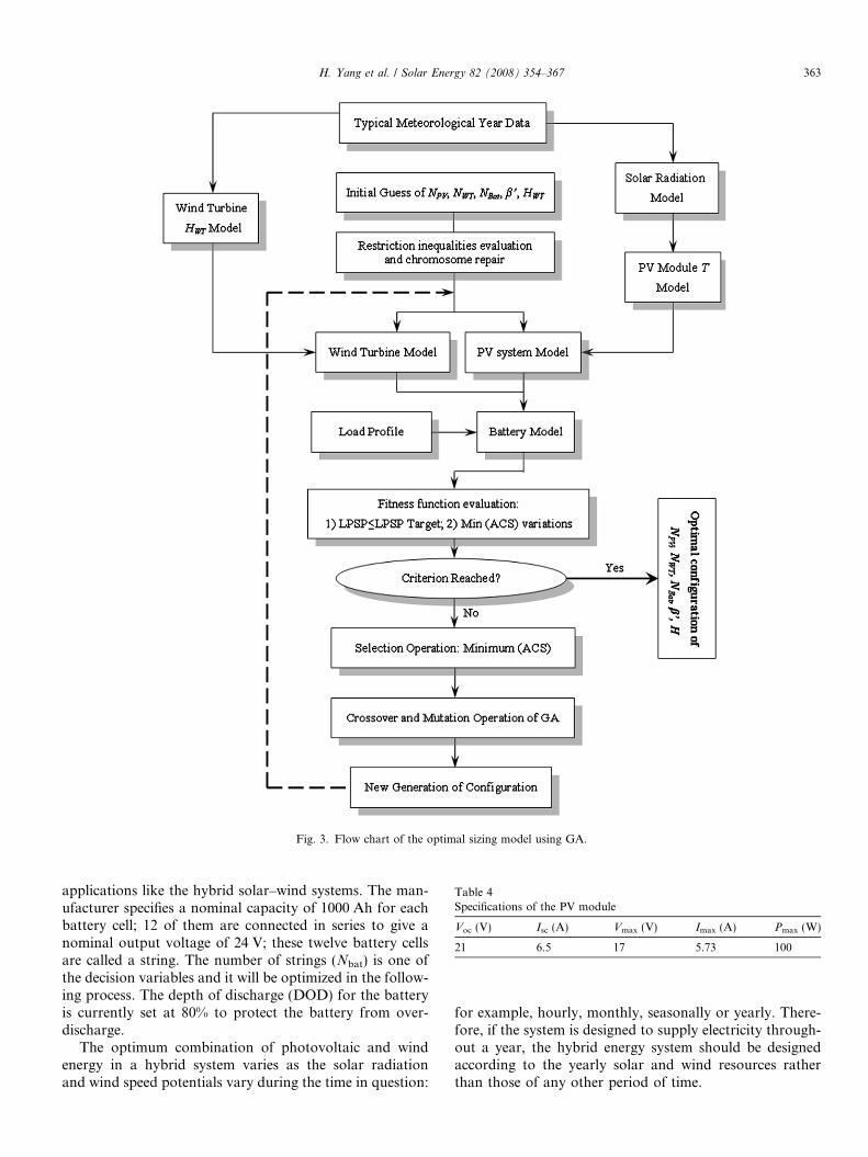
Fig. 3. Flow chart of the optimal sizing model using GA.

Table 4Specifications of the PV module

Voc (V) Isc (A) Vmax (V) Imax (A) Pmax (W)

21 6.5 17 5.73 100


applications like the hybrid solar–wind systems. The man-ufacturer specifies a nominal capacity of 1000 Ah for eachbattery cell; 12 of them are connected in series to give anominal output voltage of 24 V; these twelve battery cellsare called a string. The number of strings (Nbat) is one ofthe decision variables and it will be optimized in the follow-ing process. The depth of discharge (DOD) for the batteryis currently set at 80% to protect the battery from over-discharge.

The optimum combination of photovoltaic and windenergy in a hybrid system varies as the solar radiationand wind speed potentials vary during the time in question:

for example, hourly, monthly, seasonally or yearly. There-fore, if the system is designed to supply electricity through-out a year, the hybrid energy system should be designedaccording to the yearly solar and wind resources ratherthan those of any other period of time.

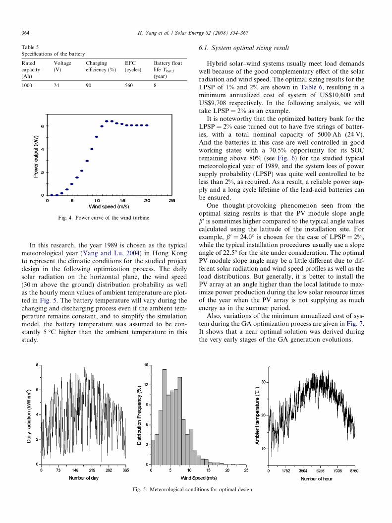
Table 5Specifications of the battery

Ratedcapacity(Ah)

Voltage(V)

Chargingefficiency (%)

EFC(cycles)

Battery floatlife Ybat,f

(year)

1000 24 90 560 8

Fig. 4. Power curve of the wind turbine.


In this research, the year 1989 is chosen as the typicalmeteorological year (Yang and Lu, 2004) in Hong Kongto represent the climatic conditions for the studied projectdesign in the following optimization process. The dailysolar radiation on the horizontal plane, the wind speed(30 m above the ground) distribution probability as wellas the hourly mean values of ambient temperature are plot-ted in Fig. 5. The battery temperature will vary during thechanging and discharging process even if the ambient tem-perature remains constant, and to simplify the simulationmodel, the battery temperature was assumed to be con-stantly 5 �C higher than the ambient temperature in thisstudy.

Fig. 5. Meteorological condi

6.1. System optimal sizing result

Hybrid solar–wind systems usually meet load demandswell because of the good complementary effect of the solarradiation and wind speed. The optimal sizing results for theLPSP of 1% and 2% are shown in Table 6, resulting in aminimum annualized cost of system of US$10,600 andUS$9,708 respectively. In the following analysis, we willtake LPSP = 2% as an example.

It is noteworthy that the optimized battery bank for theLPSP = 2% case turned out to have five strings of batter-ies, with a total nominal capacity of 5000 Ah (24 V).And the batteries in this case are well controlled in goodworking states with a 70.5% opportunity for its SOCremaining above 80% (see Fig. 6) for the studied typicalmeteorological year of 1989, and the system loss of powersupply probability (LPSP) was quite well controlled to beless than 2%, as required. As a result, a reliable power sup-ply and a long cycle lifetime of the lead-acid batteries canbe ensured.

One thought-provoking phenomenon seen from theoptimal sizing results is that the PV module slope angleb 0 is sometimes higher compared to the typical angle valuescalculated using the latitude of the installation site. Forexample, b 0 = 24.0� is chosen for the case of LPSP = 2%,while the typical installation procedures usually use a slopeangle of 22.5� for the site under consideration. The optimalPV module slope angle may be a little different due to dif-ferent solar radiation and wind speed profiles as well as theload distributions. But generally, it is better to install thePV array at an angle higher than the local latitude to max-imize power production during the low solar resource timesof the year when the PV array is not supplying as muchenergy as in the summer period.

Also, variations of the minimum annualized cost of sys-tem during the GA optimization process are given in Fig. 7.It shows that a near optimal solution was derived duringthe very early stages of the GA generation evolutions.

tions for optimal design.

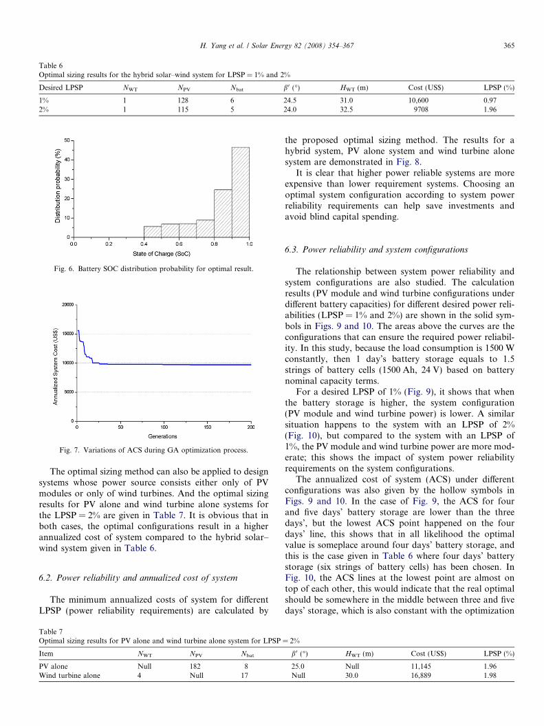
Table 6Optimal sizing results for the hybrid solar–wind system for LPSP = 1% and 2%

Desired LPSP NWT NPV Nbat b 0 (�) HWT (m) Cost (US$) LPSP (%)

1% 1 128 6 24.5 31.0 10,600 0.972% 1 115 5 24.0 32.5 9708 1.96

Fig. 6. Battery SOC distribution probability for optimal result.

Fig. 7. Variations of ACS during GA optimization process.


The optimal sizing method can also be applied to designsystems whose power source consists either only of PVmodules or only of wind turbines. And the optimal sizingresults for PV alone and wind turbine alone systems forthe LPSP = 2% are given in Table 7. It is obvious that inboth cases, the optimal configurations result in a higherannualized cost of system compared to the hybrid solar–wind system given in Table 6.

6.2. Power reliability and annualized cost of system

The minimum annualized costs of system for differentLPSP (power reliability requirements) are calculated by

Table 7Optimal sizing results for PV alone and wind turbine alone system for LPSP =

Item NWT NPV Nbat

PV alone Null 182 8Wind turbine alone 4 Null 17

the proposed optimal sizing method. The results for ahybrid system, PV alone system and wind turbine alonesystem are demonstrated in Fig. 8.

It is clear that higher power reliable systems are moreexpensive than lower requirement systems. Choosing anoptimal system configuration according to system powerreliability requirements can help save investments andavoid blind capital spending.

6.3. Power reliability and system configurations

The relationship between system power reliability andsystem configurations are also studied. The calculationresults (PV module and wind turbine configurations underdifferent battery capacities) for different desired power reli-abilities (LPSP = 1% and 2%) are shown in the solid sym-bols in Figs. 9 and 10. The areas above the curves are theconfigurations that can ensure the required power reliabil-ity. In this study, because the load consumption is 1500 Wconstantly, then 1 day’s battery storage equals to 1.5strings of battery cells (1500 Ah, 24 V) based on batterynominal capacity terms.

For a desired LPSP of 1% (Fig. 9), it shows that whenthe battery storage is higher, the system configuration(PV module and wind turbine power) is lower. A similarsituation happens to the system with an LPSP of 2%(Fig. 10), but compared to the system with an LPSP of1%, the PV module and wind turbine power are more mod-erate; this shows the impact of system power reliabilityrequirements on the system configurations.

The annualized cost of system (ACS) under differentconfigurations was also given by the hollow symbols inFigs. 9 and 10. In the case of Fig. 9, the ACS for fourand five days’ battery storage are lower than the threedays’, but the lowest ACS point happened on the fourdays’ line, this shows that in all likelihood the optimalvalue is someplace around four days’ battery storage, andthis is the case given in Table 6 where four days’ batterystorage (six strings of battery cells) has been chosen. InFig. 10, the ACS lines at the lowest point are almost ontop of each other, this would indicate that the real optimalshould be somewhere in the middle between three and fivedays’ storage, which is also constant with the optimization

2%

b 0 (�) HWT (m) Cost (US$) LPSP (%)

25.0 Null 11,145 1.96Null 30.0 16,889 1.98

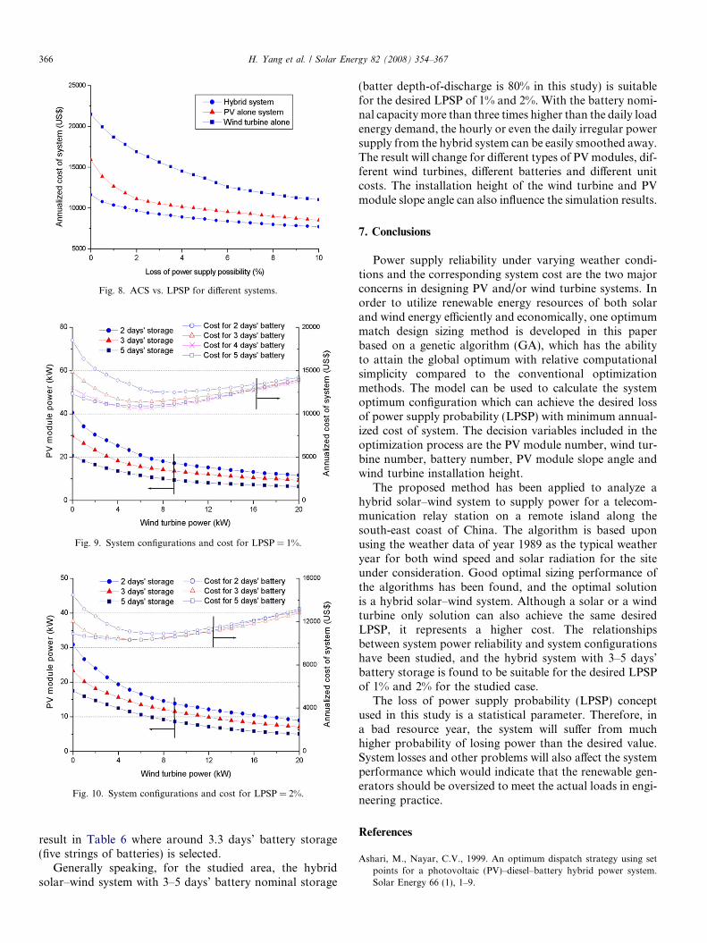
Fig. 8. ACS vs. LPSP for different systems.

Fig. 9. System configurations and cost for LPSP = 1%.

Fig. 10. System configurations and cost for LPSP = 2%.


result in Table 6 where around 3.3 days’ battery storage(five strings of batteries) is selected.

Generally speaking, for the studied area, the hybridsolar–wind system with 3–5 days’ battery nominal storage

(batter depth-of-discharge is 80% in this study) is suitablefor the desired LPSP of 1% and 2%. With the battery nomi-nal capacity more than three times higher than the daily loadenergy demand, the hourly or even the daily irregular powersupply from the hybrid system can be easily smoothed away.The result will change for different types of PV modules, dif-ferent wind turbines, different batteries and different unitcosts. The installation height of the wind turbine and PVmodule slope angle can also influence the simulation results.

7. Conclusions

Power supply reliability under varying weather condi-tions and the corresponding system cost are the two majorconcerns in designing PV and/or wind turbine systems. Inorder to utilize renewable energy resources of both solarand wind energy efficiently and economically, one optimummatch design sizing method is developed in this paperbased on a genetic algorithm (GA), which has the abilityto attain the global optimum with relative computationalsimplicity compared to the conventional optimizationmethods. The model can be used to calculate the systemoptimum configuration which can achieve the desired lossof power supply probability (LPSP) with minimum annual-ized cost of system. The decision variables included in theoptimization process are the PV module number, wind tur-bine number, battery number, PV module slope angle andwind turbine installation height.

The proposed method has been applied to analyze ahybrid solar–wind system to supply power for a telecom-munication relay station on a remote island along thesouth-east coast of China. The algorithm is based uponusing the weather data of year 1989 as the typical weatheryear for both wind speed and solar radiation for the siteunder consideration. Good optimal sizing performance ofthe algorithms has been found, and the optimal solutionis a hybrid solar–wind system. Although a solar or a windturbine only solution can also achieve the same desiredLPSP, it represents a higher cost. The relationshipsbetween system power reliability and system configurationshave been studied, and the hybrid system with 3–5 days’battery storage is found to be suitable for the desired LPSPof 1% and 2% for the studied case.

The loss of power supply probability (LPSP) conceptused in this study is a statistical parameter. Therefore, ina bad resource year, the system will suffer from muchhigher probability of losing power than the desired value.System losses and other problems will also affect the systemperformance which would indicate that the renewable gen-erators should be oversized to meet the actual loads in engi-neering practice.

References

Ashari, M., Nayar, C.V., 1999. An optimum dispatch strategy using setpoints for a photovoltaic (PV)–diesel–battery hybrid power system.Solar Energy 66 (1), 1–9.


Berndt, D., 1994. Maintenance-free Batteries. John Wiley & Sons,England.

Borowy, B.S., Salameh, Z.M., 1996. Methodology for optimally sizing thecombination of a battery bank and PV array in a wind/PV hybridsystem. IEEE Transactions on Energy Conversion 11 (2), 367–373.

Duffie, J.A., Beckman, W.A., 1980. Solar Engineering of Thermal Process.John Wiley & Sons, USA.

Eftichios, Koutroulis et al., 2006. Methodology for optimal sizing ofstand-alone photovoltaic/wind-generator systems using genetic algo-rithms. Solar Energy 80, 1072–1188.

Gipe, Paul, 1995. Wind Energy Comes of Age. John Wiley & sons, p. 536.Guasch, D., Silvestre, S., 2003. Dynamic battery model for photovoltaic

applications. Progress in Photovoltaics: Research and Applications 11,193–206.

Holman, J.P., 1992. Heat Transfer. McGraw-Hill.Kellogg, W.D. et al., 1998. Generation unit sizing and cost analysis for

stand-alone wind, photovoltaic and hybrid wind/PV systems. IEEETransactions on Energy Conversion 13 (1), 70–75.

Luis, C., Sivestre, S., 2002. Modeling Photovoltaic Systems using PSpice.John Wiley & Sons Ltd, Chichester.

Markvart, T., 1996. Sizing of hybrid PV-wind energy systems. SolarEnergy 59 (4), 277–281.

Perez, R., Ineichen, P., Seals, R., 1990. Modeling of daylight availabilityand irradiance components from direct and global irradiance. SolarEnergy 44, 271–289.

Schott, T., 1985. Operational temperatures of PV modules. In: 6th PVSolar Energy Conference. pp. 392–396.

Tina, G., Gagliano, S., Raiti, S., 2006. Hybrid solar/wind power systemprobabilistic modeling for long-term performance assessment. SolarEnergy 80, 578–588.

Van Dyk, E.E. et al., 2002. Long-term monitoring of photovoltaicdevices. Renewable Energy 22, 183–197.

Yang, H.X., Burnett, L., Lu, J., 2003. Weather data and probabilityanalysis of hybrid photovoltaic–wind power generation systems inHong Kong. Renewable Energy 28, 1813–1824.

Yang, H.X., Lu, L., 2004. Study on typical meteorological years and theireffect on building energy and renewable energy simulations. ASHRAETransactions 110 (2), 424–431.

Yang, H.X., Lu, L., Zhou, W., 2007. A novel optimization sizing modelfor hybrid solar–wind power generation system. Solar Energy 81 (1),76–84.

Zhou, W., Yang, H.X., Fang, Z.H., 2007. A novel model forphotovoltaic array performance prediction. Applied Energy 84 (12),1187–1198.

Documents

Optimal sizing method for stand-alone hybrid … · LPSP technology by using genetic algorithm ... ogy for optimal sizing of stand-alone PV/WG systems. The ... these sizing methodologies