OPTIMAL SENSOR POSITIONING ON PRESSURIZED EQUIPMENT BASED ON

VALUE OF INFORMATION

Seyed Mojtaba Hoseyni1, Francesco Di Maio1, Enrico Zio1,2,3

1Energy Department, Politecnico di Milano, Via La Masa 34, 20156 Milano, Italy

2MINES ParisTech / PSL Université Paris, Centre de Recherche sur les Risques et les Crises (CRC), Sophia

Antipolis, France

3Eminent Scholar, Department of Nuclear Engineering, Kyung Hee University

Abstract: In this work, we apply a simulation-based framework that makes use of the Value of Information (VoI)

for identifying the optimal spatial positioning of sensors on pressurized equipment. VoI is a utility-based Figure of

Merit (FoM) which quantifies the benefits/losses of acquiring information. Sensors are typically positioned on

pressurized equipment in line with specific recommendations based on operational experience, like UNI 11096 in

Italy. We show that the recommendations in UNI 11096 are, indeed, justified and that, incidentally, relying on VoI

for the optimization of the sensor positioning, one can achieve the same monitoring performance, as measured by VoI,

where following UNI 11096, but with a reduced number of sensors. The proposed VoI-based approach can, thus, be

used to confirm or revise recommendations coming from operational experience.

Keywords: Value of Information (VoI), Optimization, Sensors Positioning, Bayesian Statistics, Pressure

Vessel, Creep.

Acronyms

FoM Figure of Merit

GP Gaussian Process

NDT Non-Destructive Test

PFBR Prototype Fast Breeder Reactor

SG Steam Generator

SSC Systems, Structures, and Components

UTS Ultrasonic Thickness Testing

VoI Value of Information

Nomenclature

F Random field model

f(x) Random field at each spatial location x

f(x) Multivariate random field vector that affect the behavior of the system at each specific location x

x Location in the spatial domain

X Set of locations in the spatial domain Ωx

y(x) Measurement

Y Set of measurements in the spatial domain Ωy

y(x*) Optimal set of measurement

yn* Single sensor location that has the max VoI at the nth iteration of the greedy optimization algorithm

i Quantity of sensor locations in spatial domain Ωx

k Quantity of the realizations of measurement set y(x)

ε Noise vector

a Action vector

s State vector

𝛽 Reliability index

n Quantity of optimal sensors

ns Quantity of sensor locations that share the same uncertainty and geometry

R Matrix indicating which positions of the random field is observed

r VoI per sensor

CI Coefficient of improvement

Ωx Spatial domain of sensors locations

Ωy Spatial domain of measurements

𝑝 𝐹

Prior distribution of the random field f(x)

𝑝 𝐹|𝑦

Posterior distribution of the random field f(x)

PF Prior probability of failure

PF|y Posterior probability of failure

𝔼𝐿(∅) Prior expected loss

𝔼𝐿() Posterior expected loss

𝔼𝐹 Expected value over the prior field 𝑝 𝐹

𝔼𝐹|𝑦 Expected value over the posterior field 𝑝𝐹|𝑦

𝜇 𝐹 Prior mean of the random variable f(x)

𝜇 𝐹|𝑦

Posterior mean of the random variable f(x)

𝜇 Mean of the random variable f(x) derived from the measurement set

µg Mean of the limit state

σg Standard deviation of the limit state

ΣF Prior covariance matrix of the random variable f(x)

Σ𝐹| Posterior covariance matrix of the random variable f(x)

ΣY Covariance matrix of the measurement

Σε Covariance matrix of the noise

Cf Cost of failure

Cp Cost of failure prevention

VoIUNI VoI obtained by UNI 11096 sensor positioning

nUNI Number of sensors as for UNI 11096 sensor positioning

𝑟𝑈𝑁𝐼 VoI ratio for UNI 11096 sensor positioning

C Cost of measurement

𝑉𝑜𝐼 Value of information

M Benefit of conducting measurement

fs (x) Strength random field

ft (x) Failure threshold field

g(x) Limit state function

1. INTRODUCTION

Safety-critical Systems, Structures, and Components (SSCs) need to comply with safety standards.

Guidelines are developed for testing the compliance to the safety standards. However, the guidelines are

not necessarily resulting from a formal process and may involve shortcomings and over-conservatism which

may lead to unnecessary costs (1,2). Also, guidelines should not slow down industrial advancements but

rather flexibly reflect methodological developments and technological advancements (3). For example, let

us consider the Italian regulatory code UNI 11096 (4), the European norm EN 13445 (5), or the American

norm ASME Boiler & Pressure Vessel Code (BPVC) (6), all aimed at describing the positioning of

thickness sensors to monitor pressurized equipment that may suffer of creep, and all based on

experimental/operational past experience, such as in-service inspections and structural analyses (7). These

guidelines might be challenged when dealing with new SSCs on which there is limited experience.

In the context of SSCs creep, for example, market competition has pushed industry to operate the SSCs at

high design stresses (and, in some cases, beyond design stresses) (8,9), while new knowledge on creep

phenomenon becomes available. This has recently resulted in a deep revision of the guidelines (10,11),

making scheduled inspections by Non-Destructive Tests (NDTs) recommended to prevent SSCs creep and

failures (12,13,1,14). On the other hand, condition monitoring and intelligent analysis of data collected by

sensors may help predicting degradation escalation and anticipating the risk of failure (15,16,17,18,19).

In this work, we use the concept of Value of Information (VoI) to find how to optimally position ultrasonic

thickness gauges on a pressurized equipment, for largest benefit in terms of reduced costs and increased

data accuracy. VoI is a mathematical concept standing on Bayesian statistical decision theory and applied

in different fields for supporting decision making, from economics to engineering (20). For practical

meaning, we consider the problem of positioning sensors on a simulated manifold of a Steam Generator

(SG). The novelty of this work lies in use of the VoI-based sensors positioning framework for comparing

the outcomes with standards/recommendations/guidelines for monitoring of energy SSCs issued by

regulatory bodies, to confirm their validity or suggest improvements. Results show that the VoI based

sensor positioning allows reducing the number of sensors to be positioned with respect to the guidelines in

(4), while achieving the same VoI. This shows that guidelines can benefit from VoI and simulation to obtain

cost-effective solutions that overcome the shortcomings of relying only on past operational experience.

The paper is organized as follows. Section 2 introduces the VoI concept and presents the framework that

uses VoI and simulation for optimal positioning of sensors. Section 3 illustrates the case study that consists

in the positioning of sensors on a SG; the solution for sensors positioning obtained following the guideline

in UNI 11096 is benchmarked with that derived from the proposed VoI-based approach. Section 4

concludes the paper with some remarks.

2. Value of Information

Value of Information (VoI) is a mathematical concept used in Bayesian statistical decision theory to

quantify (in monetary terms) the gain that one could obtain by updating prior available information with

new one, before adopting it (21). Indeed, the process of acquiring information (here specifically consisting

in measurements from sensors) may not always be justified because of the high cost, and one finds this out

only after (the information is acquired by the measurements taken) (22,23). In other words, VoI predicts

(by simulation) the economic benefit of collecting measurements in specific sensors locations, by

accounting (in addition to the cost of the sensor and measurement acquisition chain) for the costs that the

decision-maker might incur when adopting mitigative actions to counteract SSC degradation (or its failure,

in case no action is taken) based on the collected measurements. This provides a powerful tool for

comparing different locations of measurement before physically placing the sensors on the SSCs (i.e., a

location that has larger VoI value is more beneficial) and makes it possible to find the most beneficial set

by solving an optimization problem that finds the observation that has the largest VoI.

The mathematical framework for quantifying the VoI is recalled in the following: In general terms, a spatial

domain Ωx can be defined over the SSC of interest and indicated by its spatial coordinates. For example,

each location on a 2-dimensional Ωx can be indicated as x = x1, x2. For practicality, the spatial domain Ωx

is discretized into a finite set of i locations X = x1, x2, …, xi. A spatial model F= f(x) can be introduced on

the spatial domain Ωx to measure a certain property of the SSC at each location x (e.g., for a pressurized

vessel, a random field f(x) of stress, at each location x). If multiple random fields f(x) (e.g., stress,

temperature, thickness and so on) insist on the SSC, F = f(x) can be defined as a multivariate random field,

possibly with dependencies (24).

The spatial model can be described based on design values and operational experience (i.e., prior

knowledge), eventually assigning prior distributions 𝑝 𝐹 of values to the relevant variables (e.g., the

distribution of the internal stress in a pressurized vessel).

Similar to the spatial domain Ωx, the measurements spatial domain Ωy can be defined at locations x = x1,

x2 where the measurements can be taken (i.e., Ωy ⊆ Ωx). The measurement set y(x) is the collection of

measurements at the generic location x (e.g., measurements of realizations of the multivariate random field

f(x)). Then, Y is defined as the set of measurements y(x) at the selected locations x:

𝑦 (𝑥 ) = R(𝑥 ) + (1)

where R is a row matrix indicating which locations in Ωx are observed (i.e., R is a row matrix with zero

value for the non-observed locations of X and 1 for the observed locations), and ε is a vector of random

noise measurements, usually assumed to be distributed like a Gaussian with zero mean and covariance

matrix Σε (24). When new information become available (new measurements are recorded), the distribution

of the model f(x) can be updated. Specifically, Bayesian inference allows updating the prior distributions

𝑝 𝐹 to obtain the posterior distribution 𝑝 𝐹|𝑦 .

Prior and posterior distributions, 𝑝 𝐹 and 𝑝 𝐹|𝑦 can be used by a decision-maker to decide an action from a

set of possible actions a. In particular, the SSCs prior probability of failure PF (x) and posterior probability

of failure PF|y (x) that can be inferred from 𝑝 𝐹 and 𝑝 𝐹|𝑦 , respectively, can support, in a risk-informed

perspective, a decision-maker choice of maintenance by balancing risk and actions costs, on the basis of

the most informative set that can be collected.

To this aim, a loss function L(f (x), a) can be introduced as negative utility (i.e., loss) that may come from

taking a decision. For example, in case a decision of action is taken based only on the prior knowledge 𝑝 𝐹

without relying on additional measurements (∅), the prior expected loss 𝔼L(∅) can be minimized to find

the optimal action:

𝔼𝐿(∅) = 𝑚𝑖𝑛𝔼𝐹𝐿((𝑥 ), 𝑎 ) (2)

On the other hand, if y(x) is available, the decision can be taken a posteriori of collecting the information

y(x), i.e., with respect to 𝑝 𝐹|𝑦 , and minimizing the posterior expected loss 𝔼𝐿(𝑦 (𝑥 )):

𝔼𝐿(𝑦 (𝑥 )) = 𝔼𝑌min𝔼𝐹|𝑦 𝐿((𝑥 ), 𝑎 ) (3)

For example, based on 𝑝 𝐹 (e.g. the prior knowledge on the field of stress on a plate with growing cracks,

providing a failure probability estimate PF(x) due to the load applied) a repair decision might be taken that

differs from the one that would have been taken if the posterior probability of failure PF|y(x) would have

been considered, if PF|y(x) were updated with the new measurements y(x) that have become available.

For the pressurized vessel, 𝑝 𝐹|𝑦 reflects the updated distribution of the stress, conditioned on the collected

information y(x): within the here proposed simulation-based approach, the measurement corresponds to a

random realizations in a specific location i. To account for this stochasticity, we assume that in each

location, we simulate the collection of K alternative measurements, and 𝑝 𝐹 and 𝑝 𝐹|𝑦 are collected

accordingly with their consequent losses as in Equations (2) and (3). K different stochastic realizations of

𝑦 (𝑥 𝑖) represent K different posterior expected losses (𝔼𝐿(𝑦 (𝑥 𝑖))𝑘 which are averaged to quantify the

posterior expected loss conditioned on the measurement at a specific location i as:

𝔼𝐿(𝑦 (𝑥 𝑖)) =∑ (𝔼𝐿(𝑦 (𝑥 𝑖))𝑘𝐾𝑘=1

𝐾 (4)

The difference between 𝔼L(∅) and 𝔼𝐿(𝑦 (𝑥 )) quantifies the benefit of taking decisions informed by the

new information 𝑦 (𝑥 ), and is, thus, the VoI:

VoI (𝑦 (𝑥 )) = 𝔼L(∅) − 𝔼L(𝑦 (𝑥 )) (5)

2.1. VoI-based sensor positioning

As mentioned before, decisions are made optimal by the informativeness of y(x). The cost-effectiveness of

y(x) holds when its cost C(y(x)) is less than (or equal) to the VoI gained (i.e., VoI(𝑦 (𝑥 ))≥ C(y(x))), and the

utility M(𝑦 (𝑥 ))≥ 0:

M(𝑦 (𝑥 )) = VoI (𝑦 (𝑥 )) − C(𝑦 (𝑥 )) (6)

The optimal set of measurement y(x*), i.e., the set which maximizes the utility M(y(x)), is determined by

the optimal number of sensors n and their positioning. In principle, the optimal positioning of sensors can

be found by simulating every possible set of measurement location on Ωy by a combinatorial and

computationally impractical way of solving Equation (7):

∗(𝑥 ) = 𝑎𝑟𝑔𝑚𝑎𝑥 𝑌 ⊆𝛺𝑌 (𝑀()) (7)

Alternatively, optimization approaches can be used: in greedy optimization approach, firstly the optimal

positioning for a single sensor is searched by simulation (i.e., n = 1) and, then, based on this result, the next

sensor is positioned until, iteratively, the maximum desired M() is reached by updating the nth 𝑝 𝐹 from the

(n-1)th 𝑝 𝐹|𝑦 to take into account the availability of new measurements taken at the selected location (25,26).

2.2. VoI-based sensor positioning for Gaussian fields

A particular case of the sensor positioning procedure described in Section 2.1 is the sensor positioning on

Gaussian fields, which means that f(x) is normally distributed on Ωx (27), with a mean function value m(x),

a standard deviation 𝜎(𝑥 ), and covariance k(x, x′) with correlation ρ(x, x′) (i.e., 𝑘(𝑥 , 𝑥 ′) = 𝜎(𝑥 )𝜎(𝑥 ′)𝜌(𝑥 , 𝑥 ′))

between locations x and x′. This means, also, that when a measurement is taken at a given location (𝑥1, 𝑥2),

any other measurement at any other location (𝑥1′, 𝑥2′) is correlated with (𝑥1, 𝑥2) according to the exponential

correlation function (28):

ρ(𝑥1, 𝑥2, 𝑥1′ , 𝑥2

′ ) = exp ( -√((𝑥1−𝑥1

′)2+(𝑥2−𝑥2

′)2)

𝜆2) (8)

where 𝜆 is called scale parameter (in the case study of Section 3, 𝜆 is taken equal to 100 mm).

In various cases, spatially distributed systems can be assumed to be Gaussian (29,28) and, Bayesian

inference for the sensors positioning can exploit the property of conjugate priors (30), as discussed

hereafter.

Specifically:

• the multivariate field f(x) can be described by the mean vector 𝜇 𝐹 = (𝑥 ) containing multivariate

mean values m(x) of different SSC properties and a covariance matrix ΣF = 𝑘(𝑥 , 𝑥 ′), with a prior

distribution 𝑝 𝐹:

𝑓(𝑥 ) ~ 𝑝 𝐹= ℕ(𝜇

𝐹, Σ𝐹) (9)

• the measurement set y(x) of Equation (1) is modeled as an independent, identically distributed, zero

mean Gaussian distribution covariance matrix Σε can be described as distributed by a multivariate

normal distribution with 𝜇 = R𝜇 𝐹 ,Σ = RΣFRT + Σε (Equation (10)):

𝑦 (𝑥 ) ~ 𝑝 𝐹|𝑦 = ℕ(𝜇 , Σ) (10)

The conjugate posterior of f(x) is, thus, a Gaussian distribution (31):

𝑓 | 𝑦 (𝑥 ) ~ ℕ (µ 𝐹|𝑦 , Σ𝐹|) (11)

with:

𝜇 𝐹|𝑦 = 𝜇 𝐹 + Σ𝐹RTΣ

−1(𝑦 (𝑥 )− 𝜇 ) (12)

and

Σ𝐹| = Σ𝐹 − Σ𝐹RTΣ

−1RΣ𝐹 (13)

being the posterior mean and covariance, respectively.

3. Application of the VoI-based Approach for Optimal Sensor

Positioning on a SG Undergoing Creep

The application of the VoI-based approach for sensor positioning described in Section 2.1. is here shown

with respect to the optimization of sensors positioning on a manifold of the SG of a Prototype Fast Breeder

Reactor (PFBR) (See Figure 1), whose thickness can be measured by Ultrasonic Thickness Testing (UTS).

Figure 1:The manifold of a SG of a PFBR used as test case for the VoI-based approach for sensor positioning

Under the assumed operating conditions listed in Table 1, the manifold may suffer of creep due to the large

design pressure and temperature, and long exposure time that may lead to failure.

Table 1: Operating conditions of the SG

Design pressure 189 barg

Design temperature 778 °K = 505 °C inlet

723 °K = 450 °C outlet

Material 9Cr-1Mo-V-Nb (Plate)

ASME SA-387/SA-387M Grade 91

Percentage of life

spent 35%

Operating hours 100,000 h

Tensile strength 475 MPa

Thickness 20 mm

Failure would occur at location x if the thickness (i.e., the Gaussian strength random field fs (x)) is smaller

than a threshold thickness, here assumed equal to a constant value of 16.9 mm on the whole Ωx (i.e., the

failure threshold field ft (x) calculated in (32) in line with (33) using the NIMS creep database (34), that

contains creep data collected in experiments related to pressurized equipment of NPP of the same material

and operating under the same conditions of the manifold considered in our case).

Since fs (x) is a Gaussian field and ft (x) is a constant, the limit state function 𝑔(𝑥 ) = 𝑓𝑠(𝑥 ) − 𝑓𝑡(𝑥 ) is a

Gaussian g(x) ~ N (µg(x), σg(x)), which implies a probability of manifold failure P(x) (i.e. the probability

that g(x)<0) equal to:

(𝑥 ) = Φ(−β(𝑥 )) (14)

where Φ(.) is the standard normal cumulative distribution function, and 𝛽 is the reliability index equal to:

𝛽(𝑥 ) = 𝜇𝑔(𝑥 )

𝜎𝑔(𝑥 ) (15)

The technical procedure in the Italian guideline ISPESL n. 48/2003 (33) and, specifically, the norm (UNI

11096, 2012) (4) is used as benchmark for the sensors positioning. In line with (4), 32 thickness gauges are

placed in the locations (*) of Figure 2, among 160 locations available. Notice that holes of subchannels

within the manifold are neglected in line with (4).

Figure 2: Schematic view of the unwrapped manifold with sensor locations (x), in line with (UNI 11096, 2012).

This benchmark positioning is, however, independent from the actual fs (x) that may vary, due to the

manifold production process. The following common cases are considered (see Figure 3):

1. Circumferential welding of two extruded manifolds.

2. Longitudinal welding of a rectangular plate.

3. Circumferential welding of two manifolds resulting from a longitudinal welding of two rectangular

plates.

4. Manifold extrusion.

Figure 3: schematic view of the four case studies.

In all these cases, the fs (x) is modeled with a Gaussian model 𝑝 𝐹(𝑥 ) = ℕ ~ (20mm, 1mm) except for the

welding and Heat Affected Zone (HAZ), where 𝑝 𝐹(𝑥 ) of fs (x) is ℕ ~ (20mm, 2mm). Figure 4 shows the

standard deviation of fs (x) for all the cases (the lighter the color, the larger the standard deviation).

Figure 4: Standard deviation of fs (x) for the four case studies

Knowing that ft (x) is equal to 16.9 mm, the prior probability of failure PF (x) can be calculated at any

location x of the manifold, as plotted in Figure 5 (the warmer the color, the larger the probability of failure).

Figure 5: Prior probability of failure PF (x) for the four case studies

At this point, it can be decided to: 1. do nothing (a = 0) with zero cost, or 2. mitigate degradation (a = 1)

(for, example, for mitigating creep, one can either reduce the operational stress (i.e., lowering pressure,

temperature, …), or sleeve the risky area, or perform a weld repair (35), or any combination of these with

cost Cm). Depending on the true state (s) of the manifold, unknown to the decision maker, (i.e., too much

degraded (s = 0) that would entail failure cost of Cf, or operational (s = 1)), one sets the loss function value:

𝐿(𝑓(𝑥 ), ) =

0 𝑖𝑓 𝑠 = 1 𝑎𝑛𝑑 𝑎 = 0𝐶𝑓 = 200𝐾€ 𝑖𝑓 𝑠 = 0 𝑎𝑛𝑑 𝑎 = 0

𝐶𝑚 = 5𝐾€ 𝑖𝑓 𝑎 = 1

(16)

In other words, if no mitigation action is performed (a = 0) and the true state is operational (s = 1), then

the decision comes with zero cost; otherwise, if the actual state is too degraded (s = 0), then, a wrong

decision comes with cost Cf . It is assumed that, regardless of the true state of the manifold, if a failure

mitigation action is undertaken, the payoff is the cost Cm.

For the proposed application, the prior expected loss 𝔼L(∅) = ∑ 𝔼𝐿𝑖(∅)160𝑖=1 is quantified by simultaneously

accounting for all the 160 prior expected losses, where, for the 𝑖-th location, the prior expected loss is:

𝔼𝐿𝑖(∅) = 𝑚𝑖𝑛𝔼𝐹𝐿𝑖(𝑓(𝑖), 𝑖) = 𝑚𝑖𝑛𝔼𝐹𝐿𝑖(𝑓(𝑖), 0), 𝔼𝐹𝐿𝑖(𝑓(𝑖), 1) = 𝑚𝑖𝑛𝐶𝑓 × 𝑃𝐹 (𝑖), 𝐶𝑚 (17)

being 𝔼𝐹𝐿𝑖(𝑓(𝑖), 0) the failure cost 𝐶𝑓 = 200 𝐾€ weighted by the probability of failure 𝑃𝐹(𝑖) (if no action

is taken, a=0), and 𝔼𝐹𝐿𝑖(𝑓(𝑖), 1) corresponds to the cost 𝐶𝑚 = 5𝐾€ (if maintenance action is taken, a=1).

Also the posterior expected loss 𝔼L(𝑦 (𝑥 )) = ∑ 𝔼𝐿𝑖(𝑦 (𝑥 ))160𝑖=1 is quantified by simultaneously accounting

for all the 160 posterior expected losses where, for the 𝑖-th location, the posterior expected loss conditional

on the measurement set 𝑦 (𝑥 ) is:

𝔼𝐿𝑖(𝑦 (𝑥 )) = 𝑚𝑖𝑛𝐶𝑓 × 𝑃𝐹|𝑦 (𝑖), 𝐶𝑚 (18)

being 𝑃𝐹|𝑦 (𝑖) the posterior probability of failure of location 𝑖.

It is worth mentioning that 𝔼L(∅) and 𝔼L(𝑦 (𝑥 )) have been calculated as the sum of all the prior and posterior

losses, respectively, of all the 160 locations, because we conservatively assume that the manifold integrity

is lost when at least one measurement location is overlooked ignoring the necessary mitigative action to

counteract manifold failure.

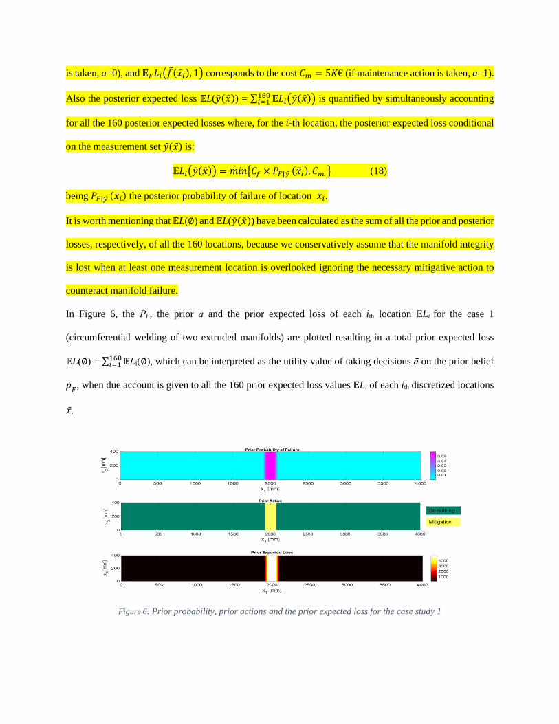
In Figure 6, the PF, the prior a and the prior expected loss of each ith location 𝔼Li for the case 1

(circumferential welding of two extruded manifolds) are plotted resulting in a total prior expected loss

𝔼L(∅) = ∑ 𝔼Li(∅)160𝑖=1 , which can be interpreted as the utility value of taking decisions a on the prior belief

𝑝 𝐹, when due account is given to all the 160 prior expected loss values 𝔼Li of each ith discretized locations

𝑥 .

Figure 6: Prior probability, prior actions and the prior expected loss for the case study 1

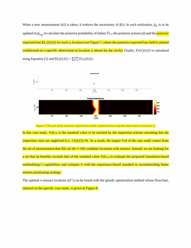
When a new measurement y(x) is taken, it reduces the uncertainty of f(x). In each realization, 𝑝 𝐹 is to be

updated in 𝑝 𝐹|𝑦 to calculate the posterior probability of failure PF|y, the posterior actions (a) and the posterior

expected loss 𝔼𝐿𝑖(𝑦 (𝑥 )) for each ith location (see Figure 7, where the posterior expected loss field is plotted

conditioned on a specific observation at location xo shown by the circle). Finally, 𝑉𝑜𝐼(𝑦 (𝑥 )) is calculated

using Equation (5) and 𝔼L(𝑦 (𝑥 )) = ∑ ELi(𝑦 (𝑥 ))160𝑖=1 .

Figure 7: The plot of the posterior expected loss field, conditioned on a specific observation at location xo.

In this case study, VoIUNI is the standard value to be reached by the inspection scheme assuming that the

inspection costs are neglected (i.e., C(𝑦 (𝑥 ))=0). As a result, the largest VoI of the case study comes from

the set of measurement that fills all the i=160 candidate locations with sensors. Instead, we are looking for

a set that its benefits exceeds that of the standard value VoIUNI to evaluate the proposed simulation-based

methodology’s capabilities and compare it with the experience-based standard in recommending better

sensors positioning strategy.

The optimal n sensors locations y(x*) can be found with the greedy optimization method whose flowchart,

tailored on the specific case study, is given in Figure 8.

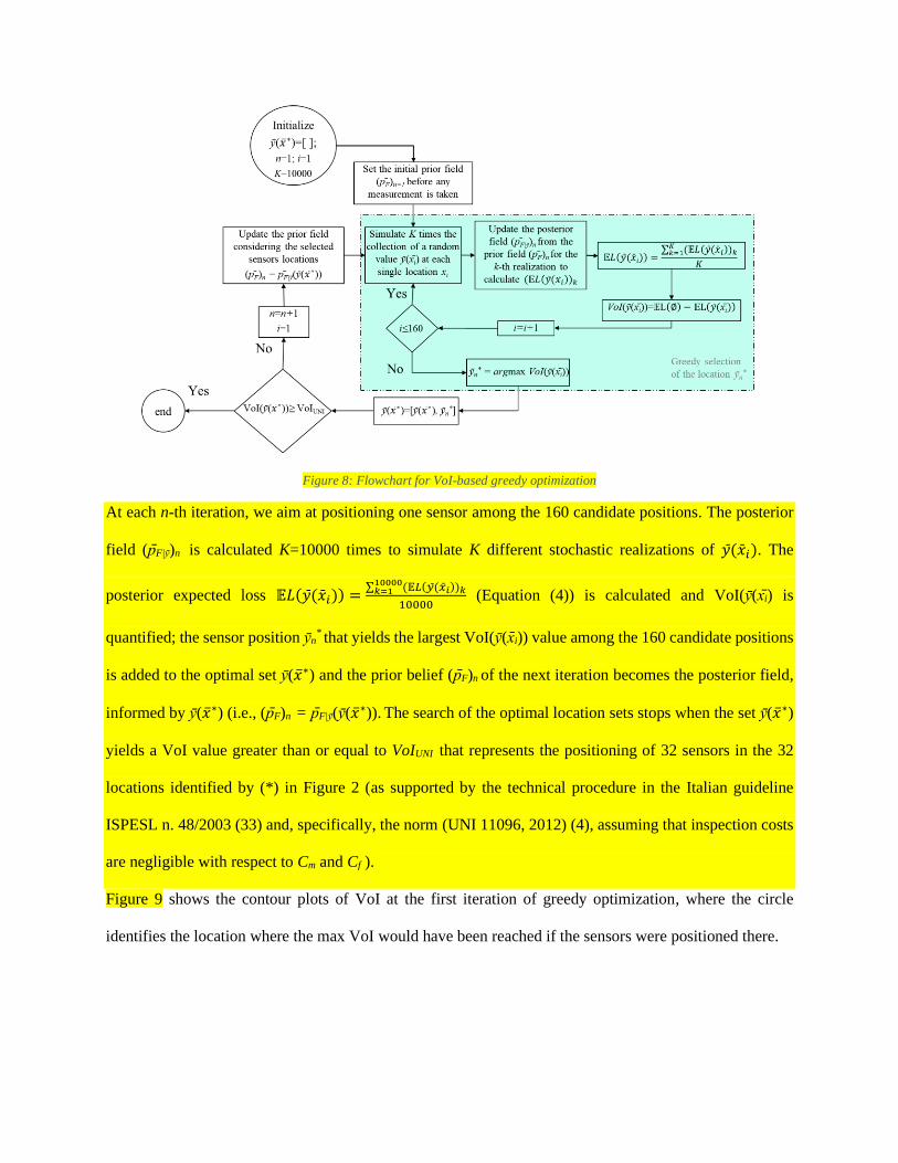
Figure 8: Flowchart for VoI-based greedy optimization

At each n-th iteration, we aim at positioning one sensor among the 160 candidate positions. The posterior

field (pF|y)n is calculated K=10000 times to simulate K different stochastic realizations of 𝑦 (𝑥 𝑖). The

posterior expected loss 𝔼𝐿(𝑦 (𝑥 𝑖)) =∑ (𝔼𝐿(𝑦 (𝑥 𝑖))𝑘10000𝑘=1

10000 (Equation (4)) is calculated and VoI(y(xi) is

quantified; the sensor position yn* that yields the largest VoI(y(xi)) value among the 160 candidate positions

is added to the optimal set y(∗) and the prior belief (pF)n of the next iteration becomes the posterior field,

informed by y(∗) (i.e., (pF)n = pF|y(y(∗)). The search of the optimal location sets stops when the set y(∗)

yields a VoI value greater than or equal to VoIUNI that represents the positioning of 32 sensors in the 32

locations identified by (*) in Figure 2 (as supported by the technical procedure in the Italian guideline

ISPESL n. 48/2003 (33) and, specifically, the norm (UNI 11096, 2012) (4), assuming that inspection costs

are negligible with respect to Cm and Cf ).

Figure 9 shows the contour plots of VoI at the first iteration of greedy optimization, where the circle

identifies the location where the max VoI would have been reached if the sensors were positioned there.

Figure 9: VoI contours for the four case studies at the first iteration n=1.

It can be seen that locations close to the HAZ (with larger uncertainty) also have larger VoI; a further proof

comes from the case study 4, for which all locations have the same 𝑝 𝐹 and, therefore, the VoI for any i-th

location is almost identical with (all other locations (i.e., slight difference in VoI is due to the stochasticity

of the random field characterization)).

Figure 10 shows the optimal sensors positions y(x*) for each of the case studies. The number of sensors n

required to exceed VoIUNI is 5, 17, 18, 32, respectively (where the numbers indicate the order of positions

selected by the optimization strategy).

Figure 10: Sensor positioning using the greedy optimization algorithm for the four case studies

In all cases, n< nUNI=32 and the ratio r = 𝑉𝑜𝐼

𝑛 is defined to show the VoI-per-sensor in each case study.

Similarly, 𝑟𝑈𝑁𝐼 = VoIUNI

𝑛UNI shows the VoI-per-sensor obtained by positioning by the (4) guidelines with

nUNI=32. Table 2 compares quantitatively the VoI, number of sensors n, and the VoI-per-sensor ratio r in

the different case studies, with their corresponding values of the (UNI 11096, 2012) sensors positioning.

The VoI-per-sensor ratio r of the case studies are compared with their associated rUNI values, with the

coefficient of improvement CI showing how much the VoI-per-sensor ratio r is improved using the

suggested framework (CI= 𝒓

𝒓𝑼𝑵𝑰).

Table 2: Comparison between the UNI 11096 and the proposed method for sensor positioning

Case

Study

VoI n r VoIUNI nUNI 𝒓𝑼𝑵𝑰 CI

1 2.6495e+04 5 5299 2.6386e+04 32 824.56 6.43

2 9.9772e+04 17 5868.94 9.4014e+04 32 2937.94 2.00

3 1.0727e+05 18 5959.44 1.0420e+05 32 3256.23 1.83

4 6.1561e+03 28 219.86 5.9847e+03 32 187.02 1.18

It can be seen that the VoI-based sensor positioning strategy in all cases gives a better VoI-per-sensor than

following the normative recommendation of (4).

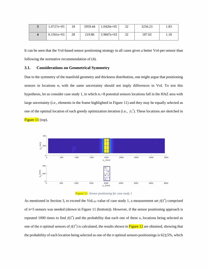
3.1. Considerations on Geometrical Symmetry

Due to the symmetry of the manifold geometry and thickness distribution, one might argue that positioning

sensors in locations ns with the same uncertainty should not imply differences in VoI. To test this

hypothesis, let us consider case study 1, in which ns=8 potential sensors locations fall in the HAZ area with

large uncertainty (i.e., elements in the frame highlighted in Figure 11) and they may be equally selected as

one of the optimal location of each greedy optimization iteration (i.e., yn*). These locations are sketched in

Figure 11 (top).

Figure 11: Sensor positioning for case study 1

As mentioned in Section 3, to exceed the VoIUNI value of case study 1, a measurement set y(x*) comprised

of n=5 sensors was needed (shown in Figure 11 (bottom)). However, if the sensor positioning approach is

repeated 1000 times to find y(x*) and the probability that each one of these ns locations being selected as

one of the n optimal sensors of y(x*) is calculated, the results shown in Figure 12 are obtained, showing that

the probability of each location being selected as one of the n optimal sensors positionings is 62±5%, which

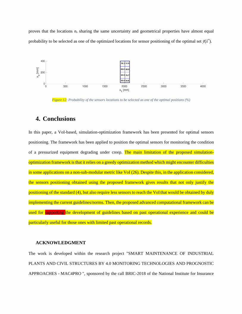
proves that the locations ns sharing the same uncertainty and geometrical properties have almost equal

probability to be selected as one of the optimized locations for sensor positioning of the optimal set y(x*).

Figure 12: Probability of the sensors locations to be selected as one of the optimal positions (%)

4. Conclusions

In this paper, a VoI-based, simulation-optimization framework has been presented for optimal sensors

positioning. The framework has been applied to position the optimal sensors for monitoring the condition

of a pressurized equipment degrading under creep. The main limitation of the proposed simulation-

optimization framework is that it relies on a greedy optimization method which might encounter difficulties

in some applications on a non-sub-modular metric like VoI (26). Despite this, in the application considered,

the sensors positioning obtained using the proposed framework gives results that not only justify the

positioning of the standard (4), but also require less sensors to reach the VoI that would be obtained by duly

implementing the current guidelines/norms. Then, the proposed advanced computational framework can be

used for supporting the development of guidelines based on past operational experience and could be

particularly useful for those ones with limited past operational records.

ACKNOWLEDGMENT

The work is developed within the research project "SMART MAINTENANCE OF INDUSTRIAL

PLANTS AND CIVIL STRUCTURES BY 4.0 MONITORING TECHNOLOGIES AND PROGNOSTIC

APPROACHES - MAC4PRO ", sponsored by the call BRIC-2018 of the National Institute for Insurance

against Accidents at Work – INAIL (CUP: J56C18002030001).

REFERENCES

1. Jelwan J, Chowdhury M, Pearce G. Creep life design criterion and its applications to pressure vessel

codes. Materials Physics and Mechanics. 2011; 11(2): p. 157-182.

2. Stewart M. 2 - Piping standards, codes, and recommended practices. In Surface Production

Operations: Volume 3: Facility Piping and Pipeline System.: Gulf Professional Publishing; 2016. p.

17-158.

3. Drummond MF. Introduction: the rationale for guidelines. Drug Information Journal. 1996; 30(2): p.

491-493.

4. UNI 11096. Non destructive testing - Structural integrity inspection of pressure equipment under

creep condition - Inspection planning and execution, results evaluation and report. Rome:; 2012.

5. EN 13445. Unfired pressure vessels. ; 2018.

6. ASME. Boiler and Pressure Vessel Code. ; 2017.

7. Auerkari P, Brown TB, Holdsworth S, Hales R, Klenk A, Patel R, et al. Developments in assessing

creep behaviour and creep life of components. Materials at High Temperatures \. 2004; 21(1): p. 61-

64.

8. Delle Site C, Petris CD, Mennuti C. NDT tools for life assessment of high temperature pressure

components. In ; 2006; Berlin, Germany: Proc. 9th European NDT (ECNDT) Conf.

9. Sposito G,WC, Cawley P, Nagy PB, Scruby C. A review of non-destructive techniques for the

detection of creep damage in power plant steels. Ndt & E International. 2010; 43(7): p. 555-567.

10. Baylac G, Kiesewetter N, Zeman J, Handtschoewercker A, McFarlane R, Corrado DS, et al. Creep

Amendments in the European Standard EN 13445. In ; 2007: ASME 2007 Pressure Vessels and

Piping Conference, pp.

11. Jaske CE, Topalis P, Loong WS, Sidek ASM. Risk Based Inspection Methodology for Components

Subject to High-Temperature Creep. In ; 2017: ASME 2017 Pressure Vessels and Piping

Conference.

12. Fong JT,N, Heckert A, Filliben JJ, Freiman. SW. A multi-scale failure-probability-based fatigue or

creep rupture life model for estimating component co-reliability. International Journal of Pressure

Vessels and Piping. 2019; 173 : p. 79-93.

13. Kumar A, Mathuriya S, Shilpi S. Detection of Creep Damage and Fatigue Failure in Thermal Power

Plants and Pipelines by Non-Destructive Testing Techniques. A Review. International journal of

engineering research and technology. 2014.

14. Tonti A, Site CD, Grisolia O, Franchi E. Italian Life-Assessment Procedure for Creep-Operated

Pressure Equipment. In ; 2007; American Society of Mechanical Engineers.: ASME 2007 Pressure

Vessels and Piping Conference. p. 535-540.

15. Faber MH. Risk and safety in civil engineering Zurich: Swiss Federal Institute of Technology ETH;

2007.

16. Daga R, Samal MK. Real-time monitoring of high temperature components. Procedia Engineering.

2013; 55: p. 421-427.

17. Rao GN. In-service inspection and structural health monitoring for safe and reliable operation of

NPPs. Procedia Engineering. 2014; 86: p. 476-485.

18. Noteboom JW, Hulshof HJM. On stream optical measurement to monitor creep strain. In ; 2017;

London; United Kingdom: WCCM 2017 - 1st World Congress on Condition Monitoring.

19. Zio E. The future of risk assessment. Reliability Engineering & System Safety. 2018; 177 : p. 176-

190.

20. DeGroot MH. Optimal statistical decisions Vol. 82: ohn Wiley & Sons; 2005.

21. Raiffa H, Schlaifer R. Applied Statistical Decision Theory: Harvard University; 1961.

22. Straub D. Value of information analysis with structural reliability methods. Structural Safety. 2014;

49 : p. 75-85.

23. Haladuick S, Dann. MR. Value of information-based decision analysis of the optimal next inspection

type for deteriorating structural systems. Structure and Infrastructure Engineering. 2018; 14(9): p.

1283-1292.

24. Malings C, Pozzi M. Value of Information for Spatially Distributed Systems: application to sensor

placement. Reliability Engineering & System Safety. 2016a; 154: p. 219-233.

25. Malings C, Pozzi M. Submodularity issues in value-of-information-based sensor placement.

Reliability Engineering & System Safety. 2019; 183 : p. 93-103.

26. Hoseyni SM, Maio FD, E. Zio. VoI-Based Optimal Sensors Positioning and the Sub-Modularity

Issue. In ; 2019; Rome, Italy: 4th International Conference on System Reliability and Safety

(ICSRS), pp. 148-152.

27. Kocijan J. Modelling and control of dynamic systems using Gaussian process models: Springer

International Publishing; 2016.

28. Malings C, Pozzi M. Value-of-information in spatio-temporal systems: Sensor placement and

scheduling. Reliability Engineering & System Safety. 2018; 172: p. 45-57.

29. Valls Miro J, Ulapane N, Shi L, Hunt D, Behrens M. Robotic pipeline wall thickness evaluation for

dense nondestructive testing inspection. Journal of Field Robotics. 2018; 35(8): p. 1293-1310.

30. Svensson A, Solin A, Särkkä S, Schön T. Computationally efficient Bayesian learning of Gaussian

process state space models. In ; 2016: Artificial Intelligence and Statistics (pp. 213-221).

31. Murphy KP. Conjugate Bayesian analysis of the Gaussian distribution. Vancouver:; 2007.

32. Di Maio F, Hoseyni SM, Zio E. Stima adattativa del rischio di rottura di componenti in pressione

soggetti a creep con un approccio probabilistico. In ; 2018; Bologna: SAFAP 2018-Sicurezza ed

affidabilità delle attrezzature a pressione.

33. ISPESL. Technical Procedure Concerning Calculation and Tests to Act on Creep-Operated Pressure

Vessel Components Circular N.48/2003, technical procedure issued in Italian. Italy:; 2003.

34. NIMS. NIMS Atlas of creep deformation property. No. D-1, Creep deformation properties of

9Cr1MoVNb steel for boiler and heat exchangers. Tokyo:; 2007.

35. Storesund J, Samuelson L, Klasen B. Creep life assessment of pipe girth weld repairs with

recommendations. OMMI. 2002; 1(3).