OPTIMAL SELECTION OF SENSORS AND

CONTROLLER PARAMETERS FOR ECONOMIC

OPTIMIZATION OF PROCESS PLANTS

A THESIS

submitted by

M. NABIL

for the award of the degree

of

DOCTOR OF PHILOSOPHY

DEPARTMENT OF CHEMICAL ENGINEERINGINDIAN INSTITUTE OF TECHNOLOGY MADRAS

SEPTEMBER 2014

THESIS CERTIFICATE

This is to certify that the thesis titled OPTIMAL SELECTION OF SENSORS AND

CONTROLLER PARAMETERS FOR ECONOMIC OPTIMIZATION OF PRO-

CESS PLANTS, submitted by M. NABIL, to the Indian Institute of Technology, Madras,

for the award of the degree of DOCTOR OF PHILOSOPHY, is a bonafide record of

the research work done by him under our supervision. The contents of this thesis, in full

or in parts, have not been submitted to any other Institute or University for the award of

any degree or diploma.

Dr. Sridharakumar NarasimhanResearch GuideAssociate ProfessorDept. of Chemical EngineeringIIT-Madras, 600 036

Place: Chennai

Date: 17th September 2014

To my parents

த ொடடனைத தூறும மணறகேணி மொந ரககுகககேறறனைததூறும அறிவு

- ிருககுகறள (396)

நுணணிய நூலபல ேறபினும மறறுந னஉணனம யறிகே மிுகம

- ிருககுகறள (373)

In sandy soil, when deep you delve, you reach the springs below;The more you learn, the freer streams of wisdom flow.

- G. U. Pope’s Translation of Thirukkural (396)

த ொடடனைத தூறும மணறகேணி மொந ரககுகககேறறனைததூறும அறிவு

- ிருககுகறள (396)

நுணணிய நூலபல ேறபினும மறறுந னஉணனம யறிகே மிுகம

- ிருககுகறள (373)

In subtle learning manifold though versed man be,’The wisdom, truly his, will gain supremacy.

- G. U. Pope’s Translation of Thirukkural (373)

ii

ACKNOWLEDGEMENTS

First of all, I am highly indebted to my supervisor Dr. Sridharakumar Narasimhan for

his unconditional care and affection. I express my sincere gratitude towards him for

his invaluable guidance and motivation throughout my PhD. My special thanks for his

continuous encouragement to attend conferences and summer schools. I also thank him

for giving me an opportunity to have an international exposure during my PhD.

I am grateful to Prof. Sigurd Skogestad for hosting me at NTNU and providing

invaluable and tireless guidance during nine months of stay in Norway. It was a great

learning experience both technically and socially. This thesis would not have taken this

shape without my stay over there.

My heartfelt thanks to Prof. Shankar Narasimhan, Prof. Raghunathan Rengaswamy

and Prof. Arun Tangirala, for the wonderful courses, constant support and good will.

All of them have made my understanding better and better by their priceless knowledge

and insightful comments during group meetings and DC meetings.

Dr. T. Renganathan has always been my source of motivation. Many a time, with-

out any reason, I have walked into CHL 210 or dialed 4186. I thank him for all his

love, guidance, friendship and good will. His research guidance during my M.Tech has

definitely played a significant role in my PhD.

Special thanks to Dr. Niket Kaisare for his invaluable career guidance.

I would like to thank Prof. Pushpavanam for the wonderful trips to Adventure zone

during his tenure as Head of the Department. I also thank him for the soft skills course

he arranged. I also thank Prof. Sreenivas Jayanthi for introducing interesting problems

in Transport phenomena.

I am thankful to office staffs Mrs. Regina, Mrs. Saraswati and Mr. Ravi for their

needful help.

Research at IITM would not have been better without the fun and friendship of

iii

Sudhakar, Anandhan, Arun, Keerthivasan, Gokul, Kathir, Abhishankar, Arun Sridha-

ran, Ayush, Danny, Hemanth, Venky, KJ, Bala, Sathish, Abhishek, Rahul, Raja Ashok,

Keerthiga, Rajmohan, ..., endless. They made special moments which I will cherish

forever.

I would like to thank my friends in Norway: Naresh, Rampa, Deepthanshu, Maryum,

Johannnes, Vinicius, Vlad, Chris, Mayil, Giri and Srikanth for making my stay most en-

joyable. My special thanks to Mr. Koneswaran for his kindness and love. I also thank

Mr. Aravazhi and Mr. Selva for their support.

I thank Govind for proof reading some parts of my thesis.

Special thanks to Mrs. Gowri and Mrs. Vaishnavi for the food they served whenever

mess had become messy. I thank Mrs. Gowri also for her friendship, joyful discussions

and care.

I thank Mani, Sathiyaraj, Naviyn and Deepak for their friendship.

I wouldn’t have come this far without the love and affection of my Late mother

Mumtaj, and hardwork of my father. I thank my brother Nizar for his helpful advices,

midnight skype calls, etc. I thank my sister, aunts and in-laws for their support at all

times.

I thank IIT Madras for funding my work. I thank the Research council of Norway

for funding nine months of my stay at NTNU, Trondheim. I would like to thank the De-

partment of Science and Technology, India for providing financial assistance to attend

the European Control Conference 2013, held at ETH Zurich. I also thank the Pacific

Institute of Mathematical Sciences, University of Calgary, and the IIT Madras Alumini

Association, for providing financial aid to attend 2013 summer school on optimization,

held at Calgary.

iv

ABSTRACT

KEYWORDS: optimal operation; measurement selection; set point selection; dy-

namic back-off; convex optimization; linear matrix inequality;

semi-definite programming; model predictive control.

In a typical chemical plant, the economic performance depends on several structural

and parametric decisions of the process. In order to quantify the economic performance,

we define the departure or loss function that measures the deviation from the optimal

cost, caused because of uncertainties. In this thesis, we particularly focus on making

a rational choice in the selection of measurements (structural decision), set points and

controller design (parametric decisions) based on the loss function. For this purpose,

we classify the relevant problems based on the nominal optimal point which is generally

obtained by minimizing the economic cost function subject to steady state model of the

process.

Firstly, if the nominal optimal solution is either unconstrained or constrained but

perfectly controllable, and there exists some unconstrained degrees of freedom, then

we focus on the measurement selection problem. It deals with determining the sen-

sor network by minimizing the loss function caused because of random measurement

errors. The main contributions along these lines include: (a) an analytical expression

that quantifies the economic loss caused due to measurement uncertainty is shown to

be sum of weighted error variances and an optimization problem that minimizes this

loss function is posed as an Mixed Integer Conic Problem (MICP) which can be solved

for globally optimal sensor network, (b) an optimization framework for determining

the best sensor network that can minimize the average loss and overall error in lexico-

graphic sense is proposed, and (c) an optimization formulation that finds the best set of

measurements that are robust to sensor failure situations by ensuring a certain level of

estimability of the network is presented.

v

Secondly, if the nominal optimal point is constrained but not perfectly controllable,

then we focus on the set point selection problem. It deals with finding a new profitable

operating point (i.e., backed-off point) that is also dynamically feasible in the presence

of uncertainties. The main contributions along these lines include: (a) assuming distur-

bances as the only source of uncertainty, we propose a novel two-stage iterative solution

algorithm to determine the economically optimal backed-off point when there is no con-

troller and in the presence of linear multivariable controller, (b) assuming measurement

errors as an addition source of uncertainty, the methodology is extended to find the best

set of measurements that will reduce the amount of back-off caused by measurement

errors in addition to controller design, and (c) for the case with disturbances only, the

practical implementation of the obtained multivariable controller using Model Predic-

tive Control (MPC) framework is studied by transforming the controller solution into

equivalent MPC weights.

vi

TABLE OF CONTENTS

ACKNOWLEDGEMENTS iii

ABSTRACT v

LIST OF TABLES xi

LIST OF FIGURES xiii

ABBREVIATIONS xv

NOTATION xvii

1 INTRODUCTION 1

1.1 Introduction . . . . . . . . . . . . . . . . . . . . . . . . . . . . . . 1

1.2 Motivation . . . . . . . . . . . . . . . . . . . . . . . . . . . . . . . 3

1.3 Optimal operation . . . . . . . . . . . . . . . . . . . . . . . . . . . 5

1.4 Mathematical framework . . . . . . . . . . . . . . . . . . . . . . . 8

1.4.1 Conic programming . . . . . . . . . . . . . . . . . . . . . 8

1.5 Research objectives . . . . . . . . . . . . . . . . . . . . . . . . . . 10

1.6 Thesis outline . . . . . . . . . . . . . . . . . . . . . . . . . . . . . 11

2 SENSOR NETWORK DESIGN 13

2.1 Background . . . . . . . . . . . . . . . . . . . . . . . . . . . . . . 13

2.2 Preliminaries . . . . . . . . . . . . . . . . . . . . . . . . . . . . . 17

2.3 Data Reconciliation (DR) . . . . . . . . . . . . . . . . . . . . . . . 18

2.3.1 Formulation 1 (Constrained DR problem) . . . . . . . . . . 19

2.3.2 Formulation 2 (Unconstrained DR problem) . . . . . . . . . 20

2.4 Sensor Network Design (SND) . . . . . . . . . . . . . . . . . . . . 23

2.4.1 Formulation 3 (SND based on overall error) . . . . . . . . . 23

2.4.2 SDP reformulation . . . . . . . . . . . . . . . . . . . . . . 24

vii

2.4.3 Illustration: Simple ammonia process . . . . . . . . . . . . 26

2.5 Summary . . . . . . . . . . . . . . . . . . . . . . . . . . . . . . . 27

3 SENSOR NETWORK DESIGN FOR OPTIMAL PROCESS OPERA-TIONS 29

3.1 Sensor network design for optimal operation . . . . . . . . . . . . . 31

3.1.1 Problem formulation . . . . . . . . . . . . . . . . . . . . . 31

3.1.2 Mixed Integer Cone Program (MICP) . . . . . . . . . . . . 36

3.1.3 Illustration 1: Simple ammonia process . . . . . . . . . . . 38

3.1.4 Illustration 2: Evaporation process . . . . . . . . . . . . . . 40

3.1.5 Computational issues . . . . . . . . . . . . . . . . . . . . . 45

3.2 Lexicographic optimization . . . . . . . . . . . . . . . . . . . . . . 46

3.2.1 Illustration: Simple ammonia process . . . . . . . . . . . . 49

3.3 Summary . . . . . . . . . . . . . . . . . . . . . . . . . . . . . . . 50

4 ROBUST OPTIMAL SENSOR NETWORK DESIGN 51

4.1 Introduction . . . . . . . . . . . . . . . . . . . . . . . . . . . . . . 51

4.2 Robust optimal sensor network design: Average loss formulation . . 52

4.2.1 Illustration: Evaporation process . . . . . . . . . . . . . . . 57

4.3 Robust optimal sensor network design: Worst-case average loss formu-lation . . . . . . . . . . . . . . . . . . . . . . . . . . . . . . . . . 59

4.3.1 Illustration: Evaporation process . . . . . . . . . . . . . . . 60

4.4 Summary . . . . . . . . . . . . . . . . . . . . . . . . . . . . . . . 61

5 PROFITABLE AND DYNAMICALLY FEASIBLE OPERATING POINTSELECTION FOR CONSTRAINED PROCESSES 63

5.1 Introduction . . . . . . . . . . . . . . . . . . . . . . . . . . . . . . 63

5.2 Formulation of dynamic back-off problem . . . . . . . . . . . . . . 67

5.2.1 Optimization formulation . . . . . . . . . . . . . . . . . . 67

5.2.2 Stochastic framework . . . . . . . . . . . . . . . . . . . . . 71

5.2.3 Convex relaxations . . . . . . . . . . . . . . . . . . . . . . 73

5.3 Solution methodology . . . . . . . . . . . . . . . . . . . . . . . . . 76

5.3.1 Stage 1 . . . . . . . . . . . . . . . . . . . . . . . . . . . . 77

5.3.2 Stage 2 . . . . . . . . . . . . . . . . . . . . . . . . . . . . 79

viii

5.4 Illustrations . . . . . . . . . . . . . . . . . . . . . . . . . . . . . . 80

5.4.1 Mass spring damper system . . . . . . . . . . . . . . . . . 80

5.4.2 Preheating furnace reactor system . . . . . . . . . . . . . . 83

5.4.3 Evaporation process . . . . . . . . . . . . . . . . . . . . . 85

5.5 Summary . . . . . . . . . . . . . . . . . . . . . . . . . . . . . . . 93

6 ECONOMIC PERFORMANCE OF MODEL PREDICTIVE CONTROLFOR CONSTRAINED PROCESSES 95

6.1 Introduction . . . . . . . . . . . . . . . . . . . . . . . . . . . . . . 95

6.2 Standard MPC vs Economic MPC . . . . . . . . . . . . . . . . . . 98

6.3 Target selection using economic back-off approach . . . . . . . . . 102

6.3.1 Problem formulation . . . . . . . . . . . . . . . . . . . . . 102

6.3.2 Solution methodology . . . . . . . . . . . . . . . . . . . . 105

6.4 MPC regulation at economic back-off point . . . . . . . . . . . . . 108

6.5 Illustrations . . . . . . . . . . . . . . . . . . . . . . . . . . . . . . 110

6.5.1 Mass spring damper system . . . . . . . . . . . . . . . . . 110

6.5.2 Evaporation process . . . . . . . . . . . . . . . . . . . . . 112

6.6 Summary . . . . . . . . . . . . . . . . . . . . . . . . . . . . . . . 117

7 SIMULTANEOUS SELECTION OF BACKED-OFF OPERATING POINT,CONTROLLER AND MEASUREMENTS BASED ON ECONOMICS 119

7.1 Introduction . . . . . . . . . . . . . . . . . . . . . . . . . . . . . . 119

7.2 Problem formulation . . . . . . . . . . . . . . . . . . . . . . . . . 120

7.2.1 Economic back-off . . . . . . . . . . . . . . . . . . . . . . 120

7.2.2 Sensor placement . . . . . . . . . . . . . . . . . . . . . . . 122

7.3 Solution methodology . . . . . . . . . . . . . . . . . . . . . . . . . 124

7.3.1 Stage 1 . . . . . . . . . . . . . . . . . . . . . . . . . . . . 125

7.3.2 Stage 2 . . . . . . . . . . . . . . . . . . . . . . . . . . . . 125

7.4 Illustration: Evaporation process . . . . . . . . . . . . . . . . . . . 126

7.5 Summary . . . . . . . . . . . . . . . . . . . . . . . . . . . . . . . 130

8 CONCLUSIONS AND RECOMMENDATIONS 131

8.1 Conclusions . . . . . . . . . . . . . . . . . . . . . . . . . . . . . . 131

ix

8.2 Recommendations . . . . . . . . . . . . . . . . . . . . . . . . . . . 133

A DERIVATION OF Equation 2.13 135

x

LIST OF TABLES

3.1 Comparison of average loss and overall error of a simple ammonia pro-cess . . . . . . . . . . . . . . . . . . . . . . . . . . . . . . . . . . 39

3.2 Variables and their nominal optimal values of the evaporation process 42

3.3 Comparison of average loss and overall error of the evaporation processfor some representative sensor networks . . . . . . . . . . . . . . . 45

3.4 Best additional sensor for a given network of the evaporation process 46

3.5 Computational efficiency of the proposed MICP approach . . . . . . 46

4.1 Redundant sensor selection of the evaporation process given differentbudget limits . . . . . . . . . . . . . . . . . . . . . . . . . . . . . 58

4.2 Robust optimal sensor networks of the evaporation process given dif-ferent budget limits . . . . . . . . . . . . . . . . . . . . . . . . . . 58

4.3 Optimal worst-case average loss value of the robust sensor network ofthe evaporation process given different budget limits . . . . . . . . 61

5.1 Algorithm for selecting economic back-off operating point . . . . . 80

5.2 EBOP values for change in constraint polytope of mass spring dampersystem . . . . . . . . . . . . . . . . . . . . . . . . . . . . . . . . . 82

5.3 Nominal values and EBOP solution of the preheater furnace reactorsystem . . . . . . . . . . . . . . . . . . . . . . . . . . . . . . . . . 85

5.4 Variables and nominal optimal values of the evaporation process . . 89

5.5 Nominal values and EBOP solution of the evaporator system . . . . 91

5.6 Computational efficiency of the proposed EBOP algorithm . . . . . 93

6.1 Algorithm for selecting economic back-off operating point for discretetime process . . . . . . . . . . . . . . . . . . . . . . . . . . . . . . 107

6.2 Nominal values and backed-off operating point of the evaporation pro-cess . . . . . . . . . . . . . . . . . . . . . . . . . . . . . . . . . . 113

7.1 Comparison of backed-off solutions of evaporation process for FSI andPSI cases . . . . . . . . . . . . . . . . . . . . . . . . . . . . . . . 128

7.2 Sensor network design of evaporation process operated at backed-offoperating point . . . . . . . . . . . . . . . . . . . . . . . . . . . . 128

xi

LIST OF FIGURES

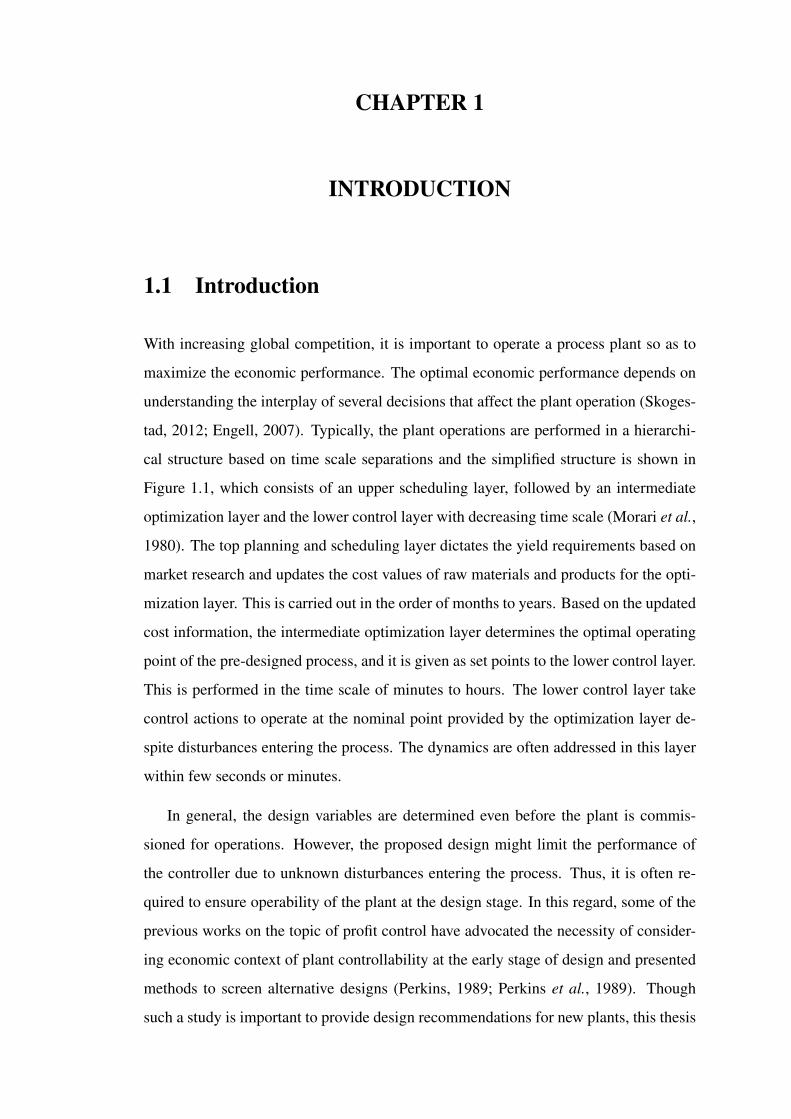
1.1 Hierarchical structure of plant operations based on time scale separationshowing the set of decisions involved in optimization and control layer 2

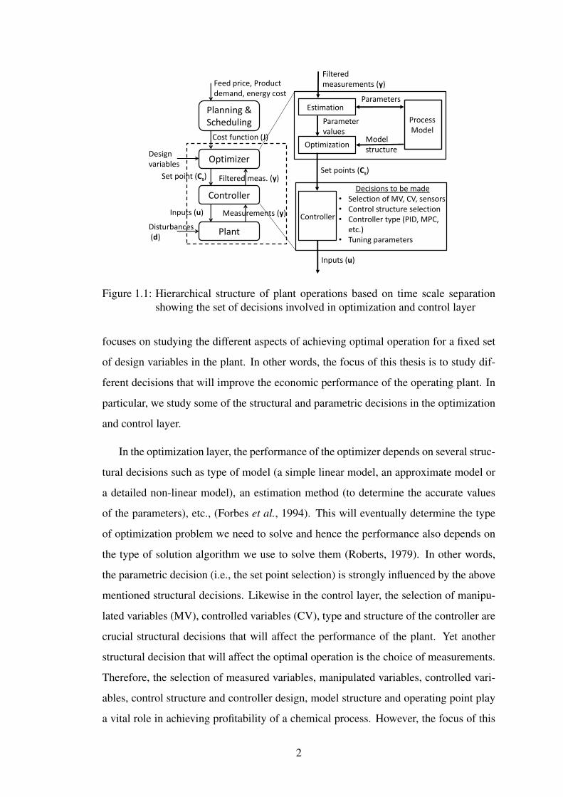
1.2 Set point selection showing performance of - (a) a badly tuned linearcontroller, (b) a well tuned linear controller, and (c) a well tuned non-linear controller . . . . . . . . . . . . . . . . . . . . . . . . . . . . 4

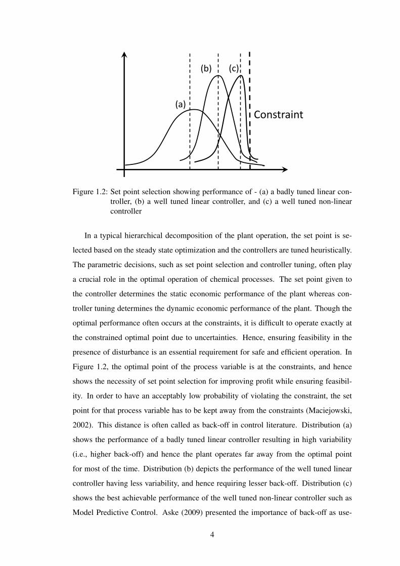
1.3 Nature of optimal solutions - unconstrained; partially constrained; fullyconstrained optimum . . . . . . . . . . . . . . . . . . . . . . . . . 6

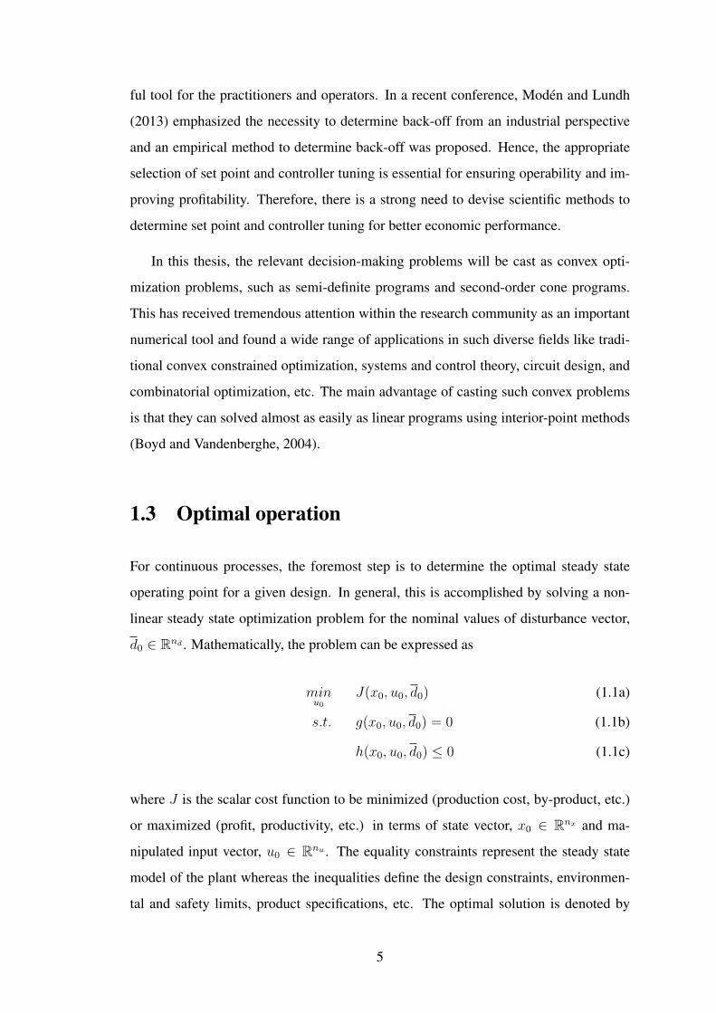
1.4 Process operation under uncertain conditions in input-output space atunconstrained and constrained optimum . . . . . . . . . . . . . . . 7

1.5 Roadmap of this thesis . . . . . . . . . . . . . . . . . . . . . . . . 12

2.1 Concept of observable and redundant sensor network . . . . . . . . 18

2.2 Splitter unit . . . . . . . . . . . . . . . . . . . . . . . . . . . . . . 21

2.3 Simple ammonia process . . . . . . . . . . . . . . . . . . . . . . . 26

3.1 Evaporator system . . . . . . . . . . . . . . . . . . . . . . . . . . . 40

4.1 Concept of robust sensor network . . . . . . . . . . . . . . . . . . 54

5.1 Feasible region: dynamic (box) and steady state (dashed line). . . . 68

5.2 Non-optimal controller design (solution from Stage 1) . . . . . . . . 77

5.3 Optimal controller design (after convergence) . . . . . . . . . . . . 78

5.4 Mass spring damper system . . . . . . . . . . . . . . . . . . . . . . 81

5.5 Impact of change in constraint for mass spring damper system . . . 82

5.6 Preheating furnace reactor system . . . . . . . . . . . . . . . . . . 83

5.7 Furnace temperature vs reactor temperature . . . . . . . . . . . . . 86

5.8 Furnace temperature vs feed flow rate . . . . . . . . . . . . . . . . 86

5.9 Furnace temperature vs fuel flow rate . . . . . . . . . . . . . . . . . 87

5.10 Furnace temperature vs O2 concentration . . . . . . . . . . . . . . 87

5.11 Furnace temperature vs CO concentration . . . . . . . . . . . . . . 88

5.12 Furnace temperature vs vent position . . . . . . . . . . . . . . . . . 88

xiii

5.13 Evaporator system . . . . . . . . . . . . . . . . . . . . . . . . . . . 89

5.14 Product composition vs operating pressure. a) Open loop case: F3 andF200 are constant. b) Closed loop case: F3 and F200 are used for controlof X2 . . . . . . . . . . . . . . . . . . . . . . . . . . . . . . . . . 90

5.15 Product composition vs recirculation flow rate . . . . . . . . . . . . 90

5.16 Product composition vs steam pressure . . . . . . . . . . . . . . . . 91

5.17 Product composition vs coolant flow rate . . . . . . . . . . . . . . . 91

6.1 Two stage iterative solution approach for economic back-off selection:(a) stage 1 solution; (b) stage 2 solution; (c) converged stage 2 solution 106

6.2 Scatter plot of a mass spring damper system showing the performanceof multivariable controller, uk = Ldxk . . . . . . . . . . . . . . . . 111

6.3 Scatter plot of a mass spring damper system showing the performanceof MPC controller . . . . . . . . . . . . . . . . . . . . . . . . . . . 111

6.4 Time series plot of a mass spring damper system showing the perfor-mance of multivariable controller, uk = Ldxk . . . . . . . . . . . . 112

6.5 Time series plot a mass spring damper system showing the performanceof MPC controller . . . . . . . . . . . . . . . . . . . . . . . . . . . 112

6.6 Scatter plot showing the EDOR between product composition vs oper-ating pressure . . . . . . . . . . . . . . . . . . . . . . . . . . . . . 113

6.7 Scatter plot showing the EDOR between product composition vs recir-culation flow rate . . . . . . . . . . . . . . . . . . . . . . . . . . . 114

6.8 Scatter plot showing the EDOR between product composition vs steampressure . . . . . . . . . . . . . . . . . . . . . . . . . . . . . . . . 114

6.9 Scatter plot showing the EDOR between product composition vs coolantflow rate . . . . . . . . . . . . . . . . . . . . . . . . . . . . . . . . 114

6.10 Time-series plot of the evaporation process showing the controller per-formances at the economic back-off point . . . . . . . . . . . . . . 115

7.1 Product composition vs operating pressure. a) Continuous line : FSIcase b) Dashed line : PSI case . . . . . . . . . . . . . . . . . . . . 127

7.2 Product composition vs recirculation flow rate . . . . . . . . . . . . 127

7.3 Product composition vs steam pressure . . . . . . . . . . . . . . . . 127

7.4 Product composition vs coolant flow rate . . . . . . . . . . . . . . . 128

xiv

ABBREVIATIONS

BOP Backed-off Operating Point

CV Controlled Variables

DR Data Reconciliation

EBOP Economic Backed-off Operating Point

EDOR Expected Dynamic Operating Region

EVO Engineering Virtual Organization

FSI Full State Information

LMI Linear Matrix Inequality

LP Linear Programming

MICP Mixed Integer Cone Programming

MILP Mixed Integer Linear Programming

MINLP Mixed Integer Non-Linear Programming

MPC Model Predictive Control

MV Manipulated Variables

OOP Optimal Operating Point

PI Proportional-Integral

PID Proportional-Integral-Derivative

PSI Partial State Information

SDP Semi-Definite Programming

SND Sensor Network Design

SOC Second Order Cone

xv

NOTATION

English alphabetsA,Ad system matrices of a continuous time and discrete time state space modelA1, A2 columns of A in the linear process model Ax = 0, corresponding to

measured and unmeasured variablesAp, As columns of A in the linear process model Ax = 0, corresponding to

primary and secondary variablesB,Bd system matrices of a continuous time and discrete time state space modelC process matrixci cost of the sensor for measuring variable zic∗ budget limit for purchasing sensorsd disturbance variablesG,Gd system matrices of a continuous time and discrete time state space modelJ negated profit functionk number of sensors to be selectedL controller gain matrix in u = LxL operational loss due to measurement errors` stage cost in MPCM parameter in the lexicographic formulationNmin minimum number of sensorsn total number of variablesna number of active constrained variablesnd number of disturbance variablesne number of model equationsnu number of manipulated variablesnuc,dof number of unconstrained degrees of freedomnx number of state variablesny number of measurementsqi binary decision variable denoting the presence or absense of a sensorQ diag( qi

σ2i) ; objective function weights in MPC

R objective function weights in MPCR set of real numbersR+ set of non negative real numbersR++ set of positive real numbersRn set of real n-vectorsRm×n set of real m× n matricesSF set of possible sensors that can fail at a timeSn set of symmetric n× n matricesSn+ set of symmetric positive semidefinite n× n matricesSn++ set of symmetric positive definite n× n matrices

xvii

u manipulated variablesvm error vectorW weighting matrix in the sensor network design formulation, W = RRT

x state variablesz vector of process variableszm measured variableszp primary variableszs secondary variableszu unmeasured variables

Greek alphabetsα prescribed confidence level∆u difference between the BOP value of u and its bound umin or umax∆x difference between the BOP value of x and its bound xmin or xmaxδi,j ratio of distance of variable i from its closest bound to the distance of

variable j from its closest boundεd error in disturbance variable dεu error in input variable uεx error in state variable xεz error in process variable zΣz error covariance matrix of the estimates zΣv diagonal covariance matrix of the error vector vmσi variance of the process variable ziΦ total stage cost in standard MPC formulationΦebop total stage cost in economic back-off based MPC formulationΦeco total stage cost in economic MPC formulationλ1, λ2 objective function weights of the lexicographic formulation

Operators||(.)|| norm of (.)diag(.) diagonalize (.)E[.] expectation of [.]g(.) process model functionsh(.) process constraint functions

Accents(.) estimate of (.)(.) nominal optimal value of (.)(.) deviation from the nominal optimal value (.)

Superscripts and subscriptste, Ye internal variables in overall estimation error formulationtc, Yc internal variables in average loss formulationx∗ optimal value of xxk value of x at time instant kxmax maximum value of xxmin minimum value of xxss steady state values of x

xviii

xix

CHAPTER 1

INTRODUCTION

1.1 Introduction

With increasing global competition, it is important to operate a process plant so as to

maximize the economic performance. The optimal economic performance depends on

understanding the interplay of several decisions that affect the plant operation (Skoges-

tad, 2012; Engell, 2007). Typically, the plant operations are performed in a hierarchi-

cal structure based on time scale separations and the simplified structure is shown in

Figure 1.1, which consists of an upper scheduling layer, followed by an intermediate

optimization layer and the lower control layer with decreasing time scale (Morari et al.,

1980). The top planning and scheduling layer dictates the yield requirements based on

market research and updates the cost values of raw materials and products for the opti-

mization layer. This is carried out in the order of months to years. Based on the updated

cost information, the intermediate optimization layer determines the optimal operating

point of the pre-designed process, and it is given as set points to the lower control layer.

This is performed in the time scale of minutes to hours. The lower control layer take

control actions to operate at the nominal point provided by the optimization layer de-

spite disturbances entering the process. The dynamics are often addressed in this layer

within few seconds or minutes.

In general, the design variables are determined even before the plant is commis-

sioned for operations. However, the proposed design might limit the performance of

the controller due to unknown disturbances entering the process. Thus, it is often re-

quired to ensure operability of the plant at the design stage. In this regard, some of the

previous works on the topic of profit control have advocated the necessity of consider-

ing economic context of plant controllability at the early stage of design and presented

methods to screen alternative designs (Perkins, 1989; Perkins et al., 1989). Though

such a study is important to provide design recommendations for new plants, this thesis

Plant

Controller

Optimizer

Planning & Scheduling

Design variables

Feed price, Product demand, energy cost

Cost function (J)

Set point (Cs)

Measurements (y)Inputs (u)

Disturbances(d)

Process Model

Parameters

Parameter values

Model structure

Estimation

Optimization

Set points (Cs)

Decisions to be made• Selection of MV, CV, sensors• Control structure selection• Controller type (PID, MPC,

etc.)• Tuning parameters

Filtered measurements (y)

Filtered meas. (y)

Inputs (u)

Controller

Figure 1.1: Hierarchical structure of plant operations based on time scale separationshowing the set of decisions involved in optimization and control layer

focuses on studying the different aspects of achieving optimal operation for a fixed set

of design variables in the plant. In other words, the focus of this thesis is to study dif-

ferent decisions that will improve the economic performance of the operating plant. In

particular, we study some of the structural and parametric decisions in the optimization

and control layer.

In the optimization layer, the performance of the optimizer depends on several struc-

tural decisions such as type of model (a simple linear model, an approximate model or

a detailed non-linear model), an estimation method (to determine the accurate values

of the parameters), etc., (Forbes et al., 1994). This will eventually determine the type

of optimization problem we need to solve and hence the performance also depends on

the type of solution algorithm we use to solve them (Roberts, 1979). In other words,

the parametric decision (i.e., the set point selection) is strongly influenced by the above

mentioned structural decisions. Likewise in the control layer, the selection of manipu-

lated variables (MV), controlled variables (CV), type and structure of the controller are

crucial structural decisions that will affect the performance of the plant. Yet another

structural decision that will affect the optimal operation is the choice of measurements.

Therefore, the selection of measured variables, manipulated variables, controlled vari-

ables, control structure and controller design, model structure and operating point play

a vital role in achieving profitability of a chemical process. However, the focus of this

2

thesis is limited to the selection of operating point (parametric decision) given the model

of the plant and structural decisions on the controller. We also focus on the selection of

measurements (structural decision) to improve economic benefits.

1.2 Motivation

In this thesis, we address two important problems viz., sensor network design and set

point selection along with controller tuning from a profit perspective. Efficient pro-

cess monitoring, control and fault diagnosis are vital for optimal and safe operation

of a chemical process. The success of each of the above activities depends critically

on the choice of the sensor network. Although sensor network design problems have

been discussed extensively in literature, they are tailored for each activity independently

(Chmielewski et al., 2002; Bhushan and Rengaswamy, 2000). Since the individual de-

sign problems are incommensurable, the integration of sensor network design is difficult

to account for the multi-faceted elements (observability, controllability, redundancy, ac-

curacy, reliability, etc.,). Several years ago, it was identified that sensor networks ought

to be designed so that plant performance is optimal from the profit perspective.

Recently, it has been highlighted by the Engineering Virtual Organization (EVO - a

consortium of leading US universities, automation industries and the US NSF), that the

optimal sensor network design for process plant is an important research issue. Specific

research challenges pertaining to the next-generation sensor network design has been

listed as (Davis, 2008):

• “Sensor network for plant status - Design sensor networks to improve plant ob-servability and bias free state estimation and control”

• “Network design for sensor/actuator-based control - Develop associated actuatorand sensor instrumentation networks for fault-tolerant control that is compatiblewith other functions such as quality control, production accounting and on-lineoptimization”

Therefore, it is necessary to define performance metrics based on process economics

for designing sensor networks within the integrated optimization and control frame-

work.

3

Constraint(a)

(b) (c)

Figure 1.2: Set point selection showing performance of - (a) a badly tuned linear con-troller, (b) a well tuned linear controller, and (c) a well tuned non-linearcontroller

In a typical hierarchical decomposition of the plant operation, the set point is se-

lected based on the steady state optimization and the controllers are tuned heuristically.

The parametric decisions, such as set point selection and controller tuning, often play

a crucial role in the optimal operation of chemical processes. The set point given to

the controller determines the static economic performance of the plant whereas con-

troller tuning determines the dynamic economic performance of the plant. Though the

optimal performance often occurs at the constraints, it is difficult to operate exactly at

the constrained optimal point due to uncertainties. Hence, ensuring feasibility in the

presence of disturbance is an essential requirement for safe and efficient operation. In

Figure 1.2, the optimal point of the process variable is at the constraints, and hence

shows the necessity of set point selection for improving profit while ensuring feasibil-

ity. In order to have an acceptably low probability of violating the constraint, the set

point for that process variable has to be kept away from the constraints (Maciejowski,

2002). This distance is often called as back-off in control literature. Distribution (a)

shows the performance of a badly tuned linear controller resulting in high variability

(i.e., higher back-off) and hence the plant operates far away from the optimal point

for most of the time. Distribution (b) depicts the performance of the well tuned linear

controller having less variability, and hence requiring lesser back-off. Distribution (c)

shows the best achievable performance of the well tuned non-linear controller such as

Model Predictive Control. Aske (2009) presented the importance of back-off as use-

4

ful tool for the practitioners and operators. In a recent conference, Modén and Lundh

(2013) emphasized the necessity to determine back-off from an industrial perspective

and an empirical method to determine back-off was proposed. Hence, the appropriate

selection of set point and controller tuning is essential for ensuring operability and im-

proving profitability. Therefore, there is a strong need to devise scientific methods to

determine set point and controller tuning for better economic performance.

In this thesis, the relevant decision-making problems will be cast as convex opti-

mization problems, such as semi-definite programs and second-order cone programs.

This has received tremendous attention within the research community as an important

numerical tool and found a wide range of applications in such diverse fields like tradi-

tional convex constrained optimization, systems and control theory, circuit design, and

combinatorial optimization, etc. The main advantage of casting such convex problems

is that they can solved almost as easily as linear programs using interior-point methods

(Boyd and Vandenberghe, 2004).

1.3 Optimal operation

For continuous processes, the foremost step is to determine the optimal steady state

operating point for a given design. In general, this is accomplished by solving a non-

linear steady state optimization problem for the nominal values of disturbance vector,

d0 ∈ Rnd . Mathematically, the problem can be expressed as

minu0

J(x0, u0, d0) (1.1a)

s.t. g(x0, u0, d0) = 0 (1.1b)

h(x0, u0, d0) ≤ 0 (1.1c)

where J is the scalar cost function to be minimized (production cost, by-product, etc.)

or maximized (profit, productivity, etc.) in terms of state vector, x0 ∈ Rnx and ma-

nipulated input vector, u0 ∈ Rnu . The equality constraints represent the steady state

model of the plant whereas the inequalities define the design constraints, environmen-

tal and safety limits, product specifications, etc. The optimal solution is denoted by

5

DoF 1

Do

F2 Optimal

point

Constraints Optimalpoint

Constraints

Optimal point

Constraints

DoF 1 DoF 1

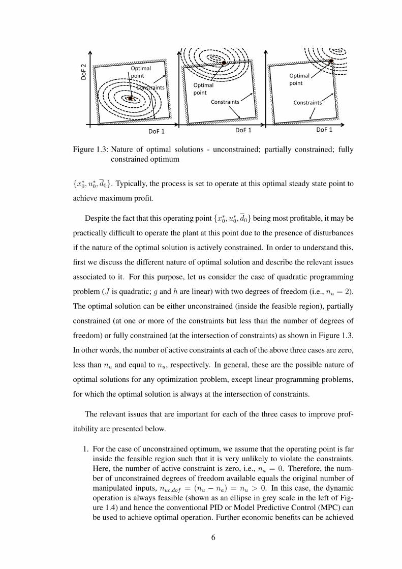
Figure 1.3: Nature of optimal solutions - unconstrained; partially constrained; fullyconstrained optimum

{x∗0, u∗0, d0}. Typically, the process is set to operate at this optimal steady state point to

achieve maximum profit.

Despite the fact that this operating point {x∗0, u∗0, d0} being most profitable, it may be

practically difficult to operate the plant at this point due to the presence of disturbances

if the nature of the optimal solution is actively constrained. In order to understand this,

first we discuss the different nature of optimal solution and describe the relevant issues

associated to it. For this purpose, let us consider the case of quadratic programming

problem (J is quadratic; g and h are linear) with two degrees of freedom (i.e., nu = 2).

The optimal solution can be either unconstrained (inside the feasible region), partially

constrained (at one or more of the constraints but less than the number of degrees of

freedom) or fully constrained (at the intersection of constraints) as shown in Figure 1.3.

In other words, the number of active constraints at each of the above three cases are zero,

less than nu and equal to nu, respectively. In general, these are the possible nature of

optimal solutions for any optimization problem, except linear programming problems,

for which the optimal solution is always at the intersection of constraints.

The relevant issues that are important for each of the three cases to improve prof-

itability are presented below.

1. For the case of unconstrained optimum, we assume that the operating point is farinside the feasible region such that it is very unlikely to violate the constraints.Here, the number of active constraint is zero, i.e., na = 0. Therefore, the num-ber of unconstrained degrees of freedom available equals the original number ofmanipulated inputs, nuc,dof = (nu − na) = nu > 0. In this case, the dynamicoperation is always feasible (shown as an ellipse in grey scale in the left of Fig-ure 1.4) and hence the conventional PID or Model Predictive Control (MPC) canbe used to achieve optimal operation. Further economic benefits can be achieved

6

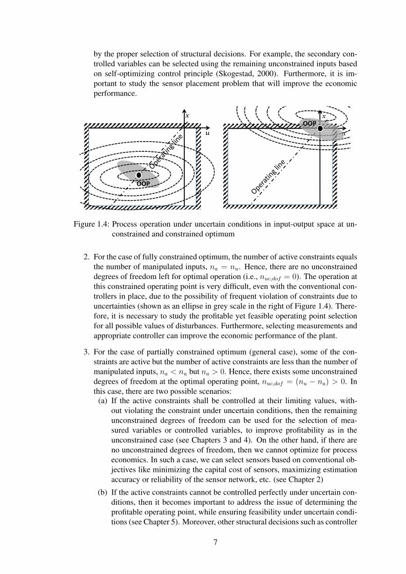
by the proper selection of structural decisions. For example, the secondary con-trolled variables can be selected using the remaining unconstrained inputs basedon self-optimizing control principle (Skogestad, 2000). Furthermore, it is im-portant to study the sensor placement problem that will improve the economicperformance.

OOP

OOP

Figure 1.4: Process operation under uncertain conditions in input-output space at un-constrained and constrained optimum

2. For the case of fully constrained optimum, the number of active constraints equalsthe number of manipulated inputs, na = nu. Hence, there are no unconstraineddegrees of freedom left for optimal operation (i.e., nuc,dof = 0). The operation atthis constrained operating point is very difficult, even with the conventional con-trollers in place, due to the possibility of frequent violation of constraints due touncertainties (shown as an ellipse in grey scale in the right of Figure 1.4). There-fore, it is necessary to study the profitable yet feasible operating point selectionfor all possible values of disturbances. Furthermore, selecting measurements andappropriate controller can improve the economic performance of the plant.

3. For the case of partially constrained optimum (general case), some of the con-straints are active but the number of active constraints are less than the number ofmanipulated inputs, na < nu but na > 0. Hence, there exists some unconstraineddegrees of freedom at the optimal operating point, nuc,dof = (nu − na) > 0. Inthis case, there are two possible scenarios:

(a) If the active constraints shall be controlled at their limiting values, with-out violating the constraint under uncertain conditions, then the remainingunconstrained degrees of freedom can be used for the selection of mea-sured variables or controlled variables, to improve profitability as in theunconstrained case (see Chapters 3 and 4). On the other hand, if there areno unconstrained degrees of freedom, then we cannot optimize for processeconomics. In such a case, we can select sensors based on conventional ob-jectives like minimizing the capital cost of sensors, maximizing estimationaccuracy or reliability of the sensor network, etc. (see Chapter 2)

(b) If the active constraints cannot be controlled perfectly under uncertain con-ditions, then it becomes important to address the issue of determining theprofitable operating point, while ensuring feasibility under uncertain condi-tions (see Chapter 5). Moreover, other structural decisions such as controller

7

design, measurement selection can also be considered (see Chapters 6 and7). This case is similar to fully constrained case.

In summary, our focus is two-fold: Firstly, we address the measurement selection

problem for the case of unconstrained or partially constrained nominal optimum with

unconstrained degrees of freedom and secondly, for the case of constrained nominal

optimum, we address the problem of set point selection such that it is both profitable

and feasible under uncertain conditions.

1.4 Mathematical framework

In this thesis, we cast the decision making process as optimization problems based

on strong theoretical foundations. Often, the parametric decisions (say for example,

selecting the set point or controller gain) and structural decisions (say for example, a

particular variable is being measured or not) are denoted by continuous and discrete

decision variables, respectively. In general, these problems are formulated as Mixed

Integer Non-Linear Programming (MINLP) problems, for which a candidate optimal

solution will guarantee only local optimum. Therefore, in this thesis, we primarily

work with conic programming problems which guarantees global optimality. Conic

solvers like SeDuMi or SDPT3 can be used under MATLAB to solve Semi-Definite

Programming (SDP) problems based on a polynomial-time interior-point method.

1.4.1 Conic programming

The aim of this section is to introduce the reader some of the basic definitions that

will be useful in understanding the optimization formulations presented in this thesis.

However, it is not meant to be an exhaustive treatment of the topic. For this, the reader

is referred to Vandenberghe and Boyd (1996), Alizadeh and Goldfarb (2003) and Anjos

and Lasserre (2012).

DEFINITION 1.1 A symmetric matrixX ∈ Sn is said to be positive definite, denoted

by X � 0, if

vTXv > 0 for all nonzero v ∈ Rn,

8

and positive semidefinite, denoted by X � 0, if

vTXv ≥ 0 for all v ∈ Rn.

DEFINITION 1.2 Let two points x, y ∈ Rn and 0 ≤ λ ≤ 1 be given. Then the point

z = λx+ (1− λ)y

is a convex combination of the two points x and y.

DEFINITION 1.3 The set C ⊂ Rn is called convex, if all convex combinations of

any two points x, y ∈ C are again in C.

DEFINITION 1.4 The set K ⊂ Rn is a convex cone if it is a convex set and for all

x ∈ K and λ > 0 we have λx ∈ K. A cone is called pointed if it does not contain any

subspace except the origin. A cone is said to be a proper cone if it is closed, convex and

pointed. The set of non-negative vectors Rn+ is an example of a proper cone.

DEFINITION 1.5 Second Order Cone (SOC) in Rn+1 can be expressed as

SOCn+1 := {(x, y) ∈ Rn+1|y ≥ ‖x‖2}

The SOC is another example of a proper cone.

DEFINITION 1.6 Linear Matrix Inequality (LMI) is an expression of the form,

F (x) = F0 + x1F1 + · · ·+ xmFm � 0

where the matrices Fi = F Ti ∈ Sn are given, and the inequality F (x) � 0 means

F (x) is positive semidefinite. The set of symmetric positive semidefinite matrices is

yet another example of a proper cone. Therefore, the LMI is a convex constraint in the

variable x ∈ Rm. Let X and Y be any symmetric matrices. We also write “X � Y ” to

denote that X − Y � 0.

Conic programming is a class of convex optimization problems which minimizes a

linear function (or possibly convex quadratic) function over the intersection of an affine

9

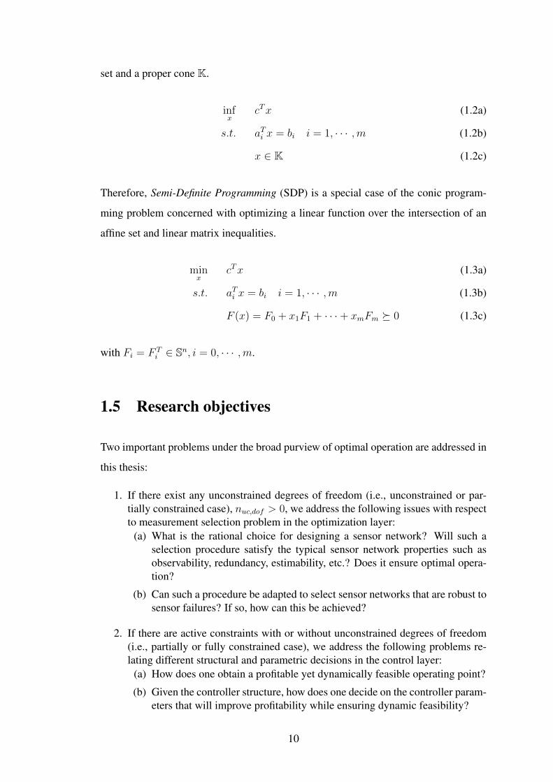
set and a proper cone K.

infx

cTx (1.2a)

s.t. aTi x = bi i = 1, · · · ,m (1.2b)

x ∈ K (1.2c)

Therefore, Semi-Definite Programming (SDP) is a special case of the conic program-

ming problem concerned with optimizing a linear function over the intersection of an

affine set and linear matrix inequalities.

minx

cTx (1.3a)

s.t. aTi x = bi i = 1, · · · ,m (1.3b)

F (x) = F0 + x1F1 + · · ·+ xmFm � 0 (1.3c)

with Fi = F Ti ∈ Sn, i = 0, · · · ,m.

1.5 Research objectives

Two important problems under the broad purview of optimal operation are addressed in

this thesis:

1. If there exist any unconstrained degrees of freedom (i.e., unconstrained or par-tially constrained case), nuc,dof > 0, we address the following issues with respectto measurement selection problem in the optimization layer:

(a) What is the rational choice for designing a sensor network? Will such aselection procedure satisfy the typical sensor network properties such asobservability, redundancy, estimability, etc.? Does it ensure optimal opera-tion?

(b) Can such a procedure be adapted to select sensor networks that are robust tosensor failures? If so, how can this be achieved?

2. If there are active constraints with or without unconstrained degrees of freedom(i.e., partially or fully constrained case), we address the following problems re-lating different structural and parametric decisions in the control layer:

(a) How does one obtain a profitable yet dynamically feasible operating point?

(b) Given the controller structure, how does one decide on the controller param-eters that will improve profitability while ensuring dynamic feasibility?

10

(c) How can this performance be obtained using Model Predictive Control (MPC),a widely used controller technique in the process industry.

(d) How does one identify the best set of measurements that will improve prof-itability?

1.6 Thesis outline

This thesis is organized as follows. Figure 1.5 presents the roadmap of this thesis.

• Chapter 2 presents the brief review of literatures on sensor network design. Next,we briefly describe the data reconciliation problem, followed by the sensor place-ment problem to obtain better reconciled estimates. In this chapter, we presentthe Mixed Integer Conic Programming (MICP) formulation for designing sensornetworks.

• In Chapter 3, we propose an average loss function based on the notion of op-erational profit to quantify the performance of sensor network in terms of lossincurred due to measurement errors. An optimization formulation is presented tofind a sensor network that minimizes the average loss. Using convex optimiza-tion theory, we cast the problem as an MICP, which could be solved for globaloptimality using existing branch and bound solvers.

• Chapter 4 extends the proposed sensor placement problem based on the averageloss function, to design reliable sensor networks that will be robust to sensor fail-ures. This is accomplished by designing redundant sensor networks such that, incase of sensor failures, the resultant subnetwork will be observable. Furthermore,we also modified the optimization formulation to determine the sensor networkthat minimizes the worst case loss in case of sensor failures.

• Chapter 5 is focused on determining the profitable yet dynamically feasible op-erating point selection for nominally constrained processes. In this chapter, wesurvey the relevant literatures and then present a back-off approach to circum-vent infeasible operations that could occur due to disturbances entering the pro-cess. Since backing off will result in an economic loss, we address the problemby optimizing the economic cost function subject to dynamic feasibility. Here,the amount of back-off is reduced by a suitable controller design. However, theresulting formulation is non-convex and hence we proposed a novel two stageiterative solution technique.

• In Chapter 6, we address the backed-off operating point selection problem usingdiscrete-time formulation for easy implementation using standard MPC frame-work. For this purpose, the designed linear multivariable controller is convertedto equivalent MPC weights and the economic performance of the process is stud-ied. Moreover, relevance to economic MPC is discussed.

• In Chapter 7, we extend the optimization formulation that was addressed for se-lecting economically backed-off operating point to include sensor selection. Here

11

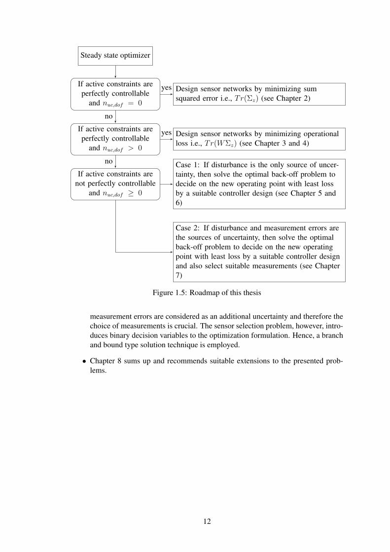
Steady state optimizer

If active constraints areperfectly controllable

and nuc,dof = 0

Design sensor networks by minimizing sumsquared error i.e., Tr(Σz) (see Chapter 2)

If active constraints areperfectly controllable

and nuc,dof > 0

Design sensor networks by minimizing operationalloss i.e., Tr(WΣz) (see Chapter 3 and 4)

If active constraints arenot perfectly controllable

and nuc,dof ≥ 0

Case 1: If disturbance is the only source of uncer-tainty, then solve the optimal back-off problem todecide on the new operating point with least lossby a suitable controller design (see Chapter 5 and6)

Case 2: If disturbance and measurement errors arethe sources of uncertainty, then solve the optimalback-off problem to decide on the new operatingpoint with least loss by a suitable controller designand also select suitable measurements (see Chapter7)

yes

no

yes

no

Figure 1.5: Roadmap of this thesis

measurement errors are considered as an additional uncertainty and therefore thechoice of measurements is crucial. The sensor selection problem, however, intro-duces binary decision variables to the optimization formulation. Hence, a branchand bound type solution technique is employed.

• Chapter 8 sums up and recommends suitable extensions to the presented prob-lems.

12

CHAPTER 2

SENSOR NETWORK DESIGN

In this chapter, we first briefly review the existing literatures on conventional sensor net-

work design procedures. For a particular case of perfectly controllable active constraints

with no unconstrained degrees of freedom, the structural decisions such as location of

sensors cannot affect the optimal operation. In such a case, the traditional sensor net-

work objectives like minimizing the instrumentation cost of the network, maximizing

the reliability of the network or maximizing the estimation accuracy of the network, etc.,

can be used. However, the optimization formulations will result in MINLPs, in general.

Therefore, the primary focus of this chapter is to present an SDP based optimization

formulation to design sensor networks that minimizes the estimation error.

2.1 Background

Sensors are the measuring elements of a process plant to infer the state of the process,

detect and diagnose faults, give feedback information to the controller, etc. Therefore,

the choice of a particular set of sensors plays a crucial role in the optimal operation

of a chemical process. The problem of sensor network design (also known as mea-

surement selection) has been widely studied in literature for several decades. However,

our literature survey presented here is limited in discussing the developments along the

following lines only: (a) First, we survey the different performance measures used in

quantifying sensor networks; (b) Next, we discuss the methods developed to handle

sensor failure situations, and (c) Finally, we discuss the computational algorithms that

have been developed to design sensor networks.

Typically, the problem of sensor network design uses some kind of sensor informa-

tion such as sensor cost, sensor variability, sensor failure probability, etc. and optimize

for some form of the network properties such as precision, reliability, instrumentation

cost, etc. while demanding some of the other properties like observability, redundancy,

resolvability, etc. being satisfied. In general, sensor network design procedures are

carried out to address a specific process activity and the performance measures were

defined specific to each activity. From the viewpoint of fault detection and diagnosis,

sensors are selected such that the faults are observable and resolvable. Ali (1993) in-

troduced the concept of reliability which uses the available sensor failure probability

information to quantify the network performance. In control applications, the problem

is usually that of selecting a suitable candidate set of controlled variables (Alstad et al.,

2009; Halvorsen et al., 2003). Given the set of measurements, data reconciliation pro-

cedures adjust the measurement so as to improve the estimation accuracy. From a data

reconciliation perspective, Kretsovalis and Mah (1987) adopted estimation accuracy as

a measure to choose sensor networks and also showed that adding redundant measure-

ments improved the estimation accuracy. For efficient process monitoring, a sensor

network should be capable of providing precise information about the state of the pro-

cess in the presence of random and gross errors. Traditional cost based approaches for

the design of sensor networks are primarily based on capital cost of the hardware ele-

ment. Bhushan and Rengaswamy (2002a,b) formulated an optimization problem that

minimizes the capital cost of sensors subject to reliability requirements and vice versa.

Specifications on precision, error detectability, resilience can be enforced as constraints

to obtain minimum cost networks (Bagajewicz, 1997; Bagajewicz and Sánchez, 2000;

Bagajewicz and Cabrera, 2002). Other cost factors such as maintenance cost for sen-

sors have been discussed by Nguyen and Bagajewicz (2009). Also, operational profit

based studies are increasingly important in recent years. Profit based metrics are eas-

ily decipherable and also of direct use to the end user. From a control viewpoint, Peng

and Chmielewski (2005) have developed a simultaneous formulation of sensor selection

and minimum backed - off operating point selection by maximizing the operating profit.

Likewise, the theory of self-optimizing control addresses the problem of selecting con-

trolled variables that results in a minimum operating loss (Alstad et al., 2009; Halvorsen

et al., 2003). Fraleigh et al. (2003) have developed expressions for the loss function

that quantifies the departure from optimality and have applied them to the sensor selec-

tion problem. On the other hand, Narasimhan and Rengaswamy (2007) addressed this

problem from a fault diagnostic perspective. Similar attempts have been made in the

reconciliation framework by Bagajewicz et al. (2005); Mazzour et al. (2003). The latter

14

presented an empirical search strategy to arrive at the optimal sensor configuration.

In order to handle sensor failures, it is common to employ a suitable sensor fault de-

tection and diagnostic mechanism. Any such fault diagnostic mechanism (also known

as sensor validation technique) usually involves generating residuals from the available

set of redundant sensors and analysis the residuals to identify, isolate and eliminate the

faulty sensors. For a brief review of various instrument fault diagnosis techniques, the

reader is referred to Frank (1990) and Betta and Pietrosanto (1998). All of these sen-

sor validation techniques rely on one desirable property of the sensor network, that is,

the reliable set of redundant measurements. In addition, the preventive and corrective

maintenance policies that are commonly adopted for the purpose of sensor validation

depend on the redundant number of measured variables. Therefore, one of the desirable

property of a sensor network to handle sensor failure situations, is redundancy. In this

regard, Sánchez and Bagajewicz (2000) studied the selection of optimal number of re-

dundant sensor networks required for employing the corrective maintenance policy in

flow networks. Later, Lai et al. (2003) addressed the optimal selection of redundant and

spare sensors to be used in corrective maintenance policy using genetic algorithms. On

the other hand, Nguyen and Bagajewicz (2009) studied the effect of preventive mainte-

nance policies in terms of economic performance of the plant based on stochastic-based

accuracy. Some of the previous works that addressed the sensor network design pro-

cedure related to sensor fault situations and redundant measurement selection are re-

viewed here. Bagajewicz and Sánchez (1999) introduced the concept of estimability of

a variable to determine the redundant sensor network such that the optimization model

of minimizing the capital of sensors satisfy the estimability requirements of each vari-

able. Bhushan et al. (2008) addressed the problem of robust design of sensor network

for the purpose of fault diagnosis snd proposed to find a sensor network that maximizes

the least reliability. However, this reliability is showed to be dual to the error vari-

ance problem for the minimum observable case. Therefore, maximizing reliability is

equivalent to minimizing error variances (Kotecha et al., 2008).

From a computational viewpoint, there exists several different approaches to de-

sign sensor networks. Some of the early works on sensor network design focused on

developing algorithms based on graph theory or matrix algebra based methods. Ali

15

and Narasimhan (1993) introduced the concept of maximizing system reliability to de-

sign a minimum observable sensor network for linear processes using graph theory

based greedy-search algorithms. Similar graph theoretic procedures were later devel-

oped for designing redundant sensor networks (Ali and Narasimhan, 1995) and also

for bilinear processes (Ali and Narasimhan, 1996). However, the graph theory based

methods do not guarantee global optimality. Several algorithms have been developed

based on digraph and signed digraph representation of the process model for sensor

selection in fault detection and diagnosis framework (Raghuraj et al., 1999; Bhushan

and Rengaswamy, 2000). Bagajewicz (1997) developed tree based enumeration algo-

rithm for minimizing the instrumentation cost subject to specifications on precision,

error detectability, resilience,etc. However, they are not suitable for large scale sys-

tems. Several heuristic approaches such as genetic algorithms and tabu search tech-

niques have also been developed to address the sensor selection problem (Sen et al.,

1998; Carnero et al., 2005). Mathematical optimization formulations that minimize the

instrumentation cost subject to precision constraints on the variables were put forth by

Bagajewicz and Sánchez (2000). These formulations resulted in Mixed Integer Non-

Linear Programming (MINLP) problems, which do not ensure global optimality in

general. Therefore, Bagajewicz and Cabrera (2002) proposed to transform the problem

into Mixed Integer Linear Programming (MILP) problems which however increases the

size of the problem thereby demanding higher computational capability. Chmielewski

et al. (2002) have established the performance specifications as convex LMIs, which

explicitly allow for defining binary decision variables without increasing the size of the

problem. They proposed a minimal-cost sensor network design formulation subject to

convex LMIs which can be solved for global optimality using convex optimization tools

(Löfberg, 2004).

To conclude, the existing sensor network design formulations are tailored for each

activity independently and hence, there is a strong necessity to define a commensurable

performance metric. Secondly, the sensor network we design should be capable of han-

dling actual sensor failure situations. Finally, it is necessary to develop computationally

efficient formulations to design sensor networks. In this chapter, we present a compu-

tationally efficient SDP approach for designing sensor networks based on minimizing

estimation error. In the next chapter, we present the performance metric based on eco-

16

nomics and address the problem following the SDP approach presented in the present

chapter. In Chapter 4, we present the robust sensor network formulations to handle

sensor failure situations.

This chapter is organized as follows: First, we briefly review some of the terminolo-

gies used in sensor network design literatures. Next, we present a brief overview of data

reconciliation approach presented by Chmielewski et al. (2002). Finally, an SDP based

sensor network design procedure that minimizes the estimation error is outlined with a

simple illustration.

2.2 Preliminaries

In this section, we review some of the basic terminologies used in sensor network design

literature.

DEFINITION 2.1 The sensor network is said to be observable if there exist atleast

one way of estimating all the process variables from the selected measurements using

the process model.

DEFINITION 2.2 The sensor network is said to be minimum observable if there is

exactly one way of estimating all the process variables from the selected measurements

using the process model.

DEFINITION 2.3 The sensor network is said to be redundant if the network is ob-

servable and in addition, some or all of the process variables can be estimated by more

than one means.

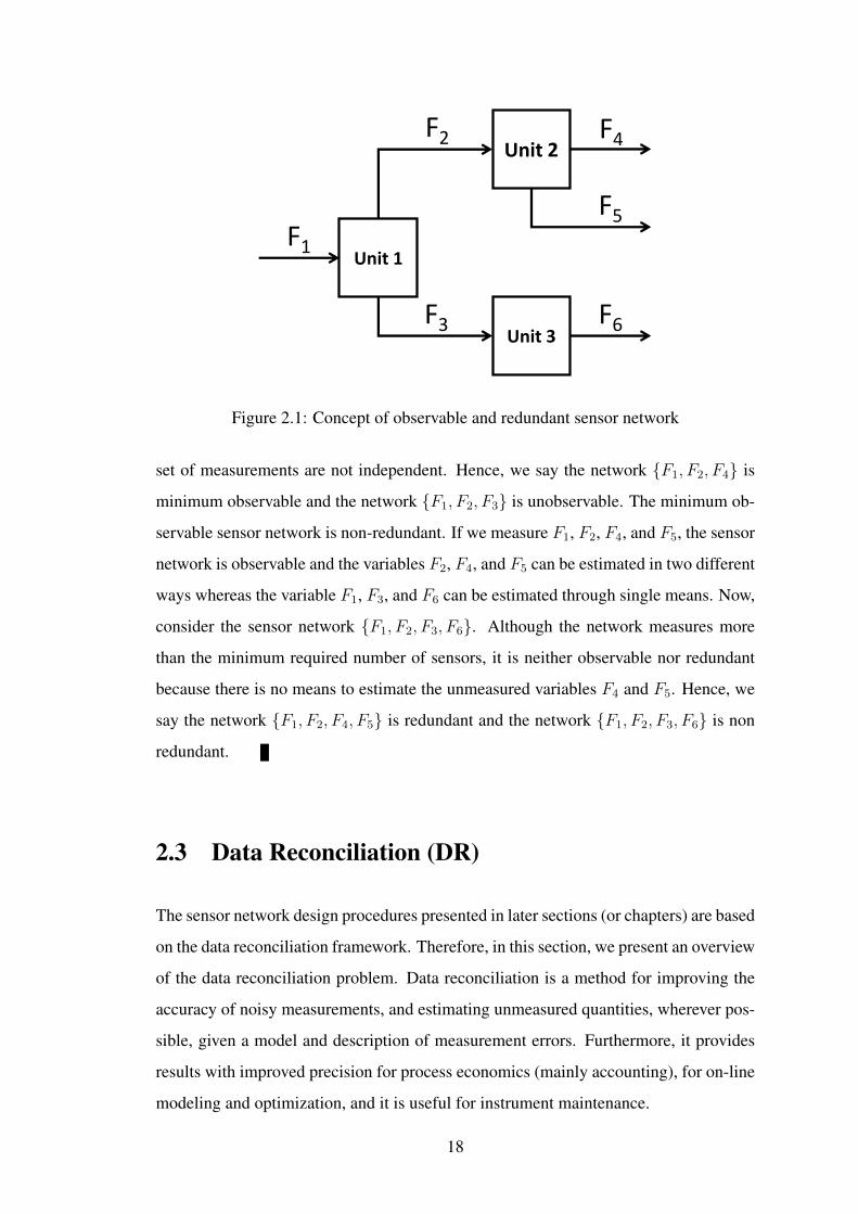
EXAMPLE 2.1

The purpose of this example is to illustrate some of the qualitative properties of sensor

networks. Consider the system with three process units and six streams as depicted in

Figure 2.1. The minimum number of independent sensors required for the system to be

observable under normal operating conditions is three. If F1, F2 and F4 are measured,

then all other variables can be estimated using the model. On the other hand, if we

choose to measure F1, F2, and F3 then we cannot estimate F5 and F6 as the selected

17

Unit 2

Unit 3

Unit 1F1

F2

F3

F4

F5

F6

Figure 2.1: Concept of observable and redundant sensor network

set of measurements are not independent. Hence, we say the network {F1, F2, F4} is

minimum observable and the network {F1, F2, F3} is unobservable. The minimum ob-

servable sensor network is non-redundant. If we measure F1, F2, F4, and F5, the sensor

network is observable and the variables F2, F4, and F5 can be estimated in two different

ways whereas the variable F1, F3, and F6 can be estimated through single means. Now,

consider the sensor network {F1, F2, F3, F6}. Although the network measures more

than the minimum required number of sensors, it is neither observable nor redundant

because there is no means to estimate the unmeasured variables F4 and F5. Hence, we

say the network {F1, F2, F4, F5} is redundant and the network {F1, F2, F3, F6} is non

redundant.

2.3 Data Reconciliation (DR)

The sensor network design procedures presented in later sections (or chapters) are based

on the data reconciliation framework. Therefore, in this section, we present an overview

of the data reconciliation problem. Data reconciliation is a method for improving the

accuracy of noisy measurements, and estimating unmeasured quantities, wherever pos-

sible, given a model and description of measurement errors. Furthermore, it provides

results with improved precision for process economics (mainly accounting), for on-line

modeling and optimization, and it is useful for instrument maintenance.

18

2.3.1 Formulation 1 (Constrained DR problem)

Typically, the linear data reconciliation problem is formulated as follows (Narasimhan

and Jordache, 2000): Consider a vector of measurements denoted by ym of dimension

ny, where ny denotes the number of measurements. This measurement vector is related

to the actual value of the process variable vector, zm, through the measurement equation:

ym = zm + vm (2.1)

where the error vector, vm, is assumed to be normally distributed with zero mean and

diagonal covariance matrix, Σv = E[vmvTm]. Denoting n as the total number of variables

and arranging the remaining (n − ny) unmeasured process variables in vector zu, we

can partition the steady state linearized model (in deviation form) as

A1zm + A2zu = 0 (2.2)

where the number of rows of A1 ( and A2) equals the number of model equations (ne)

representing the process, whereas the number of columns of A1 and A2 equal the num-

ber of measured (ny) and unmeasured variables (n− ny), respectively.

The steady state reconciliation problem is formulated to minimize the appropriate

least square residual such that the model equations are satisfied. Mathematically, the

problem is stated as:

minzm,zu

(ym − zm)TQ(ym − zm) (2.3)

s.t. A1zm + A2zu = 0 (2.4)

where the weighting matrix Q = Σ−1v = diag{ 1

σi2} and σ2

i is the variance of the mea-

surement i. The optimal solution of the problem, zm and zu, is usually called the recon-

ciled value or estimate.

19

2.3.2 Formulation 2 (Unconstrained DR problem)

An alternate but equivalent formulation has been presented by Chmielewski et al. (2002)

in which the variables are classified as: primary variables (zp) and secondary variables

(zs). Denote all possible measurements of interest in the process by z. Then the pri-

mary variables, zp, can be chosen as any subset of process variables (z) that form a

minimum observable set. In other words, primary variables are any set of independent

variables that form a minimum observable set, which can be either measured or un-

measured whereas the remaining variables form a secondary set (see Example 2.2 for

selecting primary and secondary variables). Using this classification of variables, the

process model can be expressed as:

Apzp + Aszs = 0 (2.5)

As the primary variables are selected such that they form a minimum observable net-

work, the matrix As is invertible. Applying block elimination, we have:

zs −Bzp = 0 (2.6)

where B = −A−1s Ap. Now, the set of all variables of interest, z = [zTp z

Ts ] is given by

z = Czp (2.7)

where the matrix C = [I;B] and I is the identity matrix of size equal to the primary

variables. The number of rows of C are equal to the total number of variables, while

the number of columns equal the number of primary variables.

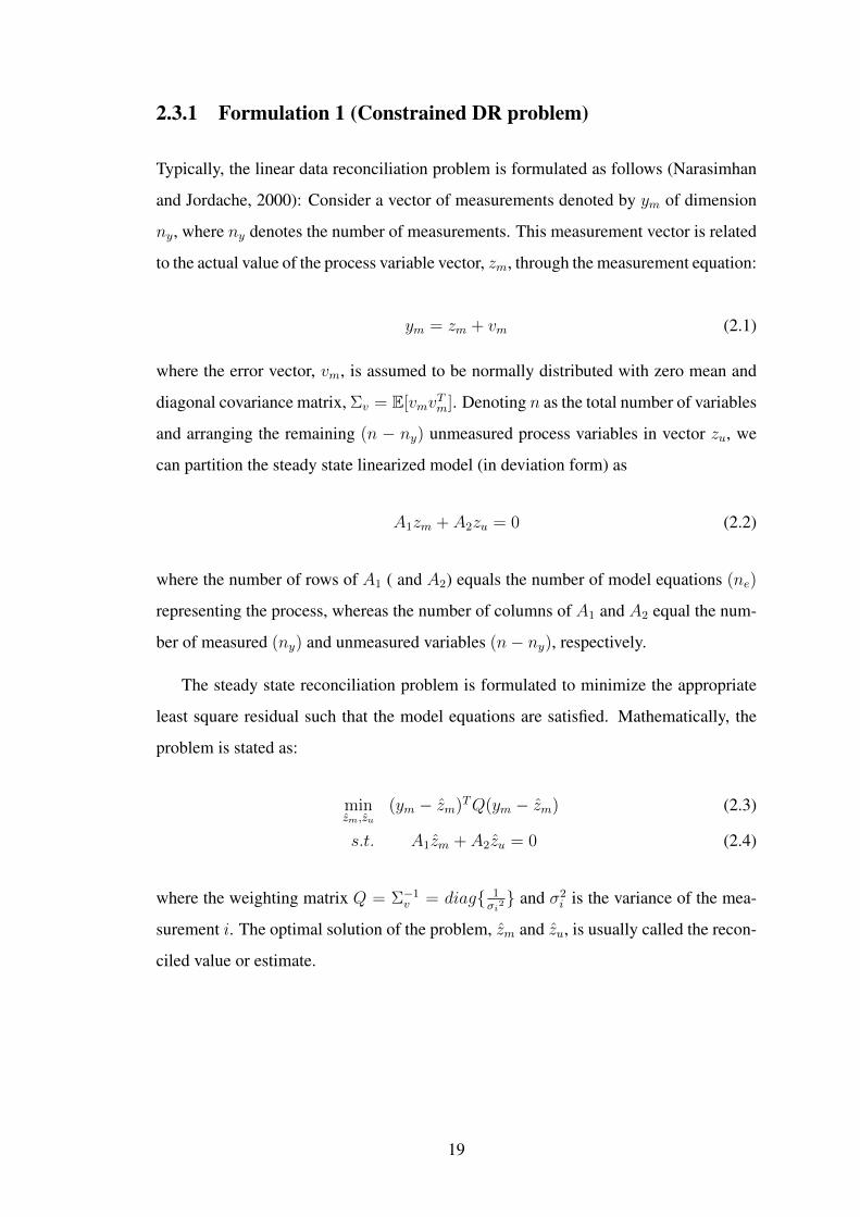
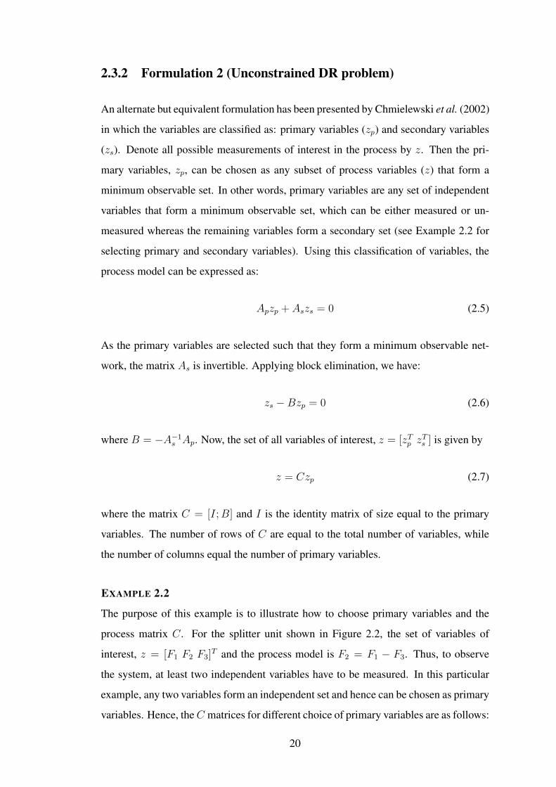
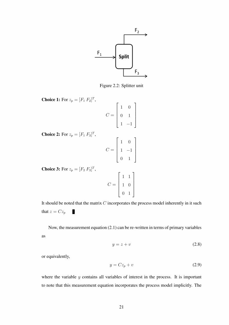
EXAMPLE 2.2

The purpose of this example is to illustrate how to choose primary variables and the

process matrix C. For the splitter unit shown in Figure 2.2, the set of variables of

interest, z = [F1 F2 F3]T and the process model is F2 = F1 − F3. Thus, to observe

the system, at least two independent variables have to be measured. In this particular

example, any two variables form an independent set and hence can be chosen as primary

variables. Hence, theC matrices for different choice of primary variables are as follows:

20

SplitF1

F2

F3

Fig.1 Splitter unitFigure 2.2: Splitter unit

Choice 1: For zp = [F1 F2]T ,

C =

1 0

0 1

1 −1

Choice 2: For zp = [F1 F3]T ,

C =

1 0

1 −1

0 1

Choice 3: For zp = [F2 F3]T ,

C =

1 1

1 0

0 1

It should be noted that the matrix C incorporates the process model inherently in it such

that z = Czp

Now, the measurement equation (2.1) can be re-written in terms of primary variables

as

y = z + v (2.8)

or equivalently,

y = Czp + v (2.9)

where the variable y contains all variables of interest in the process. It is important

to note that this measurement equation incorporates the process model implicitly. The

21

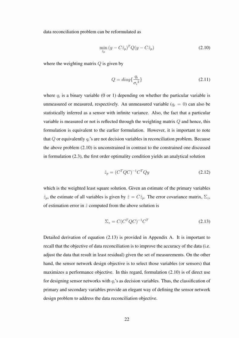
data reconciliation problem can be reformulated as

minzp

(y − Czp)TQ(y − Czp) (2.10)

where the weighting matrix Q is given by

Q = diag{ qiσi2} (2.11)

where qi is a binary variable (0 or 1) depending on whether the particular variable is

unmeasured or measured, respectively. An unmeasured variable (qi = 0) can also be

statistically inferred as a sensor with infinite variance. Also, the fact that a particular

variable is measured or not is reflected through the weighting matrix Q and hence, this

formulation is equivalent to the earlier formulation. However, it is important to note

that Q or equivalently qi’s are not decision variables in reconciliation problem. Because

the above problem (2.10) is unconstrained in contrast to the constrained one discussed

in formulation (2.3), the first order optimality condition yields an analytical solution

zp = (CTQC)−1CTQy (2.12)

which is the weighted least square solution. Given an estimate of the primary variables

zp, the estimate of all variables is given by z = Czp. The error covariance matrix, Σz,

of estimation error in z computed from the above solution is

Σz = C(CTQC)−1CT (2.13)

Detailed derivation of equation (2.13) is provided in Appendix A. It is important to

recall that the objective of data reconciliation is to improve the accuracy of the data (i.e.

adjust the data that result in least residual) given the set of measurements. On the other

hand, the sensor network design objective is to select those variables (or sensors) that

maximizes a performance objective. In this regard, formulation (2.10) is of direct use

for designing sensor networks with qi’s as decision variables. Thus, the classification of

primary and secondary variables provide an elegant way of defining the sensor network

design problem to address the data reconciliation objective.

22

2.4 Sensor Network Design (SND)

The fundamental problem in optimal sensor network design is to choose a set of impor-

tant or strategic process variables to be measured. The selection of measured variables

is an indispensable task for effective control, monitoring, and safe operation of a chem-

ical process. Of the several hundred variables that exist in a typical chemical process,

only a subset of these variables can be measured, because of the nature of the process

and the high cost of measuring instruments. From a computational viewpoint, it is a

combinatorially difficult problem owing to the large number of variables in the process.

For the purpose of efficient process monitoring, a sensor network should be capable of

providing precise information about the state of the process in the presence of random

and gross errors. Kretsovalis and Mah (1987) adopted estimation accuracy as a measure

to choose sensor networks. As an overall measure of estimation accuracy, the sum of

squares of estimation error of all variables (which measures the overall inaccuracy) has

been used. Other measures such as minimizing the log volume of the covariance of the

estimation error (or mean radius) or worst case error variance over all the direction can

also be used (Joshi and Boyd, 2009).

2.4.1 Formulation 3 (SND based on overall error)

The typical objective of a sensor network design problem based on reconciliation frame-

work is to choose the set of measurements so as to minimize the overall estimation error

of the reconciled estimates i.e., Tr(Σz) (Narasimhan and Jordache, 2000) where Tr(.)

denotes the trace operator. Recalling Q = diag{ qiσi2} where qi’s are binary variables.

Notice that qi = 1 implies the variable zi is measured and vice-versa. The sensor net-

work design problem can be mathematically stated using expression (2.13) as:

minqi

Tr(C(CTQC)−1CT ) (2.14)

where the invertibility of CTQC signifies that the system is observable. However for

the overall error to be minimum, CTQC has to be positive definite. Thus, the cur-

rent formulation inherently considers the observability issue and yields an observable

23

sensor network. It should be noted that the formulation (2.14) is a non-linear integer

programming problem.

2.4.2 SDP reformulation

The objective of this subsection is to present the sequence of steps so that the resulting

problem is a semidefinite programming problem with relaxed integer constraints, which

can be solved to global optimality using existing branch and bound solvers. First, we

present here some of the results from convex optimization theory for the sake of conve-

nience,

Fact 01 The epigraph of a function f(x) : Rn → R is defined as epi f = {(x, t)|x ∈

dom f, f(x) ≤ t}. A function is convex if and only if its epigraph is a convex

set.

Fact 02 If D is positive definite, i.e., D � 0, then the matrix S = A − BD−1BT is

called the Schur complement of D in the matrix X =

A B

BT D

. Then the

condition for positive semi-definiteness of block matrix X is: If D � 0, then

X � 0 if and only if S � 0

Using the definition of epigraph of the function (see Fact 01), the non-linear integer

programming formulation (2.14) can be rewritten using a scalar cost function (te) as

minte,qi

Lerror = te (2.15a)

s.t. T r(C(CTQC)−1CT ) ≤ te (2.15b)

Now, introducing a positive definite (or semidefinite) matrix (Ye), the last inequality

constraint (2.15b) can be written as

Tr(Ye) ≤ te (2.16a)

Ye − C(CTQC)−1CT � 0 (2.16b)

24

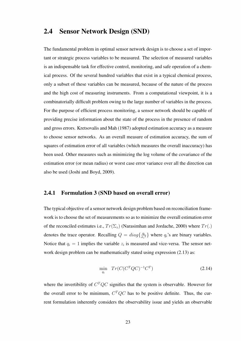
Using Schur complement (see Fact 02), the matrix inequality constraint (2.16b) can be

written in LMI form,

Ye C

CT (CTQC)

� 0; (2.17)

The sub matrix, (CTQC), in the above LMI has to be positive definite for the LMI

to be positive definite. Hence the observability of the sensor network is ensured if the

LMI is satisfied. Therefore, the sensor network design problem that finds k sensors that

minimizes the overall estimation error is cast as

minqi,te,Ye

Lerror = te (2.18a)

s.t. T r(Ye) ≤ te (2.18b) Ye C

CT (CTQC)

� 0 (2.18c)

qi ∈ {0, 1} (2.18d)

Q = diag{ qiσi2} (2.18e)∑nz

i=1 qi = k (2.18f)

Additionally, we imposed a cardinality constraint (2.18f) to limit the number of sensors

being selected. For the system to be observable, we need to choose a value of k greater

than or equal to the minimum number of sensors. The minimum number of sensors

required for the system to be observable is given by the steady state degrees of freedom

of the system, which is defined as the number of variables minus number of equations.

The integer restriction of qi ∈ {0, 1} makes the above formulation non-convex. How-

ever, linear relaxation of qi (i.e., 0 ≤ qi ≤ 1) results in a convex SDP problem. Hence,

we can solve the problem to determine globally optimal sensor network using available

solvers (Löfberg, 2004). A branch and bound algorithm which uses the internal SDPT3

solver (to solve the SDP with linear relaxation at each branching step) is used to solve

the problem.

25

Example: Simple Ammonia Network

F2 - F1 - F7 = 0

F3 - F2 = 0

F4 - F3 = 0

F5 + F6 - F4 = 0

F7 + F8 - F5 = 0MIX HEX

SPL

REA SEP

F1 F2 F3 F4

F5

F6

F8

F7

Fig. 5 Simple Ammonia NetworkFigure 2.3: Simple ammonia process

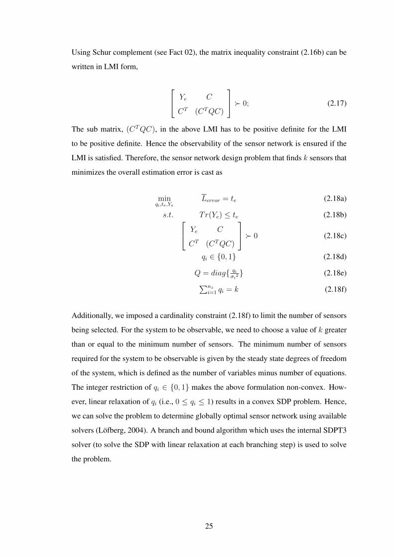
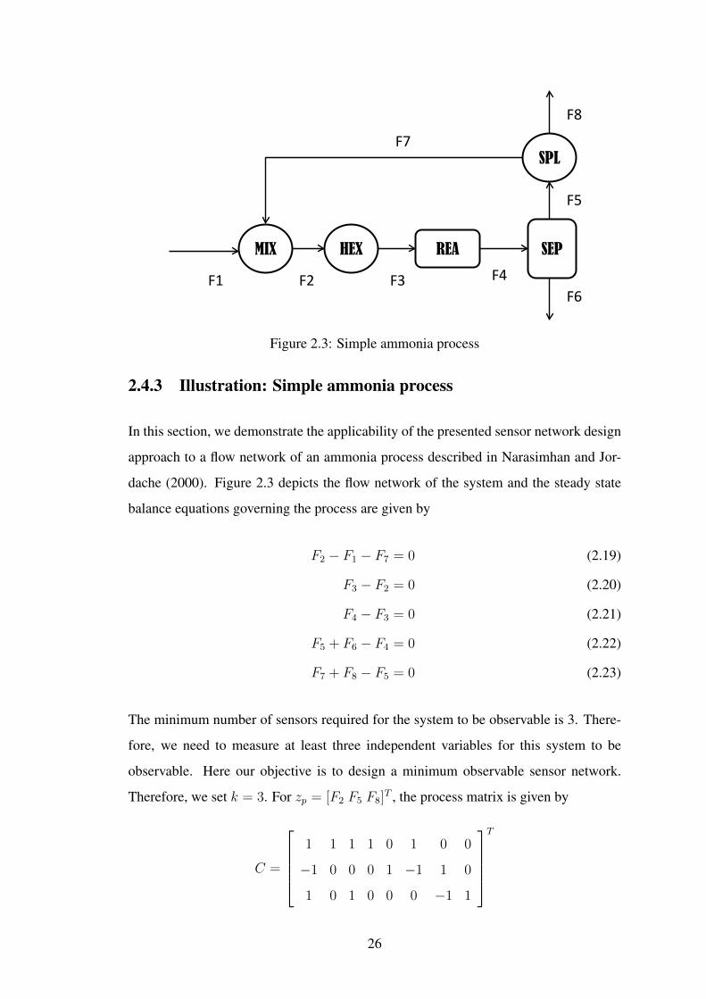
2.4.3 Illustration: Simple ammonia process

In this section, we demonstrate the applicability of the presented sensor network design

approach to a flow network of an ammonia process described in Narasimhan and Jor-

dache (2000). Figure 2.3 depicts the flow network of the system and the steady state

balance equations governing the process are given by

F2 − F1 − F7 = 0 (2.19)

F3 − F2 = 0 (2.20)

F4 − F3 = 0 (2.21)

F5 + F6 − F4 = 0 (2.22)

F7 + F8 − F5 = 0 (2.23)

The minimum number of sensors required for the system to be observable is 3. There-

fore, we need to measure at least three independent variables for this system to be

observable. Here our objective is to design a minimum observable sensor network.

Therefore, we set k = 3. For zp = [F2 F5 F8]T , the process matrix is given by

C =

1 1 1 1 0 1 0 0

−1 0 0 0 1 −1 1 0

1 0 1 0 0 0 −1 1

T

26

The formulation (2.18) can be solved to global optimality using YALMIP, a freely avail-

able toolbox for solving convex and non convex optimization problems in MATLAB

(Löfberg, 2004). Assuming the variance of the measured variable to be unity, the sen-

sor network which has a minimal overall error was found to be {F3, F5, F7} and the

overall error value is 11.

2.5 Summary

In this chapter, we presented an overview of data reconciliation problem to obtain better

estimates of process variables. Since the choice of measured variables is critical for rec-

onciliation activity, the sensor network design procedure that uses mean squared error

as a measure of estimation accuracy was discussed. Next, an MICP reformulation of the

sensor network design problem was set-up which is solved to global optimality using

available solvers. However, such a sensor network design procedure cannot guarantee

the economic benefit one would achieve by selecting measurements. This will be dealt

in the next chapter.

27

CHAPTER 3

SENSOR NETWORK DESIGN FOR OPTIMAL

PROCESS OPERATIONS

Based on the paper published in Industrial & Engineering Chemistry Research

The focus of this chapter is to develop a sensor network design procedure that re-

lates process economics and precision of estimates obtained by data reconciliation. For

this purpose, we define an average loss function, which could incorporate the loss in

operational profit due to model uncertainties, disturbances and measurement errors.

However, the current study focuses on the loss incurred due to measurements corrupted

by random Gaussian errors only. The resulting analytical expression that quantifies the

loss is shown to be the sum of weighted error variances of the reconciled estimates

obtained from reconciliation. Similar to the SDP based sensor network design proce-

dure presented in Chapter 2, we present the formulation that minimizes the average loss

function. Demonstrative examples are provided to illustrate the approach.

As discussed in Chapter 1, the optimal operation of a chemical process depends

on various structural and parametric decisions. Selection of sensors is an important

structural decision for the safe and optimal operation of a chemical plant. The sensor

selection procedures for the purpose of data reconciliation typically uses some measure

of estimation accuracy such as mean squared error, mean radius or worst case error vari-

ance over all direction. However, the resulting sensor network using such performance

measures need not select the economically important variables as measurements. This

is illustrated using the following Example 3.1.

EXAMPLE 3.1

This example illustrates the need for a new profit based metric to quantify the sensor

network. Consider the process unit presented in Example 2.2. Assuming the variance

of the measured variable to be unity, the error covariance matrices for different sensor

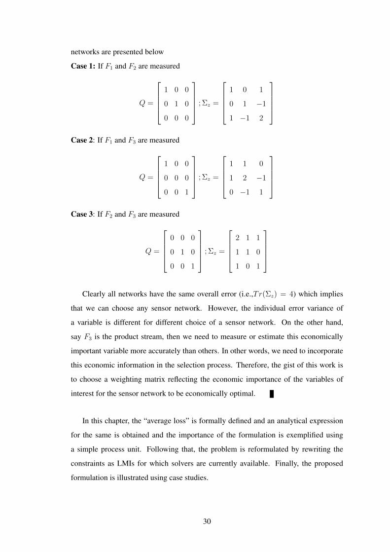
networks are presented below

Case 1: If F1 and F2 are measured

Q =

1 0 0

0 1 0

0 0 0

; Σz =

1 0 1

0 1 −1

1 −1 2

Case 2: If F1 and F3 are measured

Q =

1 0 0

0 0 0

0 0 1

; Σz =

1 1 0

1 2 −1

0 −1 1

Case 3: If F2 and F3 are measured

Q =

0 0 0

0 1 0

0 0 1

; Σz =

2 1 1

1 1 0

1 0 1

Clearly all networks have the same overall error (i.e.,Tr(Σz) = 4) which implies

that we can choose any sensor network. However, the individual error variance of

a variable is different for different choice of a sensor network. On the other hand,

say F3 is the product stream, then we need to measure or estimate this economically

important variable more accurately than others. In other words, we need to incorporate

this economic information in the selection process. Therefore, the gist of this work is

to choose a weighting matrix reflecting the economic importance of the variables of

interest for the sensor network to be economically optimal.

In this chapter, the “average loss” is formally defined and an analytical expression

for the same is obtained and the importance of the formulation is exemplified using

a simple process unit. Following that, the problem is reformulated by rewriting the

constraints as LMIs for which solvers are currently available. Finally, the proposed

formulation is illustrated using case studies.

30

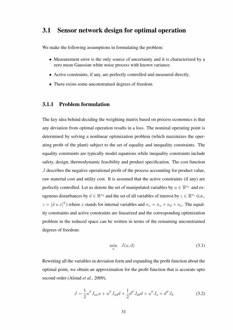
3.1 Sensor network design for optimal operation

We make the following assumptions in formulating the problem:

• Measurement error is the only source of uncertainty and it is characterized by azero mean Gaussian white noise process with known variance.

• Active constraints, if any, are perfectly controlled and measured directly.

• There exists some unconstrained degrees of freedom.

3.1.1 Problem formulation

The key idea behind deciding the weighting matrix based on process economics is that

any deviation from optimal operation results in a loss. The nominal operating point is

determined by solving a nonlinear optimization problem (which maximizes the oper-

ating profit of the plant) subject to the set of equality and inequality constraints. The

equality constraints are typically model equations while inequality constraints include

safety, design, thermodynamic feasibility and product specification. The cost function

J describes the negative operational profit of the process accounting for product value,

raw material cost and utility cost. It is assumed that the active constraints (if any) are

perfectly controlled. Let us denote the set of manipulated variables by u ∈ Rnu and ex-

ogenous disturbances by d ∈ Rnd and the set of all variables of interest by z ∈ Rnz (i.e.,

z = [d u x]T ) where x stands for internal variables and nz = nu + nd + nx. The equal-

ity constraints and active constraints are linearized and the corresponding optimization

problem in the reduced space can be written in terms of the remaining unconstrained

degrees of freedom:

minu

J(u, d) (3.1)

Rewriting all the variables in deviation form and expanding the profit function about the

optimal point, we obtain an approximation for the profit function that is accurate upto

second order (Alstad et al., 2009),

J =1

2uTJuuu+ uTJudd+

1

2dTJddd+ uTJu + dTJd (3.2)

31

Assuming the nominal point is optimal, Ju = 0. From the first order optimality condi-

tion, the optimal values of u and the associated cost function is found to be

u∗ = −J−1uu Judd (3.3)

J∗ = −1

2dTJTud(J

−1uu )TJudd+

1

2dTJddd+ dTJd (3.4)

However, in reality, equation (3.3) cannot be satisfied exactly due to uncertainty in

the model and measurements. Here, we assume that the only source of uncertainty is

random errors affecting the measurements. When all variables z are observable, the

reconciled estimates, u and d will satisfy the following:

u = −J−1uu Judd (3.5)

In this work, we assume that a suitable controller is available for implementing the

optimal strategy and to control active constraints. Now, we can equivalently express the

above equation as

u∗ + εu = −J−1uu Jud(d+ εd) (3.6)

where εd and εu are the errors in the estimate of d and u∗ respectively. The resulting

achieved cost, J can be expressed as follows:

J = −1

2dTJTud(J

−1uu )TJudd+

1

2dTJTud(J

−1uu )TJudεd +

1

2dTJTud(J

−1uu )TJuuεu

−1

2εTd J

Tud(J

−1uu )TJudd+

1

2εTd J

Tud(J

−1uu )TJudεd +

1

2εTd J

Tud(J

−1uu )TJuuεu

−1

2εTuJudd+

1

2εTuJudεd +

1

2εTuJuuεu +

1

2dTJddd+ dTJd (3.7)

where J ≥ J∗ and hence any implementation strategy results in a loss. Due to the

randomness in measurement error, we express the term average loss as the statistical

expectation of the deviation of the achieved cost from the optimal cost. Mathematically,

the average loss, Lcost is defined as

Lcost = E(J − J∗) (3.8)

32

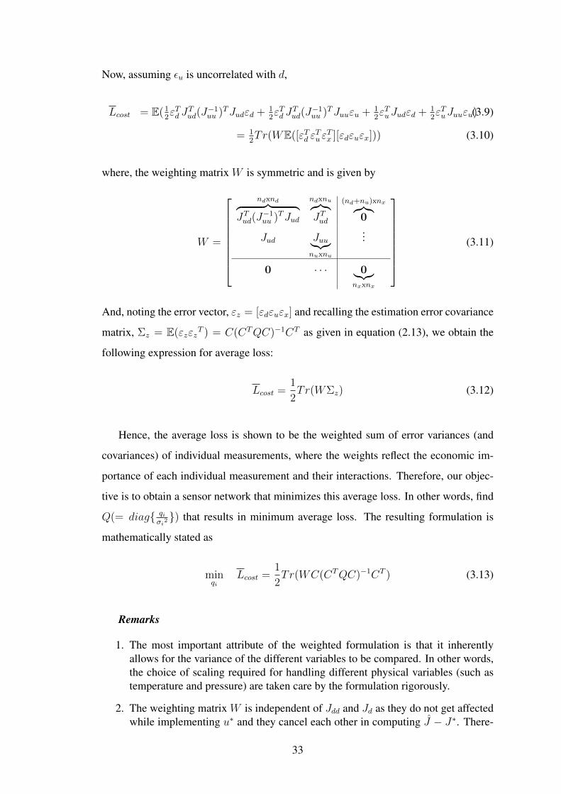
Now, assuming εu is uncorrelated with d,

Lcost = E(12εTd J

Tud(J

−1uu )TJudεd + 1

2εTd J

Tud(J

−1uu )TJuuεu + 1

2εTuJudεd + 1

2εTuJuuεu)(3.9)

= 12Tr(WE([εTd ε

Tu ε

Tx ][εdεuεx])) (3.10)

where, the weighting matrix W is symmetric and is given by

W =

ndxnd︷ ︸︸ ︷JTud(J

−1uu )TJud

ndxnu︷︸︸︷JTud

(nd+nu)xnx︷︸︸︷0

Jud Juu︸︷︷︸nuxnu

...

0 · · · 0︸︷︷︸nxxnx

(3.11)

And, noting the error vector, εz = [εdεuεx] and recalling the estimation error covariance

matrix, Σz = E(εzεzT ) = C(CTQC)−1CT as given in equation (2.13), we obtain the

following expression for average loss:

Lcost =1

2Tr(WΣz) (3.12)

Hence, the average loss is shown to be the weighted sum of error variances (and

covariances) of individual measurements, where the weights reflect the economic im-

portance of each individual measurement and their interactions. Therefore, our objec-

tive is to obtain a sensor network that minimizes this average loss. In other words, find

Q(= diag{ qiσi2}) that results in minimum average loss. The resulting formulation is

mathematically stated as

minqi

Lcost =1

2Tr(WC(CTQC)−1CT ) (3.13)

Remarks

1. The most important attribute of the weighted formulation is that it inherentlyallows for the variance of the different variables to be compared. In other words,the choice of scaling required for handling different physical variables (such astemperature and pressure) are taken care by the formulation rigorously.

2. The weighting matrix W is independent of Jdd and Jd as they do not get affectedwhile implementing u∗ and they cancel each other in computing J − J∗. There-

33

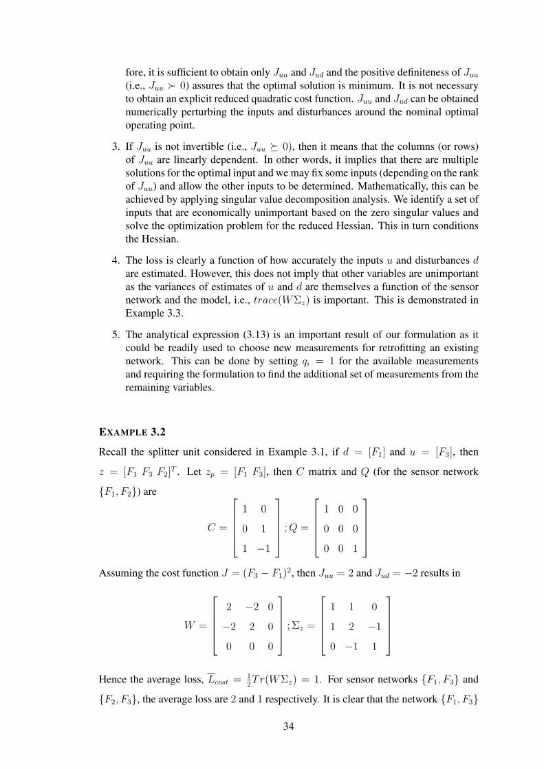
fore, it is sufficient to obtain only Juu and Jud and the positive definiteness of Juu(i.e., Juu � 0) assures that the optimal solution is minimum. It is not necessaryto obtain an explicit reduced quadratic cost function. Juu and Jud can be obtainednumerically perturbing the inputs and disturbances around the nominal optimaloperating point.

3. If Juu is not invertible (i.e., Juu � 0), then it means that the columns (or rows)of Juu are linearly dependent. In other words, it implies that there are multiplesolutions for the optimal input and we may fix some inputs (depending on the rankof Juu) and allow the other inputs to be determined. Mathematically, this can beachieved by applying singular value decomposition analysis. We identify a set ofinputs that are economically unimportant based on the zero singular values andsolve the optimization problem for the reduced Hessian. This in turn conditionsthe Hessian.

4. The loss is clearly a function of how accurately the inputs u and disturbances dare estimated. However, this does not imply that other variables are unimportantas the variances of estimates of u and d are themselves a function of the sensornetwork and the model, i.e., trace(WΣz) is important. This is demonstrated inExample 3.3.

5. The analytical expression (3.13) is an important result of our formulation as itcould be readily used to choose new measurements for retrofitting an existingnetwork. This can be done by setting qi = 1 for the available measurementsand requiring the formulation to find the additional set of measurements from theremaining variables.

EXAMPLE 3.2

Recall the splitter unit considered in Example 3.1, if d = [F1] and u = [F3], then

z = [F1 F3 F2]T . Let zp = [F1 F3], then C matrix and Q (for the sensor network

{F1, F2}) are

C =

1 0

0 1

1 −1

;Q =

1 0 0

0 0 0

0 0 1

Assuming the cost function J = (F3 − F1)2, then Juu = 2 and Jud = −2 results in

W =

2 −2 0

−2 2 0

0 0 0

; Σz =

1 1 0

1 2 −1

0 −1 1

Hence the average loss, Lcost = 1

2Tr(WΣz) = 1. For sensor networks {F1, F3} and

{F2, F3}, the average loss are 2 and 1 respectively. It is clear that the network {F1, F3}

34

is not economically optimal. This simple unit is presented to illustrate the basic idea.

EXAMPLE 3.3

Recall the splitter unit considered in Example 3.2, if d = [F1] and u = [F3], then

z = [F1 F3 F2]T . Let zp = [F1 F3], then C matrix and Q (assuming unit variance for all

flow variables) are

C =

1 0

0 1

1 −1

;Q =

q1 0 0

0 q2 0

0 0 q3

The error covariance matrix, Σz, can be expressed in terms of sensor network using

(2.13) as

Σz =1

q1q2 + q1q3 + q2q3

q2 + q3 q3 q2

q3 q1 + q3 −q1

q2 −q1 q1 + q2

Let us consider the weighting matrix of the form

W =

w11 w12 0

w21 w22 0

0 0 0

Now the sensor network design formulation (3.13) based on average loss function, after

simplification, is given by

Lcost =w11(q2 + q3) + (w12 + w21)q3 + w22(q1 + q3)

2(q1q2 + q1q3 + q2q3)

Clearly the average loss function, Lcost, is a function of covariance estimates of all the

process variables, which are, indeed, functions of sensor network we choose among all

process variables of interest. It is important to note that the covariance estimates are not

just the functions of manipulated (F3) and disturbance variables (F1) only.

35

3.1.2 Mixed Integer Cone Program (MICP)

The weighted formulation (3.13) is a non-linear integer programming problem. How-

ever, we can pose the problem with integer relaxations as a semidefinite programming

problem similar to the one discussed in Section 2.4.2. The resulting MICP can be solved

using available software to obtain globally optimal solutions.

First, we factorize the weighting matrix as W = RRT , where R is a positive semi-

definite square root of W to induce symmetry in the matrix inequality. Invoking the

property that trace operator is invariant under cyclic permutations (i.e., Tr(ABD) =

Tr(BDA) = Tr(DAB) 6= Tr(ADB)), the average loss can be expressed as (Refer

equation 3.13)

L =1

2Tr(WC(CTQC)−1CT ) (3.14)

=1

2Tr(RRTC(CTQC)−1CT ) (3.15)

=1

2Tr(RTC(CTQC)−1CTR) (3.16)

In the overall error formulation, we selected ’k’ sensors such that k is any value

greater than Nmin where Nmin is the number of degrees of freedom of the system con-

sidered required for observability. Thus the sum of all qi is set to k,

nz∑i=1

qi = k (3.17)

The above constraint allows one to find a redundant sensor network if you set k >

Nmin . It is well known that redundancy in measurements improves the quality of the

reconciled estimates. Thus, selecting more measurements improves the accuracy of the

estimates which in turn reduces the average loss as a result of error reduction. However

this might lead to a situation where all measurements are selected if you set k ≥ Nmin.

On the other hand, it is more meaningful to impose a constraint on the available capital

cost. Thus, the capital cost constraints to account for the available resource limit (c∗)

36

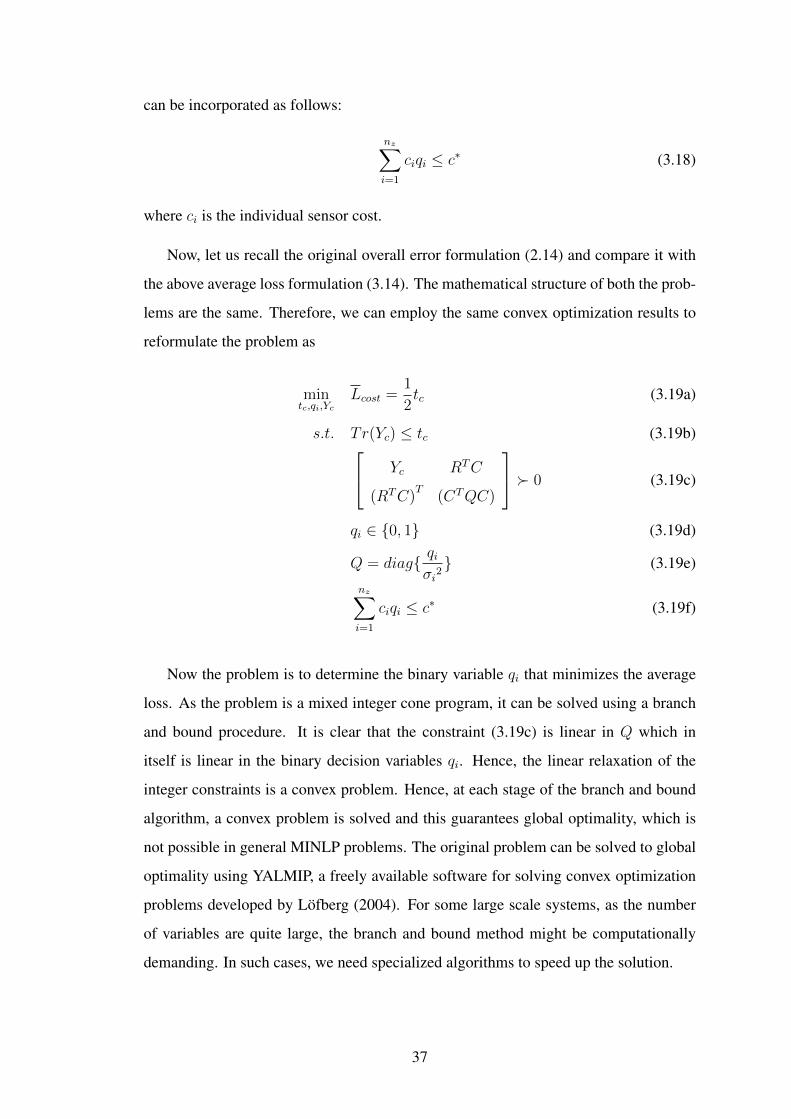
can be incorporated as follows:

nz∑i=1

ciqi ≤ c∗ (3.18)

where ci is the individual sensor cost.

Now, let us recall the original overall error formulation (2.14) and compare it with

the above average loss formulation (3.14). The mathematical structure of both the prob-

lems are the same. Therefore, we can employ the same convex optimization results to

reformulate the problem as

mintc,qi,Yc

Lcost =1

2tc (3.19a)

s.t. T r(Yc) ≤ tc (3.19b) Yc RTC

(RTC)T

(CTQC)

� 0 (3.19c)

qi ∈ {0, 1} (3.19d)

Q = diag{ qiσi2} (3.19e)

nz∑i=1

ciqi ≤ c∗ (3.19f)

Now the problem is to determine the binary variable qi that minimizes the average

loss. As the problem is a mixed integer cone program, it can be solved using a branch

and bound procedure. It is clear that the constraint (3.19c) is linear in Q which in

itself is linear in the binary decision variables qi. Hence, the linear relaxation of the

integer constraints is a convex problem. Hence, at each stage of the branch and bound

algorithm, a convex problem is solved and this guarantees global optimality, which is

not possible in general MINLP problems. The original problem can be solved to global

optimality using YALMIP, a freely available software for solving convex optimization

problems developed by Löfberg (2004). For some large scale systems, as the number

of variables are quite large, the branch and bound method might be computationally

demanding. In such cases, we need specialized algorithms to speed up the solution.

37

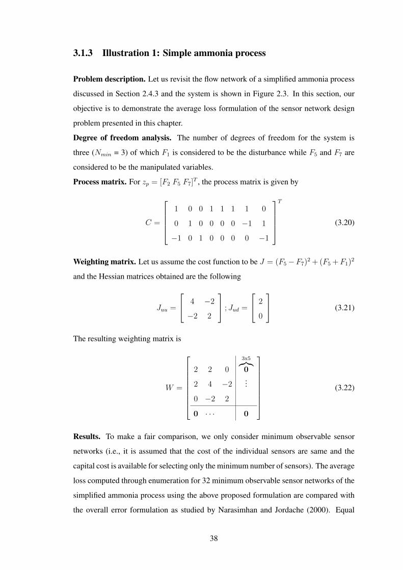
3.1.3 Illustration 1: Simple ammonia process

Problem description. Let us revisit the flow network of a simplified ammonia process

discussed in Section 2.4.3 and the system is shown in Figure 2.3. In this section, our

objective is to demonstrate the average loss formulation of the sensor network design

problem presented in this chapter.

Degree of freedom analysis. The number of degrees of freedom for the system is

three (Nmin = 3) of which F1 is considered to be the disturbance while F5 and F7 are

considered to be the manipulated variables.

Process matrix. For zp = [F2 F5 F7]T , the process matrix is given by

C =

1 0 0 1 1 1 1 0

0 1 0 0 0 0 −1 1

−1 0 1 0 0 0 0 −1

T

(3.20)

Weighting matrix. Let us assume the cost function to be J = (F5−F7)2 + (F5 +F1)2

and the Hessian matrices obtained are the following

Juu =

4 −2

−2 2

; Jud =

2

0

(3.21)

The resulting weighting matrix is

W =

2 2 0

3x5︷︸︸︷0

2 4 −2...

0 −2 2

0 · · · 0

(3.22)

Results. To make a fair comparison, we only consider minimum observable sensor

networks (i.e., it is assumed that the cost of the individual sensors are same and the

capital cost is available for selecting only the minimum number of sensors). The average

loss computed through enumeration for 32 minimum observable sensor networks of the

simplified ammonia process using the above proposed formulation are compared with

the overall error formulation as studied by Narasimhan and Jordache (2000). Equal

38

sensor cost and unit variance are assumed in this example to explain the contribution

of the operating profit, and the results obtained are listed in Table 3.1. For the cost

function considered above, the first term represents the importance of F8 while the

other term signify the combined importance of F1 and F5. Hence it is trivial that the

network {F1, F5, F8} is economically optimal since it is observable. Therefore, to select

other combinations, it is tempting to choose the network that contains F8 as a variable

since it has direct effect. However, because of the propagation of errors in estimating

the other variables (i.e. indirect effect), the average loss could still be higher. For

instance, consider the network {F6, F7, F8} which incur the loss of $ 7/h while the

other network {F1, F5, F6} is better as the loss is $ 4/h. It is important to note that there

are multiple economically optimal solutions. In summary, the optimal sensor network

obtained using our formulation is based on the combined effect of process profit and the

error propagation as explained by weighting and error covariance matrix, respectively.

Table 3.1: Comparison of average loss and overall error of a simple ammonia process

Sensor Average Overall Sensor Average OverallNetwork loss ($/h) Error+ Network loss ($/h) Error+

F1, F2, F5 5 12 F1, F2, F6 5 11F1, F2, F8 3 12 F2, F5, F7 5 11*F2, F5, F8 3 12 F2, F6, F7 9 12F2, F6, F8 3 12 F2, F7, F8 3 12F1, F3, F5 5 12 F1, F3, F6 5 11F1, F3, F8 3 12 F3, F5, F7 5 11F3, F5, F8 3 12 F3, F6, F7 9 12F3, F6, F8 3 12 F3, F7, F8 3 12F1, F4, F5 5 12 F1, F4, F6 5 11F1, F4, F8 3 12 F4, F5, F7 5 11F4, F5, F8 3 12 F4, F6, F7 9 12F4, F6, F8 3 12 F4, F7, F8 3 12F1, F5, F6 4 14 F1, F5, F7 4 14F1, F5, F8 3* 16 F1, F6, F7 8 14F1, F7, F8 4 13 F5, F6, F7 8 14F5, F6, F8 4 13 F6, F7, F8 7 16* indicates YALMIP branch and bound solution obtained using sdpt3 solver+ results from Narasimhan and Jordache (2000)

39

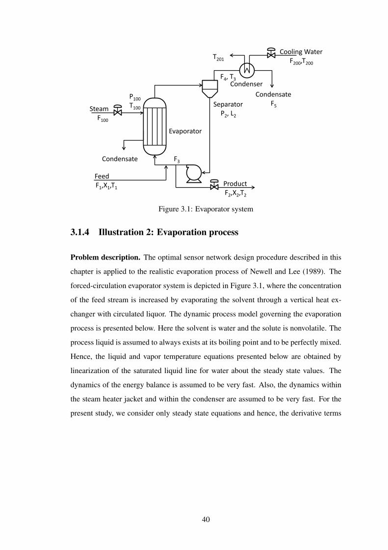
Condensate

CondensateF5

Condenser

SteamF100

FeedF1,X1,T1

F3

ProductF2,X2,T2

SeparatorP2, L2

Cooling WaterF200,T200

T201

F4, T3

P100T100

Evaporator

Figure 3.1: Evaporator system

3.1.4 Illustration 2: Evaporation process

Problem description. The optimal sensor network design procedure described in this

chapter is applied to the realistic evaporation process of Newell and Lee (1989). The

forced-circulation evaporator system is depicted in Figure 3.1, where the concentration

of the feed stream is increased by evaporating the solvent through a vertical heat ex-

changer with circulated liquor. The dynamic process model governing the evaporation

process is presented below. Here the solvent is water and the solute is nonvolatile. The

process liquid is assumed to always exists at its boiling point and to be perfectly mixed.

Hence, the liquid and vapor temperature equations presented below are obtained by

linearization of the saturated liquid line for water about the steady state values. The

dynamics of the energy balance is assumed to be very fast. Also, the dynamics within

the steam heater jacket and within the condenser are assumed to be very fast. For the

present study, we consider only steady state equations and hence, the derivative terms

40

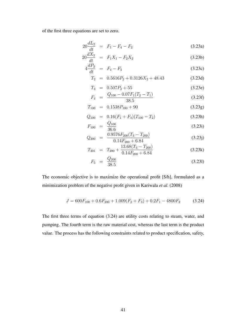
of the first three equations are set to zero.

20dL2

dt= F1 − F4 − F2 (3.23a)

20dX2

dt= F1X1 − F2X2 (3.23b)

4dP2

dt= F4 − F5 (3.23c)

T2 = 0.5616P2 + 0.3126X2 + 48.43 (3.23d)

T3 = 0.507P2 + 55 (3.23e)

F4 =Q100 − 0.07F1(T2 − T1)

38.5(3.23f)

T100 = 0.1538P100 + 90 (3.23g)

Q100 = 0.16(F1 + F3)(T100 − T2) (3.23h)

F100 =Q100

36.6(3.23i)

Q200 =0.9576F200(T3 − T200)

0.14F200 + 6.84(3.23j)

T201 = T200 +13.68(T3 − T200)

0.14F200 + 6.84(3.23k)

F5 =Q200

38.5(3.23l)

The economic objective is to maximize the operational profit [$/h], formulated as a

minimization problem of the negative profit given in Kariwala et al. (2008)

J = 600F100 + 0.6F200 + 1.009(F2 + F3) + 0.2F1 − 4800F2 (3.24)

The first three terms of equation (3.24) are utility costs relating to steam, water, and

pumping. The fourth term is the raw material cost, whereas the last term is the product

value. The process has the following constraints related to product specification, safety,

41

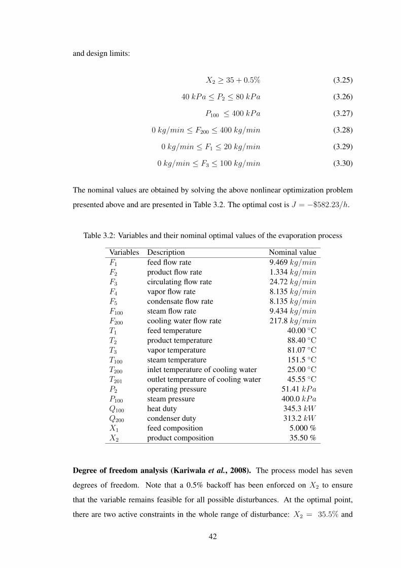
and design limits:

X2 ≥ 35 + 0.5% (3.25)

40 kPa ≤ P2 ≤ 80 kPa (3.26)

P100 ≤ 400 kPa (3.27)

0 kg/min ≤ F200 ≤ 400 kg/min (3.28)

0 kg/min ≤ F1 ≤ 20 kg/min (3.29)

0 kg/min ≤ F3 ≤ 100 kg/min (3.30)

The nominal values are obtained by solving the above nonlinear optimization problem

presented above and are presented in Table 3.2. The optimal cost is J = −$582.23/h.

Table 3.2: Variables and their nominal optimal values of the evaporation process

Variables Description Nominal valueF1 feed flow rate 9.469 kg/minF2 product flow rate 1.334 kg/minF3 circulating flow rate 24.72 kg/minF4 vapor flow rate 8.135 kg/minF5 condensate flow rate 8.135 kg/minF100 steam flow rate 9.434 kg/minF200 cooling water flow rate 217.8 kg/minT1 feed temperature 40.00 ◦CT2 product temperature 88.40 ◦CT3 vapor temperature 81.07 ◦CT100 steam temperature 151.5 ◦CT200 inlet temperature of cooling water 25.00 ◦CT201 outlet temperature of cooling water 45.55 ◦CP2 operating pressure 51.41 kPaP100 steam pressure 400.0 kPaQ100 heat duty 345.3 kWQ200 condenser duty 313.2 kWX1 feed composition 5.000 %X2 product composition 35.50 %

Degree of freedom analysis (Kariwala et al., 2008). The process model has seven

degrees of freedom. Note that a 0.5% backoff has been enforced on X2 to ensure

that the variable remains feasible for all possible disturbances. At the optimal point,

there are two active constraints in the whole range of disturbance: X2 = 35.5% and

42

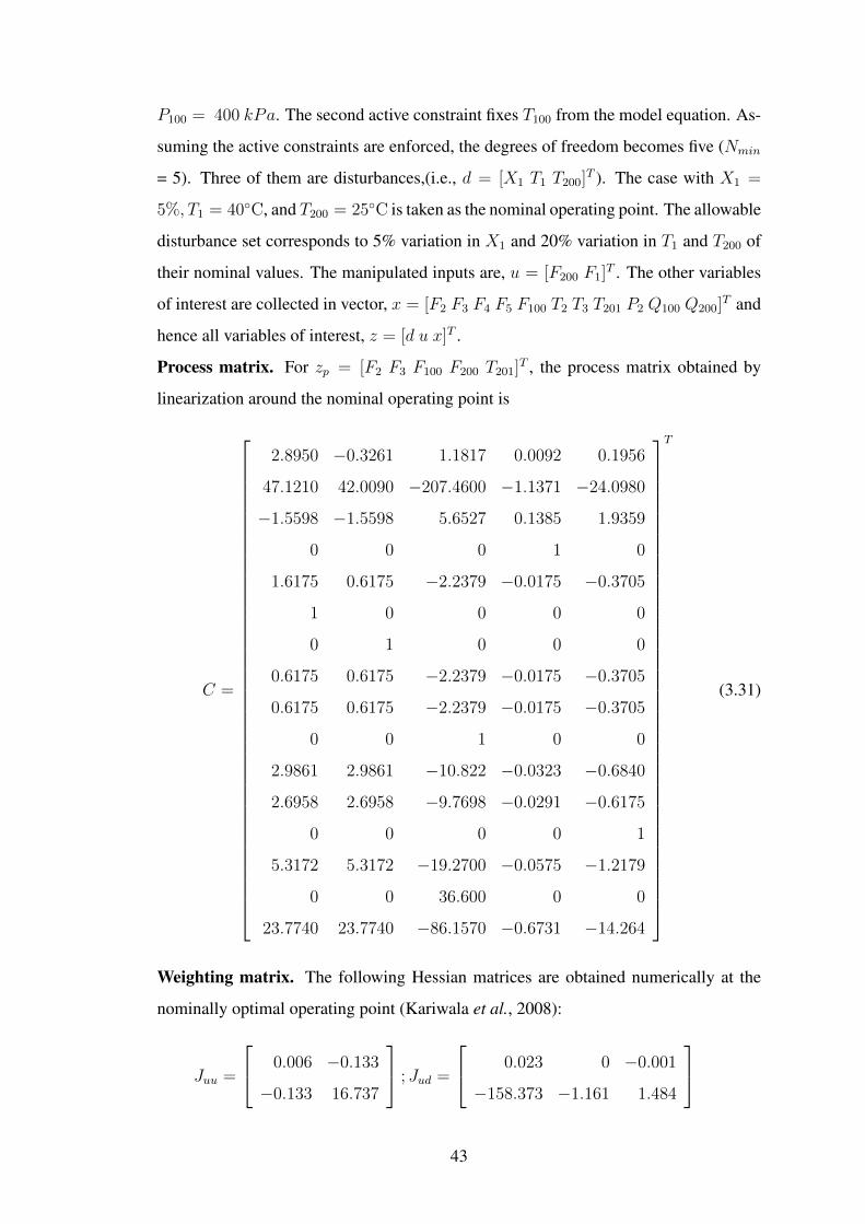
P100 = 400 kPa. The second active constraint fixes T100 from the model equation. As-

suming the active constraints are enforced, the degrees of freedom becomes five (Nmin

= 5). Three of them are disturbances,(i.e., d = [X1 T1 T200]T ). The case with X1 =

5%, T1 = 40◦C, and T200 = 25◦C is taken as the nominal operating point. The allowable

disturbance set corresponds to 5% variation in X1 and 20% variation in T1 and T200 of

their nominal values. The manipulated inputs are, u = [F200 F1]T . The other variables

of interest are collected in vector, x = [F2 F3 F4 F5 F100 T2 T3 T201 P2 Q100 Q200]T and

hence all variables of interest, z = [d u x]T .

Process matrix. For zp = [F2 F3 F100 F200 T201]T , the process matrix obtained by

linearization around the nominal operating point is

C =

2.8950 −0.3261 1.1817 0.0092 0.1956

47.1210 42.0090 −207.4600 −1.1371 −24.0980

−1.5598 −1.5598 5.6527 0.1385 1.9359

0 0 0 1 0

1.6175 0.6175 −2.2379 −0.0175 −0.3705

1 0 0 0 0

0 1 0 0 0

0.6175 0.6175 −2.2379 −0.0175 −0.3705

0.6175 0.6175 −2.2379 −0.0175 −0.3705

0 0 1 0 0

2.9861 2.9861 −10.822 −0.0323 −0.6840

2.6958 2.6958 −9.7698 −0.0291 −0.6175

0 0 0 0 1

5.3172 5.3172 −19.2700 −0.0575 −1.2179

0 0 36.600 0 0

23.7740 23.7740 −86.1570 −0.6731 −14.264

T

(3.31)

Weighting matrix. The following Hessian matrices are obtained numerically at the

nominally optimal operating point (Kariwala et al., 2008):

Juu =

0.006 −0.133

−0.133 16.737

; Jud =

0.023 0 −0.001

−158.373 −1.161 1.484

43

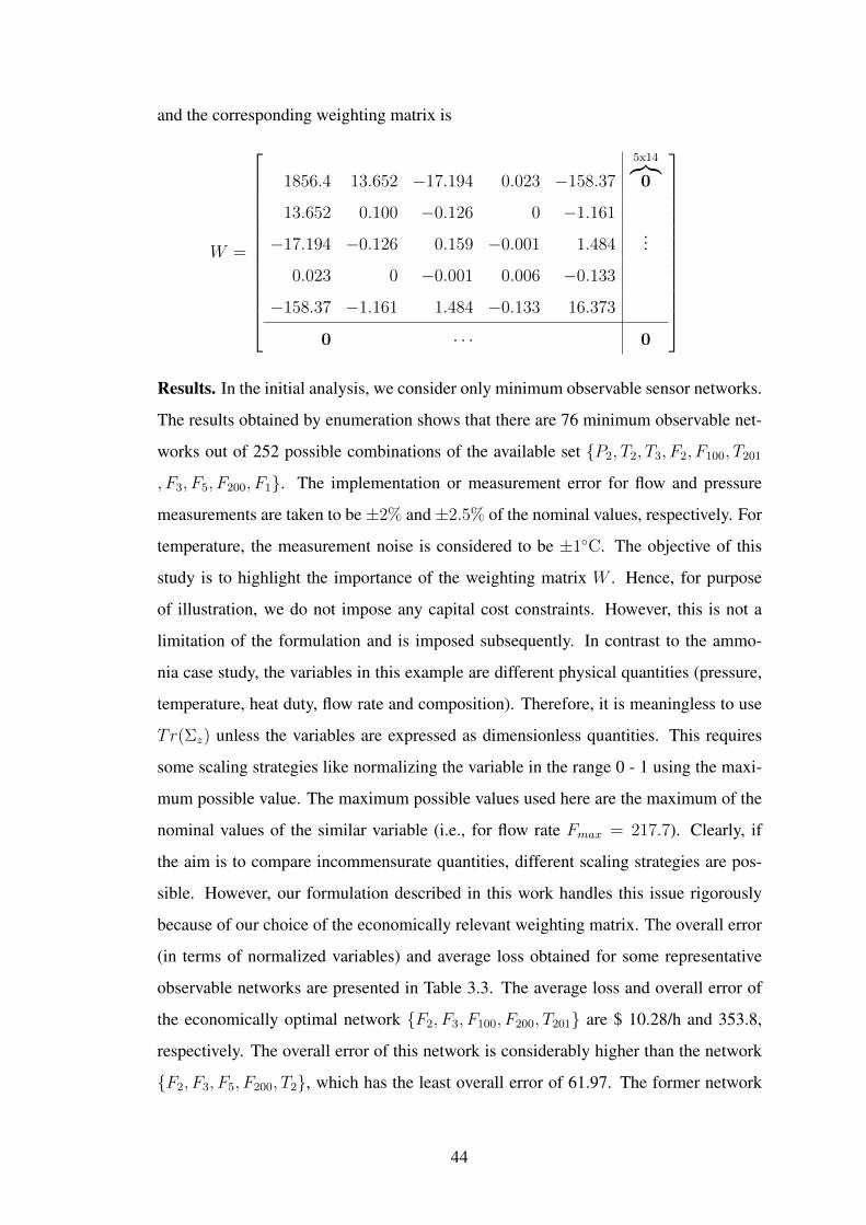
and the corresponding weighting matrix is

W =

1856.4 13.652 −17.194 0.023 −158.37

5x14︷︸︸︷0

13.652 0.100 −0.126 0 −1.161

−17.194 −0.126 0.159 −0.001 1.484...

0.023 0 −0.001 0.006 −0.133

−158.37 −1.161 1.484 −0.133 16.373

0 · · · 0

Results. In the initial analysis, we consider only minimum observable sensor networks.

The results obtained by enumeration shows that there are 76 minimum observable net-

works out of 252 possible combinations of the available set {P2, T2, T3, F2, F100, T201

, F3, F5, F200, F1}. The implementation or measurement error for flow and pressure

measurements are taken to be±2% and±2.5% of the nominal values, respectively. For

temperature, the measurement noise is considered to be ±1◦C. The objective of this

study is to highlight the importance of the weighting matrix W . Hence, for purpose

of illustration, we do not impose any capital cost constraints. However, this is not a

limitation of the formulation and is imposed subsequently. In contrast to the ammo-

nia case study, the variables in this example are different physical quantities (pressure,

temperature, heat duty, flow rate and composition). Therefore, it is meaningless to use

Tr(Σz) unless the variables are expressed as dimensionless quantities. This requires

some scaling strategies like normalizing the variable in the range 0 - 1 using the maxi-

mum possible value. The maximum possible values used here are the maximum of the

nominal values of the similar variable (i.e., for flow rate Fmax = 217.7). Clearly, if

the aim is to compare incommensurate quantities, different scaling strategies are pos-

sible. However, our formulation described in this work handles this issue rigorously

because of our choice of the economically relevant weighting matrix. The overall error

(in terms of normalized variables) and average loss obtained for some representative

observable networks are presented in Table 3.3. The average loss and overall error of

the economically optimal network {F2, F3, F100, F200, T201} are $ 10.28/h and 353.8,

respectively. The overall error of this network is considerably higher than the network

{F2, F3, F5, F200, T2}, which has the least overall error of 61.97. The former network

44

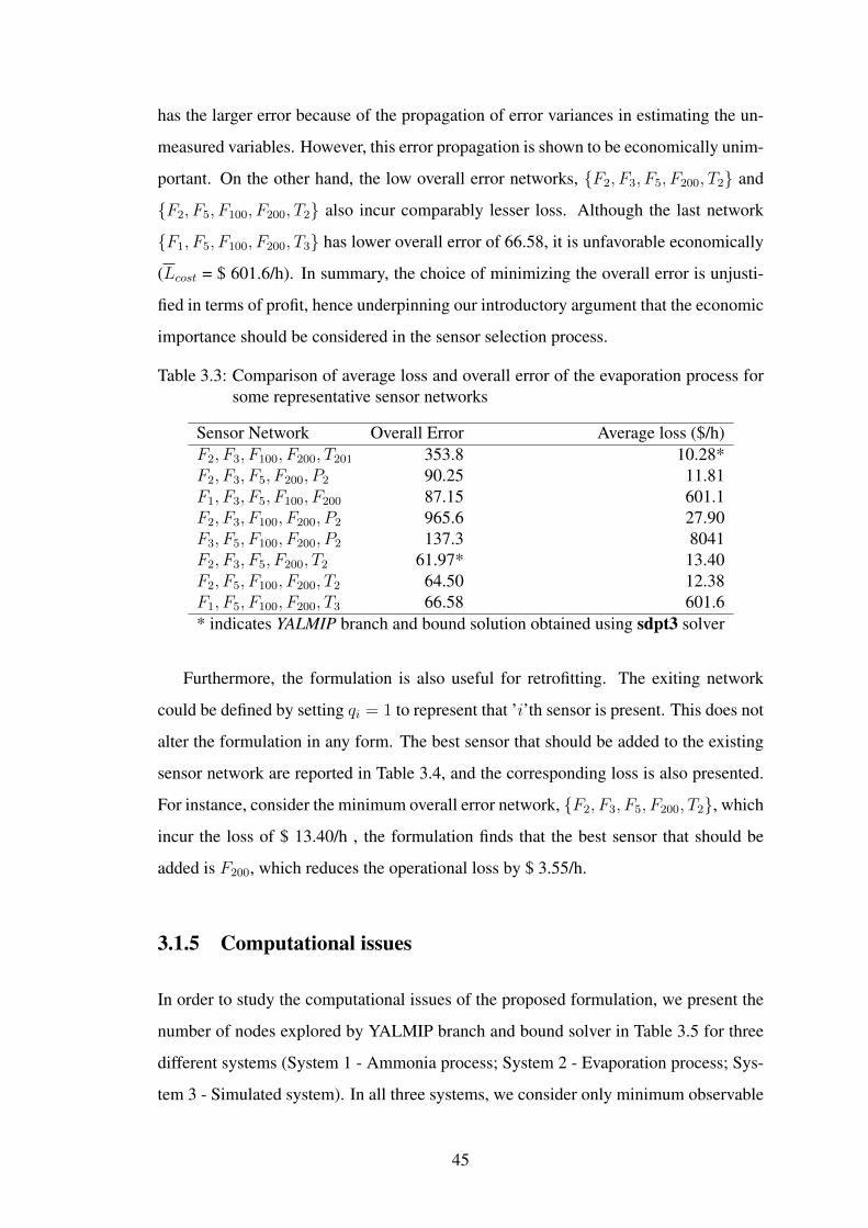
has the larger error because of the propagation of error variances in estimating the un-

measured variables. However, this error propagation is shown to be economically unim-

portant. On the other hand, the low overall error networks, {F2, F3, F5, F200, T2} and

{F2, F5, F100, F200, T2} also incur comparably lesser loss. Although the last network

{F1, F5, F100, F200, T3} has lower overall error of 66.58, it is unfavorable economically

(Lcost = $ 601.6/h). In summary, the choice of minimizing the overall error is unjusti-

fied in terms of profit, hence underpinning our introductory argument that the economic

importance should be considered in the sensor selection process.

Table 3.3: Comparison of average loss and overall error of the evaporation process forsome representative sensor networks

Sensor Network Overall Error Average loss ($/h)F2, F3, F100, F200, T201 353.8 10.28*F2, F3, F5, F200, P2 90.25 11.81F1, F3, F5, F100, F200 87.15 601.1F2, F3, F100, F200, P2 965.6 27.90F3, F5, F100, F200, P2 137.3 8041F2, F3, F5, F200, T2 61.97* 13.40F2, F5, F100, F200, T2 64.50 12.38F1, F5, F100, F200, T3 66.58 601.6* indicates YALMIP branch and bound solution obtained using sdpt3 solver

Furthermore, the formulation is also useful for retrofitting. The exiting network

could be defined by setting qi = 1 to represent that ’i’th sensor is present. This does not

alter the formulation in any form. The best sensor that should be added to the existing

sensor network are reported in Table 3.4, and the corresponding loss is also presented.

For instance, consider the minimum overall error network, {F2, F3, F5, F200, T2}, which

incur the loss of $ 13.40/h , the formulation finds that the best sensor that should be

added is F200, which reduces the operational loss by $ 3.55/h.

3.1.5 Computational issues

In order to study the computational issues of the proposed formulation, we present the

number of nodes explored by YALMIP branch and bound solver in Table 3.5 for three

different systems (System 1 - Ammonia process; System 2 - Evaporation process; Sys-

tem 3 - Simulated system). In all three systems, we consider only minimum observable

45

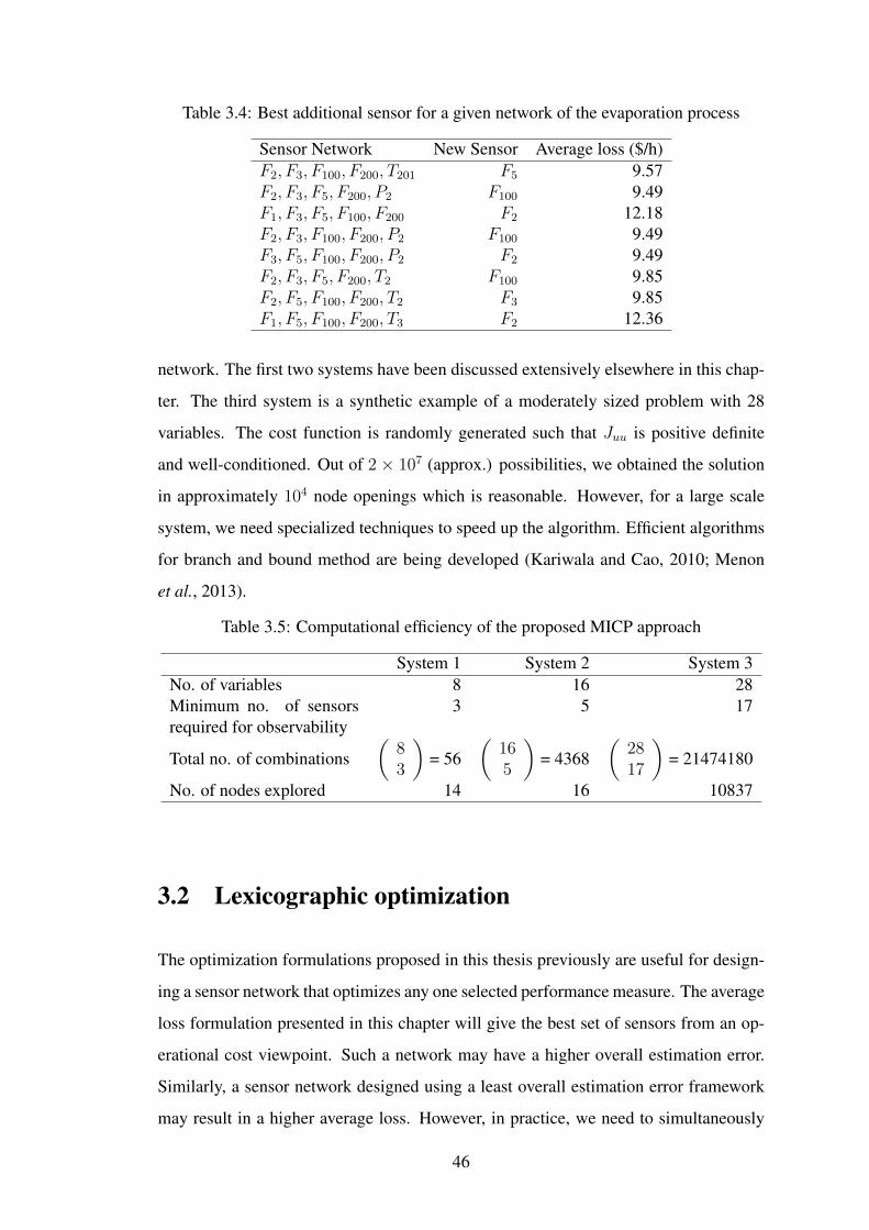
Table 3.4: Best additional sensor for a given network of the evaporation process

Sensor Network New Sensor Average loss ($/h)F2, F3, F100, F200, T201 F5 9.57F2, F3, F5, F200, P2 F100 9.49F1, F3, F5, F100, F200 F2 12.18F2, F3, F100, F200, P2 F100 9.49F3, F5, F100, F200, P2 F2 9.49F2, F3, F5, F200, T2 F100 9.85F2, F5, F100, F200, T2 F3 9.85F1, F5, F100, F200, T3 F2 12.36

network. The first two systems have been discussed extensively elsewhere in this chap-

ter. The third system is a synthetic example of a moderately sized problem with 28

variables. The cost function is randomly generated such that Juu is positive definite

and well-conditioned. Out of 2 × 107 (approx.) possibilities, we obtained the solution

in approximately 104 node openings which is reasonable. However, for a large scale

system, we need specialized techniques to speed up the algorithm. Efficient algorithms

for branch and bound method are being developed (Kariwala and Cao, 2010; Menon

et al., 2013).

Table 3.5: Computational efficiency of the proposed MICP approach

System 1 System 2 System 3No. of variables 8 16 28Minimum no. of sensorsrequired for observability

3 5 17

Total no. of combinations(

83

)= 56

(165

)= 4368

(2817

)= 21474180

No. of nodes explored 14 16 10837

3.2 Lexicographic optimization

The optimization formulations proposed in this thesis previously are useful for design-

ing a sensor network that optimizes any one selected performance measure. The average

loss formulation presented in this chapter will give the best set of sensors from an op-

erational cost viewpoint. Such a network may have a higher overall estimation error.

Similarly, a sensor network designed using a least overall estimation error framework

may result in a higher average loss. However, in practice, we need to simultaneously

46

optimize for both the performance measures. To ameliorate this shortcoming, Baga-

jewicz and Sánchez (2000) presented a minimum cost model for the design of reliable

sensor networks. This was accomplished by minimizing the sensor cost while ensur-

ing reliability of some or all variables above a pre-specified threshold values. They

also demonstrated the cases wherein sensor network design procedure was carried out

with pre-specified threshold values for other measures such as error variances and es-

timability. However, satisfying threshold values do not optimize for the performance

measures.

Alternately, one could rank or prioritize the objectives and solve for them in an

orderly way. In this approach, the objective with the highest priority is optimized first.

With the optimal value of the first objective being set as an equality constraint, the

objective with the second highest priority is optimized. Now, with the optimal function

values of the first two objectives being set as equality constraints, the next prioritized

objective is optimized and so on. In other words, the multiobjective problem is solved in

lexicographic sense. Equivalently, this problem could be cast as a one-step optimization

problem by combining all the objective functions into a single objective function with

the proper choice of weights for each of the objective based on the assumed priority

level (Sherali, 1982). Following similar approach, Bhushan and Rengaswamy (2002a)

presented a way of combining the objective of maximizing reliability with (minimizing)

sensor cost. Later, Bhushan et al. (2008) presented the sensor selection problem that

were not only reliable and cost optimal but also robust to uncertainties in the underlying

model and probability of sensor failure data. They combined the objectives to solve

the problem in lexicographic sense using the algorithm proposed by (Sherali, 1982) to

obtain the corresponding weights for each of the objective function.

In this section, our focus is to address the sensor network design problem that will

minimize both the average loss and overall error in the lexicographic sense. Here we

treat average loss as the primary objective and overall estimation error as our secondary

47

objective. Now, the optimization formulation can be expressed as

minqi,tc,Yc,te,Ye

L =1

2λ1tc + λ2te (3.32a)

s.t. T r(Yc) ≤ tc (3.32b) Yc RTC

(RTC)T

(CTQC)

� 0 (3.32c)

Tr(Ye) ≤ te (3.32d) Ye C

CT (CTQC)

� 0 (3.32e)

qi ∈ {0, 1} (3.32f)

Q = diag{ qiσi2} (3.32g)

nz∑i=1

ciqi ≤ c∗ (3.32h)

The resulting formulation preserves the mixed integer cone programming formu-

lation presented in the previous section. The constraints (3.32b)-(3.32c) correspond

to the minimum loss framework whereas the constraints (3.32d)-(3.32e) correspond to

minimum error framework.

The most crucial step in this formulation is selecting the appropriate weights, λ1

and λ2. In this work, we select the weights using Algorithm 2 of Sherali (1982). Re-

call that our primary objective is minimizing average loss, therefore, we set the value

of λ1 = (1 + M) and λ2 = 1, where M is the maximum possible value among all

feasible solutions of the minimum error formulation and M > 0. For the case of two

different objectives, f1(q) and f2(q), the appropriate choice of a single parameter will

render the lexicographic solution and the value of M used here can be interpreted as

the maximum possible relative change in the value of primary cost function for a mini-

mal change in the secondary cost function value. According to Algorithm 2 of Sherali

(1982), the value of M is chosen as the upper bound on loss value. The idea behind

such a choice is that λ1f1(q) > λ2f2(q) for any solution q. However, if there is one

feasible solution q′ such that f1(q′) > f2(q′), then one can choose the value of M to be

f1(q′) because minimization of (1 + f1(q′))f1(q) > f2(q) if f1(q) > 1 and f2(q) > 1

48

for any q. The conditions, f1(q) > 1 and f2(q) > 1, can be easily tested by selecting all

the sensors and evaluating the analytical expressions available for f1(q) = Tr(Σz(q))

and f2(q) = Tr(WΣz(q)). If this is true, then the subset of q will also satisfy the

above condition. On the other hand, if the feasible solution q′ satisfies f2(q′) > f1(q′),

then one can choose the value of M to be f2(q′) following similar arguments. In sum-

mary, if a feasible solution has been determined, then the value of M can be taken as

max(f1(q′), f2(q′)). Now, it is important to notice that the set of primary variables is

one of the feasible solution. Therefore, we could approximate the value of M to be

the overall error obtained using primary variables as candidate measurements assuming

the conditions presented above are valid. This framework could be easily modified to

consider overall estimation error as primary objective and average loss as secondary

objective.

3.2.1 Illustration: Simple ammonia process

In this section, our objective is to demonstrate the lexicographic approach of designing

sensor network to minimize both the average loss and overall error. For this purpose,

let us revisit the flow network of a simplified ammonia process discussed in subsec-

tion 3.1.3 and the system is depicted in Figure 2.3. For the purpose of demonstration,

we only consider minimum observable sensor networks. In Table 3.1, we presented

the results obtained by our formulation and also those obtained by explicit enumeration

of all observable solutions. Notice that the minimum average loss network was found

to be {F1, F5, F8} but it has the highest overall error. On the other hand, there are

12 other economically optimal sensor networks with better overall error value than the

sensor network {F1, F5, F8} . Therefore, this necessitates the importance of minimizing

overall error along with the average loss function. Hence, we propose to use the lexi-

cographic approach of solving multi-objective optimization problems. The value of M

is set to be 11 based on the chosen primary variables . The lexicographic solution was

found to be {F2, F6, F8} which incurs an average loss of $ 3 /h and the overall error is

12. This overall error value is better than that of the sensor network {F1, F5, F8} which

had the error value of 16.

49

3.3 Summary

This chapter addressed the issue of obtaining the economically optimal sensor network

in the presence of uncertainty caused by measurement error. The procedure relates

process economics and estimation accuracy by determining the loss caused due to un-

certainty in measurements. The analytical solution for the loss function showing the

economic importance has been achieved by the proper choice of a weighting matrix.

It is proper in the sense that cost function has been defined using economics of the

process. This analysis helps the design engineer to quickly evaluate between the al-

ternatives and choose the optimal network. The solution strategy is also presented to

convert the MINLP into a mixed integer cone program which can be solved to global

optimality. Finally, we discussed the lexicographic optimization framework to obtain

the minimum loss sensor network that also minimizes the overall error of the network.

50

CHAPTER 4

ROBUST OPTIMAL SENSOR NETWORK DESIGN

Partly based on the paper presented in 11th International Symposium on Process

Systems Engineering

In this chapter, we extend our sensor network design procedure that addressed data

reconciliation, to handle sensor faults scenarios. It is assumed here that only one sensor

can fail at a time. Sensor failure situations can be handled by increasing the redundancy

of the network. Therefore, the primary aim of this chapter is to determine a redundant

set of sensors that will retain observability of the system in case of sensor failures. In

other words, the resulting network should be robust to sensor failures. To address this,

we propose a scenario based optimization formulation that finds a robust optimal sensor

network by minimizing the average loss function subject to satisfying observability

conditions for each sensor failure scenarios. Although such a robust sensor network

will result in an observable sub-network in case of sensor failure, the sub-network need

not be optimal. Therefore, we also extend the formulation to determine the robust

optimal sensor network by minimizing the worst-case loss function.

4.1 Introduction

To achieve effective monitoring, control and fault diagnosis of chemical processes, re-

liable measurements of process variables must be available. Sensor networks designed

for the purpose of process monitoring should provide a good estimate of process vari-

ables. In this regard, the data reconciliation framework allows us to determine the sen-

sor network that will provide precise estimates of the process variables. In the previous

chapter, we intended to find a sensor network based on monetary value such that the op-

erational loss caused due to measurement errors was minimized. However, sensors are

prone to faults like bias, drift or complete failure, etc. This will eventually degrade the

performance, demand process shutdown or even cause fatal accidents. Therefore, the

sensor network we design should be robust enough to handle sensor failure situations.

The desirable property of a sensor network, to handle actual sensor failure situa-

tions, is redundancy. This could be achieved either by adding more sensors to measure

the same variables (hardware redundancy) or by measuring additional variables such

that there are multiple ways of estimating the process variables using process model

(analytical or spatial redundancy). Since adding multiple sensors is costly, our focus

is to exploit analytical redundancy to obtain a redundant sensor network. Some of the

previous works that addressed the sensor network design procedure related to sensor

fault situations and redundant measurement selection were reviewed in Chapter 2. Re-

call that a sensor network design procedure based on maximizing system reliability will

maximizes the probability of estimating process variables, when sensors are likely to

fail. Though such a design may presumably reduce the sensor fault occurrence, it will

not be useful in case of actual sensor faults, because of its inability to obtain the esti-

mate of unmeasured variables. However, this metric is not readily deciphered by the

designers, as discussed earlier. Hence, our current focus is to design an economically

optimal sensor network that can handle sensor failure situations.

This chapter is organized as follows: First, we enforce the property of system re-

dundancy to design a reliable or robust sensor network that is capable of observing all

the process variables even in case of sensor failures. This system redundancy property

is utilized within the framework of minimum loss formulation presented in the previous

chapters. Next, we present the modified optimization formulation that addresses the

problem of robust optimal sensor network design by minimizing the worst case loss in

case of sensor failures. Finally, illustrations are provided to demonstrate the approach.

4.2 Robust optimal sensor network design: Average loss

formulation

The sensor network we design should be capable of providing a good estimate of the

unmeasured variables, should be able to detect and identify faults, and also be robust

52

to uncertainties such as process faults and sensor faults, etc. The choice of a redundant

sensor network plays a vital role in identifying instrument faults, in aiding us to observe

the process variables under sensor fault conditions by exploiting analytical redundancy,

and also improving the estimates through data reconciliation. It is important to note

that analytical redundancy (that is, the use of redundancy through the use of models)

cannot be increased unless new instrumentation is added. Therefore, the objective of

this section is to make a clever choice on the set of redundant measurements that are not

only useful in improving the estimates but also help us to estimate all the unmeasured

variables and measured variables for which the sensors have failed. In other words, we

focus on designing the sensor network that will improve the analytical redundancy.

Bagajewicz (1997) defined robustness as the ability of a sensor network to detect

gross errors (error detectability), provide results at a certain level of precision in the

presence of gross errors (availability), and minimize corruption of data by undetected

gross errors (resilience). In this work, we assume a suitable fault detection and main-

tenance policy is in place to identify sensor faults and take corrective action. Also,

we assume that the data reconciliation is then performed, eliminating the faulty mea-

surements. Hence, our scope is to design a suitable set of redundant measurements that

possesses a certain level of analytical redundancy, to be useful in case of sensor failures.

DEFINITION 4.1 The sensor network is said to be robust if the network is redundant

and in addition, all the process variables should be estimable by ‘more than k’ different

means to account for k sensors failing at a time.

EXAMPLE 4.1

The purpose of this example is to illustrate the idea of robust sensor network to single

sensor failure situations. For the case of single sensor failing at a time, there should be

atleast two ways of estimating all the variables. Consider the system with three process

units and six streams as depicted in Figure 4.1.

The minimum number of independent sensors required for the system to be observ-

able under normal operating conditions is three. Recall from Example 2.1 that the sen-

sor network {F1, F2, F4} is observable and the network {F1, F2, F3} is unobservable.

The minimum observable sensor network is non-redundant. For a non-redundant sen-

53

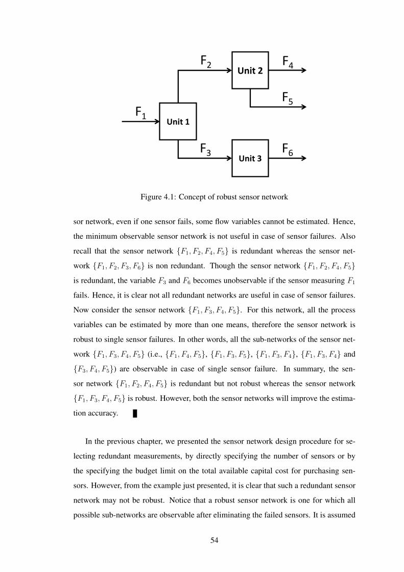
Unit 2

Unit 3

Unit 1F1

F2

F3

F4

F5

F6

Figure 4.1: Concept of robust sensor network

sor network, even if one sensor fails, some flow variables cannot be estimated. Hence,

the minimum observable sensor network is not useful in case of sensor failures. Also

recall that the sensor network {F1, F2, F4, F5} is redundant whereas the sensor net-

work {F1, F2, F3, F6} is non redundant. Though the sensor network {F1, F2, F4, F5}

is redundant, the variable F3 and F6 becomes unobservable if the sensor measuring F1

fails. Hence, it is clear not all redundant networks are useful in case of sensor failures.

Now consider the sensor network {F1, F3, F4, F5}. For this network, all the process

variables can be estimated by more than one means, therefore the sensor network is

robust to single sensor failures. In other words, all the sub-networks of the sensor net-

work {F1, F3, F4, F5} (i.e., {F1, F4, F5}, {F1, F3, F5}, {F1, F3, F4}, {F1, F3, F4} and

{F3, F4, F5}) are observable in case of single sensor failure. In summary, the sen-

sor network {F1, F2, F4, F5} is redundant but not robust whereas the sensor network

{F1, F3, F4, F5} is robust. However, both the sensor networks will improve the estima-

tion accuracy.

In the previous chapter, we presented the sensor network design procedure for se-

lecting redundant measurements, by directly specifying the number of sensors or by

the specifying the budget limit on the total available capital cost for purchasing sen-

sors. However, from the example just presented, it is clear that such a redundant sensor

network may not be robust. Notice that a robust sensor network is one for which all

possible sub-networks are observable after eliminating the failed sensors. It is assumed

54

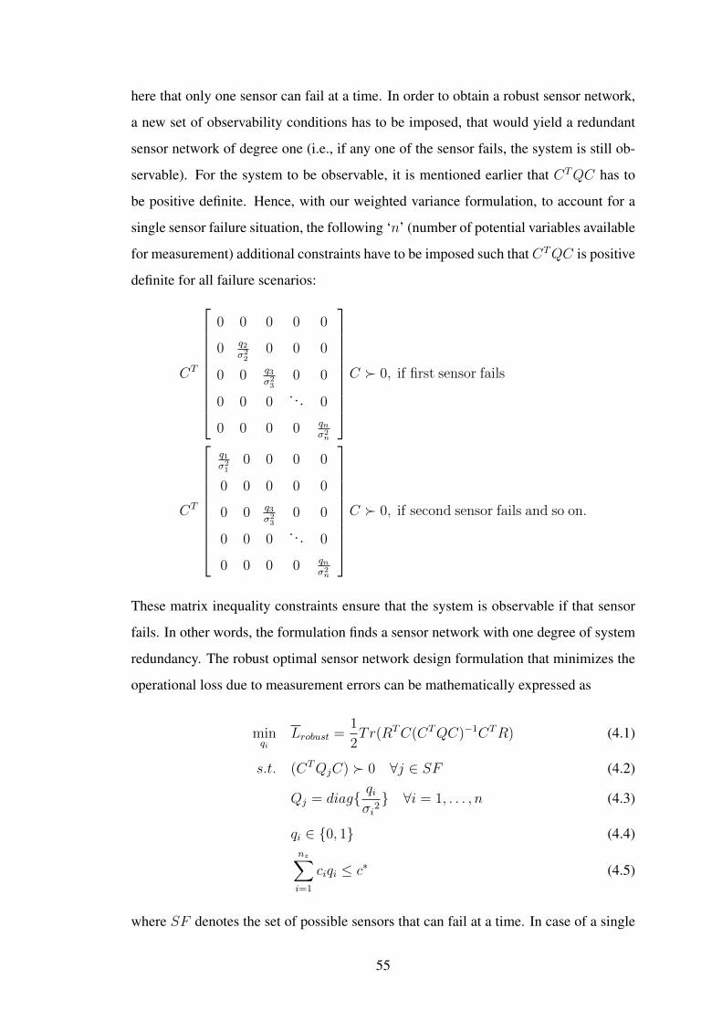
here that only one sensor can fail at a time. In order to obtain a robust sensor network,

a new set of observability conditions has to be imposed, that would yield a redundant

sensor network of degree one (i.e., if any one of the sensor fails, the system is still ob-

servable). For the system to be observable, it is mentioned earlier that CTQC has to

be positive definite. Hence, with our weighted variance formulation, to account for a

single sensor failure situation, the following ‘n’ (number of potential variables available

for measurement) additional constraints have to be imposed such that CTQC is positive

definite for all failure scenarios:

CT

0 0 0 0 0

0 q2σ22

0 0 0

0 0 q3σ23

0 0

0 0 0. . . 0

0 0 0 0 qnσ2n

C � 0, if first sensor fails

CT

q1σ21

0 0 0 0

0 0 0 0 0

0 0 q3σ23

0 0

0 0 0. . . 0

0 0 0 0 qnσ2n

C � 0, if second sensor fails and so on.

These matrix inequality constraints ensure that the system is observable if that sensor

fails. In other words, the formulation finds a sensor network with one degree of system

redundancy. The robust optimal sensor network design formulation that minimizes the

operational loss due to measurement errors can be mathematically expressed as

minqi

Lrobust =1

2Tr(RTC(CTQC)−1CTR) (4.1)

s.t. (CTQjC) � 0 ∀j ∈ SF (4.2)

Qj = diag{ qiσi2} ∀i = 1, . . . , n (4.3)

qi ∈ {0, 1} (4.4)nz∑i=1

ciqi ≤ c∗ (4.5)

where SF denotes the set of possible sensors that can fail at a time. In case of a single

55

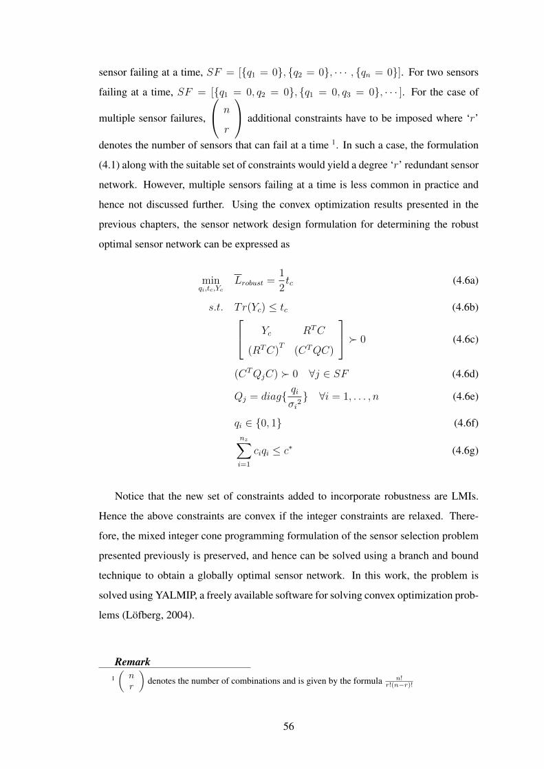
sensor failing at a time, SF = [{q1 = 0}, {q2 = 0}, · · · , {qn = 0}]. For two sensors

failing at a time, SF = [{q1 = 0, q2 = 0}, {q1 = 0, q3 = 0}, · · · ]. For the case of

multiple sensor failures,

n

r

additional constraints have to be imposed where ‘r’

denotes the number of sensors that can fail at a time 1. In such a case, the formulation

(4.1) along with the suitable set of constraints would yield a degree ‘r’ redundant sensor

network. However, multiple sensors failing at a time is less common in practice and

hence not discussed further. Using the convex optimization results presented in the

previous chapters, the sensor network design formulation for determining the robust

optimal sensor network can be expressed as

minqi,tc,Yc

Lrobust =1

2tc (4.6a)

s.t. T r(Yc) ≤ tc (4.6b) Yc RTC

(RTC)T

(CTQC)

� 0 (4.6c)

(CTQjC) � 0 ∀j ∈ SF (4.6d)

Qj = diag{ qiσi2} ∀i = 1, . . . , n (4.6e)

qi ∈ {0, 1} (4.6f)nz∑i=1

ciqi ≤ c∗ (4.6g)

Notice that the new set of constraints added to incorporate robustness are LMIs.

Hence the above constraints are convex if the integer constraints are relaxed. There-

fore, the mixed integer cone programming formulation of the sensor selection problem

presented previously is preserved, and hence can be solved using a branch and bound

technique to obtain a globally optimal sensor network. In this work, the problem is

solved using YALMIP, a freely available software for solving convex optimization prob-

lems (Löfberg, 2004).

Remark1(

nr

)denotes the number of combinations and is given by the formula n!

r!(n−r)!

56

The term robust sensor network defined in this section is related to the conceptof estimability of the variables presented in Bagajewicz and Sánchez (1999). Forthe case of single sensor failure scenario, the robust sensor network is equivalentto demanding the estimability of all the variable being strictly greater than oneor setting the inequality as greater than or equal to two. However, the concept ofestimability requires one to generate the possible cutsets of a graph a priori andin addition, the overall optimization formulation resulted in an MINLP whichdoes not guarantee global optimality. On the other hand, in our formulation westate the sensor failure scenarios as LMIs and hence it can be solved to globaloptimality efficiently.

4.2.1 Illustration: Evaporation process

Consider the forced circulation evaporation process discussed in Section 3.1.4. Recall

that the process model has five degrees of freedom assuming the active constraints are

enforced. Therefore, at least five variables have to be measured for the system to be

observable for data reconciliation. However, if any of the sensors fail then the system

is always unobservable. Hence, a redundant sensor network of at least degree one is

required to handle a single sensor failing at a time.

First, we consider the sensor selection problem given the budget limit for purchasing

sensors. In order to consider the effect of capital cost constraint, the cost of flow, tem-

perature and pressure sensors are assumed to be $ 100 , $ 150 and $ 200 respectively.

This constraint limits the number of sensors to be selected based on the available cap-

ital cost c∗. The economically optimal networks for different available capital cost are

presented in Table 4.1. For the available cost of $ 500 , it is trivial to see that only flow

sensors could be selected as they form a minimum observable network which cause the

average loss of $ 12.2/h. With extra $ 50 of available resource, we obtain a different

optimal network {F2, F3, F100, F200, T201} which corresponds to the loss of $ 10.28/h.

It is important to recall that this network is also the optimal minimum observable net-

work with equal sensor costs. With further increase in available capital cost, we obtain

redundant networks, as redundant measurements improve the estimation accuracy and

hence reduces the operational loss due to measurement uncertainty.

Now we compare the results of sensor network design formulation for two cases:

without and with sensor failure conditions. The corresponding economically optimal

57

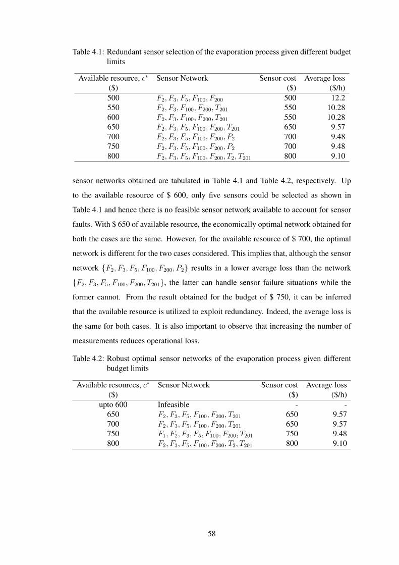
Table 4.1: Redundant sensor selection of the evaporation process given different budgetlimits

Available resource, c∗ Sensor Network Sensor cost Average loss($) ($) ($/h)500 F2, F3, F5, F100, F200 500 12.2550 F2, F3, F100, F200, T201 550 10.28600 F2, F3, F100, F200, T201 550 10.28650 F2, F3, F5, F100, F200, T201 650 9.57700 F2, F3, F5, F100, F200, P2 700 9.48750 F2, F3, F5, F100, F200, P2 700 9.48800 F2, F3, F5, F100, F200, T2, T201 800 9.10

sensor networks obtained are tabulated in Table 4.1 and Table 4.2, respectively. Up

to the available resource of $ 600, only five sensors could be selected as shown in

Table 4.1 and hence there is no feasible sensor network available to account for sensor

faults. With $ 650 of available resource, the economically optimal network obtained for

both the cases are the same. However, for the available resource of $ 700, the optimal

network is different for the two cases considered. This implies that, although the sensor

network {F2, F3, F5, F100, F200, P2} results in a lower average loss than the network

{F2, F3, F5, F100, F200, T201}, the latter can handle sensor failure situations while the

former cannot. From the result obtained for the budget of $ 750, it can be inferred

that the available resource is utilized to exploit redundancy. Indeed, the average loss is

the same for both cases. It is also important to observe that increasing the number of

measurements reduces operational loss.

Table 4.2: Robust optimal sensor networks of the evaporation process given differentbudget limits

Available resources, c∗ Sensor Network Sensor cost Average loss($) ($) ($/h)

upto 600 Infeasible - -650 F2, F3, F5, F100, F200, T201 650 9.57700 F2, F3, F5, F100, F200, T201 650 9.57750 F1, F2, F3, F5, F100, F200, T201 750 9.48800 F2, F3, F5, F100, F200, T2, T201 800 9.10

58

4.3 Robust optimal sensor network design: Worst-case

average loss formulation

In the previous section, we presented the sensor network design formulation that min-

imized the average loss function for selecting the redundant measurements that are ro-

bust to handle sensor failures. This was accomplished by specifying the observability

conditions for each sensor failure situation. Although such a robust sensor network will

result in an observable sub-network in case of sensor failure, the sub-network need not

be optimal. Therefore, the current objective is to determine the robust sensor network

that minimizes the average loss function among all observable sub-networks. In other

words, our focus is on determining the redundant sensor network that minimizes the

maximum average loss in case of sensor failure situations. It is important to recall that

the term average loss signifies the monetary loss one would incur because of the pres-

ence of measurement errors. Also notice that the value of average loss represents the

loss in profit due to measurement errors only and does not account for the actual loss

we incur in the event sensor failure, however, the sensor network will still be observ-

able in case of sensor failures. Hence we define the term worst-case average loss as the

maximum possible monetary loss due to measurement errors in the event of any sensor

sensor failing at a time of the designed sensor network. Therefore, in order to reduce

the average loss we incur in case of sensor failure, we need to determine the sensor

network by minimizing the worst-case average loss function.

Mathematically, the problem could be stated as:

minqi∈{0,1}

maxj∈SF

L = 12Tr(RTC(CTQC)−1CTR) (4.7)

where Q = diag{ qiσi2} and SF denotes the set of possible sensors that can fail at a time.

In case of a single sensor failing at a time, SF = [{q1 = 0}, {q2 = 0}, · · · , {qn = 0}].

For two sensors failing at a time, SF = [{q1 = 0, q2 = 0}, {q1 = 0, q3 = 0}, · · · ]. In

other words, SF is a set that contains all possible sensor failure scenarios. The min-

max formulation is a non-linear integer programming problem. However, expressing

59

the above problem in epigraph form for all possible scenarios, we obtain

minqi,tc,Yc,j

Lrobust,wc =1

2tc (4.8a)

s.t. T r(Yc,j) ≤ tc (4.8b) Yc,j RTC

(RTC)T

(CTQjC)

� 0 ∀j ∈ SF (4.8c)

Qj = diag{ qiσi2} ∀i = 1, . . . , n (4.8d)

qi ∈ {0, 1} (4.8e)nz∑i=1

ciqi ≤ c∗ (4.8f)

where matrix variables, Yc,j’s are the internal variables created during convexification

for each of the sensor failure scenarios. The final formulation is a mixed integer conic

problem. The linear relaxation of the integer constraints result in a convex formulation,

hence preserving convexity of our original formulation. This can be readily solved to

global optimality using branch and bound algorithms.

4.3.1 Illustration: Evaporation process

Let us revisit the forced circulation evaporation process presented previously in the

context of robust optimal sensor selection by minimizing average loss function. Recall

that for the system to be observable, we need to measure at least five variables. Further

recall that to handle sensor failure events, we need to identify the sensor network of at

least system redundancy of degree one. Now, we illustrate the sensor selection problem

that minimizes the worst case average loss function.

Let us assume the cost of flow, temperature and pressure sensors to be $ 100, $

150 and $ 200, respectively, to show the effect of available monetary resource. The

robust optimal sensor networks obtained for different budget limits are tabulated in Ta-

ble 4.3. Up to the available resource of $ 600, only five sensors could be selected

as shown in Table 4.2 and hence there is no feasible sensor network available to ac-

count for sensor faults. With $ 650 of available capital cost, the robust optimal net-

60

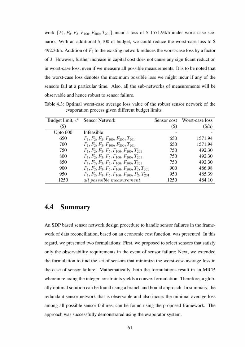
work {F1, F2, F3, F100, F200, T201} incur a loss of $ 1571.94/h under worst-case sce-

nario. With an additional $ 100 of budget, we could reduce the worst-case loss to $

492.30/h. Addition of F5 to the existing network reduces the worst-case loss by a factor

of 3. However, further increase in capital cost does not cause any significant reduction

in worst-case loss, even if we measure all possible measurements. It is to be noted that

the worst-case loss denotes the maximum possible loss we might incur if any of the

sensors fail at a particular time. Also, all the sub-networks of measurements will be

observable and hence robust to sensor failure.

Table 4.3: Optimal worst-case average loss value of the robust sensor network of theevaporation process given different budget limits

Budget limit, c∗ Sensor Network Sensor cost Worst-case loss($) ($) ($/h)

Upto 600 Infeasible - -650 F1, F2, F3, F100, F200, T201 650 1571.94700 F1, F2, F3, F100, F200, T201 650 1571.94750 F1, F2, F3, F5, F100, F200, T201 750 492.30800 F1, F2, F3, F5, F100, F200, T201 750 492.30850 F1, F2, F3, F5, F100, F200, T201 750 492.30900 F1, F2, F3, F5, F100, F200, T2, T201 900 486.98950 F1, F2, F3, F5, F100, F200, P2, T201 950 485.39

1250 all posssible measurement 1250 484.10

4.4 Summary

An SDP based sensor network design procedure to handle sensor failures in the frame-

work of data reconciliation, based on an economic cost function, was presented. In this

regard, we presented two formulations: First, we proposed to select sensors that satisfy

only the observability requirements in the event of sensor failure; Next, we extended

the formulation to find the set of sensors that minimize the worst-case average loss in

the case of sensor failure. Mathematically, both the formulations result in an MICP,

wherein relaxing the integer constraints yields a convex formulation. Therefore, a glob-

ally optimal solution can be found using a branch and bound approach. In summary, the

redundant sensor network that is observable and also incurs the minimal average loss

among all possible sensor failures, can be found using the proposed framework. The

approach was successfully demonstrated using the evaporator system.

61

CHAPTER 5

PROFITABLE AND DYNAMICALLY FEASIBLE

OPERATING POINT SELECTION FOR

CONSTRAINED PROCESSES

Based on the paper published in Journal of Process Control

The operating point of a typical chemical process is determined by solving a non-

linear optimization problem where the objective is to minimize an economic cost subject

to constraints. Often, some or all of the constraints at the optimal solution are active,

i.e., the solution is constrained. Though it is profitable to operate at the constrained

optimal point, it might lead to infeasible operation due to uncertainties. Hence, indus-

tries try to operate the plant close to the optimal point by “backing-off” to achieve the

desired economic benefits. Therefore, the primary focus of this chapter is to present an

optimization formulation for solving the dynamic back-off problem based on an eco-

nomic cost function. In this regard, we work within a stochastic framework that ensures

feasible dynamic operating region within the prescribed confidence limit. In this work,

we aim to reduce the economic loss due to the back-off by simultaneously solving for

the operating point and a compatible controller that ensures feasibility. Since the result-

ing formulation is non-linear and non-convex, we propose a novel two-stage iterative

solution procedure such that a convex problem is solved at each step in the iteration.

Finally, the proposed approach is demonstrated using case studies.

5.1 Introduction

Profitability is the major concern of the plant operator and one approach to achieve this

is to operate the plant at the optimal point obtained by solving a (typically nonlinear)

steady state optimization problem. The optimizer minimizes a suitable cost function

subject to equality and inequality constraints. Often, the solution of the optimizer is

constrained at some of the inequalities, that is, there are several active constraints. Typ-

ically, it is assumed that these active constraints should be controlled at their limiting

values to achieve economic benefits. However, the presence of uncertainties in the form

of measurement noise, modeling error, parametric uncertainties and disturbances might

cause constraint violations. Therefore, it is important to find an operating point close

to the active constraints such that the plant remains feasible for the expected range of

uncertainties. Thus, the focus of our work is to propose an optimization formulation

that obtains the best trading-off between feasibility and profitability.

Optimal process operations depend on process design and safety thresholds, etc.

These constraints define the feasible operating window to the optimizer. To ensure

feasible operation under uncertain conditions, it may be necessary to “back-off” from

the active constraints which however results in loss of achievable profit. Hence, the

optimizer minimizes a loss function for backing-off from the active constraints. The

term “back-off” is defined as,

Back − off = |Actual steady state operating point

−Nominally optimal steady state operating point| (5.1)

Based on the notion of back-off, Narraway et al. (1991) presented a method to assess

the economic performance of the plant in the presence of disturbances. To ensure feasi-

bility, the maximum amplitude of the disturbance for a certain range of frequency was

used to determine the necessary back-off and alternate designs were evaluated. They

assume the set of measurements are perfectly controlled and controllability is tested

after obtaining the solution. Later, Narraway and Perkins (1993) extended their fre-

quency response based method of estimating the closed loop constraint back off on the

assumption of perfect control hypothesis to select the optimal set of measurements and

manipulated inputs. This was accomplished by introducing the binary decision variable

into the bounds of all possible measurements and manipulations. Also, the method was

extended for the case of realistic PI controllers. Although the formulation is an MILP,

the dimension of the problem is very high owing to the number of frequencies consid-

ered for each of the constraints. To solve this, a solution algorithm was presented where

64

the obtained solution is compared with the open loop (without control) solution to quan-

tify the profitability that would achieved by the controller and the controller with less

benefits are eliminated (Heath et al., 2000). All of the above methods were developed

to handle single disturbance only.

To address the case of multiple disturbances, Bahri et al. (1996) addressed the back

off problem for control of active constraints in the regulatory layer by solving the open

loop problem. Figueroa et al. (1996) extended the above approach to the closed-loop

case where the figure of merit “maximum percentage recovery” is defined to choose

between alternative control configurations. In summary, disturbance is the only source

of uncertainty considered in evaluating the different control structures. However, in

some cases measurement noise and control error also play a significant role.

Disturbances are typically categorized based on the time scale or frequency of oc-

currence as fast or high-frequency disturbance and slow or low-frequency disturbance.

The lower regulatory layer generally handles the fast disturbances whereas the slow dis-

turbances are handled by the steady state optimizer. The objective of the optimization

layer is to provide set points to the control layer. These set points depend on the set of

design variables and measurements selected for estimating the model parameters. And,

the choice of measurements have a profound impact in the steady state economics. In

this regard, de Hennin et al. (1994) presented a method for estimating the likely eco-

nomic benefit that could be achieved by implementing a steady state optimizer. The

cost of instrumentation is also included in addition to the operational cost to determine

the best optimal measurements.

Alternatively, Govatsmark and Skogestad (2005) presented the weighted-cost for-

mulation to determine a robust set-point by enforcing a finite set of disturbance values

in contrast to the maximum expected values of the disturbance vector. However, the

determined set-points might be too conservative and they are indeed affected by the

structural decisions such as control structure, type of controller, choice of manipulated,

controlled and measured variables, etc. Loeblein and Perkins (1998) proposed a mea-

sure of average deviation from optimum that allows the estimation of economic value

of different online optimization structures. In addition to measurement selection, their

work addressed the impact of model uncertainty on the economics of the optimizer.

65

To analyze this issue, the authors considered a simple model, approximate model and

rigorous model and concluded that approximate model is appropriate for on-line op-

timization. Later, Loeblein and Perkins (1999a,b) extended their method of average

deviation from optimum to analyze the dynamic economics of regulatory layer which is

assumed to be implemented using MPC framework. However, fixed control structures

are assumed to rank between the alternatives. Several other authors have addressed

the role of process economics on control structure selection (Bahri et al., 1995, 1996;

Kookos and Perkins, 2002; Kookos, 2005; Young et al., 1996).

Peng et al. (2005) proposed a stochastic formulation for the determination of back-

off points based on the notion of expected dynamic operating region. The basic idea in

their approach is that the simultaneous selection of controller and back off point will

find a optimal controller that minimizes the variability of the active constrained vari-

ables. Since the disturbances are assumed to be stochastic, the dynamic operation is

defined in terms of variance. Extensions of the method to discrete time and partial state

information case do not alter the formulation. Despite this, the final form of the opti-

mization problem contains a set of reverse convex constraints which make the problem

difficult to solve. Therefore, a branch and bound type algorithm was proposed. Sensor

selection for control purposes are addressed in this framework (Peng and Chmielewski,

2005). Chmielewski and Manthanwar (2004) have found that the obtained optimal mul-

tivariable feedback controller can be used to tune the objective function weights of the

MPC controller.

In this work, we propose a stochastic formulation of the dynamic back-off problem

that ensures feasible operation for the prescribed confidence limit. Following Peng et al.

(2005), the dynamic operating region is defined for the given disturbances which follow

from the closed loop covariance analysis of the state space model of the process. The

loss function, is a measure of departure from optimality and we develop a theoretically

and conceptually sound loss function. Controller selection also plays a crucial role

in shaping the dynamic operating region while the size of the region is characterized

by the prescribed confidence limit and variance of the disturbance considered. Thus,

consideration of the controller gain as a decision variable is important in determining

the optimal operating point which minimizes the loss in profit. Therefore, the focus

66

of our work is to propose an optimization formulation that determines the economic

backed-off operating point by finding at the same time a suitable controller gain.

The current formulation contains an explicit representation of the ellipsoid to de-

scribe the system dynamics and can handle partially constrained cases. The formu-

lation presents a back-off term as slack variable in terms of the respective variances.

Furthermore, a novel solution methodology has been presented to solve the non-linear

non-convex problem.

This chapter is organized as follows. In the next section, we define the problem

and present a development of stochastic formulation and convex relaxations of the con-

straints. Next, a solution algorithm has been developed. Finally, illustrations are pro-

vided to demonstrate the approach.

5.2 Formulation of dynamic back-off problem

The objective of this section is to present an optimization formulation that determines

the most profitable steady state operating point given that the plant has to remain feasi-

ble for the expected set of disturbances affecting the process. Hence, the optimization

formulation should also include differential constraints that characterize the dynamic

operating region of the plant. The feasibility becomes an important issue while operat-

ing the plant at the constrained optimal point. Therefore, we need to solve a dynamic

back-off problem.

5.2.1 Optimization formulation

We start by determining the Optimal Operating Point (OOP) at steady state by minimiz-

ing the economic cost (the negative of the operating profit) J(x0, u0, d0) where x0, u0

and d0 denote the states, manipulated inputs and nominal value of disturbances. Thus,

the steady state optimizer solves the non-linear steady state optimization problem of the

67

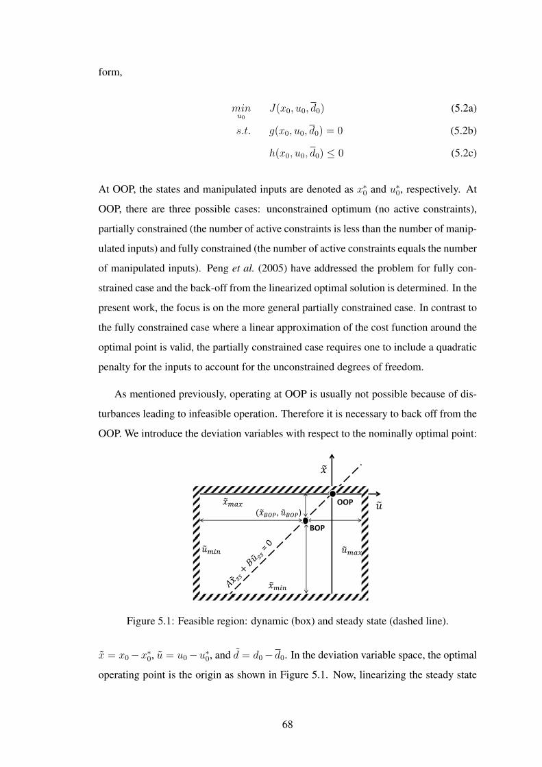
form,

minu0

J(x0, u0, d0) (5.2a)

s.t. g(x0, u0, d0) = 0 (5.2b)

h(x0, u0, d0) ≤ 0 (5.2c)

At OOP, the states and manipulated inputs are denoted as x∗0 and u∗0, respectively. At

OOP, there are three possible cases: unconstrained optimum (no active constraints),

partially constrained (the number of active constraints is less than the number of manip-

ulated inputs) and fully constrained (the number of active constraints equals the number

of manipulated inputs). Peng et al. (2005) have addressed the problem for fully con-

strained case and the back-off from the linearized optimal solution is determined. In the

present work, the focus is on the more general partially constrained case. In contrast to

the fully constrained case where a linear approximation of the cost function around the

optimal point is valid, the partially constrained case requires one to include a quadratic

penalty for the inputs to account for the unconstrained degrees of freedom.

As mentioned previously, operating at OOP is usually not possible because of dis-

turbances leading to infeasible operation. Therefore it is necessary to back off from the

OOP. We introduce the deviation variables with respect to the nominally optimal point:

𝑢 (𝑥 𝐵𝑂𝑃, 𝑢 𝐵𝑂𝑃)

𝑥

𝑢 𝑚𝑎𝑥 𝑢 𝑚𝑖𝑛

𝑥 𝑚𝑎𝑥

𝑥 𝑚𝑖𝑛

OOP

BOP

Figure 5.1: Feasible region: dynamic (box) and steady state (dashed line).

x = x0−x∗0, u = u0−u∗0, and d = d0− d0. In the deviation variable space, the optimal

operating point is the origin as shown in Figure 5.1. Now, linearizing the steady state

68

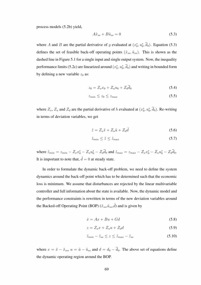
process models (5.2b) yield,

Axss +Buss = 0 (5.3)

where A and B are the partial derivative of g evaluated at (x∗0, u∗0, d0). Equation (5.3)

defines the set of feasible back-off operating points (xss, uss). This is shown as the

dashed line in Figure 5.1 for a single input and single output system. Now, the inequality

performance limits (5.2c) are linearized around (x∗0, u∗0, d0) and writing in bounded form

by defining a new variable z0 as:

z0 = Zxx0 + Zuu0 + Zdd0 (5.4)

zmin ≤ z0 ≤ zmax (5.5)

where Zx, Zu and Zd are the partial derivative of h evaluated at (x∗0, u∗0, d0). Re-writing

in terms of deviation variables, we get

z = Zxx+ Zuu+ Zdd (5.6)

zmin ≤ z ≤ zmax (5.7)

where zmin = zmin − Zxx∗0 − Zuu∗0 − Zdd0 and zmax = zmax − Zxx∗0 − Zuu∗0 − Zdd0.

It is important to note that, d = 0 at steady state.

In order to formulate the dynamic back-off problem, we need to define the system

dynamics around the back-off point which has to be determined such that the economic

loss is minimum. We assume that disturbances are rejected by the linear multivariable

controller and full information about the state is available. Now, the dynamic model and

the performance constraints is rewritten in terms of the new deviation variables around

the Backed-off Operating Point (BOP) (xss,uss,d) and is given by

x = Ax+Bu+Gd (5.8)

z = Zxx+ Zuu+ Zdd (5.9)

zmin − zss ≤ z ≤ zmax − zss (5.10)

where x = x − xss, u = u − uss and d = d0 − d0. The above set of equations define

the dynamic operating region around the BOP.

69

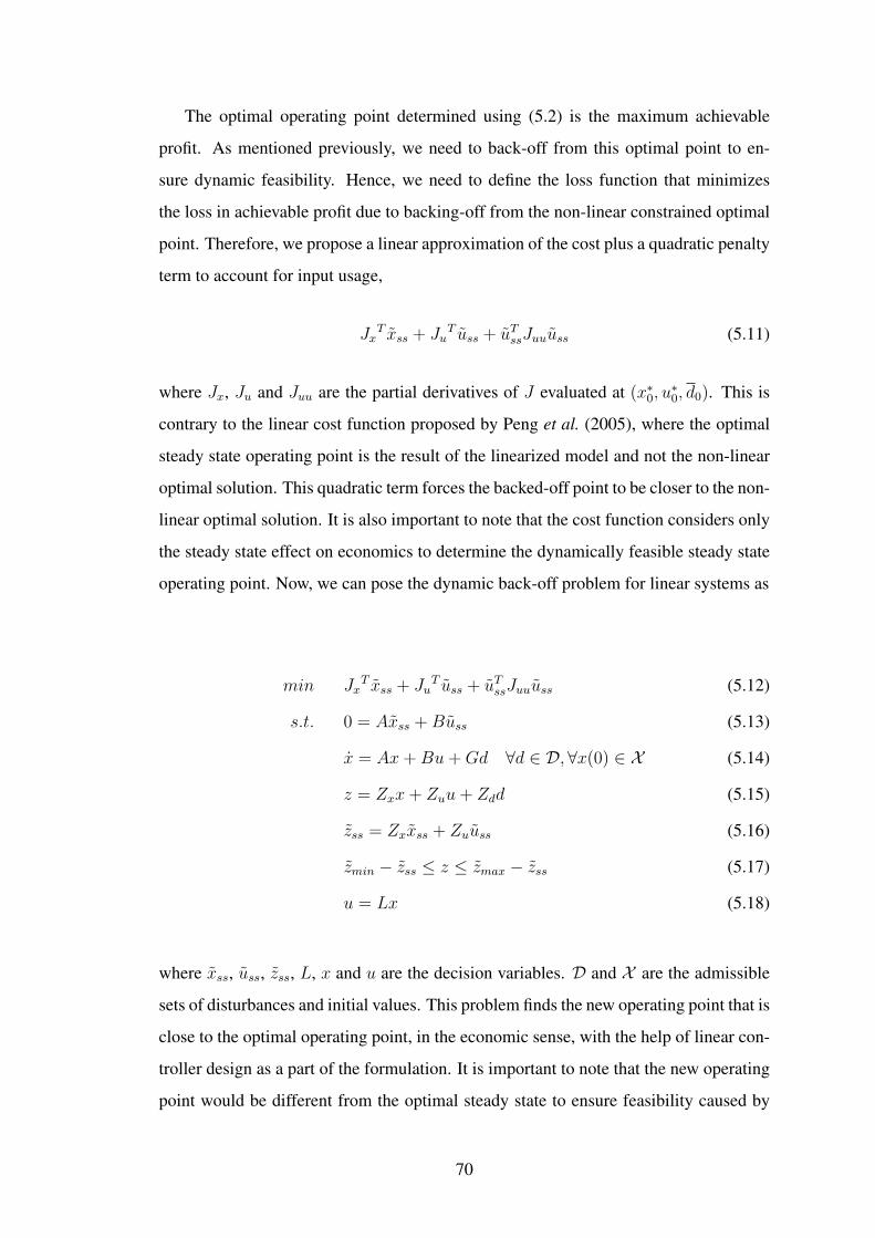
The optimal operating point determined using (5.2) is the maximum achievable

profit. As mentioned previously, we need to back-off from this optimal point to en-

sure dynamic feasibility. Hence, we need to define the loss function that minimizes

the loss in achievable profit due to backing-off from the non-linear constrained optimal

point. Therefore, we propose a linear approximation of the cost plus a quadratic penalty

term to account for input usage,

JxT xss + Ju

T uss + uTssJuuuss (5.11)

where Jx, Ju and Juu are the partial derivatives of J evaluated at (x∗0, u∗0, d0). This is

contrary to the linear cost function proposed by Peng et al. (2005), where the optimal

steady state operating point is the result of the linearized model and not the non-linear

optimal solution. This quadratic term forces the backed-off point to be closer to the non-

linear optimal solution. It is also important to note that the cost function considers only

the steady state effect on economics to determine the dynamically feasible steady state

operating point. Now, we can pose the dynamic back-off problem for linear systems as

min JxT xss + Ju

T uss + uTssJuuuss (5.12)

s.t. 0 = Axss +Buss (5.13)

x = Ax+Bu+Gd ∀d ∈ D,∀x(0) ∈ X (5.14)

z = Zxx+ Zuu+ Zdd (5.15)

zss = Zxxss + Zuuss (5.16)

zmin − zss ≤ z ≤ zmax − zss (5.17)

u = Lx (5.18)

where xss, uss, zss, L, x and u are the decision variables. D and X are the admissible

sets of disturbances and initial values. This problem finds the new operating point that is

close to the optimal operating point, in the economic sense, with the help of linear con-

troller design as a part of the formulation. It is important to note that the new operating

point would be different from the optimal steady state to ensure feasibility caused by

70

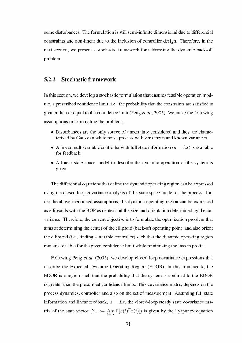
some disturbances. The formulation is still semi-infinite dimensional due to differential

constraints and non-linear due to the inclusion of controller design. Therefore, in the

next section, we present a stochastic framework for addressing the dynamic back-off

problem.

5.2.2 Stochastic framework

In this section, we develop a stochastic formulation that ensures feasible operation mod-

ulo, a prescribed confidence limit, i.e., the probability that the constraints are satisfied is

greater than or equal to the confidence limit (Peng et al., 2005). We make the following

assumptions in formulating the problem:

• Disturbances are the only source of uncertainty considered and they are charac-terized by Gaussian white noise process with zero mean and known variances.

• A linear multi-variable controller with full state information (u = Lx) is availablefor feedback.

• A linear state space model to describe the dynamic operation of the system isgiven.

The differential equations that define the dynamic operating region can be expressed

using the closed loop covariance analysis of the state space model of the process. Un-

der the above-mentioned assumptions, the dynamic operating region can be expressed

as ellipsoids with the BOP as center and the size and orientation determined by the co-

variance. Therefore, the current objective is to formulate the optimization problem that

aims at determining the center of the ellipsoid (back-off operating point) and also orient

the ellipsoid (i.e., finding a suitable controller) such that the dynamic operating region

remains feasible for the given confidence limit while minimizing the loss in profit.

Following Peng et al. (2005), we develop closed loop covariance expressions that

describe the Expected Dynamic Operating Region (EDOR). In this framework, the

EDOR is a region such that the probability that the system is confined to the EDOR

is greater than the prescribed confidence limits. This covariance matrix depends on the

process dynamics, controller and also on the set of measurement. Assuming full state

information and linear feedback, u = Lx, the closed-loop steady state covariance ma-

trix of the state vector (Σx := limt→∞

E[x(t)Tx(t)]) is given by the Lyapunov equation

71

(A+BL)Σx + Σx(A+BL)T +GΣdGT = 0 (5.19)

where Σx is the symmetric positive semi-definite solution to the Lyapunov equation.

Correspondingly, the covariance of the output signal z is given by

Σz = (Zx + ZuL)Σx(Zx + ZuL)T + ZdΣdZdT (5.20)

Given the center, zss, and the covariance Σz = P 2, the ellipsoidal EDOR is expressed

as

E = {zss + αPz | ‖z‖2 ≤ 1} (5.21)

where P is the positive square root of Σz and α depends on the confidence limit (e.g.,

for a confidence limit of 95%, α = 2). It is important to note that z = zss+αPz. There-

fore, we describe the dynamic feasibility as finding the ellipsoid within the performance

bounds which is given by

E = {(zmin ≤ zss + αPz ≤ zmax) | ‖z‖2 ≤ 1} (5.22)

This representation ensures that the whole ellipsoid should lie within the performance

bounds defined by (5.7). These bounds can be written as hTi z + ti ≤ 0; i = 1, . . . ,m

where hi’s, ti’s are the respective rows and elements of the matrix H = [I;−I] and

vector t = [zmax;−zmin]. Thus, the problem can be restated as finding the center of

the ellipsoid close to the optimal operating point such that the ellipsoid is contained

within performance bounds. Thus, we write the Economic Backed-off Operating Point

72

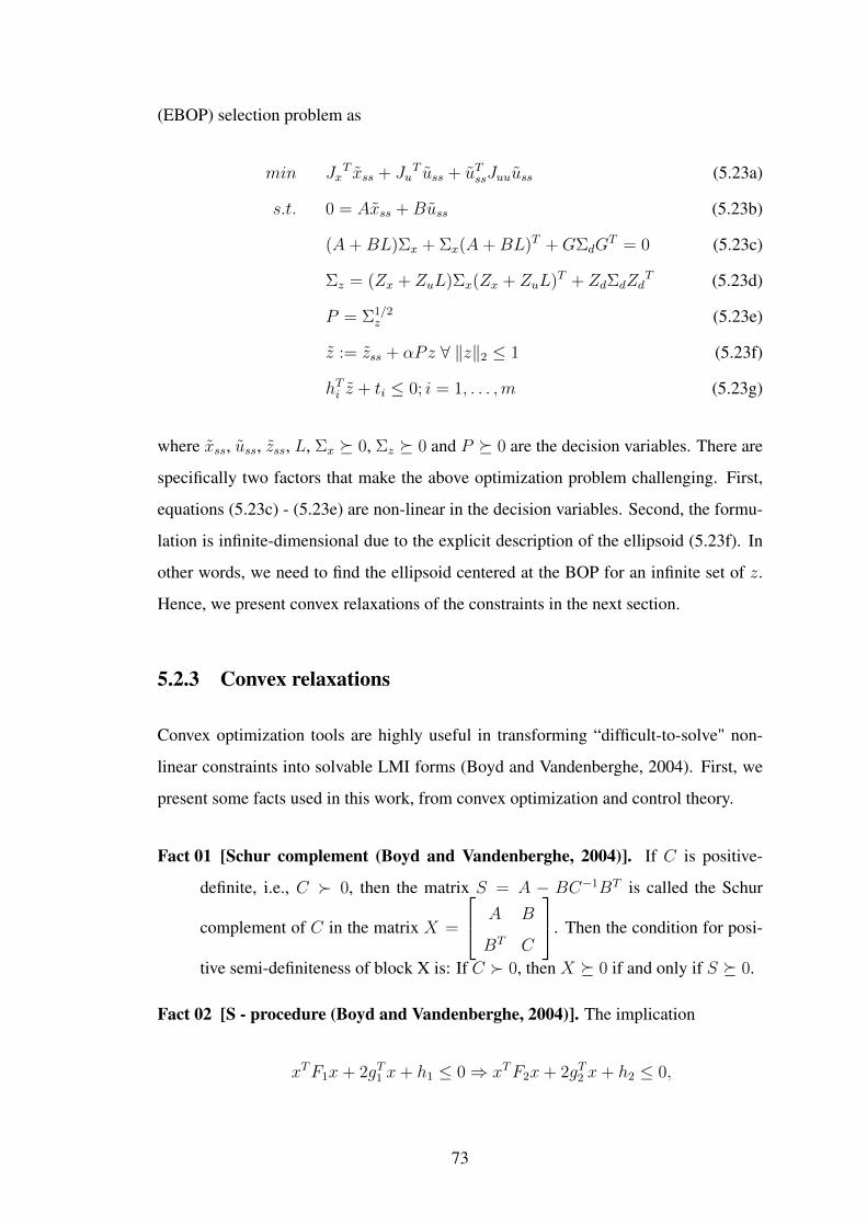
(EBOP) selection problem as

min JxT xss + Ju

T uss + uTssJuuuss (5.23a)

s.t. 0 = Axss +Buss (5.23b)

(A+BL)Σx + Σx(A+BL)T +GΣdGT = 0 (5.23c)

Σz = (Zx + ZuL)Σx(Zx + ZuL)T + ZdΣdZdT (5.23d)

P = Σ1/2z (5.23e)

z := zss + αPz ∀ ‖z‖2 ≤ 1 (5.23f)

hTi z + ti ≤ 0; i = 1, . . . ,m (5.23g)

where xss, uss, zss, L, Σx � 0, Σz � 0 and P � 0 are the decision variables. There are

specifically two factors that make the above optimization problem challenging. First,

equations (5.23c) - (5.23e) are non-linear in the decision variables. Second, the formu-

lation is infinite-dimensional due to the explicit description of the ellipsoid (5.23f). In

other words, we need to find the ellipsoid centered at the BOP for an infinite set of z.

Hence, we present convex relaxations of the constraints in the next section.

5.2.3 Convex relaxations

Convex optimization tools are highly useful in transforming “difficult-to-solve" non-

linear constraints into solvable LMI forms (Boyd and Vandenberghe, 2004). First, we

present some facts used in this work, from convex optimization and control theory.

Fact 01 [Schur complement (Boyd and Vandenberghe, 2004)]. If C is positive-

definite, i.e., C � 0, then the matrix S = A − BC−1BT is called the Schur

complement of C in the matrix X =

A B

BT C

. Then the condition for posi-

tive semi-definiteness of block X is: If C � 0, then X � 0 if and only if S � 0.

Fact 02 [S - procedure (Boyd and Vandenberghe, 2004)]. The implication

xTF1x+ 2gT1 x+ h1 ≤ 0⇒ xTF2x+ 2gT2 x+ h2 ≤ 0,

73

where Fi ∈ Sn,gi ∈ Rn,hi ∈ R, holds if and only if there exists a τ such that

τ ≥ 0;

F2 g2

gT2 h2

� τ

F1 g1

gT1 h1

,provided there exists a point x with xTF1x+ 2gT1 x+ h1 < 0.

Theorem 5.2.1 (Peng et al., 2005) ∃ stabilizing L, Σx � 0 s.t. (A+BL)Σx + Σx(A+

BL)T +GΣdGT = 0 and Σz = (Zx + ZuL)Σx(Zx + ZuL)T + ZdΣdZd

T if and only if

∃ Y ,X � 0 and Z � 0 s.t.

(AX +BY ) + (AX +BY )T +GΣdGT ≺ 0, Z − ZdΣdZd

T ZxX + ZuY

(ZxX + ZuY )T X

� 0.

For proof of the above theorem, the reader is referred to Chmielewski and co-workers

(Peng et al., 2005).

Corollary 5.2.2 The controller gain is recovered as L = Y X−1 and the covariance

matrix of the states is Σx = X .

Theorem 5.2.3 (Boyd and Vandenberghe, 2004) Equations (5.23f) - (5.23g) can be

expressed as a set of second order cone constraints of the form ‖αPhi‖2 +hTi zss+ ti ≤

0.

Proof . Recall that the feasibility condition, hTi z + ti ≤ 0 ∀αPz + zss| ‖z‖2 ≤ 1. This

can be rewritten as

sup‖z‖2≤1

hTi (αPz + zss) + ti ≤ 0, i = 1, . . . ,m

⇐⇒ sup‖z‖2≤1

(hTi αPz) + hTi zss + ti ≤ 0, i = 1, . . . ,m

⇐⇒ ‖αPhi‖2 + hTi zss + ti ≤ 0, i = 1, . . . ,m

Let us consider the covariance constraint (5.23d) of the output z

Σz = (Zx + ZuL)ΣxΣ−1x Σx(Zx + ZuL)T + ZdΣdZd

T (5.24)

74

Taking Σx within brackets, we get

Σz = (ZxΣx + ZuLΣx)Σ−1x (ZxΣx + ZuLΣx)

T + ZdΣdZdT (5.25)

This form allows one to write it as an LMI using change of variables and Schur com-

plement (see Fact 01). Next, let us consider the ellipsoidal constraint (5.23f) and the

output bounds defined by the polytopic constraint (5.23g). As mentioned previously,

these two constraints make the EBOP selection problem as an infinite dimensional one.

However, we can represent them using finite number of second order cone constraints

using Theorem 5.2.3

‖αPhi‖2 + hTi zss + ti ≤ 0, i = 1, . . . ,m (5.26)

Now the EBOP selection problem is reformulated in terms of LMI constraints as :

min JxT xss + Ju

T uss + uTssJuuuss (5.27a)

s.t. 0 = Axss +Buss (5.27b)

zss = Zxxss + Zuuss (5.27c)

(AX +BY ) + (AX +BY )T +GΣdGT ≺ 0 (5.27d) Z − ZdΣdZd

T ZxX + ZuY

(ZxX + ZuY )T X

� 0 (5.27e)

P = Z1/2 (5.27f)

‖αPhi‖2 + hTi zss + ti ≤ 0, i = 1, . . . , 2nz (5.27g)

where xss, uss, zss, Y , X � 0, Z � 0 and P � 0 are the decision variables. The

objective function and all the constraints in the above formulation (5.27) except (5.27f)

are convex. Thus, the formulated minimum back off operating point selection problem

is a non-linear and non-convex program. However, this problem is solved using the

solution methodology developed in Section 5.3.

Remarks

1. The formulation presented in Peng et al. (2005) differs from our formulationin many ways: (1) there is no explicit ellipsoidal constraints, (2) the dynamic

75

feasibility of the ellipsoid is ensured by the reverse convex constraints and, (3) abranch and bound type of algorithm was proposed.

2. Note that this cost function considers only the steady state effect on economics.Since the disturbances are assumed to be Gaussian and zero mean, this impliesthat the cost accounts only for the nominal steady state value of disturbances.

3. The linear terms in the cost function could be interpreted as the sum of the productof back-off variables and their Lagrange multipliers.

4. By direct comparison of (5.27g) with the robust LP with random constraints(Boyd and Vandenberghe, 2004),

Φ−1(η)‖Phi‖2 + hTi zss + ti ≤ 0 (5.28)

we can choose the parameter α using the inverse of the cumulative distributionfunction Φ−1(η) where η denotes the probability level of a particular constraintbeing satisfied.

5. The term ‖αPhi‖2 denotes the amount of required back-off. Hence, given thecontroller design, we can directly compute the back-off from the covariance esti-mates.

6. An equivalent LMI representation of the second order cone constraints (5.27g) isgiven by S-procedure (see Fact 02),[

−τi − hiT zss − ti α2hiTP

(α2hiTP )T τiI

]� 0; τi > 0; i = 1 · · · 2nz (5.29)

7. Hard and soft constraints could be handled within the proposed formulation byselecting different values α for each of the constraints. Higher value of α ischosen for a hard constraint which signifies that probability of violating that con-straint should be less. On the other hand, lower values of α are chosen for softconstraints to achieve the appropriate tolerance level.

5.3 Solution methodology

The main challenge in obtaining solution to the proposed formulation is the non-linearity

in Z. In our formulation, the objective was to orient the ellipsoid (i.e., controller gain,

L) such that the center of the ellipsoid is close to optimal operating point (i.e., EBOP,

zss). In this section, we present a solution technique to solve the proposed formula-

tion using the geometrical inference of the solution space. In this regard, we develop a

two-stage iterative procedure where a convex problem is solved in each stage.

76

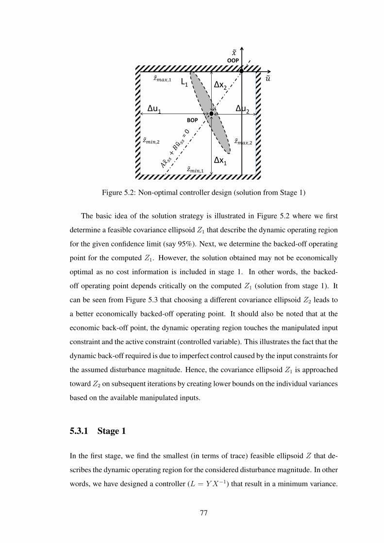
Δu2 Δu1

Δx1

Δx2

OOP

BOP

L1

𝑥

𝑢

𝑧 𝑚𝑎𝑥,2 𝑧 𝑚𝑖𝑛,2

𝑧 𝑚𝑎𝑥,1

𝑧 𝑚𝑖𝑛,1

Figure 5.2: Non-optimal controller design (solution from Stage 1)

The basic idea of the solution strategy is illustrated in Figure 5.2 where we first

determine a feasible covariance ellipsoid Z1 that describe the dynamic operating region

for the given confidence limit (say 95%). Next, we determine the backed-off operating

point for the computed Z1. However, the solution obtained may not be economically

optimal as no cost information is included in stage 1. In other words, the backed-

off operating point depends critically on the computed Z1 (solution from stage 1). It

can be seen from Figure 5.3 that choosing a different covariance ellipsoid Z2 leads to

a better economically backed-off operating point. It should also be noted that at the

economic back-off point, the dynamic operating region touches the manipulated input

constraint and the active constraint (controlled variable). This illustrates the fact that the

dynamic back-off required is due to imperfect control caused by the input constraints for

the assumed disturbance magnitude. Hence, the covariance ellipsoid Z1 is approached

towardZ2 on subsequent iterations by creating lower bounds on the individual variances

based on the available manipulated inputs.

5.3.1 Stage 1

In the first stage, we find the smallest (in terms of trace) feasible ellipsoid Z that de-

scribes the dynamic operating region for the considered disturbance magnitude. In other

words, we have designed a controller (L = Y X−1) that result in a minimum variance.

77

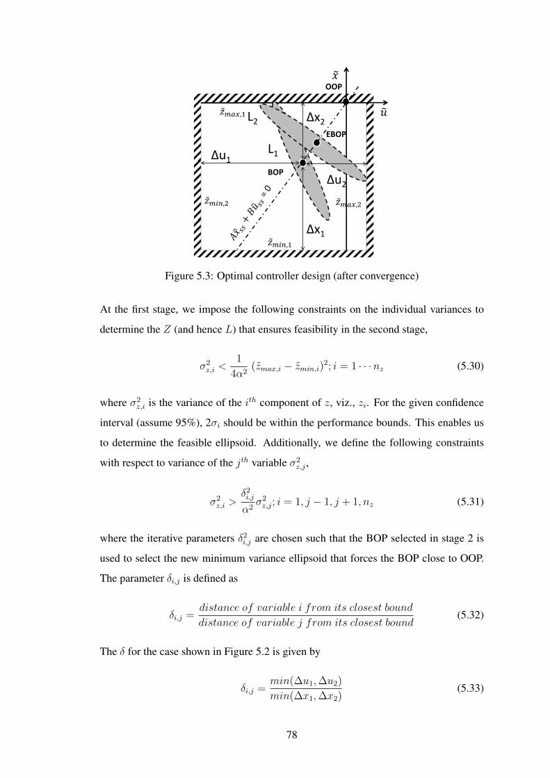
Δu2

Δu1

Δx1

Δx2

OOP

BOP

L1

L2 EBOP

𝑥

𝑢

𝑧 𝑚𝑎𝑥,2 𝑧 𝑚𝑖𝑛,2

𝑧 𝑚𝑎𝑥,1

𝑧 𝑚𝑖𝑛,1

Figure 5.3: Optimal controller design (after convergence)

At the first stage, we impose the following constraints on the individual variances to

determine the Z (and hence L) that ensures feasibility in the second stage,

σ2z,i <

1

4α2(zmax,i − zmin,i)2; i = 1 · · ·nz (5.30)

where σ2z,i is the variance of the ith component of z, viz., zi. For the given confidence

interval (assume 95%), 2σi should be within the performance bounds. This enables us

to determine the feasible ellipsoid. Additionally, we define the following constraints

with respect to variance of the jth variable σ2z,j ,

σ2z,i >

δ2i,j

α2σ2z,j; i = 1, j − 1, j + 1, nz (5.31)

where the iterative parameters δ2i,j are chosen such that the BOP selected in stage 2 is

used to select the new minimum variance ellipsoid that forces the BOP close to OOP.

The parameter δi,j is defined as

δi,j =distance of variable i from its closest bound

distance of variable j from its closest bound(5.32)

The δ for the case shown in Figure 5.2 is given by

δi,j =min(∆u1,∆u2)

min(∆x1,∆x2)(5.33)

78

Physically, the solution tries to exploit the available manipulated input space to be

utilized to find the economic back-off point and the optimal multi-variable controller.

Hence, we solve the following problem to find the dynamic operating region:

minX�0,Z�0,Y

Tr(Z) (5.34a)

s.t. (AX +BY ) + (AX +BY )T +GΣdGT ≺ 0 (5.34b) Z − ZdΣdZd

T ZxX + ZuY

(ZxX + ZuY )T X

� 0 (5.34c)

σ2z,i <

1

4α2(zmax,i − zmin,i)2; i = 1 · · ·nz (5.34d)

σ2z,i >

δ2i,j

α2σ2z,j; i = 1, j − 1, j + 1, nz (5.34e)

The solution of stage 1 results in a feasible covariance ellipsoid Z1. The upper bound

on the individual variances ensure that Z1 is feasible in the second stage. If the solution

from stage 1 is infeasible, then the solution to the original problem is infeasible. The

parameter δ is used to create lower bounds on the individual variances such that the

economically optimal ellipsoid is approached on subsequent iterations. The parameter

δ is initialized to zero during the start of the algorithm which defines that the individual

variances should be non-negative. Hence, on solving the first stage problem, we obtain

Z and letting P = Z1/2, a second optimization problem is solved to obtain the back-off

point. This would yield an approximation to the economic back-off point.

5.3.2 Stage 2

minxss,uss,zss

JxT xss + Ju

T uss + uTssJuuuss (5.35a)

s.t. Axss +Buss = 0 (5.35b)

zss = Zxxss + Zuuss (5.35c)

‖αPhi‖2 + hTi zss + ti ≤ 0, i = 1, . . . , 2nz (5.35d)

In the second stage, we determine a backed-off operating point (zss) that is close to the

optimal point for the predetermined ellipsoid (solution from the first stage). However,

the proximity to the economically optimal point depends on the orientation of the co-

79

Table 5.1: Algorithm for selecting economic back-off operating point

1 Initialize the parameter δi,j = 0.2 Find Z by solving the Stage 1 convex problem (5.34). If no feasible Z can be

found, exit.3 Compute P = Z1/2. Find the BOP (zss) by solving the Stage 2 convex problem

(5.35).4 Terminate on convergence. Otherwise, update δi,j using (5.32) and proceed to

Step 2.

variance ellipsoid. As we have written the inequalities as box constraints, the surface

of the ellipsoid should touch the box at optimality. Hence, we need to re-orient the

ellipsoid such that dynamic operating region touches the box constraint. This is ac-

complished by creating lower bounds for the individual variances using the parameter

δ. The δ’s are updated based on the newly found backed-off point. This information

is used to recompute Z (and hence L) in the first stage. This process is iterated until

convergence. It should be noted that P is not a decision variable since Z is known

from the first stage. Now, it can be easily recognized that both stages contains only

convex constraints, which could be easily solved using CVX, a package for specifying

and solving convex programs (Grant and Boyd, 2011). Initializing δi,j to zero and given

two successive iterates, ziter−1ss and ziterss this process is iterated until the convergence

criteria ‖ziterss − ziter-1ss ‖2 ≤ ε is satisfied where ε being the prescribed tolerance limit.

The solution algorithm is presented in Table 5.1.

5.4 Illustrations

5.4.1 Mass spring damper system

The purpose of this example is to illustrate the proposed backed-off operating point

selection algorithm in a single-input two-output system.

Description. Consider the mass-spring-damper system depicted in Figure 5.4. Let r

denote the mass position, v the velocity, g the gravitational force, f the manipulated

input force, and w a disturbance force. The system dynamics are described by linear

80

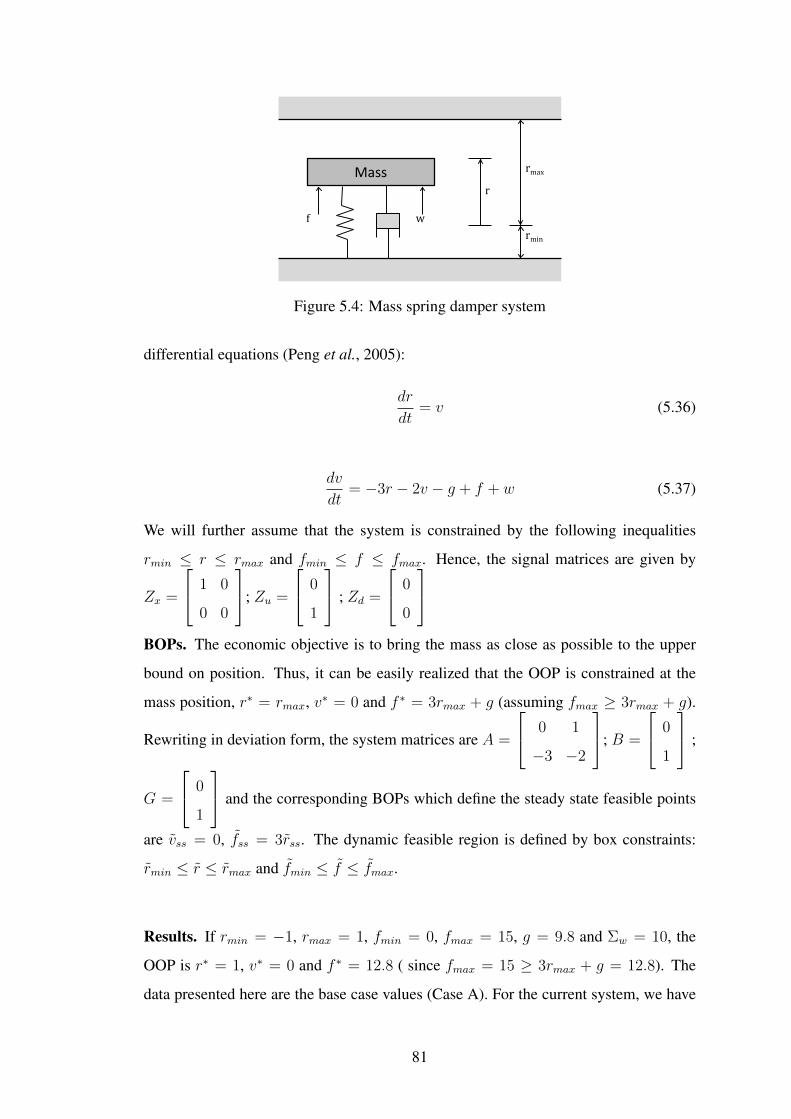
Mass

f w

r

rmax

rmin

Figure 5.4: Mass spring damper system

differential equations (Peng et al., 2005):

dr

dt= v (5.36)

dv

dt= −3r − 2v − g + f + w (5.37)

We will further assume that the system is constrained by the following inequalities

rmin ≤ r ≤ rmax and fmin ≤ f ≤ fmax. Hence, the signal matrices are given by

Zx =

1 0

0 0

; Zu =

0

1

; Zd =

0

0

BOPs. The economic objective is to bring the mass as close as possible to the upper

bound on position. Thus, it can be easily realized that the OOP is constrained at the

mass position, r∗ = rmax, v∗ = 0 and f ∗ = 3rmax + g (assuming fmax ≥ 3rmax + g).

Rewriting in deviation form, the system matrices are A =

0 1

−3 −2

; B =

0

1

;

G =

0

1

and the corresponding BOPs which define the steady state feasible points

are vss = 0, fss = 3rss. The dynamic feasible region is defined by box constraints:

rmin ≤ r ≤ rmax and fmin ≤ f ≤ fmax.

Results. If rmin = −1, rmax = 1, fmin = 0, fmax = 15, g = 9.8 and Σw = 10, the

OOP is r∗ = 1, v∗ = 0 and f ∗ = 12.8 ( since fmax = 15 ≥ 3rmax + g = 12.8). The

data presented here are the base case values (Case A). For the current system, we have

81

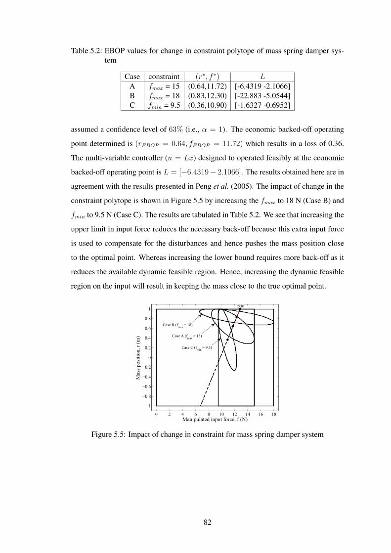
Table 5.2: EBOP values for change in constraint polytope of mass spring damper sys-tem

Case constraint (r∗, f ∗) LA fmax = 15 (0.64,11.72) [-6.4319 -2.1066]B fmax = 18 (0.83,12.30) [-22.883 -5.0544]C fmin = 9.5 (0.36,10.90) [-1.6327 -0.6952]

assumed a confidence level of 63% (i.e., α = 1). The economic backed-off operating

point determined is (rEBOP = 0.64, fEBOP = 11.72) which results in a loss of 0.36.

The multi-variable controller (u = Lx) designed to operated feasibly at the economic

backed-off operating point is L = [−6.4319− 2.1066]. The results obtained here are in

agreement with the results presented in Peng et al. (2005). The impact of change in the

constraint polytope is shown in Figure 5.5 by increasing the fmax to 18 N (Case B) and

fmin to 9.5 N (Case C). The results are tabulated in Table 5.2. We see that increasing the

upper limit in input force reduces the necessary back-off because this extra input force

is used to compensate for the disturbances and hence pushes the mass position close

to the optimal point. Whereas increasing the lower bound requires more back-off as it

reduces the available dynamic feasible region. Hence, increasing the dynamic feasible

region on the input will result in keeping the mass close to the true optimal point.

0 2 4 6 8 10 12 14 16 18

−1

−0.8

−0.6

−0.4

−0.2

0

0.2

0.4

0.6

0.8

1

Manipulated input force, f (N)

Mas

s pos

ition

, r (m

)

Case A (fmax

= 15)

Case C (fmin

= 9.5)

Case B (fmax

= 18)

OOP

Figure 5.5: Impact of change in constraint for mass spring damper system

82

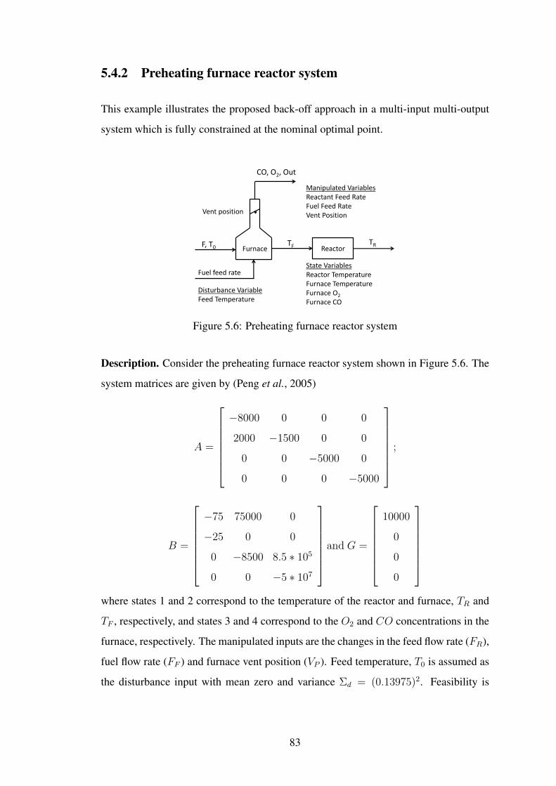
5.4.2 Preheating furnace reactor system

This example illustrates the proposed back-off approach in a multi-input multi-output

system which is fully constrained at the nominal optimal point.

Reactor Furnace

CO, O2, Out

Fuel feed rate

F, T0 TF TR

Vent position

Manipulated Variables Reactant Feed Rate Fuel Feed Rate Vent Position

State Variables Reactor Temperature Furnace Temperature Furnace O2

Furnace CO

Disturbance Variable Feed Temperature

Figure 5.6: Preheating furnace reactor system

Description. Consider the preheating furnace reactor system shown in Figure 5.6. The

system matrices are given by (Peng et al., 2005)

A =

−8000 0 0 0

2000 −1500 0 0

0 0 −5000 0

0 0 0 −5000

;

B =

−75 75000 0

−25 0 0

0 −8500 8.5 ∗ 105

0 0 −5 ∗ 107

and G =

10000

0

0

0

where states 1 and 2 correspond to the temperature of the reactor and furnace, TR and

TF , respectively, and states 3 and 4 correspond to the O2 and CO concentrations in the

furnace, respectively. The manipulated inputs are the changes in the feed flow rate (FR),

fuel flow rate (FF ) and furnace vent position (VP ). Feed temperature, T0 is assumed as

the disturbance input with mean zero and variance Σd = (0.13975)2. Feasibility is

83

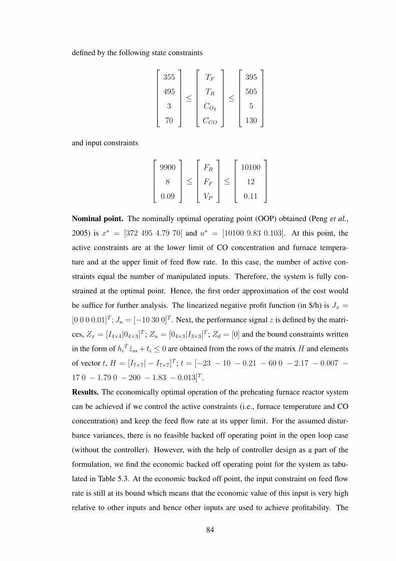
defined by the following state constraints355

495

3

70

≤

TF

TR

CO2

CCO

≤

395

505

5

130

and input constraints

9900

8

0.09

≤FR

FF

VP

≤

10100

12

0.11

Nominal point. The nominally optimal operating point (OOP) obtained (Peng et al.,

2005) is x∗ = [372 495 4.79 70] and u∗ = [10100 9.83 0.103]. At this point, the

active constraints are at the lower limit of CO concentration and furnace tempera-

ture and at the upper limit of feed flow rate. In this case, the number of active con-

straints equal the number of manipulated inputs. Therefore, the system is fully con-

strained at the optimal point. Hence, the first order approximation of the cost would

be suffice for further analysis. The linearized negative profit function (in $/h) is Jx =

[0 0 0 0.01]T ; Ju = [−10 30 0]T . Next, the performance signal z is defined by the matri-

ces, Zx = [I4×4|04×3]T ; Zu = [04×3|I3×3]T ; Zd = [0] and the bound constraints written

in the form of hiT zss + ti ≤ 0 are obtained from the rows of the matrix H and elements

of vector t, H = [I7×7| − I7×7]T ; t = [−23 − 10 − 0.21 − 60 0 − 2.17 − 0.007 −

17 0 − 1.79 0 − 200 − 1.83 − 0.013]T .

Results. The economically optimal operation of the preheating furnace reactor system

can be achieved if we control the active constraints (i.e., furnace temperature and CO

concentration) and keep the feed flow rate at its upper limit. For the assumed distur-

bance variances, there is no feasible backed off operating point in the open loop case

(without the controller). However, with the help of controller design as a part of the

formulation, we find the economic backed off operating point for the system as tabu-

lated in Table 5.3. At the economic backed off point, the input constraint on feed flow

rate is still at its bound which means that the economic value of this input is very high

relative to other inputs and hence other inputs are used to achieve profitability. The

84

Table 5.3: Nominal values and EBOP solution of the preheater furnace reactor system

Variables Description Units Nominal values EBOP (closed loop)States (x)

TR reactor temperature ◦C 495 496.45TF furnace temperature ◦C 372 373.09CO2 O2 concentration ppm 4.79 4.2517CCO CO concentration ppm 70 90.083

Inputs (u)FR feed flow rate bbl/day 10100 10100FF fuel flow rate bbl/day 9.83 9.9458VP furnace vent position % 0.103 0.10099

dynamic operating region along with the economic back-off point for the assumed con-

fidence level is shown in Figures 5.7 - 5.12. We can see that, in order to ensure dynamic

feasibility, the furnace temperature and CO concentration are backed-off from the ac-

tive constraints whereas feed flow rate requires no back-off. However, increasing the

disturbance magnitude may demand the feed flow rate to be backed-off. The optimal

multivariable controller gain L designed using our approach is given by

L =

0.001 0.008 0.010 0.000

−0.538 −4.038 5.608 0.099

−0.001 −0.013 −33.498 1.249

It is important to note from the first row of the L matrix that the feed flow rate is hardly

adjusted under dynamic conditions. In other words, the feed flow rate should be kept at

its limiting value to achieve optimality. Therefore, other inputs (fuel flow rate and vent

position) are manipulated to ensure feasible operation under dynamic conditions. The

lost profit for operating the system at the economic backed-off operating point is $3.93

per day.

5.4.3 Evaporation process

In this example, we illustrate the backed-off operating point selection problem in a

partially constrained system, that is, when there exists some unconstrained degrees of

freedom at the nominal optimal point. Further, the economic impact of controller de-

sign is addressed.

85

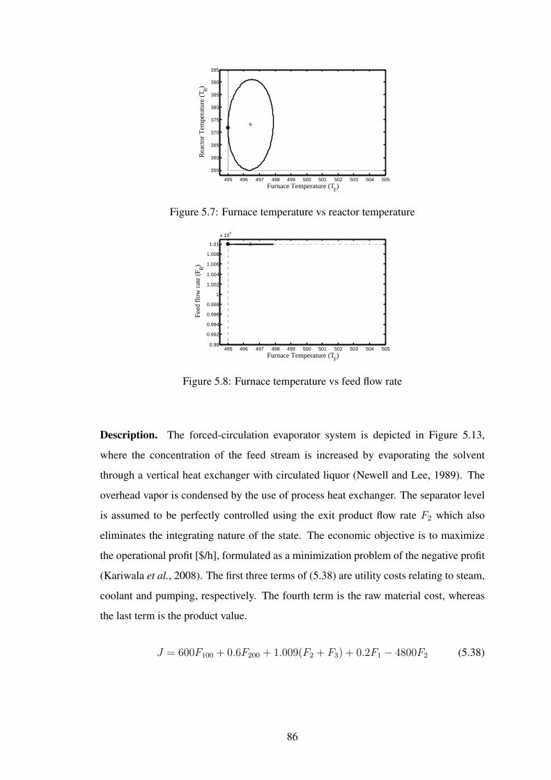
495 496 497 498 499 500 501 502 503 504 505

355

360

365

370

375

380

385

390

395

Furnace Temperature (TF)

Rea

ctor

Tem

pera

ture

(T R

)

Figure 5.7: Furnace temperature vs reactor temperature

495 496 497 498 499 500 501 502 503 504 5050.99

0.992

0.994

0.996

0.998

1

1.002

1.004

1.006

1.008

1.01

x 104

Furnace Temperature (TF)

Feed

flo

w r

ate

(FR)

Figure 5.8: Furnace temperature vs feed flow rate

Description. The forced-circulation evaporator system is depicted in Figure 5.13,

where the concentration of the feed stream is increased by evaporating the solvent

through a vertical heat exchanger with circulated liquor (Newell and Lee, 1989). The

overhead vapor is condensed by the use of process heat exchanger. The separator level

is assumed to be perfectly controlled using the exit product flow rate F2 which also

eliminates the integrating nature of the state. The economic objective is to maximize

the operational profit [$/h], formulated as a minimization problem of the negative profit

(Kariwala et al., 2008). The first three terms of (5.38) are utility costs relating to steam,

coolant and pumping, respectively. The fourth term is the raw material cost, whereas

the last term is the product value.

J = 600F100 + 0.6F200 + 1.009(F2 + F3) + 0.2F1 − 4800F2 (5.38)

86

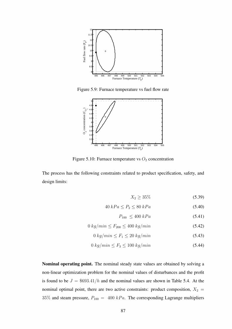
495 496 497 498 499 500 501 502 503 504 505

8

8.5

9

9.5

10

10.5

11

11.5

12

Furnace Temperature (TF)

Fuel

flo

w r

ate

(FF)

Figure 5.9: Furnace temperature vs fuel flow rate

495 496 497 498 499 500 501 502 503 504 5053

3.2

3.4

3.6

3.8

4

4.2

4.4

4.6

4.8

5

Furnace Temperature (TF)

O2 c

once

ntra

tion

(CO

2)

Figure 5.10: Furnace temperature vs O2 concentration

The process has the following constraints related to product specification, safety, and

design limits:

X2 ≥ 35% (5.39)

40 kPa ≤ P2 ≤ 80 kPa (5.40)

P100 ≤ 400 kPa (5.41)

0 kg/min ≤ F200 ≤ 400 kg/min (5.42)

0 kg/min ≤ F1 ≤ 20 kg/min (5.43)

0 kg/min ≤ F3 ≤ 100 kg/min (5.44)

Nominal operating point. The nominal steady state values are obtained by solving a

non-linear optimization problem for the nominal values of disturbances and the profit

is found to be J = $693.41/h and the nominal values are shown in Table 5.4. At the

nominal optimal point, there are two active constraints: product composition, X2 =

35% and steam pressure, P100 = 400 kPa. The corresponding Lagrange multipliers

87

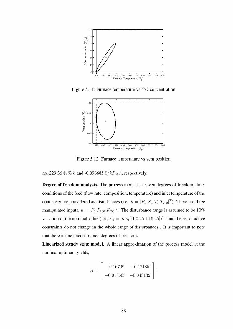
495 496 497 498 499 500 501 502 503 504 505

70

80

90

100

110

120

130

Furnace Temperature (TF)

CO

con

cent

ratio

n (C

CO

)

Figure 5.11: Furnace temperature vs CO concentration

495 496 497 498 499 500 501 502 503 504 5050.09

0.095

0.1

0.105

0.11

Furnace Temperature (TF)

Ven

t pos

ition

(V

P)

Figure 5.12: Furnace temperature vs vent position

are 229.36 $/% h and -0.096685 $/kPa h, respectively.

Degree of freedom analysis. The process model has seven degrees of freedom. Inlet

conditions of the feed (flow rate, composition, temperature) and inlet temperature of the

condenser are considered as disturbances (i.e., d = [F1 X1 T1 T200]T ). There are three

manipulated inputs, u = [F3 P100 F200]T . The disturbance range is assumed to be 10%

variation of the nominal value (i.e., Σd = diag([1 0.25 16 6.25])2 ) and the set of active

constraints do not change in the whole range of disturbances . It is important to note

that there is one unconstrained degrees of freedom.

Linearized steady state model. A linear approximation of the process model at the

nominal optimum yields,

A =

−0.16709 −0.17185

−0.013665 −0.043132

;

88

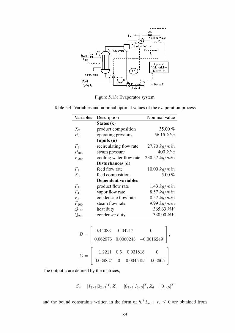
Figure 5.13: Evaporator system

Table 5.4: Variables and nominal optimal values of the evaporation process

Variables Description Nominal valueStates (x)

X2 product composition 35.00 %P2 operating pressure 56.15 kPa

Inputs (u)F3 recirculating flow rate 27.70 kg/minP100 steam pressure 400 kPaF200 cooling water flow rate 230.57 kg/min

Disturbances (d)F1 feed flow rate 10.00 kg/minX1 feed composition 5.00 %

Dependent variablesF2 product flow rate 1.43 kg/minF4 vapor flow rate 8.57 kg/minF5 condensate flow rate 8.57 kg/minF100 steam flow rate 9.99 kg/minQ100 heat duty 365.63 kWQ200 condenser duty 330.00 kW

B =

0.44083 0.04217 0

0.062976 0.0060243 −0.0016249

;

G =

−1.2211 0.5 0.031818 0

0.039837 0 0.0045455 0.03665

The output z are defined by the matrices,

Zx = [I2×2|02×3]T ;Zu = [03×2|I3×3]T ;Zd = [04×5]T

and the bound constraints written in the form of hiT zss + ti ≤ 0 are obtained from

89

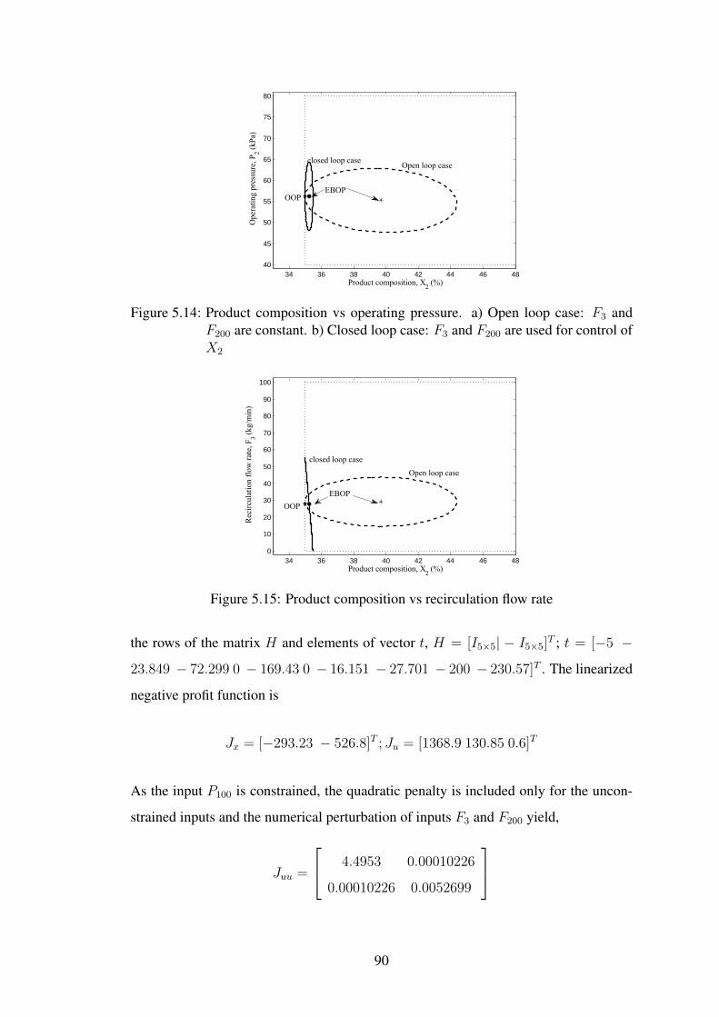
34 36 38 40 42 44 46 4840

45

50

55

60

65

70

75

80

Product composition, X2 (%)

Ope

ratin

g pr

essu

re, P

2 (kPa

)

OOP

Open loop case

EBOP

closed loop case

Figure 5.14: Product composition vs operating pressure. a) Open loop case: F3 andF200 are constant. b) Closed loop case: F3 and F200 are used for control ofX2

34 36 38 40 42 44 46 480

10

20

30

40

50

60

70

80

90

100

Product composition, X2 (%)

Rec

ircul

atio

n flo

w ra

te, F

3 (kg/

min

)

OOPEBOP

Open loop case

closed loop case

Figure 5.15: Product composition vs recirculation flow rate

the rows of the matrix H and elements of vector t, H = [I5×5| − I5×5]T ; t = [−5 −

23.849 − 72.299 0 − 169.43 0 − 16.151 − 27.701 − 200 − 230.57]T . The linearized

negative profit function is

Jx = [−293.23 − 526.8]T ; Ju = [1368.9 130.85 0.6]T

As the input P100 is constrained, the quadratic penalty is included only for the uncon-

strained inputs and the numerical perturbation of inputs F3 and F200 yield,

Juu =

4.4953 0.00010226

0.00010226 0.0052699

90

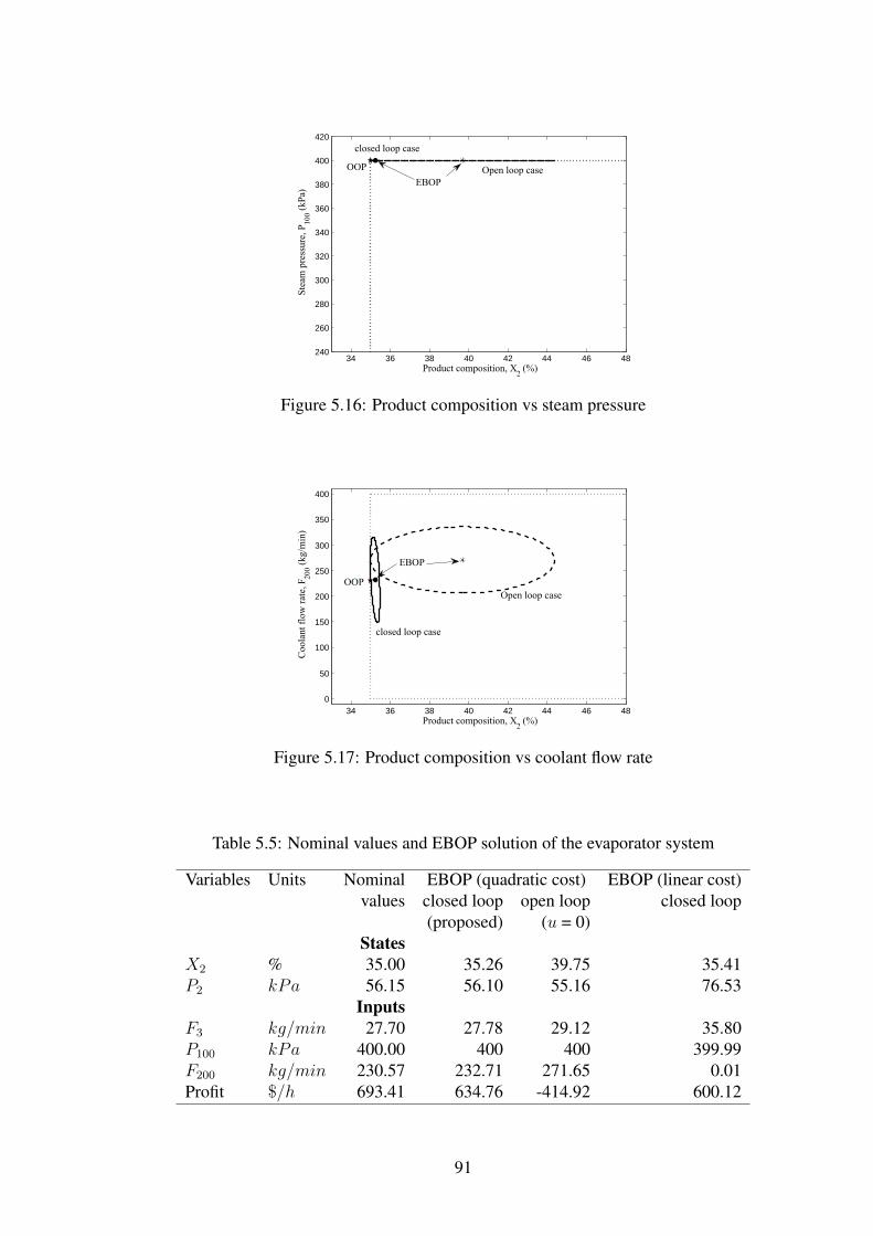
34 36 38 40 42 44 46 48240

260

280

300

320

340

360

380

400

420

Product composition, X2 (%)

Stea

m p

ress

ure,

P10

0 (kPa

)

EBOPOpen loop case

closed loop case

OOP

Figure 5.16: Product composition vs steam pressure

34 36 38 40 42 44 46 480

50

100

150

200

250

300

350

400

Product composition, X2 (%)

Coo

lant

flow

rate

, F20

0 (kg/

min

)

OOP

EBOP

Open loop case

closed loop case

Figure 5.17: Product composition vs coolant flow rate

Table 5.5: Nominal values and EBOP solution of the evaporator system

Variables Units Nominal EBOP (quadratic cost) EBOP (linear cost)values closed loop open loop closed loop

(proposed) (u = 0)States

X2 % 35.00 35.26 39.75 35.41P2 kPa 56.15 56.10 55.16 76.53

InputsF3 kg/min 27.70 27.78 29.12 35.80P100 kPa 400.00 400 400 399.99F200 kg/min 230.57 232.71 271.65 0.01Profit $/h 693.41 634.76 -414.92 600.12

91

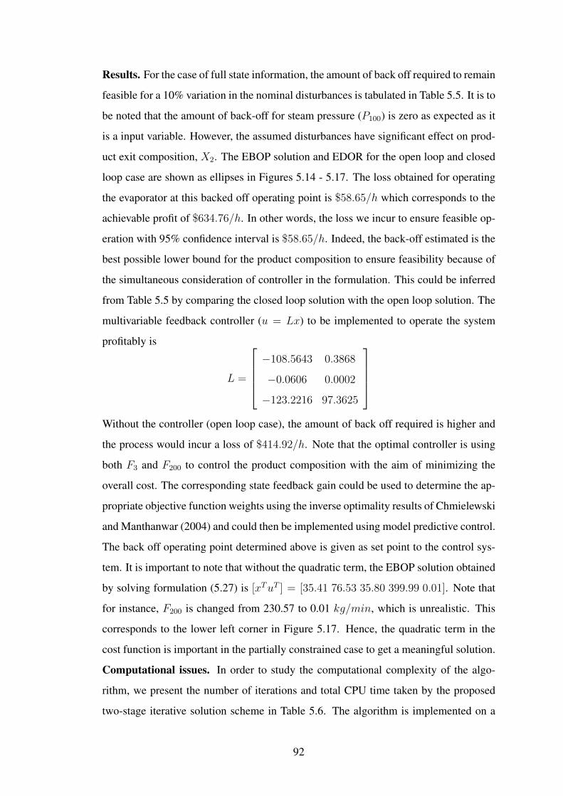
Results. For the case of full state information, the amount of back off required to remain

feasible for a 10% variation in the nominal disturbances is tabulated in Table 5.5. It is to

be noted that the amount of back-off for steam pressure (P100) is zero as expected as it

is a input variable. However, the assumed disturbances have significant effect on prod-

uct exit composition, X2. The EBOP solution and EDOR for the open loop and closed

loop case are shown as ellipses in Figures 5.14 - 5.17. The loss obtained for operating

the evaporator at this backed off operating point is $58.65/h which corresponds to the

achievable profit of $634.76/h. In other words, the loss we incur to ensure feasible op-

eration with 95% confidence interval is $58.65/h. Indeed, the back-off estimated is the

best possible lower bound for the product composition to ensure feasibility because of

the simultaneous consideration of controller in the formulation. This could be inferred

from Table 5.5 by comparing the closed loop solution with the open loop solution. The

multivariable feedback controller (u = Lx) to be implemented to operate the system

profitably is

L =

−108.5643 0.3868

−0.0606 0.0002

−123.2216 97.3625

Without the controller (open loop case), the amount of back off required is higher and

the process would incur a loss of $414.92/h. Note that the optimal controller is using

both F3 and F200 to control the product composition with the aim of minimizing the

overall cost. The corresponding state feedback gain could be used to determine the ap-

propriate objective function weights using the inverse optimality results of Chmielewski

and Manthanwar (2004) and could then be implemented using model predictive control.

The back off operating point determined above is given as set point to the control sys-

tem. It is important to note that without the quadratic term, the EBOP solution obtained

by solving formulation (5.27) is [xTuT ] = [35.41 76.53 35.80 399.99 0.01]. Note that

for instance, F200 is changed from 230.57 to 0.01 kg/min, which is unrealistic. This

corresponds to the lower left corner in Figure 5.17. Hence, the quadratic term in the

cost function is important in the partially constrained case to get a meaningful solution.

Computational issues. In order to study the computational complexity of the algo-

rithm, we present the number of iterations and total CPU time taken by the proposed

two-stage iterative solution scheme in Table 5.6. The algorithm is implemented on a

92

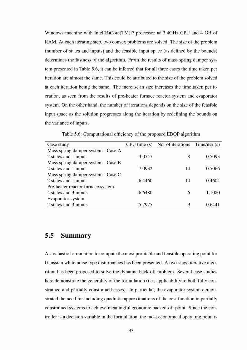
Windows machine with Intel(R)Core(TM)i7 processor @ 3.4GHz CPU and 4 GB of

RAM. At each iterating step, two convex problems are solved. The size of the problem

(number of states and inputs) and the feasible input space (as defined by the bounds)

determines the fastness of the algorithm. From the results of mass spring damper sys-

tem presented in Table 5.6, it can be inferred that for all three cases the time taken per

iteration are almost the same. This could be attributed to the size of the problem solved

at each iteration being the same. The increase in size increases the time taken per it-

eration, as seen from the results of pre-heater furnace reactor system and evaporator

system. On the other hand, the number of iterations depends on the size of the feasible

input space as the solution progresses along the iteration by redefining the bounds on

the variance of inputs.

Table 5.6: Computational efficiency of the proposed EBOP algorithm

Case study CPU time (s) No. of iterations Time/iter (s)Mass spring damper system - Case A2 states and 1 input 4.0747 8 0.5093Mass spring damper system - Case B2 states and 1 input 7.0932 14 0.5066Mass spring damper system - Case C2 states and 1 input 6.4460 14 0.4604Pre-heater reactor furnace system4 states and 3 inputs 6.6480 6 1.1080Evaporator system2 states and 3 inputs 5.7975 9 0.6441

5.5 Summary

A stochastic formulation to compute the most profitable and feasible operating point for

Gaussian white noise type disturbances has been presented. A two-stage iterative algo-

rithm has been proposed to solve the dynamic back-off problem. Several case studies

here demonstrate the generality of the formulation (i.e., applicability to both fully con-

strained and partially constrained cases). In particular, the evaporator system demon-

strated the need for including quadratic approximations of the cost function in partially

constrained systems to achieve meaningful economic backed-off point. Since the con-

troller is a decision variable in the formulation, the most economical operating point is

93

determined which, in fact, gives the best possible lower bound of the achievable profit.

The formulation can be extended to include measurement noise as an additional source

of uncertainty.

94

CHAPTER 6

ECONOMIC PERFORMANCE OF MODEL

PREDICTIVE CONTROL FOR CONSTRAINED

PROCESSES

In this chapter, we address the economic performance of MPC while operating at eco-

nomically backed-off operating point. For this purpose, we revisit the economic back-

off selection problem presented in Chapter 5, in discrete time framework. Recall that

the operation at constrained optimal point will result in infeasibility, and hence the se-

lection of an economically optimal yet dynamically feasible operating point is vital for

efficient operation. The basic idea in set point selection based on economic back-off

is that the dynamic operating region should have the least variability in the active con-

strained variables while ensuring feasibility of other variables. In other words, the dy-

namic operating region is oriented by proper design of a linear multivariable controller

such that the variability in active constrained variables are as low as possible. This con-

troller design can be transformed into an equivalent objective function weights of the

MPC controller. Demonstrative case studies are presented to illustrate the economic

performance of the MPC controller at economic back-off point.

6.1 Introduction

In a typical chemical process, the plant-wide control is carried out in a two-layer hi-

erarchial setting: the upper real time optimization layer determines the operating point

by minimizing an economic cost function subject to steady state model of the pro-

cess; whereas the lower control layer steers the plant to the computed optimal point

despite disturbances entering the process (Aske et al., 2008). Model Predictive Control

(MPC) is one of the successfully employed techniques in the control layer because of

its ability to handle constraints, its direct applicability to multivariable systems and its

potential benefit in improving the economic performance of the plant. In the standard

MPC problem, the process is regulated at the optimal steady state point compensating

for the undesirable disturbances and hence minimizes the cost function that measures

the deviation from the steady state point. This framework relies on two fundamental

assumptions: Firstly, the operating point lies in the interior of the feasible region to

guarantee feasibility of the control problem and secondly, only steady state effect on

economics is considered to be important and hence the economic benefit one could

achieve during transients is ignored. However, optimizing for process economics under

steady state conditions may tend to operate the process plant at the boundary of the fea-

sible region. Therefore, the focus of this chapter is to present the MPC framework for

nominally constrained processes and discuss the notion of profitability during transient

operation.

Maximizing profitability of the plant at steady state may require one to operate at

the constrained optimal point. For the case of active state or output constraints at the

optimal point, uncertainties such as disturbances, modelling errors and measurement

errors might cause frequent violation of the constraints. Consequently, it leads to ex-

ceeding environmental limits, producing inferior quality products and at times result in

unsafe process conditions. In other words, the set point decided on the basis of steady

state model of the process may not be robust enough to handle dynamic conditions

caused by the uncertain process environments. As a result, it is difficult to guarantee

feasibility of the control problem. In order to address the infeasibility issue, Scokaert

and Rawlings (1999) have developed two approaches that reduces both the magnitude

and duration of constraint violations. In the first approach (optimized minimal time),

the performance is Pareto optimal, that is, the magnitude of constraint violation is min-

imal and consistent with the faster return of the state. In the second approach (soft

constrained MPC), the use of sum of linear and quadratic penalty terms at each time

step guarantees the control algorithm to have a solution, however, even when the state

constraints can be satisfied, the soft-constraint law may not enforce the state constraints

and unnecessary violations may still result. On the other hand, in addition to the prob-

lem of infeasible operation, the input constraints being active at the optimal point might

result in unreachable target values for some set of disturbances. In this regard, Rao

and Rawlings (1999) have demonstrated for the case of constant step-like disturbances,

96

the possibility of unreachable target values due to input saturation and infeasible oper-

ations. Therefore, they proposed a modified MPC algorithm which involves updating

the reachable target values before determining the optimal input sequence at every time

step. The target values are computed by solving a quadratic programming problem us-

ing exact penalties for the estimated values of states and disturbances. The problem

of target calculation, to handle model uncertainties, is casted as a second order cone

programming problem. In summary, although regulating the plant at the active con-

straints will be profitable, it poses difficulty in operation due to constraint violations.

To circumvent this infeasibility issue, we presented the back-off approach in Chapter 5.

To gain economic advantage during transients, very recently there is increasing in-

terest in Economic Model Predictive Control, by coupling the two-layer structure into a

single layer that directly optimizes the economic objective at each time step. Unlike the

quadratic cost function of the standard MPC problem, the economic cost function can

be non-linear and non-convex, in general. Therefore, the existing MPC properties are no

longer valid. Hence, to establish the closed loop properties (such as convergence and

nominal asymptotic stability) of the economic MPC problem, Rawlings et al. (2008)

proposed a terminal constraint MPC formulation, in which the system is driven to opti-

mal steady state point at the end of the horizon. The receding horizon implementation

of the terminal constraint MPC is demonstrated for the case of unreachable set points

due to input constraints. The asymptotic stability result was also presented for terminal

penalty MPC by introducing rotated stage cost. Later, Diehl et al. (2011) presented

a Lyapunov function for the economic MPC problems with terminal constraints that

satisfy strong duality assumption of the steady state problem to establish asymptotic

stability of the closed loop system. Similar Lyapunov based stability analysis for the

terminal penalty formulation was established by imposing a region constraint on the

terminal state (Amrit et al., 2011). Further, they showed that strict dissipativity is suf-

ficient for guaranteeing asymptotic stability of the closed loop system. In Angeli et al.

(2012), the average control performance of the eMPC was shown to outperform the

optimal steady state economic performance.

In this chapter, we work within the MPC framework for the case of active state

or input constraints. For this purpose, we adapt the economic back-off approach pre-

97

sented in the previous chapter, to determine the most profitable operating point. The

benefit of this approach is that the optimal multivariable controller, that can achieve the

profitability without constraint violations, comes as part of the solution. This optimal

multivariable controllers can be tailored to be used in MPC framework using inverse

optimality results. Finally, illustrations are provided to demonstrate the performance of

MPC using the proposed approach.

6.2 Standard MPC vs Economic MPC

Consider the discrete-time, constrained dynamic system of the form

sk+1 = f(sk,mk, pk) (6.1a)

vk = h(sk,mk, pk) (6.1b)

vmin ≤ vk ≤ vmax (6.1c)

with state variables sk ∈ Rnx , manipulated inputs mk ∈ Rnu and disturbances pk ∈

Rnd . The input and output constraints are accounted in vector, vk. In general, the pro-

cess plants are operated at the steady state point that will yield maximum profit. Typ-

ically this operating point is determined by solving a non-linear optimization problem

for the nominal values of disturbances (p0) with negated profit function, J as objective

and the vector valued functions, f and h, denote the steady state model of the process

and performance bounds on the variables, respectively. Mathematically, the steady state

optimization problem can be expressed as

minms

J(ss,ms, p0) (6.2a)

s.t. ss = f(ss,ms, p0) (6.2b)

vs = h(ss,ms, p0) (6.2c)

vmin ≤ vs ≤ vmax (6.2d)

The optimal solution is denoted by {s∗s,m∗s}. It can be either unconstrained or con-

strained. However, if some of the bound constraints are active at the optimal solution,

98

then there might be violation of constraints for some other values of disturbance vari-

ables. If the manipulated inputs are constrained, they typically correspond to physical

limitations. On the other hand, if the state variables are constrained, they correspond to

safety and performance degradations. Therefore, it is difficult to operate at this nomi-

nally constrained optimal point without performance degradation or infeasibility issues.

In continuous processes, the plant has to be regulated at the economically optimal

steady state point despite disturbances for achieving maximum profit. MPC can be

successfully deployed for this purpose. The general philosophy of MPC is to utilize the

dynamic plant model to predict the transients and determine the optimal input sequence

that minimizes the departure from the optimal steady state point. The MPC controller,

however, implements only the first of the input sequence at the current time instant.

In the next time instant, the current measurements give feedback information to the

controller and solve for the next set of optimal input sequence in a receding horizon

fashion (Maciejowski, 2002; Qin and Badgwell, 2003; Rawlings and Mayne, 2009).

Let us define deviation variables with respect to the nominally optimal point: xk =

sk − s∗s, uk = mk −m∗s, and dk = pk − p0. Linearizing around the nominal point, the

dynamic process model can be expressed as

xk+1 = Adxk +Bduk +Gddk (6.3)

where Ad, Bd and Gd are the partial derivative of f evaluated at (s∗s,m∗s, p0). Similar

development on the output vector vk (i.e., denoting zk = vk − v∗s ) yields

zk = Zxxk + Zuuk + Zddk (6.4a)

zmin ≤ z ≤ zmax (6.4b)

where Zx, Zu and Zd are the partial derivative of h evaluated at (s∗s,m∗s, p0). In a

standard MPC formulation, the objective function is a measure of the weighted sum

of squares of deviation of the dynamic values of the state and input, (sk,mk), from the

optimal steady state point, (s∗s,m∗s). Therefore, in terms of deviation variables, the plant

99

has to be regulated at the origin. This objective can be mathematically expressed as:

`(xk, uk) = xTkQxk + uTkRuk (6.5)

with Q � 0 and R � 0. For the control horizon of N moves, we can denote the overall

stage cost as Φ(x, u) =∑N−1

k=0 `(xk, uk). The MPC regulation problem with terminal

constraints can be now stated as:

minu

Φ(x, u) (6.6a)

s.t. xk+1 = Adxk +Bduk +Gddk, k = 0 to N − 1 (6.6b)

dk+i = dk, ∀k + i > k (6.6c)

zk = Zxxk + Zuuk + Zddk (6.6d)

zmin ≤ zk ≤ zmax (6.6e)

xN = 0 (6.6f)

The terminal constraint on the state variables enforces stability of the MPC problem. Al-

ternately, the terminal penalty can be included in the cost function such that ΦN(xN) =

xTNPxN , where P is the terminal penalty matrix. The resulting optimal input sequence

that takes the state from x0 to origin, is given by

u∗ = {u∗0, u∗1, . . . , u∗N−1} (6.7)

and the corresponding state sequence is given by

x∗ = {x∗1, x∗2, . . . , x∗N} (6.8)

However, the MPC control law implements only the first input move of the optimal

input sequence, and it can be expressed as

umpc = u∗0(x) (6.9)

We assume that the measurement of the state variables are available accurately. Given

the current values of state variables as feedback information to the controller, the op-

100

timization problem is resolved to find the new set of optimal input sequence. At each

time step, the MPC controller requires one to solve a quadratic programming problem

for which efficient algorithms like active set or interior point methods are available

(Nocedal and Wright, 2006). Notice that Q and R are the tuning parameters in the

controller. Choosing large values of Q in comparison to R, will allow for large control

actions and quickly drive the state to the optimal steady state point. Conversely, choos-

ing large values of R relative to Q will penalize for large control action and slow down

the rate at which the state approaches the optimal operating point. Hence, appropriate

selection of the tuning parameters is necessary for better control.

Alternately, one can choose the operational cost of the plant defined in (6.2a) as

MPC stage cost. This will directly optimize for the dynamic economic performance

rather than regulating the plant at the optimal steady state point. However, to ensure

stability and convergence, terminal constraints on the state variables can be set as the

optimal operating point. Taking the stage cost as `(xk, uk) = J(xk, uk), the economic

MPC formulation with terminal constraints can be expressed as:

minu

Φeco(x, u) =N−1∑k=0

J(xk, uk) (6.10a)

s.t. xk+1 = Adxk +Bduk +Gddk, k = 0 to N − 1 (6.10b)

dk+i = dk, ∀k + i > k (6.10c)

zk = Zxxk + Zuuk + Zddk (6.10d)

zmin ≤ zk ≤ zmax (6.10e)

xN = 0 (6.10f)

The direct use of an economic objective function as MPC cost enables one to determine

the economically optimal input sequence at each time step. In other words, economic

MPC couples the two-layer hierarchical setting of the traditional plant-wide control

structure into a single layer. Further, it can also be interpreted as optimizing the in-

put sequence for the current value of disturbance, rather than for the nominal value of

disturbance as in standard MPC problem. Although one can achieve economic advan-

tage during transients, the stability and robustness properties are still required for the

general non-linear form of the economic cost. Some of the recent works, along these

101

lines, established that dissipativity is sufficient for guaranteeing asymptotic stability

of the closed loop system (Angeli et al., 2012; Rawlings et al., 2012). For a general

non-convex economic objective, the regularization terms are often added to achieve

dissipativity. However, it was advocated in Biegler (2013) that the plant operation is

easier to monitor and manage at steady state conditions. Further, stability and robust-

ness properties can be easily analyzed under steady state assumptions.

6.3 Target selection using economic back-off approach

In this section, we present an algorithm to determine the most profitable operating point

(i.e., economic back-off point) in the presence of random Gaussian white noise dis-

turbances for optimally constrained, discrete-time processes. First, we present the op-

timization formulation involving conic constraints to obtain the economic backed-off

point. The resulting formulation contains a non-linear matrix equality, which makes

the resulting optimization problem as non-convex. Therefore, finally we present the

iterative solution procedure to obtain the economic back-off point.

6.3.1 Problem formulation

The objective of this subsection is to present the optimization formulation that finds

the economically optimal backed-off operating point by a suitable controller design.

Typically, this requires one to solve a dynamic optimization problem involving differ-

ential constraints (Figueroa et al., 1996; Mohideen et al., 1996). Owing to the infinite-

dimensional nature of the problem and higher computational cost, we propose to present

an alternate Lyapunov based stochastic approach. For this purpose, we make the fol-

lowing assumptions:

• Disturbances are the only source of uncertainty considered and they are charac-terized by Gaussian white noise process with zero mean and known variances.

• The set of active constraints do not change over the assumed disturbance magni-tude.

• The dynamic behavior of the system is described by a linear, discrete-time, statespace model.

102

• Complete information about the states are available at any instant of time.

• A linear multi-variable controller with full state information (uk = Ldxk) is avail-able for feedback.

Following the definition of deviation variables as presented in previous section and

assuming zero mean Gaussian white noise type of disturbance vector, we have dss = 0.

Now, the steady state process model can be expressed as

xss = Adxss +Bduss (6.11)

Similar development on the output vector z yields

zss = Zxxss + Zuuss (6.12a)

zmin ≤ zss ≤ zmax (6.12b)

Recall that the selection of backed-off operating point should result in dynamic feasi-

bility and hence defining the new deviation variables around the back-off point to define

the dynamics: x = x− xss, u = u− uss, we can write the following discrete-time linear

state space model and the performance constraints as

xk+1 = Adxk +Bduk +Gddk (6.13)

zk = Zxxk + Zuuk + Zddk (6.14)

zmin − zss ≤ zk ≤ zmax − zss (6.15)

Our objective is to determine the backed-off operating point that minimizes the loss in

operational profit while ensuring the feasible process dynamics. For this purpose, we

assume a linear multivariable controller of the form, uk = Ldxk. The system dynamics

around the back-off point can be described using closed loop steady state covariance

matrix of the state vector (Σx := E[xTk xk]), which is a symmetric positive semi-definite

solution to the Lyapunov equation,

Σx = (Ad +BdLd)Σx(Ad +BdLd)T +GdΣdG

Td (6.16)

where Σd is the diagonal matrix denoting the variances of the disturbance variables.

103

Similar development of the signal zk yields

Σz = (Zx + ZuLd)Σx(Zx + ZuLd)T + ZdΣdZd

T (6.17)

It is important to notice that the covariance, Σz can be geometrically inferred as ellip-

soids that approximates the dynamic operating region with backed-off operating point

as center. Denoting Σz = P 2, the ellipsoidal description of the operating region can be

expressed as

E = {zss + αPz | ‖z‖2 ≤ 1} (6.18)

where P is the positive square root of Σz and α depends on the confidence limit (e.g., for

a confidence limit of 95%, α = 2). Notice that z = zss + αPz. Therefore, we enforce

dynamic feasibility by finding the ellipsoid within the performance bounds which is

given by

E = {(zmin ≤ zss + αPz ≤ zmax) | ‖z‖2 ≤ 1} (6.19)

This representation ensures that the whole ellipsoid should lie within the performance

bounds. Thus, the problem can be restated as finding the center of the ellipsoid close

to the optimal operating point such that the ellipsoid is contained within performance

bounds.

Theorem 6.3.1 (Peng et al., 2005) ∃ stabilizingLd,X � 0 s.t. Σx = (Ad+BdLd)Σx(Ad+

BdLd)T +GdΣdG

Td and Σz = (Zx +ZuLd)Σx(Zx +ZuLd)

T +ZdΣdZdT if and only if

∃ Y , X � 0 and Z � 0 s.t. X −GdΣdGTd (AdX +BdY )

(AdX +BdY )T X

� 0, Z − ZdΣdZdT ZxX + ZuY

(ZxX + ZuY )T X

� 0.

For proof of the above theorem, the reader is referred to (Peng et al., 2005).

Application of Theorem 5.2.3 recasts the infinite dimensional dynamic feasibility

constraints as finite dimensional second order cone constraints which can be solved

very efficiently using existing tools (Löfberg, 2004). Application of Theorem 6.3.1

ensures that the stabilizing multivariable controller for the process can be found. Hence,

the final formulation of the discrete time economic back-off selection problem can be

104

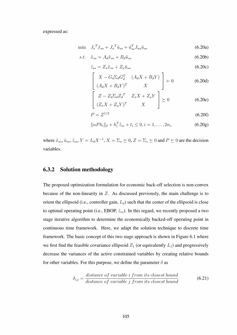
expressed as:

min JxT xss + Ju

T uss + uTssJuuuss (6.20a)

s.t. xss = Adxss +Bduss (6.20b)

zss = Zxxss + Zuuss (6.20c) X −GdΣdGTd (AdX +BdY )

(AdX +BdY )T X

� 0 (6.20d)

Z − ZdΣdZdT ZxX + ZuY

(ZxX + ZuY )T X

� 0 (6.20e)

P = Z1/2 (6.20f)

‖αPhi‖2 + hTi zss + ti ≤ 0, i = 1, . . . , 2nz (6.20g)

where xss, uss, zss, Y = LdX−1,X = Σx � 0, Z = Σz � 0 and P � 0 are the decision

variables.

6.3.2 Solution methodology

The proposed optimization formulation for economic back-off selection is non-convex

because of the non-linearity in Z. As discussed previously, the main challenge is to

orient the ellipsoid (i.e., controller gain, Ld) such that the center of the ellipsoid is close

to optimal operating point (i.e., EBOP, zss). In this regard, we recently proposed a two

stage iterative algorithm to determine the economically backed-off operating point in

continuous time framework. Here, we adapt the solution technique to discrete time

framework. The basic concept of this two stage approach is shown in Figure 6.1 where

we first find the feasible covariance ellipsoid Z1 (or equivalently L1) and progressively

decrease the variances of the active constrained variables by creating relative bounds

for other variables. For this purpose, we define the parameter δ as

δi,j =distance of variable i from its closest bound

distance of variable j from its closest bound(6.21)

105

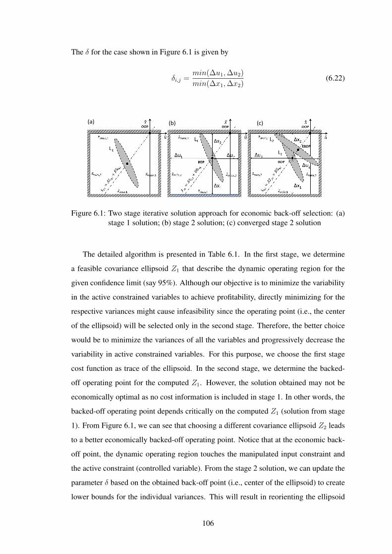
The δ for the case shown in Figure 6.1 is given by

δi,j =min(∆u1,∆u2)

min(∆x1,∆x2)(6.22)

(a) (b) (c)

Figure 6.1: Two stage iterative solution approach for economic back-off selection: (a)stage 1 solution; (b) stage 2 solution; (c) converged stage 2 solution

The detailed algorithm is presented in Table 6.1. In the first stage, we determine

a feasible covariance ellipsoid Z1 that describe the dynamic operating region for the

given confidence limit (say 95%). Although our objective is to minimize the variability

in the active constrained variables to achieve profitability, directly minimizing for the

respective variances might cause infeasibility since the operating point (i.e., the center

of the ellipsoid) will be selected only in the second stage. Therefore, the better choice

would be to minimize the variances of all the variables and progressively decrease the

variability in active constrained variables. For this purpose, we choose the first stage

cost function as trace of the ellipsoid. In the second stage, we determine the backed-

off operating point for the computed Z1. However, the solution obtained may not be

economically optimal as no cost information is included in stage 1. In other words, the

backed-off operating point depends critically on the computed Z1 (solution from stage

1). From Figure 6.1, we can see that choosing a different covariance ellipsoid Z2 leads

to a better economically backed-off operating point. Notice that at the economic back-

off point, the dynamic operating region touches the manipulated input constraint and

the active constraint (controlled variable). From the stage 2 solution, we can update the

parameter δ based on the obtained back-off point (i.e., center of the ellipsoid) to create

lower bounds for the individual variances. This will result in reorienting the ellipsoid

106

Table 6.1: Algorithm for selecting economic back-off operating point for discrete timeprocess

1 Initialize the parameter δi,j = 0.2 Find Z by solving the following convex problem (Stage 1),

minX�0,Z�0,Y

Tr(Z)

s.t.

[X −GdΣdG

Td (AdX +BdY )

(AdX +BdY )T X

]� 0[

Z − ZdΣdZdT ZxX + ZuY

(ZxX + ZuY )T X

]� 0

σ2z,i <

1

4α2(zmax,i − zmin,i)2; i = 1 · · ·nz

σ2z,i >

δ2i,j

α2σ2z,j; i = 1, j − 1, j + 1, nz

If no feasible Z can be found, exit.3 Compute P = Z1/2. Find the BOP (zss) by solving the following convex

problem (Stage 2),

minxss,uss,zss

JxT xss + Ju

T uss + uTssJuuuss

s.t. xss = Adxss +Bduss

zss = Zxxss + Zuuss

‖αPhi‖2 + hTi zss + ti ≤ 0, i = 1, . . . , 2nz

4 Terminate on convergence. Otherwise, update δi,j using (6.21) from the currentvalue of BOP and proceed to Step 2.

107

(i.e., designing a better controller) that has reduced variability in active constrained

variables on subsequent iterations. This procedure is iterated until convergence. Notice

that both the stage requires one to solve convex problems, which could be easily solved

using CVX, a package for specifying and solving convex programs (Grant and Boyd,

2011).

6.4 MPC regulation at economic back-off point

In the previous section, we presented a method to determine the economical and dynam-

ically feasible operating point along with the optimal linear multivariable controller.

Though there exist different controllers that define the dynamic operating region, the

one that gives the minimal loss in profit, due to backing-off, is determined. Therefore,

the aim of this section is to utilize this economically backed-off operating point as set

point in the MPC controller. Recall that the backed-off operating point is both economi-

cal and dynamically feasible in the presence of the obtained multivariable controller. In

other words, the economic back-off point is statistically guaranteed to be profitable and

feasible within the expected dynamic operating region, only if we employ the deviced

multivariable controller. Therefore, the present challenge is on utilizing the designed

multivariable controller within the MPC framework. To this end, we invoke the follow-

ing inverse optimality result that finds the equivalent objective function weights of the

MPC controller given the multivariable controller.

Theorem 6.4.1 (Chmielewski and Manthanwar, 2004) If ∃ P � 0 and R � 0 s.t. P − ATdPAd + LTd (R +BTd PBd)Ld −LTd (R +BT

d PBd)− ATdPBd

−(R +BTd PBd)Ld −BT

d PAd R

� 0

then Q=P −ATdPAd + LTd (R+BTd PBd)Ld and M=− LTd (R+BT

d PBd)−ATdPBd

will be s.t. Q M

MT R

� 0

and P and Ld will satisfy P = ATdPAd + Q − (M + ATdPBd)(R + BTd PBd)

−1(M +

ATdPBd)T and Ld = −(R + BT

d PBd)−1(M + ATdPBd)

T . For proof of the above

108

theorem, the reader is referred to (Chmielewski and Manthanwar, 2004).

Given the system matrices, {Ad, Bd} and the controller gain matrix, Ld, application of

Theorem 6.4.1 will yield the objective function weights of the MPC controller (Ahmed

and Chmielewski, 2013). Notice that the multivarible controller obtained from the pro-

posed economic back-off formulation can be inferred as the LQR controller satisfying

the constraints within the prescribed probability. In other words, the operation at the

economic back-off point with the obtained multivariable controller will result in the

(unconstrained) LQR solution in statistical sense. Therefore, the obtained multivariable

controller is identical to the unconstrained MPC solution with infinite horizon. There-

fore, the objective function weights will result in the operating region identical to that

of the multivariable controller. In this work, we utilize this objective function weights

with finite horizon approximation in the standard MPC framework. Denoting the ob-

jective function as the deviation from the economically backed-off operating point, we

can define

`ebop(xk, uk) = xTkQxk + xTkMuk + uTkRuk (6.23)

The economically optimal MPC regulation framework can now be casted as:

minu

Φebop(x,u) =N−1∑k=0

`ebop(xk, uk) (6.24a)

s.t. xk+1 = Adxk +Bduk +Gddk, k = 0 to N − 1 (6.24b)

zk = Zxxk + Zuuk + Zddk, dk ∼ N (0,Σd) (6.24c)

zmin ≤ zk ≤ zmax (6.24d)

xN = xss (6.24e)

This approach is compatible with the standard MPC framework, where a quadratic pro-

gramming problem is solved at each time step. The main benefit of this approach is

that the profitable dynamic operating region is naturally accomplished by this choice

of tuning parameters because the controller is designed by minimizing the variability

of the active constrained variables. Hence, the dynamic economic benefits can also be

attained within this framework.

109

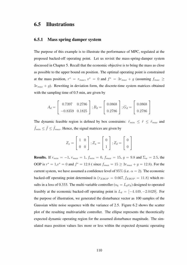
6.5 Illustrations

6.5.1 Mass spring damper system

The purpose of this example is to illustrate the performance of MPC, regulated at the

proposed backed-off operating point. Let us revisit the mass-spring-damper system

discussed in Chapter 5. Recall that the economic objective is to bring the mass as close

as possible to the upper bound on position. The optimal operating point is constrained

at the mass position, r∗ = rmax, v∗ = 0 and f ∗ = 3rmax + g (assuming fmax ≥

3rmax + g). Rewriting in deviation form, the discrete-time system matrices obtained

with the sampling time of 0.5 min, are given by

Ad =

0.7397 0.2786

−0.8359 0.1825

;Bd =

0.0868

0.2786

;Gd =

0.0868

0.2786

The dynamic feasible region is defined by box constraints: rmin ≤ r ≤ rmax and

fmin ≤ f ≤ fmax. Hence, the signal matrices are given by

Zx =

1 0

0 0

;Zu =

0

1

;Zd =

0

0

Results. If rmin = −1, rmax = 1, fmin = 0, fmax = 15, g = 9.8 and Σw = 2.5, the

OOP is r∗ = 1,v∗ = 0 and f ∗ = 12.8 ( since fmax = 15 ≥ 3rmax + g = 12.8). For the

current system, we have assumed a confidence level of 95% (i.e. α = 2). The economic

backed-off operating point determined is (rEBOP = 0.667, fEBOP = 11.8) which re-

sults in a loss of 0.333. The multi-variable controller (uk = Ldxk) designed to operated

feasibly at the economic backed-off operating point is Ld = [−4.449,−2.0429]. For

the purpose of illustration, we generated the disturbance vector as 100 samples of the

Gaussian white noise sequence with the variance of 2.5. Figure 6.2 shows the scatter

plot of the resulting multivariable controller. The ellipse represents the theoretically

expected dynamic operating region for the assumed disturbance magnitude. The sim-

ulated mass position values lies more or less within the expected dynamic operating

110

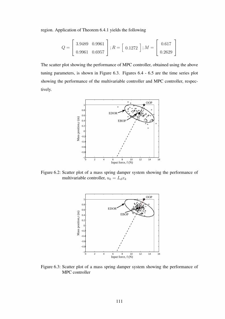
region. Application of Theorem 6.4.1 yields the following

Q =

3.9489 0.9961

0.9961 0.6957

;R =[

0.1272]

;M =

0.617

0.2629

The scatter plot showing the performance of MPC controller, obtained using the above

tuning parameters, is shown in Figure 6.3. Figures 6.4 - 6.5 are the time series plot

showing the performance of the multivariable controller and MPC controller, respec-

tively.

0 2 4 6 8 10 12 14 16−1

−0.8

−0.6

−0.4

−0.2

0

0.2

0.4

0.6

0.8

1

Input force, f (N)

Mas

s po

sitio

n,r

(m)

OOP

EBOP

EDOR

Figure 6.2: Scatter plot of a mass spring damper system showing the performance ofmultivariable controller, uk = Ldxk

0 2 4 6 8 10 12 14 16−1

−0.8

−0.6

−0.4

−0.2

0

0.2

0.4

0.6

0.8

1

Input force, f (N)

Mas

s po

sitio

n,r

(m)

EBOP

OOP

EDOR

Figure 6.3: Scatter plot of a mass spring damper system showing the performance ofMPC controller

111

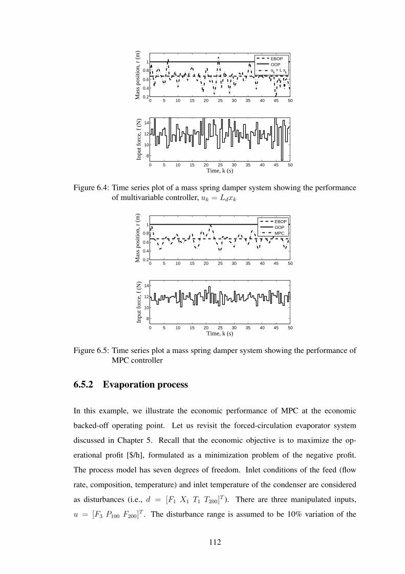
0 5 10 15 20 25 30 35 40 45 500.2

0.4

0.6

0.8

1

Mas

s po

sitio

n, r

(m

)

EBOPOOPuk = L xk

0 5 10 15 20 25 30 35 40 45 50

8

10

12

14

Inpu

t for

ce, f

(N

)

Time, k (s)

Figure 6.4: Time series plot of a mass spring damper system showing the performanceof multivariable controller, uk = Ldxk

0 5 10 15 20 25 30 35 40 45 500.2

0.4

0.6

0.8

1

Mas

s po

sitio

n, r

(m

)

EBOPOOPMPC

0 5 10 15 20 25 30 35 40 45 50

8

10

12

14

Inpu

t for

ce, f

(N

)

Time, k (s)

Figure 6.5: Time series plot a mass spring damper system showing the performance ofMPC controller

6.5.2 Evaporation process

In this example, we illustrate the economic performance of MPC at the economic

backed-off operating point. Let us revisit the forced-circulation evaporator system

discussed in Chapter 5. Recall that the economic objective is to maximize the op-

erational profit [$/h], formulated as a minimization problem of the negative profit.

The process model has seven degrees of freedom. Inlet conditions of the feed (flow

rate, composition, temperature) and inlet temperature of the condenser are considered

as disturbances (i.e., d = [F1 X1 T1 T200]T ). There are three manipulated inputs,

u = [F3 P100 F200]T . The disturbance range is assumed to be 10% variation of the

112

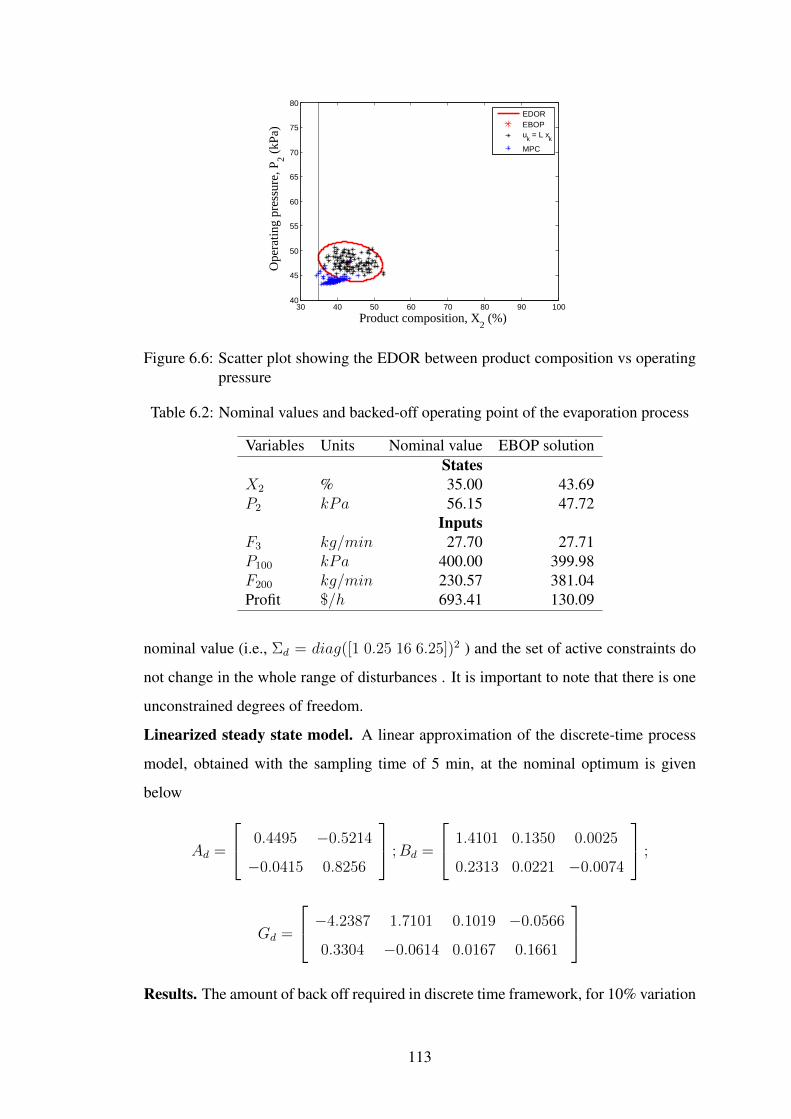
30 40 50 60 70 80 90 10040

45

50

55

60

65

70

75

80

Product composition, X2 (%)

Ope

ratin

g pr

essu

re, P

2 (kP

a)

EDOREBOPuk = L xk

MPC

Figure 6.6: Scatter plot showing the EDOR between product composition vs operatingpressure

Table 6.2: Nominal values and backed-off operating point of the evaporation process

Variables Units Nominal value EBOP solutionStates

X2 % 35.00 43.69P2 kPa 56.15 47.72

InputsF3 kg/min 27.70 27.71P100 kPa 400.00 399.98F200 kg/min 230.57 381.04Profit $/h 693.41 130.09

nominal value (i.e., Σd = diag([1 0.25 16 6.25])2 ) and the set of active constraints do

not change in the whole range of disturbances . It is important to note that there is one

unconstrained degrees of freedom.

Linearized steady state model. A linear approximation of the discrete-time process

model, obtained with the sampling time of 5 min, at the nominal optimum is given

below

Ad =

0.4495 −0.5214

−0.0415 0.8256

;Bd =

1.4101 0.1350 0.0025

0.2313 0.0221 −0.0074

;

Gd =

−4.2387 1.7101 0.1019 −0.0566

0.3304 −0.0614 0.0167 0.1661

Results. The amount of back off required in discrete time framework, for 10% variation

113

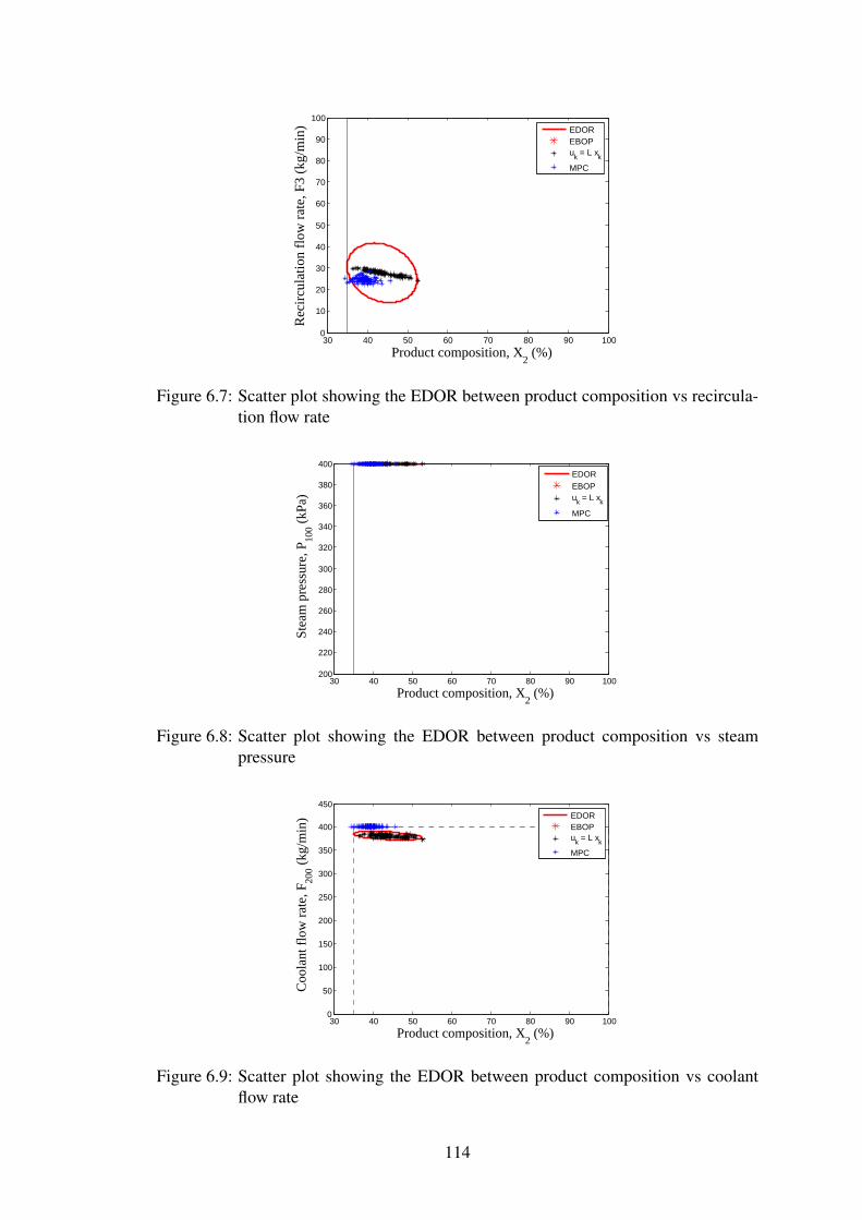
30 40 50 60 70 80 90 1000

10

20

30

40

50

60

70

80

90

100

Product composition, X2 (%)

Rec

ircu

latio

n fl

ow r

ate,

F3

(kg/

min

)

EDOREBOPuk = L xk

MPC

Figure 6.7: Scatter plot showing the EDOR between product composition vs recircula-tion flow rate

30 40 50 60 70 80 90 100200

220

240

260

280

300

320

340

360

380

400

Product composition, X2 (%)

Stea

m p

ress

ure,

P10

0 (kP

a)

EDOREBOPuk = L xk

MPC

Figure 6.8: Scatter plot showing the EDOR between product composition vs steampressure

30 40 50 60 70 80 90 1000

50

100

150

200

250

300

350

400

450

Product composition, X2 (%)

Coo

lant

flo

w r

ate,

F20

0 (kg

/min

)

EDOREBOPuk = L xk

MPC

Figure 6.9: Scatter plot showing the EDOR between product composition vs coolantflow rate

114

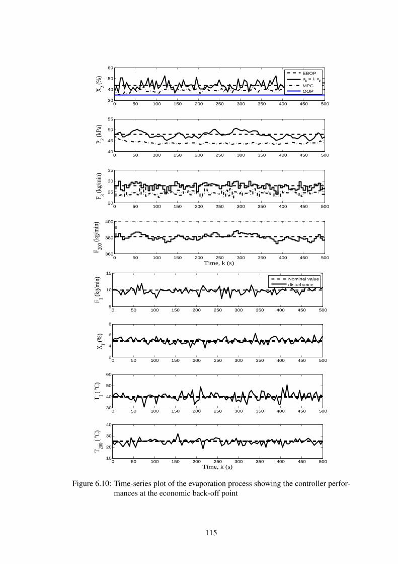
0 50 100 150 200 250 300 350 400 450 50030

40

50

60

X2 (%

)

EBOPuk = L xk

MPCOOP

0 50 100 150 200 250 300 350 400 450 50040

45

50

55

P2 (k

Pa)

0 50 100 150 200 250 300 350 400 450 50020

25

30

35

F 3 (kg/

min

)

0 50 100 150 200 250 300 350 400 450 500360

380

400

F 200 (k

g/m

in)

Time, k (s)

0 50 100 150 200 250 300 350 400 450 5005

10

15

F 1 (kg/

min

)

Nominal valuedisturbance

0 50 100 150 200 250 300 350 400 450 5002

4

6

8

X1 (%

)

0 50 100 150 200 250 300 350 400 450 50030

40

50

60

T 1 ( °C

)

0 50 100 150 200 250 300 350 400 450 50010

20

30

40

T 200 (

°C)

Time, k (s)

Figure 6.10: Time-series plot of the evaporation process showing the controller perfor-mances at the economic back-off point

115

in nominal values of disturbances, is tabulated in Table 6.2. The amount of achievable

profit at this economic back-off point is $ 130/h. Notice that the steam pressure (P100)

requires no back-off for the assumed disturbance magnitude and can be set at fully open

valve position. The multivariable feedback controller (uk = Ldxk) designed to operate

the system profitably is

Ld =

−0.3128 0.32224

0.0000 0.0000

−0.27626 2.1848

Application of Theorem 6.4.1 results in the following tuning matrices,

Q =

1.8455 −0.26981

−0.26981 2.9259

;R =

3.1648 −0.0004 −0.4441

−0.0004 3.4408 −0.0021

−0.4441 −0.0021 0.6318

;

M =

0.87607 0.00012 0.034883

−0.11931 −0.00179 −1.2314

Simulation was performed by generating 100 samples of disturbance variables, obtained

from zero mean Gaussian white noise sequences with variances of Σd. Scatter compar-

ing the performances of the resulting multivariable controller with MPC controller is

shown in Figures 6.6 - 6.9. The theoretically expected dynamic operating regions are

shown as ellipses. Recall that the center of the ellipse denotes the economic back-off

point. From Figure 6.9, we can observe that the theoretically required back-off value

for the coolant flow rate is necessary in case of multivariable controller. However, the

MPC controller always keeps the coolant flow rate at its maximum value. Further, it

should be noted that the MPC controller operates closer to the active constrained vari-

able (i.e., product composition) than the multivariable controller. Hence, the economic

performance of the MPC controller at the economic back-off point is better than the

multivariable controller. This can also be seen from the time series plot presented in

Figure 6.10.

116

6.6 Summary

In this chapter, we presented the MPC framework that addresses the economic perfor-

mance of the constrained process in the standard MPC framework. To accomplish this,

we obtained the optimal multivariable controller using the economic back-off approach

and transformed it into an equivalent MPC weighting matrices using inverse optimal-

ity results. The proposed approach is successfully demonstrated using a mass spring

damper system and an evaporator system.

117

CHAPTER 7

SIMULTANEOUS SELECTION OF BACKED-OFF

OPERATING POINT, CONTROLLER AND

MEASUREMENTS BASED ON ECONOMICS

Based on the paper presented in 12th European Control Conference

This chapter discusses the simultaneous selection of measurements and economic

backed off operating point when the nominal optimal operating point is constrained.

However, operation at this point becomes infeasible due to uncertainties. In Chap-

ter 5, we proposed an optimization formulation that determines the economic backed-

off point to ensure feasibility assuming accurate measurement of the states are available

and disturbance as the only source of uncertainty. Here, we extend the formulation to

partial state information case and also determine the optimal set of measurements for

economical operation. The formulation also finds a suitable multivariable controller

to achieve economic benefits. The final formulation is a mixed integer non-linear pro-

gram. Hence, we propose to use a branch and bound type solution such that a two stage

iterative problem is solved at each branching step. Finally, the proposed approach is

demonstrated in an evaporator system.

7.1 Introduction

Optimal operating point of a chemical process is determined using a non-linear opti-

mizer and it is often constrained. However, process plants are typically operated at

the more conservative operating point to ensure safe operation of the plant. Owing to

the developments in control theory, the process plants could be operated more aggres-

sively and closer to the constraints to increase profitability while ensuring safe opera-

tion. Therefore, the notion of back-off is highly useful in determining the dynamically

feasible and profitable operating point. In Chapter 5, we presented an optimization for-

mulation to determine the economic backed-off operating point such that feasibility is

ensured under dynamic conditions of the plant. Also, the back-off point selection prob-

lem was presented based on a continuous-time model. We assumed disturbance as the

only source of uncertainty and it is characterized by Gaussian white noise process with

zero mean and known variance. Furthermore, we assumed full state feedback (u = Lx).

In the current study, we consider partial state information case (u = Lx) which consid-

ers measurement error as an additional source of uncertainty. Thus, the loss we incur

in backing off from the active constraints consists of two components: First, the loss

due to disturbances which could be partially recovered by a suitable controller design

and second, the loss due to measurement error which could be partially recovered using

the state estimator. The performance of the state estimator depends critically on the

chosen sensors. Hence, the problem of measurement selection is an important task to

achieve optimal operation. Therefore, the current study focuses on addressing the issue

of simultaneous selection of measurements and economic backed off operating point.

In the next section, we formulate the economic back-off selection problem for a par-

tial state information case. Next, convex relaxations of the constraints are presented and

a solution methodology is proposed. Finally, the proposed formulation is exemplified

using an evaporator system.

7.2 Problem formulation

In this section, we develop an optimization formulation that determines the optimal

steady state (backed-off) operating point such that the process dynamics remain feasi-

ble under uncertain conditions for the prescribed confidence limit. Also, we need to

determine the sensor network that results in a minimum economic loss.

7.2.1 Economic back-off

Consider the state variables x0 ∈ Rnx , manipulated inputs u0 ∈ Rnu and disturbances

d0 ∈ Rnd . As discussed in previous chapters, the economically optimal point is de-

120

termined by solving a non-linear optimization problem which minimizes the negated

profit function J subject to the process model g and performance bounds h,

minu0

J(x0, u0, d0) (7.1a)

s.t. g(x0, u0, d0) = 0 (7.1b)

h(x0, u0, d0) ≤ 0 (7.1c)

This is a steady state optimization problem solved for the nominal values of the distur-

bance variables, d0. And, the optimal values of the states and manipulated inputs are

denoted by x∗0 and u∗0. However, if some of the bound constraints are active then there

might be violation of constraints for some values of disturbance variables. Therefore,

we need to ensure dynamic feasibility for all possible disturbances. One possible so-

lution is to move the optimal operating point (back-off) inside the feasible region such

that the system dynamics are feasible and the economic loss due to backing off is min-

imum. Thus, back off is defined as in (5.1) and we present the final formulation of the

economic back-off selection problem presented in Chapter 5

min JxT xss + Ju

T uss + uTssJuuuss (7.2a)

s.t. 0 = Axss +Buss (7.2b)

zss = Zxxss + Zuuss (7.2c)

(AX +BY ) + (AX +BY )T +GΣdGT ≺ 0 (7.2d) Z − ZdΣdZd

T ZxX + ZuY

(ZxX + ZuY )T X

� 0 (7.2e)

P = Z1/2 (7.2f) −τi − hiT zss − ti α2hiTP

(α2hiTP )T τiI

� 0; (7.2g)

where xss, uss, zss, τi > 0, Y = LX−1, X = Σx � 0, Z = Σz � 0 and P � 0

are the decision variables. It is important to note in the above formulation that we

assumed full state information. In other words, state variables are measured accurately.

However, measurements contain errors and this uncertainty contributes to a further loss.

Therefore, we need to find a set of measurements that minimizes the operational loss.

121

Hence, the focus of this article is to extend the formulation to a partial state information

case and also find the optimal sensor network from the set of possible measurements.

7.2.2 Sensor placement

Consider the measurement vector y = Cx + v where the measurement error vector, v

is a zero mean, normally distributed variables with diagonal covariance matrix Σv(=

E[vvT ]). It is well known that Kalman filter is an optimal state estimator. Thus, we use

the Kalman filter to estimate the states from the set of available measurements. Also,

we assume the measurement errors are independent and uncorrelated which represents

a diagonal Σv. Let us denote Q = Σ−1v = diag( qi

σ2v,i

) where qi is a binary variable

(0 or 1) denoting that the particular variable is unmeasured or measured respectively.

And, σ2v,i is the corresponding variance. It is important to note that an unmeasured

variable (qi = 0) can also be statistically inferred as a sensor with infinite variance. This

definition of Q helps us to address the sensor placement problem with qi as decision

variables.

In order to describe the system dynamics for the partial state information case with

disturbance variances Σd and variance of the measurement noise Σv, the steady state

covariance of the signal z is given by

Σz = (Zx + ZuL)(Σx − Σe)(Zx + ZuL)T + ZxΣeZTx + ZwΣdZ

Tw (7.3)

where Σx and Σe are the positive semi definite solutions to

AΣx + ΣxAT +BL(Σx − Σe) + (Σx − Σe)B

TLT +GΣdGT = 0 (7.4)

and

AΣe + ΣeAT − ΣeC

TQCΣe +GΣdGT = 0 (7.5)

Theorem 7.2.1 ∃ stabilizing L, Σx � 0, Σe � 0 and Σz s.t. AΣx + ΣxAT +BL(Σx −

Σe)+(Σx−Σe)BTLT +GΣdG

T = 0,AΣe+ΣeAT−ΣeC

TQCΣe+GΣdGT = 0, Σz =

122

(Zx+ZuL)(Σx−Σe)(Zx+ZuL)T +ZxΣeZTx +ZwΣwZ

Tw and σ2

z,i ≤ z2i , i = 1, . . . nz, if

and only if ∃ Y ,X � 0,W � 0 and σ2z,i s.t. (AX+BY )+(AX+BY )T +GΣdG

T ≺ 0, C ′QC − A′W −WA WG

(WG)T Σ−1d

� 0,Z − ZdΣdZd

T ZxX + ZuY 0

(ZxX + ZuY )T X I

0 I W

� 0 and zi ≤ z2i . For proof, the reader is

referred to the original article of Chmielewski and Manthanwar (2004).

Now the simultaneous economic back-off and measurement selection problem is refor-

mulated in terms of LMI constraints as :

min JxT xss + Ju

T uss + uTssJuuuss (7.6a)

s.t. 0 = Axss +Buss (7.6b)

zss = Zxxss + Zuuss (7.6c)

(AX +BY ) + (AX +BY )T +GΣdGT ≺ 0 (7.6d)

Z − ZdΣdZdT ZxX + ZuY 0

(ZxX + ZuY )T X I

0 I W

� 0 (7.6e)

C ′QC − A′W −WA WG

(WG)T Σ−1d

� 0 (7.6f)

P = Z1/2 (7.6g) −τi − hiT zss − ti α2hiTP

(α2hiTP )T τiI

� 0; τi > 0 (7.6h)

where xss, uss, zss, W , Y , X � 0, Z � 0, P � 0 and τi are the continuous decision

variables. Also, recall Q = diag( qiσ2v) where qi is a binary decision variable. Hence, the

final formulation is an MINLP problem. It is important to note that the last constraint

(7.6h) in based on the explicit ellipsoid representation of the dynamics (covariance)

constrained by the polytope. This helps us to find the feasible backed off operating

point such that the system dynamics defined by the LMI constraints (7.6d) - (7.6f) are

satisfied. The non-linearity (and hence non convexity) in the formulation is due to

(7.6g). Therefore, we need a specialized solution technique to solve this non-convex

123

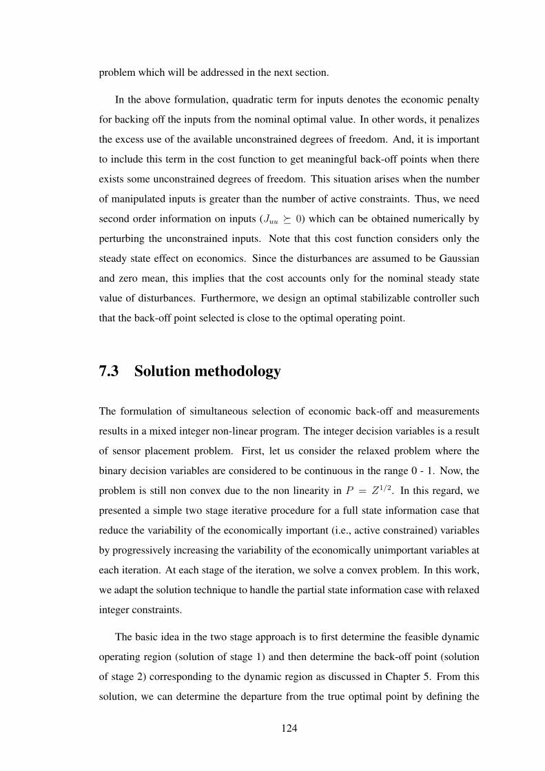
problem which will be addressed in the next section.

In the above formulation, quadratic term for inputs denotes the economic penalty

for backing off the inputs from the nominal optimal value. In other words, it penalizes

the excess use of the available unconstrained degrees of freedom. And, it is important

to include this term in the cost function to get meaningful back-off points when there

exists some unconstrained degrees of freedom. This situation arises when the number

of manipulated inputs is greater than the number of active constraints. Thus, we need

second order information on inputs (Juu � 0) which can be obtained numerically by

perturbing the unconstrained inputs. Note that this cost function considers only the

steady state effect on economics. Since the disturbances are assumed to be Gaussian

and zero mean, this implies that the cost accounts only for the nominal steady state

value of disturbances. Furthermore, we design an optimal stabilizable controller such

that the back-off point selected is close to the optimal operating point.

7.3 Solution methodology

The formulation of simultaneous selection of economic back-off and measurements

results in a mixed integer non-linear program. The integer decision variables is a result

of sensor placement problem. First, let us consider the relaxed problem where the

binary decision variables are considered to be continuous in the range 0 - 1. Now, the

problem is still non convex due to the non linearity in P = Z1/2. In this regard, we

presented a simple two stage iterative procedure for a full state information case that

reduce the variability of the economically important (i.e., active constrained) variables

by progressively increasing the variability of the economically unimportant variables at

each iteration. At each stage of the iteration, we solve a convex problem. In this work,

we adapt the solution technique to handle the partial state information case with relaxed

integer constraints.

The basic idea in the two stage approach is to first determine the feasible dynamic

operating region (solution of stage 1) and then determine the back-off point (solution

of stage 2) corresponding to the dynamic region as discussed in Chapter 5. From this

solution, we can determine the departure from the true optimal point by defining the

124

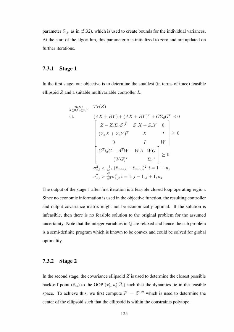
parameter δi,j , as in (5.32), which is used to create bounds for the individual variances.

At the start of the algorithm, this parameter δ is initialized to zero and are updated on

further iterations.

7.3.1 Stage 1

In the first stage, our objective is to determine the smallest (in terms of trace) feasible

ellipsoid Z and a suitable multivariable controller L.

minX�0,Σz�0,Y

Tr(Z)

s.t. (AX +BY ) + (AX +BY )T +GΣdGT ≺ 0

Z − ZdΣdZdT ZxX + ZuY 0

(ZxX + ZuY )T X I

0 I W

� 0

CTQC − ATW −WA WG

(WG)T Σ−1d

� 0

σ2z,i <

14α2 (zmax,i − zmin,i)2; i = 1 · · ·nz

σ2z,i >

δ2i,jα2 σ

2z,j; i = 1, j − 1, j + 1, nz

The output of the stage 1 after first iteration is a feasible closed loop operating region.

Since no economic information is used in the objective function, the resulting controller

and output covariance matrix might not be economically optimal. If the solution is

infeasible, then there is no feasible solution to the original problem for the assumed

uncertainty. Note that the integer variables in Q are relaxed and hence the sub problem

is a semi-definite program which is known to be convex and could be solved for global

optimality.

7.3.2 Stage 2

In the second stage, the covariance ellipsoid Z is used to determine the closest possible

back-off point (zss) to the OOP (x∗0, u∗0, d0) such that the dynamics lie in the feasible

space. To achieve this, we first compute P = Z1/2 which is used to determine the

center of the ellipsoid such that the ellipsoid is within the constraints polytope.

125

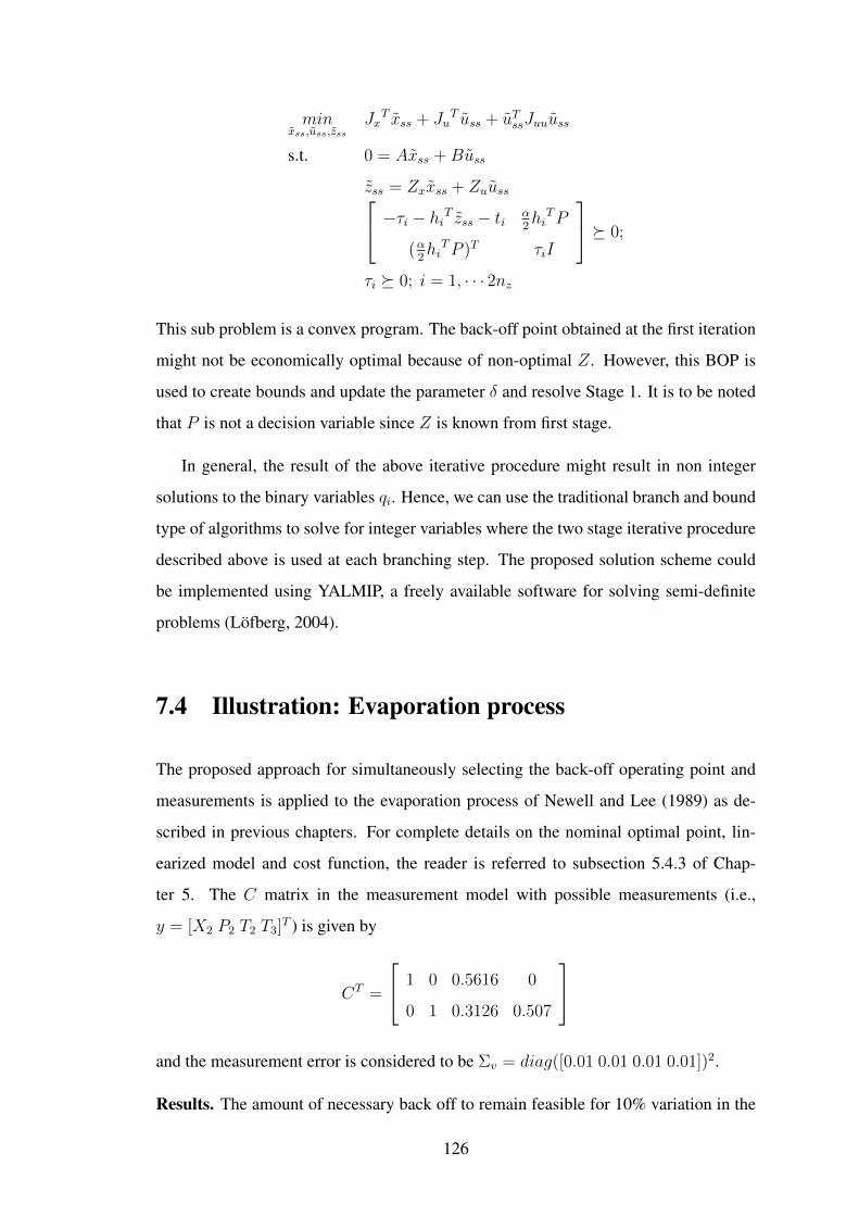
minxss,uss,zss

JxT xss + Ju

T uss + uTssJuuuss

s.t. 0 = Axss +Buss

zss = Zxxss + Zuuss −τi − hiT zss − ti α2hiTP

(α2hiTP )T τiI

� 0;

τi � 0; i = 1, · · · 2nz

This sub problem is a convex program. The back-off point obtained at the first iteration

might not be economically optimal because of non-optimal Z. However, this BOP is

used to create bounds and update the parameter δ and resolve Stage 1. It is to be noted

that P is not a decision variable since Z is known from first stage.

In general, the result of the above iterative procedure might result in non integer

solutions to the binary variables qi. Hence, we can use the traditional branch and bound

type of algorithms to solve for integer variables where the two stage iterative procedure

described above is used at each branching step. The proposed solution scheme could

be implemented using YALMIP, a freely available software for solving semi-definite

problems (Löfberg, 2004).

7.4 Illustration: Evaporation process

The proposed approach for simultaneously selecting the back-off operating point and

measurements is applied to the evaporation process of Newell and Lee (1989) as de-

scribed in previous chapters. For complete details on the nominal optimal point, lin-

earized model and cost function, the reader is referred to subsection 5.4.3 of Chap-

ter 5. The C matrix in the measurement model with possible measurements (i.e.,

y = [X2 P2 T2 T3]T ) is given by

CT =

1 0 0.5616 0

0 1 0.3126 0.507

and the measurement error is considered to be Σv = diag([0.01 0.01 0.01 0.01])2.

Results. The amount of necessary back off to remain feasible for 10% variation in the

126

35 35.5 36 36.5 37 37.540

45

50

55

60

65

70

75

80

Product composition, X2 (%)

Ope

ratin

g pr

essu

re, P

2 (kP

a)

Figure 7.1: Product composition vs operating pressure. a) Continuous line : FSI caseb) Dashed line : PSI case

35 35.5 36 36.5 37 37.5

0

10

20

30

40

50

60

70

80

90

100

Product composition, X2 (%)

Rec

ircu

latio

n fl

ow r

ate,

F3

(kg/

min

)

Figure 7.2: Product composition vs recirculation flow rate

35 35.5 36 36.5 37 37.5240

260

280

300

320

340

360

380

400

Product composition, X2 (%)

Stea

m p

ress

ure,

P10

0 (kP

a)

Figure 7.3: Product composition vs steam pressure

127

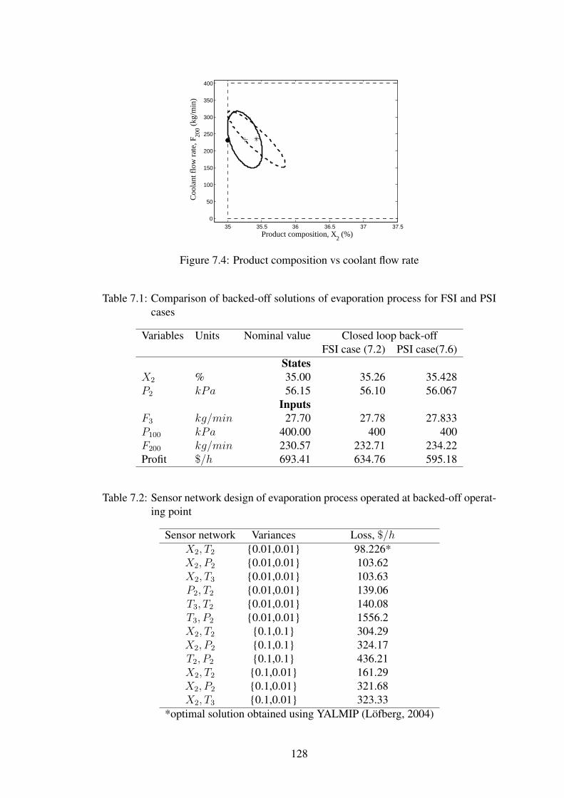
35 35.5 36 36.5 37 37.50

50

100

150

200

250

300

350

400

Product composition, X2 (%)

Coo

lant

flo

w r

ate,

F20

0 (kg

/min

)

Figure 7.4: Product composition vs coolant flow rate

Table 7.1: Comparison of backed-off solutions of evaporation process for FSI and PSIcases

Variables Units Nominal value Closed loop back-offFSI case (7.2) PSI case(7.6)

StatesX2 % 35.00 35.26 35.428P2 kPa 56.15 56.10 56.067

InputsF3 kg/min 27.70 27.78 27.833P100 kPa 400.00 400 400F200 kg/min 230.57 232.71 234.22Profit $/h 693.41 634.76 595.18

Table 7.2: Sensor network design of evaporation process operated at backed-off operat-ing point

Sensor network Variances Loss, $/hX2, T2 {0.01,0.01} 98.226*X2, P2 {0.01,0.01} 103.62X2, T3 {0.01,0.01} 103.63P2, T2 {0.01,0.01} 139.06T3, T2 {0.01,0.01} 140.08T3, P2 {0.01,0.01} 1556.2X2, T2 {0.1,0.1} 304.29X2, P2 {0.1,0.1} 324.17T2, P2 {0.1,0.1} 436.21X2, T2 {0.1,0.01} 161.29X2, P2 {0.1,0.01} 321.68X2, T3 {0.1,0.01} 323.33

*optimal solution obtained using YALMIP (Löfberg, 2004)

128

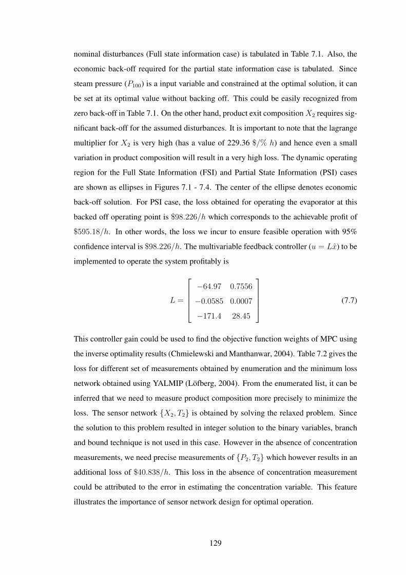
nominal disturbances (Full state information case) is tabulated in Table 7.1. Also, the

economic back-off required for the partial state information case is tabulated. Since

steam pressure (P100) is a input variable and constrained at the optimal solution, it can

be set at its optimal value without backing off. This could be easily recognized from

zero back-off in Table 7.1. On the other hand, product exit compositionX2 requires sig-

nificant back-off for the assumed disturbances. It is important to note that the lagrange

multiplier for X2 is very high (has a value of 229.36 $/% h) and hence even a small

variation in product composition will result in a very high loss. The dynamic operating

region for the Full State Information (FSI) and Partial State Information (PSI) cases

are shown as ellipses in Figures 7.1 - 7.4. The center of the ellipse denotes economic

back-off solution. For PSI case, the loss obtained for operating the evaporator at this

backed off operating point is $98.226/h which corresponds to the achievable profit of

$595.18/h. In other words, the loss we incur to ensure feasible operation with 95%

confidence interval is $98.226/h. The multivariable feedback controller (u = Lx) to be

implemented to operate the system profitably is

L =

−64.97 0.7556

−0.0585 0.0007

−171.4 28.45

(7.7)

This controller gain could be used to find the objective function weights of MPC using

the inverse optimality results (Chmielewski and Manthanwar, 2004). Table 7.2 gives the

loss for different set of measurements obtained by enumeration and the minimum loss

network obtained using YALMIP (Löfberg, 2004). From the enumerated list, it can be

inferred that we need to measure product composition more precisely to minimize the

loss. The sensor network {X2, T2} is obtained by solving the relaxed problem. Since

the solution to this problem resulted in integer solution to the binary variables, branch

and bound technique is not used in this case. However in the absence of concentration

measurements, we need precise measurements of {P2, T2} which however results in an

additional loss of $40.838/h. This loss in the absence of concentration measurement

could be attributed to the error in estimating the concentration variable. This feature

illustrates the importance of sensor network design for optimal operation.

129

7.5 Summary

In this chapter, we addressed the economic back-off operating point selection prob-

lem for partial state information case where both disturbances and measurement errors

are considered as uncertainties. The formulation also yields a multivariable controller

which when implemented to operate the evaporation process at the determined eco-

nomic back-off operating point will ensure feasible and profitable operation. Further-

more, we obtained the optimal set of measurements from the formulation that result in

minimal loss.

130

CHAPTER 8

CONCLUSIONS AND RECOMMENDATIONS

8.1 Conclusions

In this thesis, we demonstrated that the selection of sensors, set points, and controller

parameters significantly affect the economic performance of the process plant. It is

important to understand the nature of optimal solution (constrained or unconstrained),

available unconstrained degrees of freedom, and disturbance charactersitics, while mak-

ing the structural and parametric decisions to improve profitability.

The sensor network obtained using the conventional design procedures leads to

poor economic performance as demonstrated in ammonia and evaporator case studies.

Therefore, the proposed average loss based sensor network design formulation will be a

useful tool for designers, as the loss function directly quantifies the potential economic

benefit one would achieve using the resulting sensor network. In addition, the explicit

availability of analytical expression for the average loss function, can be a ready-to-

use tool while retrofitting the existing network, to quickly screen alternatives. This

profit based formulation is an important step towards obtaining sensor networks us-

ing commensurable metrics, within the integrated optimization and control framework.

The proposed average loss formulation can be used to select sensors that will improve

the economic performance, only if we have some unconstraint degrees of freedom to

optimize. Therefore, if there are no unconstrained degrees of freedom, measurement

selection does not affect optimal operation critically, and we can select measurements

using conventional sensor network formulations. Also, the average loss based sensor

network design formulation proposed in Chapter 3 can be seen as the generalization

of the one presented in Chapter 2, where identical weighting is given to all process

variables of interest. More importantly, the optimization formulations of the sensor

selection problem resulting from integer relaxation are convex. Therefore, the main

benefits of MICP approach is two-fold: (1) efficient solvers for solving MICP problems

are currently available, and (2) the resulting optimal solution is globally optimal. Since

the overall estimation error of the sensor network should also be as minimal as possible

for better control, the lexicographic approach presents the elegant way to combine both

the objectives. Furthermore, the problem was extended to find the sensor network that

was robust to sensor failures while retaining the above mentioned benefits. This was

accomplished by selecting redundant measurements such that all sub-networks were

observable. In all the relevant problems studied, the original MICP nature of the sensor

selection problem is preserved, and hence guaranteeing globally optimal solutions.

In the set point selection problem, we considered the case when the nominal steady

state solution is at the intersection of constraints. Since the constrained steady state

optimal point results in operational difficulties, back-off approach is often identified

as an important tool for practitioners to avoid infeasibility issues. Also, the back-off

directly quantifies the static economic performance one would achieve if operated at

the backed-off point. Therefore, the proposed the economic back-off approach will be

an useful scientific tool for operators to find the new operating point in the presence

of white noise type disturbances. For this purpose, a novel two-stage iterative solution

procedure was proposed.Additionally, the proposed method determines the best linear

multivariable controller to be employed to achieve the dynamic economic performance.

In other words, the potential economic benefit one could achieve by reducing the level

of back-off with the help of linear multivariable controller was discussed. At the con-

strained optimal point, if there exists some unconstrained degrees of freedom, then it

is important to use quadratic approximation of the cost to obtain meaningful back-off

values. Further, we extended the economic back-off approach by additionally consider-

ing the presence of measurements errors. In this case, the level of back-off is due to the

contribution of both the uncertainties. Therefore, to conclude, the optimal controller

design can reduce the level of back-off caused because of disturbances and a suitable

sensor network selection can reduce the level of back-off contribution caused by mea-

surement errors. Finally, the actual economic performance of the designed controller

was compared with an equivalent MPC controller.

132

8.2 Recommendations

The following list briefly describes some of the possible research directions.

• A systematic procedure on how to make the rational choice on the parametricand structural decisions in the context of optimal operation was presented. Thisframework should be extended to include non-linear models, model uncertainties,etc.

• The use of branch and bound technique in the measurement selection problemlimits the applicability of the proposed MICP approach to moderately sized inte-ger decision variables. Therefore, a computationally efficient technique for largescale systems will be of great use in making the optimal decision. One probableapproach could be to find tight SDP or SOC relaxations of the integer restric-tions instead of the linear relaxations used here. This will result in better boundvalues that could possibly require lesser number of branching and hence can sub-stantially decrease the computational burden for large scale systems. Anotherapproach could be to solve the integer relaxed problem by adding an appropriatepenalty term to the cost function for not being closer to the integer values. In thisregard, the sum of the weighted `1 norm could be a possible penalty function.

• The MICP approach presented for sensor selection is based on the linear (or lin-earized) model of the process. The approach can be extended for bilinear sys-tems, which typically has linear models for mass balances (involving flow vari-ables only) and bilinear models for species balances (involving bilinear terms offlow and composition variables) and energy balances in some cases (involvingbilinear terms of flow and temperature variables). In this case, the sensor selec-tion problem can be solved sequentially in two steps: first, decide on the flowmeasurements using the linear model involving flow variables only and second,assuming all flows are estimable which makes the species and energy balanceslinear, use the proposed MICP approach to decide on the remaining number ofsensors for obtaining better estimate of the temperature or composition variables.This decoupling enables one to solve two sensor selection problems of smallersize. However, such an approach may not result in globally optimal sensor net-work though the sub-problems are solved to global optimality.

• The network properties such as observability, redundancy and estimability are in-corporated in the current MICP approach. However, there exist no SDP or SOCrepresentation for reliability of the sensor network. Obtaining such a representa-tion will allow the reliability based sensor selection problem to be casted withinthe framework of conic optimization.

• The sensor selection presented in this thesis for sensor failure situations assumesequal sensor failure probability for all the sensors. Extension to unequal sensorfailure probability case will be more useful and general.

• Since sensor failures are considered as different scenarios, the number of LMIs tobe added also increase by a factor of n in case of single sensor failure. For mul-tiple sensor failures, the number of LMIs to be added will grow exponentially,

133

therefore a better approximation is required even for a moderately sized problem.One approach could be to consider each sensor failure as different scenarios andfit an ellipsoidal representation that contains all the scenarios and solve the robustversion of the problem with ellipsoidal uncertainty. This might result in computa-tionally tractable robust formulation. Otherwise, scenario optimization approachbased on radomization of the observability constraints might be possible.

• For constrained processes which give rise to feasibility issues in the presence ofdisturbances, the optimal back-off approach was presented for Gaussian whitenoise type disturbances. A systematic approach for a more general class of dis-turbances will be useful.

• In this work, we presented a novel two-stage solution technique for solving anon-convex problem which arises in back-off studies. Theoretical properties ofthe proposed algorithm need to be investigated and its applicability to a wide classof non-convex optimization problems can be studied.

• Design variables play a significant role in the optimal operation. Therefore, op-timal design studies that could result in flexible operation under uncertain condi-tions for nominally constrained processes is a possible research direction.

• The proposed economic back-off approach is based on fixed set of active con-straints. However, in some cases the set of active constraints might change de-pending on the disturbance magnitude. New methods have to be developed forachieving profitable and flexible operation in the face of changing active con-straints.

134

APPENDIX A

DERIVATION OF Equation 2.13

Recall that the process model has been expressed in terms of the primary variables zp.

The true state variables of the process z are related to true primary variables as follows:

z = Czp (A.1)

and the measurement equation is now expressed as:

y = Czp + v (A.2)

The reconciled estimates zp and z satisfy the following:

zp = (CTQC)−1CTQy (A.3)

z = Czp (A.4)

Let us derive the expressions for the expected values:

E(y) = E(Czp + v) = Czp (A.5)

E(yyT ) = E(Czp + v)(Czp + v)T = CzpzTp C

T +Q−1 (A.6)

as v is zero mean with covariance Q−1

E(z) = C(CTQC)−1CTQE(y) = C(CTQC)−1CTQCzp = Czp (A.7)

The error covariance of the reconciled estimates is defined as:

Σz = E((z − z)(z − z)T ) = zzT − 2zE(zT ) + E(zzT ) (A.8)

The first two terms in the above is simply −CzpzTp CT . Let us evaluate the last term:

E(zzT ) = E((C(CTQC)−1CTQy)(C(CTQC)−1CTQy)T ) (A.9)

= C(CTQC)−1CTQE(yyT )QC(CTQC)−1CT (A.10)

= C(CTQC)−1CTQ(CzpzTp C

T +Q−1)QC(CTQC)−1CT (A.11)

= CzpzTp C

T + C(CTQC)−1CT (A.12)

Thus, the error covariance of the estimates is:

Σz = −CzpzTp CT + CzpzTp C

T + C(CTQC)−1CT (A.13)

= C(CTQC)−1CT (A.14)

136

REFERENCES

1. Ahmed, S. K. and D. J. Chmielewski, On the tuning of predictive controllers for hybridfuel cell vehicle applications. In 10th IFAC International Symposium on Dynamics andControl of Process Systems,. 2013, 129–134.

2. Ali, Y. (1993). Sensor Network Design for Maximizing Reliability of Chemical Pro-cesses. Ph.D. thesis, IIT Kanpur, India.

3. Ali, Y. and S. Narasimhan (1993). Sensor network design for maximizing reliabilityof linear processes. AIChE Journal, 39(5), 820–828.

4. Ali, Y. and S. Narasimhan (1995). Redundant sensor network design for linear pro-cesses. AIChE Journal, 41(10), 2237–2249.

5. Ali, Y. and S. Narasimhan (1996). Sensor network design for maximizing reliabilityof bilinear processes. AIChE Journal, 42(9), 2563–2575.

6. Alizadeh, F. and D. Goldfarb (2003). Second-order cone programming. Mathematicalprogramming, 95(1), 3–51.

7. Alstad, V., S. Skogestad, and E. S. Hori (2009). Optimal measurement combinationsas controlled variables. Journal of Process Control, 19(1), 138 – 148.

8. Amrit, R., J. B. Rawlings, and D. Angeli (2011). Economic optimization using modelpredictive control with a terminal cost. Annual Reviews in Control, 35(2), 178 – 186.

9. Angeli, D., R. Amrit, and J. Rawlings (2012). On average performance and stabilityof economic model predictive control. IEEE Transactions on Automatic Control, 57(7),1615–1626.

10. Anjos, M. and J. Lasserre, Introduction to Semidefinite, Conic and Polynomial Opti-mization, volume 166 of International Series in Operations Research & ManagementScience. Springer US, 2012.

11. Aske, E. M. (2009). Design of plantwide control systems with focus on maximizingthroughput. Ph.D. thesis, Norwegian University of Science and Technology, Trond-heim, Norway.

12. Aske, E. M. B., S. Strand, and S. Skogestad (2008). Coordinator MPC for maximizingplant throughput. Computers & Chemical Engineering, 32, 195 – 204.

13. Bagajewicz, M. and E. Cabrera (2002). New MILP formulation for instrumentationnetwork design and upgrade. AIChE Journal, 48(10), 2271–2282.

14. Bagajewicz, M., M. Markowski, and A. Budek (2005). Economic value of precisionin the monitoring of linear systems. AIChE Journal, 51(4), 1304 – 1309.

138

15. Bagajewicz, M. and M. Sánchez (2000). Cost-optimal design of reliable sensor net-works. Computers & Chemical Engineering, 23(11-12), 1757 – 1762.

16. Bagajewicz, M. J. (1997). Design and retrofit of sensor networks in process plants.AIChE Journal, 43(9), 2300–2306.

17. Bagajewicz, M. J. and M. C. Sánchez (1999). Design and upgrade of nonredundantand redundant linear sensor networks. AIChE Journal, 45(9), 1927–1938.

18. Bahri, P., J. Bandoni, G. Barton, and J. Romagnoli (1995). Back-off calculationsin optimising control: A dynamic approach. Computers & Chemical Engineering, 19,Supplement 1(0), 699 – 708.

19. Bahri, P., J. Bandoni, and J. Romagnoli (1996). Effect of disturbances in optimizingcontrol: steady state open loop backoff problem. AIChE Journal, 42(4), 983–994.

20. Betta, G. and A. Pietrosanto, Instrument fault detection and isolation: State of theart and new research trends. In IEEE Conference Proceedings on Instrumentation andMeasurement Technology Conference, volume 1. 1998, 483–489.

21. Bhushan, M., S. Narasimhan, and R. Rengaswamy (2008). Robust sensor networkdesign for fault diagnosis. Computers & Chemical Engineering, 32, 1067 – 1084.

22. Bhushan, M. and R. Rengaswamy (2000). Design of sensor network based on thesigned directed graph of the process for efficient fault diagnosis. Industrial & Engi-neering Chemistry Research, 39(4), 999–1019.

23. Bhushan, M. and R. Rengaswamy (2002a). Comprehensive design of a sensor net-work for chemical plants based on various diagnosability and reliability criteria. 1.Framework. Industrial & Engineering Chemistry Research, 41(7), 1826–1839.

24. Bhushan, M. and R. Rengaswamy (2002b). Comprehensive design of a sensor net-work for chemical plants based on various diagnosability and reliability criteria. 2.Applications. Industrial & Engineering Chemistry Research, 41(7), 1840–1860.

25. Biegler, L. T., A survey on sensitivity-based nonlinear model predictive control. In10th IFAC International Symposium on Dynamics and Control of Process Systems,.2013, 499–510.

26. Boyd, S. and L. Vandenberghe, Convex Optimization. Cambridge University Press,New York, USA, 2004.

27. Carnero, M. C., J. L. Hernández, and M. C. Sánchez, Optimal sensor network de-sign and upgrade using tabu search. In L. Puigjaner and A. Espuña (eds.), EuropeanSymposium on Computer-Aided Process Engineering-15, 38th European Symposium ofthe Working Party on Computer Aided Process Engineering, volume 20 of ComputerAided Chemical Engineering. Elsevier, 2005, 1447 – 1452.

28. Chmielewski, D. J. and A. M. Manthanwar (2004). On the tuning of predictive con-trollers: Inverse optimality and the minimum variance covariance constrained controlproblem. Industrial & Engineering Chemistry Research, 43(24), 7807–7814.

139

29. Chmielewski, D. J., T. Palmer, and V. Manousiouthakis (2002). On the theory ofoptimal sensor placement. AIChE Journal, 48(5), 1001–1012.

30. Davis, J., Report from NSF workshop on Smart Process Manufacturing.2008. URL https://smart-process-manufacturing.ucla.edu/presentations-and-reports/spm-operations-technology-road-map/SPMroadmapsectionv5_1.pdf/at_download/file.

31. de Hennin, S., J. Perkins, and G. Barton, Structural decisions in on-line optimization.In Proceedings of PSE ‘94. Kyongju, Korea, 1994, 297–302.

32. Diehl, M., R. Amrit, and J. Rawlings (2011). A lyapunov function for economicoptimizing model predictive control. IEEE Transactions on Automatic Control, 56(3),703–707.

33. Engell, S. (2007). Feedback control for optimal process operation. Journal of ProcessControl, 17(3), 203 – 219. Special Issue {ADCHEM} 2006 Symposium.

34. Figueroa, J., P. Bahri, J. Bandoni, and J. Romagnoli (1996). Economic impact ofdisturbances and uncertain parameters in chemical processes: A dynamic back-off anal-ysis. Computers & Chemical Engineering, 20(4), 453 – 461.

35. Forbes, J., T. Marlin, and J. MacGregor (1994). Model adequacy requirements foroptimizing plant operations. Computers & Chemical Engineering, 18(6), 497 – 510.An International Journal of Computer Applications in Chemical Engineering.

36. Fraleigh, L. M., M. Guay, and J. F. Forbes (2003). Sensor selection for model-basedreal-time optimization: Relating design of experiments and design cost. Journal ofProcess Control, 13(7), 667 – 678.

37. Frank, P. M. (1990). Fault diagnosis in dynamic systems using analytical andknowledge-based redundancy: A survey and some new results. Automatica, 26(3),459 – 474.

38. Govatsmark, M. S. and S. Skogestad (2005). Selection of controlled variables androbust setpoints. Industrial & Engineering Chemistry Research, 44(7), 2207–2217.

39. Grant, M. and S. Boyd (2011). CVX: MATLAB software for disciplined convex pro-gramming, version 1.21. URL http://cvxr.com/cvx.

40. Halvorsen, I. J., S. Skogestad, J. C. Morud, and V. Alstad (2003). Optimal selectionof controlled variables. Industrial & Engineering Chemistry Research, 42(14), 3273–3284.

41. Heath, J. A., I. K. Kookos, and J. D. Perkins (2000). Process control structure selec-tion based on economics. AIChE Journal, 46(10), 1998–2016.

42. Joshi, S. and S. Boyd (2009). Sensor selection via convex optimization. IEEE Trans-actions on Signal Processing, 57(2), 451 –462.

43. Kariwala, V. and Y. Cao (2010). Bidirectional branch and bound for controlled variableselection part III: Local average loss minimization. IEEE Transactions on IndustrialInformatics, 6(1), 54 –61.

140

44. Kariwala, V., Y. Cao, and S. Janardhanan (2008). Local self-optimizing control withaverage loss minimization. ndustrial & Engineering Chemistry Research, 47(4), 1150–1158.

45. Kookos, I. K. (2005). Real-time regulatory control structure selection based on eco-nomics. Industrial & Engineering Chemistry Research, 44(11), 3993–4000.

46. Kookos, I. K. and J. D. Perkins (2002). An algorithmic method for the selection ofmultivariable process control structures. Journal of Process Control, 12(1), 85 – 99.

47. Kotecha, P., M. Bhushan, R. Gudi, and M. Keshari (2008). A duality based frame-work for integrating reliability and precision for sensor network design. Journal ofProcess Control, 18, 189 – 201.

48. Kretsovalis, A. and R. S. Mah (1987). Effect of redundancy on estimation accuracy inprocess data reconciliation. Chemical Engineering Science, 42(9), 2115 – 2121.

49. Lai, C.-A., C.-T. Chang, C.-L. Ko, and C.-L. Chen (2003). Optimal sensor place-ment and maintenance strategies for mass-flow networks. Industrial & EngineeringChemistry Research, 42(19), 4366–4375.

50. Loeblein, C. and J. Perkins (1998). Economic analysis of different structures of on-line process optimization systems. Computers & Chemical Engineering, 22(9), 1257 –1269.

51. Loeblein, C. and J. D. Perkins (1999a). Structural design for on-line process optimiza-tion: I. dynamic economics of mpc. AIChE Journal, 45(5), 1018–1029.

52. Loeblein, C. and J. D. Perkins (1999b). Structural design for on-line process optimiza-tion: Ii. application to a simulated fcc. AIChE Journal, 45(5), 1030–1040.

53. Löfberg, J., YALMIP : A toolbox for modeling and optimization in MATLAB. InProceedings of the CACSD Conference. Taipei, Taiwan, 2004.

54. Maciejowski, J., Predictive Control: With Constraints. Prentice Hall, 2002.

55. Mazzour, E. H., D. Hodouin, and S. Makni (2003). Optimal sensor implementation inmetallurgical plants–an application to a generic mineral separation plant. InternationalJournal of Mineral Processing, 69(1-4), 185 – 203.

56. Menon, G., M. Nabil, and S. Narasimhan, Branch and bound algorithm for optimalsensor network design. In 10th IFAC International Symposium on Dynamics and Con-trol of Process Systems,. 2013, 690–695.

57. Modén, P. E. and M. Lundh, Performance monitoring for model predictive controlmaintenance. In European Control Conference (ECC). 2013, 3770 – 3775.

58. Mohideen, M. J., J. D. Perkins, and E. N. Pistikopoulos (1996). Optimal design ofdynamic systems under uncertainty. AIChE Journal, 42(8), 2251–2272.

59. Morari, M., Y. Arkun, and G. Stephanopoulos (1980). Studies in the synthesis ofcontrol structures for chemical processes: Part i: Formulation of the problem. processdecomposition and the classification of the control tasks. analysis of the optimizingcontrol structures. AIChE Journal, 26(2), 220–232.

141

60. Narasimhan, S. and C. Jordache, Data reconciliation & gross error detection: anintelligent use of process data. Gulf Publishing Co., Houston, TX, USA, 2000.

61. Narasimhan, S. and R. Rengaswamy (2007). Quantification of performance of sensornetworks for fault diagnosis. AIChE Journal, 53(4), 902–917.

62. Narraway, L., J. Perkins, and G. Barton (1991). Interaction between process de-sign and process control: Economic analysis of process dynamics. Journal of ProcessControl, 1(5), 243 – 250.

63. Narraway, L. T. and J. D. Perkins (1993). Selection of process control structure basedon linear dynamic economics. Industrial & Engineering Chemistry Research, 32(11),2681–2692.

64. Newell, R. B. and P. Lee, Applied process control : a case study. Prentice Hall : NewYork, 1989.

65. Nguyen, D. T. and M. J. Bagajewicz (2009). On the impact of sensor maintenance poli-cies on stochastic-based accuracy. Computers & Chemical Engineering, 33(9), 1491 –1498.

66. Nocedal, J. and S. J. Wright, Numerical Optimization. Springer Series in OperationsResearch. Springer, 2006.

67. Peng, J. and D. Chmielewski, Optimal sensor network design using the minimallybacked-off operating point notion of profit. In American control conference. 2005, 220– 224.

68. Peng, J.-K., A. M. Manthanwar, and D. J. Chmielewski (2005). On the tuning ofpredictive controllers: The minimum back-off operating point selection problem. Ind.& Eng. Chem. Res., 44(20), 7814–7822.

69. Perkins, J., Interaction between process design and process control. In IFAC sympo-sium on DYCORD+ ‘89. Netherlands, 1989, 349–357.

70. Perkins, J., C. Gannavarapu, and G. Barton, Choosing control structures based oneconomics. In Internation symposium on control for profit. Newcastle, 1989, 1–12.

71. Qin, S. and T. A. Badgwell (2003). A survey of industrial model predictive controltechnology. Control Engineering Practice, 11(7), 733 – 764.

72. Raghuraj, R., M. Bhushan, and R. Rengaswamy (1999). Locating sensors in complexchemical plants based on fault diagnostic observability criteria. AIChE Journal, 45, 310– 322.

73. Rao, C. V. and J. B. Rawlings (1999). Steady states and constraints in model predictivecontrol. AIChE Journal, 45(6), 1266–1278.

74. Rawlings, J., D. Angeli, and C. Bates, Fundamentals of economic model predictivecontrol. In 2012 IEEE 51st Annual Conference on Decision and Control (CDC). 2012,3851–3861.

142

75. Rawlings, J., D. Bonne, J. Jorgensen, A. Venkat, and S. Jorgensen (2008). Unreach-able setpoints in model predictive control. IEEE Transactions on Automatic Control,53(9), 2209–2215.

76. Rawlings, J. B. and D. Q. Mayne, Model Predictive Control : Theory and Design.Madison, Wis. Nob Hill Pub. cop., 2009.

77. Roberts, P. (1979). Algorithm for steady-state system optimization and parameter es-timation. International Journal of Systems Science, 10(7), 719–734.

78. Sánchez, M. C. and M. J. Bagajewicz (2000). On the impact of corrective maintenancein the design of sensor networks. Industrial & Engineering Chemistry Research, 39(4),977–981.

79. Scokaert, P. O. M. and J. B. Rawlings (1999). Feasibility issues in linear modelpredictive control. AIChE Journal, 45(8), 1649–1659.

80. Sen, S., S. Narasimhan, and K. Deb (1998). Sensor network design of linear processesusing genetic algorithms. Computers & Chemical Engineering, 22(3), 385 – 390.

81. Sherali, H. D. (1982). Equivalent weights for lexicographic multi-objective programs:Characterizations and computations. European Journal of Operational Research, 11(4),367 – 379.

82. Skogestad, S. (2000). Self-optimizing control: the missing link between steady-stateoptimization and control. Computers & Chemical Engineering, 24(2 - 7), 569 – 575.

83. Skogestad, S., Economic Plantwide Control. John Wiley & Sons Ltd, Malaysia, 2012,229–251.

84. Vandenberghe, L. and S. Boyd (1996). Semidefinite programming. SIAM review,38(1), 49–95.

85. Young, J., C. Swartz, and R. Ross (1996). On the effects of constraints, economicsand uncertain disturbances on dynamic operability assessment. Computers & ChemicalEngineering, 20, Supplement 1(0), S677 – S682.

143

LIST OF PAPERS BASED ON THESIS

Journal publications

1. M. Nabil and Sridharakumar Narasimhan. Sensor Network Design for OptimalProcess Operation Based on Data Reconciliation. Ind. Eng. Chem. Res., 51 (19),6789 – 6797, 2012.

2. M. Nabil, Sridharakumar Narasimhan and Sigurd Skogestad. Profitable and dy-namically feasible operating point selection for constrained processes. Journalof Process Control, 24 (5), 531–541, 2014.

3. M. Nabil, Sridharakumar Narasimhan and Sigurd Skogestad. Economic perfor-mance of Model Predictive Control for constrained processes. Manuscript underpreparation.

Publications in conference proceedings

1. Presented titled Design of Optimal Sensor Network based on Economic Objec-tives at the AIChE Annual Meeting 2010. Salt Lake City, US, Nov. 7-12, 2010.

2. Presented titled Economic back-off selection based on optimal multivariable con-troller at the 8th IFAC symposium on Advanced Control of Chemical Pro-cesses (ADCHEM 2012). Singapore, July 10-13, 2012.

3. Presented titled Integrated Sensor Network Design at the 11th InternationalSymposium on Process Systems Engineering (PSE2012). Singapore, July 15-19, 2012.

4. Presented titled Optimal selection of sensor network and backed-off operatingpoint based on economics at the 12th European Control Conference (ECC 13).Zurich, Switzerland, July 17-19, 2013.

144