Optimal Scalable Video Multiplexing in Optimal Scalable Video Multiplexing in

Mobile Broadcast NetworksMobile Broadcast Networks

Farid M. Tabrizi, Cheng-Hsin Hsu,

Mohamed Hefeeda, and Joseph G. Peters

Network Systems Lab, Simon Fraser University, Canada

Deutsche Telekom Lab, USA

OutlineOutline

Motivations

Mobile Video Broadcast Networks

Problem Statement and Formulation

Our Solution

Evaluation Results

Conclusions

2

MotivationsMotivations

3

Mobile videos are getting increasingly popular

However, delivering mobile videos over unicast

channels of cellular networks is inefficient

- Analysis predicted that 3G cellular networks would collapse

with only 40% mobile phone users watching 8-minute video

each day [Liang et al. PTC’08]

- AT&T is phasing out their unlimited data plans

More efficient delivery method is needed

We study broadcast networks that support

multicast/broadcast for higher spectrum efficiency

Mobile Broadcast Networks Mobile Broadcast Networks

4

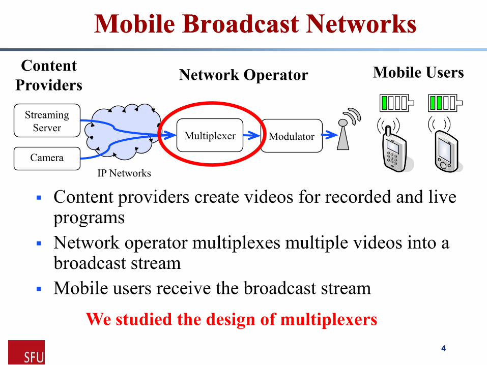
Streaming

Server

Camera

Multiplexer Modulator

IP Networks

Content

ProvidersNetwork Operator Mobile Users

We studied the design of multiplexers

Content providers create videos for recorded and live programs

Network operator multiplexes multiple videos into a broadcast stream

Mobile users receive the broadcast stream

ChallengesChallenges

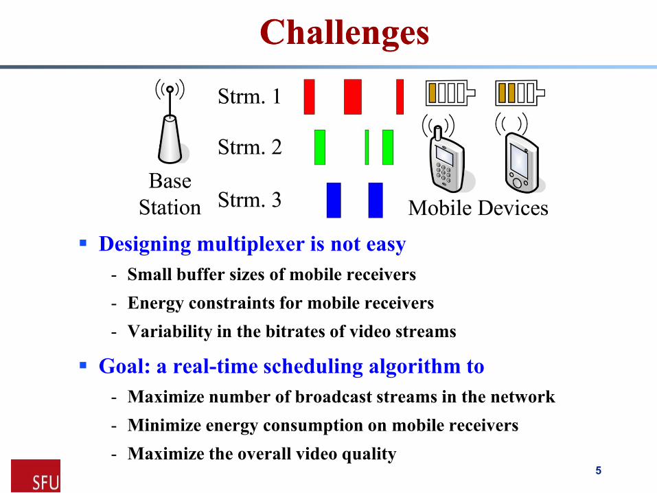
Designing multiplexer is not easy

- Small buffer sizes of mobile receivers

- Energy constraints for mobile receivers

- Variability in the bitrates of video streams

Goal: a real-time scheduling algorithm to

- Maximize number of broadcast streams in the network

- Minimize energy consumption on mobile receivers

- Maximize the overall video quality5

MediumMedium--Grained Scalable StreamsGrained Scalable Streams

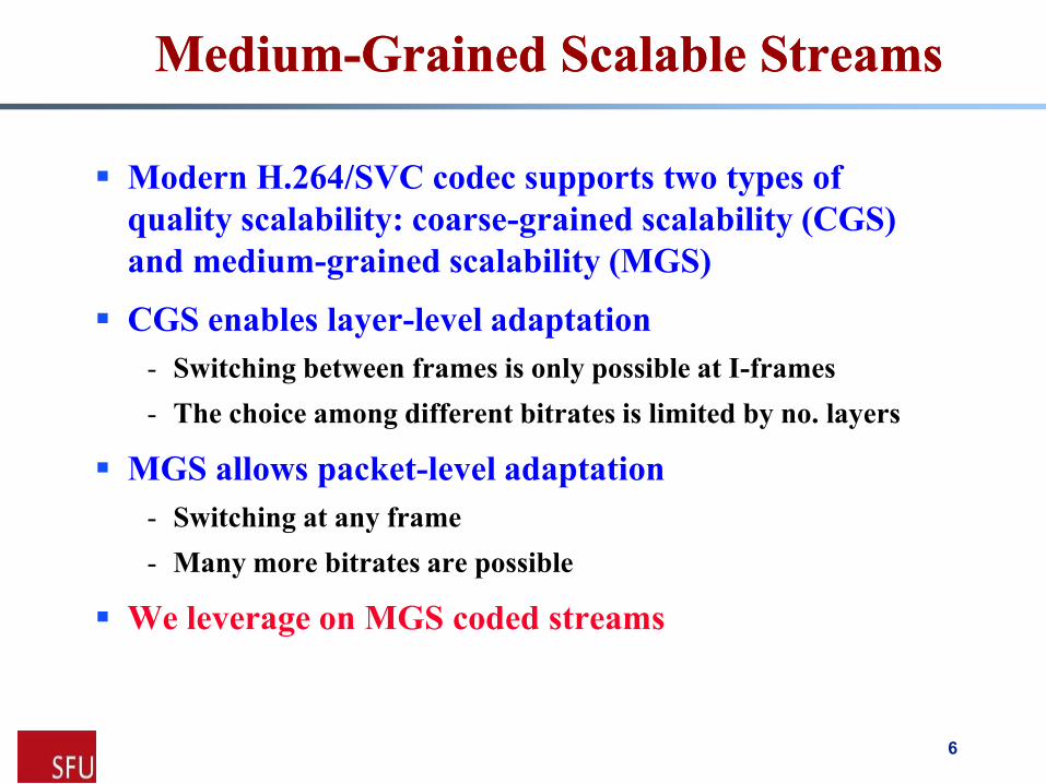
Modern H.264/SVC codec supports two types of

quality scalability: coarse-grained scalability (CGS)

and medium-grained scalability (MGS)

CGS enables layer-level adaptation

- Switching between frames is only possible at I-frames

- The choice among different bitrates is limited by no. layers

MGS allows packet-level adaptation

- Switching at any frame

- Many more bitrates are possible

We leverage on MGS coded streams

6

Problem StatementProblem Statement

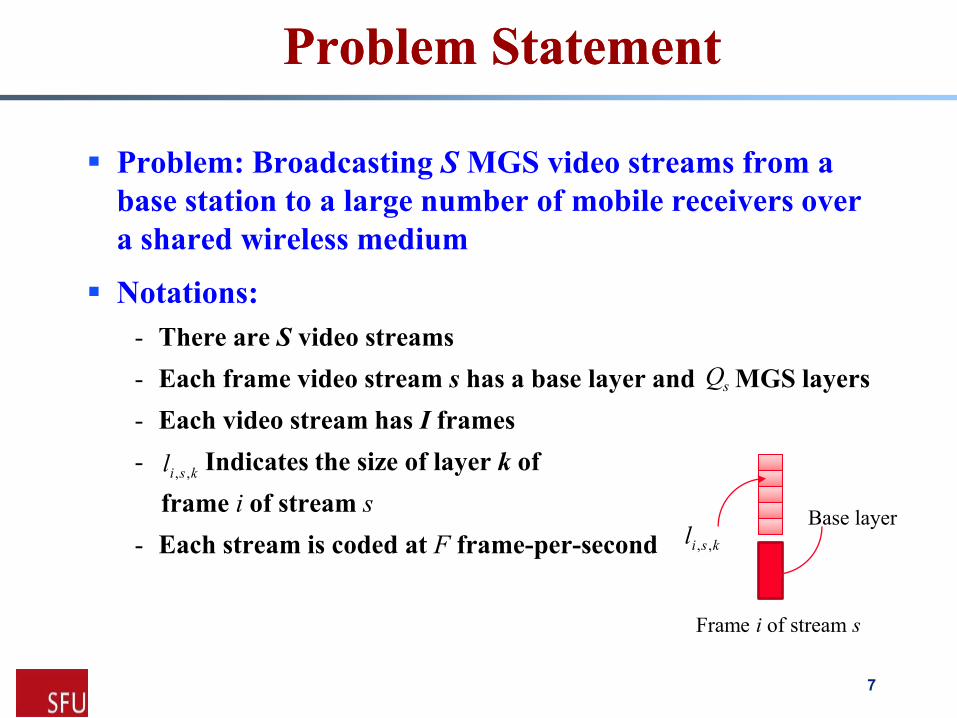
Problem: Broadcasting S MGS video streams from a

base station to a large number of mobile receivers over

a shared wireless medium

Notations:

- There are S video streams

- Each frame video stream s has a base layer and MGS layers

- Each video stream has I frames

- Indicates the size of layer k of

frame i of stream s

- Each stream is coded at F frame-per-second

sQ

ksil ,,

ksil ,,

Frame i of stream s

Base layer

7

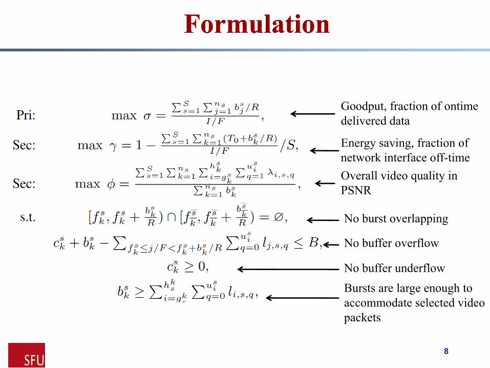
FormulationFormulation

Goodput, fraction of ontime

delivered data

Energy saving, fraction of

network interface off-time

Overall video quality in

PSNR

No burst overlapping

No buffer overflow

No buffer underflow

Bursts are large enough to

accommodate selected video

packets

8

Problem SolutionProblem Solution

Split receiver buffer of size B to two buffers of size B/2

For each video stream, we assign time windows

At each time window of each video stream, one buffer

is being drained while the other buffer is being filled

Earliest-deadline-first scheduling in each window

When the draining buffer is empty, we switch the

buffers

If due to bandwidth limitations a complete video

cannot be sent, we drop MGS layers in a rate-

distortion optimized manner and schedule a burst for

the empty buffer

9

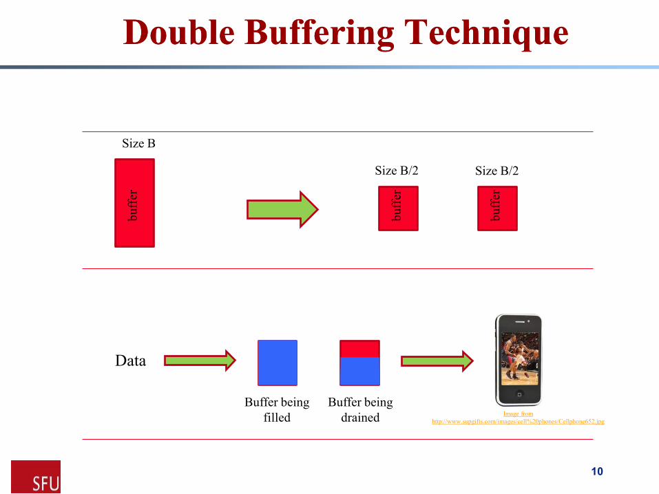
Double Buffering TechniqueDouble Buffering Technique

bu

ffer

bu

ffer

bu

ffer

Buffer being

drained

Buffer being

filled

Data

Size B

Size B/2 Size B/2

Image from

http://www.supgifts.com/images/cell%20phones/Cellphone652.jpg

10

Evaluation SetupEvaluation Setup

Use a MobileTV testbed developed in our lab

- The base station: a Linux box with RF signal modulator

implementing the physical layer of mobile broadcast protocol

- Indoor antenna to transmit DVB-H compliant signals

Settings

- We set the modulator to use 16-QAM (Quadrature Amplitude

Modulation)

- 10MHz radio channel

- Transition overhead time To=100 ms

11

Evaluation Setup (cont.)Evaluation Setup (cont.)

Video streams

- 10 video streams of different categories of: sport, TV

game show, documentary, talk show and have very

different visual characteristics

- Bitrates ranging from 250 to 768 kbps

- We created video streams with different MGS layers and

the trace file for each stream using JSVM

Comparison

- We compare our OSVM algorithm with MBS (Mobile

Broadcast Solution) from Nokia and SMS algorithm [MM’09] which has been previously developed in our Lab

12

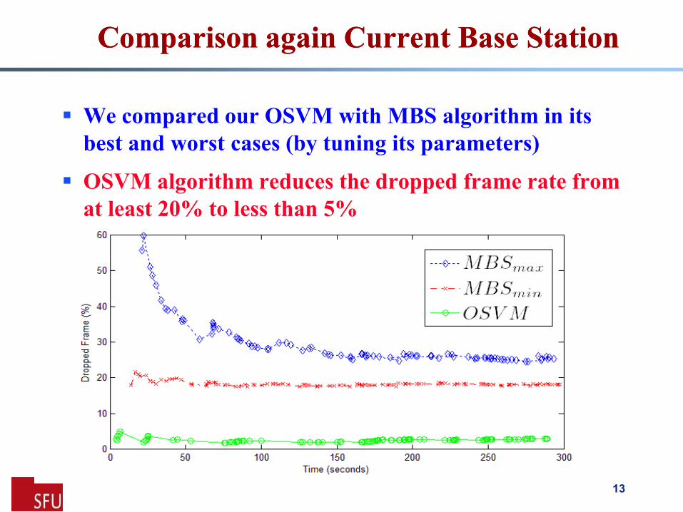
Comparison again Current Base StationComparison again Current Base Station

We compared our OSVM with MBS algorithm in its

best and worst cases (by tuning its parameters)

OSVM algorithm reduces the dropped frame rate from

at least 20% to less than 5%

13

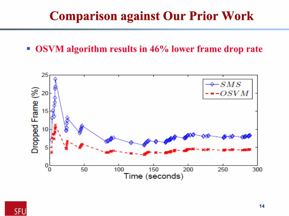
Comparison against Our Prior WorkComparison against Our Prior Work

OSVM algorithm results in 46% lower frame drop rate

14

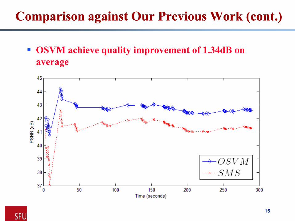
Comparison against Our Previous Work (cont.)Comparison against Our Previous Work (cont.)

OSVM achieve quality improvement of 1.34dB on

average

15

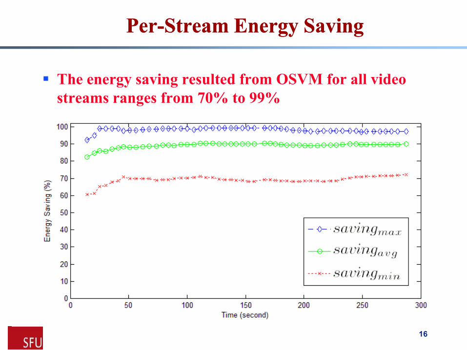
PerPer--Stream Energy SavingStream Energy Saving

The energy saving resulted from OSVM for all video

streams ranges from 70% to 99%

16

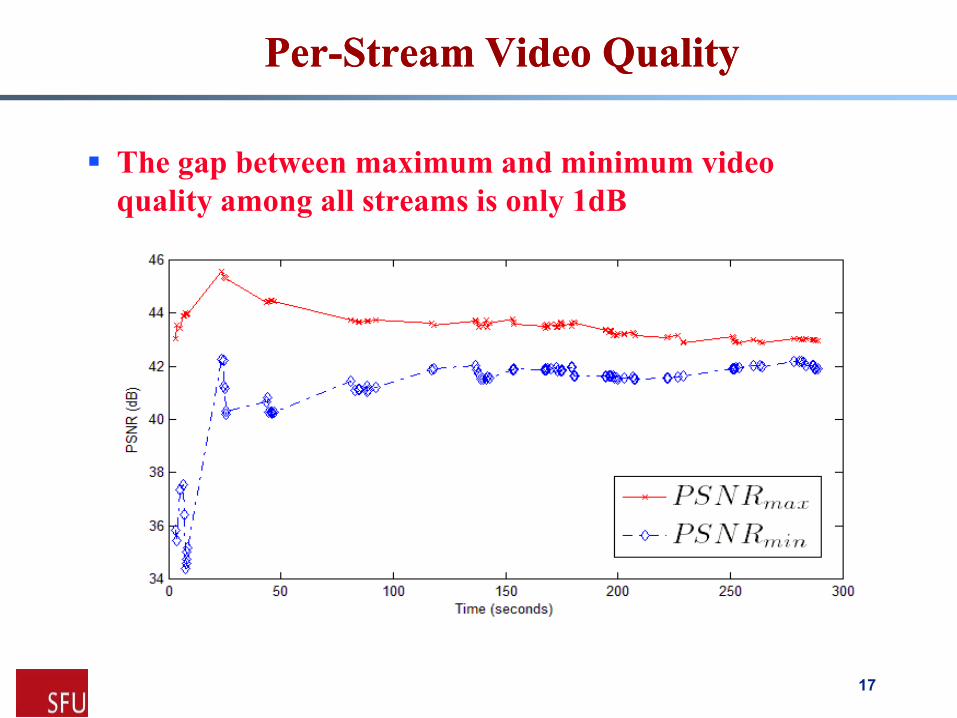
PerPer--Stream Video Quality Stream Video Quality

The gap between maximum and minimum video

quality among all streams is only 1dB

17

ConclusionsConclusions

We studied scalable video broadcast networks

We formulated a burst scheduling problem to jointly

optimize: (i) video quality, (ii) network goodput, and

(iii) receiver energy consumption.

We proposed an efficient algorithm for the problem

We implement the proposed algorithm in a real mobile

TV testbed

Extensive experimental results indicate that our

algorithm outperforms the algorithms used in current

base stations and proposed in our previous work [MM’09]

18

Thank You

19

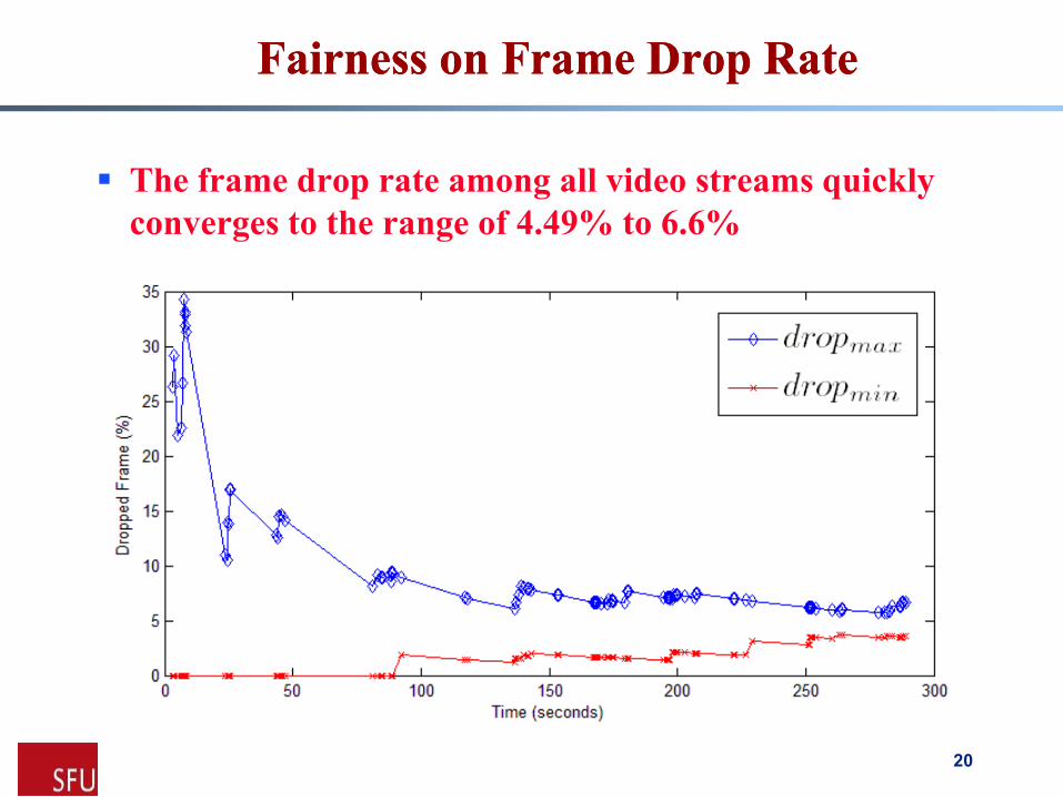
Fairness on Frame Drop RateFairness on Frame Drop Rate

The frame drop rate among all video streams quickly

converges to the range of 4.49% to 6.6%

20

Future WorkFuture Work

Making the solution adaptive based on the changes in

bitrate of video streams

Considering the effect of larger lookahead window on

the performance of multiplexing algorithm

Using other scalability opportunities like temporal

scalability

21

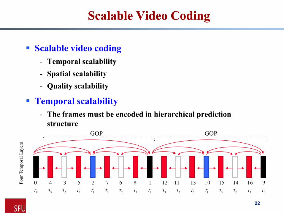
Scalable Video CodingScalable Video Coding

Scalable video coding

- Temporal scalability

- Spatial scalability

- Quality scalability

Temporal scalability

- The frames must be encoded in hierarchical prediction

structure

GOP GOP

0 4 3 5 2 7 6 8 1 12 11 13 10 15 14 16 9

0T 3T2T 3T

1T 3T2T 3T 0T 3T

2T 3T1T 3T

2T 3T 0T

Four

Tem

pora

l L

ayer

s

22

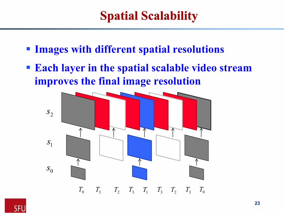
Spatial ScalabilitySpatial Scalability

Images with different spatial resolutions

Each layer in the spatial scalable video stream

improves the final image resolution

0s

1s

2s

0T3T 2T 3T

1T 3T 2T 3T 0T

23

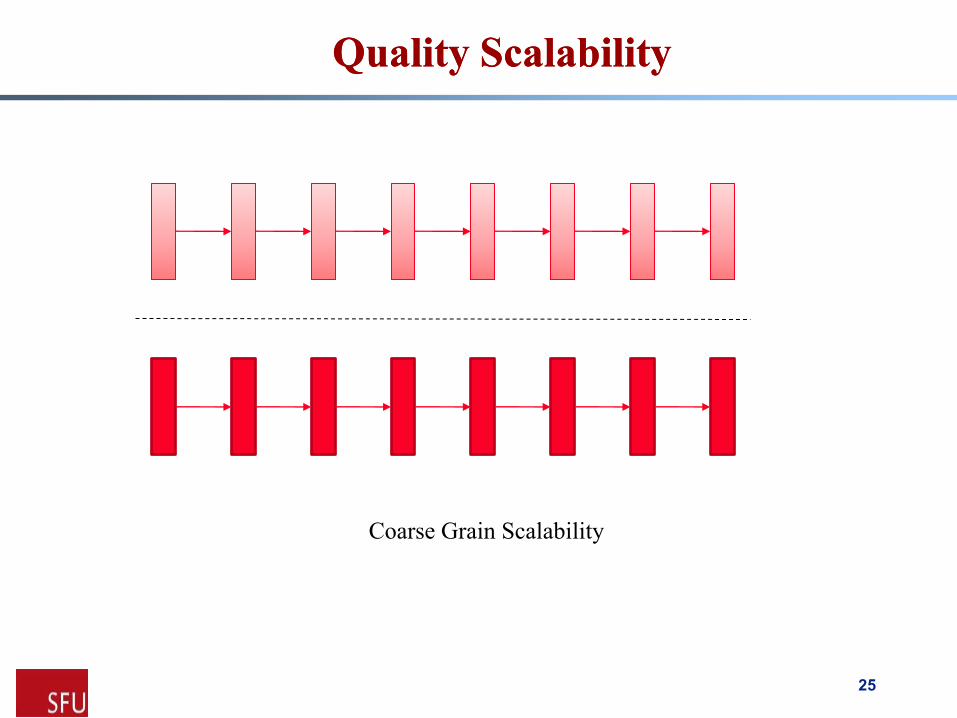
Quality ScalabilityQuality Scalability

Quality scalability could be considered as a special case

of spatial scalability

Dividing the video into several quality layers: Coarse

Grain Scalability (CGS)

- In CGS, motion estimation is conducted in each spatial layer

separately

• Switching between frames is only possible at I-frames

• The choice among different bitrates is limited to the

number of layers

24

Quality ScalabilityQuality Scalability

Coarse Grain Scalability

25

Quality ScalabilityQuality Scalability

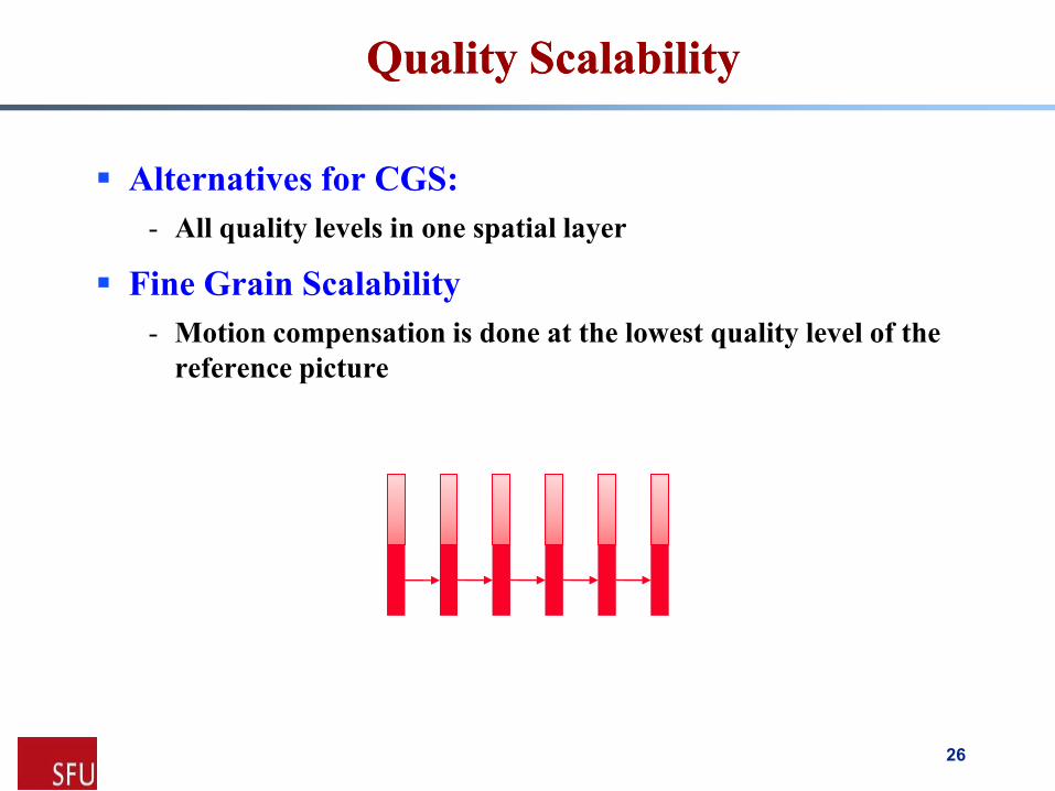
Alternatives for CGS:

- All quality levels in one spatial layer

Fine Grain Scalability

- Motion compensation is done at the lowest quality level of the

reference picture

26

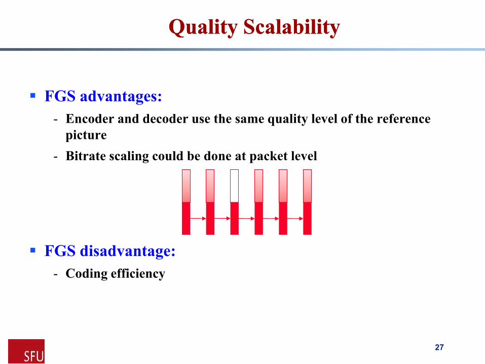
Quality ScalabilityQuality Scalability

FGS advantages:

- Encoder and decoder use the same quality level of the reference

picture

- Bitrate scaling could be done at packet level

FGS disadvantage:

- Coding efficiency

27

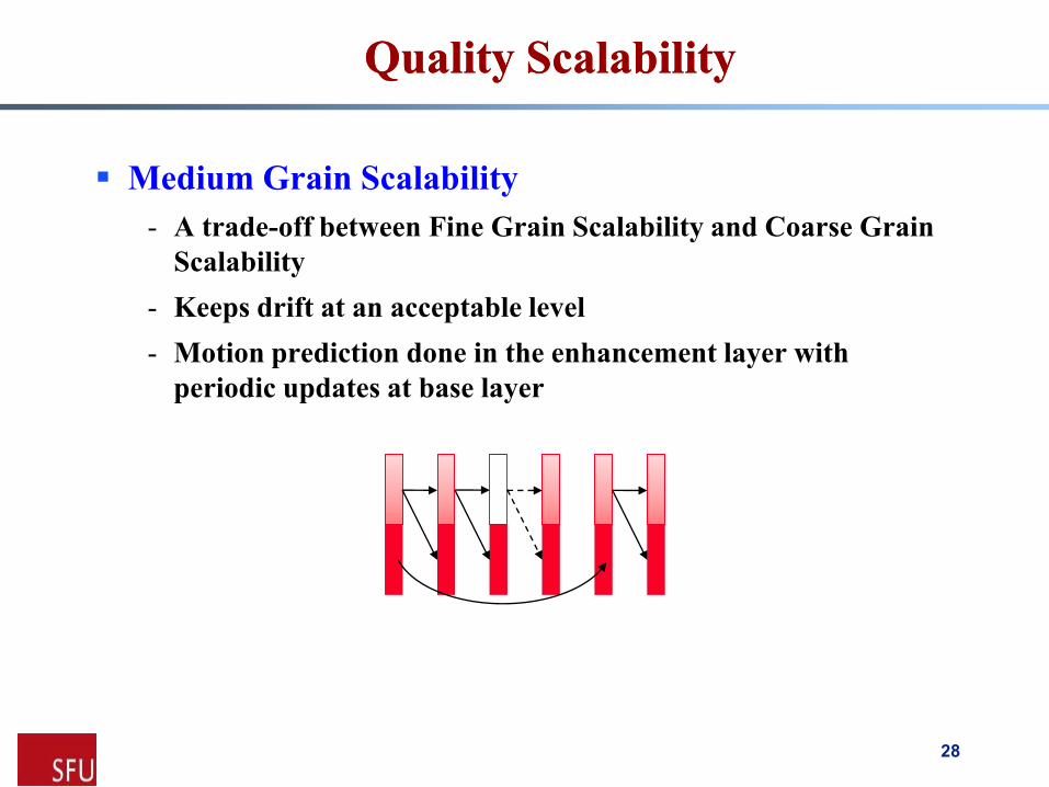
Quality ScalabilityQuality Scalability

Medium Grain Scalability

- A trade-off between Fine Grain Scalability and Coarse Grain

Scalability

- Keeps drift at an acceptable level

- Motion prediction done in the enhancement layer with

periodic updates at base layer

28

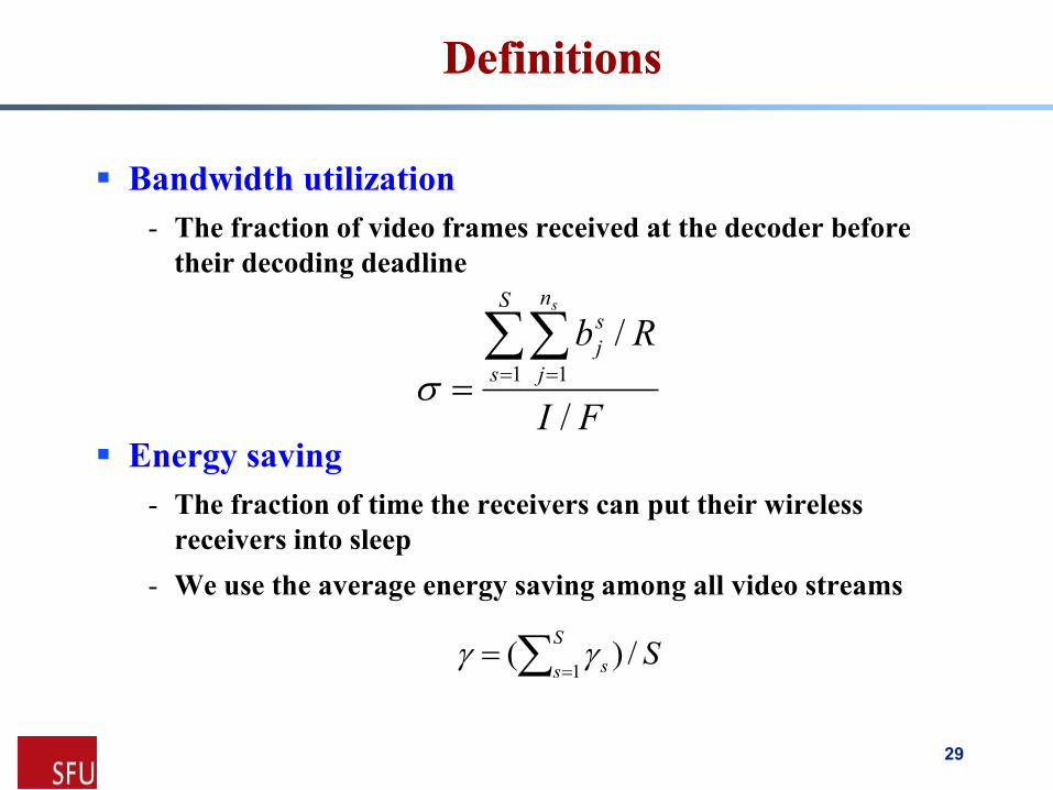
DefinitionsDefinitions

Bandwidth utilization

- The fraction of video frames received at the decoder before

their decoding deadline

Energy saving

- The fraction of time the receivers can put their wireless

receivers into sleep

- We use the average energy saving among all video streams

FI

RbS

s

n

j

s

j

s

/

/1 1

SS

s s /)(1

29

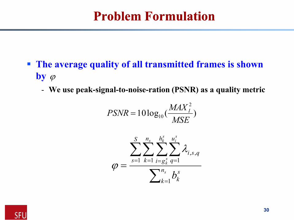
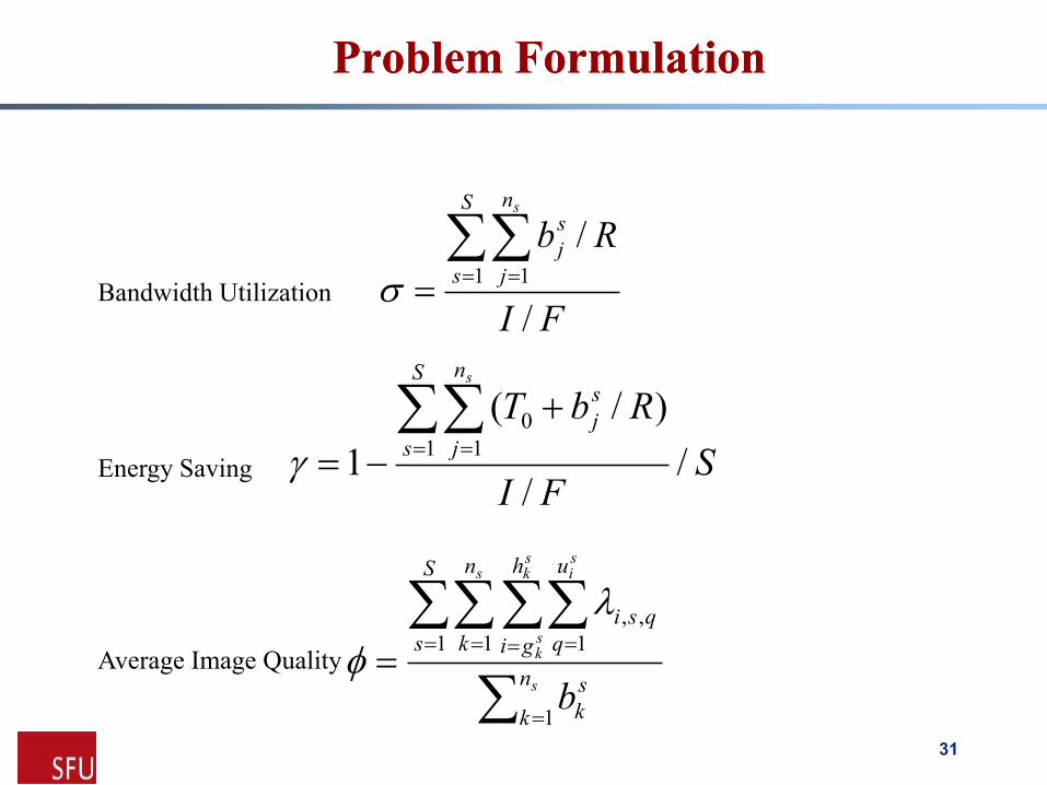
Problem FormulationProblem Formulation

The average quality of all transmitted frames is shown

by

- We use peak-signal-to-noise-ration (PSNR) as a quality metric

)(log102

10MSE

MAXPSNR I

s

ssk

sk

si

n

k

s

k

S

s

n

k

h

gi

u

q

qsi

b1

1 1 1

,,

30

Problem FormulationProblem Formulation

FI

RbS

s

n

j

s

j

s

/

/1 1

SFI

RbTS

s

n

j

s

j

s

//

)/(

11 1

0

s

ssk

sk

si

n

k

s

k

S

s

n

k

h

gi

u

q

qsi

b1

1 1 1

,,

Bandwidth Utilization

Energy Saving

Average Image Quality

31

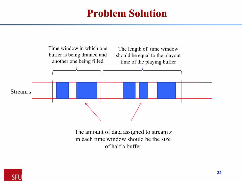
Problem SolutionProblem Solution

Time window in which one

buffer is being drained and

another one being filled

The amount of data assigned to stream s

in each time window should be the size

of half a buffer

The length of time window

should be equal to the playout

time of the playing buffer

Stream s

32

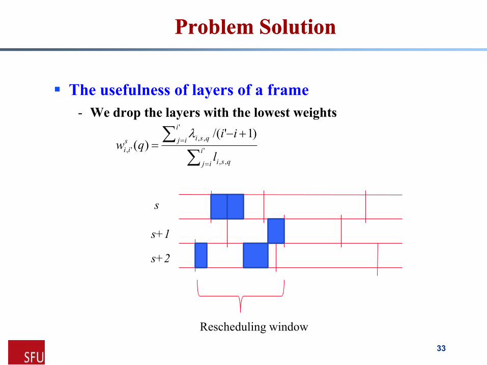
Problem SolutionProblem Solution

The usefulness of layers of a frame

- We drop the layers with the lowest weights

'

,,

'

,,

',

)1'/()(

i

ij qsi

i

ij qsis

ii

l

iiqw

s

s+1

s+2

Rescheduling window

33

Evaluation Setup (cont.)Evaluation Setup (cont.)

Video streams

- 10 video streams of different categories of: sport, TV game

show, documentary, talk show and have very different visual

characteristics

- Bitrates ranging from 250 to 768 kbps

- We created video streams with different MGS layers and the

trace file for each stream using “BitStreamExtractorStatic” tool

provided by JSVM

- We used “PSNRStatic” to determine the PSNR value of each

MGS layer of each video stream

Comparison

- We compare our OSVM algorithm with MBS (Mobile Broadcast

Solution) from Nokia and SMS algorithm [MM’09] which has been

previously developed in our Lab

34