Optimal resource allocation in a representative investor

Economic Modelling 50 (2015) 72–84

Contents lists available at ScienceDirect

Economic Modelling

j ourna l homepage: www.e lsev ie r .com/ locate /ecmod

Optimal resource allocation in a representative investor economy☆

Orlando Gomes ⁎Lisbon Accounting and Business School (ISCAL/IPL), Business Research Unit, (UNIDE/ISCTE-IUL), Portugal

☆ I acknowledge the insightful and helpful comments othe journal's editor. The usual disclaimer applies. I also thBusiness Research Unit of the Lisbon University InstituUI0315/2011).⁎ Lisbon Accounting and Business School (ISCAL/IPL), A

035 Lisbon, Portugal.E-mail address: [email protected].

http://dx.doi.org/10.1016/j.econmod.2015.06.0080264-9993/© 2015 Elsevier B.V. All rights reserved.

a b s t r a c t
a r t i c l e i n f o
Article history:Accepted 16 June 2015Available online 2 July 2015

Keywords:Representative investorAgency problemOptimal controlSaddle-path stabilityNeoclassical growth modelAK endogenous growth modelSentiment shocks

The Ramsey–Cass–Koopmans neoclassical growth setup and the AK endogenous growth framework are two pro-totypes of a class of growthmodelswhere, by assumption, investment resources are always perfectly allocated toproduction. As a corollary, these models offer a partial view of the growth process circumscribed to a limit case,namely the most favorable case in which all possible frictions on the allocation of investment resources are ab-sent. This paper adds to the conventional growth setup an optimal mechanism of assignment of investment re-sources that contemplates the possibility of inefficient allocation. In the assumed economy there is a singlerepresentative investor and a large number offirms that compete for the available resources. The new setuphigh-lights how agency costs may deviate the economy from the benchmark growth outcome, potentially generatingless desirable long-run results. The appeal of the proposed framework resides also on the fact that new determi-nants of growth emerge and take a leading role, namely the investor's sentiment and the quality of the firms' in-vestment proposals.

© 2015 Elsevier B.V. All rights reserved.

1. Introduction

Benchmark growth models offer a partial view on the process ofwealth creation. In such models, no friction on the allocation of invest-ment is present and, therefore, the economy tends to an upper limitoutcome of full efficiency. This paper devises and explores the dynamicsof a stylized optimal control problem concerning the intertemporalallocation of investment across firms in a market economy which,once merged with neoclassical and endogenous growth setups, allowsto gain a wider perspective on the growth process as approached bystandard theory in this field of knowledge.

The introduction of a mechanism inducing inefficiency on invest-ment allocation is relevant from an economic growth point of viewbecause it allows to depart from the implicit setting of full employmentof resources. Departures from potential output are now contemplated,and they will be determined by a multiplicity of factors, that mighteven include animal spirits under the form of the investor's sentiment.As one will realize, the new structure of analysis is much more amena-ble to the introduction of a discussion on the compatibility betweenbusiness cycles and growth than the conventional growth models.

The proposed setup involves a single representative investor whodecides, based on criteria established at the initial date, how to assign,

f an anonymous referee and ofank the financial support of thete (Grant code: PEst-OE/EGE/

v. Miguel Bombarda 20, 1069-

over time, a given amount of financial resources. Firms, that exist inthe economy in a potentially large number, will compete for thoseresources through the presentation to the investor of projects that detailthe activities they will engage on.

In the described setting, the investment allocation problem acquiresthe nature of an agency problem, where the representative investorplays the role of principal and the firms are the agents. Because theinvestor does not know with anticipation how the assigned budgetwill be employed by each firm, the criteria used to allocate it is thesignaling effort of each firm; firms communicate their financial needsto the investor through the presentation of projects that require re-sources to be prepared.

The allocation of funds involves a matching function between thequality of the mentioned project proposals and the funds that remainavailable to be attributed. This matching is such that both inputs areessential to obtain a positive outcome: at each specific time period, nofinancial transfer will occur if the firm under consideration does notpresent any investment project proposal; likewise, if no funds remainavailable, nomatter the quality of the proposed projects, the investmenttransfer will not take place. Furthermore, in the model's setting, itis considered that at each period the investor claims back fromevery firm a constant percentage of the previously allocated funds,e.g., under the form of contracted capital returns. This forces the firmsto systematically present new projects since, otherwise, they willprogressively lose the financial resources obtained in the past, andtheir funding will end up by falling to zero.

The investment allocation problem will be analyzed from the pointof view of thefirm. The firmwill want tomaximize, on an intertemporalperspective, the difference between the financial resources it is capable

http://crossmark.crossref.org/dialog/?doi=10.1016/j.econmod.2015.06.008&domain=pdf

http://dx.doi.org/10.1016/j.econmod.2015.06.008

mailto:[email protected]

http://dx.doi.org/10.1016/j.econmod.2015.06.008

http://www.sciencedirect.com/science/journal/02649993

73O. Gomes / Economic Modelling 50 (2015) 72–84

of obtaining and the costs it incurs to convince the investor about themerits of its investment plan. This optimization problemwill be subjectto a budget flow constraint, where the firm's assigned budget increaseswith the already mentioned matching process and diminishes with theautomatic withdrawal of funds at a constant rate.

Although simple in its structure, this is an analytically tractable modelthat delivers relevant insights on the process of investment allocation.Given the signaling costs, this model conducts to a result of inefficiency,in the sense that, in a long-term perspective, the aggregate allocated in-vestment will remain below 100%. A unique steady-state point is deter-mined and its position depends decisively on two entities: the quality oftheprojects presentedby thefirms and the overall sentiment of the inves-tor. As these forces shape the amount of aggregate investment, they willalso be main determinants of economic growth.

Project quality and investor sentiment are, according to the availableempirical evidence, two important drivers of the overall aggregateinvestment level and of the ability of the economies to generate addi-tional wealth. Section 2.2 briefly reviews some of the empirical litera-ture that highlights the key role that each of the two mentionedfeatures has in what concerns observed growth patterns. This evidenceis the key motivation for setting up the growth model in the sectionsthat follow. By placing investment in the forefront of the growth analy-sis one is able to realistically approach long-run wealth accumulation,without neglecting short-term fluctuations due to changes in the deter-minants of investment levels.

The remainder of the paper is organized as follows. In Section 2, areview of the relevant related literature is undertaken; this reviewcovers both theoretical contributions and empirical studies that high-light project quality and investor's sentiment as main drivers of thegrowthprocess. Section 3makes the analytical presentation of the prob-lem of the firm. Section 4 derives optimality conditions and discussesthe existence of the steady-state. In Section 5, the stability of the long-term equilibrium is investigated. Section 6 studies how eventualchanges on the values of exogenous variables, including the investor'ssentiment, might disturb transitional dynamics and the steady-state.In Section 7, the analytical framework of this paper is merged with theRamsey–Cass–Koopmans model in order to address the respective im-plications for growth, in a neoclassical perspective. Section 8 adaptsthe dynamic resource allocation problem to a setting of endogenousgrowth. Finally, Section 9 concludes.

2. Related literature

2.1. Theoretical foundations

The analysis in the following sections is inspired by a confluence ofdifferent strands of literature in economics. First, the financial literaturethat highlights agency relations and other sources of conflict betweeninvestors and investment recipients, which typically lead to investmentdistortions. Although the studies in turn of this subject tend to becircumscribed to a unique firm or group of integrated firms that under-take diversified activities, with themanagerswithin each department ordivision negotiating with the shareholders the correspondingbudget allocations, such discussion is straightforward to extrapolate toour environment of a unique representative investor in the economy.About agency and power relations within the firm, with consequenceson the allocation of scarce resources see, e.g., Shleifer and Vishny(1989), La Porta et al. (2000), Rajan et al. (2000), Burkart and Panunzi(2006), Agliardi and Agliardi (2008), Albuquerque and Wang (2008)and Chetty and Saez (2010).

The second relevant line of inquiry relates to the extensive literaturethat searches for an integrated analysis of growth and business cycles. Asignificant part of this literature takes conventional growth models andexplores the mechanisms that may induce persistent deviations ofvarying amplitude relatively to the full rational/full efficient benchmarkoutcome. One notorious contribution in this field is the work by Evans

et al. (1998), who identify the possibility of formation of two differentbalanced growth paths, one respecting to a state of low growth andthe other to a state of high growth. The economy may converge to oneor the other steady-state, depending on the agents' expectations.

Other work on growth cycles puts R&D investment at the center ofthe discussion. It is the case of Matsuyama (1999, 2001), Eriksson andLindh (2000), Walde (2002, 2005), Francois and Lloyd-Ellis (2003)and Shinagawa (2013). These studies emphasize the role of the cyclicalbehavior of the investment in innovation, in some cases triggeredby stochastic shocks and in other cases by endogenous processes, inshaping long-term cyclical growth.

The search for endemic causes of deterministic growth cycles has along tradition in economics, starting in the 1980s with the work ofBenhabib and Day (1981), Day (1982), Grandmont (1985) andDeneckere and Pelikan (1986), among others. Meaningful contributionson the field of endogenous growth cycles include Christiano andHarrison (1999), who proved the existence of chaos in a standarddeterministic version of the Real Business Cycles (RBC)model with pro-duction externalities, Brock and Hommes (1997, 1998), who encoun-tered rational routes to randomness in a setting of heterogeneousexpectations and discrete choice across distinct deliberation rules,Boldrin et al. (2001), who address the conditions under which endoge-nous growth models might generate endogenous cyclical motion,Gomes (2008), who considers that the non-rival nature of technologyconflicts with congestion externalities triggering in this way endoge-nous fluctuations, and Drugeon (2013), who highlights how a standardgrowth model with heterogeneous capital goods may conduct to a re-sult that departs from stability and give rise to competitive equilibriumgrowth cycles that are optimally generated.

In this article, growth cycles are not explicitly modeled, but theoffered framework creates the setting that allows to analyze their pres-ence. By conceiving an environment where optimal decisions by ratio-nal agents originate a less than efficient equilibrium result, in thesense that part of the investment resources will remain unemployed,one will be able to approach the conditions that lead to low or highgrowth (i.e., growth results that depart more or less from the fullefficiency benchmark outcome). If one allows for multiple investor'ssentiment states or systematic changes on the quality level of theprojects presented by firms to the investor, then one will be able to ap-proach cyclical motion in the presented growth framework.

A third strand of thought with relevance to the study in this paperconcerns the resurgence of animal spirits as a main determinant of theexplanation of short-run aggregate fluctuations. In a typical growthmodel, the entities capable of disturbing the generated balanced growthpath are technology, the preferences of consumers and other funda-mentals. RBC theory is built precisely on this assumption: systematicchanges on the technical conditions of production and other supplyside effects are, under this interpretation, the determinants of observedfluctuations (see King and Rebelo, 1999; Rebelo, 2005).

Alternative explanations, namely those that place the emphasis onagents' sentiments or animal spirits, have occasionally appeared in theliterature. Themost popular of these approaches is the one relatingmul-tiple equilibria and indeterminacy in optimal growth models. The inde-terminacy or sunspots literature, developed by Azariadis (1981), Cassand Shell (1983), Benhabib and Farmer (1994), Weder (2004) andGuerrazzi (2012), among others, supports that self-fulfilling propheciesleading to fluctuations might emerge in frictionless economies whenthe neoclassical model is modified in order to display multiple equilib-ria. Undermultiple equilibria, the beliefs of agents determine the trajec-tory to be followed from a series of optimal trajectories generated byeconomic fundamentals. Indeterminacy implies that there is not aunique optimal path to follow and, in this case, the trajectory that iseffectively followed depends on the self-fulfilling beliefs of the agents.

A revival of animal spirits as a centerpiece of the macroeconomicthought occurred with the publication of the book by Akerlof andShiller (2009), which coincided with the great recession of the end of

1 Although firms develop different tasks, we consider these to be perfect substitutesand, thus, a perfectly competitive market environment is considered. This assumption isuseful later on the paper, when addressing the impact of inefficient investment allocationover growth. Alternatively, a monopolistic competition setup could be taken, if the pro-ductive tasks developed by firms presented some degree of substitutability. This wouldimply considering a Dixit–Stiglitz production functionwhen presenting the growth frame-work, instead of the Cobb–Douglas function thatwill be assumed. There are nomeaningfuldifferences, in terms of the model's implications, of assuming one or the otherspecification.

74 O. Gomes / Economic Modelling 50 (2015) 72–84

thefirst decade of the twenty-first century. In the book, the view that in-dividual sentiments matter for economic outcomes was emphasized,leading to a new wave of interest on the impact of agents' sentimentsover economic results.

In the work that followed, two studies deserve to be highlighted.First, De Grauwe (2011), who claims that rational expectations andanimal spirits do not mix well and, thus, considers the presence of cog-nitive deficiencies in theway individuals process information. This doesnot mean that agents are irrational; instead, they are rational in under-standing that they have a limited capacity to interpret reality and, there-fore, have to use simple heuristics to take decisions. De Grauwe's modelgenerates endogenous waves of optimism and pessimism that might beassociated to the notion of animal spirits.

On a different plan, Angeletos and La'O (2013) propose a frameworkof analysis that combines market sentiments or animal spirits with theparadigm of rational expectations, as in the sunspots analysis. Differentlyfrom the sunspots setup, though, in the mentioned article multiple equi-libria are absent. The sentiments of agents emerge as the outcomeof com-munication constraints. The authors prove that if the communication israndom and decentralized, business cycles might arise in the context ofa typical neoclassical model, independently of shocks to fundamentals.It is the propagation of information that generates, in this case, endoge-nous fluctuations based on waves of optimism and pessimism.

In our article, there are evident departures relatively to the previouscontributions, but a relevant role is, in the same way, assigned to senti-ments, namely investor sentiments. Shocks on the confidence level ofthe representative investor will imply different rates of utilization ofthe resources available to generate value, implying potential fluctua-tions on the level of aggregate output.

In what concerns the particular modeling apparatus used in thispaper, it has antecedents on Gomes (2014, 2015), where inefficiencydue to agency relations is applied, respectively, to resource allocationin the brain and consequent cognitive decisions of the individual agent,and to a problem of budget setting within the divisions of a given firm.

2.2. A remark on the empirics of project quality and investor's sentiment

In the introduction, it was highlighted that the quality of investmentprojects and the investor's sentimentwill be themain drivers of growthin the analysis to pursue in the sections that follow. Besides this being anintuitive fact, there is also plenty evidence in the economics literaturepointing to the relevance of these elements as forces that decisivelyshape long-term growth trajectories.

Concerning project quality, one should start by noting that this is nota concept completely void of ambiguity. From a strictlyfinancial point ofview, the feasibility of a project is measured by its return in terms ofexpected cash-flows, but many other dimensions are relevant to assessinvestment quality from an economic growth point of view; the envi-ronmental impact or the expected society-wide externalities, positiveand negative, for instance, are two features that must be taken intoaccount as well.

Independently of the considered definition, the idea that the qualityof investment projects is a key determinant of growth finds in the empir-ical literature strong substantiation. This is, for instance, the result point-ed out by Sala-i-Martin and Artadi (2002), who have assessed thegrowth performance of Middle-East countries. The authors claim thatthe persistent low growth in this region of the globe is the direct conse-quence ofwrong or inefficient investment choices, which have their pro-found roots on several infra-structural deficiencies, namely the poorquality of institutions (financial, political, educational and others).

The discussion on the quality of investment projects is most of thetimes associated with, on one hand, public investment and, on the otherhand, foreign direct investment. Gupta et al. (2014) and O'Toole andTarp (2014) address the issue of public investment efficiency, mainly inthe perspective of the development of low-income economies. The men-tioned studies stress that measures of the adequacy of public investment

projects are a statistically significant variable when explaining growth indeveloping countries. Furthermore, public authorities should be con-cerned with suppressing rent-seeking behavior, bureaucracy and corrup-tion, since these are sources of inefficiency in the allocation of capital,leading to poor quality projects, and thus impair growth.

The notion of investment quality is also present on how the impactof capital flows from abroad is assessed. Alfaro and Charlton (2007)highlight the idea that some types of foreign direct investment are pref-erable than others; these authors associate the notion of foreign invest-ment quality to the effect that such investment has on growth in thehost country. In the same vein, Beckaert et al. (2011) demonstratethat the openness to capital flows from abroad typically enhancesinvestment efficiency and increases the quality of the investment pro-jects in the economy; and this is positively and strongly correlatedwith aggregate output growth.

A second strong claim in our analysis is that the investor's sentimentis a main driver of the aggregate investment flows that determine thepace of growth. This is documented, for instance, in the study by Arifand Lee (2014), who evaluate the relation between the sentiment ofinvestors, the expected equity returns and the level of aggregate invest-ment; not surprisingly, they conclude that periods when sentiments ofoptimism dominate are also periods in which the investment of firmsreaches the highest observable levels. Montone and Zwinkels (2015)also arrive to the conclusion that investor sentiments have real effects;specifically, these authors discuss the correlation between the senti-ment of capital owners and the growth of employment and output.

Another piece of evidence on the relation between investor confi-dence and growth is provided by Milani (2014), who estimates a mac-roeconomic general equilibrium model and finds evidence thatpsychological factors, namely those related to investment decisions,are a main determinant of the observable aggregate business cycles(they are responsible, according to this study, by more than 40% of theobservable business fluctuations, in the United States).

3. The dynamic resource allocation problem

Consider an economy populated by a single representative investorand a large number of firms, each one dedicated to the developmentof a specific productive task i ∈ N.1 Firms compete for the availableinvestment resources, which the representative investor allocates, ateach date t ≥ 0, after evaluating two criteria: (i) the signaling effort ofeach firm and (ii) the investment resources that remain available toassign.

Two arrays of endogenous variables play a role in themodel: the in-vestment shares allocated to the activities of each firm, ωi(t), and thecosts firms incur when presenting their projects to the capital holder,ϕi(t), which are alsomeasured as percentages of the available investor'sbudget. Variables ωi(t) and ϕi(t) correspond to non-negative values∀ t ≥ 0, and the respective aggregate levels cannot assume values largerthan the unity, i.e., Ω(t) ≡ ∫i ∈ N ωi(t)di ≤ 1 and Φ(t) ≡ ∫i ∈ N ϕi(t)di ≤ 1.

The objective of each firm is to maximize, in an intertemporal per-spective, the difference between the collected amount of investmentand the signaling costs associated with their acquisition. In this setting,variable ϕi(t) acquires the role of control variable, i.e., the firm is free tochoose howmuch it commits to acquire the funds thatwill serve the de-velopment of productive activities, in order to fulfill the referred

4 The optimality conditions hold under the presumption that the constraints over vari-ablesωi(t) ≥ 0, ϕi(t) ≥ 0, andΩ(t) ≤ 1,Φ(t) ≤ 1 are not violated. As the analytical study un-


objective. Under an infinite horizon and taking a constant in time dis-count rate, ρ N 0, the objective function of firm i is,2

Ui 0ð Þ ¼ Maxϕi tð Þ

Z þ∞

0ωi tð Þ−ϕi tð Þ½ �exp −ρtð Þdt; i ∈N: ð1Þ

A law of motion that is beyond the control of each firm will deter-mine the evolution over time of the assigned investment share, ωi(t);this is the state variable of the problem. Two processeswork in oppositedirections. The first process, through which the allocated investmentshare potentially increases, is generated by a matching function thatputs into confrontation the firm's signaling effort and the resourcesthe investor has left to be allocated at date t.

Definition 1. Matching function

Function fi[ϕi(t), 1 − Ω(t)] : ℝ+2 → ℝ+ is a matching function of the

firm's dynamic investment allocation problem if it obeys the followingproperties:

i) fi is a continuous and differentiable function;ii) fi is increasing in both arguments: ∂fi/∂ϕi N 0, ∂fi/∂(1− Ω) N 0;iii) fi is subject to decreasing marginal returns: ∂2fi/∂ϕi

2 b 0,∂2fi/∂(1− Ω)2 b 0;

iv) fi is homogeneous of degree 1: fi[ϵϕi(t), ϵ(1 − Ω(t))] =ϵfi[ϕi(t), 1 − Ω(t)], ∀ ϵ N 0;

v) Both inputs are essential for the matching process,fi[0, 1 − Ω(t)] = fi[ϕi(t), 0] = 0.

A possible explicit functional form for the matching function, thatobeys the above properties, is a Cobb–Douglas function of the type,

f i ϕi tð Þ;1−Ω tð Þ½ � ¼ B qiϕi tð Þ½ �β 1−Ω tð Þ½ �1−β; i ∈N;B N0; qiN0;β ∈ 0;1ð Þ:ð2Þ

Three parameters play a role in function (2); β is an elasticity param-eter, B is a measure of the investor's sentiment (a stronger positivesentiment implies a more efficient matching), and qi represents thequality of the projects firm i proposes to the investor. The qualityparameter is not necessarily of a same value across firms, meaningthat they are heterogeneous regarding the ability to convince the inves-tor infinancing the respective activities. Note that parameter qi emergesin the matching function as a weight over the signaling costs; thissignifies that the input of the matching function is not just the costincurred by the firm to communicate investment plans; the effective-ness of the communication is relevant as well.

The second force shaping the pace of the investment share respectsto an automatic withdrawal of resources by the investor, who claimsback, at each time period, a constant percentage of the attributedfunds. This allows the investor to continuously hold financial resourcesin search for the best investment opportunities, and compels firms, inorder to maintain or increase their budgets, to present, systematicallyover time, new projects to the investor. If no effort is made by thefirm to acquire resources, i.e., ifϕi(t)= 0, then the firmwill lose allocat-ed resources at a rate ζ ∈ (0, 1).

Under the specified conditions, the resource constraint takes theform3

ω�

i tð Þ ¼ f i ϕi tð Þ;1−Ω tð Þ½ �−ζωi tð Þ; i ∈N;ωi 0ð Þ ¼ ωi0 ∈ 0;1ð Þ given: ð3Þ

2 The discount rate indicates the degree of impatience of firm i concerning future netbudget allocation. A value of ρ close to zero implies a low level of impatience; if ρ is high,the future is heavily discounted and the agent is highly impatient. In order to simplify theanalysis, one considers that the discount rate is identical across firms.

3 Note that the model's formulation is purely deterministic and that perfect foresightholds for every assumed dynamic relation.

Definition 2. DRAP

The dynamic resource allocation problem (DRAP) faced by firm iconsists in solving Eq. (1) subject to Eq. (3) and to the constraints onvariables ωi(t) ≥ 0, ϕi(t) ≥ 0, and Ω(t) ≤ 1, Φ(t) ≤ 1.

4. Optimal solution and the steady-state

The solution of the DRAP will be a system of dynamic equationsreflecting the motion of the investment shares and of the respectiveco-state variable, pi(t) ≥ 0.

Proposition 1. The optimal solution of the DRAP, for the Cobb–Douglasmatching function, corresponds to the system of differential equations

ω�

i tð Þ ¼ B1= 1−βð Þ βqipi tð Þ½ �β= 1−βð Þ 1−Ω tð Þ½ �−ζωi tð Þ; i ∈N ð4Þ

p�

i tð Þ ¼ ρþ ζð Þpi tð Þ−1

þ 1−βð Þββ= 1−βð ÞB1= 1−βð ÞZ

j ∈ Nqβ= 1−βð Þj p j tð Þ1= 1−βð Þ

h idj; i ∈N:

ð5Þ

Proof. The current-value Hamiltonian function of the optimal controlDRAP is, for a firm i,

H ϕi tð Þ;ωi tð Þ;pi tð Þ½ � ¼ ωi tð Þ−ϕi tð ÞþZ

j ∈ Npj tð Þ B qjϕ j tð Þ

h iβ1−Ω tð Þ½ �1−β−ζω j tð Þ

� �dj; i∈N:

ð6Þ

Applying Pontryagin's principle, the computation of first-order opti-mality conditions yields,4

∂H∂ϕi tð Þ ¼ 0⇒ ϕi tð Þ ¼ qβ= 1−βð Þ

i βBpi tð Þ½ �1= 1−βð Þ 1−Ω tð Þ½ �; i ∈N ð7Þ

p�

i tð Þ ¼ ρpi tð Þ− ∂H∂ωi tð Þ⇒

p�

i tð Þ ¼ ρþ ζð Þpi tð Þ−1þ 1−βð ÞBZ

j ∈Npj tð Þ qjϕ j tð Þ

1−Ω tð Þ� �β( )

dj; i ∈Nð8Þ

and the transversality condition for infinite horizon problems, which is,in this case,

limt→þ∞

pi tð Þexp −ρtð Þωi tð Þ ¼ 0; i ∈N: ð9Þ

To determine the rule of motion of the co-state variable, Eq. (5), justreplace ϕi(t), as defined by Eq. (7), into the first-order condition Eq. (8):

p�

i tð Þ ¼ ρþ ζð Þpi tð Þ−1

þ 1−βð ÞBZ

j ∈Npj tð Þ

qj qβ= 1−βð Þj βBpj tð Þ

h i1= 1−βð Þ1−Ω tð Þ½ �

� �1−Ω tð Þ

2664

3775β8>>><

>>>:

9>>>=>>>;dj; i∈N⇔

p�

i tð Þ ¼ ρþ ζð Þpi tð Þ−1þ 1−βð ÞBZ

j ∈ Npj tð Þ βBqjp j tð Þ

h iβ= 1−βð Þ� �dj; i ∈N⇔

p�

i tð Þ ¼ ρþ ζð Þpi tð Þ−1þ 1−βð Þββ= 1−βð ÞB1= 1−βð ÞZ

j ∈ Nqβ= 1−βð Þj p j tð Þ1= 1−βð Þ

h idj; i ∈N:

folds, one will confirm that the constraints are satisfied for any t ≥ 0, whenever thefollowing set of conditions apply:

(i) The initial state of the system locates in the vicinity of the system's steady-state;

(ii) Ω(0) b Ω∗, with Ω∗ the steady-state value of Ω(t);

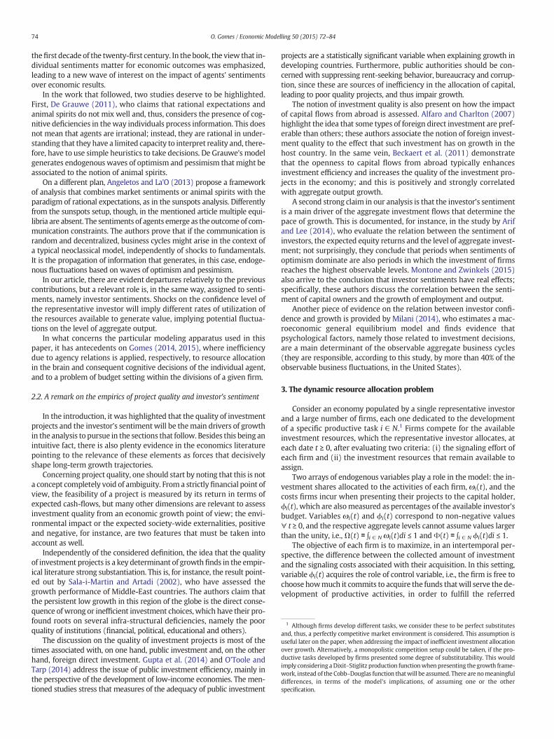
(iii) The steady-state value of the co-state variable, p∗, obeys constraint 2β−1β

1ρþζ ≤p

�b1

ρþζ if βN 12 or 0bp

�b 1ρþζ if β≤ 1

2.

Fig. 1. Steady-state uniqueness for the co-state variable.


The other differential equation of the system, Eq. (4), is obtained bysubstituting ϕi(t), as in Eq. (7), into the constraint Eq. (3):

ω�

i tð Þ ¼ B qi qβ= 1−βð Þi βBpi tð Þ½ �1= 1−βð Þ 1−Ω tð Þ½ �

n oh iβ1−Ω tð Þ½ �1−β−ζωi tð Þ⇔

ω�

i tð Þ ¼ B βBqipi tð Þ½ �β= 1−βð Þ 1−Ω tð Þ½ �−ζωi tð Þ⇔ω�

i tð Þ ¼ B1= 1−βð Þ βqipi tð Þ½ �β= 1−βð Þ 1−Ω tð Þ½ �−ζωi tð Þ:

The pair of differential Eqs. (4)–(5) is a deterministic two-dimensional dynamic system with two endogenous variables. A firststep in the process of evaluating this system's dynamics consists inassessing the properties of the steady-state.

Definition 3. Steady-state

The steady-state of theDRAP is the pointðω�i ; p

�i Þ ¼ fðω�

i ; p�i Þ : ω

�

iðtÞ ¼0; p

�

iðtÞ ¼ 0; i ∈Ng.Given the definition of the steady-state for the problem under

consideration, the following result is accomplished,

Proposition 2. The steady-state point of the DRAP, (ωi∗, pi∗), i ∈ N, exists

and it is unique.

Proof. Applying condition ṗi(t) = 0 to equation of motion Eq. (5),

1−βð Þββ= 1−βð ÞB1= 1−βð ÞZ

j ∈Nqβ= 1−βð Þj p�j

� �1= 1−βð Þ� �dj ¼ 1− ρþ ζð Þp�i :

ð10Þ

Observe that the lhs of expression Eq. (10) is the same independent-ly of the firm forwhich the optimality problem is approached. An imme-diate corollary of this observation is that pi∗= pj

∗,∀ i, j ∈N. In the light ofthis result, define p∗≡pi∗, ∀ i ∈ N, and rewrite Eq. (10) as

1−βð Þββ= 1−βð Þ Bp�ð Þ1= 1−βð ÞZ

j ∈Nqβ= 1−βð Þj dj ¼ 1− ρþ ζð Þp�: ð11Þ

Expression Eq. (11) does not allow for the determination of anexplicit solution for the steady-state level of the co-state variable. How-ever, it is straightforward to verify that this steady-state value exists andis unique. Begin by observing that the rhs of Eq. (11) is a straight linestarting at 1 (for p∗ = 0) and possessing a negative slope; while thelhs is an increasing convex function of p∗ starting at 0 (for p∗ = 0).Given the shape of the two mentioned functions, they will intersect ina single point for p ∈ð0; 1

ρþζÞ.To complete the proof, one needs to demonstrate that ωi

∗ exists andis unique as well. Solvingω

�

iðtÞ ¼ 0, given Eq. (4), the following relationemerges,

1−Ω� ¼ ζω�i

B1= 1−βð Þ βqip�i� β= 1−βð Þ ð12Þ

with Ω∗≡∫j ∈ N ωj∗dj. Because the steady-state value of the co-state

variable is identical across firms, Eq. (12) implies that, for any i, j ∈ N,

ω�i

ω�j¼ qi

q j

!β= 1−βð Þ: ð13Þ

Relation Eq. (13) allows for rewritingΩ∗, given the respective defini-tion,

Ω� ¼ 1qiβ= 1−βð Þ

Zj ∈N

qβ= 1−βð Þj djω�

i : ð14Þ

ReplacingΩ∗, as displayed in Eq. (14), into Eq. (12), the steady-stateof variable ωi(t) is given as

ω�i ¼

B1= 1−βð Þ βqip�ð Þβ= 1−βð Þ

B1= 1−βð Þ βp�ð Þβ= 1−βð ÞZ

j ∈Nqβ= 1−βð Þj djþ ζ

; i ∈N: ð15Þ

Since there is a unique p∗, expression Eq. (15) guarantees that aunique ωi

∗ exists as well. Nevertheless, note that ωi∗ is different across

firms, given the different quality of the projects presented to theinvestor.

Several elements in the proof of Proposition 2 deserve a comment.First, one can visualize the steady-state outcome for the co-statevariable through the graphical representation of the lhs and of the rhsof Eq. (10). The intersection point delivers p∗ as depicted in Fig. 1.

Second, note that the mechanics of the model impose an indisput-able upper bound on the value of p∗; one has stated, in Footnote 4,that this upper bound is required to guarantee that boundaries on thevalues of variables are respected. In fact, such upper bound does notneed to be forced into the model, since it arises spontaneously. Onewill get back to this issue later when directly exploring the feasibilityconditions of the model. A third point relates to Eq. (13). One shouldhighlight that it delivers a relevant result: it states that in the longterm steady-state the single determinant of the difference betweeninvestment shares allocated across firms is the quality of projectsignaling.

A last remark is associated with steady-state result (Eq. (15)). Onecan use this to obtain the expression of the aggregate investmentshare, also evaluated in the steady-state. Summing across all ωi

∗,

Ω� ¼B1= 1−βð Þ βp�ð Þβ= 1−βð Þ

Zi ∈N

qβ= 1−βð Þi di

B1= 1−βð Þ βp�ð Þβ= 1−βð ÞZi ∈ N

qβ= 1−βð Þi diþ ζ

: ð16Þ

Share Ω∗ can be represented, in an alternative form, once onecombines Eqs. (16) and (11),

Ω� ¼ 1− ρþ ζð Þp�1− ρþ βζð Þp� : ð17Þ

It is evident, both from Eqs. (16) and (17), that Ω∗ b 1. This result isimportant because it indicates that no matter the efficiency of theinvestment allocation process, the agency relation that is establishedbetween the investor and the firms will prevent investment resourcesto be fully allocated. Naturally, allocation results improve with a betterquality of the investment project proposals or with a more optimisticinvestor sentiment, as one will confirm with the formal analysis inSection 6; however, independently of the values of B and qi, there will


always be some waste of investment resources if they are allocatedunder the mechanics of the proposed dynamic model.

Another steady-state result is the one respecting the controlvariable. The evaluation of Eq. (7) in the steady-state, given the relationbetween p∗ and Ω∗ in expression Eq. (16), yields

ϕ�i ¼

1−βð Þζ βBð Þ1= 1−βð Þ p�ð Þ 2−βð Þ= 1−βð Þqβ= 1−βð Þi

1− ρþ βζð Þp� : ð18Þ

Note that, according to Eq. (18), the steady-state of the signaling costvariable differs across firms, given the difference in the quality of theproposed investment projects. For any i, j ∈ N,

ϕ�i

ϕ�j¼ qi

q j

!β= 1−βð Þ: ð19Þ

As for the budget share variable, the steady-state signaling costincurred by firm i relatively to the signaling cost incurred by firm j isas much larger as the wider is the difference in terms of the quality ofthe investment projects.

The steady-state value of the aggregate level of the signaling costsacross firms is obtainable directly from Eq. (18),

Φ� ¼Z

i ∈ Nϕ�i di ¼ βζp�Ω�: ð20Þ

5. Local stability

In this section, transitional dynamics of the DRAP are evaluated. Apoint (ωi0, pi0) in the vicinity of (ωi

∗, pi∗) is considered and local stabilityis approached through the linearization of the system of Eqs. (4)–(5).The linearization process requires the computation of the correspond-ing Jacobian matrix, which can be partitioned in four distinct blocks,

J ¼ J11 J12J21 J22

� �:

Matrix Jmn, m = 1, 2, n = 1, 2, will contain, as elements, the deriva-tives of each differential equation with respect to each variable, dulyevaluated in the steady-state. In matrix Jmn, one finds the derivativesof the state equations (m = 1) or of the co-state equations (m = 2)with respect to each state variable (n=1) or co-state variable (n=2).

The computation of the elements of the Jacobianmatrixwill allow forthe characterization of the stability properties of the dynamic system.

Proposition 3. The DRAP, when evaluated in the steady-state vicinity,delivers a saddle-path stable equilibrium, with the number of stabletrajectories equal to the number of productive tasks (i.e., the numberof firms).

Proof. Local stability is approachable by computing the eigenvalues ofthe Jacobian matrix. Stable and unstable dimensions have correspon-dence on the signs of the eigenvalues. Specifically, to each negative(positive) eigenvalue, it corresponds a stable (unstable) dimension ofthe model.

Note that the Jacobian matrix is a square matrix of order equal totwice the number of firms or productive tasks. The Jacobian matrixwill contain a number of eigenvalues equal to thematrix order. These ei-genvalues are straightforward to compute because J21 is a matrix ofzeros.5 In this case, the eigenvalues of J are necessarily the eigenvaluesof matrices J11 and J22; hence, the contents of J12 are not relevant forthe purpose at hand, and one does not need to calculate them.

5 Equations relating the co-state variables dependon this variables alone, andnot on thestate variables.

Matrix J11 has, as elements in the main diagonal, the following,

~jii ¼ −1−Z

j ∈ N if gω�

jd j

1−Z

j ∈ Nω�

j djζ :

Outside the main diagonal, the elements are

~ji‘ ¼ −ω�

i

1−Z

j ∈ Nω�

j djζ :

Relatively to matrix J22, the respective elements are, in the maindiagonal,

~jii ¼ ρþ1−Z

j∈Nn if gω�

j d j

1−Z

j ∈ Nω�

j djζ :

Outside the main diagonal of J22,

~ji‘ ¼ −ω‘

�

1−Z

j ∈ Nω�

j djζ :

For matrix J11, one of the eigenvalues is

λi ¼ −1

1−Z

j ∈Nω�

j d jζ :

All the others are identical,

λ j ¼ −ζ ; j∈N if g:

A similar result is obtained for J22,

λi ¼ ρþ 1

1−Z

j ∈ Nω�

j djζ

and

λ j ¼ ρþ ζ ; j∈N if g:

Direct observation indicates that the eigenvalues of J11 are all nega-tive and that the eigenvalues of J22 are all positive. Therefore, the systemis saddle-path stablewith stable and unstable spaces possessing an iden-tical dimension. The dimensionality of both the stable and the unstabletrajectories is equal to the number of firms that compete for the invest-ment resources. Therefore, there exists a saddle-point equilibrium,with this point having a dimensionality equal to the number of firms.

To address transitional dynamics, one needs to compute the analyt-ical expressions of the stable trajectories through which the endoge-nous variables converge to the long-term equilibrium point. A firstrelevant result involves the (absence of)motion of the co-state variable.

Proposition 4. In the convergence towards the steady-state, the co-state variable assumes the constant value pi(t) = p∗.

Proof. For a given firm i, the stable trajectory respecting to the co-statevariable pi(t) is given by the following general expression,

pi tð Þ−p� ¼Z

j ∈N

Z‘∈N

χp‘iχ

ω;−1j‘ d‘

�ω j tð Þ−ω�

j

h i� �dj; i ∈N ð21Þ


where χ‘ip and χj‘

ω,− 1 are elements of the matrices Ξp and Ξω−1. Matrix

Ξp is the sub-matrix of the matrix of eigenvectors of the Jacobian Jthat is associated to the negative eigenvalues and that respects to theco-state variables;Ξω

−1 is the inverse of the sub-matrix of the samema-trix of eigenvectors that respects to the state variables. Thematrix of ei-genvectors concerning negative eigenvalues is Ξ ¼ ½Ξω Ξp �0.

Taking into consideration the eigenvalues of J, the followingoutcome is obtained: Ξp ¼ 0, i.e., all elements χ‘i

p are null values. Thisimplies that expression (21) reduces to pi(t) = p∗, ∀ i ∈ N, meaningthat in the convergence to the steady-state following the stable trajecto-ry, the co-state variable is initially placed at point pi0 = p∗ and remainsthere as variable ωi(t) converges towards its long-term value.

The result in Proposition 4 simplifies significantly the analysis of theDRAP, since one can focus solely on the movement of ωi(t). In theadjustment to the steady-state, Eq. (4) becomes a linear equation,

ω�

i tð Þ ¼ B1= 1−βð Þ βqip�ð Þβ= 1−βð Þ 1−Ω tð Þ½ �−ζωi tð Þ; i ∈N ð22Þ

that, under steady-state conditions, is equivalent to

ω�

i tð Þ ¼ ζω�i

1−Ω� 1−Ω tð Þ½ �−ζωi tð Þ; i ∈N: ð23Þ

The solution of Eq. (23) for the set of all productive tasks i is,

ω ¼ ω� þΞωexp Λtð ÞΞ−1ω ω0−ω�ð Þ: ð24Þ

In expression (24), ω is the vector of state variables ωi(t), i ∈ N; ω0

and ω∗ are the respective vectors of initial values and steady-statevalues. Matrix Ξω is the matrix of eigenvectors of J11 and Ξω

−1 itsinverse, as defined above; Λ is the Jordan matrix of the system, i.e., itis a matrix with the system's eigenvalues in the main diagonal andzeros outside the main diagonal.

Proceeding with the respective computation, the system's solutionfor each share ωi(t) is derived,

ωi tð Þ ¼ ω�i þ

ω�i

Ω� exp −ζ

1−Ω� t �

−exp −ζtð Þ� �

þ ωi0−ω�i

� exp −ζtð Þ; i ∈N: ð25Þ

The sum of ωi(t) across the investment shares of all firms deliversthe trajectory in time of the aggregate investment share Ω(t),6

Ω tð Þ ¼ Ω� þ Ω0−Ω�ð Þexp −ζ

1−Ω� t �

: ð26Þ

Next, one proves that the first-order conditions in the proof ofProposition 1 effectively are the relevant optimality conditions of theproblem, under the assumptions that were mentioned in the proof ofProposition 1.

Proposition 5. Let Ω0 b Ω∗, p(t) = p∗ and

p� :

2β−1β

1ρþ ζ

≤p�b1

ρþ ζif βN

12

0bp�b1

ρþ ζif β≤

12:

8>><>>:Under these conditions, constraints on variables ωi(t) ≥ 0, ϕi(t) ≥ 0,

and Ω(t) ≤ 1, Φ(t) ≤ 1 are satisfied, ∀ t ≥ 0.

Proof. The initial value and the steady-state value ofΩ(t) are such that0 b Ω0 b Ω∗ b 1. Eq. (26) implies Ω(t) = Ω0 for t = 0, Ω(t) = Ω∗ when

6 The trajectory of the aggregate investment share (Eq. (26)) could be obtained, as well,through the determination of the solution of the scalar differential equation respectingΩ(t), which is Ω

� ðtÞ ¼ − ζ1−Ω� ½ΩðtÞ−Ω��. This differential equation is obtained directly

from the definition Ω� ðtÞ≡∫i∈N ω

�

iðtÞdi, with ω�

iðtÞ given by Eq. (23).

t→+ ∞, and Ω0 b Ω(t) b Ω∗, for 0 b t b+ ∞. Therefore, it is not possibleto have any value of the aggregate investment share above 1; further-more, Eq. (25) indicates that ωi(t) must be a non-negative value,independently of the assumed time moment; to confirm this outcome,note that Ω0 b Ω∗ by assumption and that expð− ζ

1−Ω� tÞbexpð−ζtÞ forany t, thus making the second term of the expression positive; becausethe sum of the remaining terms, ωi

∗ + (ωi0 − ωi∗)exp(−ζt) must be

positive as well, regardless of t, one also confirms the veracity ofωi(t) ≥ 0.

Under pi(t) = p∗, expression Eq. (7) is equivalent to

ϕi tð Þ ¼ qβ= 1−βð Þi βBp�ð Þ1= 1−βð Þ 1−Ω tð Þ½ �; i ∈N: ð27Þ

The control variable is, according to Eq. (27), a non-negative value.Finally, the sum of ϕi(t) as presented in Eq. (27), and given the steady-state relations, takes the form

Φ tð Þ ¼ β1−β

1− ρþ ζð Þp�½ � 1−Ω tð Þ½ �: ð28Þ

In Eq. (28), Ω(t) may assume any value between 0 and 1. Therefore,conditionΦ(t) ≤ 1 is guaranteedwhenever β

1−β ½1−ðρþ ζÞp��≤1. Solvingthe inequality with respect to p∗, it yields p�≥ 2β−1

β1

ρþζ . If β ≤ 1/2, theconstraint is necessarily satisfied, because of the non-negativity of p∗;the condition must be imposed in the opposite case, i.e., β N 1/2.

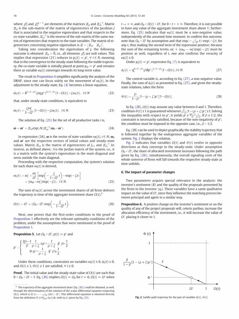
Eq. (28) can be used to depict graphically the stability trajectory thatis followed together by the endogenous aggregate variables of thesystem. Fig. 2 displays the relation,

Fig. 2 indicates that variables Ω(t) and Φ(t) evolve in oppositedirections as they converge to the steady-state. Under assumptionΩ0 b Ω∗, the share of allocated investment increases following the pathgiven by Eq. (26); simultaneously, the overall signaling costs of thewhole universe of firms will fall towards the respective steady-state astime unfolds.

6. The impact of parameter changes

Two parameters acquire special relevance in the analysis: theinvestor's sentiment (B) and the quality of the proposals presented bythe firms to the investor (qi). These variables have a same qualitativeimpact on the value ofΩ∗, since they influence thematching process be-tween principal and agent in a similar way.

Proposition 6. A positive change on the investor's sentiment or on thequality of any of the project proposals will, ceteris paribus, increase theallocation efficiency of the investment, i.e., it will increase the value ofΩ∗, placing it closer to 1.

Fig. 2. Saddle-path trajectory for the pair of variables Ω(t), Φ(t).

Fig. 4. Effect of a change on ρ or ζ over p⁎.


Proof. Recover the steady-state value of Ω(t) in expression Eq. (17).The differentiation of this expression with respect to B or qi yields

∂Ω�

∂B¼ −

1−βð Þζ1− ρþ βζð Þp�½ �2

∂p�

∂Bð29Þ

or

∂Ω�

∂qi¼ −


∂p�

∂qi: ð30Þ

Since a general explicit expression for p∗ was not determined, onecannot derive ∂p�

∂B and ∂p�

∂qiexplicitly. However, a qualitative evaluation

of the signs of these derivatives is possible. Returning to equilibriumequality Eq. (11), one observes that a change on B or qi will not exertinfluence over the rhs expression of the equation. Relatively to the lhs,a positive variation on the value of any of the two parameters willturn the slope of the respective function more pronounced, makingthe lhs and the rhs to intersect at a lower value of p∗, as depicted in Fig. 3.

The figure reveals that ∂p�

∂B b0 and ∂p�

∂qib0 and, therefore, one concludes

that a positive sentiment change on the quality of any of the projectspresented to the investor will improve the efficiency of the resourceallocation: ∂Ω�

∂B N0; ∂Ω�

∂qiN0:

Other two parameters have a substantive influence over the value ofΩ∗. These are the intertemporal discount rate (ρ) and the percentage ofthe allocated budget that the investor recovers in each period (ζ). Forthese parameters, the following results apply,

Proposition 7. A positive change on the values of parameters ρ and ζhave a qualitatively ambiguous effect over Ω∗.

Proof. Start by noticing that a positive change on ρ or ζ will imply areduction on the steady-state value of the co-state variable. This occursbecause in the relation between the lhs and the rhs of Eq. (11), the firstdoes not suffer any change as a result of varying ρ or ζ, while the rhswillrotate inward for higher values of each of the two parameters. Fig. 4clarifies this point.

To evaluate the effect that the change in any of the parameters underconsideration exerts on Ω∗, one computes the derivatives of Eq. (17)with respect to each of the two parameters,

∂Ω�

∂ρ¼ −


∂p�

∂ρþ p�ð Þ2

�ð31Þ

∂Ω�

∂ζ¼ −


∂p�

∂ζþ 1−ρp�

ζp�

�: ð32Þ

Fig. 3. Effect of a change on B or qi over p⁎.

Since the signs of terms ∂p�

∂ρ þ ðp�Þ2 and ∂p�

∂ζ þ 1−ρp�ζ p� are not deter-

minable for the general version of the model, one cannot conclude onthe qualitative impact of changes on ρ and ζ over Ω∗.

To illustrate the potential of the DRAP in explaining investment allo-cation, consider a numerical example. Let β=0.25, ∫i ∈ Nqi

β/(1 − β)di=1,B= 2, ρ= 0.04, ζ = 0.05.7 For these values, Eq. (11) indicates that thesteady-state level of the co-state variable is, approximately, p∗=0.8279.Taking Eqs. (17) and (20), one also determines the steady-state of theaggregate state and control variables: Ω∗ = 0.9675 and Φ∗ = 0.01. Inthis case, for the assumed parameter values, 96.75 % of the availableinvestment resources are effectively allocated, in the long-run, to theproductive activities and, on the aggregate, firms will need to spend1 % of the available resources to attain this outcome.

The stable path between Ω(t) and Φ(t) is, following (28), Φ(t) =0.3085[1− Ω(t)]. The stable trajectory, for the specific example underappreciation, is displayed in Fig. 5.

Under the assumptionΩ0 bΩ∗, only the segment 0 ≤Ω(t) ≤ 0.9675, inFig. 5, matters. In this segment, a one unit positive change on the aggre-gate investment share implies a decrease in the value of the aggregatecontrol variable on an amount 0.3085, as the convergence to thesteady-state takes place.

The example might be employed as well to quantitatively assess theimpact of changes on parameter values and to confirm the generalresults presented earlier in this section. Consider first a positive changeon the sentiment value, ΔB= 0.05. Recomputing the steady-state levelof the co-state variable, one obtains p(Bnew)

∗ =0.8088. Hence, the changeon p∗ with origin in the positive sentiment evolution is Δp∗ =−0.0191.Resorting to expression Eq. (17), one verifies thatΩ(Bnew)

∗ =0.9683 and,thus, ΔΩ∗ = 0.0008, i.e., the allocation of resources as improved in 0.8percentage points.

Consider, in a second moment, a change on the intertemporaldiscount rate. Let Δρ = −0.02. In this case, firms become more patientin the way they evaluate future outcomes. Now, p(ρnew)

∗ = 0.8385. Asdiscussed earlier, a decrease in ρmust translate on a higher value of theco-state variable steady-state level; in this case, Δp∗ = 0.0106.Replacing, in Eq. (17), the new values of ρ and p∗, one obtains thedisturbed steady-state level of the aggregate investment share,Ω(ρnew)∗ =0.9677. For the assumedparameterization, the negative change

on the discount rate has provoked a slight positive variation onΩ∗,ΔΩ∗=0.0002;more patience is, in this case, synonymous of an environment ca-pable of generating a more efficient long-term allocation of resources.

7 The values used in the example are adopted with the objective of fulfilling twocriteria: to be empirically plausible and to deliver sensible investment allocation andgrowth outcomes. Note, however, that some of the parameters are hard to measure andthat they can be presented in different scales, as it is the case of the sentiment index, thequality of projects or the matching elasticity.

Fig. 5. Illustration of the saddle-path trajectory.


7. Neoclassical growth under inefficient investment allocation

In this section, the DRAP, as previously examined, is applied tothe standard neoclassical growth model. One builds a Ramsey–Cass–Koopmans (RCK) optimal control problemwhere the possibility of inef-ficient investment allocation is considered.

Definition 4. RCK/DRAP growth model

Consider a representative agent for whom the objective function is

V 0ð Þ ¼ Maxc tð Þ

Z þ∞

0u c tð Þ½ �exp −ρtð Þdt: ð33Þ

In Eq. (33), c(t) ≥ 0 represents consumption and u(.) is the utilityfunction. The same intertemporal discount rate ρ as for the DRAPproblem is assumed. Optimal control problem (Eq. (33)) is subject tothe capital accumulation constraint

k�

tð Þ ¼ f k tð Þð Þ−c tð Þ½ �Ω tð Þ−δk tð Þ; k 0ð Þ ¼ k0 given: ð34Þ

Variable k(t) ≥ 0 represents physical capital per unit of labor,δ ∈ (0, 1) is the depreciation rate of capital and f(k(t)) is the productionfunction. V(0), in Eq. (33), subject to Eq. (34), is the RCK/DRAP growthmodel.

Observe that the single difference between the RCK/DRAP modeland the original formulation of the RCK growth model is the presenceofΩ(t) in the expression of the resource constraint. Instead of consider-ing a measure of potential gross investment, which corresponds to thedifference between output, given by the production function, andconsumption, effective gross investment is assumed; this relates to thepotential level times the aggregate investment share Ω(t), a variablefor which the respective dynamics were approached in previoussections. The remaining share, [f(k(t)) − c(t)][1 − Ω(t)] should beinterpreted as inefficient investment, i.e., investment with zero return,since, as discussed, it has no productive end.

As it is common in growth models, and in order to facilitate theanalytical exploration of the underlying dynamics, let us consider atypical constant intertemporal elasticity of substitution utility function,

U½cðtÞ� ¼ cðtÞ1−θ−11−θ ; θ ∈ (0, + ∞)\{1}, with 1/θ the intertemporal elasticity

of substitution for consumption; assume, as well, a standard Cobb–Douglas production function, f(k(t)) = Ak(t)α, with A N 0 the state oftechnology and α ∈ (0, 1) the output–capital elasticity.

In what follows, the neoclassical growth model is solved for theeffective gross investment version and the main results are discussed.

Proposition 8. The optimal trajectory of consumption is, on theRCK/DRAP growth model, given by equation

c�tð Þ ¼ 1

θ

�αAk tð Þ− 1−αð ÞΩ tð Þ−B1= 1−βð Þββ= 1−βð Þ

Zi∈N

qipi tð Þ½ �β= 1−βð Þdi

×1−Ω tð ÞΩ tð Þ − ρþ δð Þ þ ζgc tð Þ:

ð35Þ

Proof. The current-value Hamiltonian function of this problem is,

H k tð Þ; c tð Þ; ~p tð Þ½ � ¼ c tð Þ1−θ−11−θ

þ ~p tð Þ Ak tð Þα−c tð Þ� Ω tð Þ−δk tð Þ� � ð36Þ

with ~pðtÞ the co-state variable associated with k(t). First-orderconditions are

∂H∂c tð Þ ¼ 0⇒ c tð Þ−θ ¼ ~p tð ÞΩ tð Þ ð37Þ

~p�

tð Þ ¼ ρ~p tð Þ− ∂H∂k tð Þ⇒

~p�

tð Þ ¼ ρþ δð Þ~p tð Þ−αA~p tð Þk tð Þ− 1−αð ÞΩ tð Þð38Þ

and the transversality condition,

limt→þ∞

~p tð Þexp −ρtð Þk tð Þ ¼ 0: ð39Þ

The differentiation of Eq. (37) with respect to time yields

−θc�tð Þ

c tð Þ ¼ ~p�

tð Þ~p tð Þ þ

Ω�

tð ÞΩ tð Þ ð40Þ

Growth rate ~p�

ðtÞ~pðtÞ is obtainable from Eq. (38), while Ω

� ðtÞΩðtÞ corresponds to

the aggregate version of Eq. (4). Replacing these two growth rates inEq. (40), the rule of motion for consumption, Eq. (35), is obtained.

Because the DRAP was solved independently of the growth model,one may assume that the respective stable trajectory is followed,i.e., according to Proposition 4, pi(t)= p∗. In this case, Eq. (35) simplifiesto

c�tð Þ ¼ 1

θαAk tð Þ− 1−αð ÞΩ tð Þ−ζ

Ω�

1−Ω� :1−Ω tð ÞΩ tð Þ − ρþ δð Þ þ ζ

� �c tð Þ: ð41Þ

The dynamic analysis of the RCK/DRAPmodel is feasible through theevaluation of a three-dimensional system involving the constraint oncapital accumulation, Eq. (34), the consumption differential equation,Eq. (14), and the differential equation for Ω(t), that one can recoverfrom Footnote 3.

To proceed, one defines the steady-state of the RCK/DRAP.

Definition 5. Steady-state of the RCK/DRAP growth model

The steady-state of the RCK/DRAP is the point

k�; c�;Ω�ð Þ ¼ k�; c�;Ω�ð Þ :k�

tð Þ ¼ 0; c�tð Þ ¼ 0;Ω

�

tð Þ ¼ 0n o

:

Adopting the above definition, the result in Proposition 9 isaccomplished.

Proposition 9. The steady-state of the neoclassical growth model withagency relations in the allocation of investment exists and it is unique.The steady-state values of the capital and of the consumption variablesare, respectively,

k� ¼ k�P Ω�ð Þ1= 1−αð Þ; c� ¼ c�P Ω�ð Þα= 1−αð Þ


with kP∗ and cP

∗ representing the long-term potential levels of capital andconsumption, i.e., the steady-state levels of the two variables whenthere is full efficiency in the allocation of investment. The respectivevalues are,

k�P ¼ αAρþ δ

�1= 1−αð Þ; c�P ¼ 1

αρþ 1−α

αδ

�αAρþ δ

�1= 1−αð Þ:

Proof. Applying Definition 5 to differential Eqs. (34) and (41), it yields,respectively,

c� ¼ A k�ð Þα−δk�

Ω� ð42Þ

k� ¼ αAΩ�

ρþ δ

�1= 1−αð Þ: ð43Þ

Result Eq. (43) is the one presented in the proposition for the phys-ical capital variable. Value c∗ is accomplished by replacing k∗ in Eq. (43)into Eq. (42),

c� ¼ 1αρþ 1−α

αδ

�αAρþ δ

�1= 1−αð ÞΩ�ð Þα= 1−αð Þ

: ð44Þ

The graphical inspection of the steady-state result is undertaken viaFig. 6. In this graphic, it is represented a curve that indicates the positionof the growth model steady-state (k∗, c∗) for every possible value of Ω∗.One visually confirms that the typical result of the neoclassical growthmodel is a particular case of our more complete structure of analysis,namely the limiting case for which there is a perfect allocation of invest-ment resources.

The concave shape of the line in Fig. 6 points out that lessthan full efficiency on investment allocation penalizes relatively morethe capital stock than the level of consumption, in the steady-state.

To address transitional dynamics in the RCK/DRAP, take Eqs. (34),(41), and the equation for the dynamics of Ω(t). In the vicinity of thesteady-state, a linearized representation of the system under apprecia-tion will be

k�

tð Þc�tð Þ

Ω�

tð Þ

264

375 ¼

ρ −Ω� δk�

Ω�

−1−αθ

ρþ δð Þ c�

k�0

1θ

ρþ δþ ζ1−Ω�

�c�

Ω�

0 0 −ζ

1−Ω�

2666664

3777775

�k tð Þ−k�

c tð Þ−c�

Ω tð Þ−Ω�

24

35: ð45Þ

Fig. 6. Steady-state (k⁎, c⁎) for different values of Ω⁎.

Matricial system Eq. (45) allows for an assessment of the stabilityproperties of the growth model.

Proposition 10. The long-term equilibrium of the RCK/DRAP is saddle-path stable.

Proof. The Jacobian matrix of system Eq. (45) possesses three eigen-values. One of them relates to the investment share and it confirmsthe stable nature of the steady-state valueΩ∗ (this is the eigenvalueλ ¼− ζ

1−Ω� b0). To evaluate the stability of the growth model, one canconcentrate attention on the sub-matrix of the Jacobian relating tocapital and consumption variables. The eigenvalues of the respectivesub-matrix are such that

λk;c1 λk;c

2 ¼ −1−αθ

ρþ δð Þ c�

k�Ω� b 0

λk;c1 þ λk;c

2 ¼ ρ N 0:

The product of the eigenvalues, which corresponds to the determi-nant of the matrix, is negative, while the sum of the eigenvalues,which is the trace of the Jacobian, takes a positive value. In this case,therewill be, necessarily, a positive eigenvalue and a negative eigenval-ue, meaning that, as in the original Ramsey model, a saddle-path stableequilibrium prevails.

Let us consider the sub-system of Eq. (45) relating variables k(t) andc(t). Given the relations involving the eigenvalues in the proof ofProposition 10, the sub-system can be written under the form

k�

tð Þc�tð Þ

" #¼

λk;c1 þ λk;c

2 −Ω�

λk;c1 λk;c

2Ω� 0

264

375 k tð Þ−k�

c tð Þ−c�

� �: ð46Þ

Let λ1k,c be the negative eigenvalue and λ2

k,c the positive eigenvalue.

In this case,Ξk;c ¼ ½ Ω�

λk;c2

1 �0 is the eigenvector associated to the negative

eigenvalue. As a result, the expression of the one-dimensional stabletrajectory in the k(t), c(t) locus is

c tð Þ−c� ¼ λk;c2Ω� k tð Þ−k�½ �: ð47Þ

The saddle trajectory has a positive slope, meaning that in the ad-justment from (k0, c0) towards (k∗, c∗), both variables will exhibit asame qualitative behavior. Again, the full efficiency on the allocationof investment is a particular case of (47), for Ω∗ = 1. Therefore, oneconcludes that the more efficient the investment allocation is, the lesssteeper the saddle-path trajectory will be. Under strong inefficiency, asmall change on the stock of capital will provoke a significant changeon the level of consumption, as the adjustment towards the steady-state unfolds.

Growth dynamics can be graphically evaluated through the

construction of the respective phase diagram. The lines forwhichk�

ðtÞ ¼0 and ċ(t) = 0 are, respectively, cðtÞ−c� ¼ λk;c

1 þλk;c2

Ω� ½kðtÞ−k�� and k(t) =

k∗. Directional arrows in the four quadrants formed by the lines k�

ðtÞ ¼0 and ċ(t) = 0 are determined by the elements in the first column ofthe matrix in Eq. (46) and point in the same directions as those in theoriginal Ramsey model phase diagram.8 Fig. 7 represents the phasediagram forΩ∗ b 1, making the proper comparison with the benchmarkcase Ω∗ = 1.

In Fig. 7, one should highlight the difference of position between thesaddle-path for Ω∗ b 1 (S) and the saddle-path for Ω∗ =1 (SP). They areboth positively sloped trajectories, but the first is necessarily steeper

8 See Barro and Sala-i-Martin (2004), chapter 2.

Fig. 7. Phase diagram for the neoclassical growth model under inefficiency on the alloca-tion of investment.

Fig. 8. Effect of a positive investor's sentiment change on the steady-state levels of physicalcapital and consumption.


than the second. The position of the steady-state points, in each of thetwo cases, is represented over the steady-state curve drawn in Fig. 6.

One final appointment in this section goes to the impact of asentiment shock over the dynamics of capital accumulation and con-sumption. Intuitively, following the result in Proposition 6, accordingto which a positive change on the investor's sentiment or confidencewill increase the efficiency on the allocation of investment resourcesto production tasks, it is clear that an upward movement over the linerepresented in Fig. 6 will occur. This is depicted in Fig. 8.

A discrete shock on the investor's sentiment, as one visualizes inFig. 8, implies an instantaneous jump from the original steady-state tothe saddle-path that is formedwith the sentiment disturbance. The im-mediate adjustment takes place on the value of the control variable,i.e., consumption, and once the new saddle-path is accomplished, bothvariables, capital and consumption, will follow this stable trajectoryuntil the new steady-state point is reached. Note that in this casethere is an instantaneous fall in consumption that comes in thesequence of the positive sentiment shock, given the position of the sta-ble trajectory. The consumption level will then increase with capital tothe new steady-state, where both variables will possess higher valuesthan in the pre-shock situation. The short-run fall in consumptionmight be explained under the idea that a better investor's sentimentimplies a reorganization of the productive activity that has its first pos-itive impact over the accumulation of capital, while an increase in theproduction of consumption goods will occur only in a long-termperspective.

The impact of the sentiment change can be quantified through thecomputation of short-run and long-run multipliers. Rewrite systemEq. (46) with a vector of exogenous coefficients concerning parameterB,

k�

tð Þc�tð Þ

" #¼

λk;c1 þ λk;c

2 −Ω�

λk;c1 λk;c

2

Ω� 0

264

375 k tð Þ−k�

c tð Þ−c�

� �þ

δk�

Ω�∂Ω�

∂Bρþ δθ

c�∂Ω�

∂B

2664

3775ΔB: ð48Þ

Let Jk,c be the Jacobian matrix in system Eq. (46). Long-run multi-pliers are,

Δk ∞ð ÞΔc ∞ð Þ� �

¼ − Jk;c� −1

δk�

Ω�∂Ω�

∂Bρþ δθ

c�∂Ω�

∂B

2664

3775ΔB ¼

k�

1−α∂Ω�

∂B

δþ 11−α

�k�

∂Ω�

∂B

2664

3775ΔB

ð49Þ

Since ∂Ω�∂B N0 (see Proposition 6), one confirms the graphical result

such that a positive sentiment change generates an increase, in a long-term perspective, both on the stock of accumulated capital and on thesteady-state level of consumption.

One can also measure the short-run effect over the consumptionvariable, since this suffers, in line with what Fig. 8 shows, an initialjump from the first to the second stable trajectory. Assuming that theshock on B is permanent and non-anticipated, the respective multiplieris

Δc 0ð Þ ¼ Δc ∞ð Þ−λk;c2Ω� Δk ∞ð Þ

" #ΔB

¼ δþ 11−α

1−λk;c2Ω�

!" #k�

1−α∂Ω�

∂BΔB:

ð50Þ

The sign of Eq. (50) is ambiguous. Because the slope of the newsaddle-path, after the positive disturbance on the value of B, diminishes,consumption may increase or fall immediately after the shock. In Fig. 8,the consumption level suffers an instantaneous decrease; however,

different parameter values could generate the opposite result, leadingto an outcome as the one illustrated in Fig. 9.

8. Endogenous growth under inefficient investment allocation

Consider now an endogenous growth environment,

Definition 6. AK/DRAP growth model

The problem in Definition 4 acquires the quality of endogenousgrowth model for an output–capital elasticity equal to 1.

Assuming α = 1, the capital accumulation equation is

k�

tð Þ ¼ AΩ tð Þ−δ½ �k tð Þ−c tð ÞΩ tð Þ; k0 given ð51Þ

and, taking p(t) = p∗, the differential equation for the motion of theconsumption becomes

c�tð Þ ¼ 1

θAΩ tð Þ−ζ

Ω�

1−Ω� :1−Ω tð ÞΩ tð Þ − ρþ δð Þ þ ζ

� �c tð Þ: ð52Þ


Under endogenous growth, the steady-state acquires new features.

Definition 7. Steady-state in the AK/DRAP model

In the AK/DRAP model, capital and consumption grow at a samepositive rate in the steady-state,γ :¼ k

�

k ¼ c�

c. The ratio between consump-tion and capital must, thus, be constant in the steady-state: forψðtÞ≡ cðtÞ

kðtÞ,the steady-state is such that ψ� ¼ fψ� :ψ

� ðtÞ ¼ 0g.Applying Definition 7,

Proposition 11. In the steady-state of the AK/DRAP model, the ratioconsumption-capital is the constant value

ψ� ¼ θ−1ð Þ AΩ�−δð Þ þ ρθΩ� ð53Þ

and capital and consumption grow at rate γ ¼ 1θ ½AΩ�−ðρþ δÞ� .

Condition Ω�N ρþδA is required to guarantee positive long-term endoge-

nous growth.

Proof. Growth rate γ, as displayed in the proposition, can be obtaineddirectly from Eq. (52). In fact, c

�

c ¼ 1θ ½AΩ�−ðρþ δÞ�. The expression of

the differential equation for ratio ψ(t) is obtained by noticing that ψ� ðtÞψðtÞ ¼

c� ðtÞcðtÞ−

k�

ðtÞkðtÞ. Such expression is

ψ�

tð Þ ¼ 1−θθ

AΩ tð Þ−1θζ

Ω�

1−Ω� :1−Ω tð ÞΩ tð Þ −

1θ

ρ−ζð Þ þ θ−1θ

δþ ψ tð ÞΩ tð Þ� �

ψ tð Þ:

ð54Þ

The evaluation of Eq. (54) in the steady-state delivers the value ofthe long-term consumption-capital ratio in the modified AK model.The result is value Eq. (53) in the proposition. Note that ψ∗ is necessarilya positive value given the constraint that also guarantees a positivelong-term growth rate.

Expression Eq. (53) indicates that in the AK/DRAP model, the con-sumption–capital ratio in the steady-state depends on the value of Ω∗.

Observe that ∂ψ�

∂Ω� ¼ ðθ−1Þδ−ρθðΩ�Þ2 . We identify two cases,

• if (θ − 1)δ N ρ, then ψ∗ increases with a positive change in Ω∗;• if (θ − 1)δ b ρ, then ψ∗ decreases with a positive change in Ω∗.

The results point to the intuition that a relatively patient agent (lowρ)will, in the steady-state, see the consumption level increase relativelyto the capital stock when the efficiency on the allocation of the

Fig. 9. Effect of a positive investor's sentiment change on the steady-state, without con-sumption undershooting.

investment increases, and vice-versa. Fig. 10 illustrates the steady-state relation between variables Ω(t) and ψ(t).

Relatively to transitional dynamics, note that in the steady-statevicinity, the AK/DRAP model has correspondence in the following sys-tem,

ψ�

tð ÞΩ�

tð Þ

" #¼

Ω�ψ� ψ�ð Þ2− θ−1θ

Aψ� þ ζθ

11−Ω�ð ÞΩ�

0 −ζ

1−Ω�

2664

3775 ψ tð Þ−ψ�

Ω tð Þ−Ω�

� �: ð55Þ

Eigenvalues are λ1ψ,Ω =Ω∗ψ∗ N 0 and λψ;Ω2 ¼ − ζ

1−Ω� b0, and, thus, thesteady-state is saddle-path stable. Observe that the motion of Ω(t) isindependent of ψ(t), what implies that, in the convergence towardsthe steady-state, the consumption-capital ratio is chosen such that it re-mains undisturbed in the steady-state value (ψ(t) = ψ∗), i.e., only thedynamics of Ω(t), as mentioned in Section 5, matters.

A last remark goes to the effect of a sentiment change over thesteady-state of the AK/DRAP model. Because ΔB N 0 implies ΔΩ∗ N 0, apositive change on the investor's sentiment triggers a larger steady-state growth rate for the main economic indicators, i.e., capital andconsumption. The effect of a change on sentiment over the steady-state growth rate is as much larger as the better is the state of technol-ogy and the higher is the intertemporal elasticity of substitution for con-

sumption. Given that ∂ψ�

∂Ω� does not have an unequivocal sign one cannotassert, unambiguously, which is the impact of a sentiment change overthe consumption–capital steady-state ratio.

9. Conclusion

Neoclassical and endogenous growth models offer a compellingexplanation on how the economy accumulates physical capital and onwhich is the consumption trajectory in time that maximizes utility.These models have, as an underlying assumption, the notion that in-vestment is always allocated efficiently and all investment resourcesare used in production in every time moment. In such a setting, theeconomy is in a position of full employment of resources.

In this paper, one askswhat are the growth implications of assumingan investment allocation process subject to inefficiencies that originateon an agency relation between a representative investor and a largenumber of firms that compete for financial resources to develop theiractivities. The investment problem explains how some investment re-sources are left unused at each time period provoking an inefficiencythatwill certainly influence the growth process. Assuming inefficient in-vestment allocation, long-term capital and consumption levels will fallbelow the full efficiency levels, in the neoclassical model, and thelong-term growth rate will also be lower than in the benchmark case,when taking the AK endogenous growth model.

The investment allocation problem is designed such that theinvestor's sentiment plays a relevant role. Sentiments enter the modelvia the matching between resource demand from firms and resourcesupply by the investor. An upgrade in the investor's sentiment will in-crease the efficiency allocation, producing as well a result in terms ofgrowth outcomes closer to what the original Ramsey–Cass–KoopmansandAKmodels show. This setting is appropriate to study business cyclesin the environment typically considered by growth theorists: changeson sentiments provoke changes on growth outcomes.

Future research on the theme of this papermay follow various direc-tions. Three suggestive paths for further inquiry include an explicit con-sideration of the dynamics of project quality evolution; the design of anetwork of social contact among firms that may influence the degreeof optimism or pessimism of the representative investor; and the adap-tation to an open economy scenario where the representative investormay choose to invest domestically or abroad, providing different financ-ing conditions for firms in each location.

A) B)

Fig. 10. Steady-state relation between Ω⁎ and ψ⁎.


References

Agliardi, E., Agliardi, R., 2008. Progressive taxation and corporate liquidation policy. Econ.Model. 25, 532–541.

Akerlof, G.A., Shiller, R.J., 2009. Animal Spirits: How Human Psychology Drives the Econ-omy, andWhy It Matters for Global Capitalism. Princeton University Press, Princeton,NJ.

Albuquerque, R.,Wang, N., 2008. Agency conflicts, investment, and asset pricing. J. Financ.63, 1–40.

Alfaro, L., Charlton, A., 2007. Growth and the quality of foreign direct investment: is all FDIequal? CEP Discussion Paper No. 0830

Angeletos, G.M., La'O, J., 2013. Sentiments. Econometrica 81, 739–779.Arif, S., Lee, C.M.C., 2014. Aggregate investment and investor sentiment. Graduate School

of Business Research Paper No. 3061. Stanford University.Azariadis, C., 1981. Self-fulfilling prophecies. J. Econ. Theory 25, 380–396.Barro, R.J., Sala-i-Martin, X., 2004. Economic Growth. 2nd edition. MIT Press, Cambridge,

MA.Beckaert, G., Harvey, C.R., Lundblad, C., 2011. Financial openness and productivity. World

Dev. 39, 1–19.Benhabib, J., Day, R.H., 1981. Rational choice and erratic behaviour. Rev. Econ. Stud. 48,

459–471.Benhabib, J., Farmer, R.E.A., 1994. Indeterminacy and increasing returns. J. Econ. Theory

63, 19–41.Boldrin, M., Nishimura, K., Shigoka, T., Yano, M., 2001. Chaotic equilibrium dynamics in

endogenous growth models. J. Econ. Theory 96, 97–132.Brock, W.A., Hommes, C.H., 1997. A rational route to randomness. Econometrica 65,

1059–1095.Brock, W.A., Hommes, C.H., 1998. Heterogeneous beliefs and routes to chaos in a simple

asset pricing model. J. Econ. Dyn. Control. 22, 1235–1274.Burkart, M., Panunzi, F., 2006. Agency conflicts, ownership concentration, and legal

shareholder protection. J. Financ. Intermed. vol. 15, 1–31.Cass, D., Shell, K., 1983. Do sunspots matter? J. Polit. Econ. 91, 193–227.Chetty, R., Saez, E., 2010. Dividend and corporate taxation in an agency model of the firm.

Am. Econ. J. Econ. Policy 2, 1–31.Christiano, L., Harrison, S., 1999. Chaos, sunspots and automatic stabilizers. J. Monet. Econ.

44, 3–31.Day, R.H., 1982. Irregular growth cycles. Am. Econ. Rev. 72, 406–414.De Grauwe, P., 2011. Animal spirits and monetary policy. Economic Theory 47, 423–457.Deneckere, R., Pelikan, S., 1986. Competitive chaos. J. Econ. Theory 40, 13–25.Drugeon, J.P., 2013. On the emergence of competitive equilibrium growth cycles.

Economic Theory 52, 397–427.Eriksson, C., Lindh, T., 2000. Growth cycles with technology shifts and externalities. Econ.

Model. 17, 139–170.Evans, G.W., Honkapohja, S., Romer, P., 1998. Growth cycles. Am. Econ. Rev. 88, 495–515.

Francois, P., Lloyd-Ellis, H., 2003. Animal spirits through creative destruction. Am. Econ.Rev. 93, 530–550.

Gomes, O., 2008. Too much of a good thing: endogenous business cycles generated bybounded technological progress. Econ. Model. 25, 933–945.

Gomes, O., 2014. Agency relations in the brain: towards an optimal control theory. Econ.Bull. 34 (4), 2179–2189.

Gomes, O., 2015. A budget setting problem. In: Bourguignon, J.P., Jelstch, R., Pinto, A.A.,Viana, M. (Eds.), Dynamics, Games and Science — International Conference and Ad-vanced School Planet Earth, DGS II. Springer International Publishing, pp. 285–294(chapter 15).

Grandmont, J.M., 1985. On endogenous competitive business cycles. Econometrica 53,995–1045.

Guerrazzi, M., 2012. The animal spirits hypothesis and the Benhabib–Farmer condition forindeterminacy. Econ. Model. 29, 1489–1497.

Gupta, S., Kangur, A., Papageorgiou, C., Wane, A., 2014. Efficiency-adjusted public capitaland growth. World Dev. 57, 164–178.

King, R.G., Rebelo, S.T., 1999. Resuscitating real business cycles. In: Taylor, J.B., Woodford,M. (Eds.), Handbook of Macroeconomics vol. 1. Elsevier, pp. 927–1007 (chapter 14).

La Porta, R., Lopez-de-Silanes, F., Shleifer, A., Vishny, R.W., 2000. Agency problems anddividend policies around the world. J. Financ. 55, 1–33.

Matsuyama, K., 1999. Growing through cycles. Econometrica 67, 335–348.Matsuyama, K., 2001. Growing through cycles in an infinitely lived agent economy.

J. Econ. Theory 100, 220–234.Milani, F., 2014. Sentiment and the US business cycle. Department of EconomicsWorking

Paper No. 141504. University of California, Irvine.Montone, M., Zwinkels, R.C.J., 2015. Investor sentiment and employment. Tinbergen

Institute Discussion Paper No. 15-046/IV/DSF91.O'Toole, C.M., Tarp, F., 2014. Corruption and the efficiency of capital investment in

developing countries. J. Int. Dev. 26, 567–597.Rajan, R., Servaes, H., Zingales, L., 2000. The cost of diversity: the diversification discount

and inefficient investment. J. Financ. 55, 35–80.Rebelo, S.T., 2005. Business cycles. Ann. Econ. Financ. 6, 229–250.Sala-i-Martin, X., Artadi, E.V., 2002. Economic growth and investment in the Arab world.

Discussion Paper 0203-08. Columbia University.Shinagawa, S., 2013. Endogenous fluctuations with procyclical R&D. Econ. Model. 30,

274–280.Shleifer, A., Vishny, R.W., 1989. Management entrenchment: the case of manager-specific

investments. J. Financ. Econ. 25, 123–139.Walde, K., 2002. The economic determinants of technology shocks in a real business cycle

model. J. Econ. Dyn. Control. 27, 1–28.Walde, K., 2005. Endogenous growth cycles. Int. Econ. Rev. 46, 867–894.Weder, M., 2004. Near-rational expectations in animal spirits models of aggregate

fluctuations. Econ. Model. 21, 249–265.

http://refhub.elsevier.com/S0264-9993(15)00155-8/rf0005





















































































Documents

Optimal resource allocation in a representative investor