Optimal Regulation Processes

8/20/2019 Optimal Regulation Processes

http://slidepdf.com/reader/full/optimal-regulation-processes 1/21

Optimal Regulation Processes

L. S. PONTRYAGIN

T

HE maximum principle that had such a dramatic effect on

the development of the theory of control was introduced to the

mathematical and engineering communities through this paper,

and a series of other papers [3], [8], [2] and the book [15]. The

paper selected for this volume was the first to appear (in 1961)

in an English translation. The maximum principle, sometimes

referred to as the Pontryagin maximum principle because of

Pontryagin's role as leader of the research group at the Steklov

Institute, rose to prominence largely through the book. The

first proof of the maximum principle is attributed by some to

Boltyanskii [2]. This paper byPontryagincommenceswith these

words: In this paper will be found an account of results ob

tained by my students V. G. Boltyanskii, R. V.Gamkrelidze and

myself.

Surprisingly, the initial impact on mathematicians of the new

theory was small. The unenthusiastic reception at the 1958

Congress of Mathematicians to the announcement of the max

imum principle by the Soviet group is described by Markus in

[12]. Many believed that the new theory was, through its intro

duction of inequality constraints, aminoraddition to the calculus

of variations. Sussmann and Willems [17], on the other hand,

emphasize the conceptual advance made with the discovery of

the maximum principle; this advance was impeded in the cal

culus of variations literature where the differential equation for

the 'dynamic system' has the very special form

x

= u which

eliminates the adjoint variable in the Euler-Lagrange equation

and obscures the fact that the Hamiltonian is maximized.

In marked contrast, the impact on the control engineering

community was dramatic. The emergence, almost simultane

ously, of the maximum principle, dynamic programming, and

Kalman filtering created no less than a revolutionary change in

the way control problems were formulated and solved. A grad

uate student at the time was acquainted with the classical fre

quency response approach to control, with selection of controller

parameters to minimize a quadratic performance index subject,

possibly, to a quadratic constraint on control energy [14] and

with Wiener filtering theory (sometimes used, via reformula

tion, to solve linear, quadratic optimal control problems). Time

optimal control problems had already been solved by Bushaw

[5] who obtained, inter alia,

the switching curves for second

order oscillatory systems. But generally the field was static,

constrained perhaps by inadequate tools, an illustrative exam

ple being the introductionof time-varying transforms to analyze

time-varying linear systems. In this atmosphere the impact of the

maximum principle, dynamic programming, and Kalman filter

ing enabling a powerful time-domain perspective of nonlinear

and time-varying systems, was overwhelming. A whole set of

new tools, and new problems, was suddenly available, inject

ing new life into graduate schools. Conferences and workshops

multiplied to comprehend, use, and extend these new results.

Every researcher who lived in this period was invigorated, and

every research student had a stimulating and open field in which

to work.

The maximumprinciple excited considerable attention. This,

after all, was the aerospace era in which open-loop problems

suddenly became meaningful; Goddard's problem of maximiz

ing altitude given a fixed amount of fuel, for example, posed in

1919, was solved in 1951 by Tsien and Evans [18] using the

calculus of variations. Like all revolutions, there were excesses.

Linear, quadratic optimal control problems were solved in text

books and papers via the maximum principleinstead of using the

sufficiency conditions provided by Hamilton-Jacobi (dynamic

programming) theory. The importance of robustness, and other

lessons from the past, were forgotten. But optimal control pros

pered. In aerospace, algorithms for determining optimal flight

paths were developed, linear quadratic optimal control became

a powerful design tool for a wide range of problems, and H

oo

optimal control was developed after a concern for robustness

re-emerged. Model predictive control, a widely applied form

of

control in the process industries where constraints are signifi

cant, makes direct use ofopen-loopoptimal control. Many books

were written for the engineering community; that by Brysonand

Ho [4] captured well the excitement and breadth of the new the

ories. The initial slow impact on the mathematical community

disappeared with the entry into the field of Western mathemati

cians who wrote many influential papers and authoritative texts

such as [1], [7], [10], [11], [20] that helped cementthe field. The

paper byHalkin [9] was particularlywidely read. There was also

125





OPTIMAL REGULATIOM PROCESSES

L. s.

PONTRYAGJN

In this paper will be fouod aD account·of results obtained by my students V.

G. BoltyaDskUaud R.V. Gamkrelidze and myself

(see

[1],

[2], [3]).

§

1.

Statemeat of the problem. Le t 0 be some topological

space. · We

shaD

sa y that a control proces s is giveD, if ODe bas a system of ordlaary differential

equations

d%L _

11 (

1

n /1

( )

l l-

X,.

•

. ,

.c ; u = X; II

or, in vector fonD,

tlx f ( )

dt- =

x:

II ,

(1)

(2)

(i ,

j= · l

• . . . , III

where s

1

, • • • , Sll are real fuoctiOllS of the tbDe I,

:I:

= (,,1, · · • ,

11) is

a v.ec

tor of the 11 - dimeosioDal vector· space R, II e 0, aDd

f(x;

tt) ( i=1, ..

, n)

are

funct ions giveD andc:oatiDuous

for al l values

of the pairs (x, u)

e R

x O.

We

assume

further that the partial derivatives

aft

dzi

are

also

defined

aed

c:catiDuous il l the eatire space

R x O.

In

order to find •

soludoa

of equa

boa

(2),

defined

OG

the interval

to'S

l

.s

,

l

it

suffices to exhibit a con'rol function

(c) 00

the segment 0 oS

t

'1 ' aod the

initial value So of the solutioD for I =

'o Ia.

accordaoce with

this

we

shall say

that we are given a

control

(3)

of equ.ion

(2),

if we are l i ~ a faacUoa

u(' ), the

segaeat

of

it s

defiDitioa

0 ~

'1 ' aDdthe

iaidalvalue

So of the solutioa, z('). fa

.ha t

follows

we

shall

eODside. . . piecewise-caat.iaaoas

coatrol faacUoa u(

t) ,

admitting

discoatiJluities

of

the first

order,

ucl 1:0••

80 , soladODS of equation

(2). Here

we

shall

suppose

that the cOIltrols

a(

,)

are cGIlaaaoas

iD the initial

pomt

to aDd semicODl:iDUOUS

&018 the left, Le., the coaditioD

II

(I

-

0)

=

U

( ) , t > '0 is sadsfied. We

shal l say

thar

the coatrol

(3)

carries the poUlt x

o'

ioto

the

poiDt

:1:1'

if

the

correspoadiol

solation

z(')

of equatioa (2), satisfying

the

mitis condition x(,o> =

sO' satisfies

as well the end coaditioa: set1) =z 1•

• 10 cases iarerc:stiaa 1D applications

0

is • closed repOil of a fiaite-dimeasioDal

JiDeal'

space.

Reprinted withpermissionfrom

American Math Society Translations,

L.S.Pontryagin,

Optimal RegulationsProcesses, Series2,Vol.18,1961,pp.321-339.

127



Now suppose that f (%1 , • • •

,.zA;

u ) = f (x ,

u)

is

a

function defined

aad COD-

tiDuous

aloog

with

it s

partial derintives

at .

(i =

·1,

. . .

,

11)

OD

the

whole

space

R O

)

ax1

X •

To each

control

3

correspoads then the number

it

LrC)=

f(X(I).

ll(t»dt.

to

Thus,

L is

a fuDcuooal of the control

(3).

The coetrel

U

will be

said

to

be opti

mol,

if , for any coatrol

which

caRies the poiot So

into

the poiat

11:

1

, the inequality L ( U) L

(U·)

bolds.

Remark

1.

If (3)

is

ao optimal coatro of

the equatioD (2) ,

11: ,) die 501u

dOD of equatioa (2 ) corresponcliag to i t , aad

t 2

< '3 are two poiats

of

the inter

va l 0 then U,. .,

(u

(t) , '2 '

'3 '

x ('2»

is also

aD optimal cODtrol.

Remark 2. If (3)

is

aD optimal

cODuol

of

the

equation (2)

t carryiDg

die point

%0

into the poiDt

11:

1

t and

r

is

any

D1JJDbcr , thea

(J =(u(l--=);

t

o

+

'

t

1

+

,

xu)

is

also

aD optimal cODuolcarrying the pOint ·zO into s 1-

A particularly imponant case is thac of a

fuoctioa

f

(s ;

)

whicb

satisfies

the equatioa

f(X

t

Ii) = 1.

(4)

In this case

we have: L

(U)

• t1 -

'0'

and the optimality of the control U means

that the time

of

trarasitioB from

,Aft'

posilion So

'0

lAa position :It

1

;'B· minimal.

A case which

is

.importaat

in the

applicatioas

is

that

ill

which 0 is a closed

region of sOlDe ,edimeasiooal

Euclideaa

space

E;

thea _ = (u

1

,

. ••

, u ),

and the

oae CODtI ollio. puameter II a ~ e s ~ e l iato

a

system of DUlDerical parameters

u I , • • • , II'. Is the case that 0 is aD OpeD set of the space e, the 'VUiatioaal pr0b

lem. formulated here turDS out to

be •

particular case of the problem of

Lagnmge

( [ 4 ] , p. 22') aDd the fundamental

result

presented below aaaximuID

priaciple

)

coiacides

with

the

bOWD

Weierstrass critel'ioo.

Howner

it

is

il l the app1icad.oas

to COIISider

the

case in which die c:cmcroIliog pammeters

satisfy

iaequa1ities,

including

the

possibility

of

equality, for eDqJ1e:

IfJ,11 1 ( i

-1

, · · · J

r},

In

Ibis

case

the Weiersuass

criteriexa obviouslydoes

DOt

bold, emd

abe

result

preseoted

below

is

DeW.

§2 . Necessary

coaclidoas for

opdmality

(1IlUiaaID priDciple).

ID

order

to

formulace a

aecessary condition for optimality we iDuoduce the ~ e c -

128



(5)

thea we have

(7)

to r

-

s O , ~ l t •• •

,Sn)

of Va

+ l)-dimensional EucUdeaa space S

iDeo

me discussion, and we CODsider the

control

process

r (

1 I) /,-

( )

f;'(

t OJ )

( .

0 :l )

--;r;- = ·

X ,

• • • , :);., II = X, II

= ·

X, II

1=

t

t

•• t i l - ,

Of ,

in

vector form,

tIz

~

= 1 <s,u), (6)

where

,O(x,.)

is the fuacdoll whicb

defines

tb e faacuoaal L. In

order,

kaowiDg

the control (3) of

equadoa (2),

10

obraia the

cOIltrol

of equatJoa

(6),

Ie

suffices,

beghuWaS

with

the

initial Tatue

So •• •

- ~ O ) .

to

set

down the

iaitial

value of equatioa

(6). We

defiae

me

vector '

writill.

- O , : c ~ .

. , ~ ~ ) .

Ia

this way the coauol

<3)

of

equadoa

(2)

uniquely

defiaes a cODuolof equadoD

(6),

aad

we will say for siaplicit)' that (3) is a control of equadon (6). U DOW'

the cOJltrol

C3) carries

the

initial

value

0

ioto the

termiDaI

value

1

II)

s 1 - S

I s

l • • • ,S 1 '

L(U) =

aDd

thus

is

determilled a

COIUlCCUOil

betweea

equauoa

(6)

aod the

variadoaal

prob

lem formulated abo Ve.

Along with

the

contravariant vector

of the

space S

'we consider aa

auzilia

ry

covariant

vector

of

that space,

aad we set up the fuactioa

K ~ , ~ , u )

=- ~ , t ~ , u ) V

(the right side

is

the scalar

product of the vectors

t/J

and

f).

' '

fixed

values

of

die qaaotidces

'

aad

z ,

the

fuaCtiOD

K

is

a faactioa of

the ~ l t r

;

the

upper bound of the values of

this fuacuoa

will

be delloted by

\J

N(t/ ,z).

We

se t

up,

further. the Hamiltoaiaa system

of equauoas

8K

(.

0 ).

=-;:r-

1=

••••

,

n,

t

tr'iJi.

= _ ,ax. (i == 0, . . .

t

n). (8)

dt

:1:'

It is immediately evident that the system (7) coiacides with (5), while Ihe system

(8) is : _ 0 di'J _ .;

at

l

(i, ,,)

(9)

dt

T - -

inJ

(j

==

1,

. . .

, n).

i=O

129



(10)

(11)

(J5)

(13)

1) ;

( j

==

Jt

, 11).

(; = t,

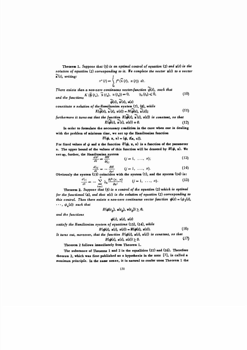
Theore. 1. Suppose tAat (3) is em optimal con.trol of equation (2) ond x(t) is the

solution

of equation (2) corresponJing to

it.

We complete the

vector z(t)

to

a

vector

~ t ) ,

writing:

t

.1,11

(I)

= r II

(I)) tlt,

to

There exists ,hen (J non-zero continuous vector-function

t/J{t),

such that

cl

r. • K (+ (Itt), i (t

u

),

It

(to») == O. 'tu (to) 0,

an tne Junctwns

'

,....,

1/J{tlt s : e ) ~ u(t)

constitute

a

solution

of

the

Ha;miltonian

system (7), (8),

while

'V

K{t/J{t}, x (t), u(t)) =

N(t/J{t),

x(t»;

urthermore

it

turns out that

the

function

K(t/J{t»)

x

(t), u(t») is constant, so

that

4'\

K ~ t , x

(s),

u(t» :=o.

(12)

In

order to formulate the

necessary

caodition in the

case

when

ODe is

dealing

with the problem of

miDimum

time, we set up the Hamiltonian function

H(t/J, s, u) = <rp, b, u».

For fixed wInes of 1/J and x the function H(t/J, x, u)

is

a

fuoCtiOD

of

the

parameter

u. The

upper bound of the values of this function

will

be denoted by 11<

s:).

We

se t

up, further, the Hamilt9DiaD system

d:t

J

all

il

=

au,

• J

d

o

,,- oH . (I

L

)

_ J

( /= J ,

. . .

,I1).

(/1 fix.'

Obviously

me

system

(13)

coincides with

the

system

(1), and the

system

(14)

is :

n

\

t a/

k

(s .

If)

d I

= - -.; Ylt ax'; •

Theorem

2. Suppose that (3)

is

a control

of

tAe equation (2) which is

optimCJl

for

the functional

(4),

and

tAct

s(t) is

the

solution of equation (2) corresponding to

chis

control.

Then there e%ists a non-zero continuous vector function t/J{t) -= (r/J1(')'

• • • ,

'

n

(t»

sucb.

tnat

and the

functions

t/J{t),

x(t), u(t)

sou« fy the Hamiltonian system of equations

(13), (14), while

H(t/J{ ), s(t), u(&») - M(t/J{t), s(t»). (16,

It

turns

out, moreover,

,hat

the funct ion H(t/J(t), x(t ), u(t) is

constant,

so

that

H(t/J{t),

:I:(t),

U(l»

o. (11)

Theorem 2 follows immediately from Theorem 1.

The substance

of

Theorems

1 aDd 2

is

the

equalities

(11) and (16). Therefore

theorem 2, which was first published as a hypothesis in

the

Dote [1],

is

called a

ma imum

principle.

la the same sense,

it

is natural to coofer UUOD Theorem 1 the

130



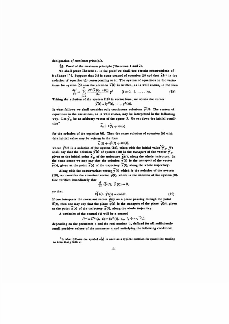
designatioD

of mo imu11I

principle.

§3 .

Proof of the maximum priDciple (Theorems 1 and 2).

We shall prove Theorem 1.

In

the proof we shal l ase

certain constructions

of

McShane

[5].

Suppose

that

(3)

is

some

coouol

of

equation

(6)

and that

is

the

solution of

equation

(6) corresponding to

it . The system

of

equatioDs

in

the varia

tiODS for system (5)

Dear the

solution

x(,)

is

written, as

is well

known, in the form

• 11 , ....

dyl _

aI' (x (I).

It

(t» j

0

d

t

-

L.J ax} y (i = , -J. ••• , n 0

;=0 ·

WritiDg the

solutioa

of-the

system

(18)

in vector

form,

we obtaia the vector

y(t)

== (yO{t), •• •

, rll(t»).

In

what

follows we

shall

consider

only

continuous

solutions

y(,).

The

system

of

equatiens

in the variations,

as

is well known,

may

be

iaeerpreeed

in the following

way. Le t Yo be aD arbitrary vector of the space S. We

set

down

the initial eoadi

tioa

X

o

+aYo -i-

ao

(a)

for the

solution

of the equation

(6).

Thea the same solution of equatioD (6) with

this init ial value may

be wri tten in the form

'i (t) +ay(l) -:-

aO

(3),

where y(t)

is

a

solution

of the

system (is), taken with

the

initial

value

yo. We

shall say that the solution y{') of system

(18)

is

the

'ransport of the vector YO

given at the init ial poiat 0

of

the

trajectory

~ t ) t

along

the

whole

trajectory.

In

.same

sense

we may

sa y that

the

solution r(I) is

the traDsport of

the vector

f(r).

given

at

the

poiat of

the

trajectory

aloD,

the

whole

rrajectory.

4 \,

Along with the

contravariant

vector

y

(I) which is tbe solution of the

system

'

18). we consider

the

covariaot vector .pcl), which is the solutioa

of

the system (8).

ODe

verifies

immediately that

d

- -

d:i

~ t ) , )'

(t» =

0.

( 19)

so that

~ t ) ,

y t»

=

canst.

U

one interpre ts the covariaDt vector .p(e) as a

plane

pass iDg through the point

~ t ) ,

then

ODe

may

say

that

th e

plane is

th e

ttaDSpon

of

th e

plane

~ r ) t giveD

at the

point of

the trajectory ~ t ) t aloDI the

whole

trajectory.

A

variation

of

the CODttO

(3) will

be

a

control

U*

=

U*

(a, el)

=

(u*(t),

t

u

'

t1

+

(Sz,

~ u ) ,

depending

00 the parameter e and

me real

number

a.,

defined for

all

sufficiendy

small posit ive values

of the parameter

e and satjsfyiag

the following

condition:

*10what

(0110w8

the symbol o(€ ) is used as a typical notation for quantities teading

to zero alODgwith

e.

131



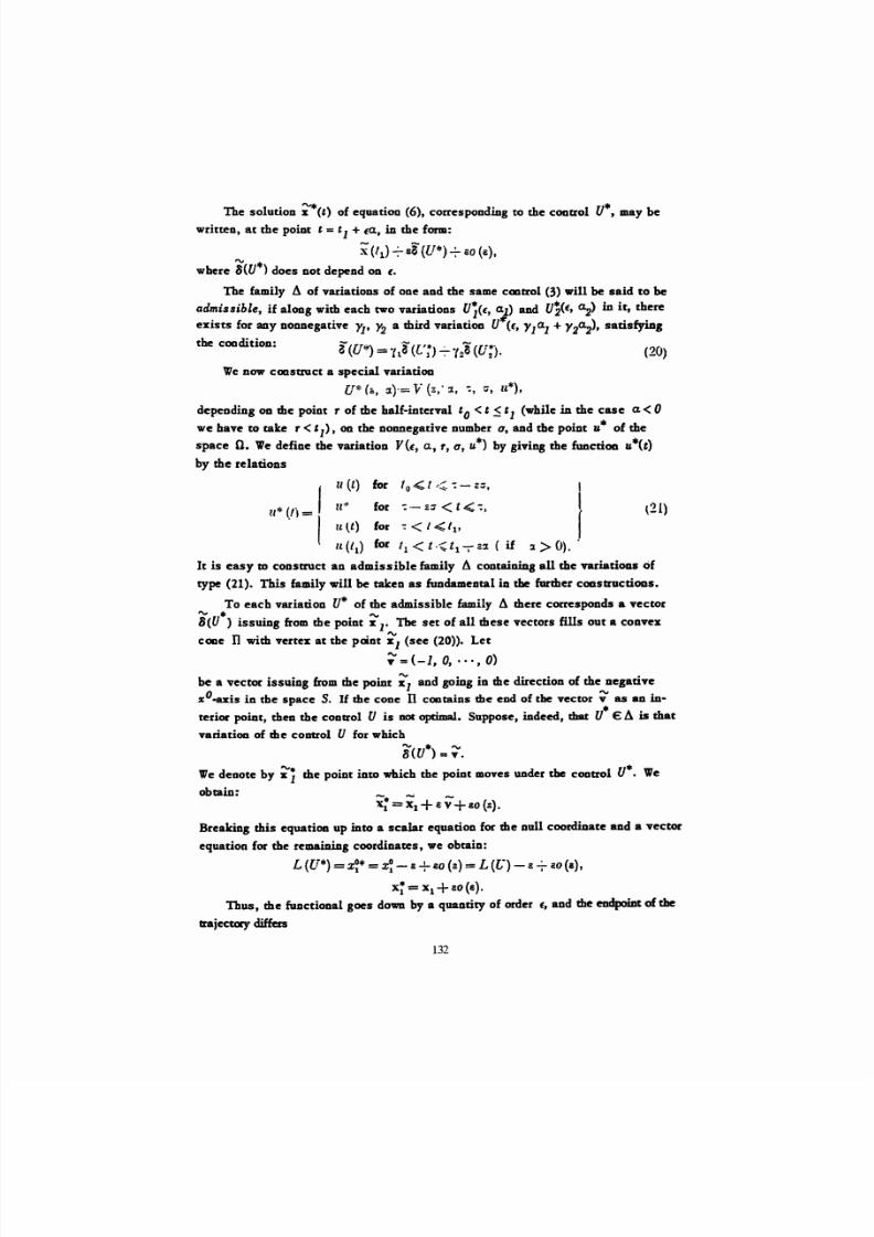
The

solution

i *(t)

of

equation

(6), corresponding to the

coetrel

U·,

may be

written, at

the

point t = t

1 +

fa ,

in

the

form:

X

/

1

) -: - sa

(ll*) +

so (e).

' *

here

8(U ) does Do t

depend

on E.

The

family

A

of variations of

one and

the same

.cmtrol (3) wil l be

s aid to be

admissible, if along with

each

two

variations U ~ « , al l

and

U ~ E t 0-

2

)

in it ,

there

exists for any DODnegative }fl Y2 a

third

variatioD U*(r,

Y1

o,1

+

y

2

0-2) '

satisfying

the

cooditioo:

iW ')

=-t;aw;)

71;B(U:). (20)

We

DOW

ceastrace a

special

variatioo

U* 1; s , ~ , -=,

e, u*).

depending

00

the

point

r

of the

half-interval

to

<

t

t1

(while

in

the

case a.

<

0

we

have

to cake r

< t

1)' on

the

nODnegative

Dumber 0 , and

tbe

point u·

of

the

space O. VIe

defioe the

variation Y(i , a,

r a, u*)

by

giving

the functiOD

u*(t)

by

the relations

(21)

II (t) for

u* (Ii =I

I

ll-='

fo r

- : - :£ :1

<

t -c

:,

I

ltV) for -:< 1< /

1

,

I

II (i

l

) for /1 <

t

t

1

7

( i f :1

>

0).

It is

easy

to construct an admissible family 11

containing

al l the variatioas of

type

(21). This

family will be taken as

fundameotal in

the

farther

cODstrucUODS.

To each

variation

U·

of

the

admissible family I

there corresponds

a

vector

.

B(U )

issuing

from the

poiat

x

r

The

set

of

all

these

vectors fills

ou t

a

eeavex

ceae

n

with

ver tex a t the point

(see

(20». Le t

~ ==

(-1,

0,

•. .

, 0)

be a vector issuing from the point aod going in the

direction

of

the

negadve

s°-u:is in

the

space S. If the cone n COOtai05 t he cod of

th e vector; ' as

aD in

terior

point, thea the control U

is

DOt optimal. Suppose, indeed,

that

U* € A

is

that

variation

of

die

control U for which

* '

(U ) = v .

We denote by the polat into

which

the

point

moves UDder

the

control U*. We

obtain:

Breaking

this

equation

up

into

a

scalar

equation

for

the

Dull

coordinate

and

a

vector

equation

for the remaining coordinates, we obtain:

L(ll*)

= x ~ *

= -

a

+eo

(a)

= L(L·) -8720(1),

X ~ = X l + a o e .

Thus,

the

functional goes

down by a

quantity

of order f,

and the endpoint

of

the

erajectory differs

132



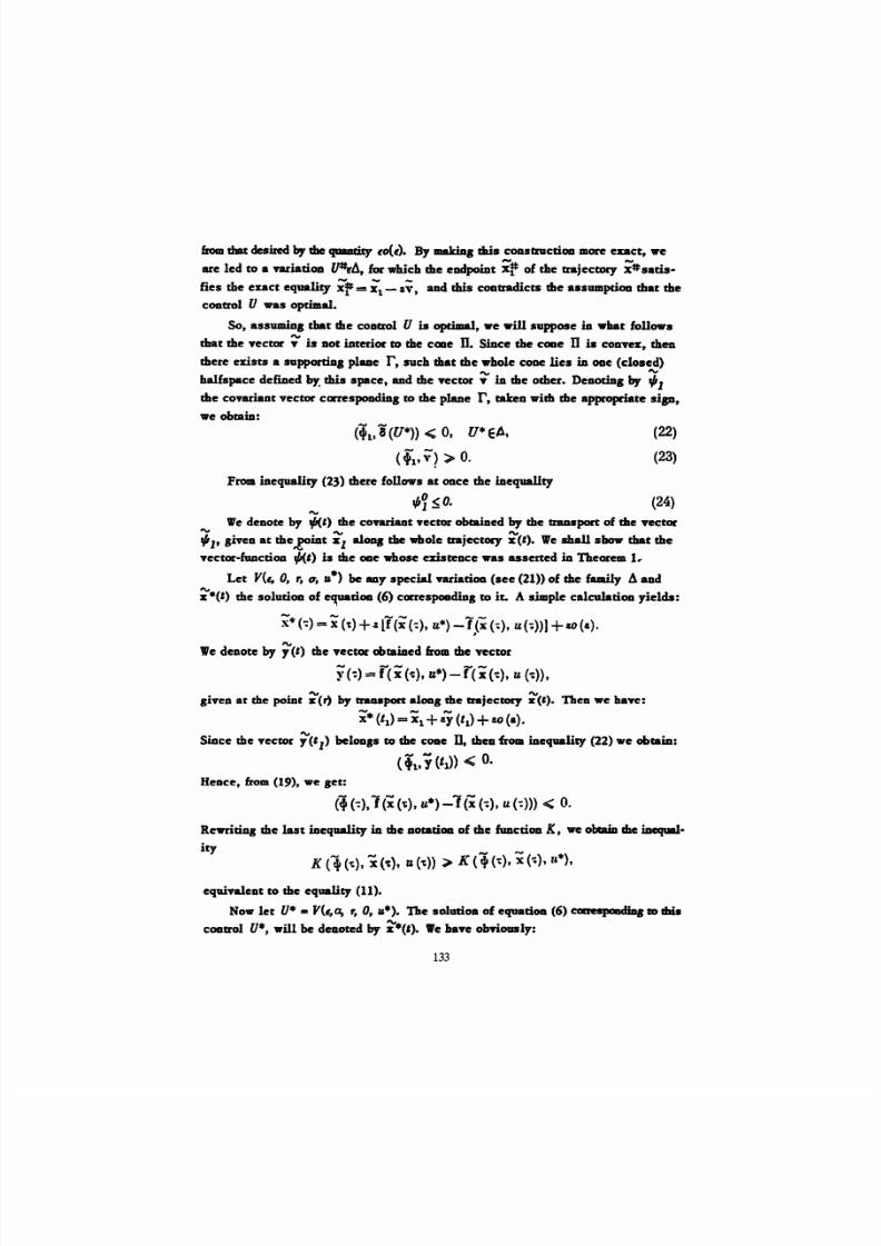
from

that desired by die qaaauty

£0(£).

By maida, dais

CODStruction more e:mct,

we

are led to a varia tion

lJ#rA,

lex whicb the eodpoiDt xf 01the trajectory x#sads

fies the

euc t

equality i f == ;1- av, aDd this coatradicts the assamptioD that the

coatrol

U

was

optimal.

So,

assumioa that the

coatrol

U is

opdmal, we

will suppose

ia

what

follows

that the

vector

~ is Dot iAterior to the eeee D. Since the eeae n

is

CODvex, thea.

there

exists

a suppordDI

plaac

r, such

tbat the

whole CODe

lies in ODe

(closed)

halfspace defiDed bY . this space. and the vector ;- ia the

other.

DeaotiDg

by

~ 1

the covariant vector carrespoodias

to

me plane

r,

taken with tbe

appropriate

s ip ,

we

obtain:

(+1 i (U*» <; 0, u* eAt

(+I

t

:>

o.

(22)

(23)

From inequality

(23)

there follows

at eeee

the iaequa1ity

SO. (24)

We denote by tP< )

the

c:ovariaat vector

obtaiaed

by

the

traII.port of the

vector

~

l siveD

at the. r i a t

Sl

aloug the whole

trajectory

set). We

shan

sbow that the

vector*fuacuOJl

t/J(,)

is the eee

whose

eDsteace

was

asserted il l

Theorem 1..

Le t Y{4

0,

r, 0', II

*)

be

aay

special ftfiarioo

(see

(21) of the

faaUy ~

aDd

z ·(t) me solutioD of e ~ u o (6) correspoadial to it . A simple caleulatioa yields:

x * ~ ) = i t ) + . i l x ~ ) ,

u*)-f(X(-;),

u(-;»J+&o{a}.

,

We denote by

yet)

the

vector

obta.iaed from

the vector

y

=f(

i

u·)

- rei (-e),

u

(-;»),

given ar

the poiDr

by

traasport sloaB

the trajectory

~ e ) .

Thea

we

have:

x*

(t

1

) = Xl

+21 (t

1

) +.£0 (a)

Since

the vector

Y('l)

belODls

to

the coae

D,

thea frOID inequality (22) we obtain:

(+lt1 «» -c

o.

Heeee, from (19), we sec:

<t

(-:),1

(i

(,;), u*) -1

(x (-;),

u

(-:») <;

o.

Rewritias

the

last

inequality

in

the

aotatiOD

of

th e

function

K,

we obcaia the

ioequa1

it y

equivaleDt to the

equality

(11).

Now le t

U* - Y f ~ a

0,

u·).

The

solutio.

of equatiOll (6)

caaespaadiD, ID Ibi.

coatrol

U*,

will

be

deaoted

by

i *(,). We have

obTiously:

133



where

'

ince the vector 8(U*) belongs to the ceae TIt then &ominequality (22) we obtain:

:1

<+1 1(i

l

.

u (t

1

» ) -c o.

Taking

account of

the

fact that a.

is

an arbitrary real number,

the last

inequality

is

possible

only UDder the cooditi01l

1(x

l t

u

(t

1

»)== 0,

Le.,

ooly for

(25)

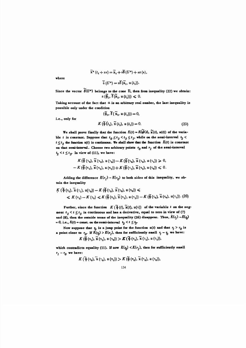
We

shall prove

finally tha:t the function

K(I) K ~ t ) ,

u( » of the

varia

ble

t is CODStaDt.

Suppose that to '2

<

's

t

r while oa

the

semi-interval

<

t the fuocti.oa u<t> is cmtinuous. We sba1l show that the

functioa

K(t) is CODstant

on

that semi-.iotenal. Choose two arbitrary poiots 0 IUld '1 of the semi-interval

t

2

<t 5'3- In view of (11), we have:

K <+ (0:

0

) ,

i

('to), U (0:

0

» - K ~ t o ) , i

~ o ) ,

U

('t

1

» > 0,

-K ~ t l ) x('C

1

),

U

(1i

1

»+K

(+('=1)'

X('t

1

), It(-:o)) <:

O.

Addiag the difference K( l) -

K(,O)

to both

sides

of

this

inequality, we ob

taia

the inequality

K <1

~ 1 ) X

(-:1)'

u(-=o) -

K ~ ~ o ) ,

X( ;0)' U ( eo»

<;

-c K ('t

1

) -

K (':0) <:K

('t

1),

i (t

1

),

U ( =1» ~ K (+ ('to), i (to), u('t

1

»·\26)

Further, since the funcu9D K (1 (t), x(t)t of the variable t 00

the

seg

ment

2 <, is

continuous and has a der ivat ive, equal to zero

il l v i ~ w

of (7)

and

(8), then the outs ide terms of the inequality (26)

disappear.

Thus, K( i)

-K('Q)

z::

0,.Le., K(t) = coast. 011 me selDi-iatenal ; <

t

S

Now suppose that '0 is a jump point for the fuacaoa a(t)

and

that

'i

> 0

is

a

point

close

to

'0.

If

K(ro)

>

K( l)

then for sufficiently small

'i -

'0

we

have:

K

(+ ~ l ) i

(1:

1

), It > K <l

(1:

1

),

i

(-=1)' u ~ 1 »

which coaaadic:ts equality (11).

If

DOW K(ro) <

K( l)

then for sufficieDdy small

'1

- 0 we

have:

K ~ t o ) , ;

(0:

0

) ,

U ('t

l

»

> K ~ ~ o ) , i ~ o ) , u ( =0»'

134



(27)

(i == 1, .... ,

n),

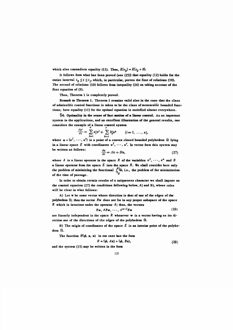
which also cODtradicts equality (11). Thus,

K(,O) - KC,O + 0).

It

follows

fromwhat

bas

been

prmcd

(see (25»

that

equality (12) holds

for the

entire ioterval 0

t

l

which, in particular, proves rhe

first

of

reladoas

(10).

The second of relations (10) follows &om iaequality (24)

Oil

cakiDg

aceoaR : of the

firs t equatioD of (9).

Thus, Theorem 1 is completely proved.

Remark to Theorem 1.

Theorem

1 remaiDs

valid

also

in the

case that the

class

of admissible coetrol functioDs

is

takeD to be the

class

of

measartJble

bounded func

tions;

here

equality

(11) for

the

optimal

equation

is

satisfied

almost

everywhere.

§4. Optimality in the sease of fast aaott_ of • liaear eGatrol. As an i.partaat

system in the

applications,

and ao excetleDt

illustration

of the general results, ODe

ceaalders the ezample of a

linear coatrol system

n ,.

%1 ~

~

lit = ~

aJx'

+ ~

;=. l l=f

where a = (1£1

• • • • •

u')

is

a poiat of a convex closed bounded polyhedron n

lying

in a l inear space E with coordinates .1 , . . . , u,'. In vector form this system may

be

written as

follows: dx

= ~ 1x+Bu

dt

t

(29)

where

If is

a

linear

operator in the

space

R of the

variables s1 ,

. .• ,

SR

and B

a

linear

operator from

the

space

E

into

the

space

R.

We

shall

consider

here

ooly

th e

problem of miDimiziag the fuDcuonal ~ l t Le., the p r o ~ m of

the

minimizatiOll

of the time of

passage, 0

In order to obtain certaiD results

of

a uaiqucness character we shan impose OD

the control

equatiea (27) the

conditions followioB below, A) and B), whose

roles

will be

clear in what follows:

A)

Let w

be some

vector

whose directioD is

dlac

of

oae

of

the edges

of the

polyhedroa 0; then the

~ e c t o r

B. does Dot li e in any proper

subspace

of the

space

R

which is invariant under the operator A; thus, the ~ e c t o r s

Bw, ABw, ..... tAn-lB.

(28)

are

linearly

independent in the space R whenever is a

vector

bavin,

a s its

di

rection one of

the

directions of

th e

edges of

the

polyheclraa

O.

B)

The

origin of coordinates of the space E is aD iDteriar poiDt of tbe polyhe

droa O.

The mactioD H(J/J,

s , . )

io our case bas the form

H = (t/J, Ax) + < , Bu),

and the

system

(15) may be wri tten in the form

135



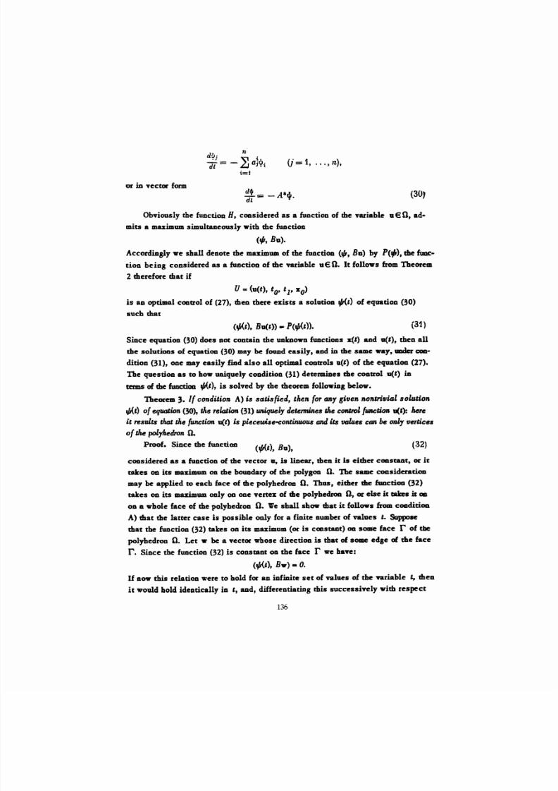
(j

==

1, . . . , n).

or in

vector

form

=

(30)

Obviously the function H, coasldeeed

as

a function of the variable u

en,

ad

mits a maximum simultaDeously with the function

(.p,

Bu).

Accordingly we

shall

denote themaIimWD.ofthefuocuoo(.;.Ba) by P(t/I), the

fUDc:.

tioD

be

ing

considered

as

a

functioD

of

the

variable

uen.

It

follows

from

Theorem

2 therefore that

if

U

==

(a(t), to t l

'0)

is aD opumal cODuol of (27),

thea there exists

a

solatioa

f/1{e) of

equation

(30)

such

that

<¥At),

Bu(&)} -

P(¥At)).

(31)

(32)

(¥AI),

Ba),

Since equation (30) does Dot contain the unknown functions set) and 0 (' ), th en all

me solutions of equauoa (30)

may

be fouad easily, aad in the same

way,

UDder coo

dinon (31), one

may easily

find

a lso a ll

optimal cODttols

aCt)

of the equation (27).

The question as to how uniquely condition (31) determines the control u(t) in

terms of the function

¥At),

is

solved by the theorem followillg below.

Theorem

3.

If

condition

A)

is satisfied, then for

any

given nontrivial solution

VA.t)

of equation

(30), Merelation (31) uniquely

determines

tAe co1JtlOl function 11(1): here

it results that Me function u(t) is piecewlse-continuous

and

its fJdlues can be only vertice.

of the polylaetlron

n.

Proof . S ince

the function

coas idered as a function of the vector a,

is

linear,

then

it

is

either COJlsmat, or it

takes

OIl

it s manmum

OIl

the

bouodary

of the polYBOD O. The same

colIsideradOD

may be applied to

each face

of me polyhedron

O.

Thus, either

the

fuacuoa

(32)

takes 011 it s

mazimumonly

OD one

vertex of

the

polyhedron

0,

or

else

it cakes

i t OIl

OD

a whole

face

of the

polyhedron O.

We shall show

that i t

follows from

CoadiUOD

A) that

the

latter case is

possible

only

for a f in ite number of values t: Suppose

that

the

fuoctiOD

(32)

takes

o.a

it s

muimum

(or

is

coastaat)

OD

some

face

r

of

tbe

polyhedron O.

Le t

- be a vector wbose direction

is

that of SODle edge of the

face

r. Since the functioD (32) is constaDt on

the

face r we ba'Ye:

(y,(t),

Bw) -

O.

If

DOW

this

relation were to

bold

for au inf in ite set of values of the

variable

t; mea

it would hold identically in , and, differentiating this successively with respect

136



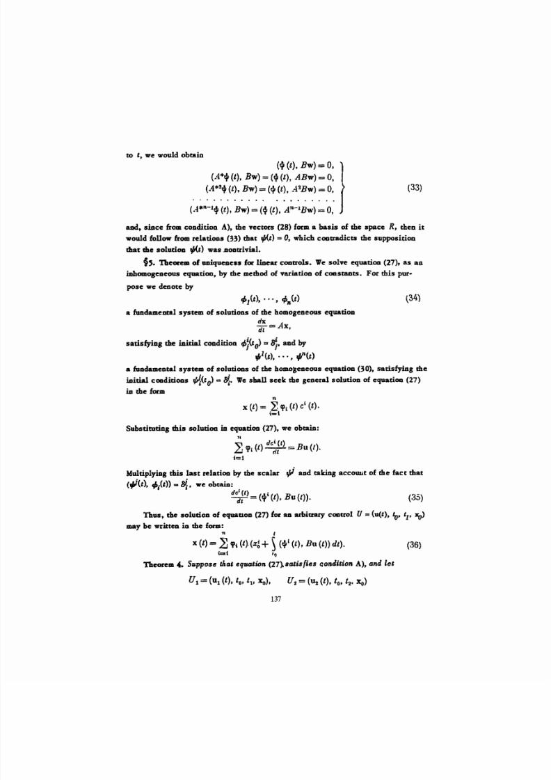
to

It

we would obtain

(4' (t), Bw)=0, 1

(t),

Bw)

=

(cf1

(t), ABw)

=0,

(.4*2+

(t), Bw)

= (cf1 (t), ..4 Bw) = 0, f

. - t . n ~ l ;

(t),

~ : : :

(+ (t), ~ ~ - ~ B ~ ~ · O

(33)

(34)

and,

siace from conditioo

A),

the vectors

(28)

form a

basis

of the

space

R, then

it

would follow

from relations

(33)

that t/J{t) =0,

which

contradicts the supposition

that the

solutioD t/J{t) was .noDtrivial.

§5 .

Theorem

of

aaiqueaess

for

lioear

cODuols. We

solve

equatioa (27),

as

all

iDbomogeaeous equation, by the method of variation of CODstaDts. For

this

pur-

pose

we

denote

by

rpl(t), • · . , tP

Ta

(t)

a fuodameatal

system

of

solutions

of the homogeneous

equation

dx A

Ci't = x,

satisfying the initial condition t I > ; U o : : r ~ . and by

,1(I.), •• •

,

,7I(t.)

a fundameDtal system

of

solutions of the homoBeneous equation (30), satisfying the

iaitial coaditioas

tP{(t

O

)

~

We

shall seek the

general solution

of

equation

(27)

iu

the

form

n

X (l) =

fPi (t)

c

i

(t).

i-t

Substituting this solution in

equation (27), we

obtain:

't

dc

i

el)

£;,J <Pi

(t)

cr;:- = Bu (/).

i=1

MultiplyiDI this last

relation

by the scalar

.pi

and

taking

accouut

of

the

face

that

(t J(t),

~ i t » ::a we obtain: .

t l c ~ t

= ('l'i

(t),

Bu

(t». (35)

Thus, the

solution

of

equauoD

(27) tor aD arbitrary control U =

(U(I), '0* t

I

, XO)

may be wri tten in the form:

'n t

X (t) = ,dt). + ('l'i (t), Bu (t) dt). (36)

=1 II)

Theorem 4. Suppose tho' equotion (27). .atisfies l;on4itioll A), and le t

137



(:iH)

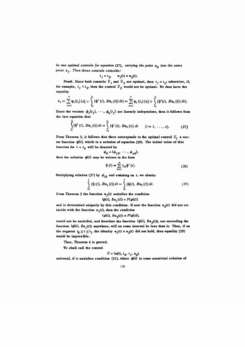
be two optimal controls for equation (27), carrying the point

X

o

into the same

point

S I

The ,

these

controls co;,ncide:-

i :

t

2

, U1(£)

5:

u

2

(t).

Proof . S ince both controls Uland

U

2

are optimal, then t

1 •

t

2; .

otherwise,

if,

for example,

t 1

<

2'

then

the control

U2

would Dot

be

optimal.

We

thus

have the

equality

'1

1 n. I i

Xl = ,.(1

1

)

(x:

-t-

(I), ]JUt (l)) d/) - 'i

(ll) (If/;(t), BU2

(l)) dl).

;= 1

10

i= 1 It)

Since

the vectors tfJ

j

(t

1

).

' •• , rPn(t

1)

are

linearly independent, then it

follows

from

the

last

equation

ma t

11

I i

(If/i (I). lJudt» dl= (lJIt

(I). (I»

dt (i

=

J

•••••

11). (37)

0

fu

From Theorem

3, it

follows

that

there corresponds to the optimal control

U

j

a

vec

tor function

1/1< ),

which is a

solution

of

equation

(30).

The init ial value

of this

function

for t = to

will be denoted by

tPO=(t/J10' • • • • .pnO);

thea the

solutioa

.p{t) ma y be written in th e form

n

tfI (1)

=-

f 1 i C l ~ i (t).

i= l

Multiplying

relation

(37)

by

.piO

and

sUliuDing

011

it

we

obtain:

I

f

(4' (I), Budi)) cit = Bu (I}) dt.

10

to

From Theorem

3 the

funct ion a

1(1,)

satisfies the

condition

<1/I(t), Bo

1

(t» == P{f/At)

and is determined uniquely

by this

coaditicm. I f

DOW the

funcuoo u

2

(t )

did

not co

incide with the

functioD

U

l(t),

thea

the

coaditioD

(y,{e),

Bu

2

(t » e P(¢<t»,

would no t be

satisifed,

and

dJerefore

the function (.p{t),

Bu

2

(t » , oot exeeedleg the

function (¢<t), Bul(l» anywhere, will on some interval be less thaD

it .

Thus, if

OD

the segmeot

to

.:S

t I the

ident ity u

let)

==

u2

(t )

did Dot bold,

thea

equality

(39)

would be

impossible.

Thus, Theorem 4 is proved.

We shall call the

CQDtrol

U

= (u(t), 0' t l 'SO)

extremal, if i t satisfies condition (31), where 1/1<,) is some

nODtrivial

solution of

138



equatioa

(30)-

Ia order to fiad al l optimal cODuols carryiD. the poiat So Ieee me poiat

Xl

oae

may

Bad first

al l

extremal controls carrying the point X

o

into the poillt Xl aDd

thea

chose &omtheir

Dumber

the uniqae one

which carries out this passage

iD the

shortest time. The quesdOll arises, as to whether there lDay be

several

extremal

CODUO s

carryiDg the point X

o

into the point

E

l

- 'Generally speakhlat there may

be

several of them. The theorem followiDg below indicates aD important

case

of wi·

city.

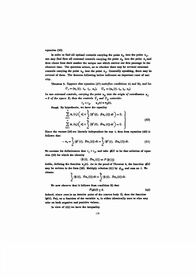
Theorem 5.

Suppose

1uJ

efJUtJtiora

(27)

satisfies contlition.

A) GntI B), GDIl

Ie'

U

1

= (u

1

(t),

to'

t

1 t

xo), U

1

== (U2

(t), to,

t i t xo)

be , ,0 es ernGl

ccmtrols,

otJlT'1iDg

the P?ill' i to

,lie origin

of'coortli7IG'es

Xl

.. 0

of Uae spaee

R;

then tAe control. U

1

tJDl U2

comella:

'1 == '2 '

Dlft} =

Proof. By bypothesis, we have die equality

fa

h

~ CPi. (11)

(

+ (t

i

(I), Bill (t» dt) =

0,

~ t

~

4 ~

cpdls) ( x:+

(t

l

(I),

BUs (l» dt ) = o.

1=1 to

Since the

VectorS (34)

are linearly iDdependeat fer auy

t,

then &omequatioa (40) it

follows that

t l

.

- X

o

=

(t

i

(I),

BU

I

(l» dt = ( fIi

(I),

BlIa

(l»

dt.

1o to

(41)

We assume

for

defiaiteaess mac '1

>

'2 '

aDd take

fI...')

to be that solatioDof equa

dO D (30) for which

me

identity

(4' (t), BU

1

(t» == P (t (t»

holds, defiaiD.

the

fuactioD 8

1

( ') . As ia the proof of Theorem 4, the fuactioD ;<,)

lDay be wri ttea io

the

form (38). Multiply relatioD (41) by

tfi

iO

aad sum on

t.

We

obtaia:

We

DOW observe

mat

i t

fonows

frDlD

cOIIdiuoa

B)

that

2: o.

Indeed, siace zere is

aD

iaterior point of the CODvez body

0, thea

the fuDctioa

~ , ) , Ba), as • function of the variable

a,

is either

ideadeally

aero or

else

may

take on both

nesaave

aad posidve ftlues.

In view of (42) we have die inequality

139



Is

(HI),

B U l t » d l ~ <+(t), B ~ { t d t .

to

Hence,

just

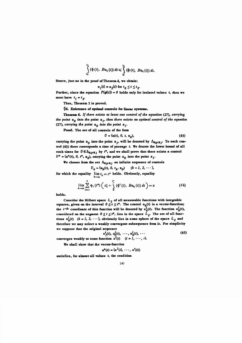
as in the proof ofTheorem4, we obtain:

DZ(t) == u2( ) for

0 t 5'2

Further, siac'e the equation P(tfi{,» - 0 balds only for isolated values t then we

must

have '1 • r

Thus, Theorem

S

is proved.

96.

Ezisteace of

opcimal

cOIIU'ols

for liaear syatelDS.

Theorem 6. If there

esisu

at

lea one

con rol

of

the equation

(27),

carrying

'h e point

Xo

into

llae point

S l

thera

tAere

esisu GI l

optimal control

of

the

B'lutJeloT.

(27),

carryin& dae

point.

So

into the poin' s

1.

Proof. The set of al l

CODtrois

of the form

U

=

(u(t), 0,

t, sO), (43)

carrying the

point SoD

iDto the point

'S.l'

will be denoted

by AZO'Zl-

To

each coo

uol

(43)

mere

eorrespoads

a rime

of passaIc s: We

denote

the lower bound

of all

such

times for U € Aso.z1 by t*, aDd we shall prove

that

there exists a

control

U* • (0*('), 0, . , 'SO)' carrying the point

Zo

into the paiat z 1-

Wechoose. &om the

set lz.O'Zl

an

infinite sequence of controls

Uh

== (u,(t),

0,

i

sO)

(It: = 1, 2, .. · ),

for which the equality lim

tit

= t*

holds. Obviously, equality

k

......oo

holds.

n i.

lim crt (t*) +-

(t), BUIe «»

dt)

=

x

I ~ - + o o 1=1 0

(44)

(45)

Consider

the

Hilbert space

L 2

of

al l measurable fuactioDS with

integrable

squares,

li\ 'ea

011 the iaterval 0 t*. The

cODuol

Dlet)

is

a

vector-macnoD;

the

i-

ch

coordiaate of

this

function will

be

denoted

by ut<t).

The function 1< ),

considered on

the

sepcDt

0

oS'S

t*,

l ies ia

the

space

L 2.

Th e

set of aU fuac

tiODS

U1e£) (Ie -1 ,

2

••••

), ob\'iously lies in

some

sphere

of the

space L2 and

therefore we

may

select a

weakly coover,eDt subsequence· from it .

For

simplicity

we

suppose

that

the

oriliaal

sequeace

i

uj< ),

'4Ct),

•••, a

Ct),

•••

converses

weakly to some

functioD

a

i

(, )

(i -1 , ••. ,

r).

We

shall

show

that

the vector-function

u*(t) - (u

1

(t), •• • , u'(t»

satisfies,

for almost al l

the coadition

140



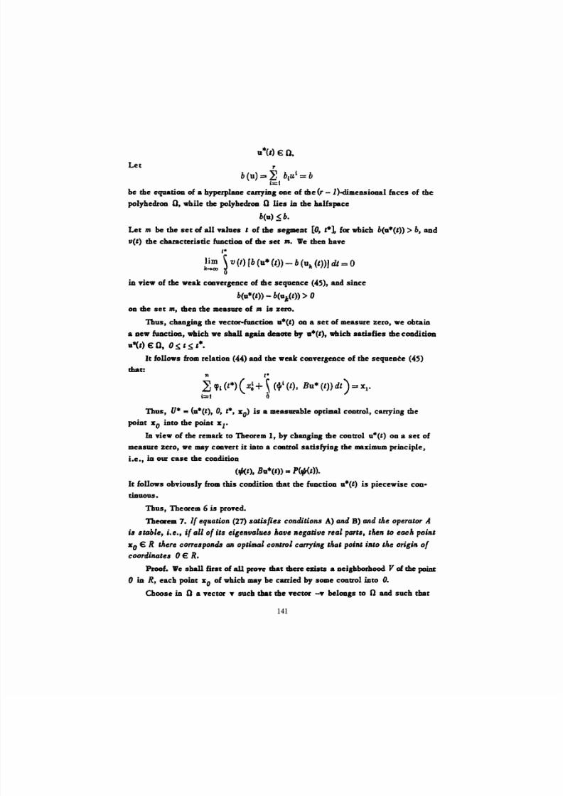
Le t

u*{t) € o.

T

b(u) := I biu

i

=b

i= f

be the

equauou

of a hyperplaae carrying

ODe

of

me (r - l)-dimeasioaal

faces of the

polyhedron

0, while

the polybedroa

0 lies il l the halfspace

b(a)

s b.

Le t m be

the

set of al l values t of the segmeJlt [0, '*1 for which

b(a*('»

> b, and

11(1) the

cbaracrerisdc

function of

the set m. We thea

have

,.

lim

v

(I)

[b

(u*

(I)) -

b

(U,.

(t))J

dt

=

0

k-.CIO

0

in

view

of the

weak

cCDvergence of me

sequence

(45), and

since

6(1I*(t» - b(uk(t»

>

0

OD me

se t m, then the

measure of

III is zero.

Thus,

changing

the vector-functiOD

8*(t)

00 a

set

of measure

zero,

we

obtain

a aew function, which we

shall

agaiD.

deaote

by

a*(t),

which satisfies me

condition

lI*(t) € 0,

0

S,

t S , •.

It

follows &om

relation

(44) and the weak convergence of

the sequeDce

(45)

that:

11

to.

Cfi

(t·) (

x: + (+1 (t), Bu «»

dt

)

= xl'

i= t .,

Thus,

U*

= (1I*(l),

0, t*,

'So) is

a

measurable

optimal

eentrel,

carryiog the

point :EO i nto the point x

r

IDview 01 the remark to Theorem 1, by ChBDliug the

coatrol

u*(t)

OD

a

set

of

measure zeee, we may convert i t into a coottol satisfying the maximum priaciple,

Le.,

ia our

case

the

condition

(r/J(t), BU*(I) =-

P t / A ~ »

It

follows obviously fromthis COaditiOD that the fuocdoD u*(t)

is piecewise COD

tinuous.

Thus,

Theorem 6 is

proved.

Theorem 7. If equation (27) satisfies condieions A) antiB) antI the operator A

is

stable,

i.e.,

if

all

of

it s

eigenvolues

Aave

negative

reol

parIs,

then

to

each point

So

€ R

ther« CO e8pOnU tJIJ oplillltJl

conlrol carrying

tha

poin' into the origi

of

coortliRtJles 0 €

R.

Proof. We shall

first

of

all

prove

that

there

exists

a aeighborhood

Y

of the

point

D in R, each

pohle

'So

of which

may be carried

by

some

control

into

O.

Choose in 0

a

vector

y

sucb that the vector -y beloags

to

I}

and

such that

141



the vector

b =

By

does Do t

belong

to

any

proper

subspace

of the

space

R which

is invariant

under

the

operator

A. From

coaditioas

A)

and

B)

it

follows that

there is such

a

vector

v.

Fo r a sufficiencly

small positive

(

the

operators A.

and e-

f A

have eeiecideet invar

iant subspaces, and therefore the vectors

e-;Ab. e-

2IAb ,

. . .

,

e-

l1 l Ab

are linearly Iadepeadeae,

Le t x(t)

be

auy

real function, defined on some segment

0

t :s t1 aad Do t ex

ceeding uaity in absolute value; thea

U =

(TX<t),

0, f,l 'So)

is a

coauol

of equatioo (27), and that control carries me point 'So Inee the point

(see

(36»

II.

Xl =

ellA

( x

o

+ e-IAbX

(I)

dt) .

(46)

u

Now we

choose

the function XU), dc:pendiag

00 the

parameters

e'. ...

,

e iD such

a way

that

the

point

(46), which we denote by

1( .0: r. ... ,en). satisfies

me

followiog

cODditiODS:

s'l(O;

0, ••• ,

0) = 0,

and the

Jacobian

•• •

.,

I

1

'n

.1

.1 l

a , ...

t C;) Xo=O

.. . =0,

. . . •

; =0

is

DODzero. Constructing such a

function

X(t),

we

show

that

the equation

Ej(Xo'

• • •

.

e ) = 0

may

be

solved for {1 ,

. . .

J for

al l

values Zo ly..

iag in some

neighborhood

Y

of the origiD

O.

First

of

al l

we define a

mactioa II

(t,

t;

e)

of

the

variable I, 0

5

&

S

t1- where

o

< r <

t1

aad e

is

a parameter. The

fuDCtiOD

a(t,

e as

a

fuDCUoa

of the ftri

able I, is equal to zero everywhere outside die

interval

rr, r+

el,

and OD thac

inter

va l it is equal

to

sigD e. Now pu t

n

X

(t) =

a

(t,

ka,

A=1

A

simple calculation

shows

that

the

point

%l(S.O'

{1,

. .

.

en).

with

this choice of

the function

)((e),

satisfies the stated

caadiuons.

Now

le t

0 be any

point

of the space R. Suppose

that

i t first moves under the

cooaol u(') ii O. Since all eigeavalues of the operator A have negative real parts,

then

after

the

expiration

of some time

the point will

come

into

the neighborhood,

after which, as we baye proved,

It

must be carried

iato

the o r ~ i o of coordinates.

142



Hence, frOID

Theorem 6,

it

follows that there exists an optimal control,

carryioa the

point S.o

into

the origin.

Thus Theorem 7 is proved.

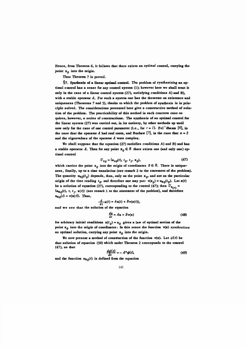
§7 . SJDthesis of a

lia.ear

opdmal control.

The problem of syn,hesizing

aD op

timal ca:alrol has a sense for any

eeatrel

system (1); however bere we sball treat it

oaly in the case of a linear control system (27),

satisfying

conditions A) aDd B),

with a stable

operator

A..

For such a system

one ba s

the theorems

00

ezisteDce

and

uuiqueness

(Theorems 7 and 5), thanks to which the problem of

synthesis is

ha

pria

ciple solved.

The

considerations

preseDted

here

l ive

a cODsuuctive method of solu

tion of the problem. The practicability

of

this method in

each

concrete case re

quires, bowever, a series of cOIlSUUCtiOOS. The syathesis of au optimal coutrol for

the

lioear system (27)

was

carried out, .in

it s eDtirety, by other

methods

up until

DOW only for the case of eee cODuol parameter (I.e., for r - 1). Fe ' dbaum [6], hi

the

case that the operator A had real roots, aDd

Bushaw

[7],

il l the

case that 1& - 2

and the

eigenvalues of the operator

A

were complez.

VIe shall suppose that the equation (27) satisfies conditions A) and B) and bas

a stable

operator A. nen

for aay poiat

So

e

R

there e:asts one (and oaly one) op

timal

control

U

SO

a

(uzO(t), to' t t:

xol, (47)

which carries the point

Zoo

ioto the origia of coordiaates 0 € R. There is uaique

ness, fiDally,

up to a time

traaslation (see

remark 2 to the

statement

of

me

problem).

The

quantity l I ~ O O )

depends,

mus,

only

OD

the

point sO'

and

Dot 00

the

particular

ofigia of the time readiD,

0

and therefore oae may put: v(zO) = uso('a). Le t

x(t)

be a solut ioD

of equation

(27),

correspoodiDg to the

eonteel (47); then

Uz(r) =

(Uzo(t), r, t

I ' a:(r»

(see remark 1 to the

statement

of the

problem), aDd

therefore

us.o(r) =v(x(r». Thus,

. .Lx(t)

• AX(l) + Bv(s(t»),

dt

and we see that tbe solut ioo of the equat ion

...

A:a: + BY(x)

(48)

for arbitrary iaitial coDditioos z('O) =- Xo

gives

a law of optimallDotioD of the

poiot

Xo iato the oriBiDof coorclioates III this sense

the fuactioa v(s)

synthesizes

an

optimal solutioD, carrying

ally

point

'SO

into the

origin.

We DOW present a method of CODSttucUon of the funct ion v(z). Le t be

thac solution of equation (30)

which

UDder Theorem 2 correspoods to die coauol

(47), so that

Jf l.,

-A..

.;ttl,

aad .the funcaoD UXO(t) is defined from the equatioo

143

(49)



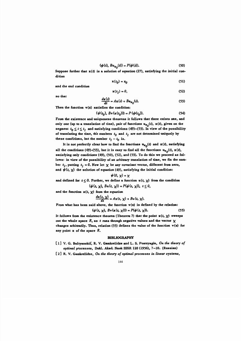
~ e ) , BuKO(t)} =

P(t/1(t».

(50)

Suppose further

that

set)

is a solut ion of equatioD (27),

satisfying

the initial con

dition

(51)

and the end condition

so

that

dx(t)

---;j't :=I As(t) + Buso(t).

Then the function v(z) satisfies the condition:

(52)

(53)

~ t o )

B ~ x t o »

=

P

( (to).

(54)

From

the

existence auld

uniqueness

theorems

it follows

that

there exists one, and

only one

(up to a

naDslation

of time),

pair

of functions u

xO

I,), x(t),

giveD on

the

segmeot

to t So

'1 and

satisfying

conditions (49)-(53). In view of

the possibility

of

ttanslatins the

time,

the

numbers to

and

i are not

determined

uniquely by

these conditions, but the number t

1

-

to

is .

It

is Dot

perfecdy

clear

bow to find

the

functions 8

z0

(t ) and

set), satisfying

al l

the conditions (49)-(53), but it

is

easy to find al l the functions uzo(t),

set),

satisfying only conditions (49), (50), (52), and (53). To do

this

we proc-eed

as

fol

l ows: in view of the

possibility

of

aD

arbitrary

uansladon

of time, we fix

the

num

ber t

1t

puttiDB e

1

=

O.

Now

le t

X. be any covariant vector, different from

zero,

and

f/J

(t. X)

the solution of equation (49),

satisfying

the

initial

condition:

;(0,

X)

= X

and defined for t SO. Further, we def ine a funct ion a(t, X) from the conditioa

(p(t,

X),

Bu(t, xl)=

P(.p

(t, x», t

s

0,

and the function z(t, X) from the equation

h( t , X)

dt tilt Az(t,

X>

+ Bu (t , ){.I.

From

what

ha s beee

said above, the function . (z) is defined by the

relation:

(p(t, X),

Bv(x(t, X» )

• P< 'Ct, X». (55)

It follows from the eustence

theorem

(Theorem 7) that

the

point s(t, 'X) sweeps

out the wbole space R, as , r uns throu,h nega tive values and the vec tor X

chaoses arbiuarily. Thus, relation (.55)

defines

tbe

value

of the function v(x) for

any

point x of the

space

R.

BIBLIOGRAPHY

(1] V. G. Bolty_nski , R. V. Gamlaelidze aDdL. S.

Ponttyasin,

011

the '; eory of

optimal processes, Dokl. Akad. Nauk SSSR 110 (1956), 7-10. (Russian)

[2]

R. V. Gamkrelidze,

On

the

theory of optima,l processes in linear systems.

144



Dokl. Akad. Nauk SSSR

116

(1957),

9-11. (Russian)

[3 ] V. G. BolcyaasJcil, The principle in the theory

of

optimal processes,

Dold. Akad. Nauk SSSR

119

(1958),

1070-1073. ~ u s s i a a

[ .. ] G. A. Bliss, Lectures

011

tAe ctJlculu of tHln_ioM, Uaiversity of ChicaSO

Press,

Chicago, Ill.,

1946.

[The refeeenee in the text is to the Russian edi

tion',

and

probably corresponds to the first few pages of Chapter VII in the

English editioa.]

[

5]

E.

J.

McShane,

Onmultipliers for

Lagrange

problems,

Amer.

J.

Math. 61 (1939),

809-819.

[6] A. A.

Fel'

dbaom, On the design of optimalsystems by meons of pw e space,

Avtomat. i

Telemeh.

16 (1955), 129-149.

(Russiao)

[7]

D. W. Bushaw, E perime7 tal towing tOM,

Stevens Institute

of Technology,

Report 469, Hoboken, N. J., 1953.

Translated by:

j ,

M. Danskin, Jr .

145

Documents

Optimal Regulation Processes