Embed Size (px)
Citation preview
FEDERAL RESERVE BANK OF ST. LOUIS Research Division
P.O. Box 442 St. Louis, MO 63166
______________________________________________________________________________________
The views expressed are those of the individual authors and do not necessarily reflect official positions of the Federal Reserve Bank of St. Louis, the Federal Reserve System, or the Board of Governors.
Federal Reserve Bank of St. Louis Working Papers are preliminary materials circulated to stimulate discussion and critical comment. References in publications to Federal Reserve Bank of St. Louis Working Papers (other than an acknowledgment that the writer has had access to unpublished material) should be cleared with the author or authors.
RESEARCH DIVISIONWorking Paper Series
Optimal Ramsey Capital Income Taxation —A Reappraisal
YiLi Chienand
Yi Wen
Working Paper 2017-024Chttps://doi.org/10.20955/wp.2017.024
October 2017
Optimal Ramsey Capital Income Taxation
—A Reappraisal∗
Yili Chien† Yi Wen‡
October 23, 2017
Abstract
This paper uses a tractable model to address a long-standing problem in the op-timal Ramsey capital taxation literature. The tractability of our model enables us tosolve the Ramsey problem analytically along the entire transitional path. We showthat the conventional wisdom on Ramsey tax policy and its underlying intuition andrationales do not hold in our model and may thus be misrepresented in the literature.We uncover a critical trade off for the Ramsey planner between aggregate allocative ef-ficiency in terms of the modified golden rule and individual allocative efficiency in termsof self-insurance. Facing the trade off, the Ramsey planner prefers issuing debt ratherthan taxing capital to correct the capital-over-accumulation problem. In particular,the planner always intends to supply enough bonds to relax individuals’ borrowingconstraints and through which to achieve the modified golden rule by crowding outcapital. Public debt is financed by labor income tax as it is less distortionary thancapital tax. Thus, capital taxation is not the optimal tool to achieve aggregate alloca-tive efficiency despite over-accumulation of capital. Hence, the optimal capital tax canbe zero, positive, or even negative, depending on the Ramsey planner’s ability to issuedebt. In a Ramsey equilibrium the modified golden rule can fail to hold whenever thegovernment encounters a debt limit. Finally, the desire to relax individuals’ borrowingconstraints by the planner may lead to an increasing debt accumulation, resulting in adynamic path featuring no steady state.
JEL Classification: E13; E62; H21; H30
Key Words: Optimal Capital Taxation, Ramsey Problem, Incomplete Market
∗The views expressed are those of the individual authors and do not necessarily reflect the official positionsof the Federal Reserve Bank of St. Louis, the Federal Reserve System, or the Board of Governors.
†Research Division, Federal Reserve Bank of St. Louis, P.O. Box 442, St. Louis, MO 63166-0442; Email:[email protected]
‡Research Division, Federal Reserve Bank of St. Louis, P.O. Box 442, St. Louis, MO 63166-0442; Email:[email protected]
1 Introduction
The seminal work of Aiyagari (1995) has inspired a large literature. However, despite several
important revisits, such as Chamley (2001), Conesa, Kitao, and Krueger (2009), Davila,
Hong, Krusell, and Rıos-Rull (2012), and many others, the issue regarding optimal capital
income taxation in the heterogeneous-agent incomplete-market economy remains unsettled.
One of the daunting challenges in unlocking the precise mechanisms behind many results
in this literature is tractability and transparency. When models are not tractable, not only
the Ramsey problem becomes difficult to solve, but the proofs also become highly non-
transparent. Consequently, intuitions often get lost and dubious claims may be made.
For example, the competitive market equilibrium in the Aiyagari model (Aiyagari (1994))
may appear to be dynamically inefficient due to excessive accumulation of capital under
precautionary saving motives, which results in excessively low marginal product of capital
at the aggregate. Thus, the modified golden rule (MGR hereafter) is violated and leads
to an aggregate inefficiency. This observation provides the key intuition of Aiyagari (1995)
that the Ramsey planner should tax capital income to restore the aggregate efficiency — the
MGR.
On the other hand, the above intuition for justifying positive capital income tax is
counter-intuitive. By taxing capital income and thus reducing each individual’s optimal
buffer stock of savings, the planner is hampering and even destroying individuals’ ability to
self-insure themselves against idiosyncratic risks. Since taxing capital does not directly ad-
dress the lack-of-insurance problem for households (if anything, it intensifies the borrowing
constraint problem), why would taxing capital always be an optimal thing to do for the social
planner? Or why would the MGR matter to individuals’ welfare more than the need of self
insurance? This question is particularly intriguing since lack of insurance is the only friction
in the economy and hence the ultimate concern for households regarding idiosyncratic risks.
In other words, achieving the MGR through capital taxation does not help at all to alleviate
the primal friction in the model — borrowing constraints, thus using the MGR principle
to justify positive capital income tax regardless of model parameters is not at all clear and
convincing.
1
In short, two margins of inefficiency exist in the Aiyagari model: aggregate inefficiency in
light of MGR, and individual inefficiency in light of borrowing constraints or insufficient self
insurance. Clearly, the aggregate inefficiency is a consequence of the individual inefficiency
(due to externalities of household savings on the rate of return to aggregate capital), sug-
gesting that restoring individual efficiency is the correct way to achieve aggregate efficiency.
Hence, intuition tells us a social planner can improve welfare more likely through addressing
the individual inefficiency problem by relaxing borrowing constraints. Yet Aiyagari (1995)
argues that the social planner should directly address the aggregate inefficiency problem by
hampering individual efficiency, or by sacrificing individual’s buffer stock of savings, regard-
less of model parameters. This conclusion seems dubious and puzzling, for it completely
ignores the trade off between the two margins of inefficiency in terms of benefits and costs.
The goal of this paper is to investigate the trade off between the two types of inefficiency
in a transparent manner. Our contributions are four-fold. First, we construct a tractable
heterogeneous-agent incomplete-market model with closed-form solutions, in which the dis-
tributions of market allocations can be derived analytically. The analytical solution of the
competitive equilibrium simplifies the Ramsey problem dramatically. As a result, the optimal
Ramsey allocation can be derived analytically both along the transitional path and in the
steady state. Armed with the closed-form solutions of the Ramsey problem, the mechanism
and intuition of optimal capital taxation can be seen clearly.
Second, our model has the special property that given an exogenously specified interest
rate identical to the time discount rate, household’s asset demand may remain finite and
in such a case the borrowing constraint never binds for any households. However, if the
interest rate is endogenously determined by the marginal product of capital, then under
sufficiently large idiosyncratic risks, the equilibrium interest rate is always below the time
discount rate, suggesting over-accumulation of capital and failure of the MGR. However,
since the government is able to manipulate the market interest rate through bond supply, we
show whether the modified golden rule holds under the Ramsey planner depends critically
on the government’s ability to issue bond as an alternative store of value for households to
buffer the idiosyncratic risk. In particular, the MGR holds if and only if the government can
issue sufficient amount of bond to completely relax households’ borrowing constraints. Once
2

borrowing constraints are completely relaxed with zero binding probability, the equilibrium
interest rate equals the time discount rate. In such a case, the social (aggregate) efficiency
is achieved, simply because the individual efficiency is fully restored. As a result, there is no
need to tax capital. This result provides a strong rationale for the supply of public debt.
Third, we demonstrate that if the government has limited capacity to issue debt, then
MGR does not hold under Ramsey because individual efficiency cannot be fully achieved.
In such a case, the optimal tax rate on capital income can be either positive or negative,
depending on model parameters. When the optimal capital tax rate is negative, the social
planner is encouraging precautionary saving despite over-accumulation of capital. In this
case individual efficiency outweigh aggregate efficiency for the Ramsey planner, so it is not
optimal to target MGR by tightening household borrowing constraints with positive capital
tax, in sharp contrast to Aiyagari’s (1995) analysis. In other words, there exist situations
where the Ramsey planner opts not to achieve the MGR even if he/she is fully cable of doing
so by taxing capital income.
Finally, we show that there may not even exist a Ramsey steady state if the magnitude of
the idiosyncratic shock is not bounded above and if there is no limit on issuing government
bond. This finding suggests the possibility of having a non-steady-state Ramsey outcome.
Yet the existence of a steady state is a common assumption in the extant literature. Our
finding provides a cautionary note to such a dangerous assumption.
Aiyagari (1995) proves his theoretical results based on a nonstandard feature — endoge-
nous government spending in household utilities, which equalizes all agents’ marginal utilities
of government spending. Aiyagari’s analysis utilizes this nonstandard feature and exclusively
focuses on the efficiency of aggregate resource allocation without worrying about income or
wealth distributions. Yet the main motivation for considering such heterogenous agent mod-
els is precisely that distributions matter for social welfare.1 In fact, allowing endogenous
government spending in our model (the same way as in Aiyagari (1994)) does not change
our results if the distributional effects of government policies are taken into account.
The intuition behind our results is rather simple and transparent. Government bond
1Wen (2015) and Camera and Chien (2014) emphasize the distributional impact of inflation on welfarein incomplete market economies.
3

meets individuals’ demand for precautionary saving without creating externalities on the
marginal product of capital. Hence, by substituting for (crowding out) capital, government
debt can satisfy households’ buffer stock saving motive and, at the same time, correct the
aggregate inefficiency due to over-accumulation of capital. This is why the Ramsey planner
opts to flood the asset market with sufficient amount of bonds to relax borrowing constraints
for all households in all states. As a result, if there is no debt limit, the risk-free rate of
bond can approach (and become equal) to household’s time discount rate, thus achieving
the first-best allocation.2 However, when debt limits exist, the Ramsey planner is unable to
issue enough bond to raise the rate of return to household saving to fully alleviate borrowing
constraints; but, in spite of this, the planner will not necessarily opt to levy tax on capital
simply to achieve the MGR. Instead, the benevolent government may subsidize capital to
encourage even more savings to relax borrowing constraints. Thus, the optimal capital
income tax rate can be negative or positive, depending on the burden of interest payments
on government debts and the availability of labor income tax. In addition, with unbounded
idiosyncratic shocks and without restrictions on the debt limit, the Ramsey planner may
tempt to issue infinite amount of bonds to achieve the first best allocation, thus destroying
the Ramsey steady state commonly assumed in the existing literature.
2 A Brief Literature Review
The literature related to the optimal capital taxation is vast. Here we review only the most
relevant papers in the incomplete market literature.
The work of Aiyagari (1994) is the first attempt at investigating optimal Ramsey taxation
in incomplete-market heterogeneous-agent economies. With the assumption of endogenous
government spending that equalizes all agents’ marginal utilities, Aiyagari shows that the
MGR should hold in the Ramsey steady state (if it indeed exists). On the other hand, since
the risk free rate is below the time preference rate under precautionary saving motives, he
argues that a positive capital tax should be levied by the Ramsey planner to correct the
2In this paper, we define the first-best allocation as a situation where both the aggregate efficiency andindividual efficiency are achieved; namely, the MGR holds and borrowing constraints do not bind for allhouseholds in all states.
4
problem of over-accumulation of capital.
Our paper suggests otherwise. The distributional effects on welfare from government
polices are specifically spelled out in our analysis. The Ramsey planner faces a non-trivial
trade off between aggregate efficiency and individual efficiency, which is ignored entirely or
assumed away by Aiyagari’s analysis. Hence, common perceptions or intuitions derived from
Aiyagari’s theory are no longer valid in our setup, as discussed in the Introduction of this
paper.
An important recent paper by Gottardi, Kajii, and Nakajima (2015) revisits optimal
Ramsey taxation in an incomplete market model with uninsurable human capital risk. As
in our model, tractability in their model enables them to provide transparent analysis on
Ramsey taxation and facilitates intuitive interpretations for their results. When government
spending and bond supply are both set to zero, they find that the Ramsey planner should
tax human capital and subsidize physical capital, despite the over-accumulation of physical
capital. The purpose or the benefit of taxing human capital here is to reduce uninsurable risk
from human capital returns; and the rationale for subsidizing physical capital despite over-
accumulation is to satisfy households’ demand for a buffer stock, similar to our finding but
in contrast to Aiyagari (1995)’s results. However, they solve the Ramsey problem indirectly
and can characterize analytically the properties of optimal taxes only in a neighborhood of
zero government bond and zero government spending.
In contrast, we can solve the Ramsey problem analytically and directly along the entire
dynamic path of the model, which permits transparent examinations on how the Ramsey
planner takes into account the impact of his policies on the dynamic distributions of house-
hold resources and aggregate efficiency. Our model also enables us to show analytically the
exact roles played by government debt and how such roles are hindered by debt limits.
Aiyagari and McGrattan (1998) study optimal government debt in the Aiyagari model.
Similar to our finding, government bond is shown to play an important role in providing
liquidity for households and help to relax their borrowing constraints. However, they restrict
their analysis to the special case of same tax rates across capital and labor incomes and
analyze welfare only in the steady state. In an overlapping generations model with uninsured
individual risk, Conesa, Kitao, and Krueger (2009) conduct a numerical exercise to derive
5
optimal capital tax and non-linear labor tax. As in Aiyagari and McGrattan (1998), they
only consider welfare in the steady state, the transitional path is therefore ignored.
However, Domeij and Heathcote (2004) show that welfare along the transitional path
is an important concern for the Ramsey planner. Their findings indicate that steady-state
welfare maximization could be misleading when designing optimal policies. But, instead
of solving optimal tax policies, they numerically evaluate the welfare consequence of tax
changes.
Two recent works by Acikgoz (2013) and Dyrda and Pedroni (2015) numerically solve
optimal fiscal policies along the transitional path in an Aiyagari-type economy. In contrast
to our findings, their results are consistent with Aiyagari’s analysis. The sources of difference
between their results and ours could be the implicit assumptions of unbounded debt limits
and the existence of a steady state in their numerical analyses. Such assumptions may not
be well justified in light of our studies. In fact, Straub and Werning (2014) also argue that
the assumption commonly made in the numerical literature that the endogenous multipliers
associated with the Ramsey problem converge to a steady state may be incorrect and could
be misleading. Our model demonstrates exactly such a possibility. Specifically, under certain
parameter values the endogenous multipliers in our model do not necessary converge over
time.
Instead of using the Ramsey approach, Davila, Hong, Krusell, and Rıos-Rull (2012) char-
acterize constrained efficient allocations in an Aiyagari-type economy where the government
can levy individual specific labor tax, which is not allowed in the Ramsey framework. They
found that in competitive equilibrium the capital stock could be too high or too low com-
pared to the constraint efficient allocation, thus optimal capital income tax rate can be either
positive or negative.
Finally, Park (2014) considers Ramsey taxation in a complete-market environment fea-
turing enforcement constraints, a la Kehoe and Levine (1993). She shows that capital ac-
cumulation improves the outside option of default, which is not internalized by household
decisions. Therefore, capital income should be taxed in order to internalize such an adverse
externality.
6

3 The Model
This section introduces a heterogeneous-agent model with incomplete markets, following
Bewley (1980), Lucas (1980), Huggett (1993), Aiyagari (1994), and especially Wen (2009,
2015). An important feature of the model is its analytical tractability with closed-form
solutions, which enables solving optimal Ramsey allocations analytically and directly over
infinite horizon at any point in time.
3.1 Environment
A representative firm produces output according to the constant-returns-to-scale Cobb-
Douglas technology, Yt = F (Kt, Nt) = Kαt N
1−αt , where Y, K and L denote aggregate output,
capital and labor, respectively. The firm rents capital and hires labor from households by
paying competitive rental rate and real wage, denoted by qt and wt, respectively. The firm’s
optimal conditions for profit maximization at time t satisfy
wt =∂F (Kt, Nt)
∂Nt
, (1)
qt =∂F (Kt, Nt)
∂Kt
. (2)
There is a unit measure of ex ante identical households that face idiosyncratic preference
shocks, denoted by θ. The shock is identically and independently distributed over time and
across households, and has the mean θ and the cumulative distribution F(θ) with support
[θL, θH ] , where θH > θL > 0.
Time is discrete and indexed by t = 0, 1, 2, .... There are two sub-periods in each period
t. The idiosyncratic preference shock θt is realized only in the second sub-period, and
labor supply decision must be made in the first sub-period before observing θt. Namely,
the idiosyncratic preference shock is uninsurable despite linearity in leisure cost. Let θt ≡
(θ1, ..., θt) denote the history of shocks. Period 0 is the planning period and there is no shock
in period 0. All households are endowed with the same asset holdings at time 0.
Households are infinitely-lived with quasi-linear utility function and face borrowing con-
7

straints. Their lifetime expected utility is given by
V = E0
∞∑
t=1
βt[
θt log(ct(θt))− nt
(
θt−1)]
, (3)
where β ∈ (0, 1) is the discount factor, ct(θt) and nt(θ
t−1) denote consumption and labor
supply for a household with history θt at time t. Note that labor supply in period t is only
measurable with respect to θt−1, reflecting the assumption that labor supply decision is made
in the first sub-period before observing the preference shock θt.
The government needs to finance an exogenous stream of purchases {Gt}∞t=1, and it can
issue bond and levy flat-rate, time-varying labor and capital taxes at rates τn,t and τk,t,
respectively. The flow government budget constraint in period t is
τn,twtNt + τk,tqtKt +Bt+1 ≥ Gt + rtBt, (4)
where Bt+1 is the level of government bond chosen in period t and rt is the gross risk free
rate.
3.2 Household Problem
We assume there is no aggregate uncertainty and that government bond and capital are
perfect substitute as stores of value for households. As a result, the after-tax gross rate of
return to capital must equal the gross risk free rate: 1+(1−τk,t)qt−δ = rt, which constitutes
a no-arbitrage condition for capital and bond.
Given the sequence of interest rates {rt}∞t=1, and after tax wage rates, {wt ≡ (1− τn,t)wt}
∞t=1,
a household chooses a plan of consumption, labor and asset holdings {ct(θt), nt(θ
t−1), at+1(θt)}
to solve
max{ct(θt),nt(θt−1),at+1(θt)}
E0
∞∑
t=1
∑
θt
βt{
θt log ct(
θt)
− nt
(
θt−1)}
(5)
subject to
ct(
θt)
+ at+1
(
θt)
≤ wtnt
(
θt−1)
+ rtat(
θt−1)
, (6)
at+1
(
θt)
≥ 0, (7)
8

with a1 > 0 given and nt (θt−1) ∈
[
0, N]
. The solution of the household problem can be
characterized analytically by the following proposition.
Proposition 1. Denoting household gross income (or total liquidity in hand) by xt(θt−1) ≡
rtat(θt−1)+wtnt(θ
t−1), the optimal decisions for xt(θt−1), consumption ct (θ
t), savings at+1 (θt),
and labor supply nt (θt−1) are given, respectively, by the following cutoff-policy rules:
xt = wtR(θ∗t )θ∗t (8)
ct(θt) = min
{
1,θtθ∗t
}
xt (9)
at+1(θt) = max
{
θ∗t − θtθ∗t
, 0
}
xt (10)
nt(θt−1) =1
wt
[xt − rtat(θt−1)] , (11)
where the cutoff θ∗t is independent of individual history and determined by the following Euler
equation,1
wt
= βrt+1
wt+1R(θ∗t ), (12)
and the function R (θ∗t ) denotes
R(θ∗t ) ≡
∫
θ≤θ∗t
dF(θ) +
∫
θ>θ∗t
θ
θ∗tdF(θ) ≥ 1. (13)
Proof. See Appendix A.1
Notice that individual’s consumption function in equation (9) is concave in gross income
or liquidity in hand (as noted by Deaton (1991)), and the saving function in equation (10)
exhibits a buffer stock behavior. When the urge to consume is low (θt < θ∗t ), the individual
opts to consume only θtθ∗t
< 1 fraction of total income and save the rest, anticipating that
future consumption demand may be high. On the other hand, when the urge to consume
is high (θt ≥ θ∗t ), the agent opts to consume all gross income, up to the limit where the
borrowing constraint binds, so the saving stock is reduced to zero. The function R (θ∗t ) ≥ 1
reflects the extra rate of return to saving due to the option value (liquidity premium) of the
9
buffer stock.
Denote Λt ≡1wt
as the expected marginal utility of income. Then the left-hand side of
equation (12) is the average marginal cost of consumption in the current period, and the right-
hand side is the discounted expected next-period return to saving (augmented by rt+1), which
takes two possible values in light of the two components in equation (13) for the liquidity
premium: The first is simply the discounted next-period marginal utility of consumption
Λt+1 in the case that borrowing constraint does not bind, which has probability∫
θ≤θ∗tdF(θ).
The second is the discounted marginal utility of consumption Λt+1θtθ∗t
in the case of high
demand (θt > θ∗t ) with a binding borrowing constraint, which has probability∫
θ>θ∗tdF(θ).
When the borrowing constraint binds, additional saving can yield a higher shadow marginal
utility θt+1
θ∗t+1
Λt+1 > Λt+1. The optimal cutoff θ∗t is then determined at the point where the
marginal cost of saving equals the expected marginal gains. Here, savings play the role of
a buffer stock and the rate of return to saving is determined by the real interest rate rt
compounded by a liquidity premium R(θ∗t ), rather than just by rt as in a representative-
agent model without borrowing constraint. Notice that ∂R∂θ∗
< 0, and R(θ∗) > 1 as long as
θ∗ < θH .
Equation (12) also suggests that the cutoff θt is independent of individual history. This
property holds in this model because of the quasi-linear utility function and the assumption
that labor supply is determined in the first sub-period. In other words, the optimal level
of liquidity in hand in period t is determined by a “target” income level given by xt =
θ∗twtR (θ∗t ), which is also independent of the history of realized values of θt but depends only
on the distribution of θt. This target is essentially the optimal consumption level when the
borrowing constraint binds. This target policy (uniform to all households) obtains because
labor income (wtnt(θt−1)) can be adjusted elastically to meet an optimal target, given (and
regardless of) the initial asset holdings at(θt−1).3 Hence, in the beginning of each period all
households will choose the same level of gross income. Thus, the history-independent cutoff
variable θ∗t uniquely and fully characterizes the distributions of the economy.
3It is shown in Appendix A.1 that with reasonable parameter values, hours worked are bounded in theopen interval
(
0, N)
as long as N is sufficiently large.
10

3.3 Competitive Equilibrium
Denote Ct, Nt and Kt+1 as the level of aggregate consumption, aggregate labor and aggregate
capital, respectively. The competitive equilibrium allocation can be defined as follows:
Definition 1. Given initial aggregate capital K1 and bond B1, and a sequence of taxes,
government spending and government bond, {τn,t, τk,t, Gt, Bt+1}, a competitive equilibrium is
a sequence of prices {wt, qt}, allocations {ct(θt), nt(θ
t−1), at+1(θt), Kt+1, Nt}, and distribution
statistic θ∗t such that
1. given the sequence of {wt, qt, τn,t, τk,t}, the sequences {ct(θt), at+1(θ
t), nt(θt−1)} solve the
household problem;
2. given the sequence of {wt, qt}, the sequences {Nt, Kt} solve the firm’s problem;
3. the no-arbitrage condition holds for each period: rt = 1 + (1− τk,t)qt − δ;
4. government budget constraint in equation (4) holds for each period;
5. all markets clear for all t :
Kt+1 =
∫
at+1(θt)dF(θt)− Bt+1 (14)
Nt =
∫
nt(θt−1)dF(θt−1) (15)
∫
ct(θt)dF(θt) +Gt ≤ F (Kt, Nt) + (1− δ)Kt −Kt+1. (16)
Proposition 2. In the Laissez-faire competitive equilibrium, the steady-state risk free rate
is lower than the time discount rate, r < 1/β, and there exists over-accumulation of capital
with a positive liquidity premium, R (θ∗) > 1, if the size of the idiosyncratic shock (the upper
bound θH) is sufficiently large such that the following condition holds:
αβ
1− θθH
+ β(1− α)(1− δ) + αβgk < 1, (17)
where gk is defined as the steady-state value of Gt/Kt.
11
Proof. See Appendix A.2
Notice that when θH → ∞, as in the case of Pareto distribution, the above condition is
clearly satisfied if gk is small enough. The intuition of Proposition 2 is straightforward. Since
labor income is determined (ex anti) before the realization of the idiosyncratic preference
shock θt, household’s total income may be insufficient to provide full insurance for large
enough preference shocks under condition (17). In this case, precautionary saving motives
lead to over-accumulation of capital, which reduces the equilibrium interest rate below the
time discount rate. This outcome is (constrained-) inefficient. It emerges because of the
negative externalities of household savings on aggregate interest rate (due to diminishing
marginal product of capital), as noted by Aiyagari (1994).
However, unlike the Aiyagari (1994) model, a competitive equilibrium can be efficient
in our model if the idiosyncratic risk is sufficiently small (e.g., the upper bound θH is close
enough to the mean θ such that condition (17) is violated). In this case, households’ bor-
rowing constraints will never bind and individual savings are sufficiently large to fully buffer
preference shocks. Clearly, under full self-insurance, it must be true that θ∗ = θH , R(θ∗) = 1,
and r = 1/β.
Full self-insurance is impossible in the Aiyagari (1994) model because every individual
household’s marginal utility of consumption (or the shadow price of consumption goods)
follows a supermartingale when r = 1/β. This implies that household’s savings (or asset
demand) can diverge to infinity in the long run, which cannot constitute an equilibrium.4
In our model, however, because the household’s utility function is quasi-linear, the expected
shadow price of consumption goods is thus the same across agents and given by 1wt
(as
revealed by equations (37) and (39) in Proof of Proposition 1 in the Appendix), which kills
the supermartingale property of household’s marginal utility of consumption. As a result,
household savings (or asset demand) are bounded away from infinity even at the point
r = 1/β. More specifically, equations (8) and (10) show that individual’s asset demand is
always bounded above by (θH − θt)wt for any shock θt when r = 1/β. This upper bound
is finite as long as the support of θt is bounded. This special property renders our model
4Please refer to Ljungqvist and Sargent (2012, Chapter 17) for details.
12
analytically tractable with closed-form solutions, and it implies that the Ramsey planner
has the potential to use government debt to achieve individual allocative efficiency in this
economy.
Nonetheless, the trade-off mechanism uncovered in this paper does not hinge on this
special property of our model. The trade off between individual allocative efficiency (per-
taining to self-insurance) and aggregate allocative efficiency (pertaining to MGR) is driven
entirely by capital taxation under precautionary saving motives. Because capital tax dis-
courages households to save, it mitigates the over-accumulation of capital but at the same
time tightens individuals’ borrowing constraints. Hence, such a trade off should exist in
any incomplete-market heterogenous-agent models with capital accumulation and endoge-
nously determined interest rate. We show that government debt is an ideal tool to address
this trade-off problem, as implicitly revealed in the model of Gottardi, Kajii, and Nakajima
(2015), but made clear in this paper.
3.4 Conditions to Support a Competitive Equilibrium
Since government policies are in the aggregate state space of the competitive equilibrium
and hence affect the distributions (such as the average) of all endogenous economic variables,
the Ramsey problem is to pick a competitive equilibrium through policies that attains the
maximum of the expected household lifetime utility V defined in (3). Note that V depends
on the distributions (see below and Wen (2015)).
This subsection expresses the necessary conditions, in terms of the aggregate variables
and distributions characterized by the cutoff θ∗t , that the Ramsey planner must respect in
order to construct a competitive equilibrium. We first show that the individual allocations
and prices in the competitive equilibrium can be expressed as a function of the aggregate
variables and the cutoff θ∗t . The idea of such an expression is straightforward since the
cutoff θ∗t is a sufficient statistics for describing the distribution of individual variables. To
facilitate the expression, we first show the properties of aggregate consumption (or average
consumption across households). By aggregating the individual consumption decision rules
13
(9), the aggregate consumption is determined by
Ct = D(θ∗t )xt, (18)
where the aggregate marginal propensity of consumption (the function D) is given by
D(θ∗t ) ≡
∫
θ≤θ∗t
θ
θ∗tdF(θ) +
∫
θ>θ∗t
dF(θ) > 0. (19)
Then, we can express the individual consumption and individual asset holding as a functions
of Ct and θ∗t by plugging equation (18) back to equations (9) and (10). To fully describe
the conditions necessary for constructing a competitive equilibrium, we rely on the following
proposition:
Proposition 3. Given initial capital K1, initial government bond B1, and initial capital
tax rate {τk,1}, the sequences of aggregate allocations {Ct, Nt, Kt+1, Bt+1}, and a sequence
of distribution statistics {θ∗t } (with the associated R and D functions defined in equation
(13) and (19), respectively) can be supported as a competitive equilibrium if and only if the
resource constraint (16), asset market clearing condition
Bt+1 =
(
1
D(θ∗t )− 1
)
Ct −Kt+1, (20)
and the following implementability condition holds:
R(θ∗t )θ∗t ≥ Nt +
θ∗t−1
β
(
1−D(θ∗t−1))
. (21)
Proof. See Appendix A.3
Note that the implementability condition essentially enforces the flow government budget
constraint. This proposition demonstrates that the Ramsey planner can construct a com-
petitive equilibrium by choosing sequences of aggregate allocations {Ct, Nt, Kt+1, Bt+1} as
well as a sequence of distribution statistics {θ∗t } subject to the aggregate resource constraint,
asset market clearing condition and implementability condition.
14

4 Optimal Ramsey Allocation
Armed with Proposition 3, we are ready to write down the Ramsey planner’s problem.
4.1 Ramsey Problem
We first rewrite the lifetime utility function, V , as a function of aggregate variables and θ∗t
by utilizing equations (9) and (18):
V =∞∑
t=1
βt[
W (θ∗t ) + θ logCt −Nt
]
, (22)
where W (θ∗t ) is defined as
W (θ∗t ) ≡ θ log1
D(θ∗t )+
∫
θ≤θ∗t
θ logθ
θ∗tdF(θ). (23)
Based on Proposition 3, the Ramsey problem can be represented as maximizing the life-
time utility (22) by choosing the sequences of {θ∗t , Nt, Ct, Kt+1, Bt+1} subject to the resource
constraint (16), the asset market clearing condition (20), and the implementability condition
(21). In addition, a debt limit Bt+1 ≤ B is imposed on the Ramsey planner to facilitate our
analysis on the role of government debt, which most of the existing literature has ignored
and assumed away by implicitly letting B = ∞.
Therefore, the Lagrangian of the Ramsey problem is given by
L = max{θ∗t ,Nt,Ct,Kt+1,Bt+1}
∞∑
t=0
βt[
W (θ∗t ) + θ logCt −Nt
]
(24)
+βtµt (F (Kt, Nt) + (1− δ)Kt −Gt − Ct −Kt+1)
+βtλt
(
R(θ∗t )θ∗t −Nt −
θ∗t−1
β
(
1−D(θ∗t−1))
)
+βtφt
(
Kt+1 +Bt+1 −
(
1
D(θ∗t )− 1
)
Ct
)
+βtνBt (B − Bt+1)
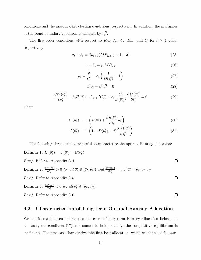
where µt, λt and φt denote the multipliers for the resource constraints, the implementability
15
conditions and the asset market clearing conditions, respectively. In addition, the multiplier
of the bond boundary condition is denoted by νBt .
The first-order conditions with respect to Kt+1, Nt, Ct, Bt+1 and θ∗t for t ≥ 1 yield,
respectively
µt − φt = βµt+1 (MPK,t+1 + 1− δ) (25)
1 + λt = µtMPN,t (26)
µt =θ
Ct
− φt
(
1
D(θ∗t )− 1
)
(27)
βtφt − βtνBt = 0 (28)
∂W (θ∗t )
∂θ∗t+ λtH(θ∗t )− λt+1J(θ
∗t ) + φt
Ct
D(θ∗t )2
∂D (θ∗t )
∂θ∗t= 0 (29)
where
H (θ∗t ) ≡
(
R(θ∗t ) +∂R(θ∗t )
∂θ∗tθ∗t
)
(30)
J (θ∗t ) ≡
(
1−D(θ∗t )− θ∗t∂D (θ∗t )
∂θ∗t
)
(31)
The following three lemma are useful to characterize the optimal Ramsey allocation:
Lemma 1. H (θ∗t ) = J (θ∗t ) = F(θ∗t )
Proof. Refer to Appendix A.4
Lemma 2.∂W (θ∗t )
∂θ∗t> 0 for all θ∗t ∈ (θL, θH) and
∂W (θ∗t )
∂θ∗t= 0 if θ∗t = θL or θH
Proof. Refer to Appendix A.5
Lemma 3.∂D(θ∗t )
∂θ∗t< 0 for all θ∗t ∈ (θL, θH)
Proof. Refer to Appendix A.6
4.2 Characterization of Long-term Optimal Ramsey Allocation
We consider and discuss three possible cases of long term Ramsey allocation below. In
all cases, the condition (17) is assumed to hold; namely, the competitive equilibrium is
inefficient. The first case characterizes the first-best allocation, which we define as follows:
16

Definition 2. In our model economy, the first-best allocation is defined as a situation where
both the aggregate efficiency and individual efficiency are achieved; namely, the MGR holds
and the borrowing constraints do not bind for all households in all states.
4.2.1 Case 1: First-best Steady State
Proposition 4. Suppose θH < ∞ and B is sufficiently large such that the debt limit con-
straint B ≤ B does not bind. Then there exists a first-best steady-state Ramsey allocation,
which features the following properties:
1. Individual efficiency is achieved —the optimal choice of θ∗t is a corner solution at θ∗t =
θH so that no households face a positive probability of binding borrowing constraints.
2. Aggregate efficiency is achieved —the MGR holds and there is no liquidity premium
(R = 1). The equilibrium interest rate equals 1/β.
3. Capital tax is zero and labor tax is positive at rate λ1+λ
< 1. The government expen-
ditures as well as bond interest payments are financed solely by revenues from labor
income tax.
Proof. See Appendix A.7
The above proposition states that if the support of θ is bounded and the debt limit
for government bond does not bind, then the Ramsey planner can pick an competitive
equilibrium that achieves both aggregate efficiency and individual efficiency — the first-best
allocation under our definition. More importantly, the Ramsey planner achieves the MGR
without the need to tax capital — the buffer stock of households, as capital taxation would
undermine individual efficiency by discouraging households’ marginal propensity to save.
Instead, the Ramsey planner provides enough incentives for households to save by picking a
sufficiently high level of interest rate on government bond such that all households are fully
self-insured with zero probability of a binding liquidity constraint.
Obviously, the first-best allocation can be archived only if the Ramsey planner is capable
of supplying enough bonds to satisfy the liquidity demand by each household across all states.
17

To shed light on this issue further, we study what happens if the government’s ability to
issue bond is limited.
4.2.2 Case 2: Steady State with a Binding Debt Limit
Now consider the case in which the constraint B ≤ B binds.
Proposition 5. There exists a steady-state Ramsey allocation with the following properties:
1. No individual efficiency — the optimal choice of θ∗t is interior and there is always a
non-zero fraction of households facing binding borrowing constraints in every period.
2. No aggregate efficiency — the modified golden rule does not hold and there is a positive
liquidity premium (R > 1). The equilibrium interest rate is less than 1/β.
3. Capital tax rate could be positive, zero, or negative, depending on the tightness of the
constraint on government debt.
Proof. See Appendix A.8
Obviously, a special sub-case is when government cannot issue bonds, B = 0. This sub-
case is analogous to the situation discussed in Proposition 2, where the equilibrium interest
rate is strictly less than the time discount rate. In such a situation, the Ramsey planner
cannot use government bond to manipulate the market interest rate and divert household
savings away from capital formation, it hence faces a trade off between achieving the MGR
by taxing capital (and thus sacrificing individual efficiency) and achieving full self-insurance
by subsidizing capital (and thus sacrificing the MGR).
In general, when the government is unable to supply enough bonds to meet the house-
holds’ demand for buffer-stock savings, either because θH is sufficiently large or the debt
limit B is sufficiently small, the pursuit of individual efficiency by the Ramsey planner will
necessarily lead to a binding constraint on government debt. In this case, there is a steady
state where neither individual efficiency nor social efficiency is achieved.
More specifically, the result of this case shows that if the individual efficiency cannot be
achieved, then the aggregate efficiency must also be sacrificed. This point can be seen clearly
18
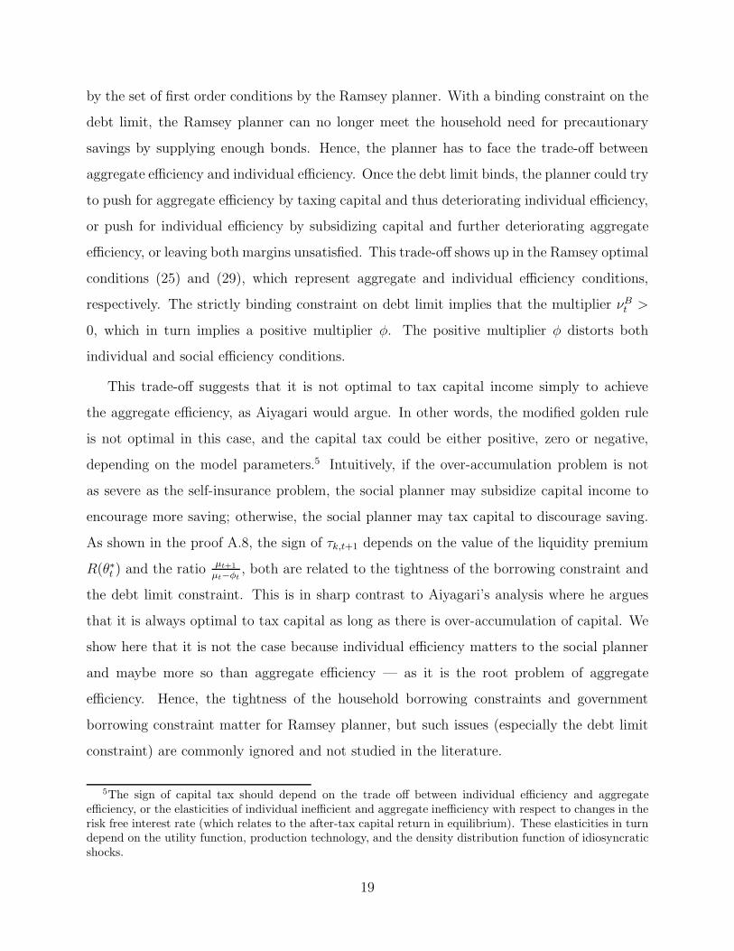
by the set of first order conditions by the Ramsey planner. With a binding constraint on the
debt limit, the Ramsey planner can no longer meet the household need for precautionary
savings by supplying enough bonds. Hence, the planner has to face the trade-off between
aggregate efficiency and individual efficiency. Once the debt limit binds, the planner could try
to push for aggregate efficiency by taxing capital and thus deteriorating individual efficiency,
or push for individual efficiency by subsidizing capital and further deteriorating aggregate
efficiency, or leaving both margins unsatisfied. This trade-off shows up in the Ramsey optimal
conditions (25) and (29), which represent aggregate and individual efficiency conditions,
respectively. The strictly binding constraint on debt limit implies that the multiplier νBt >
0, which in turn implies a positive multiplier φ. The positive multiplier φ distorts both
individual and social efficiency conditions.
This trade-off suggests that it is not optimal to tax capital income simply to achieve
the aggregate efficiency, as Aiyagari would argue. In other words, the modified golden rule
is not optimal in this case, and the capital tax could be either positive, zero or negative,
depending on the model parameters.5 Intuitively, if the over-accumulation problem is not
as severe as the self-insurance problem, the social planner may subsidize capital income to
encourage more saving; otherwise, the social planner may tax capital to discourage saving.
As shown in the proof A.8, the sign of τk,t+1 depends on the value of the liquidity premium
R(θ∗t ) and the ratio µt+1
µt−φt, both are related to the tightness of the borrowing constraint and
the debt limit constraint. This is in sharp contrast to Aiyagari’s analysis where he argues
that it is always optimal to tax capital as long as there is over-accumulation of capital. We
show here that it is not the case because individual efficiency matters to the social planner
and maybe more so than aggregate efficiency — as it is the root problem of aggregate
efficiency. Hence, the tightness of the household borrowing constraints and government
borrowing constraint matter for Ramsey planner, but such issues (especially the debt limit
constraint) are commonly ignored and not studied in the literature.
5The sign of capital tax should depend on the trade off between individual efficiency and aggregateefficiency, or the elasticities of individual inefficient and aggregate inefficiency with respect to changes in therisk free interest rate (which relates to the after-tax capital return in equilibrium). These elasticities in turndepend on the utility function, production technology, and the density distribution function of idiosyncraticshocks.
19
Aiyagari (1994, 1995) argue that the equilibrium interest rate has to be lower than 1/β.
Otherwise, individual’s asset demand goes to infinity, which cannot be a competitive equilib-
rium. But how close to 1/β the interest rate can be is never studied in the literature. In our
model, however, household’s asset demand remains finite even if the interest rate equals 1/β,
provided that the upper bound θH is finite. This property of our model makes individual
allocative efficiency feasible (achievable) since household’s marginal utility of consumption
does not follow a supermartingale process when r = 1/β, thus a finite stock of precaution-
ary savings may be sufficient for households to buffer idiosyncratic shocks without being
borrowing-constrained. As aforementioned, this finitely-valued asset demand property at
r = 1/β has to do with an important feature of our model that the expected shadow price of
consumption goods is the same across households under quasi-linear preferences. Nonethe-
less, household’s asset demand can be unbounded in our model at r = 1/β if preference
shocks are unbounded. This situation would be similar to that in the Aiyagari model.
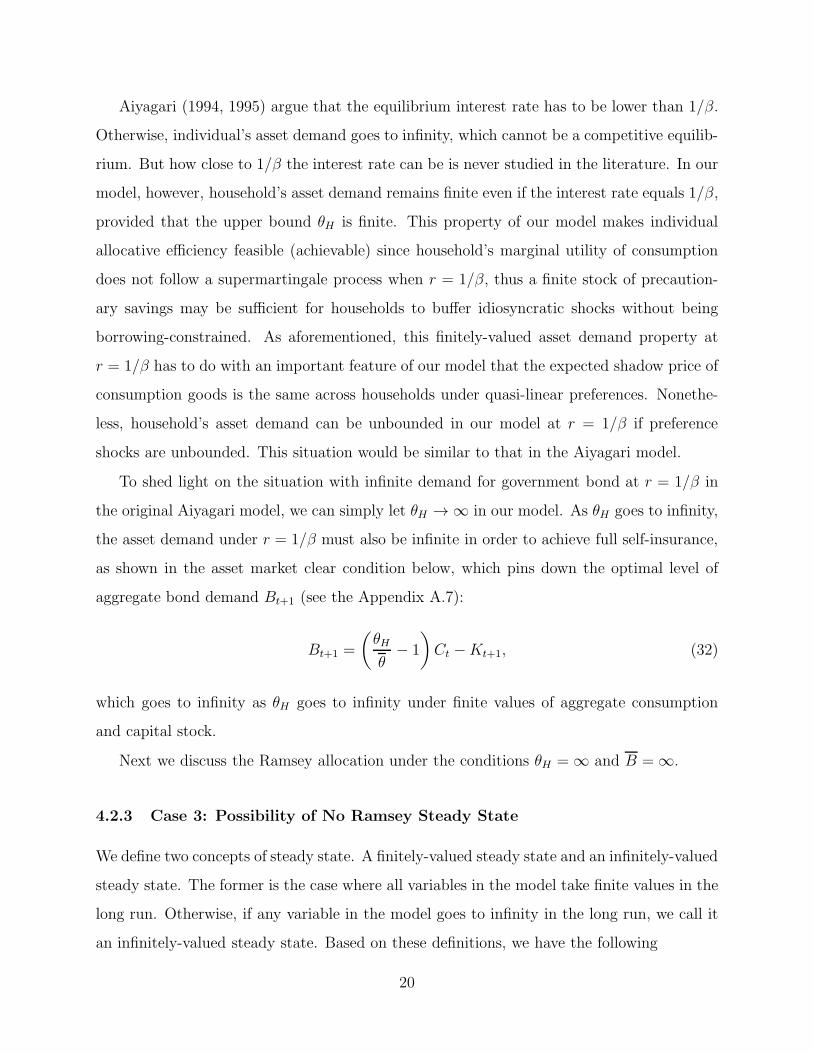
To shed light on the situation with infinite demand for government bond at r = 1/β in
the original Aiyagari model, we can simply let θH → ∞ in our model. As θH goes to infinity,
the asset demand under r = 1/β must also be infinite in order to achieve full self-insurance,
as shown in the asset market clear condition below, which pins down the optimal level of
aggregate bond demand Bt+1 (see the Appendix A.7):
Bt+1 =
(
θH
θ− 1
)
Ct −Kt+1, (32)
which goes to infinity as θH goes to infinity under finite values of aggregate consumption
and capital stock.
Next we discuss the Ramsey allocation under the conditions θH = ∞ and B = ∞.
4.2.3 Case 3: Possibility of No Ramsey Steady State
We define two concepts of steady state. A finitely-valued steady state and an infinitely-valued
steady state. The former is the case where all variables in the model take finite values in the
long run. Otherwise, if any variable in the model goes to infinity in the long run, we call it
an infinitely-valued steady state. Based on these definitions, we have the following
20

Proposition 6. There may not exist a Ramsey steady state if θH = ∞ and B = ∞.
Proof. See Appendix A.9
In the Appendix A.9, we first prove that there does not exist any finitely-valued Ramsey
steady state, and then we show that an infinitely-valued Ramsey steady state may also not
exist.
The Ramsey planner may choose a long-term allocation featuring no steady state because
of the strong motive to pursue individual efficiency, which is infeasible when θH = ∞.
Without debt limits, the Ramsey planner may attempt to issue an ever increasing amount
of government debt to archive the allocation of individual efficiency, as shown in equation
(29). Given that θH is infinite, the only path to approach the individual allocative efficiency
is through supplying an ever-increasing amount of government bond. However, an increasing
amount of bond also makes the government budget constraint harder and harder to satisfy
because of the increasing burden of interest payment. This implies an increasing value of the
multiplier on the implementability condition, λt. In addition, the increasing bond position
also makes the resource constraint tighter and tighter for the Ramsey planner over time, so
that the multiplier on resource constraint µt is also increasing over time. The everlasting
endeavor of relaxing borrowing constraints may induce the Ramsey planner to play a Ponzi
game. Also, as in the previous case, there is no clear direction on the sign of capital tax
in the long run. It all depends on the trade off between individual and aggregate allocative
efficiencies.
This possibility of no steady state provides a warning for the literature that uses numerical
methods to compute Ramsey taxation, which often assumes the existence of a steady state
and unlimited capacity to issue government debts.
5 Endogenous Government Spending
In this subsection we allow endogenous government spending in our model, as in Aiyagari
(1995). With the assumption of endogenous government spending in household utilities,
Aiyagari (1995) argues that the Ramsey planner cares only about MGR (aggregate effi-
21
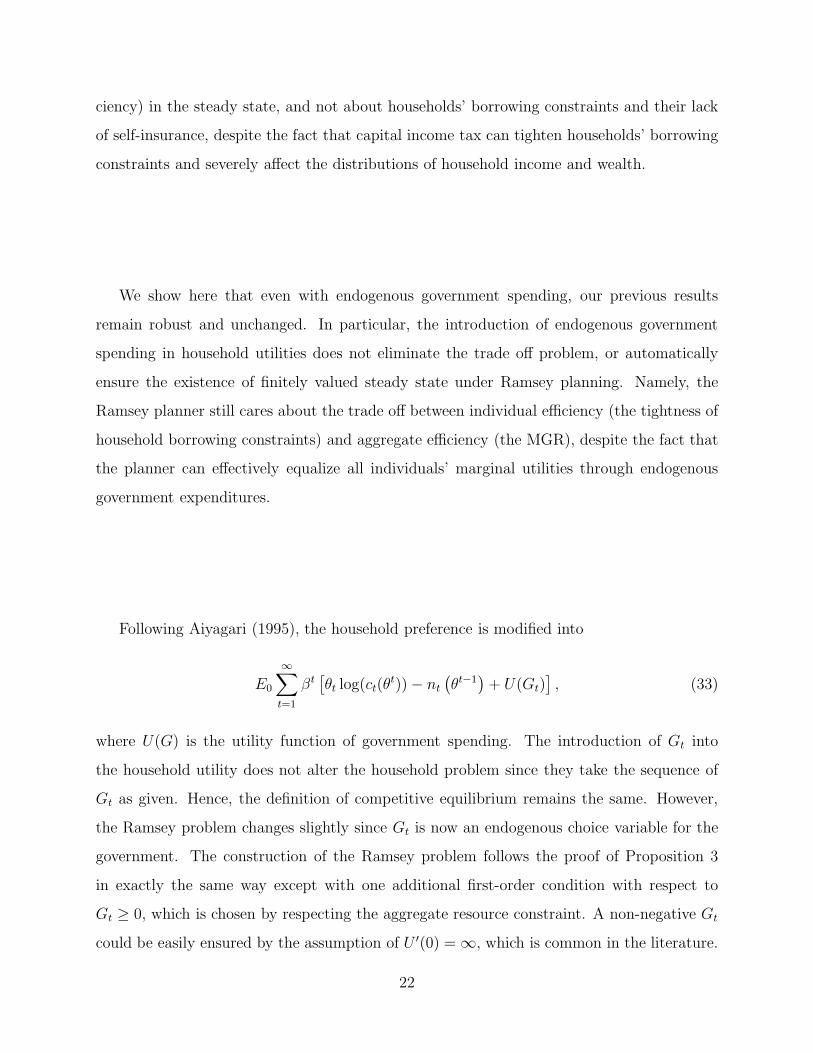
ciency) in the steady state, and not about households’ borrowing constraints and their lack
of self-insurance, despite the fact that capital income tax can tighten households’ borrowing
constraints and severely affect the distributions of household income and wealth.
We show here that even with endogenous government spending, our previous results
remain robust and unchanged. In particular, the introduction of endogenous government
spending in household utilities does not eliminate the trade off problem, or automatically
ensure the existence of finitely valued steady state under Ramsey planning. Namely, the
Ramsey planner still cares about the trade off between individual efficiency (the tightness of
household borrowing constraints) and aggregate efficiency (the MGR), despite the fact that
the planner can effectively equalize all individuals’ marginal utilities through endogenous
government expenditures.
Following Aiyagari (1995), the household preference is modified into
E0
∞∑
t=1
βt[
θt log(ct(θt))− nt
(
θt−1)
+ U(Gt)]
, (33)
where U(G) is the utility function of government spending. The introduction of Gt into
the household utility does not alter the household problem since they take the sequence of
Gt as given. Hence, the definition of competitive equilibrium remains the same. However,
the Ramsey problem changes slightly since Gt is now an endogenous choice variable for the
government. The construction of the Ramsey problem follows the proof of Proposition 3
in exactly the same way except with one additional first-order condition with respect to
Gt ≥ 0, which is chosen by respecting the aggregate resource constraint. A non-negative Gt
could be easily ensured by the assumption of U ′(0) = ∞, which is common in the literature.
22

Therefore, the Lagrangian of the Ramsey problem is modified only slightly:
L = max{θ∗t ,Nt,Ct,Kt+1,Bt+1,Gt+1}
∞∑
t=0
βt[
W (θ∗t ) + θ logCt −Nt + U(Gt)]
(34)
+βtµt (F (Kt, Nt) + (1− δ)Kt −Gt − Ct −Kt+1)
+βtλt
(
R(θ∗t )θ∗t −Nt −
θ∗t−1
β
(
1−D(θ∗t−1))
)
+βtφt
(
Kt+1 +Bt+1 −
(
1
D(θ∗t )− 1
)
Ct
)
+βtνBt (B − Bt+1)
The first order conditions with respect to Kt+1, Nt, Ct, Bt+1 and θ∗t are exactly identical
to those in equations (25), (26), (27), (28) and (29), respectively. The additional first-order
condition with respect to Gt is given by
U ′(Gt) = µt, (35)
which together with equation (25) gives exactly the same Ramsey Euler equation as in
Aiyagari (1995, eq.(20) p.1170). Suppose we follow Aiyagari by assuming that a Ramsey
steady state exists, then equation (25) becomes the MGR. Given MGR, if we also pretend
that the equilibrium interest rate in our model is below the time discount rate, we would
immediately obtain that capital tax should be positive.
However, the assumptions of a steady state and a low interest rate are not necessarily
consistent with all the first-order conditions. But these first-order conditions are ignored
in Aiyagari’s analysis. In particular, after taking all necessary first-order conditions into
account, we have shown previously that a finitely-valued steady state consistent with the
MGR exists if and only if θH is sufficiently small and the debt limit B is sufficiently large
so that the constraint Bt ≤ B does not bind. And even in this case we have shown that
the Ramsey planner achieves the MGR only by eliminating individual inefficiency instead
of by taxing capital. It is straightforward to see that such results continue to hold here by
following our analysis in Section 4 and the first-order conditions provided therein. It is also
true here that a steady state may violate the MGR if the debt limit constraint binds, and
23
that a steady state may not even exist if θH = ∞ and B = ∞. These results are in sharp
contrast to the claims of Aiyagari (1995) under the assumption of endogenous government
spending.
6 Conclusion
This paper uses a tractable model to address a long-standing problem in the optimal Ramsey
capital taxation literature. The tractability of our model enables us to solve the Ramsey
problem analytically along the entire transitional path. We show that the conventional wis-
dom on Ramsey tax policy and its underlaying intuition and rationales do not hold in our
model and may thus be misrepresented in the literature in general. We reveal the trade-off
mechanisms and conditions for the Ramsey planner to improve aggregate allocative efficiency
and individual allocative efficiency through the tools of government debt and taxes. We show
clearly in a transparent way that government debt plays an important role in determining
the optimal Ramsey outcome. The planner always intends to supply enough bond to relax
individuals’ borrowing constraints and through which to achieve the modified golden rule
by crowding out capital. Capital tax is not the vital tool to achieve aggregate allocative
efficiency despite over-accumulation of capital. Thus the optimal capital tax can be zero,
positive, or even negative, depending on the Ramsey planner’s ability to issue debt. We
prove that the modified golden rule fails to hold whenever the government encounters a debt
limit and that taxing capital is not necessarily optimal even in this case. In contrast to
the arguments of Aiyagari (1995), the planner does not levy capital tax solely to satisfy the
modified golden rule. Instead, the planner may even subsidize capital to encourage more
precautionary savings despite over-accumulation of capital. Finally, the desire to relax indi-
viduals’ borrowing constraints by the planner may lead to an increasing debt accumulation,
resulting in a dynamic path featuring no steady state. Hence, numerical approaches to solve
the Ramsey problem by assuming the existence of a finitely-valued steady state may be
incorrect.
24
References
Acikgoz, O. (2013): “Transitional Dynamics and Long-run Optimal Taxation Under In-
complete Markets,” MPRA Paper 50160, University Library of Munich, Germany.
Aiyagari, S. R. (1994): “Uninsured Idiosyncratic Risk and Aggregate Saving,” Quarterly
Journal of Economics, 109(3), 659–684.
Aiyagari, S. R. (1995): “Optimal Capital Income Taxation with Incomplete Markets,
Borrowing Constraints, and Constant Discounting,” Journal of Political Economy, 103(6),
1158–75.
Aiyagari, S. R., and E. R. McGrattan (1998): “The optimum quantity of debt,”
Journal of Monetary Economics, 42(3), 447–469.
Bewley, T. (1980): “The Optimum Quantity of Money,” in Models of Monetary
Economies, ed. by J. H. Kareken, and N. Wallace, pp. 169–210. Federal Reserve Bank
of Minneapolis, Minneapolis.
Camera, G., and Y. Chien (2014): “Understanding the Distributional Impact of Long-
Run Inflation,” Journal of Money, Credit and Banking, 46(6), 1137–1170.
Chamley, C. (2001): “Capital income taxation, wealth distribution and borrowing con-
straints,” Journal of Public Economics, 79(1), 55–69.
Conesa, J. C., S. Kitao, and D. Krueger (2009): “Taxing Capital? Not a Bad Idea
after All!,” American Economic Review, 99(1), 25–48.
Davila, J., J. H. Hong, P. Krusell, and J.-V. Rıos-Rull (2012): “Constrained Effi-
ciency in the Neoclassical Growth Model with Uninsurable Idiosyncratic Shocks,” Econo-
metrica, 80(6), 2431–2467.
Deaton, A. (1991): “Saving and Liquidity Constraints,” Econometrica, 59(5), 1221–1248.
Domeij, D., and J. Heathcote (2004): “On the Distributional Effects of Reducing Cap-
ital Taxes,” International Economic Review, 45(2), 523–554.
25
Dyrda, S., and M. Pedroni (2015): “Optimal Fiscal Policy in a Model with Uninsurable
Idiosyncratic Shocks,” Working papers, University of Toronto, Department of Economics.
Gottardi, P., A. Kajii, and T. Nakajima (2015): “Optimal Taxation and Debt
with Uninsurable Risks to Human Capital Accumulation,” American Economic Review,
105(11), 3443–3470.
Huggett, M. (1993): “The Risk-Free Rate in Heterogeneous-Agent Incomplete-Insurance
Economies,” Journal of Economic Dynamics and Control, 17(5-6), 953–969.
Kehoe, T. J., and D. K. Levine (1993): “Debt-Constrained Asset Markets,” Review of
Economic Studies, 60(4), 865–888.
Ljungqvist, L., and T. J. Sargent (2012): Recursive Macroeconomic Theory, Third
Edition, MIT Press Books. The MIT Press.
Lucas, Robert E, J. (1980): “Equilibrium in a Pure Currency Economy,” Economic
Inquiry, 18(2), 203–220.
Park, Y. (2014): “Optimal Taxation in a Limited Commitment Economy,” Review of
Economic Studies, 81(2), 884–918.
Straub, L., and I. Werning (2014): “Positive Long-Run Capital Taxation: Chamley-
Judd Revisited,” NBER Working Papers 20441, National Bureau of Economic Research,
Inc.
Wen, Y. (2009): “An analytical approach to buffer-stock saving,” Working Papers 2009-026,
Federal Reserve Bank of St. Louis.
(2015): “Money, liquidity and welfare,” European Economic Review, 76(C), 1–24.
26
A Appendix
A.1 Proof of Proposition 1
Denoting {βtλt(θt), βtµt(θ
t)} as the Lagrangian multipliers for constraints (6) and (7), re-
spectively, the first-order conditions for {ct (θt) , nt (θ
t−1) , at+1 (θt)} are given, respectively,
byθt
ct (θt)= λt
(
θt)
(36)
1 = wt
∫
λt
(
θt)
dF(θt) (37)
λt
(
θt)
= βrt+1Et
[
λt+1
(
θt+1)]
+ µt(θt), (38)
where equation (37) reflects the fact that labor supply nt(θt−1) must be chosen before the
idiosyncratic taste shocks (and hence before the value of λt(θt)) are realized. By the law of
iterated expectations and the iid assumption of idiosyncratic shocks, equation (38) can be
written as (using equation (37))
λt(θt) = β
rt+1
wt+1+ µt(θ
t), (39)
where 1wis the marginal utility of consumption in terms of labor income.
We adopt a guess-and-verify strategy to derive the decision rules. The decision rules
for an individual’s consumption and savings are characterized by a cutoff strategy, taking
as given the aggregate states (such as interest rate and real wage). Anticipating that the
optimal cutoff θ∗t is independent of individual’s history of shocks, consider two possible cases:
Case A. θt ≤ θ∗t . In this case the urge to consume is low. It is hence optimal to save so
as to prevent possible liquidity constraints in the future. So at+1(θt) ≥ 0, µt(θ
t) = 0 and the
shadow value
λt(θt) = β
rt+1
wt+1
≡ Λt,
where Λt depends only on aggregate states. Notice that λt (θt) = λt is independent of
the history of idiosyncratic shocks. Equation (36) implies that consumption is given by
ct(θt) = θtΛ
−1t . Defining xt(θ
t−1) ≡ rtat(θt−1) + wtnt(θ
t−1) as the gross income of the
27

household, the budget identity (6) then implies at+1(θt) = xt(θ
t−1)−θtΛ−1t . The requirement
at+1(θt) ≥ 0 then implies
θt ≤ Λtxt ≡ θ∗t , (40)
which defines the cutoff θ∗t .
We conjecture that the cutoff is independent of the idiosyncratic state, then the optimal
gross income xt is also independent of the idiosyncratic state. The intuition is that xt
is determined before the realization of θt and all households face the same distribution of
idiosyncratic shocks. Since the utility function is quasi-linear, the household is able to adjust
labor income to meet any target level of liquidity in hand. As a result, the distribution of
xt is degenerate. This property simplifies the model tremendously.
Case B. θt > θ∗t . In this case the urge to consume is high. It is then optimal not to save,
so at+1(θt) = 0 and µt(θ
t) > 0. By the resource constraint (6), we have ct(θt) = xt, which by
equation (40) implies ct(θt) = θ∗tΛ
−1t . Equation (36) then implies that the shadow value is
given by λt(θt) = θt
θ∗tΛt. Since θt > θ∗, equation (39) implies µt(θ
t) = Λt
[
θtθ∗t
− 1]
> 0. Notice
that the shadow value of goods (the marginal utility of income), λt(θt), is higher under case
B than under case A because of the binding borrowing constraint.
The above analyses imply that the expected shadow value of income,∫
λt(θ)dF(θ), and
hence the optimal cutoff value θ∗, is determined by equation (37) by plugging in the expres-
sions for λt (θt) under case A and B, which immediately gives equation (12). Specifically,
combining Case A and Case B, we have
λt(θt) = β
rt+1
wt+1for θ ≤ θ∗t
λt(θt) =
θtθ∗tβrt+1
wt+1for θt ≥ θ∗t ,
the aggregate Euler equation is therefore given by
1
wt
=
∫
λt(θ)dF(θ) = βrt+1
wt+1
[
∫
θ≤θ∗t
dF(θ) +
∫
θ>θ∗t
θ
θ∗dF(θ)
]
= βrt+1
wt+1R(θ∗t ),
which is equation (12). This equation reveals that the optimal cutoff depends only on
28
aggregate states and is independent of individual history.
We also immediately obtain
xt = θ∗t
(
βrt+1
wt+1
)−1
= θ∗tR(θ∗t )wt,
which leads to equation (8). By the discussion of case A and B as well as utilizing equation
(8), the decision rules of household consumption and saving can then be summarized by
equations (9) and (10), respectively. Finally, the decision rule of household labor supply,
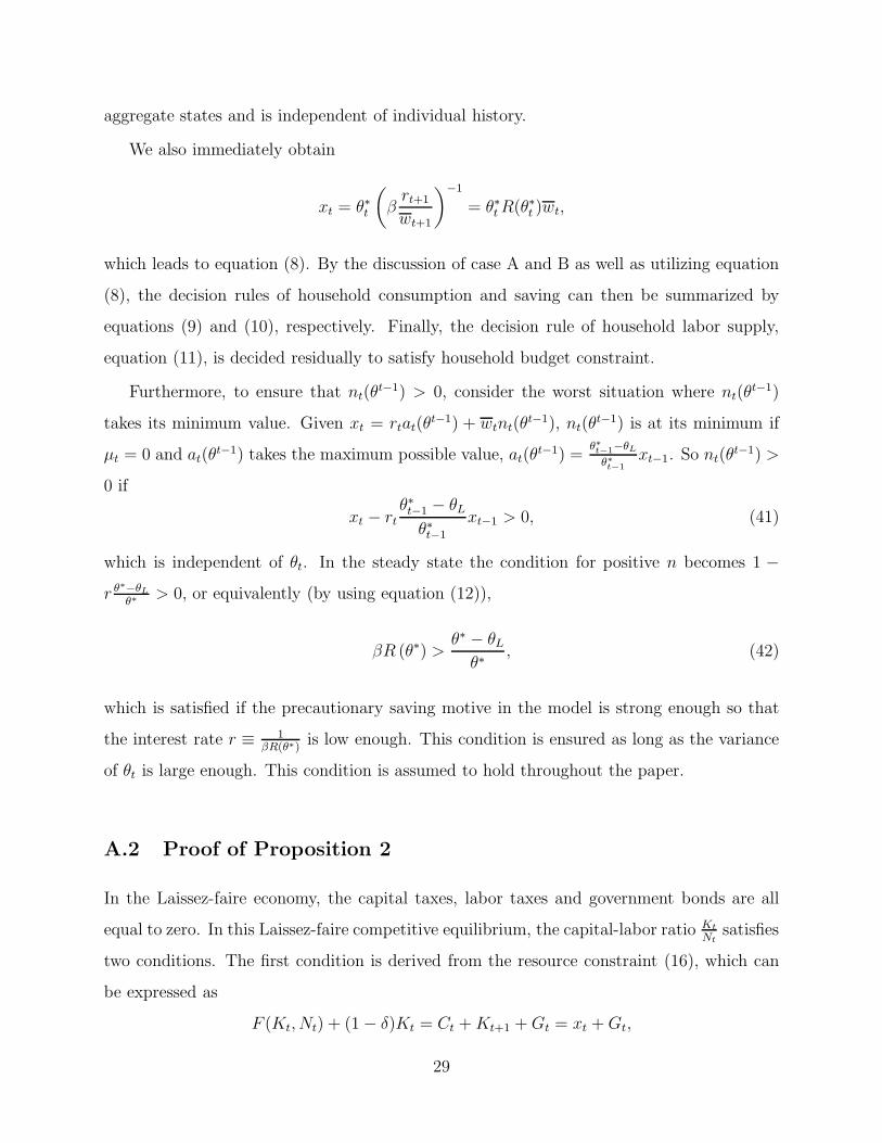
equation (11), is decided residually to satisfy household budget constraint.
Furthermore, to ensure that nt(θt−1) > 0, consider the worst situation where nt(θ
t−1)
takes its minimum value. Given xt = rtat(θt−1) + wtnt(θ
t−1), nt(θt−1) is at its minimum if
µt = 0 and at(θt−1) takes the maximum possible value, at(θ
t−1) =θ∗t−1−θL
θ∗t−1
xt−1. So nt(θt−1) >
0 if
xt − rtθ∗t−1 − θL
θ∗t−1
xt−1 > 0, (41)
which is independent of θt. In the steady state the condition for positive n becomes 1 −
r θ∗−θLθ∗
> 0, or equivalently (by using equation (12)),
βR (θ∗) >θ∗ − θL
θ∗, (42)
which is satisfied if the precautionary saving motive in the model is strong enough so that
the interest rate r ≡ 1βR(θ∗)
is low enough. This condition is ensured as long as the variance
of θt is large enough. This condition is assumed to hold throughout the paper.
A.2 Proof of Proposition 2
In the Laissez-faire economy, the capital taxes, labor taxes and government bonds are all
equal to zero. In this Laissez-faire competitive equilibrium, the capital-labor ratio Kt
Ntsatisfies
two conditions. The first condition is derived from the resource constraint (16), which can
be expressed as
F (Kt, Nt) + (1− δ)Kt = Ct +Kt+1 +Gt = xt +Gt,
29
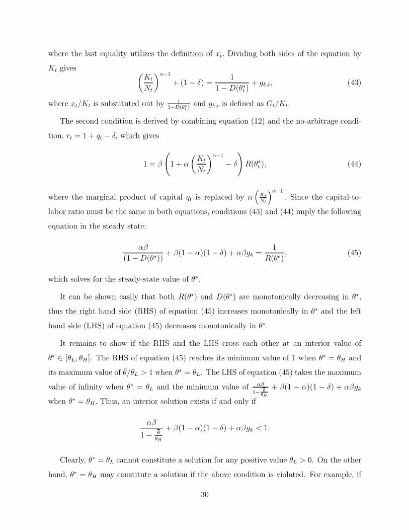
where the last equality utilizes the definition of xt. Dividing both sides of the equation by
Kt gives(
Kt
Nt
)α−1
+ (1− δ) =1
1−D(θ∗t )+ gk,t, (43)
where xt/Kt is substituted out by 11−D(θ∗t )
and gk,t is defined as Gt/Kt.
The second condition is derived by combining equation (12) and the no-arbitrage condi-
tion, rt = 1 + qt − δ, which gives
1 = β
(
1 + α
(
Kt
Nt
)α−1
− δ
)
R(θ∗t ), (44)
where the marginal product of capital qt is replaced by α(
Kt
Nt
)α−1
. Since the capital-to-
labor ratio must be the same in both equations, conditions (43) and (44) imply the following
equation in the steady state:
αβ
(1−D(θ∗))+ β(1− α)(1− δ) + αβgk =
1
R(θ∗), (45)
which solves for the steady-state value of θ∗.
It can be shown easily that both R(θ∗) and D(θ∗) are monotonically decreasing in θ∗,
thus the right hand side (RHS) of equation (45) increases monotonically in θ∗ and the left
hand side (LHS) of equation (45) decreases monotonically in θ∗.
It remains to show if the RHS and the LHS cross each other at an interior value of
θ∗ ∈ [θL, θH ]. The RHS of equation (45) reaches its minimum value of 1 when θ∗ = θH and
its maximum value of θ/θL > 1 when θ∗ = θL. The LHS of equation (45) takes the maximum
value of infinity when θ∗ = θL and the minimum value of αβ
1− θθH
+ β(1 − α)(1 − δ) + αβgk
when θ∗ = θH . Thus, an interior solution exists if and only if
αβ
1− θθH
+ β(1− α)(1− δ) + αβgk < 1.
Clearly, θ∗ = θL cannot constitute a solution for any positive value θL > 0. On the other
hand, θ∗ = θH may constitute a solution if the above condition is violated. For example, if
30

θH is small and close enough to the mean θ, then the above condition does not hold since
its LHS approaches infinity when θH → θ. On the other hand, if θH → ∞, as in the case of
Pareto distribution, then 1− θθH
→ 1. In this case, the LHS is less than 1 if gk = 0 or small
enough.
Therefore, an interior solution for θ∗ exists if the upper bound of the idiosyncratic shock
is large enough. Otherwise we have the corner solution θ∗ = θH . Finally, if θ∗ is an interior
solution, then R(θ∗) > 1 and r < 1/β by equation (12).
A.3 Proof of Proposition 3
A.3.1 The ”only if” Part
Assume that we have the allocation {θ∗t , Ct, Nt, Kt+1, Bt+1}. With this allocation, we can
directly construct the prices, taxes and individual allocations in the competitive equilibrium
in the following 7 steps:
1. wt and qt are set by (1) and (2), which are wt = MPN,t and qt = MPK,t, respectively.
2. Given Ct and θ∗t , the total liquidity in hand can be set by equation (18), xt =Ct
D(θ∗t ).
3. The individual consumption and asset holdings, ct(θt) and at+1(θt), are pinned down
by equation (9) and (10).
4. τn,t is determined by equation (8), which implies τn,t = 1− xt
R(θ∗t )θ∗
tMPN,t. Hence, wt can
be expressed as:
wt =xt
R(θ∗t )θ∗t
=Ct
D(θ∗t )R(θ∗t )θ∗t
.
Given wt, the interest rate rt+1 can be backed out by the Euler equation (12):
rt+1 =wt+1
wt
1
βR(θ∗t )=
D(θ∗t )R(θ∗t )θ∗t
D(θ∗t+1)R(θ∗t+1)θ∗t+1
Ct+1
Ct
1
βR(θ∗t )=
D(θ∗t )θ∗t
D(θ∗t+1)R(θ∗t+1)θ∗t+1
Ct+1
βCt
.
Given the expression of rt+1, the capital tax τk,t+1 is chosen to satisfy the no-arbitrage
condition: rt+1 = 1 + (1− τk,t+1)MPK,t+1 − δ.
31

5. Finally, set nt(θt−1) to satisfy equation (11), which implied by the individual household
budget constraint.
6. Define At+1 as the aggregate asset holding in period t. Integrating (10) gives
At+1 ≡
∫
at+1(θt)dF (θt) =
∫
max
{
θ∗t − θtθ∗t
, 0
}
xtdF (θt) =
(
1
D(θ∗t )− 1
)
Ct,
where the last equality utilizes equation (18). The above equation together with the
condition defined in equation (20) gives the competitive equilibrium asset market clear-
ing condition (14).
7. The implementability condition suggests that
R(θ∗t )θ∗t ≥ Nt +
θ∗t−1
β
(
1−D(θ∗t−1))
.
Multiplying both side of the above equation with Ct
D(θ∗t )R(θ∗t )θ∗
tleads to
Ct
D(θ∗t )≥
Ct
D(θ∗t )R(θ∗t )θ∗t
Nt +θ∗t−1
D(θ∗t )R(θ∗t )θ∗t
1
β
(
1−D(θ∗t−1))
Ct.
Using the relationship constructed in steps 2, 4 and 6 for xt, Ct, At+1, wt and rt into
the above equation gives
Ct + At+1 ≥ wtNt + rtAt,
which together with the resource constraint and asset market clearing condition enforce
the government budget constraint.
Step 1 ensures that the representative firm’s problem is solved. Steps 2 to 5 guarantee
the individual household problem is solved. Steps 6 and 7 ensure the asset market clearing
condition and government budget constraint are satisfied, respectively. The labor market
clearing condition is satisfied by the Walras law.
32
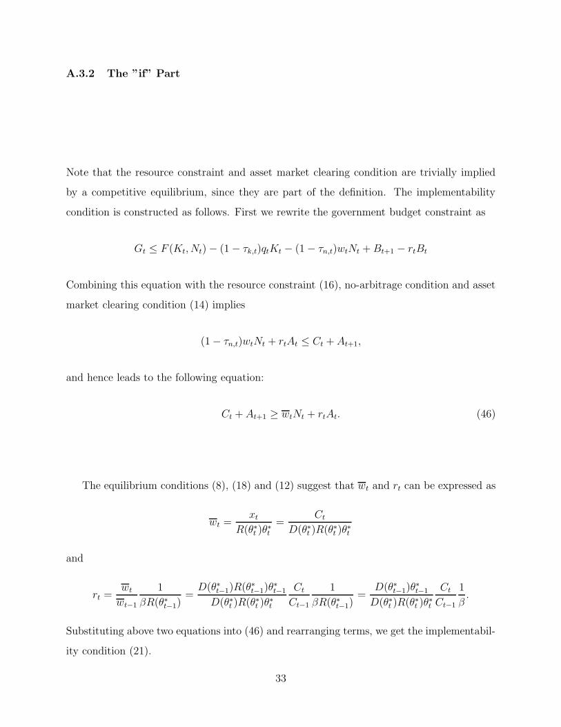
A.3.2 The ”if” Part
Note that the resource constraint and asset market clearing condition are trivially implied
by a competitive equilibrium, since they are part of the definition. The implementability
condition is constructed as follows. First we rewrite the government budget constraint as
Gt ≤ F (Kt, Nt)− (1− τk,t)qtKt − (1− τn,t)wtNt +Bt+1 − rtBt
Combining this equation with the resource constraint (16), no-arbitrage condition and asset
market clearing condition (14) implies
(1− τn,t)wtNt + rtAt ≤ Ct + At+1,
and hence leads to the following equation:
Ct + At+1 ≥ wtNt + rtAt. (46)
The equilibrium conditions (8), (18) and (12) suggest that wt and rt can be expressed as
wt =xt
R(θ∗t )θ∗t
=Ct
D(θ∗t )R(θ∗t )θ∗t
and
rt =wt
wt−1
1
βR(θ∗t−1)=
D(θ∗t−1)R(θ∗t−1)θ∗t−1
D(θ∗t )R(θ∗t )θ∗t
Ct
Ct−1
1
βR(θ∗t−1)=
D(θ∗t−1)θ∗t−1
D(θ∗t )R(θ∗t )θ∗t
Ct
Ct−1
1
β.
Substituting above two equations into (46) and rearranging terms, we get the implementabil-
ity condition (21).
33

A.4 Proof of lemma 1
H (θ∗t ) ≡
(
1−D(θ∗t )− θ∗t∂D (θ∗t )
∂θ∗t
)
= 1−
[
∫
θ≤θ∗t
θ
θ∗tdF(θ) +
∫
θ>θ∗t
dF(θ)
]
+
∫
θ≤θ∗t
θ
θ∗tdF(θ)
= 1−
∫
θ>θ∗t
dF(θ) = F(θ∗t )
J (θ∗t ) ≡
(
R(θ∗t ) +∂R(θ∗t )
∂θ∗tθ∗t
)
=
∫
θ≤θ∗t
dF(θ) +
∫
θ>θ∗t
θ
θ∗tdF(θ)−
∫
θ>θ∗t
θ
θ∗tdF(θ)
=
∫
θ≤θ∗t
dF(θ) = F(θ∗t ).
A.5 Proof of lemma 2
We first show that∂W (θ∗t )
∂θ∗t= 0 if θ∗t = θL or θH :
∂W (θ∗t )
∂θ∗t= −
∂D (θ∗t )
∂θ∗t
θ
D (θ∗t )−
∫
θ≤θ∗t
θ
θ∗tdF(θ) =
[
θ
D (θ∗t ) θ∗t
− 1
]∫
θ≤θ∗t
θ
θ∗tdF(θ)
=
[
1− θθ
θHθH
]
θθH
= 0 if θ∗t = θH[
1− θθL
]
0 = 0 if θ∗t = θL
Next, we show that∂W (θ∗t )
∂θ∗t> 0 for any θ∗t ∈ (θL, θH). Note that
D (θ∗t ) θ∗t =
∫
θ≤θ∗t
θdF(θ) + θ∗t
∫
θ>θ∗t
dF(θ) = θ −
∫
θ>θ∗t
(θ − θ∗t )dF(θ) < θ
→θ
D (θ∗t ) θ∗t
> 1
Hence,∂W (θ∗t )
∂θ∗t=
[
θ
D (θ∗t ) θ∗t
− 1
]∫
θ≤θ∗t
θ
θ∗tdF(θ) > 0
34
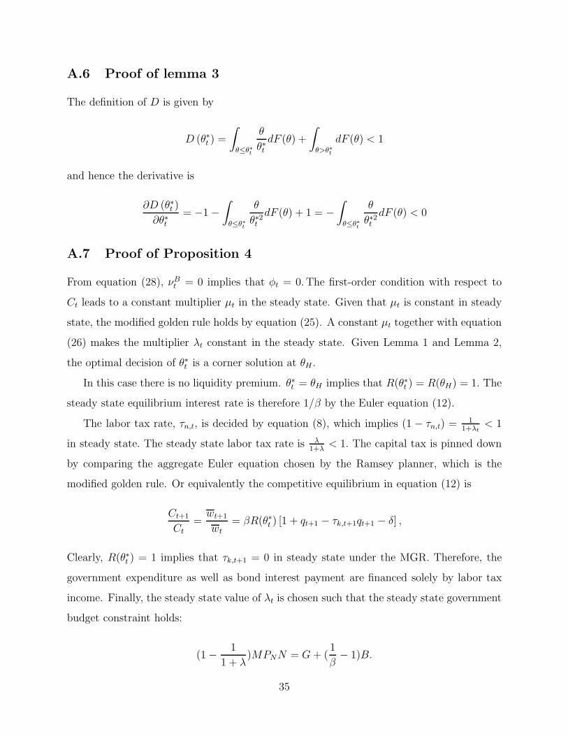
A.6 Proof of lemma 3
The definition of D is given by
D (θ∗t ) =
∫
θ≤θ∗t
θ
θ∗tdF (θ) +
∫
θ>θ∗t
dF (θ) < 1
and hence the derivative is
∂D (θ∗t )
∂θ∗t= −1−
∫
θ≤θ∗t
θ
θ∗2tdF (θ) + 1 = −
∫
θ≤θ∗t
θ
θ∗2tdF (θ) < 0
A.7 Proof of Proposition 4
From equation (28), νBt = 0 implies that φt = 0.The first-order condition with respect to
Ct leads to a constant multiplier µt in the steady state. Given that µt is constant in steady
state, the modified golden rule holds by equation (25). A constant µt together with equation
(26) makes the multiplier λt constant in the steady state. Given Lemma 1 and Lemma 2,
the optimal decision of θ∗t is a corner solution at θH .
In this case there is no liquidity premium. θ∗t = θH implies that R(θ∗t ) = R(θH) = 1. The
steady state equilibrium interest rate is therefore 1/β by the Euler equation (12).
The labor tax rate, τn,t, is decided by equation (8), which implies (1 − τn,t) =1
1+λt< 1
in steady state. The steady state labor tax rate is λ1+λ
< 1. The capital tax is pinned down
by comparing the aggregate Euler equation chosen by the Ramsey planner, which is the
modified golden rule. Or equivalently the competitive equilibrium in equation (12) is
Ct+1
Ct
=wt+1
wt
= βR(θ∗t ) [1 + qt+1 − τk,t+1qt+1 − δ] ,
Clearly, R(θ∗t ) = 1 implies that τk,t+1 = 0 in steady state under the MGR. Therefore, the
government expenditure as well as bond interest payment are financed solely by labor tax
income. Finally, the steady state value of λt is chosen such that the steady state government
budget constraint holds:
(1−1
1 + λ)MPNN = G+ (
1
β− 1)B.
35
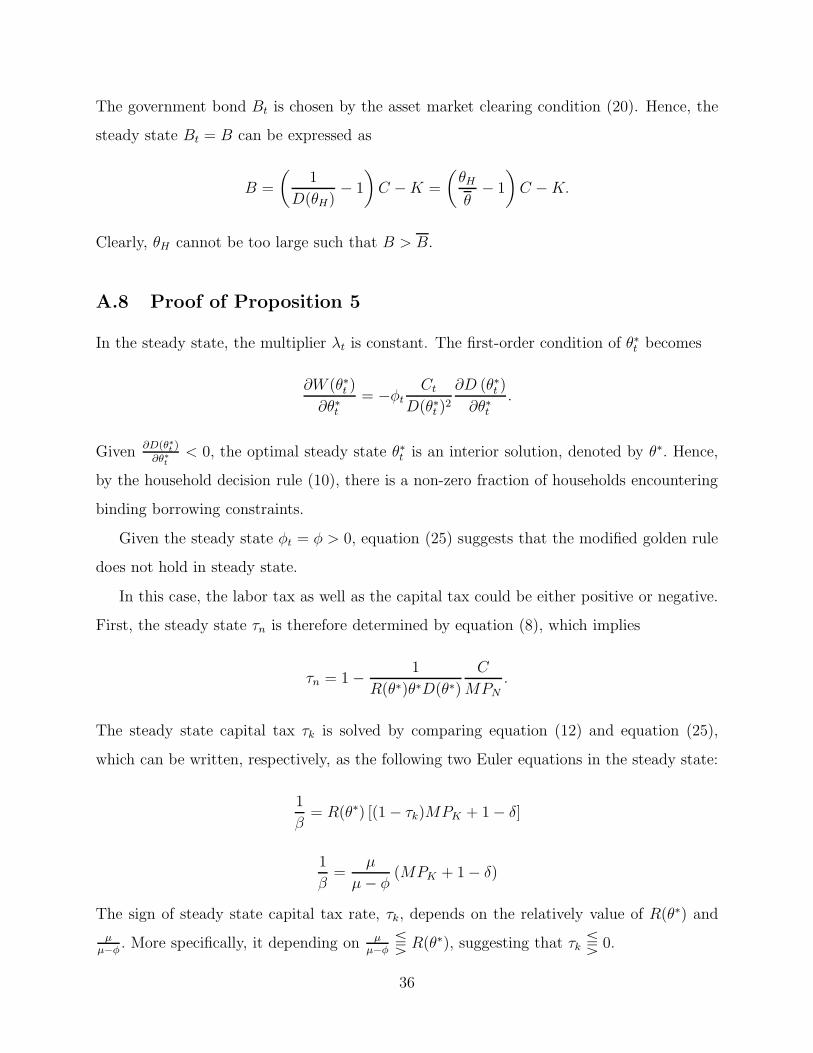
The government bond Bt is chosen by the asset market clearing condition (20). Hence, the
steady state Bt = B can be expressed as
B =
(
1
D(θH)− 1
)
C −K =
(
θH
θ− 1
)
C −K.
Clearly, θH cannot be too large such that B > B.
A.8 Proof of Proposition 5
In the steady state, the multiplier λt is constant. The first-order condition of θ∗t becomes
∂W (θ∗t )
∂θ∗t= −φt
Ct
D(θ∗t )2
∂D (θ∗t )
∂θ∗t.
Given∂D(θ∗t )
∂θ∗t< 0, the optimal steady state θ∗t is an interior solution, denoted by θ∗. Hence,
by the household decision rule (10), there is a non-zero fraction of households encountering
binding borrowing constraints.
Given the steady state φt = φ > 0, equation (25) suggests that the modified golden rule
does not hold in steady state.
In this case, the labor tax as well as the capital tax could be either positive or negative.
First, the steady state τn is therefore determined by equation (8), which implies
τn = 1−1
R(θ∗)θ∗D(θ∗)
C
MPN
.
The steady state capital tax τk is solved by comparing equation (12) and equation (25),
which can be written, respectively, as the following two Euler equations in the steady state:
1
β= R(θ∗) [(1− τk)MPK + 1− δ]
1
β=
µ
µ− φ(MPK + 1− δ)
The sign of steady state capital tax rate, τk, depends on the relatively value of R(θ∗) and
µ
µ−φ. More specifically, it depending on µ
µ−φS R(θ∗), suggesting that τk S 0.
36
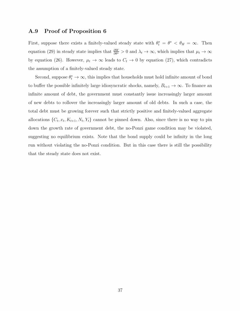
A.9 Proof of Proposition 6
First, suppose there exists a finitely-valued steady state with θ∗t = θ∗ < θH = ∞. Then
equation (29) in steady state implies that ∂W∂θ∗
> 0 and λt → ∞, which implies that µt → ∞
by equation (26). However, µt → ∞ leads to Ct → 0 by equation (27), which contradicts
the assumption of a finitely-valued steady state.
Second, suppose θ∗t → ∞, this implies that households must hold infinite amount of bond
to buffer the possible infinitely large idiosyncratic shocks, namely, Bt+1 → ∞. To finance an
infinite amount of debt, the government must constantly issue increasingly larger amount
of new debts to rollover the increasingly larger amount of old debts. In such a case, the
total debt must be growing forever such that strictly positive and finitely-valued aggregate
allocations {Ct, xt, Kt+1, Nt, Yt} cannot be pinned down. Also, since there is no way to pin
down the growth rate of government debt, the no-Ponzi game condition may be violated,
suggesting no equilibrium exists. Note that the bond supply could be infinity in the long
run without violating the no-Ponzi condition. But in this case there is still the possibility
that the steady state does not exist.
37