Optimal Process Operation for the Production of Linear ... Process Operation for the Production of Linear Polyethylene Resins with Tailored Molecular Weight Distribution ... of a living

Optimal Process Operation for the Productionof Linear Polyethylene Resins with Tailored

Molecular Weight DistributionK. V. Pontes

Industrial Engineering Program (PEI)—Universidade Federal da Bahia—R. Aristides Novis No 2,Federacao, Salvador-BA, Brazil

AVT—Process Systems Engineering, RWTH Aachen University, Turmstr. 46, 52064 Aachen, Germany

M. EmbirucuIndustrial Engineering Program (PEI)—Universidade Federal da Bahia—R. Aristides Novis No 2,

Federacao, Salvador-BA, Brazil

R. Maciel

Laboratory of Optimization, Design and Advanced Control (Lopca)—Campinas State University—CidadeUniversitaria Zeferino Vaz, Caixa Postal 1170, Campinas-SP, Brazil

A. HartwichAVT—Process Systems Engineering, RWTH Aachen University, Turmstr. 46, 52064 Aachen, Germany

German Research School for Simulation Sciences GmbH, 52064 Aachen, Germany

W. MarquardtAVT—Process Systems Engineering, RWTH Aachen University, Turmstr. 46, 52064 Aachen, Germany

DOI 10.1002/aic.12438Published online November 2, 2010 in Wiley Online Library (wileyonlinelibrary.com).

An optimization model is presented to determine optimal operating policies for tailoringhigh density polyethylene in a continuous polymerization process. Shaping the whole molec-ular weight distribution (MWD) by adopting an appropriate choice of operating conditionsis of great interest when designing new polymers or when improving quality. The continuoustubular and stirred tank reactors are modeled in steady state by a set of differential-alge-braic equations with the spatial coordinate as independent variable. A novel formulation ofthe optimization problem is introduced. It comprises a multi-stage optimization model withdifferential-algebraic equality constraints along the process path and inequality end-pointconstraints on product quality. The resulting optimal control problem is solved at high com-putational efficiency by means of a shooting method. The results show the efficiency of theproposed approach and the benefit of predicting and controlling the complete MWD as wellas the interplay between operating conditions and polymer properties. VVC 2010 American Insti-

tute of Chemical Engineers AIChE J, 57: 2149–2163, 2011

Keywords: mathematical modeling, multi-stage optimization, polymerization, reactionengineering, polyethylene, molecular weight distribution

Correspondence concerning this article should be addressed to K. V. Pontes [email protected].

VVC 2010 American Institute of Chemical Engineers

AIChE Journal 2149August 2011 Vol. 57, No. 8

Introduction

Polymer materials are present in everyday life, in seg-ments such as packing, transport, and construction. Theirend-use properties depend heavily on the operating condi-tions under which the polymer is synthesized. In industrialpractice, polymerization processes are usually operatedaccording to a predetermined recipe, which reflects availablechemical knowledge and the practical experience of the pro-cess operators. Often, the processes are operated under sub-optimal conditions due to the lack of a systematic methodfor determining the best operating policies. Today, processmodels as well as optimization tools are available and theyprovide the foundation for a systematic process and productquality improvement. As a result, there is considerable inter-est within the polymer industry to develop optimal operatingpolicies that will result in the production of polymers withdesired molecular properties.

According to Kiparissides,1 there are two classes of opti-mization problems for polymerization reactors: steady-stateoptimization, which deals with the selection of the best (op-timum) time invariant controls such that the molecular prop-erties attain certain desired values; and dynamic optimization(or optimal control), which refers to the determination ofoptimal control trajectories to move a polymer reactor fromits initial to a desired final state. The former is usuallyrelated to the steady-state operation of continuous polymerreactors while the latter is concerned with the dynamic oper-ation of batch and semibatch reactors as well as with start-up, shut-down, and grade transition policies for continuouspolymerization processes. The focus of the present article isthe optimal steady-state operation of a complex reactor con-figuration comprising a series of continuous tubular andstirred tank reactors to meet a specified polymer at the low-est production cost.

Polymer quality is usually specified in terms of end useproperties such as stiffness, melting temperature, and crystalli-zation temperature. Some attempts have been made to correlatesuch polymer end-use properties with lumped properties whichcan easily be measured in a polymer production plant. A typi-cal example is given by the melt index (MI).2,3 However,rheological and processing properties might differ significantlyif the molecular weight distribution (MWD) is skewed andshows high concentrations of high or low molecular weightfractions. In particular, Ariawan et al.4 show that the rheologi-cal properties of the polymer are affected by the completeMWD. They conclude that the extensional and elastic proper-ties are very much dependent on the distribution tail, referringto molecules with large molecular weight. Consequently, sev-eral authors developed correlations between polymer propertiesand the whole MWD. For example, Hinchliffe et al.5 proposea methodology to correlate the MI, the shear thinning ratio andthe dart impact with selected bins of the MWD. Furthermore,Nele et al.6 successfully predict the MI from the entire MWDusing convolution of the MWD and a kernel function. Morerecently, Zahedi et al.7 have used spline functions to correlateflow properties of the polymer melt with the entire MWD.Motivated by these findings, the full MWD is used in thiswork as the target quality property to be met by optimal opera-tion of the polymer production plant in steady state.

There have been many attempts to determine optimaloperating conditions of polymerization processes to produce

polymers with target average molecular weight and polydis-persity. Most of the research considered the polymerizationof methyl methacrylate (MMA) in batch reactors.8–12 How-ever, the first moments of the MWD and average propertiesare in many cases insufficient to describe polymer end-useproperties satisfactorily.4 Despite the importance of predict-ing the full MWD, as discussed previously, only few papersreport on determining optimal operating policies for polymerproduction with a target MWD. Crowley and Choi13 obtainoptimal temperature trajectories to control the MWD ofMMA produced in a batch reactor, using the method of finitemolecular weight moments for capturing MWD.14 In anothercontribution,15 the same authors determine optimal tempera-ture and initiator concentration policies to target the tensilestrength of the polystyrene produced in a batch suspensionreactor. Sayer et al.16 compute the optimal monomer andchain transfer feed profiles for MMA batch copolymerizationto produce a polymer with a specified copolymer composi-tion and MWD. Kiparissides et al.17 propose a temperaturecontrol scheme for free radical polymerization of MMA in abatch reactor. An optimization step ensures the production ofa polymer with target properties which include not only theaverage molecular weights but also the complete MWD.More recently, Kiparissides and coworkers18 use an optimi-zation model to determine the optimal temperature profilethat produces the target MWD of MMA in minimum batchtime. Vicente et al.19 target MWD, copolymer compositionand final monomer concentration in a semibatch emulsionpolymerization of MMA/n-butylacrylate and compare theoptimization results with experiments in a pilot plant. Whileall the works discussed so far report on (semi)batch poly-merization processes, Asteasuain et al.20 consider optimalsteady-state operation of a living polymerization of styrenein a tubular reactor with a targeted MWD. In a second publi-cation,21 these authors also explore the optimization modelto determine operating conditions resulting in a multimodalMWD.

Brandolin and coworkers have addressed the computationof optimal operating policies to achieve target product prop-erties in continuous polyethylene production. This groupstudied a continuous high pressure tubular reactor for theproduction of low density polyethylene (LDPE). Brandolinet al.22 derive optimal steady-state operating points (tempera-ture and initiator concentration) to attain a specific numberaverage molecular weight, polydispersity and weight averagebranch point number in the effluent product. Asteasuainet al.23 studied start-up and shutdown strategies to maximizeoutlet conversion, while satisfying the desired number aver-age molecular weight and transition time. Cervantes et al.24

have extended the dynamic reactor model to the entire plantto study optimal grade transitions for LDPE production. Thisoptimization criterion tries to minimize copolymer content inthe recycle stream as well as transition time. In thesearticles, no attempt has been made to tailor the completeMWD. In their latest work, however, Asteasuain and Bran-dolin25 focus on the optimization of an LDPE tubular reactorto maximize conversion while targeting the entire MWDthrough constraints using a steady-state model. They predictbimodal MWD when feeding monomer and chaintransfer agent at a fixed lateral injection point of the multi-stage tubular reactor with counter-currently cooling. The

2150 DOI 10.1002/aic Published on behalf of the AIChE August 2011 Vol. 57, No. 8 AIChE Journal

optimization problem has been solved in gPROMS after aspatial discretization of the differential-algebraic model tohandle the multi-point boundary conditions. More recentlyZavala and Biegler26 optimize the operation of a multi-zonetubular reactor for the production of LDPE with target melt-index and density for a sequence of decaying heat transfercoefficients. They also employ a spatially discretized formu-lation of the steady-state reactor model to obtain a large-scale nonlinear programming problem. These authors do notattempt to tailor the complete MWD of the resin.

Kiparissides’ group also studied the continuous productionof LDPE in tubular reactor for optimization and control pur-poses.27,28 The gas phase and slurry ethylene continuous pol-ymerizations were also object of studies approaching theoptimal control of grade transitions.29–32 Despite the signifi-cant amount of work on optimization of polyethylene reac-tor, to the authors’ knowledge, optimal operating policies fora continuous solution polymerization in a complex reactorconfiguration consisting of tubular and stirred tank reactorshas not yet been treated adequately in literature.

Our previous work33 has suggested a new formulation ofan optimization problem to find optimal steady-state operat-ing conditions of a continuous multi-reactor polymerizationprocess that produces a tailored polymer with a targeted MIand stress exponent (SE). In contrast to the work of otherresearch groups reviewed above, we have considered ethyl-ene polymerization in solution using a Ziegler-Natta catalystin a complex configuration of continuous stirred tank(CSTR) and plug flow reactors (PFR). The optimizationproblem formulation relies on a steady-state multi-stagemodel with the spatial coordinate as independent variablewhich—together with product quality specifications—consti-tute the constraints of an optimization problem with eco-nomic objective. The multi-stage optimal control problemreveals discontinuities with respect to the spatial coordinatedue to different types of reactors and lateral feed injectionspoints which are themselves decisions in the optimization.

This article presents an extension of our previous work fo-cusing on the production of tailored linear polyethylene, thequality of which is not only specified through lumped qualityproperties such as MI and SE but through the completeMWD. This detailed treatment of the quality specification isof great industrial importance, because of the complex trade-off between polymer properties—ultimately determined by

the MWD—and the economics of production. The polymer-ization model is complex not only due to its multi-stage andspatially distributed character but also due to the MWD usedto predict polymer quality. The original contribution of thisarticle is the efficient and accurate solution of this complexoptimization problem using a multi-stage optimal controlproblem formulation in the spatial coordinate and singleshooting rather than spatial discretization for its solution.The novel numerical approach proposed here overcomessome problems reported in previous literature, even for prob-lems of lower complexity. Furthermore, we show that poly-ethylene products with very different MWD and averagepolymer properties can be produced economically in thesame plant under different process configurations and at dif-ferent operating points. Therefore, the second original contri-bution of the article constitutes of a systematic methodologyto support product design engineers and plant operators todevelop and produce new resins or existing resins ofimproved quality, which is specified by the complete MWD.

The article is structured as follows. First, the polymeriza-tion process is described. Then, the mathematical models ofthe process and the polymer properties as well as the methodfor computing the MWD are presented. In the next section,the optimization problem is formulated and the solutionmethod is discussed and compared with previously suggestedmethods. Then, the results of several optimization runs arediscussed to illustrate the applicability, potential and effi-ciency of the proposed modelling and solution procedure.Finally, the article is concluded.

Process Description and Mathematical Model

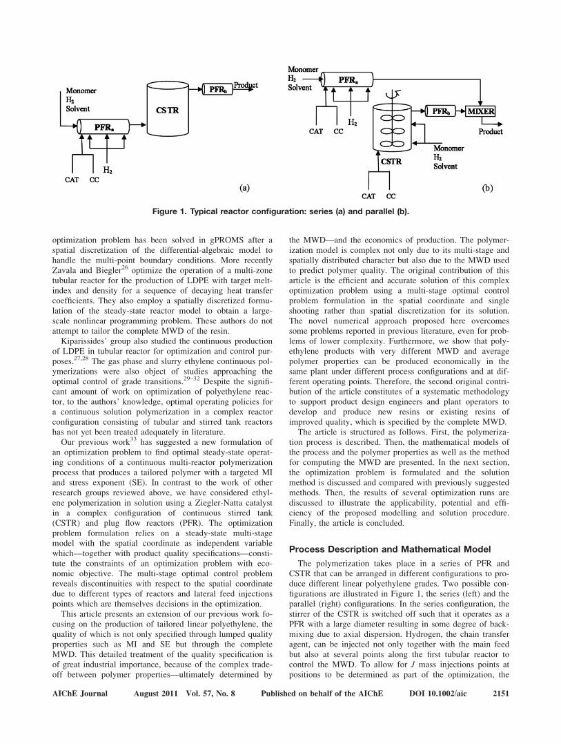
The polymerization takes place in a series of PFR andCSTR that can be arranged in different configurations to pro-duce different linear polyethylene grades. Two possible con-figurations are illustrated in Figure 1, the series (left) and theparallel (right) configurations. In the series configuration, thestirrer of the CSTR is switched off such that it operates as aPFR with a large diameter resulting in some degree of back-mixing due to axial dispersion. Hydrogen, the chain transferagent, can be injected not only together with the main feedbut also at several points along the first tubular reactor tocontrol the MWD. To allow for J mass injections points atpositions to be determined as part of the optimization, the

Figure 1. Typical reactor configuration: series (a) and parallel (b).

AIChE Journal August 2011 Vol. 57, No. 8 Published on behalf of the AIChE DOI 10.1002/aic 2151

first PFR is divided into J segments with PFR characteristics,where the starting point of compartment j is located at thelateral mass injection points. When operating the parallelconfiguration, the main feed to the CSTR can be split so thatpart of it feeds the top of the reactor in addition to the feedat the bottom.

A detailed description of the process and the mathematicalmodel is beyond the scope of this article. The appendixbriefly summarizes the kinetic mechanism, the model equa-tions and the polymer property models. For further detailson model development, we refer to Pontes et al.33 andEmbirucu et al.34–39 Model parameters, including kinetic andphysical properties constants, have been validated with ex-perimental data from an industrial polymerization process intheir work. MI and SE are used to infer the average molecu-lar weight and the polydispersity, respectively.

In our previous work33 on optimal operating policies, onlyaverage properties of the MWD have been considered,requiring only the prediction of the first three moments todescribe product quality. In contrast, the present studyfocuses on targeting the complete MWD to enable a moredetailed specification of the target polymer quality. There-fore, equations for the dead polymer concentration are alsorequired. The mass balances for the dead polymer in theCSTR and PFR are given by34,40

dUp;j

dzj¼ Up;j

qj� dqjdzj

þ rUp� A � qj

Wj;

zj 2 ð0; lj�; j ¼ 1;…; J þ 1; p ¼ 2;…;1; ð1ÞWr�1 � Up;r�1

qr�1

þ FZr � Up;r

qFZrþ Brþ1 � Up;rþ1

qrþ1

� Br þWrð Þ � Up;r

qrþ Vr � rUp

¼ 0; r ¼ 1;…;R: ð2Þ

z is the axial coordinate, lj is the length of segment j, Wj, Bj, andFZj are mass flow rates (kg/s), Up is the concentration of deadpolymer with length p (kmol/m3), rUp

is the reaction rate of deadpolymer with p monomer units (kmol/s �m3), A is the cross-sectional area (m2), q is the density of the mixture (kg/m3), Vr isthe volume of an ideal CSTR segment (m3) and J and R are thenumber of PFR and CSTR segments, respectively. The reactionrate of the dead polymer is given by40

rUp¼ P1 � fcp

kp �M þ 1

8>>:

9>>;

1�p

�fcp; p ¼ 2;…;1; (3)

fcp ¼ kfm þ ktmð Þ �M þ kfh � Hofh2 þ kth � Hoth

2

þkfcc � CCofcc þ ktcc � CCotcc þ kf þ kt; ð4Þwhere Pp is the concentration of live polymer with length p.M, H2, and CC are the monomer, hydrogen, and co-catalystconcentrations, k is the reaction rate, the subscripts f and t referto transfer and termination reactions, the indices m, h, and CCrefer to monomer, hydrogen, and co-catalyst and the exponentsofh, oth, ofcc, and otcc denote the order of transfer andtermination reactions with hydrogen and co-catalyst.

Since it is impossible to directly solve an infinite numberof mass balance equations for the dead polymer (Eqs. 1 and2), one of the established methods has to be employed to ap-proximate the complete MWD. Among others, these methods

include the generating function,41 the finite molecular weightmoments,13 the differentiation of the cumulative MWD40

and the orthogonal collocation method.16–17 In this work, or-thogonal collocation42 in the setting of a discrete weighted-residual method is used to compute an approximation of theMWD.43–44 The method assumes that the concentration ofthe dead polymer chains (Up) may be approximated by

Up � ~UðpÞ ¼XN

k¼1

bk � /kðpÞ; (5)

on the chain-length domain P, i.e., comprising a finite numberof chain lengths p ¼ 2,…,P, where fk is a known set of Nlinearly independent polynomial functions. The coefficients bkhave to be determined to find the best approximation. If fk is aLagrange polynomial, the coefficients bk turn out to be thevalues of the function U(p) at the collocation points pk, k ¼1,…,N. While the size of the original problem scales with thenumber of elements in the domain P, the reduced model scaleswith N. Therefore, Eqs. 1 and 2 have to be solved at Ncollocation points to result in

dU�ðpk; zÞjdzj

¼~Uðpk; zÞj

qj� dqjdzj

þ P1 � wþ 1ð Þ1�pk �fcP �A � qjWj

; k ¼ 1;…;N; ð6Þ

Wr�1 � ~UðpkÞr�1

qr�1

þ FZr � ~UðpkÞrqr

þ Brþ1 � ~UðpkÞrþ1

qrþ1

� Br þWrð Þ � ~UðpkÞrqr

þ Vr � P1 � wþ 1ð Þ1�pk �fcP: ð7Þ

The approximate MWD at the collocation point pk can thenbe obtained from17,20,45

wdk ¼ pk � ~UðpkÞ; k ¼ 1;…;N; (8)

where wdk is the concentration of monomer incorporated to thepolymer with chain length pk.

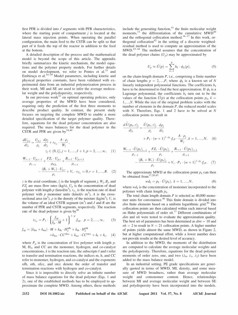
The total chain length domain P is selected as 40,000 mono-mer units for convenience.46 This finite domain is divided intodim finite elements based on a uniform logarithmic grid.40 Thecollocation points are then calculated within each interval basedon Hahn polynomials of order nh.17 Different combinations ofdim and nh were tested to evaluate the approximation quality.The best set of parameters has been determined as dim ¼ 10 andnh ¼ 2 to result in N ¼ 21 collocation points. A higher numberof points yields almost the same MWD, as shown in Figure 2,but at higher computational effort, while a lower number doesnot provide results at the desired level of accuracy.

In addition to the MWD, the moments of the distributionare computed to calculate the average molecular weights andthe polydispersity. Therefore, equations for the dead polymermoments of order zero, one, and two (k0, k1, k2) have beenadded to the mass balance model.

In an industrial setting, PE grade specifications are gener-ally quoted in terms of MWD, MI, density, and some mea-sure of MWD broadness, rather than average molecularweight and comonomer content. Hence, relationshipsbetween MI and average molecular weight and between SEand polydispersity have been incorporated into the models.


The MI measures the weight average molecular weight withan inverse relationship, that is, a higher MI corresponds to alower molecular weight. On the other hand, the SE is a mea-sure for MWD broadness, e.g., a higher SE refers to abroader MWD and hence a higher polydispersity.

Optimization Problem Formulation

The objective of optimization is supposed to reflect some eco-nomic criterion. In batch polymerization, often batch time isminimized or monomer conversion is maximized while con-straining the target average molecular weights and polydisper-sity.8,9 Another very common approach relies on an objectivefunction which combines a number of performance measureswith appropriate weighting factors chosen a priori.10,11 However,the choice of weightings is not always easy because it lacks atransparent conflict resolution. Alternatively, the weighted sumof squares of the deviation of desired monomer conversion andpolymer properties from their specified values has been mini-mized.12,16,17 None of these contributions attempted to target theeconomical performance of the process directly.

Only a few authors employed a truly economic objective inthe optimization, accounting for reactant cost or revenue forexample. O’Driscoll and Ponnuswamy,47 Oliveira et al.,48 andTieu et al.49 consider the initiator cost together with the batchtime in a multiobjective optimization with constraints on poly-dispersity, number average molecular weight and copolymercomposition (when it applies). Zavala and Biegler26 show thatadding polymer production to the objective function improvesthe economic performance of the process.

When the optimization objective only refers to polymerproperties, economically sub-optimal operating conditionsmay be found, since often several operating conditions yieldresins with similar properties. Furthermore, though maximumconversion or minimum batch time are somehow related toprofit, they do not ensure optimal economic operation.Therefore, in the present approach we maximize an eco-nomic profit function given by

U ¼ a �WPE � ðbM �WM þ bH �WH

þ bCAT �WCAT þ bCC �WCC þ bS �WSÞ; ð9Þ

where a is the polyethylene sales price (€/kg), bj represents thecost (€/kg) of raw material j, Wj is a mass flow rate (kg/s) andthe subscripts PE, M, H, CAT, CC, and S denote polyethylene,monomer, hydrogen, catalyst, co-catalyst, and solvent, respec-tively. In industrial practice, the market might demand certainamounts of polymer which can be achieved by constraining thepolymer production rate in the optimization problem. Max-imization of an economic profit function, constrained tomarket demand, leads to optimal conditions with higher profitthan in industrial practice.33 Therefore, better processperformance may be achieved if profit is used as theoptimization criterion, instead of using polymer production,conversion or polymer properties in the objective function.

The decision variables for the series and the parallel pro-cess configurations (s: series; p: parallel), determined by adesign of experiment approach,50 are

us ¼ MT H2;0;T CATT Tin;T H2;1;T z1;T Wt;T Pin;T½ �;(10)

up ¼ MC H2;0;C CATC Ws;C Wt;C Pin;C us½ �; (11)

where M, H2,0, and CAT are monomer, hydrogen, and catalystinlet concentrations, respectively, Tin is the inlet temperature,Wt the total mass flow rate, Pin the inlet pressure, Ws the sidefeed to the CSTR, z1 the lateral hydrogen injection point, H2,1

is the concentration at that point and subscripts C and T referto CSTR and PFRa, respectively. The number of lateralinjection points is (pragmatically) fixed to one a priori, suchthat no discrete variables have to be considered in theoptimization. The total length of PFRa is held constant.33

The desired polymer properties are specified by equalityand inequality constraints at the outlet of the last reactor inthe sequence. The target MWD may be specified by definingn bounds for wdi, i ¼ 1,…,n, n � N. The vector of qualityconstraints at the outlet of PFRb is

h ¼ MI SE wd½ �: (12)

The detailed formulation of the optimization problem isgiven in our previous work33 and is not repeated here. Thestationary mathematical model of the CSTR consists only ofalgebraic equations, whereas the PFR model is represented by

Figure 2. Comparison between different sets of nh and dim.


a differential-algebraic system with the axial coordinate z asindependent variable. A multi-stage model with discontinuitiesalong the spatial coordinates results due to the transitions fromone reactor to the other and due to lateral hydrogen injectionalong the flow path in the PFRa (Figure 1). This multi-stagemodel is solved by integrating along the axial coordinate z.Every PFR model is associated with a finite length spatialinterval while the CSTR models are associated with a spatialinterval with zero length as no differential equations areinvolved. Hence, the CSTR model becomes part of the stagetransition (or the initial) conditions. More precisely, the CSTRmodel enters the initial conditions of PFRb for bothconfigurations (Figure 1).

The multi-stage optimization problem for the series con-figuration (Figure 1a) reads as

maxuk

U (13)

s:t

_xk ¼ fkðxk; yk;uk;p; zÞ; z 2 ½zk�1; zk�; k ¼ 1; ::; J; J þ 2;

(13a)

0 ¼ gkðxk; yk;uk; p; zÞ; z 2 ½zk�1; zk�; k ¼ 1;…; J; J þ 2;

(13b)

0 ¼ x1ðz0Þ � x0; (13c)

Jkð _xk; xk; yk;uk; _xk�1; xk�1; yk�1; uk�1; p; zÞ¼0; k¼2;…; Jþ2;

(13d)

uLB � uk � uUB; (13e)

hLB � h � hUB; z ¼ zf ; (13f)

where x and x are differential state variables and theirderivates with respect to the spatial coordinate z, y thealgebraic state variables, u the decision variables, and p theinvariant parameters. Equation 13c defines the initial condi-tions of the first stage, i.e. the first segment of PFRa. For thefollowing PFR segments k ¼ 2,…,J and k ¼ J þ 2 the initialconditions are determined by the stage transition conditions(13d). The steady-state model of the CSTR relies only on onecompartment and thus does not comprise any differentialequations such that the CSTR model equations can beincorporated into the mapping conditions (13d) for k ¼ J þ1. Here, the partial vectors uk are formed by appropriatesubsets of us (cf., Eq. 10). h are the constraints at the reactoroutlet (cf., Eq. 12).

In the parallel configuration (Figure 1b), if one lateralhydrogen injection point is used, the resulting two segmentsof PFRa define two stages which are represented by nT ¼{1,2}. Note that any other number of injection points can beaccommodated easily. These stages run in parallel with twoother stages denoted by nC ¼ {1,2}, i.e., the CSTR and thePFRb. The mixer constitutes an additional stage nM ¼ {3}which consists only of algebraic equations. The multi-stageoptimal control problem for the parallel configuration istherefore mathematically formulated as:

maxu1

U (14)

s:t:

_xk ¼ fkðxk; yk;uk;p; zÞ; z 2 ½zk�1; zk�; k 2 nT _ nCn 1f g;(14a)

0 ¼ gkðxk; yk;uk;p; zÞ; z 2 ½zk�1; zk�; k 2 nT _ nCn 1f g; (14b)

0 ¼ x1ðz0Þ � x0; (14c)

Jkð _xk; xk; yk; uk; _xk�1; xk�1; yk�1;uk�1; p; zÞ ¼ 0;

k 2 nT _ nC _ nM; ð14dÞuLB � uk � uUB; (14e)

hLB � h � hUB; z ¼ zf ; (14f)

where uk are appropriate subsets of up in Eq. 11 and Jk is theset of algebraic equations that maps the outlet conditions ofstage k-1 to the initial conditions of stage k. Particularly whenk [ nCn{2} or k ¼ 3, Jk is the set of algebraic equations for theCSTR and the mixer. Further details on the formulation of theoptimization problem can be found elsewhere.33

When computing the complete MWD, a more complexoptimization model has to be solved due to the larger num-ber of differential equations and mapping conditions thatarise from the mass balances. If N is the number of colloca-tion points, N differential equations such as (6) have to besolved additionally for each PFR segment, hence (J þ 1) � Nequations in total. The CSTR model adds in turn N algebraicequations such as (7). The same holds true for the mixermodel used in the parallel configuration. Furthermore, foreach stage transition additional N mapping conditions (Eqs.13d and 14d) have to be satisfied. In addition to these differ-ential-algebraic constraints, end-point inequality constraintsare formulated to target the desired polymer properties at thereactor outlet. The solution of the multi-stage optimizationproblem requires a robust and efficient algorithm if themodel predicts the complete MWD.

One possibility to specify a desired MWD is to define thepolymer distribution wdk, k ¼ 1,…,N at every degree of po-lymerization represented by a collocation point. This wouldresult in N additional constraint (Eqs. 13f and 14f) at the re-actor outlet. Our results show however, that the desiredMWD can be satisfactorily predicted and hence specifiedusing, for example, only four collocation points. A moreaccurate specification prediction can be achieved if the dis-tribution’s average and dispersion are additionally set. Wewill show below how different constraint sets can be used tospecify tails at higher chain lengths and even bimodal distri-butions.

The numerical solution of the optimization problem is car-ried out with DyOS, a dynamic optimization software devel-oped and maintained at AVT—Process Systems Engineering,RWTH Aachen University (Germany).51–53

This dynamic optimization software allows for a robustmulti-stage formulation and solution. The multi-stage formu-lation, through its stage transitions, allows the lateral injec-tion points to be modeled as true impulses. Instead of spa-tially discretizing the differential-algebraic equations on afixed grid,25–26 the approach proposed here consists on inte-grating a dynamic model whose independent variable is thespatial coordinate, as mentioned previously. Each stage isthen integrated along a finite length spatial interval so that


the stage lengths can be treated as degrees of freedom allow-ing for an optimal choice of the location of the injectionpoints. In contrast to this late discretization approach, wherethe solution of the spatial differential-algebraic reactor modelis embedded in the optimization problem, Asteasuain andBrandolin25 optimize the steady-state operation of a tubularreactor by means of an early discretization approach. Theirmethod relies on spatial discretization of the tubular reactormodel resulting in a nonlinear programming problem with alarge number of nonlinear algebraic equality constraints,which is solved by the optimization toolbox of gPROMS. Torepresent a hydrogen injection, they add an extra sourceterm to the mass and energy balances valid on the discretiza-tion interval starting at the injection point to approximate animpulse function. The lateral injection point has to be set apriori and cannot be considered as a degree of freedom.

The late multi-stage optimal control approach suggestedhere has several advantages. First, it allows for a preciseconsideration of the location of feed injection points whichconstitutes an important factor influencing the polymer qual-ity. Furthermore, the shooting approach facilitates an accu-rate, error-controlled integration of the differential-algebraicpolymerization model. Hence, the suggested novel problemformulation and solution algorithm outperforms previousmethods with respect to robustness, solution accuracy andcomputational efficiency. In particular, Asteasuain and Bran-dolin25 report that the solution of their optimization problemon a Pentium IV processor running at 3 GHz and using 1GB RAM requires between 2 to 5 h of CPU time while ourmethod solves a typical optimization problem, including thedecision on lateral injection points as part of the optimiza-tion, in only 4 to 20 min on a comparable hardware, i.e., onan Intel Xeon running at 2.66 GHz and using 12 GB RAM.

Another early discretization approach has been recently pro-posed by Zavala and Biegler,26 when targeting LDPE proper-ties (MI and density) in tubular reactors while maintainingpeak temperatures within protection zones. No attempt hasbeen made to either target the whole MWD or to optimize thereactor length and lateral injection points. Their full discretiza-tion formulation is able to handle multi-point boundary condi-tions. Their steady-state reactor model contains about 130 or-dinary differential equations and 500 algebraic equations. Theoptimization model, after full-discretization, covers around13,000 constraints and 71 degrees of freedom.

Table 1 summarizes the computational effort for solving theoptimization problems described in the next section for the se-ries and parallel reactor configurations. The series configura-tion comprises four stages, eight decision variables (Eq. 10),131 differential variables, 3369 algebraic variables, and 33transition conditions between two adjacent stages. The parallelconfiguration consists of three stages, 14 decision variables

(Eq. 11), 165 differential variables, 3513 algebraic variables,and 66 transition conditions between two adjacent stages.

Results and Discussion

Some optimizations runs are presented in this section toillustrate the implementation and the potential of the pro-posed approach for an industrial high density polyethylenereactor. For reasons of confidentiality, all data shown in thefigures and tables have been normalized between 0 and 1.Examples 1 and 2 correspond to the series configuration (cf.Figure 1a), whereas Examples 3 and 4 refer to the parallelconfiguration (cf. Figure 1b).

Usually, in industrial practice the end-use properties arespecified by the customer. A MWD complying with thesespecifications is obtained from laboratory tests (or fromproduct/process knowledge). Some efforts have been madeto develop models correlating end-use properties with theMWD.2–7 If such models are incorporated in the processmodel, the end-use properties could be directly targeted bythe optimization model. In the following case study, the tar-get MWD is specified point-wise at selected molecularweights within a given tolerance (d).

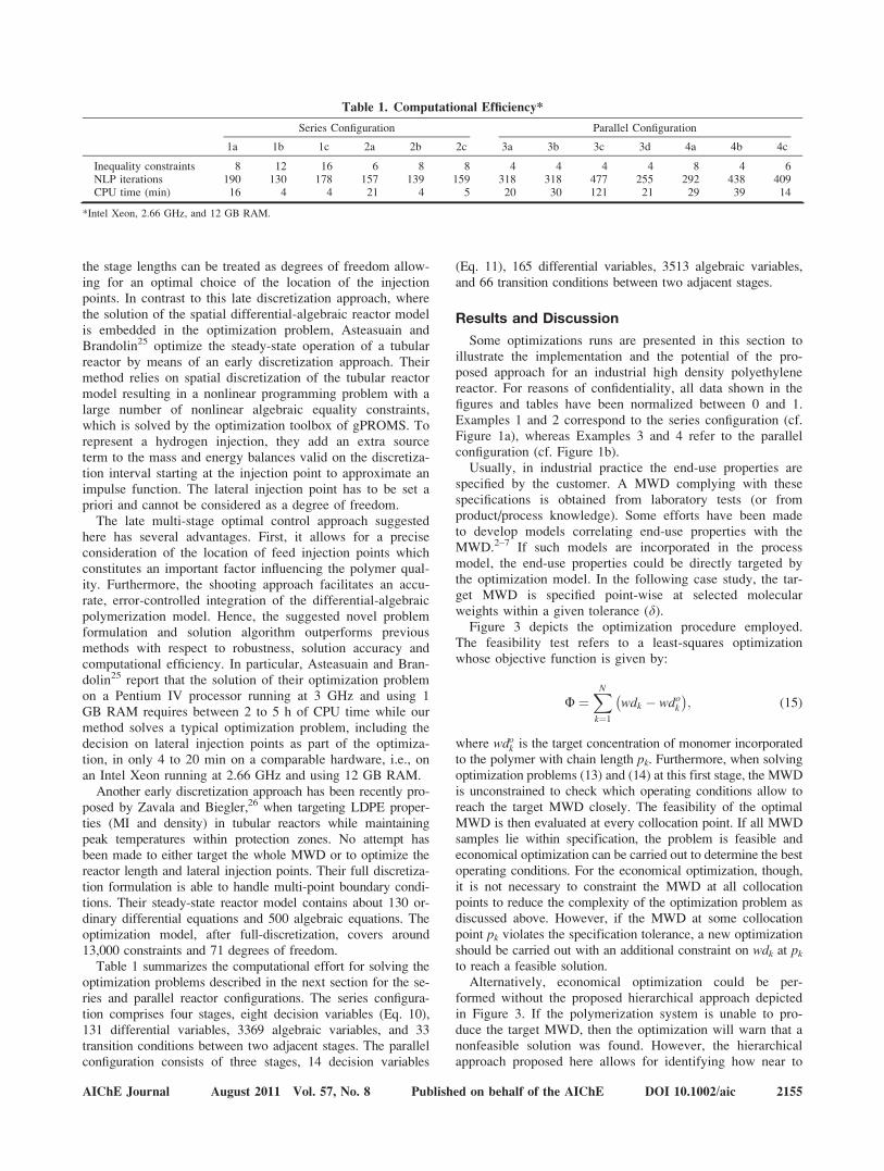
Figure 3 depicts the optimization procedure employed.The feasibility test refers to a least-squares optimizationwhose objective function is given by:

U ¼XN

k¼1

wdk � wdok� �

; (15)

where wdok is the target concentration of monomer incorporatedto the polymer with chain length pk. Furthermore, when solvingoptimization problems (13) and (14) at this first stage, the MWDis unconstrained to check which operating conditions allow toreach the target MWD closely. The feasibility of the optimalMWD is then evaluated at every collocation point. If all MWDsamples lie within specification, the problem is feasible andeconomical optimization can be carried out to determine the bestoperating conditions. For the economical optimization, though,it is not necessary to constraint the MWD at all collocationpoints to reduce the complexity of the optimization problem asdiscussed above. However, if the MWD at some collocationpoint pk violates the specification tolerance, a new optimizationshould be carried out with an additional constraint on wdk at pkto reach a feasible solution.

Alternatively, economical optimization could be per-formed without the proposed hierarchical approach depictedin Figure 3. If the polymerization system is unable to pro-duce the target MWD, then the optimization will warn that anonfeasible solution was found. However, the hierarchicalapproach proposed here allows for identifying how near to

Table 1. Computational Efficiency*

Series Configuration Parallel Configuration

1a 1b 1c 2a 2b 2c 3a 3b 3c 3d 4a 4b 4c

Inequality constraints 8 12 16 6 8 8 4 4 4 4 8 4 6NLP iterations 190 130 178 157 139 159 318 318 477 255 292 438 409CPU time (min) 16 4 4 21 4 5 20 30 121 21 29 39 14

*Intel Xeon, 2.66 GHz, and 12 GB RAM.


the target MWD the process can operate. That makes theoptimization strategy more robust and efficient.

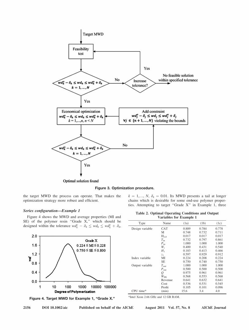
Series configuration—Example 1

Figure 4 shows the MWD and average properties (MI andSE) of the polymer resin ‘‘Grade X,’’ which should bedesigned within the tolerance wdok � dk � wdk � wdok þ dk,

k ¼ 1,…, N, dk ¼ 0.01. Its MWD presents a tail at longerchains which is desirable for some end-use polymer proper-ties. Attempting to target ‘‘Grade X’’ in Example 1, three

Figure 4. Target MWD for Example 1, ‘‘Grade X.’’

Table 2. Optimal Operating Conditions and OutputVariables for Example 1

Type Name (1a) (1b) (1c)

Design variable CAT 0.889 0.784 0.778M 0.748 0.732 0.711H2,0 0.017 0.017 0.017Tin 0.732 0.797 0.861Pin 1.000 1.000 1.000Wt 0.400 0.431 0.540H1 0.183 0.413 0.466z1 0.597 0.929 0.912

Index variable MI 0.224 0.208 0.224SE 0.750 0.740 0.750

Output variable Tout 1.000 1.000 1.000Pout 0.500 0.500 0.500Q 0.975 0.961 0.961WPE 0.568 0.553 0.568Revenue 0.641 0.632 0.641Cost 0.536 0.531 0.545Profit 0.105 0.101 0.096

CPU time* (min) 15.6 3.4 4.0

*Intel Xeon 2.66 GHz and 12 GB RAM.

Figure 3. Optimization procedure.


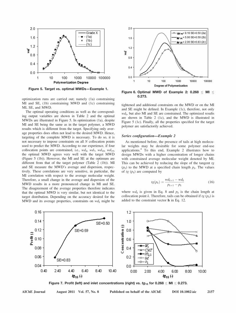
optimization runs are carried out; namely (1a) constrainingMI and SE, (1b) constraining MWD and (1c) constrainingMI, SE, and MWD.

The optimal operating conditions as well as the correspond-ing output variables are shown in Table 2 and the optimalMWDs are illustrated in Figure 5. In optimization (1a), despiteMI and SE being the same as in the target polymer, a MWDresults which is different from the target. Specifying only aver-age properties does often not lead to the desired MWD. Hence,targeting of the complete MWD is necessary. To do so, it isnot necessary to impose constraints on all N collocation pointsused to predict the MWD. According to our experience, if fourcollocation points are constrained, i.e., wd4, wd7, wd10, wd15,the optimal MWD agrees very well with the target MWD(Figure 5 (1b)). However, the MI and SE at the optimum aredifferent from that of the target polymer (Table 2 (1b)). MIand SE measure the MWD’s average and dispersion, respec-tively. These correlations are very sensitive, in particular, theMI correlation with respect to the average molecular weight.Therefore, a small change in the average and dispersion of theMWD results in a more pronounced change in MI and SE.The disagreement of the average properties therefore indicatesthat the optimal MWD is very similar, but not identical to thetarget distribution. Depending on the accuracy desired for theMWD and its average properties, constraints on wdk might be

tightened and additional constraints on the MWD or on the MIand SE might be defined. In Example (1c), therefore, not onlywdk, but also MI and SE are constrained. The optimized resultsare shown in Table 2 (1c), and the MWD is illustrated inFigure 5 (1c). Finally, all the properties specified for the targetpolymer are satisfactorily achieved.

Series configuration—Example 2

As mentioned before, the presence of tails at high molecu-lar weights may be desirable for some polymer end-useapplications.4 To this end, Example 2 illustrates how todesign MWDs with a higher concentration of longer chainswith constrained average molecular weight denoted by MI.This can be achieved by reducing the slope of the tangent tg(pk) to the MWD at a specified chain length pk. The valuesof tg (pk) are computed by

tgðpkÞ ¼ wdkþ1 � wdkpkþ1 � pk

(16)

where wdk is given in Eq. 8 and pk is the chain length atcollocation point k. Therefore, tails can be obtained if tg (pk) isadded to the constraint vector h in Eq. 12.

Figure 5. Target vs. optimal MWDs—Example 1.Figure 6. Optimal MWD of Example 2: 0.268 � MI �

0.273.

Figure 7. Profit (left) and inlet concentrations (right) vs. tg15 for 0.268 � MI � 0.273.


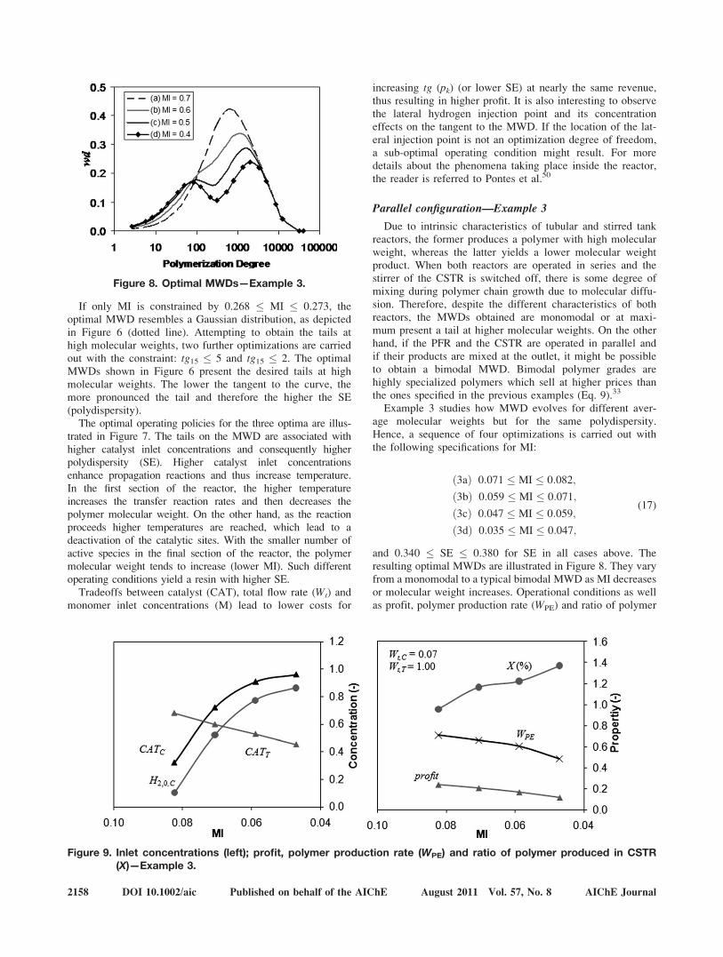
If only MI is constrained by 0.268 � MI � 0.273, theoptimal MWD resembles a Gaussian distribution, as depictedin Figure 6 (dotted line). Attempting to obtain the tails athigh molecular weights, two further optimizations are carriedout with the constraint: tg15 � 5 and tg15 � 2. The optimalMWDs shown in Figure 6 present the desired tails at highmolecular weights. The lower the tangent to the curve, themore pronounced the tail and therefore the higher the SE(polydispersity).

The optimal operating policies for the three optima are illus-trated in Figure 7. The tails on the MWD are associated withhigher catalyst inlet concentrations and consequently higherpolydispersity (SE). Higher catalyst inlet concentrationsenhance propagation reactions and thus increase temperature.In the first section of the reactor, the higher temperatureincreases the transfer reaction rates and then decreases thepolymer molecular weight. On the other hand, as the reactionproceeds higher temperatures are reached, which lead to adeactivation of the catalytic sites. With the smaller number ofactive species in the final section of the reactor, the polymermolecular weight tends to increase (lower MI). Such differentoperating conditions yield a resin with higher SE.

Tradeoffs between catalyst (CAT), total flow rate (Wt) andmonomer inlet concentrations (M) lead to lower costs for

increasing tg (pk) (or lower SE) at nearly the same revenue,thus resulting in higher profit. It is also interesting to observethe lateral hydrogen injection point and its concentrationeffects on the tangent to the MWD. If the location of the lat-eral injection point is not an optimization degree of freedom,a sub-optimal operating condition might result. For moredetails about the phenomena taking place inside the reactor,the reader is referred to Pontes et al.50

Parallel configuration—Example 3

Due to intrinsic characteristics of tubular and stirred tankreactors, the former produces a polymer with high molecularweight, whereas the latter yields a lower molecular weightproduct. When both reactors are operated in series and thestirrer of the CSTR is switched off, there is some degree ofmixing during polymer chain growth due to molecular diffu-sion. Therefore, despite the different characteristics of bothreactors, the MWDs obtained are monomodal or at maxi-mum present a tail at higher molecular weights. On the otherhand, if the PFR and the CSTR are operated in parallel andif their products are mixed at the outlet, it might be possibleto obtain a bimodal MWD. Bimodal polymer grades arehighly specialized polymers which sell at higher prices thanthe ones specified in the previous examples (Eq. 9).33

Example 3 studies how MWD evolves for different aver-age molecular weights but for the same polydispersity.Hence, a sequence of four optimizations is carried out withthe following specifications for MI:

ð3aÞ 0:071 � MI � 0:082;

ð3bÞ 0:059 � MI � 0:071;

ð3cÞ 0:047 � MI � 0:059;

ð3dÞ 0:035 � MI � 0:047;

(17)

and 0.340 � SE � 0.380 for SE in all cases above. Theresulting optimal MWDs are illustrated in Figure 8. They varyfrom a monomodal to a typical bimodal MWD as MI decreasesor molecular weight increases. Operational conditions as wellas profit, polymer production rate (WPE) and ratio of polymer

Figure 8. Optimal MWDs—Example 3.

Figure 9. Inlet concentrations (left); profit, polymer production rate (WPE) and ratio of polymer produced in CSTR(X)—Example 3.


produced in CSTR (X) are shown in Figure 9. For each reactor,all optimal flow rates are the same, but the CSTR operatesalmost at its lower flow rate limit, unlike the tubular reactor.

It is interesting to observe the antagonist behavior of thecatalyst inlet concentration to each reactor in Figure 9. Asmentioned before, lower catalyst concentration leads to lon-ger polymeric chains, i.e., with lower MI. The hydrogen inletconcentration to PFRa is zero for all optimizations, alsoenhancing the formation of longer chains. Therefore, we canconclude that PFRa is responsible for the longer chainswhereas the CSTR contributes to the smaller chains. As theratio of polymer produced in the CSTR increases, the MWDtends to a bimodal distribution as observed in Figure 8.

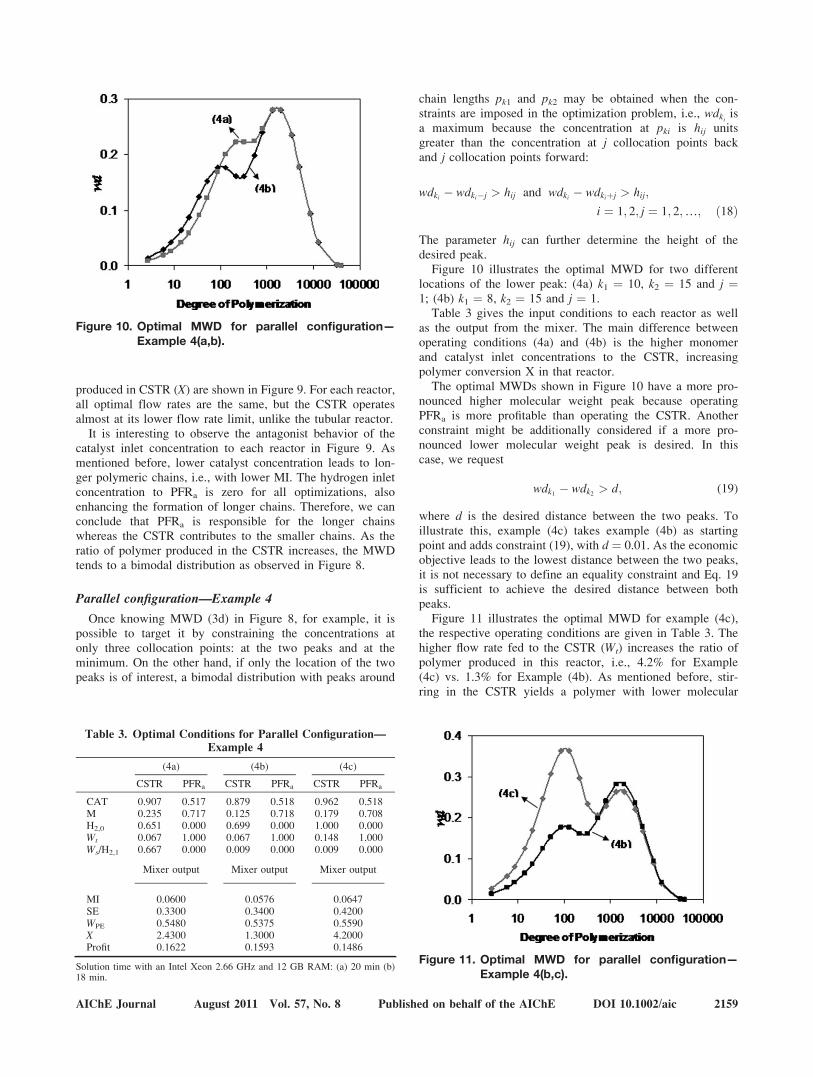
Parallel configuration—Example 4

Once knowing MWD (3d) in Figure 8, for example, it ispossible to target it by constraining the concentrations atonly three collocation points: at the two peaks and at theminimum. On the other hand, if only the location of the twopeaks is of interest, a bimodal distribution with peaks around

chain lengths pk1 and pk2 may be obtained when the con-straints are imposed in the optimization problem, i.e., wdki isa maximum because the concentration at pki is hij unitsgreater than the concentration at j collocation points backand j collocation points forward:

wdki � wdki�j > hij and wdki � wdkiþj > hij;

i ¼ 1; 2; j ¼ 1; 2;…; ð18Þ

The parameter hij can further determine the height of thedesired peak.

Figure 10 illustrates the optimal MWD for two differentlocations of the lower peak: (4a) k1 ¼ 10, k2 ¼ 15 and j ¼1; (4b) k1 ¼ 8, k2 ¼ 15 and j ¼ 1.

Table 3 gives the input conditions to each reactor as wellas the output from the mixer. The main difference betweenoperating conditions (4a) and (4b) is the higher monomerand catalyst inlet concentrations to the CSTR, increasingpolymer conversion X in that reactor.

The optimal MWDs shown in Figure 10 have a more pro-nounced higher molecular weight peak because operatingPFRa is more profitable than operating the CSTR. Anotherconstraint might be additionally considered if a more pro-nounced lower molecular weight peak is desired. In thiscase, we request

wdk1 � wdk2 > d; (19)

where d is the desired distance between the two peaks. Toillustrate this, example (4c) takes example (4b) as startingpoint and adds constraint (19), with d ¼ 0.01. As the economicobjective leads to the lowest distance between the two peaks,it is not necessary to define an equality constraint and Eq. 19is sufficient to achieve the desired distance between bothpeaks.

Figure 11 illustrates the optimal MWD for example (4c),the respective operating conditions are given in Table 3. Thehigher flow rate fed to the CSTR (Wt) increases the ratio ofpolymer produced in this reactor, i.e., 4.2% for Example(4c) vs. 1.3% for Example (4b). As mentioned before, stir-ring in the CSTR yields a polymer with lower molecular

Figure 10. Optimal MWD for parallel configuration—Example 4(a,b).

Table 3. Optimal Conditions for Parallel Configuration—Example 4

(4a) (4b) (4c)

CSTR PFRa CSTR PFRa CSTR PFRa

CAT 0.907 0.517 0.879 0.518 0.962 0.518M 0.235 0.717 0.125 0.718 0.179 0.708H2,0 0.651 0.000 0.699 0.000 1.000 0.000Wt 0.067 1.000 0.067 1.000 0.148 1.000Ws/H2,1 0.667 0.000 0.009 0.000 0.009 0.000

Mixer output Mixer output Mixer output

MI 0.0600 0.0576 0.0647SE 0.3300 0.3400 0.4200WPE 0.5480 0.5375 0.5590X 2.4300 1.3000 4.2000Profit 0.1622 0.1593 0.1486

Solution time with an Intel Xeon 2.66 GHz and 12 GB RAM: (a) 20 min (b)18 min.

Figure 11. Optimal MWD for parallel configuration—Example 4(b,c).


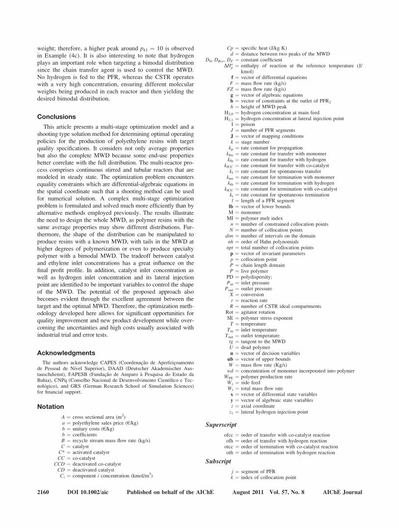
weight; therefore, a higher peak around pk1 ¼ 10 is observedin Example (4c). It is also interesting to note that hydrogenplays an important role when targeting a bimodal distributionsince the chain transfer agent is used to control the MWD.No hydrogen is fed to the PFR, whereas the CSTR operateswith a very high concentration, ensuring different molecularweights being produced in each reactor and then yielding thedesired bimodal distribution.

Conclusions

This article presents a multi-stage optimization model and ashooting type solution method for determining optimal operatingpolicies for the production of polyethylene resins with targetquality specifications. It considers not only average propertiesbut also the complete MWD because some end-use propertiesbetter correlate with the full distribution. The multi-reactor pro-cess comprises continuous stirred and tubular reactors that aremodeled in steady state. The optimization problem encountersequality constraints which are differential-algebraic equations inthe spatial coordinate such that a shooting method can be usedfor numerical solution. A complex multi-stage optimizationproblem is formulated and solved much more efficiently than byalternative methods employed previously. The results illustratethe need to design the whole MWD, as polymer resins with thesame average properties may show different distributions. Fur-thermore, the shape of the distribution can be manipulated toproduce resins with a known MWD, with tails in the MWD athigher degrees of polymerization or even to produce specialtypolymer with a bimodal MWD. The tradeoff between catalystand ethylene inlet concentrations has a great influence on thefinal profit profile. In addition, catalyst inlet concentration aswell as hydrogen inlet concentration and its lateral injectionpoint are identified to be important variables to control the shapeof the MWD. The potential of the proposed approach alsobecomes evident through the excellent agreement between thetarget and the optimal MWD. Therefore, the optimization meth-odology developed here allows for significant opportunities forquality improvement and new product development while over-coming the uncertainties and high costs usually associated withindustrial trial and error tests.

Acknowledgments

The authors acknowledge CAPES (Coordenacao de Aperfeicoamentode Pessoal de Nıvel Superior), DAAD (Deutscher Akademischer Aus-tauschdienst), FAPESB (Fundacao de Amparo a Pesquisa do Estado daBahia), CNPq (Conselho Nacional de Desenvolvimento Cientıfico e Tec-nologico), and GRS (German Research School of Simulation Sciences)for financial support.

Notation

A ¼ cross sectional area (m2)a ¼ polyethylene sales price (€/kg)b ¼ unitary costs (€/kg)b ¼ coefficientsB ¼ recycle stream mass flow rate (kg/s)C ¼ catalyst

C* ¼ activated catalystCC ¼ co-catalyst

CCD ¼ deactivated co-catalystCD ¼ deactivated catalystCi ¼ component i concentration (kmol/m3)

Cp ¼ specific heat (J/kg K)d ¼ distance between two peaks of the MWD

D0, DRor, DF ¼ constant coefficientDHo

p ¼ enthalpy of reaction at the reference temperature (J/kmol)

f ¼ vector of differential equationsF ¼ mass flow rate (kg/s)

FZ ¼ mass flow rate (kg/s)g ¼ vector of algebraic equationsh ¼ vector of constraints at the outlet of PFR2

h ¼ height of MWD peakH2,0 ¼ hydrogen concentration at main feedH2,1 ¼ hydrogen concentration at lateral injection point

I ¼ poisonJ ¼ number of PFR segmentsJ ¼ vector of mapping conditionsk ¼ stage numberkp ¼ rate constant for propagationkfm ¼ rate constant for transfer with monomerkfh ¼ rate constant for transfer with hydrogen

kfCC ¼ rate constant for transfer with co-catalystkf ¼ rate constant for spontaneous transfer

ktm ¼ rate constant for termination with monomerkth ¼ rate constant for termination with hydrogen

ktCC ¼ rate constant for termination with co-catalystkt ¼ rate constant for spontaneous terminationl ¼ length of a PFR segment

lb ¼ vector of lower boundsM ¼ monomerMI ¼ polymer melt indexn ¼ number of constrained collocation pointsN ¼ number of collocation points

dim ¼ number of intervals on the domainnh ¼ order of Hahn polynomialsnpt ¼ total number of collocation pointsp ¼ vector of invariant parametersp ¼ collocation pointP ¼ chain length domainP ¼ live polymer

PD ¼ polydispersity;Pin ¼ inlet pressurePout ¼ outlet pressureX ¼ conversionr ¼ reaction rateR ¼ number of CSTR ideal compartments

Rot ¼ agitator rotationSE ¼ polymer stress exponentT ¼ temperature

Tin ¼ inlet temperatureTout ¼ outlet temperaturetg ¼ tangent to the MWDU ¼ dead polymeru ¼ vector of decision variables

ub ¼ vector of upper boundsW ¼ mass flow rate (Kg/s)wd ¼ concentration of monomer incorporated into polymer

WPE ¼ polymer production rateWs ¼ side feedWt ¼ total mass flow ratex ¼ vector of differential state variablesy ¼ vector of algebraic state variablesz ¼ axial coordinatez1 ¼ lateral hydrogen injection point

Superscript

ofcc ¼ order of transfer with co-catalyst reactionofh ¼ order of transfer with hydrogen reactionotcc ¼ order of termination with co-catalyst reactionoth ¼ order of termination with hydrogen reaction

Subscript

j ¼ segment of PFRk ¼ index of collocation point


M ¼ monomerp ¼ polymer chain lengthr ¼ CSTR ideal zoneU ¼ dead polymer

Greek letters

a ¼ empirical constantb ¼ empirical constantf ¼ linearly independent functionsc ¼ empirical constantkk ¼ dead polymer moment of order kq ¼ medium specific mass (kg/m3)d ¼ tolerance for MWD specification

Literature Cited

1. Kiparissides C. Polymerization reactor modeling: a review of recentdevelopments and future directions. Chem Eng Sci. 1996;51:1637–1659.

2. Costa MCB, Jardini AL, Lima NMN, Embirucu M, Wolf MacielMR, Maciel Filho R. Empirical models for end-use properties pre-diction: application to injection molding of some polyethylene res-ins. J Appl Polym Sci (Print). 2009;114:3780–3792.

3. Latado A, Embirucu M, Mattos A, Pinto JC. Modeling of end-useproperties of poly(propylene/ethylene) resins. Polym Test. 2001;20:419–439.

4. Ariawan AB, Hatzikiriakos SG, Goyal SK, Hay H. Effects of molec-ular structure on the rheology and processability of blow-moldinghigh-density polyethylene resins. Adv Polym Technol. 2001;20:1–13.

5. Hinchliffe M, Montague G, Willis M, Burke A. Hybrid approach tomodeling an industrial polyethylene process. AIChE J. 2003;49:3127–3137.

6. Nele M, Latado A, Pinto JC. Correlating polymer parameters to theentire molecular weight distribution: application to the melt index.Macromol Mater Eng. 2006;291:272–278.

7. Zahedi M, Ahmadi M, Nekoomanesh M. Influence of molecularweight distribution on flow properties of commercial polyolefins.J Appl Polym Sci. 2008;108:3565–3571.

8. Jang SS, Tan DM, Wie IJ. Optimal operations of semi batch solu-tion polymerization of acrylamide with molecular distribution asconstraints. J Appl Polym Sci. 1993;50:1959–1967.

9. Sundaram BS, Upreti SR, Lohi A. Optimal control of batch MMApolymerization with specified time, monomer conversion, and aver-age polymer molecular weights. Macromol Theory Simul. 2005;14:374–386.

10. Zhang JA. Reliable neural network model based optimal controlstrategy for a batch polymerization reactor. Ind Eng Chem Res.2004;43:1030–1038.

11. Curteanu S, Leon F, Galea D. Alternatives for multiobjective opti-mization of a polymerization process. J Appl Polym Sci. 2006;100:3680–3695.

12. Ahn AO, Chang SC, Rhee HK. Application of optimal temperaturetrajectory to batch polymerization reactor. J Appl Polym Sci. 1998;69:59–68.

13. Crowley TJ, Choi KY. Discrete optimal control of molecular weightdistribution in a batch free radical polymerization process. Ind EngChem Res. 1997;36:3676–3684.

14. Crowley TJ, Choi KY. Calculation of molecular weight distributionfrom molecular weight moments in free radical polymerization. IndEng Chem Res. 1997;36:1419–1423.

15. Crowley TJ, Choi KY. Control of molecular weight distribution andtensile strength in a free radical polymerization process. J Appl PolymSci. 1998;70:1017–1026.

16. Sayer C, Araujo PHH, Arzamendi G, Asua JM, Lima EL, Pinto JC.Modeling molecular weight distribution in emulsion polymerizationreactions with transfer to polymer. J Polym Sci Part A: Polym Chem.2001;39:3513–3528.

17. Kiparissides C, Seferlis P, Mourikas G, Morris AJ. Online optimiz-ing control of molecular weight properties in batch free-radical poly-merization reactors. Ind Eng Chem Res. 2002;20:6120–6131.

18. Saliakas V, Chatzidoukas C, Krallis A, Meimaroglou D, KiparissidesC. Dynamic optimization of molecular weight distribution using or-

thogonal collocation on finite elements and fixed pivot methods: anexperimental and theoretical investigation. Macromol React Eng.2007;1:119–136.

19. Vicente M, Sayer C, Leiza JR, Arzamendi G, Lima EL, Pinto JC,Asuaa JM. Dynamic optimization of non-linear emulsion copolymer-ization systems. Open-loop control of composition and molecularweight distribution. Chem Eng J. 2002;85:339–349.

20. Asteasuain M, Soares M, Lenzi MK, Cunningham M, Sarmoria C,Pinto JC, Brandolin A. ‘‘Living’’ free radical polymerization in tu-bular reactors. I. Modeling of the complete molecular weight distri-bution using probability generating functions. Macromol React Eng.2007;1:622–634.

21. Asteasuain M, Soares M, Lenzi MK, Hutchinson RA, CunninghamM, Brandolin A, Pinto JC, Sarmoria C. ‘‘Living’’ radical polymer-ization in tubular reactors, 2 – process optimization for tailor-mademolecular weight distributions. Macromol React Eng. 2008;2:414–421.

22. Brandolin A, Valles EM, Farber JN. High pressure tubular reactorsfor ethylene. Polymerization optimization aspects. Polym Eng Sci.1991;31:381–390.

23. Asteasuain M, Ugrin PE, Lacunza MH, Brandolin A. Effect of mul-tiple feedings in the operation of a high-pressure polymerization re-actor for ethylene polymerization. Polym React Eng. 2001;9:163–182.

24. Cervantes A, Tonelli S, Brandolin A, Bandoni A, Biegler L. Large-scale dynamic optimization of a low density polyethylene plant.Comput Chem Eng. 2002;24:983–989.

25. Asteasuain M, Brandolin A. Modeling and optimization of a high-pressure ethylene polymerization reactor using gPROMS. ComputChem Eng. 2008;32:396–408.

26. Zavala VM, Biegler LT. Large-scale nonlinear programming strat-egies for the operation of ldpe tubular reactors. 18th European Sym-posium on Computer Aided Process Engineering—ESCAPE 18,Lyon, France. 2008.

27. Kiparissides C, Verros G, MacGregor JF. Mathematical modeling,optimization, and quality control of high-pressure ethylene polymer-ization reactors. Polym Rev. 1993;33:437–527.

28. Kiparissides C, Verrosa G, Pertsinidisa A. On-line optimization of ahigh-pressure low-density polyethylene tubular reactor. Chem EngSci. 1994;49:5011–5024.

29. McAuley KB, MacGregor JF. Optimal grade transitions in a gas-phase polyethylene reactor. AICHE J. 1992;38:1564–1576.

30. Chatzidoukas C, Perkins JD, Pistikopoulos EN, Kiparissides C. Opti-mal grade transition and selection of closed-loop controllers in agas-phase olefin polymerization fluidized bed reactor. Chem EngSci. 2003;58:3643–3658.

31. Chatzidoukas C, Pistikopoulos S, Kiparissides C. A hierarchicaloptimization approach to optimal production scheduling in an indus-trial continuous olefin polymerization reactor. Macromol React Eng.2003;3:36–46.

32. Embirucu M, Fontes C. Multi-rate multivariable generalized predic-tive control and its application to a slurry reactor for ethylene poly-merization. Chem Eng Sci. 2006;61:5754–5767.

33. Pontes KV, Maciel R, Embirucu M, Hartwich A, Marquardt W.Optimal operating policies for tailored linear polyethylene resinsproduction. AIChE J. 2008;54:2346–2365.

34. Embirucu M, Lima EL, Pinto JC. Continuous soluble Ziegler-Nattaethylene polymerizations in reactor trains. I. Mathematical modeling.J Appl Polym Sci. 2000;77:1574–1590.

35. Vieira RAM, Embirucu M, Sayer C, Pinto JC, Lima EL. Controlstrategies for complex chemical processes. Applications in polymer-ization processes. Comput Chem Eng. 2003;27:1307–1327.

36. Pinto JC, Oliveira AM Jr, Lima EL, Embirucu M. Data Reconcilia-tion in a Ziegler-Natta ethylene polymerization. Dechema-Monogra-phien. 2004;138:531–535.

37. Embirucu M, Prata DM, Lima EL, Pinto JC. Continuous solubleZiegler-Natta ethylene polymerizations in reactor trains, 2—estima-tion of kinetic parameters from industrial data. Macromol ReactEng. 2008;2:142–160.

38. Embirucu M, Pontes KV, Lima EL, Pinto JC. Continuous solubleZiegler-Natta ethylene polymerizations in reactor trains, 3—influ-ence of operating conditions upon process performance. MacromolReact Eng. 2008;2:161–175.


39. Pontes KV, Cavalcanti M, Maciel Filho R, Embirucu M. Modelingand simulation of ethylene and 1-butene copolymerization in solutionwith a Ziegler-Natta Catalyst. Int J Chem React Eng. 2010; 8:A7.

40. Pontes KV, Maciel R, Embirucu M. An approach for complete mo-lecular weight distribution calculation: application in ethylene coor-dination polymerization. J Appl Polym Sci. 2008;109:2176–2186.

41. Brandolin A, Sarmonia C. Prediction of molecular weight distribu-tions by probability generating functions. Application to industrialautoclave reactors for high pressure polymerization of ethylene andethylene-vinyl acetate. Polym Eng Sci. 2001;41:1413–1426.

42. Villadsen J, Michelsen ML. Solution of Differential Equation Mod-els by Polynomial Approximation. Englewood Cliffs, NJ: PrenticeHall, 1978:446 p.

43. Canu P, Ray WH. Discrete weighted residual methods applied to po-lymerization reactors. Comput Chem Eng. 1991;15:549–564.

44. Neumann CP. Discrete weighted residual methods: a survey. Int JSyst Sci. 1977;8:985–1007.

45. Nele M, Sayer C, Pinto JC. Computation of molecular weight distri-butions by polynomial approximation with complete adaptation pro-cedures. Macromol Theory Simul. 1999;8:199–213.

46. Wulkow M, Deuflhard P. Towards an efficient computational treat-ment of heterogeneous polymer reactions. In: Fatunla SO, editor.Computational Ordinary Differential Equations. Ibadan: UniversityPress Plc, 1992: 287:306.

47. O’Driscoll KF, Ponnuswamy SR. Optimization of a batch polymer-ization reactor at the final stage of conversion. II. Molecular weightconstraint. J Appl Polym Sci. 1990;39:1299–1308.

48. Oliveira AT, Biscaia EC, Pinto JC. Optimization of batch solutionpolymerizations: simulation studies using an inhibitor and a chain-tansfer agent. J Appl Polym Sci. 1998;69:1137–1152.

49. Tieu D, Cluett R, Penlidis A. Optimization of polymerization reactoroperation: review and case studies with the end-point collocationmethod. Polym React Eng. 1994;2:275–313.

50. Pontes KV, Maciel R, Embirucu M. Process analysis and optimiza-tion mapping through design of experiments and its application to apolymerization process. PPS 23—The Polymer Processing Society23rd Annual Meeting, Salvador, 2007.

51. Brendel M, Oldenburg J, Schlegel M, Stockmann K. DyOS usermanual, relase 2.1. Lehrstuhl fur Prozesstechnik, RWTH Aachen,Aachen, Germany, 2002.

52. Oldenburg J, Marquardt W. Disjunctive modeling for optimal con-trol of hybrid dynamic systems. Comput Chem Eng. 2007;32:2346.

53. Schlegel M, Stockman K, Binder T, Marquardt W. Dynamic optimi-zation using adaptative control vector parametrization. ComputChem Eng. 2005;29:1731–1751.

Appendix

This appendix summarizes the kinetic mechanism, the pro-cess model and the polymer property models developed inprevious studies.32–39

The catalyst is a mixture of vanadium and titanium basedcatalysts, activated by triethyl aluminum. The kinetic mecha-nism is described in Table A1.The reactor configuration comprises tubular and stirred

tank reactors modeled by the equations in Tables A2 and A3,respectively. The first PFR is divided into J segments withPFR characteristics, where the starting point of compartment jis located at the lateral mass injection points (Fj). The nonidealCSTR is represented by a sequence of R ideally mixed com-partments in series with backmixing (B) between two adjacentcompartments to represent the mixing inside the reactor. Theside feeds to the CSTR are represented by FZr.Some average polymer properties are related to the MWD

to be used in the optimization of product quality. Thoseproperties include the MI,

MI ¼ a1 � MWw

� ��b1 ; (A1)

and the SE,

SE ¼ 1

a2 þ c2 � exp �b2 � PDð Þ ; (A2)

where ai, bI, and ci are empirical constants determined byEmbirucu et al.34

Table A1. Kinetic Mechanism of Ethylene Copolymerizationby Coordination

Reaction Rate

ActivationCn þ CC ! C*

n kf0 ,n � [Cn]�[CC]Poisoning by impuritiesICC þ CC ! CCD kICC0 � [ICC] � [CC]IC* þ C�

n ! CDn kIC0 � [IC*] � [C�n]

InitiationC�n þ M ! P1,n ki,n � [C�

n] � [M]

PropagationPi;n þM�!kp;n Piþ1;n kp,n � [Pi,n] 7middot; [M]

Spontaneous DeactivationC�n ! CD kd,n � [C�

n]

TransferPi;n þM�!kfm;n P1;n þ Ui kfm,n�[Pi,n]�[M]Pi;n þ H2 �!

kfh;nC�n þUi kfh,n�[Pi,n]�[H2]

Pi;n þ CC�!kfCC;nC�n þ Ui kfCC,n � [Pi,n]�[CC]

Pi;n �!kf ;n

C�n þ Ui kf,n � [Pi,n]

TerminationPi;n þM�!ktm;n CDþ Ui ktm,n � [Pi,n] � [M]Pi;n þ H2 �!

kth;nCDþ Ui kth,n � [Pi,n] � [H2]

Pi;n þ CC�!ktCC;n CDþ Ui ktCC,n � [Pi,n] � [CC]Pi;n �!

kt;nCDþ Ui kt,n � [Pi,n]

Table A2. Mathematical Model of the PFR Compartments

Mass balanceWj þ 1 ¼ Fj þ 1 þ Wj j ¼ 1,2,…, J � 1,

1A � dWj

dzj ¼ 0 ) Wj ¼ constant;

dCi;j

dzj¼ Ci;j

qj� dqjdzj

þ ri;j � A�qjWj; i ¼ 1;…; nc; zj 2 ð0; lj�;

Energy balance

Cpj � Wj

A � dTjdzj¼ �rp;r � DHo

p þMWM � Rr

o

ðCpU � CpMÞdT8>>:

9>>;;

Boundary conditionsCi,j (zj ¼ 0) ¼ C0,i,j, qj(zj ¼ 0) ¼ q0,j, Tj(zj ¼ 0) ¼ T0,j.

Table A3. Mathematical Model of the Nonideal CSTR

Mass balanceWr � 1 þ FZr þ Br þ 1 � Br � Wr ¼ 0 r ¼ 1,…R,

Wr�1 �Ci;r�1

qr�1þ FZr �Ci;r

qFZrþ Brþ1 �Ci;rþ1

qrþ1� ðBrþWrÞ�Ci;r

qrþ Vr � ri;r ¼ 0 i ¼ 1;…; nc;

B1 ¼ 0, BR þ 1 ¼ 0,WP ¼ W0

Energy balance

Pnini¼1 Wi �

Ri

r

CpidT ¼ �Vr � rp;r � DHop þMWM �R

r

0

ðCpU � CpMÞdT8>>>:

9>>>;;

Backmixing model

Br ¼ k�qr�Vr

lr� D0;r þ DRot;r � RotþDF;r � FZr �

Pnrr¼1 FZr þW0

8:

9;�1

8>:

9>;


The conversion and the polymer production rate are com-puted from

X ¼ 100 � k1CM þ k1

(A3)

and

WPE ¼ W

q� k1 �MWM (A4)

respectively, where CM is the monomer concentration, k1 isthe first order dead polymer moment, W the total mass flowrate, MWM is the monomer molecular weight and q the mix-ture density.

Manuscript received Feb. 25, 2010, revision received July 29, 2010, and finalrevision received Sept. 14, 2010.


Documents

Optimal Process Operation for the Production of Linear ... Process Operation for the Production of Linear Polyethylene Resins with Tailored Molecular Weight Distribution ... of a living