Embed Size (px)
Citation preview
Optimal Precautionary Reserves for Low-Income Countries: A Cost-Benefit Analysis
Era Dabla-Norris, Jun Il Kim, and Kazuko Shirono
WP/11/249

© 2011 International Monetary Fund WP/11/249
IMF Working Paper
Strategy, Policy, and Review Department
Optimal Precautionary Reserves for Low-Income Countries: A Cost-Benefit Analysis
Prepared by Era Dabla-Norris, Jun Il Kim, and Kazuko Shirono*
Authorized for distribution by Hugh Bredenkamp
October 2011
Abstract
This paper develops a cost-benefit approach that helps to quantify the optimal level of international reserves in low-income countries, focusing on the role of reserves in preventing and mitigating absorption drops triggered by large external shocks. The approach is applied to a sample of 49 LICs over the period 1980-2008 to yield estimates of the likelihood and severity of a crisis. The calibration results suggest that the standard metric of three months of imports is inadequate for countries with fixed exchange rate regimes. The results also highlight the role of overall policy frameworks and availability of Fund-support in determining optimal reserve levels, raising questions about the uniform applicability of standard rules of thumb across countries.
JEL Classification Numbers: O11, F31, O24
Keywords: Reserve adequacy, optimal level of reserves, low-income countries
Author’s E-Mail Address:[email protected]; [email protected]; [email protected] *This paper was prepared when Jun Il Kim was in the Research Department of the International Monetary Fund. We would like to thank Hugh Bredenkamp, Valerio Crispolti, George Tsibouris, Rex Ghosh, Joshua Aizenman, Oliver Jeanne, Eduardo Levy-Yeyati, and seminar participants at DFID and the SPR seminar series for their useful comments. Ke Wang provided excellent research assistance.
This Working Paper should not be reported as representing the views of the IMF. The views expressed in this Working Paper are those of the author(s) and do not necessarily represent those of the IMF or IMF policy. Working Papers describe research in progress by the author(s) and are published to elicit comments and to further debate.

2
Contents Page
I. Introduction ............................................................................................................................3
II. Reserves in low-Income Countries: Stylized Facts ...............................................................5
III. Analytical Framework .........................................................................................................7
IV. Empirical Analysis ...............................................................................................................9 A. Identifying External Shocks and Crisis Events .........................................................9 B. Estimating the Probability of a Crisis .....................................................................11 C. Cost of a Crisis ........................................................................................................13 D. Robustness Checks ..................................................................................................13
V. Optimal Precautionary Reserves: Calibration Results ........................................................14 A. Benchmark Calibration and Sensitivity Analysis ...................................................14 B. Results across Country Groups ...............................................................................16
VI. Conclusion .........................................................................................................................17 References ................................................................................................................................18 Tables 1. Estimating Reserve Demand in LICs ...................................................................................25 2. Median Growth Rate of Absorption and Consumption, 1990-2009 ....................................26 3. Probability of Absorption Drops ..........................................................................................26 4. Fundamentals and Marginal Effects on Crisis Probability ..................................................27 5. Absorption Loss Regression ................................................................................................27 6. Calibrated Optimal Reserves for Low-Income Countries ...................................................28 Figures 1. Recent Trends in Reserve Accumulation in Low-Income Countries (LICs) .......................20 2. Median Reserve Coverage in Low-Income Countries (LICs) .............................................21 3. Actual and Predicted Reserves, 2002-2008 .........................................................................21 4. External Shock Episodes......................................................................................................23 5. Marginal Effects on the Probability of a Crisis ...................................................................24 6. Sensitivity of Optimal Reserves to Country Fundamentals .................................................24 7. Actual vs. Computed Reserves, 2008-09 .............................................................................25 Appendix Tables A.I Variables Used in Regression Analysis .............................................................................29 A.II Absortpion Drop Probit Regression – Robustness Check ................................................30 A.III Probability of Consumption Drops .................................................................................31 A.IV Absorption Loss Regression – Robustness Check ..........................................................32 A.V Consumption Loss Regression .........................................................................................33 A.VI Sensitivity Analysis of Calibrated Optimal Reserves .....................................................34 A.VII List of Countries in the Sample .....................................................................................35
3
I. INTRODUCTION
Low-income countries are subject to a wide variety of exogenous disturbances—sharp swings in the terms-of trade, export demand, natural disasters, and volatile financial flows—and the resulting high macroeconomic volatility imposes large welfare costs.1 The amplitude, frequency, and economic costs of external shocks tend to be higher than in advanced and emerging market countries (IMF, 2011). International reserves constitute an important form of self-insurance against such shocks, but assessing reserve adequacy in low-income countries has been bedeviled by lack of an agreed methodological framework, with policymakers relying on rules of thumb such as maintaining reserves equivalent to three months of imports to evaluate a country's need. Although such metrics are intuitive and simple, they lack fully developed theoretical and empirical foundations.
This paper seeks to fill this gap by developing a tractable analytical framework that helps to quantify the level of reserves that can be rationalized in terms of insurance against the types of large external shocks faced by low-income countries. We empirically estimate the benefits of reserves in smoothing domestic absorption in response to external shocks. Optimal reserves for different country groups are then calibrated based on the regression estimates, and under simplified assumptions about the cost of holding reserves and the extent of risk aversion.
It is well documented that weakly diversified economic structures and reliance on international trade to import large quantities of essential goods render low-income countries vulnerable to significant fluctuations in consumption in the event of external shocks.2 An event study analysis by Crispolti and Tsibouris (2011) finds that low-income countries with reserve cover more than three months of imports were better able to smooth consumption and absorption in the face of external shocks relative to those with lower coverage. Their analysis also points to the importance of country characteristics and vulnerabilities in assessing reserve adequacy: the shock-mitigation effect of reserves was found to be particularly pronounced, for instance, in highly indebted economies, small islands, commodity exporters, and countries with fixed exchange rate regimes
This paper presents a simple cost-benefit framework of precautionary reserve holdings warranted by country characteristics and fundamentals. The crisis prevention and mitigation benefits of reserves in the event of adverse external shocks—where a crisis is defined as a sharp drop in absorption—are empirically estimated using data on past severe shock episodes for the period 1990-2008, controlling for policy fundamentals and country characteristics.
1 In this paper, “low-income countries” refers to all countries shown on the IMF’s list of countries eligible for the Poverty Reduction and Growth Trust (PRGT) at end-December 2010.
2 See Loayza, Rancière, Servén, and Ventura (2007) and Perry (2009). With so many individuals near subsistence, such declines in consumption can impose very large welfare costs (IMF, 2011).

4
For low-income countries with limited access to international markets, the net financial cost of reserves is implied by foregone investment opportunities or the differential between domestic and foreign real interest rates. The regression estimates for the benefits of holdings reserves are combined with country-specific data on fundamentals, and assumptions about the marginal cost of holding reserves and risk-neutrality to determine optimal reserve levels for different country groups. Our framework explicitly internalizes the interaction between policy fundamentals, access to Fund financing in the event of a shock, and optimal reserve holdings.
The calibration results suggest that the standard metric of reserves equivalent to three months of imports only provides an imprecise benchmark, as optimal reserve holdings depend crucially on country characteristics and policy fundamentals. Calibrated optimal reserves vary from about 1 to 12 months of imports, with higher estimated reserves for fragile states, and commodity exporters than for other countries.3 In addition, optimal reserves are generally higher for fixed exchange rate regimes, in the absence of Fund support in the event of a shock, and for countries facing lower cost of reserves. The calibration results also suggest that stronger policy fundamentals are associated with lower optimal reserve holdings, illustrating the importance of country-specific fundamentals in the determination of optimal reserves.
It is important to note that these estimates constitute a lower bound on the appropriate level of reserves for several reasons. First, given the assumed risk-neutrality in the framework, calibrated reserves are necessarily lower than levels that would emerge under greater risk aversion. Second, countries may accumulate reserves to achieve other objectives beyond self-insurance against external shocks, such as exchange rate policy, or for intergenerational savings.4 These considerations, however, are not directly related to the need for readily available external liquid assets in the event of shocks.
A number of papers have examined the role of reserves as a self-insurance mechanism against external risks. Jeanne and Ranciere (2006, 2008), Aizenman and Lee (2008), Durdu et al. (2009), among others, develop models of optimal reserves for emerging market countries (EMs), in which countries aim to self-insure against sudden-stops in capital inflows. A small number of stylized models have also been developed for low-income countries with limited access to foreign capital markets. These studies primarily focus on risks stemming from the current account. Barnichon (2009) models insurance against natural disasters or terms-of trade shocks, while Drummond and Dhasaman (2008) extend the Jean-Ranciere framework to examine the implications of aid and terms-of-trade shocks.5 The
3 The categorization of fragile states relies on the definition of fragility adopted by the World Bank. 4 For example, countries may also accumulate reserves in order to pursue an export-led growth strategy by artificially maintaining an undervalued exchange rate (Dooley et al., 2004). 5 Valencia (2010) develops a precautionary savings model for optimal reserves for Bolivia. In the face of income uncertainty - represented by the occurrence of current account shocks—agents in the model self-insure
(continued…)

5
optimal level of reserves in these models is highly sensitive to assumptions about the size and probability of external shocks, the potential loss in output and consumption, the opportunity cost of holding reserves, and the degree of risk aversion.
Our contribution to this literature is two-fold. First, we provide empirically-grounded estimates of both the crisis prevention and mitigation benefits of holding reserves against a range of shocks routinely faced by low-income countries. We find that the ratio of reserves to imports is highly statistically significant and of the expected sign in the regressions, even after controlling for other fundamentals, thereby confirming the insurance role of reserves. Moreover, these results are robust across country-samples and time periods. Second, our framework has a more tractable structure, making it easier to calibrate using country-specific data.
The rest of the paper is organized as follows. The next section provides an overview of the recent trends in reserve accumulation in low-income countries. Section III describes the analytical framework, while Section IV presents the results of the empirical analysis. Section V reports the calibration results for optimal reserve levels across country groups; Section VI concludes.
II. RESERVES IN LOW-INCOME COUNTRIES: STYLIZED FACTS
This section provides an overview of recent development in reserve accumulation in low-income countries. We also present results of a reserve demand regression, which allows for a more systematic assessment of reserve adequacy based on peer comparisons.
Figure 1 shows recent trends in reserve accumulation in low-income countries and EMs measured by two traditional metrics, import coverage and as a share of broad money. Import cover is viewed as a measure of the number of months of imports that can be sustained if all external inflows were to cease. Traditionally, three months' coverage is used as a benchmark for import cover. Broad money coverage (typically 20 percent is used as an upper-bound benchmark) provides a measure of the potential for resident-based capital flight and is particularly relevant for dollarized economies and countries with greater capital account openness. As shown in Figure 1, reserve accumulation has generally outpaced traditional reserve adequacy metrics across both country-groups in recent years.6 While the build-up has been slower than in EMs, most low-income countries have accumulated more reserves since by managing a stock of riskless assets to buffer consumption against adverse shocks. Our paper focuses on precautionary reserve holdings rather than precautionary savings, which arise from the inability to mitigate external shocks due to limited and uncertain market access or multilateral/bilateral aid flows. 6 Short-term debt by remaining maturity, another commonly used measure for reserve adequacy in countries that face capital account pressures, is not reported because of the poor quality of short-term external debt data in a large number of low-income countries. For countries with reliable short-term debt data, reserve holdings were found to be significantly above the rule of thumb, reflecting their limited market access and reliance on concessional longer-term financing from official sources.

6
2002 than suggested by the standard rules of thumb, with median coverage ratios of around 4.7 months of imports, and 55 percent of broad money in 2009.
Figure 2 further breaks down reserve accumulation in low-income countries by various country-groups and exchange rate regimes. Since 2003, the ratios of reserves to imports increased most sharply for oil exporters. Sub Saharan African (SSA) countries—a large number of which are commodity exporters—have had persistently higher reserve coverage than the median low-income country, although this difference has narrowed in recent years. On the other hand, reserve coverage in countries with GDP per capita less than US$ 500 has been well-below the low-income country median throughout the 2000s. Finally, recent reserve accumulation has also outpaced the conventional rule of thumb of three months of import cover for both fixed and floating exchange rate regimes, but countries with fixed regimes generally tend to have higher reserve coverage. These aggregate figures mask significant differences across individual countries. As of 2009, over a quarter of all countries had reserve levels lower than suggested by the import cover metric. The accelerating build-up of reserves reflects low initial reserve holdings, increasing openness of economies, a favorable global environment, and policy choice among low-income countries to build precautionary reserves to insure against balance of payment risks.7
To assess whether the recent accumulation in low-income countries has been in line with fundamentals, we estimated a cross-country empirical model of precautionary demand for reserves.8 The basic idea underlying the theory of the reserves demand is that a country chooses a level of reserves to balance the macroeconomic adjustment costs incurred if reserves are exhausted (the precautionary motive) with the opportunity cost of holding reserves. In the multivariate regression, the demand for reserves is modeled as function of the size of the economy and other country fundamentals. The model is estimated using panel data for 62 low-income countries (excluding economies with a population less than 1 million) from 1992 to 2001. The remaining years are used to compare out-of-sample forecasts with actual reserve buildups.
Table 1 reports the regression results for the full sample of low-income countries, and separately for commodity and non-commodity exporters. For the full sample (Column 1), reserve holdings are positively and significantly related to indicators of current account vulnerability (import ratio and export volatility) and indicators of capital account vulnerability, such as broad money. Volatility of the exchange rate and fixed exchange rate regimes are also significantly associated with higher reserve holdings, suggesting that pegged
7 It is also worth noting that the increase in reserves in 2009 is largely attributable to the SDR allocation in response to the global financial crisis. See http://www.imf.org/external/np/sec/pr/2009/pr09283.htm.
8 IMF (2003) and Aizenman and Marion (2002) develop models for EMs. The use of this model for assessing reserve adequacy relies on the assumption that averaged over countries and over the regression sample period there is no systematic bias over under- or over-insurance across countries.
7
countries have greater precautionary demand for reserves than their peers. The proxy for the cost of holding reserves, measured as the interest rate differential between the government treasury bill and the corresponding U.S. asset, is of the expected sign but lacks statistical significance.
The empirical model for the full sample accounts for over 60 percent of the variation in reserves (excluding country fixed effects), suggesting that precautionary motivations are important in explaining average reserve growth across low-income countries. A breakdown of the sample into commodity exporters and non-commodity exporters (Columns 2-3), however, reveals differences between the two groups in accounting for reserve demand. Exchange rate volatility is more important for non-commodity exporters, while export volatility is highly significant in explaining reserves demand in commodity exporters.
How does the reserve buildup in low-income countries between 2002 and 2008 compare with the model’s forecasts? Figure 3 shows a comparison of out-of-sample forecasts derived from the model (Column1 in Table 1) with actual reserve buildups for the 2002-2008 period (excluding the 2009 SDR allocation, which could have distorted reserve holdings). As can be seen in the figure, the growth in low-income country reserve holdings has been broadly in line with evolving fundamentals.
In sum, median reserve accumulation in low-income countries has outpaced standard rules of thumb in recent years. While reserve demand regressions suggest that the recent growth in reserve holdings is largely in line with fundamentals, this analysis does not inform the optimal level of reserves needed in light of the shocks faced by such countries. Instead, the analysis only provides a picture of the determinants of observed reserve holdings. Traditional metrics offer only rough guidance, and, while simple, lack empirical and theoretical foundations. The following sections propose a new approach to assess reserve adequacy in low-income countries using a cost-benefit framework to determine optimal reserve levels.
III. ANALYTICAL FRAMEWORK
Assessing reserve adequacy requires an understanding of the benefits of reserves in smoothing domestic consumption/absorption in response to external shocks. Low-income countries are routinely faced with substantially different shocks than EMs, including sharp swings in foreign aid, remittances, FDI, and natural disasters. While both sets of countries may be affected by shocks to the terms of trade, the frequency and incidence of such shocks tend to be higher in low-income countries (IMF, 2011). Moreover, while crises in EMs are generally characterized by pressures on the capital account, reflecting access to market financing, most low-income countries still have limited access, so that external drains are primarily on the current account. As a result, current-account based measures, such as reserve coverage in months of imports, remain useful indicators of reserve adequacy.
From an insurance perspective, reserves can help reduce the likelihood and magnitude of abrupt drops in consumption and absorption, and consequently a loss in welfare, arising from

8
large fluctuations in imports in the face of large external shocks. As documented by Crispolti and Tsibouris (2011), reserves appear to have cushioned countries against sharp drops in consumption and absorption for a wide range of shocks considered, including during the recent financial crisis. For instance, they find that cumulative consumption losses over a five-year period— measured as yearly loss relative to the pre-shock three-year trend growth— were quite substantial for past external demand and terms-of-trade shocks, at about 6-17 percentage points for countries with reserve coverage of less than three months of imports, whereas the impact was limited among those with higher coverage.
The cost of holding reserves is typically defined as the difference between the return on short-term foreign currency assets and the return on more profitable alternative investment opportunities. The simplicity of this definition, however, masks thorny issues regarding the appropriate definition of alternative investment opportunities.9 For EMs, the net financial cost of holding reserves—the difference between the external funding cost of reserves and the return obtained in relatively safer and more liquid foreign assets—is commonly used as a proxy for the opportunity cost.10
For most low-income countries with limited market access, the net financial cost is likely to be negative since the funding cost, if measured by the concessional interest rate on official borrowing, is typically lower than the return on reserves. Given large infrastructure needs in low-income countries, reserves could alternatively be channeled into productive investment. Hence, a more relevant measure of opportunity cost in these countries is the difference between the return in risky but high-yielding assets, including domestic capital, and safe, low-yielding foreign assets. However, consistent estimates of the marginal product of capital across countries are often not available, and the differential between the domestic and foreign real interest rate is widely used as a proxy.
In what follows, we present a stylized framework that captures the costs and benefits of holding reserves. The objective function that low-income countries seek to maximize reflects the tradeoff between the opportunity cost of holding foreign reserves and the marginal benefit from being able to smooth domestic absorption in the event of large external shocks. Specifically, countries are assumed to maximize the net benefit of holding reserves (NBR):
Max ( , ) ( , )R
NBR q P R Z C R Z r R
9 Indicators identified in the literature include sterilization costs, the differential between domestic and foreign real interest rates, the net financial cost of holding reserves (typically using measure of reserves of sovereign bond spreads), and the opportunity cost of foregone consumption or investment (see Hauner, 2005; Jeanne and Ranciere, 2006). 10 EMs with significant market access (at least during normal times) can, in principle, accumulate reserves by issuing foreign liabilities without affecting net foreign assets or unduly compromising optimal investment or consumption decisions.
(1)

9
Where
P and C represent, respectively, the conditional probability of a crisis given a large shock event and the utility cost of a crisis—where a crisis is defined by a sharp drop in absorption or consumption. Both of these variables depend on reserves R and other control variables Z.
The parameters q and r refer to the unconditional probability of a large shock event and the unit cost of holding reserves, respectively. The first two terms on the right hand side of equation (1) reflect the benefit of holding reserves (in terms of reducing the expected cost of a crisis), while the second term captures the opportunity cost of holding reserves. Given the dependence of the probability and cost of a crisis on Z, the maximization of NBR yields optimal reserves as a function of Z and r.
The specification of NBR reflects the precautionary motive for holding reserves but is subject to several limitations. First, the utility cost is simply measured by the loss in real absorption (in percent of GDP) assuming risk-neutral utility. It is well known that optimal reserves derived from a cost-benefit analysis are particularly sensitive to the assumed degree of risk-aversion in the utility function. In light of this, our framework aims to simulate a lower bound of optimal reserves by assuming linear utility. Assuming risk-neutral utility may also appear at odds with the precautionary motive for holding reserves. But precautionary reserves holdings are not equivalent to precautionary savings, which would not arise under risk-neutral utility. In our analysis, the precautionary motive for holding reserves corresponds to the incentive to guard against the inability to finance large external shocks due to limited market access and uncertain aid flows.
Second, the objective function is static in nature. This is clearly a limitation, but alternative options are likely to be unduly complicated, if not intractable. In the context of low-income countries, assuming a static objective function would not be too unrealistic in light of the fact that other forms of insurance are typically available from multilateral institutions or bilateral donors in case of prolonged shocks.
IV. EMPIRICAL ANALYSIS
In this section, we empirically estimate the conditional probability of a crisis (P) and the cost of a crisis (C) in the event of large external shocks. As a first step, large exogenous shocks and associated crisis events are identified from the data. The absorption smoothing benefits of reserves in the event of shocks are then determined by separately estimating the impact of reserves on the likelihood (P) and the severity of a crisis (C).
A. Identifying External Shocks and Crisis Events
Large negative external shock events in low-income countries are identified if the annual percentage change of the relevant variable falls below the 10th percentile in the left-tail of the country-specific distribution. In particular, shock episodes include one or more of the
10
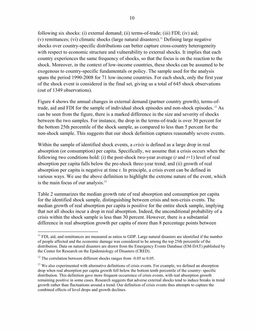
following six shocks: (i) external demand; (ii) terms-of-trade; (iii) FDI; (iv) aid; (v) remittances; (vi) climatic shocks (large natural disasters).11 Defining large negative shocks over country-specific distributions can better capture cross-country heterogeneity with respect to economic structure and vulnerability to external shocks. It implies that each country experiences the same frequency of shocks, so that the focus is on the reaction to the shock. Moreover, in the context of low-income countries, these shocks can be assumed to be exogenous to country-specific fundamentals or policy. The sample used for the analysis spans the period 1990-2008 for 71 low-income countries. For each shock, only the first year of the shock event is considered in the final set, giving us a total of 645 shock observations (out of 1349 observations).
Figure 4 shows the annual changes in external demand (partner country growth), terms-of-trade, aid and FDI for the sample of individual shock episodes and non-shock episodes. 12 As can be seen from the figure, there is a marked difference in the size and severity of shocks between the two samples. For instance, the drop in the terms-of-trade is over 30 percent for the bottom 25th percentile of the shock sample, as compared to less than 5 percent for the non-shock sample. This suggests that our shock definition captures reasonably severe events.
Within the sample of identified shock events, a crisis is defined as a large drop in real absorption (or consumption) per capita. Specifically, we assume that a crisis occurs when the following two conditions hold: (i) the post-shock two-year average (t and t+1) level of real absorption per capita falls below the pre-shock three-year trend; and (ii) growth of real absorption per capita is negative at time t. In principle, a crisis event can be defined in various ways. We use the above definition to highlight the extreme nature of the event, which is the main focus of our analysis.13
Table 2 summarizes the median growth rate of real absorption and consumption per capita for the identified shock sample, distinguishing between crisis and non-crisis events. The median growth of real absorption per capita is positive for the entire shock sample, implying that not all shocks incur a drop in real absorption. Indeed, the unconditional probability of a crisis within the shock sample is less than 30 percent. However, there is a substantial difference in real absorption growth per capita of more than 8 percentage points between
11 FDI, aid, and remittances are measured as ratios to GDP. Large natural disasters are identified if the number of people affected and the economic damage was considered to be among the top 25th percentile of the distribution. Data on natural disasters are drawn from the Emergency Events Database (EM-DAT) published by the Center for Research on the Epidemiology of Disasters (CRED). 12 The correlation between different shocks ranges from -0.05 to 0.05. 13 We also experimented with alternative definitions of crisis events. For example, we defined an absorption drop when real absorption per capita growth fell below the bottom tenth percentile of the country- specific distribution. This definition gave more frequent occurrence of crisis events, with real absorption growth remaining positive in some cases. Research suggests that adverse external shocks tend to induce breaks in trend growth rather than fluctuations around a trend. Our definition of crisis events thus attempts to capture the combined effects of level drops and growth declines.

11
crisis and non-crisis cases, which is also statistically significant. A similar pattern holds for real consumption per capita.
B. Estimating the Probability of a Crisis
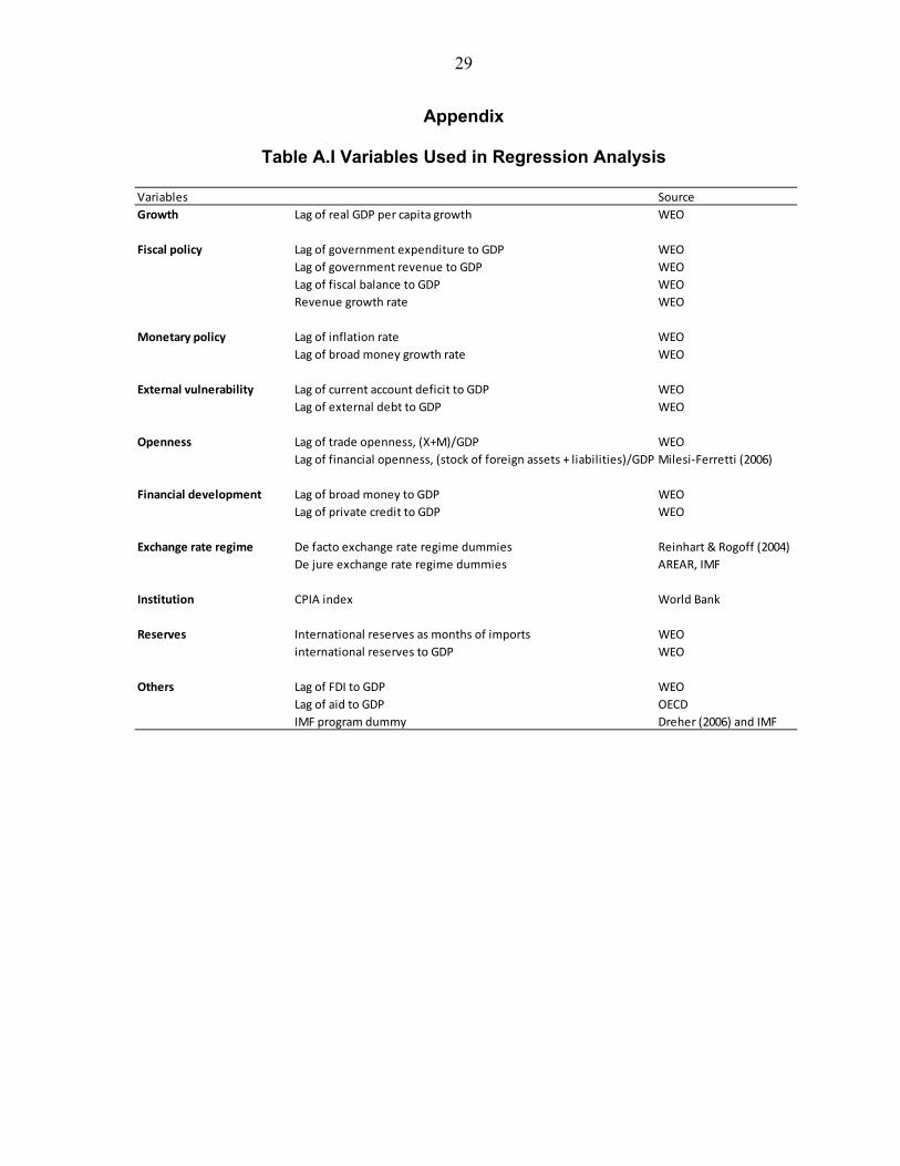
In this sub-section, we estimate the effect of holding reserves on the likelihood of a crisis (a real drop in absorption per capita). A panel probit model is estimated for the conditional probability of a crisis for 49 low-income countries—i.e., the probability of a crisis given a shock—using country characteristics and fundamentals as control variables. The dependent variable is a zero-one binary variable which takes the value of one if a real absorption drop occurs, and 0 otherwise. A general-to-specific approach was used to reach the preferred specification of the model, starting from a set of 21 potential regressors (see Appendix Table I). The final explanatory variables used include reserves (in months of imports), the ratio of government balance to GDP, the World Bank’s CPIA index as a proxy for policy and institutional quality, a dummy for flexible exchange rate regime, and a dummy for Fund-supported programs.14 All explanatory variables are lagged by one year, except for the dummy for Fund-supported programs, and are thus predetermined with respect to the crisis event.15
Table 3 reports the estimation results for absorption drops. The baseline probit regression is reported in column (1). Results from a logit regression (Column 2) and probit regressions for various country groups (Columns 3-6) are also reported for comparison. We find that the probability of a crisis decreases with the quality of a country’s institutions and the ratio of government balance to GDP. Importantly, the coefficient on reserves is of the expected sign, statistically significant, and broadly similar across specifications and estimation methods. These results point to a statistically significant crisis prevention role of reserves and sound fundamentals (such as stronger fiscal position and better institutional quality). The exchange rate regime and Fund support are also important determinants of the likelihood of a crisis, given an external shock. These results are also consistent with the existing view that greater exchange rate flexibility helps facilitate economic adjustment to real shocks (Broda, 2004), and broadly in line with the evidence of the crisis prevention role of Fund-supported programs in emerging markets (Becker et al., 2007).
14 The CPIA is a broad indicator of the quality of a country’s present policy and institutional framework. It is based on 16 criteria which are grouped into four clusters: economic management, structural policies, policy for social inclusion and equity, and public sector management and institutions.
15 Various specifications for the IMF program dummy were considered, including a one-year lag and a combined dummy for lagged and contemporaneous IMF programs. The lagged dummy variable was not statistically significant in any of the specifications. One would expect a positive coefficient for the contemporaneous IMF dummy if there is endogeneity. However, the regression results in Table 3 show a statistically significant negative coefficient for the IMF program dummy, indicating that our results are not due to endogeneity.
12
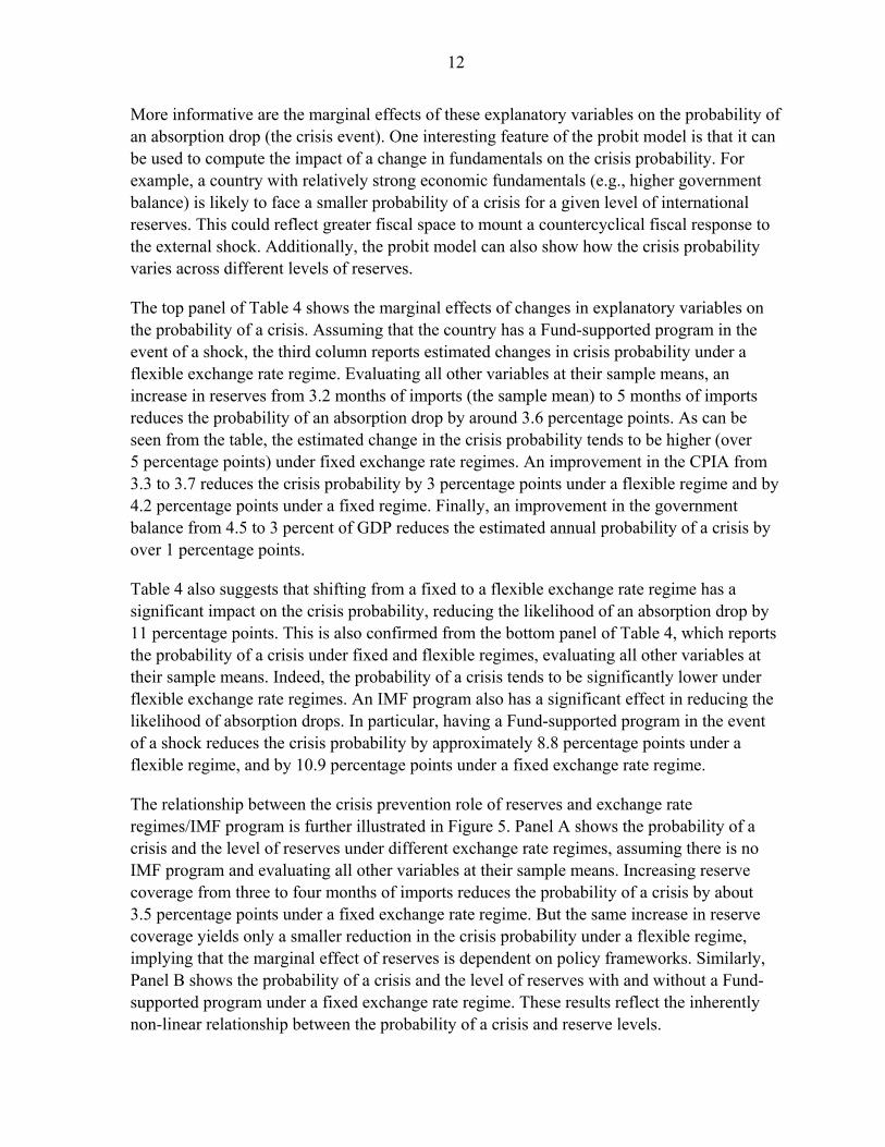
More informative are the marginal effects of these explanatory variables on the probability of an absorption drop (the crisis event). One interesting feature of the probit model is that it can be used to compute the impact of a change in fundamentals on the crisis probability. For example, a country with relatively strong economic fundamentals (e.g., higher government balance) is likely to face a smaller probability of a crisis for a given level of international reserves. This could reflect greater fiscal space to mount a countercyclical fiscal response to the external shock. Additionally, the probit model can also show how the crisis probability varies across different levels of reserves.
The top panel of Table 4 shows the marginal effects of changes in explanatory variables on the probability of a crisis. Assuming that the country has a Fund-supported program in the event of a shock, the third column reports estimated changes in crisis probability under a flexible exchange rate regime. Evaluating all other variables at their sample means, an increase in reserves from 3.2 months of imports (the sample mean) to 5 months of imports reduces the probability of an absorption drop by around 3.6 percentage points. As can be seen from the table, the estimated change in the crisis probability tends to be higher (over 5 percentage points) under fixed exchange rate regimes. An improvement in the CPIA from 3.3 to 3.7 reduces the crisis probability by 3 percentage points under a flexible regime and by 4.2 percentage points under a fixed regime. Finally, an improvement in the government balance from 4.5 to 3 percent of GDP reduces the estimated annual probability of a crisis by over 1 percentage points.
Table 4 also suggests that shifting from a fixed to a flexible exchange rate regime has a significant impact on the crisis probability, reducing the likelihood of an absorption drop by 11 percentage points. This is also confirmed from the bottom panel of Table 4, which reports the probability of a crisis under fixed and flexible regimes, evaluating all other variables at their sample means. Indeed, the probability of a crisis tends to be significantly lower under flexible exchange rate regimes. An IMF program also has a significant effect in reducing the likelihood of absorption drops. In particular, having a Fund-supported program in the event of a shock reduces the crisis probability by approximately 8.8 percentage points under a flexible regime, and by 10.9 percentage points under a fixed exchange rate regime.
The relationship between the crisis prevention role of reserves and exchange rate regimes/IMF program is further illustrated in Figure 5. Panel A shows the probability of a crisis and the level of reserves under different exchange rate regimes, assuming there is no IMF program and evaluating all other variables at their sample means. Increasing reserve coverage from three to four months of imports reduces the probability of a crisis by about 3.5 percentage points under a fixed exchange rate regime. But the same increase in reserve coverage yields only a smaller reduction in the crisis probability under a flexible regime, implying that the marginal effect of reserves is dependent on policy frameworks. Similarly, Panel B shows the probability of a crisis and the level of reserves with and without a Fund-supported program under a fixed exchange rate regime. These results reflect the inherently non-linear relationship between the probability of a crisis and reserve levels.

13
C. Cost of a Crisis
The next step involves estimating the severity of a crisis. Reserves not only help in crisis prevention but also play a role in mitigating the consequences of a crisis. To capture this crisis mitigation role of reserves, we estimate the real absorption loss (normalized in percent of GDP) in the event of external shocks as a function of reserves and other variables. The explanatory variables considered include the log of reserves (in months of import), the exchange rate regime, and the size of shocks.16 The regressions include country fixed effects to control for unobserved cross country heterogeneity. The log of reserves (in months of imports) is used as the relevant dependent variable to capture the non-linearity in the crisis mitigation role of reserves: i.e., the marginal effect of reserves on real absorption loss is diminishing in the level of reserves.17 The inclusion of the size of shocks is necessary to control for the income effect of shocks on real absorption. The regression analysis experimented with other explanatory variables, including a dummy for Fund-supported program, but found them to statistically insignificant. The regressions are estimated over the same sample period and countries used for the probit regressions.
The regression results, summarized in Table 5, support the crisis mitigation role of reserves. Higher reserve holdings are associated with lower absorption losses. The coefficients on the shock variables are of the expected sign (negative as the dependent variable is constructed to be positive to denote a real absorption loss) except for foreign aid shock (which is insignificant in most specifications). The results suggest that positive external demand and terms of trade shocks are associated with lower absorption losses (Column 1). Most striking is the effect of the exchange rate regime. Even after controlling for the size of shocks and including country fixed effects, the regressions suggest that a flexible regime helps reduce real absorption loss by around 9 percent of GDP, relative to the fixed regime. As in previous regressions, these results are largely robust to various sample restrictions, with the estimated coefficients on reserves varying only slightly across various specifications (Columns 2-5 in Table 5).
D. Robustness Checks
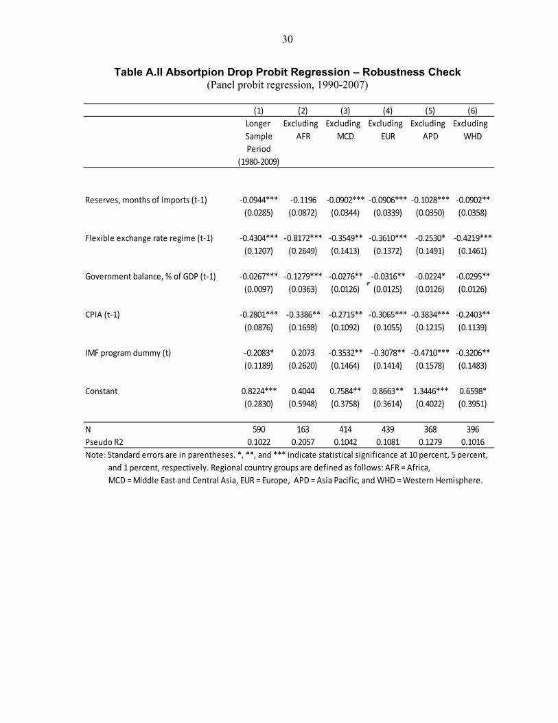
Before moving to the calibration exercise, this subsection briefly discusses various robustness checks for the regressions reported in this section. Appendix Table II reports the robustness of the probit regression across various sub-samples. We find that the reserves variable remains highly significant and of the expected sign, except when the sample is
16 Remittance shocks are not included in the regressions as the number of observations drop substantially if the variable is included in the regression.
17 Alternative specifications were considered for the reserve variable including, R* = R/(1+R). The resulting optimal reserve levels turned out to be very similar to those obtained by assuming a log specification (results available upon request).
14
reduced substantially by dropping African countries. Appendix Table III further reports the probit estimation results using real consumption per capita drops as the relevant dependent variable. The results are similar to those for absorption drops: the coefficients on reserves are statistically significant and of the expected sign, and broadly similar across specifications and estimation methods. These results are also robust across various sub-samples.
Appendix Table IV summarizes the robustness checks for the fixed-effects OLS regressions for absorption loss across various sub-samples. The regression results are again robust to different ways of cutting the sample. In particular, the reserve variable remains significant, with the expected sign across most specifications. Appendix Table V reports robustness checks for the fixed effects OLS regressions with consumption losses as the relevant dependent variable. Reserves and the exchange rate regime are statistically significant and largely robust to different sample restrictions, but other variables are either insignificant or only marginally significant.
In sum, both the probit and the fixed effects OLS regression results are broadly robust to various sample restrictions for both real absorption and consumption per capita. The next section discusses the calibration exercises using the estimated parameters from the absorption regressions.
V. OPTIMAL PRECAUTIONARY RESERVES: CALIBRATION RESULTS
Having estimated conditional probability of a crisis (P) and the cost of a crisis (C), this section elaborates on the calibration results. We first construct a benchmark calibration for various country groups and present some sensitivity analysis. We then present estimates of optimal reserves across different groups and illustrate the relationship with country fundamentals and Fund support.
A. Benchmark Calibration and Sensitivity Analysis
As described in Section III, the behavior of the model economy is determined by four parameters: the conditional probability of a crisis in the event of external shocks P(R, Z), real absorption loss C(R, Z), the unconditional probability of a large shock event (q), and the unit cost of holding reserves (r).This section reports the calibration results for the optimal levels of reserves for various country groups, including ALL (all low-income countries), AFR (Africa), COM (commodity exporters), and FRG (fragile states). Further disaggregation of country groups, albeit desirable in light of significant heterogeneity across low-income countries, was not considered since the number of countries is uneven across country groups, often with too few countries in a certain group to yield statistically meaningful results.
Optimal reserves are calibrated using the estimated conditional probability P(R,Z) and real absorption loss C(R,Z) regression equations reported in the previous section. Other parameter values were taken directly from the data. The unconditional probability of a large shock event (q) is estimated from the data to be 0.5 (the sample average). For the unit cost of

15
holding reserves (r), several reference values were considered, ranging between 2 and 6 percent. These values are based on various existing estimates of the marginal product of capital and the differential between domestic and foreign real interest rates (adjusted for real financial return on reserves of about 1 percent a year).18 Economic fundamentals, such as fiscal balance and the CPIA index are set to their respective five-year average over the period of 2003-07 for each country group.
Shock values in the calibration are taken from the sample median for different country groups.19 The estimated real absorption loss (for chosen values of shocks and country fundamentals) is augmented by one standard deviation of the residuals from the fixed effects OLS absorption loss regression. Assuming normality, the augmented value corresponds roughly to the upper 85th percentile of the distribution of absorption losses. Given that there remains large unexplained variation in the fixed effects OLS absorption loss regression (the regression accounts for 35 percent of the variation in absorption loss across countries), this adjustment is intended as an attempt to capture possible risk aversion.20
The calibration assumes the availability of access to (contingent) IMF support in the event of large external shocks, which affects the conditional probability of a crisis.21 Calibrated optimal reserves are reported in Table 6 for different country groups. As can be seen from the table, these vary from less than 2 to over 12 months of imports depending on country characteristics, fundamentals, and the cost of holding reserves. In all instances, optimal reserves are generally higher for countries with fixed exchange rate regimes, and for fragile states and commodity exporters, reflecting their greater vulnerability to external shocks.
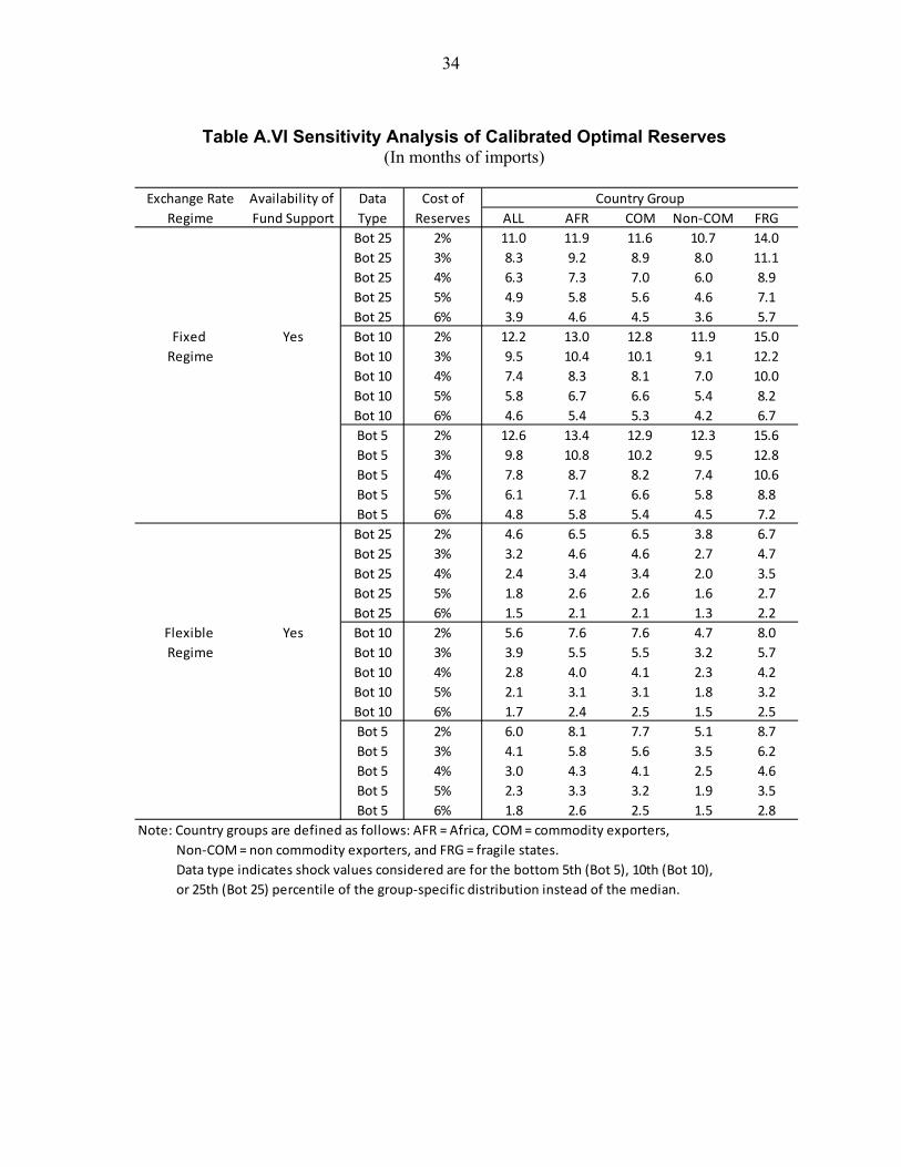
Sensitivity analysis undertaken for the calibration results suggests that optimal reserves are higher if more extreme shock values are considered (taking the bottom 5th, 10th or 25th percentile of the group-specific distribution instead of the median—See Appendix Table VI) For example, assuming that the unit cost of holding reserves is 4 percent, optimal reserves for 18 The marginal product of capital is an important measure for LICs given their large investment needs. Caselli and Freyer (2007) calculate a range of 3 to 8 percent for the marginal product of capital in low-income countries.
19 Alternatively, shock values could be simulated by assuming a multivariate normal distribution for shocks, with the variance-covariance matrix estimated from the sample. Optimal reserves could then be calibrated for each set of simulated shock values, and then averaged to yield final results. While computationally demanding, this option allows for explicitly accounting for the correlation among shocks.
20 In view of the large uncertainty surrounding estimates of risk-aversion parameters, experimenting with more extreme shock values or larger adjustments while assuming risk-neutral utility, could be a practical approach to address differences in the risk attitude across countries.
21 Since a large shock event is defined as a union of six individual shock events (defined at or below the 10th percentile of the country-specific sample distribution), the unconditional probability q should be close to 0.6 if individual shocks are uncorrelated. The sample estimate of 0.5 thus suggests that individual shocks are positively (albeit weakly) correlated in the sample.

16
commodity exporters are 3.4 months of import under the flexible regime if shock values were set to the 25th percentile instead of the median. Similarly, as can be seen from Table 6, optimal reserve levels are sensitive to assumptions about the unit cost of holding reserves.
B. Results across Country Groups
As discussed above, calibrated optimal reserves vary depending on country characteristics and the cost of holding reserves. While the range of calibrated optimal reserves encompasses the traditional rule of thumb of 3 months of imports, the results suggest that this benchmark is more appropriate for countries with flexible exchange rate regimes—particularly if Fund support is readily available. It should be emphasized, however, that the calibration assumes risk-neutral utility and thus tends to yield a lower bound of optimal reserves. As such, the traditional rule of thumb is likely to be inadequate for countries with fixed exchange rate regimes. For the representative low-income country, assuming the unit cost of holding reserves is set at 4 percent, the “insurance” value of a flexible exchange rate regime—measured in terms of annual savings in the cost of holding optimal reserves—is about 0.6 percent of GDP per year (or around three months of imports on average). A similar calculation suggests that the availability of (contingent) Fund support can result in annual savings in optimal reserves of about 0.3 percent of GDP per year (around two months of imports), and could possibly be higher.
The overall policy framework plays an important role in the determination of optimal reserve levels. Figure 6 illustrates the sensitivity of calibrated optimal reserves to various country fundamentals for low-income countries in Sub Saharan Africa when the unit cost of holding reserves is set at 4 percent. It is evident that a stronger fiscal position is associated with lower optimal reserves. Similarly, better policy and institutional frameworks, as measured by a higher CPIA score, are also associated with lower optimal reserves. The results also suggest that the sensitivity of optimal reserves to varying fundamentals differs across exchange rate regimes, with a higher sensitivity for fixed regimes. This result underscores the importance of country-specific fundamentals in the determination of optimal reserves. As such, this suggests that applying a uniform metric for reserve adequacy across all low-income countries could be inappropriate.
An assessment of actual reserve holdings against the derived optimal reserves suggests that, on average, low-income country reserve holdings are broadly adequate. Figure 7 shows a comparison of actual reserve holdings in low-income countries against computed optimal reserve levels. Based on end-2008 data, low-income countries with fixed exchange rate regimes, particularly commodity exporters and fragile states, were, on average, below the computed adequacy range. Countries with flexible regimes were well above the range, although this masks significant differences across individual countries. A comparison of optimal reserves with end-2009 data shows a slightly different picture as the 2009 SDR allocation likely distorted reserve holdings for many low-income countries. A number of caveats should be borne in mind while drawing inferences from this comparison: countries with flexible regimes are relatively more open and integrated with international financial

17
markets as compared to other low-income countries, suggesting that capital flight risks may be playing a role; other non-precautionary motives for holding reserves, including monetary policy and exchange rate decisions by the central bank, could also be pertinent for managed float regimes.
VI. CONCLUSION
This paper presents a simple cost-benefit approach for the optimal level of reserves in low-income countries, based on the assumption that the main benefit of reserves is to smooth domestic absorption/consumption against the disruption induced by large exogenous shocks. The role of reserves in reducing the probability and severity of sudden stops is robustly established through regression analysis.
The calibration exercise shows that the optimal reserves level can be sensitive to country fundamentals and exchange rate regimes, and the model needs to be carefully calibrated to evaluate each country’s needs. As a result, rules of thumb such as maintaining reserves equivalent to three months of imports can only give imprecise benchmarks. Our paper further suggests that reserves only provide a temporary and partial solution to the vulnerabilities that stem from low-income countries’ lack of economic diversification and weak policy and institutional frameworks. To durably reduce risks, countries need to implement economic reforms that address these issues directly. Accordingly, strengthening policy frameworks, increasing exchange rate flexibility, and diversifying economies, could result in declining reserve needs in line with ensuing reductions in external vulnerability.
Two directions would seem especially interesting for extending our framework in future work. First, we would like to have better estimates of the cost of holding reserves in low-income countries. In this respect, future work could focus on obtaining consistent estimates of the marginal product of capital across low-income countries. This would provide a better gauge of the opportunity cost of holding reserves. Second, it would be interesting to examine issues related to optimal reserve levels in currency unions. Such analysis would ideally need to take into account the institutional features and requirements of the currency union arrangement.
18
References Aizenman, Joshua, and Nancy Marion, 2003, "The high demand for international reserves in
the Far East: What is going on?" Journal of the Japanese and International Economies, Vol. 17(3), pp. 370-400.
Aizenman, Joshua, and Jaewoo Lee, 2008, "Financial versus Monetary Mercantilism: Long-run View of Large International Reserves Hoarding," The World Economy, Vol. 31(5), pp. 593-611.
Barnichon, Regis, 2009, “The Optimal Level of Reserves for Low-Income Countries: Self-Insurance against External Shocks,” IMF Staff Papers, Vol.56 (4), pp. 852-875.
Becker, Törbjörn I., Olivier Jeanne, Paolo Mauro, Jonathan David Ostry, and Romain Ranciere, 2007, “Country Insurance: The Role of Domestic Policies,” Occasional Paper No. 254 (Washington: International Monetary Fund).
Broda, Christian, 2004, "Terms of Trade and Exchange Rate Regimes in Developing Countries," Journal of International Economics, Vol. 63, pp. 31-58.
Caselli, Franceso, and James Feyrer, 2007, “The Marginal Product of Capital,” Quarterly Journal of Economics, 122, pp. 535-568.
Crispolti, Valerio, and George Tsibouris, 2011, “International Reserves in Low Income Countries: An Event Study Analysis,” IMF Working Paper, forthcoming (Washington: International Monetary Fund).
Dooley, Michael P., David Folkerts-Landau, and Peter Garber, 2004, "The Revised Bretton Woods System," International Journal of Finance and Economics, Vol. 9, pp.307-313.
Dreher, Axel, 2006, “IMF and Economic Growth: The Effects of Programs, Loans, and Compliance with Conditionality,” World Development, Vol. 34, pp.769-788.
Drummond, Paulo, and Anubha Dhasmana, 2008, "Foreign Reserve Adequacy in Sub-Saharan Africa," IMF Working Papers 08/150 (Washington: International Monetary Fund).
Durdu, Ceyhun Bora, Enrique Mendoza, and Marco Terrones, 2009, "Precautionary Demand for Foreign Assets in Sudden Stop Economies: An Assessment of the New Mercantilism," Journal of Development Economics, Vol. 89, pp. 194-209.
Hauner, David, 2006, "A Fiscal Price Tag for International Reserves," International Finance, Vol. 9(2), pp. 169-195.
International Monetary Fund, 2003, World Economic Outlook. Available at http://www.imf.org/external/pubs/ft/weo/2003/02/
International Monetary Fund, 2011, “Managing Volatility: A Vulnerability Exercise for Low-Income Countries.” Available at www.imf.org/external/np/pp/eng/2011/030911.pdf.
Loayza, Norman V., Romain Rancière, Luis Servén, and Jaume Ventura, 2007, “Macroeconomic Volatility and Welfare in Developing Countries: An Introduction,” World Bank Economic Review, Oxfort University Press, Vol. 23(3), pp.343-357.
19
Perry, Guillermo, 2009, “Beyond Lending: How Multilateral Banks Can Help Developing Countries Manage Volatility” (Washington: Center for Global Development).
Ranciere, Romain, and Oliver Jeanne, 2006, “The Optimal Level of International Reserves for Emerging Market Countries: Formulas and Applications,” IMF Working Paper 06/229 (Washington: International Monetary Fund).
Ranciere, Romain, and Oliver Jeanne, 2008, “The Optimal Level of International Reserves for Emerging Market Economies: A New Formula and Some Applications,” CEPR Discussion Papers No. 6723.
Valencia, Fabian, 2010, “Precautionary Reserves: An Application to Bolivia,” IMF Working Papers 10/54 (Washington: International Monetary Fund).

20
Figure 1. Recent Trends in Reserve Accumulation in Low-Income Countries (LICs) and Emerging Market Economies (EMs)
(Median reserve holdings)
Source: World Economic Outlook
0
1
2
3
4
5
6
19
91
19
93
19
95
19
97
19
99
20
01
20
03
20
05
20
07
20
09
Reserves in Months of Imports
3 Months of Imports
EMs
LICs
0
10
20
30
40
50
60
19
91
19
93
19
95
19
97
19
99
20
01
20
03
20
05
20
07
20
09
Reserves to Broad Money,(in percent)
20 Percent of Broad Money
EMs
LICs

21
Figure 2. Median Reserve Coverage in Low-Income Countries (LICs) (in months of current year's imports)
Source: World Economic Outlook
0
1
2
3
4
5
6
7
8
1990 1993 1996 1999 2002 2005 2008
Oil exporters
LICs
0
1
2
3
4
5
6
1990 1993 1996 1999 2002 2005 2008
Oil importers
LICs
0
1
2
3
4
5
6
1990 1993 1996 1999 2002 2005 2008
SSA
LICs
0
1
2
3
4
5
6
1990 1993 1996 1999 2002 2005 2008
GDP per capita less than US$500
LICs
0
1
2
3
4
5
6
1990 1993 1996 1999 2002 2005 2008
de facto fixed exchange regime in 2007
LICs
0
1
2
3
4
5
6
1990 1993 1996 1999 2002 2005 2008
de facto floating exchange regime in 2007
LICs

22
Figure 3. Actual and Predicted Reserves, 2002-2008 (mean, in percent of GDP)
Sources: World Economic Outlook and staff estimates.
0
5
10
15
20
20
02
20
03
20
04
20
05
20
06
20
07
20
08
ActualPredicted

23
Figure 4. External Shock Episodes
Source: Staff estimates.
-7 -6 -5 -4 -3 -2 -1 0 1 2
Aid (change in the ratio to GDP)
25th percentile 50th percentile 75th percentile
Shock episode
Non-shock episode
-6 -4 -2 0 2
FDI
(change in the ratio to GDP)
25th percentile 50th percentile 75th percentile
Shock episode
Non - shock episode
-40 -30 -20 -10 0 10
Terms of trade
(percentage change)
25th percentile 50th percentile 75th percentile
Shock episode
Non-shock episode
0 1 2 3 4 5
External demand(percentage change)
25th percentile 50th percentile 75th percentile
Shock episode
Non- shockepisode

24
Figure 5. Marginal Effects on the Probability of a Crisis
Source: Staff estimates.
Note: Government balance and CPIA are assumed to be at their respective mean values. Panel A assumes no Fund-supported program; Panel B assumes the fixed exchange rate regime.
Figure 6. Sensitivity of Optimal Reserves to Country Fundamentals
0
5
10
15
20
25
30
35
40
45
50
1 2 3 4 5 6 7 8 9 10
Pro
bab
ility
of
ab
so
rptio
n d
rop
Reserves, months of imports
A. Reserves and Exchange rate Regimes
Fixed regime
Flexible regime
10
15
20
25
30
35
40
45
50
1 2 3 4 5 6 7 8 9 10
Pro
bab
ility
of
ab
so
rptio
n d
rop
Reserves, months of imports
B. Reserves and IMF Program
No IMF program
IMF program
0
1
2
3
4
5
6
7
8
9
-10.0 -5.0 0.0 5.0 10.0
Op
tima
l Re
serv
es
(mo
nth
s o
f im
po
rts)
Fiscal Balance (% of GDP)
Optimal Reserves and Fiscal Balance
Fixed regime
Flexible regime
0123456789
101112
1.0 2.0 3.0 4.0 5.0
Op
tima
l Re
serv
es
(mo
nth
s o
f im
po
rts)
CPIA
Optimal Reserves and CPIA
Fixed regime
Flexible regime

25
Figure 7. Actual vs. Computed Reserves, 2008-09
Notes: The calculation assumes access to Fund-support following a shock.
Country groups are as follows: SSA = Africa, COM = commodity exporters, FRG = fragile states.
Optimal reserves are calculated assuming that the cost of holding reserves is 4 percent. A range
of optimal reserves is also shown with the cost of reserves varying from 3 to 5 percent.
Table 1. Estimating Reserve Demand in LICs
0
2
4
6
8
10
12
ALL SSA COM FRG
Op
tim
al R
ese
rve
s ( m
on
ths
of im
port
s)
Fixed Regime
Optimal ReservesActual Reserves 2009Actual Reserves 2008
0
1
2
3
4
5
6
7
ALL SSA COM FRG
Op
tim
alR
ese
rve
s (m
on
ths
of
imp
ort
s)
Flexible Regime
All LICs Commodity Non-Commodity
Exporters Exporters
VARIABLES (1) (2) (3)
Income -0.0045*** -0.0051*** -0.0049***
(0.0006) (0.0009) (0.0008)
Log(Population) -2.2280*** -0.9651 -2.7470***
(0.3743) (0.6741) (0.4570)
Imports/GDP 0.2611*** 0.1758*** 0.2783***
(0.0198) (0.0361) (0.0230)
Exchange rate volatility -0.0351** -0.0092 -0.1334**
(0.0147) (0.0164) (0.0639)
Export volatility (3y st. dev.) 0.0482** 0.0930*** -0.0367
(0.0235) (0.0340) (0.0333)
Broad Money/GDP 0.3374*** 0.5694*** 0.3077***
(0.0326) (0.0617) (0.0394)
Peg Dummy 1.2851* 0.0731 0.8605
(0.7792) (1.4817) (0.9293)
Interest rate differential with US -0.2178 -0.2172 -0.579
(0.5248) (0.7717) (0.6832)
Observations 414 140 274
R-squared 0.639 0.707 0.668
Note: Dependent variable is Reserves/GDP; all regressions include a constant term.
Standard errors are in parentheses; *, **, and *** indicate statistical significance at 10 percent,
5 percent, and 1 percent, respectively.
Explanatory variables are defined as follows: Income is GDP per capita; Exchange rate volatility is
the moving average of three year standard deviation of monthly exchange rate growth;
Export volatility is the moving average of three year standard deviation of annual export growth rate;
Peg dummy is a dummy which takes the value of one when a country has fixed exchange
rate regime; Interest rate differential with US is the difference between the government treasury
bill and the corresponding U.S. asset.
1992-2001

26
Table 2. Median Growth Rate of Absorption and Consumption, 1990-2009 (Percent, otherwise indicated)
Table 3. Probability of Absorption Drops (Panel probit regression, 1990-2007)
Sample
All Shock Crisis No Crisis Probability
Episodes Episodes Episodes of Crisis
Absorption
1.4 -5.2 3.2 27.1
Obs. 446 121 325
Consumption
1.1 -4.6 2.8 29.1
Obs. 446 130 316
Note: The sample period is 1990-2009. The median growth rate is computed
using observations for which all explanatory variables used in the probit
regression are available.
Growth Rate
(1) (2) (3) (4) (5) (6)
Baseline Logit Excluding Excluding Excluding Excluding
Probit Fragile Commodity Oil Island
States Exporters Exporters Economies
Reserves, months of imports (t-1) -0.0896*** -0.1556*** -0.1018** -0.1333*** -0.0949*** -0.0734**
(0.0339) (0.0595) (0.0490) (0.0446) (0.0357) (0.0354)
Flexible exchange rate regime (t-1) -0.3801*** -0.6568*** -0.1392 -0.5043*** -0.4106*** -0.3884***
(0.1366) (0.2340) (0.1779) (0.1700) (0.1400) (0.1492)
Government balance, % of GDP (t-1) -0.0323*** -0.0537** -0.0175 -0.0312** -0.0343*** -0.0363***
(0.0125) (0.0220) (0.0169) (0.0149) (0.0132) (0.0138)
CPIA index (t-1) -0.3090*** -0.5129*** -0.3805* -0.4028*** -0.3245*** -0.2560**
(0.1056) (0.1766) (0.2080) (0.1209) (0.1083) (0.1256)
IMF program (t) -0.3021** -0.5223** 0.1042 -0.1440 -0.2820* -0.3642**
(0.1409) (0.2374) (0.2016) (0.1741) (0.1453) (0.1561)
Constant 0.8648** 1.4790** 0.7844 1.2357*** 0.9175** 0.6974*
(0.3614) (0.6039) (0.7989) (0.4296) (0.3803) (0.4130)
No. of observation 445 445 282 311 427 385
Pseudo R2 0.1099 0.1103 0.0457 0.1431 0.1105 0.1080
Note: Standard errors are in parentheses. *, **, and *** indicate statistical significance at 10 percent, 5 percent,
and 1 percent, respectively. The categorization of fragile states relies on the definition of fragility adopted
by the World Bank.
Absorption

27
Table 4. Fundamentals and Marginal Effects on Crisis Probability (Percentage point, unless otherwise indicated)
Table 5. Absorption Loss Regression (FE regression with the probit sample)
Fundamentals Sample mean Parameter change Flexible exchange rate Fixed exchange rate
Reserves, months of imports 3.2 3.2 --> 5 -3.6 -5.1
Government balance, % of GDP -4.5 -4.5 --> -3 -1.1 -1.6
CPIA index 3.3 3.3-->3.7 -3.0 -4.2
IMF program dummy no program --> program -8.8 -10.9
Exchange rate regime dummy fixed --> flexible -11.1
Evaluated at mean value, percent
Probability of crisis (no IMF program ) 25.2 38.5
Probability of crisis (with IMF program) 16.5 27.6
Estimated change in crisis probability with IMF program
(1) (2) (3) (4) (5)
Baseline Excluding Excluding Excluding Excluding
Fragile Commodity Oil IslandExporters Exporters Economies
Log of reserves, months of imports (t-1) -2.2403*** -2.0268* -1.5548** -2.0425*** -2.5021***
(0.6677) (1.1416) (0.6324) (0.6634) (0.7306)
Flexible exchange rate regime (t-1) -8.6983*** -8.4203** -5.6632** -8.6269*** -7.8198***
(2.1689) (3.3245) (2.2809) (2.2192) (2.5429)
External demand growth (t) -0.9320** -1.1587* -0.8478** -0.8066* -0.5799
(0.4356) (0.6734) (0.4294) (0.4242) (0.4415)
Terms of trade growth (t) -0.0841* -0.0704 0.0072 -0.0732 -0.1193**
(0.0484) (0.0431) (0.0226) (0.0478) (0.0561)
Change in FDI to GDP (t) -0.0159 0.6605** -0.7468 0.1236 -0.1136
(0.3391) (0.2762) (0.4908) (0.4551) (0.3237)
Change in aid to GDP (t) 0.0527 0.2125 0.0941 0.0615 0.0427
(0.0839) (0.2199) (0.1081) (0.0855) (0.0904)
N 418 264 287 401 360
Adjusted R2 0.34 0.37 0.47 0.34 0.33
Country fixed effects Yes Yes Yes Yes Yes
Note: Robust standard errors are in parentheses. *, **, and *** indicate statistical significance at 10 percent,
5 percent, and 1 percent, respectively.

28
Table 6. Calibrated Optimal Reserves for Low-Income Countries (In months of imports)
Exchange rate Availability of Cost of
Regime Fund Support Reserves (%) ALL AFR COM Non-COM FRG
2.00 9.9 9.4 10.2 9.7 12.6
3.00 7.3 7.0 7.7 7.0 9.7
Fixed Yes 4.00 5.5 5.3 5.9 5.2 7.6
Regime 5.00 4.2 4.1 4.7 4.0 5.9
6.00 3.3 3.3 3.8 3.1 4.7
2.00 3.9 4.7 5.4 3.2 5.3
Flexible 3.00 2.7 3.2 3.8 2.3 3.8
Regime Yes 4.00 2.1 2.4 2.9 1.8 2.9
5.00 1.6 1.8 2.3 1.4 2.3
6.00 1.4 1.5 1.8 1.2 1.9
Note: Country groups are defined as follows: AFR = Africa, COM = commodity exporters,
Non-COM = non commodity exporters, and FRG = fragile states.
Country Group
29
Appendix
Table A.I Variables Used in Regression Analysis
Variables Source
Growth Lag of real GDP per capita growth WEO
Fiscal policy Lag of government expenditure to GDP WEO
Lag of government revenue to GDP WEO
Lag of fiscal balance to GDP WEO
Revenue growth rate WEO
Monetary policy Lag of inflation rate WEO
Lag of broad money growth rate WEO
External vulnerability Lag of current account deficit to GDP WEO
Lag of external debt to GDP WEO
Openness Lag of trade openness, (X+M)/GDP WEO
Lag of financial openness, (stock of foreign assets + liabilities)/GDP Milesi-Ferretti (2006)
Financial development Lag of broad money to GDP WEO
Lag of private credit to GDP WEO
Exchange rate regime De facto exchange rate regime dummies Reinhart & Rogoff (2004)
De jure exchange rate regime dummies AREAR, IMF
Institution CPIA index World Bank
Reserves International reserves as months of imports WEO
international reserves to GDP WEO
Others Lag of FDI to GDP WEO
Lag of aid to GDP OECD
IMF program dummy Dreher (2006) and IMF
30
Table A.II Absortpion Drop Probit Regression – Robustness Check (Panel probit regression, 1990-2007)
(1) (2) (3) (4) (5) (6)
Longer Excluding Excluding Excluding Excluding Excluding
Sample AFR MCD EUR APD WHD
Period
(1980-2009)
Reserves, months of imports (t-1) -0.0944*** -0.1196 -0.0902*** -0.0906*** -0.1028*** -0.0902**
(0.0285) (0.0872) (0.0344) (0.0339) (0.0350) (0.0358)
Flexible exchange rate regime (t-1) -0.4304*** -0.8172*** -0.3549** -0.3610*** -0.2530* -0.4219***
(0.1207) (0.2649) (0.1413) (0.1372) (0.1491) (0.1461)
Government balance, % of GDP (t-1) -0.0267*** -0.1279*** -0.0276** -0.0316** -0.0224* -0.0295**
(0.0097) (0.0363) (0.0126) (0.0125) (0.0126) (0.0126)
CPIA (t-1) -0.2801*** -0.3386** -0.2715** -0.3065*** -0.3834*** -0.2403**
(0.0876) (0.1698) (0.1092) (0.1055) (0.1215) (0.1139)
IMF program dummy (t) -0.2083* 0.2073 -0.3532** -0.3078** -0.4710*** -0.3206**
(0.1189) (0.2620) (0.1464) (0.1414) (0.1578) (0.1483)
Constant 0.8224*** 0.4044 0.7584** 0.8663** 1.3446*** 0.6598*
(0.2830) (0.5948) (0.3758) (0.3614) (0.4022) (0.3951)
N 590 163 414 439 368 396
Pseudo R2 0.1022 0.2057 0.1042 0.1081 0.1279 0.1016
Note: Standard errors are in parentheses. *, **, and *** indicate statistical significance at 10 percent, 5 percent,
and 1 percent, respectively. Regional country groups are defined as follows: AFR = Africa,
MCD = Middle East and Central Asia, EUR = Europe, APD = Asia Pacific, and WHD = Western Hemisphere.

31
Table A.III Probability of Consumption Drops
(Panel probit regression, 1990-2007)
(1) (2) (3) (4) (5) (6) (7) (8) (9) (10) (11) (12)
Baseline Logit Excluding Excluding Excluding Excluding Longer Excluding Excluding Excluding Excluding Excluding
Probit Fragile Commodity Oil Island Sample AFR MCD EUR APD WHD
States Exporters Exporters Economies Period
(1980-2009)
Reserve, months of imports (t-1) -0.0866*** -0.1443** -0.1447*** -0.1104*** -0.0919*** -0.0769** -0.0779*** -0.1034 -0.0839** -0.0878*** -0.1055*** -0.0878**
(0.0329) (0.0567) (0.0492) (0.0423) (0.0347) (0.0349) (0.0275) (0.0836) (0.0333) (0.0329) (0.0344) (0.0343)
Flexible exchange rate regime (t-1) -0.3402** -0.5805*** -0.1309 -0.4537*** -0.3684*** -0.3832*** -0.3660*** -0.8585*** -0.3103** -0.3201** -0.2334 -0.2864**
(0.1333) (0.2245) (0.1731) (0.1655) (0.1365) (0.1467) (0.1169) (0.2566) (0.1375) (0.1338) (0.1461) (0.1404)
Government balance, % of GDP (t-1) -0.0243** -0.0400** -0.0036 -0.0291* -0.0245* -0.0358** -0.0227** -0.0510* -0.0205* -0.0236** -0.0221* -0.0218*
(0.0120) (0.0203) (0.0159) (0.0149) (0.0126) (0.0141) (0.0096) (0.0289) (0.0122) (0.0120) (0.0127) (0.0121)
CPIA (t-1) -0.2538** -0.4251** -0.4411** -0.3220*** -0.2828*** -0.1694 -0.2391*** -0.3542** -0.2076** -0.2516** -0.3093*** -0.1909*
(0.1027) (0.1709) (0.1996) (0.1170) (0.1052) (0.1231) (0.0848) (0.1674) (0.1058) (0.1026) (0.1178) (0.1102)
IMF program (t) -0.2550* -0.4204* -0.0347 -0.2185 -0.2817** -0.3728** -0.1068 0.1715 -0.2974** -0.2603* -0.3872** -0.2768*
(0.1376) (0.2296) (0.1915) (0.1687) (0.1414) (0.1537) (0.1164) (0.2547) (0.1426) (0.1381) (0.1554) (0.1434)
Constant 0.7406** 1.2589** 1.4002* 1.0006** 0.8810** 0.4958 0.6749** 0.7645 0.5893 0.7427** 1.1252*** 0.5566
(0.3525) (0.5840) (0.7673) (0.4173) (0.3711) (0.4072) (0.2756) (0.5958) (0.3653) (0.3525) (0.3902) (0.3827)
445 445 282 311 427 385 590 163 414 439 368 396
0.0814 0.0812 0.0584 0.1165 0.0868 0.0946 0.0704 0.1605 0.0731 0.0798 0.1034 0.0674
Note: Standard errors are in parentheses. *, **, and *** indicate statistical significance at 10 percent, 5 percent, and 1 percent, respectively.
Regional country groups are defined as follows: AFR = Africa, MCD = Middle East and Central Asia, EUR = Europe, APD = Asia Pacific, and WHD = Western Hemisphere.

Table A.IV Absorption Loss Regression – Robustness Check (FE regression with the probit sample)
(1) (2) (3) (4) (5)
Excluding Excluding Excluding Excluding Excluding
AFR MCD EUR APD WHD
Log of reserves, months of imports (t-1) -0.0673 -2.2679*** -2.2753*** -2.3968*** -2.6317***
(1.3657) (0.6556) (0.6682) (0.7075) (0.7173)
Flexible exchange rate regime dummy (t-1) -10.3606*** -9.2590*** -8.6741*** -7.4263*** -9.0198***
(2.9899) (2.2666) (2.1678) (2.3578) (2.4843)
External demand growth (t) -1.4003** -0.7156 -0.9371** -0.7284 -1.0432**
(0.6759) (0.4788) (0.4343) (0.4471) (0.4752)
Terms of trade growth (t) -0.0898* 0.0007 -0.0854* -0.0834 -0.1091**
(0.0523) (0.0257) (0.0488) (0.0522) (0.0505)
Change in FDI to GDP (t) 0.5123* -0.4515 -0.0397 -0.0145 -0.0450
(0.3088) (0.3085) (0.3432) (0.3825) (0.3270)
Change in aid to GDP (t) 0.1883*** 0.0661 0.0503 0.0537 -0.0503
(0.0633) (0.0848) (0.0841) (0.0875) (0.1373)
N 143 394 414 349 372
Adjusted R2 0.59 0.34 0.32 0.27 0.35
Country fixed effects Yes Yes Yes Yes Yes
Note: Robust standard errors are in parentheses. *, **, and *** indicate statistical significance at 10 percent,
5 percent, and 1 percent, respectively.
All specifications include country fixed effects, but they are not reported in the table.
Regional country groups are defined as follows: AFR = Africa, MCD = Middle East and Central Asia,
EUR = Europe, APD = Asia Pacific, WHD = Western Hemisphere.

33
Table A.V Consumption Loss Regression (FE regression with the probit sample)
(1) (2) (3) (4) (5) (6) (7) (8) (9) (10)
Baseline Excluding Excluding Excluding Excluding Excluding Excluding Excluding Excluding Excluding
Fragile Commodity Oil Island AFR MCD EUR APD WHD
States Exporters Exporters Economies
Log of reserves, months of imports (t-1) -2.0199*** -1.9591** -1.3857*** -1.6499*** -2.2866*** -1.7273 -1.8189*** -2.0472*** -2.0127*** -2.3089***
(0.5041) (0.8724) (0.3989) (0.5236) (0.5328) (1.6024) (0.4994) (0.5043) (0.4930) (0.5449)
Flexible exchange rate regime (t-1) -6.8017*** -7.5430** -2.8485* -6.8294*** -6.8365*** -6.2758** -7.5083*** -6.7814*** -5.6925*** -7.4448***
(1.9256) (2.9342) (1.4565) (1.9443) (2.2989) (2.9306) (2.0107) (1.9247) (2.0015) (2.2376)
External demand growth (t) -0.6559* -0.7532 -0.7644** -0.5706 -0.2792 -0.9297 -0.6026 -0.6627* -0.4635 -0.7754*
(0.3754) (0.5984) (0.3052) (0.3728) (0.3559) (0.6417) (0.4295) (0.3760) (0.3416) (0.4184)
Terms of trade growth (t) -0.0074 0.0128 -0.0060 -0.0056 -0.0101 -0.0086 -0.0101 -0.0085 0.0009 -0.0108
(0.0171) (0.0275) (0.0181) (0.0178) (0.0219) (0.0262) (0.0232) (0.0171) (0.0176) (0.0203)
Change in FDI to GDP (t) -0.2214 -0.0197 -0.4201* -0.2339 -0.2678* -0.1743 -0.2013 -0.2421* -0.2193 -0.2365
(0.1363) (0.1694) (0.2405) (0.1801) (0.1384) (0.1710) (0.1843) (0.1352) (0.1471) (0.1459)
Change in aid to GDP (t) 0.0992 0.3293 0.0809 0.0904 0.1058 0.1564*** 0.0913 0.0975 0.0892 0.0881
(0.0695) (0.2020) (0.0689) (0.0717) (0.0730) (0.0514) (0.0691) (0.0695) (0.0720) (0.1256)
N 418 264 287 401 360 143 394 414 349 372
Adjusted R2 0.2757 0.3138 0.4364 0.2883 0.2701 0.4336 0.2754 0.2499 0.2430 0.2734
Country fixed effects Yes Yes Yes Yes Yes Yes Yes Yes Yes Yes
Note: Robust standard errors are in parentheses. *, **, and *** indicate statistical significance at 10 percent, 5 percent, and 1 percent, respectively.
All specifications include country fixed effects, but they are not reported in the table. Regional country groups are defined as follows: AFR = Africa,
MCD = Middle East and Central Asia, EUR = Europe, APD = Asia Pacific, and WHD = Western Hemisphere.
34
Table A.VI Sensitivity Analysis of Calibrated Optimal Reserves
(In months of imports)
Exchange Rate Availability of Data Cost of
Regime Fund Support Type Reserves ALL AFR COM Non-COM FRG
Bot 25 2% 11.0 11.9 11.6 10.7 14.0
Bot 25 3% 8.3 9.2 8.9 8.0 11.1
Bot 25 4% 6.3 7.3 7.0 6.0 8.9
Bot 25 5% 4.9 5.8 5.6 4.6 7.1
Bot 25 6% 3.9 4.6 4.5 3.6 5.7
Fixed Yes Bot 10 2% 12.2 13.0 12.8 11.9 15.0
Regime Bot 10 3% 9.5 10.4 10.1 9.1 12.2
Bot 10 4% 7.4 8.3 8.1 7.0 10.0
Bot 10 5% 5.8 6.7 6.6 5.4 8.2
Bot 10 6% 4.6 5.4 5.3 4.2 6.7
Bot 5 2% 12.6 13.4 12.9 12.3 15.6
Bot 5 3% 9.8 10.8 10.2 9.5 12.8
Bot 5 4% 7.8 8.7 8.2 7.4 10.6
Bot 5 5% 6.1 7.1 6.6 5.8 8.8
Bot 5 6% 4.8 5.8 5.4 4.5 7.2
Bot 25 2% 4.6 6.5 6.5 3.8 6.7
Bot 25 3% 3.2 4.6 4.6 2.7 4.7
Bot 25 4% 2.4 3.4 3.4 2.0 3.5
Bot 25 5% 1.8 2.6 2.6 1.6 2.7
Bot 25 6% 1.5 2.1 2.1 1.3 2.2
Flexible Yes Bot 10 2% 5.6 7.6 7.6 4.7 8.0
Regime Bot 10 3% 3.9 5.5 5.5 3.2 5.7
Bot 10 4% 2.8 4.0 4.1 2.3 4.2
Bot 10 5% 2.1 3.1 3.1 1.8 3.2
Bot 10 6% 1.7 2.4 2.5 1.5 2.5
Bot 5 2% 6.0 8.1 7.7 5.1 8.7
Bot 5 3% 4.1 5.8 5.6 3.5 6.2
Bot 5 4% 3.0 4.3 4.1 2.5 4.6
Bot 5 5% 2.3 3.3 3.2 1.9 3.5
Bot 5 6% 1.8 2.6 2.5 1.5 2.8
Note: Country groups are defined as follows: AFR = Africa, COM = commodity exporters,
Non-COM = non commodity exporters, and FRG = fragile states.
Data type indicates shock values considered are for the bottom 5th (Bot 5), 10th (Bot 10),
or 25th (Bot 25) percentile of the group-specific distribution instead of the median.
Country Group

35
Table A.VII List of Countries in the Sample
71 LICs 49 countries used in the probit analysis
Afghanistan Bangladesh
Armenia Benin
Bangladesh Bolivia
Benin Burkina Faso
Bhutan Burundi
Bolivia Cambodia
Burkina Faso Cameroon
Burundi Cape Verde
Cambodia Central African Republic
Cameroon Chad
Cape Verde Comoros
Central African Republic Congo, Dem. Rep. of
Chad Congo, Rep.
Comoros CÙte d'Ivoire
Congo, Dem. Rep. of Djibouti
Congo, Rep. Eritrea
Cote d'Ivoire Ethiopia
Djibouti Gambia, The
Dominica Ghana
Eritrea Guinea
Ethiopia Guinea-Bissau
Gambia, The Haiti
Georgia Honduras
Ghana Kenya
Grenada Kyrgyz Republic
Guinea Lao PDR
Guinea-Bissau Lesotho
Guyana Madagascar
Haiti Malawi
Honduras Maldives
Kenya Mali
Kiribati Mauritania
Kyrgyz Republic Moldova
Lao PDR Mongolia
Lesotho Mozambique
Liberia Myanmar
Madagascar Nicaragua
Malawi Niger
Maldives Nigeria
Mali Papua New Guinea
Mauritania Rwanda
Moldova Senegal
Mongolia Sierra Leone
Mozambique Solomon Islands
Myanmar Tanzania
Nepal Togo
Nicaragua Uganda
Niger Vietnam
Nigeria Zambia
Papua New Guinea
Rwanda
Samoa
Sao Tome & Principe
Senegal
Sierra Leone
Solomon Islands
St. Lucia
St. Vincent and the Grenadines
Sudan
Tajikistan
Tanzania
Timor-Leste
Togo
Tonga
Uganda
Uzbekistan
Vanuatu
Vietnam
Yemen, Rep.
Zambia
Zimbabwe