Embed Size (px)
Citation preview

Dipartimento di Energia, ingegneria dell’Informazione modelli Matematici (DEIM)
Corso di Dottorato di Ricerca in Ingegneria Eletrrica – XXVI CICLO
ING-IND/33 - Sistemi elettrici per l'energia
OPTIMAL POWER FLOW IN ISLANDED MICROGRIDS
IL DOTTORE IL COORDINATORE
NINH QUANG NGUYEN PROF. MARIA STELLA MONGIOVI'
IL TUTOR
PROF. ELEONORA RIVA SANSEVERINO
CICLO XXVI
DECEMBRE 2015

2
ACKNOWLEDGMENTS
I would like to express my gratitude to my supervisor, Dr. Eleonora Riva
Sanseverino, whose expertise, understanding, and patience, added considerably to my
graduate experience. I appreciate her vast knowledge and skill in many areas, and his
assistance in writing reports (i.e., papers, scholarship applications and this thesis).
A very special thanks goes out to Dr. Pasquale Assennato who has helped me alot,
given the best condition to me to complete this PhD course in University of Palermo.
I must also acknowledge Dr. Nguyen Dinh Quang and Madam Dang Thi Phuong
Thao for their suggestions for my scholarship applications and other supports.
Without their supports, I would not have been in Palermo for this PhD course.
I would also like to thank my family for the support they provided me through my
entire life and in particular, I must acknowledge my wife and best friend, Trang,
without whose love, encouragement and editing assistance, I would not have finished
this thesis.
In conclusion, I recognize that this research would not have been possible without
the financial assistance of the University of Palermo, the Department of Electrical,
Electronic and Telecommunication at the University of Palermo and the support of
Institute of Energy System to me to have time to take this PhD course and express my
gratitude to those agencies.
3
TABLE OF CONTENTS
LIST OF SYMBOLS AND ABBREVIATIONS ........................................................................... 6
CHAPTER I. INTRODUCTION ................................................................................................... 7
1. BACKGROUND AND MOTIVATION ............................................................................. 7
2. OUTLINE OF THE THESIS ............................................................................................ 10
CHAPTER II. LOAD FLOW IN THREE PHASE ISLANDED MICROGRIDS WITH
INVERTER INTERFACED UNITS............................................................................................ 12
1. INTRODUCTION .............................................................................................................. 12
2. MODELING OF 3 PHASE ISLANDED MICROGRIDS WITH INVERTER
INTERFACED UNITS .............................................................................................................. 13
2.1. LINES MODELING ................................................................................................... 13
2.2. LOADS MODELING .................................................................................................. 14
2.3. DISTRIBUTED GENERATORS MODELING ....................................................... 14
2.4. GENERAL FORMULATION OF THREE PHASE POWER FLOW PROBLEM
15
2.4.1. FORMULATIONS ................................................................................................ 15
2.4.2. SOLUTION METHOD ......................................................................................... 17
3. APPLICATIONS ................................................................................................................ 18
3.1. THREE PHASE BALANCED TEST SYSTEM ....................................................... 18
3.1.1. 6_BUS BALANCED TEST SYSTEM .................................................................. 18
3.1.2. 16_BUS BALANCED TEST SYSTEM ................................................................ 19
3.1.3. 38_BUS BALANCED TEST SYSTEM ................................................................ 21
3.2. THREE PHASE UNBALANCED TEST SYSTEM ................................................. 24
4. CONCLUSIONS ................................................................................................................. 30
CHAPTER 3: OPTIMAL POWER FLOW IN THREE-PHASE ISLANDED MICROGRIDS
WITH INVERTER INTERFACED UNIT BASED ON LAGRANGE METHOD ................. 31
1. INTRODUCTION .............................................................................................................. 31
2. OPTIMAL POWER FLOW CALCULATION ............................................................... 31
3. APPLICATIONS ................................................................................................................ 39
3.1. APPLICATION ON 38_BUS TEST SYSTEM ......................................................... 40
3.2. APPLICATION ON 6_BUS TEST SYSTEM ........................................................... 40

4
3.2.1. STABILITY ISSUES AND ARCHITECTURE OF THE CONTROL SYSTEM
ON 6_BUS TEST SYSTEM ................................................................................................ 42
4. CONCLUSIONS ................................................................................................................. 45
CHAPTER 4: OPTIMAL POWER FLOW BASED ON GLOW-WORM SWARM
OPTIMIZATION FOR THREE-PHASE ISLANDED MICROGRIDS .................................. 46
1. INTRODUCTION .............................................................................................................. 46
2. OPTIMAL POWER FLOW CALCULATION ............................................................... 46
2.1. OPTIMIZATION VARIABLES ................................................................................ 47
2.2. OBJECTIVE FUNCTION (OF) ................................................................................ 47
2.3. CONSTRAINTS .......................................................................................................... 48
2.4. HEURISTIC GSO-BASED METHOD ..................................................................... 48
3. APPLICATIONS ................................................................................................................ 50
3.1. ACCURACY OF RESULTS ...................................................................................... 50
3.2. OTHER APPLICATIONS WITH VARIABLE KGS AND KDS ................................ 51
3.3. APPLICATIONS CONSIDERING FREQUENCY AND LINE AMPACITY
CONSTRAINTS ..................................................................................................................... 53
3.3.1. APPLICATIONS WITH VARIABLES KGS ............................................................ 53
3.3.2. APPLICATION WITH VARIABLES KGS AND KDS ....................................... 55
4. CONCLUSIONS ................................................................................................................. 57
CHAPTER V. CONCLUSIONS ................................................................................................... 58
REFERENCS ................................................................................................................................. 59
APPENDIX ..................................................................................................................................... 62
I. CHAPTER 2 ........................................................................................................................ 62
I.1. Three phase balanced system ..................................................................................... 62
I.1.1. 6_bus test system ........................................................................................................ 62
I.1.2. 16_bus test system ...................................................................................................... 63
I.1.3. 38_bus test system ...................................................................................................... 64
I.2. Three phase unbalanced system ................................................................................. 69
I.2.1. Data of 25_bus test system......................................................................................... 69
I.2.2. Changing KG13 ......................................................................................................... 73
II. CHAPTER 3 .................................................................................................................. 108

5
II.1. 38_bus test system...................................................................................................... 108
II.2. 6_bus test system........................................................................................................ 112
III. CHAPTER 4 .................................................................................................................. 115
III.1. Accuracy of results................................................................................................. 115
III.1.1. Electrical data of 6_bus test system ..................................................................... 115
III.1.2. Lagrange method ................................................................................................. 116
III.1.3. GSO method ......................................................................................................... 117
III.2. Other applications with variable KGs and Kds .................................................. 120
III.3. Applications considering frequency and line ampacity constraints .................. 125
III.3.1. Application with variables KGs ........................................................................... 125
III.3.2. Applications with variables KGs and Kds ........................................................... 127

6
LIST OF SYMBOLS AND ABBREVIATIONS
Pollutants symbols
Abbreviations - Glossary
MG Microgrid
OPF Optimal Power Flow
DMS Distribution Management Systems
AC Alternative Current
GSO Glow-worm Swarm Optimization
DG Distributed Generator
PU Per Unit
IEEE Institute for Electrical and Electronics Engineers
LV Low Voltage
OF Objective Function

7
CHAPTER I. INTRODUCTION
1. BACKGROUND AND MOTIVATION
According to the Department Of Energy of the United States, Microgrids, MGs can be
defined as “localized grids that can disconnect from the traditional grid to operate autonomously
and help mitigate grid disturbances to strengthen grid resilience…” they “… can play an
important role in transforming the nation’s electric grid”… “MGs also support a flexible and
efficient electric grid, by enabling the integration of growing deployments of renewable sources
of energy such as solar and wind and distributed energy resources such as combined heat and
power, energy storage, and demand response.”
Renewable sources of energy are typically inverter-interfaced units showing low inertia and
causing regulation problems in power systems. More recently, the advent of new architectures
for the electrical energy distribution such as MGs, with a large penetration of energy generated
from Renewable Sources and many inverter interfaced units poses the problem of solving the
Optimal Power Flow, OPF, in small islanded power systems, in which generated power of
generator and loads depend on frequency and voltage. And a formulation of the problem should
also account for the presence of inverter-interfaced units with control laws specifically designed
to contrast voltage and frequency deviations when a sudden load variation occurs.
OPF in electrical power systems is the problem of identifying the optimal dispatch of
generation sources to get technical and economical issues. The problem is typically solved in
Distribution Management Systems, DMS, which implement the highest level of the hierarchy
of controllers within MGs [1]. They take care of control functions such as optimized real and
reactive power dispatch, voltage regulation, contingency analysis, capability maximization, or
reconfiguration.
In MGs, a three levels control hierarchical architecture [1] allows to provide good power
quality. The meaning of three levels could be explained as below (see figure 1):
- Level 1, primary control: In this level, they usually use droop-control method to simulate
physical behaviors that makes the system stable and more damped.
8
- Level 2, secondary control: Ensures that the electrical levels into the MG are within the
required values and controls the seamless connection or disconnection between MG and
distribution system.
- Level 3, tertiary control: Controls the power flow in the MG and between the MG and
the grid.
Figure 1 - Hierarchical control levels of an MG
Droop control is used to mimic the behavior of a synchronous generator, it is based on the
well-known P/Q droop method:
𝜔 = 𝜔∗ − 𝐺𝑃(𝑠). (𝑃 − 𝑃∗) (1)
𝐸 = 𝐸∗ − 𝐺𝑄(𝑠). (𝑄 − 𝑄∗) (2)
Tertiary
control
Secondary
control
Primary
control

9
where 𝜔 and 𝐸 are the frequency and amplitude of the output voltage reference, 𝜔∗ and 𝐸∗ are
their references, 𝑃 and 𝑄 are the active and reactive power, 𝑃∗ and 𝑄∗ are their references, and
𝐺𝑃(𝑠) and 𝐺𝑄(𝑠) are their corresponding transfer functions and could be considered as droop
coefficients.
By controlling the droop coefficients, we could control the power of distributed generators,
DGs, and the load flow in MGs. It would be very interesting to perform an optimization using
the droop coefficients as optimization variables to find values of these coefficients that not only
ensure minimum of power losses in MGs but also satisfy the conditions of control levels. In
secondary control as mentioned above, it needs a specific period to complete its function. It is
the time in which the differenct regulation levels could take place.
OPF is essentially a tertiary level optimal operation issue in electric power systems and the
latter has been a long time a concern of many researchers. For this purpose, many optimization
techniques have been used, such as “the steepest descent” method [2], particle swarm
optimization method [3], fuzzy rules method [4], [5], dynamic programming [6], global
optimization [7], [8] and so forth. In addition, optimization problems have been solved
considering the presence of energy storage systems, which are critical in islanded MGs systems
[5], [8], [9-13]. In [14], a methodology for unbalanced three-phase OPF for DMSs in a smart
grid is presented.
In the above mentioned research works, the OPF for three-phase balanced and unbalanced
MGs is formulated considering the real powers injected from generators as variables. However,
to the best knowledge of the author, there is no study concerning OPF in islanded MGs where
generated and consumption powers depend on frequency and voltage levels and operating
frequency is constrained as well. Such level of detail is instead required since in islanded MG
systems none of the generators can take the role of slack bus and the balance between generated
and consumed power should be considered as strictly precise.
More recently, in [3], Particle Swarm Optimization is used to choose the droop parameters
and then perform the load flow analysis using the formulation seen in [15]. In the paper,

10
however, the OPF is not dealt with the three phase load flow formulation in which loads and
generators depend on voltage and frequency.
In [16], it is shown that with P/V droop control, the DG units that are located electrically far
from the load centers automatically deliver a lower share of the power. This automatic power-
sharing modification can lead to decreased line losses; therefore, the system shows an overall
improved efficiency as compared to the methods focusing on perfect power sharing. Such
concept of unequal power sharing is developed in this paper, where droops are optimized based
on global objectives such as power losses, the latter being an optimization objective that seems
concurrent with dynamic stability of the system.
2. OUTLINE OF THE THESIS
In this thesis, studies about OPF in islanded MGs have been carried out. First, an original
formulation and solution approach for the OPF problem in islanded distribution systems is
proposed. The methodology is well suited for AC microgrids and can be envisioned as a new
hierarchical control structure comprising only two levels: primary and tertiary regulation, the
latter also providing iso-frequency operating points for all units and optimized droop parameters
for primary regulation. The OPF provides a minimum losses operating point for which voltage
drops are limited and power sharing is carried out according to the most adequate physical
properties of the infrastructure thus giving rise to increased lifetime of lines and components.
Due to the fact that the solution method is based on a numerical approach, the OPF is quite fast
and efficient and the operating point can be calculated in times that are comparable to the current
secondary regulation level times. Two test systems, 6_bus and 38_bus, have been used. In the
different applications. Different scenarios have been investigated to show:
- the possibility to solve the OPF in islanded MGs
- the possible link between stability of operation and minimum losses.
In particular two methods for OPF have been investigated, one based on a numerical
approach (Lagrange method) and one based on heuristic optimization (Glow-worm Swarm
Optimization, GSO). The latter is a global optimizer that is able to identify multiple
optima.Positive and negative aspects of both methods are put into evidence. Numerical

11
optimization indeed can provide stable solutions but cannot deal with a comprehensive
formulation able to optimize both active power-to-frequency and reactive power-to-voltage
droop coefficient. Also the load with the numerical approach can only be balanced while
heuristic optimization allows both balanced and unbalanced loading conditions. Also constraints
can be easily considered using a heuristic formulation, while this is not possible using the
numerical approach.
The thesis is divided as follow:
- In the first chapter, the motivation and scientific goals of the thesis have been presented.
- In the second chapter, a parametric study changing coefficients of droop control is
carried out solving the power flow for balanced and unbalanced three phase different
microgrids systems using the Trust Region Method.
- In the third chapter, an original formulation and solution approach for the OPF problem
in islanded distribution systems based on Lagrange method is proposed.
- In the fourth chapter applications of GSO method to solve the optimal power flow
problem taking into account the constraints of frequency and line ampacity in three-
phase islanded Microgrids with variables are both Kgs and Kds are proposed.
The details of optimal results and load flow calculation results are shown in the appendix.

12
CHAPTER II. LOAD FLOW IN THREE PHASE ISLANDED
MICROGRIDS WITH INVERTER INTERFACED UNITS
1. INTRODUCTION
According to traditional load flow method, a slack bus is used to account for an infinite bus
capable of holding the system frequency and its local bus voltage constant; the slack bus is also
called balanced bus. This method is not suitable for islanded MGs having small and comparable
capacity generators; no generator can indeed be physically regarded as a slack bus. In order to
face the problem above, inverter interfaced generation units are modeled using the control law
used for primary voltage and frequency regulation and a power flow calculation method without
a slack bus has been recently studied. In this formulation, both generators and loads have to be
considered with power depending on voltage and frequency. A model not accounting for such
dependency indeed may lead to inconsistent and misleading results about loss reduction and
other subsequent calculation.
The work in [15] proposed a power flow calculation method for islanded power networks.
In this paper, the authors proposed a calculation method without slack bus. However, the loads
in this study only depend on voltage, not on frequency and the application is devoted to balanced
transmission systems. Therefore the proposed model is not suitable for power flow calculations
in MGs, which typically show unbalanced loads.
The power flow formulation in three phase unbalanced MGs with voltage and frequency
dependent load modeling and the small and comparablw sizes of DGs may causes trouble with
traditional methods, such as the Newton Raphson method, due to the lack of the DG that could
take a role as slack bus, which has an in finite capable of holding the system frequency and its
local bus voltage constant, and the presence of nonlinear algebraic equations.
Authors in [17] propose a new method that can solve this problem: the Newton Trust Region
Method. The method is designed by a combination of Newton Raphson Method and Trust
Region Method. The paper shows that this new method is a helpful tool to perform accurate
steady state studies of islanded MGs and the solution for a 25_bus test system is achieved after
a few iterations.

13
In this chapter, the solution of the power flow for unbalanced three phase microgrids systems
using Trust Region Method is used to perform first a parametric study. The speed of this solution
is not as quick as the one in [17] (the solution is achieved after a few more iterations with the
same test system), but the aim of this study is primarily to show that it is possible to obtain
improved quality results (lower power losses) if the primary regulators parameters are modified.
Therefore, by means of the Trust Region Method, many extensive power flow calculations have
been carried out with different regulators parameters, giving rise to different values of the power
losses. Of course, since flows are affected such regulation allows the attainment of other
operational objectives connected to the power flows distribution.
In the applications section, the power flow in the 25_bus test system has been thus carried
out with many scenarios to show how the power losses term varies as the regulators parameters
vary as well, therefore showing that these are sensitive parameters that could have an important
role in optimal management of such systems.
2. MODELING OF 3 PHASE ISLANDED MICROGRIDS WITH INVERTER
INTERFACED UNITS
2.1. LINES MODELING
Line modeling [17] in this study is based on the dependency on frequency of lines reactance.
Carson’s equations are used for a three phase grounded four wire system. With a grid that is well
grounded, reactance between the neutral potentials and the ground is assumed to be zero.
Applying the Kron’s reduction [18] to the impedance matrix modeling the electromagnetic
couplings between conductors and the ground, the following compact matrix formulation can be
attained, please see figure 2 where superscript –n has been omitted:
[𝑍𝑖𝑗𝑎𝑏𝑐] = [
𝑍𝑖𝑗𝑎𝑎−𝑛 𝑍𝑖𝑗
𝑎𝑏−𝑛 𝑍𝑖𝑗𝑎𝑐−𝑛
𝑍𝑖𝑗𝑏𝑎−𝑛 𝑍𝑖𝑗
𝑏𝑏−𝑛 𝑍𝑖𝑗𝑏𝑐−𝑛
𝑍𝑖𝑗𝑐𝑎−𝑛 𝑍𝑖𝑗
𝑐𝑏−𝑛 𝑍𝑖𝑗𝑐𝑐−𝑛
] (3)

14
Figure 2 - Model of three phase line
2.2. LOADS MODELING
The frequency and voltage dependency of the power supplied to the loads can be represented
as follows:
𝑃𝐿𝑖 = 𝑃0𝑖|𝑉𝑖|𝛼(1 + 𝐾𝑝𝑓∆𝑓) (4)
𝑄𝐿𝑖 = 𝑄0𝑖|𝑉𝑖|𝛽(1 + 𝐾𝑞𝑓∆𝑓) (5)
where P0i and Q0i are the rated real and reactive power at the operating points respectively; α
and β are the coefficients of real and reactive power. The values of α and β are given in [19]. f
is the frequency deviation (f-f0); Kpf takes the value from 0 to 3.0, and Kqf takes the value from -
2.0 to 0 [20].
2.3. DISTRIBUTED GENERATORS MODELING
The three phase real and reactive power generated from a DG unit with droop inverter
interfaced generation can be expressed by the follow equations:
𝑃𝐺𝑟𝑖 = −𝐾𝐺𝑖(𝑓 − 𝑓0𝑖) (6)
𝑄𝐺𝑟𝑖 = −𝐾𝑑𝑖(|𝑉𝑖| − 𝑉0𝑖) (7)
In these equations, the coefficients KGi and Kdi as well as V0i and f0i characterize the droop
regulators of distributed generators. The three phase real and reactive power generated from a
PQ_generator can be expressed by the follow equations:
𝑃𝑃𝑄𝑖 = 𝑃𝑃𝑄𝑖𝑠𝑝𝑒𝑐 (8)
𝑄𝑃𝑄𝑖 = 𝑄𝑃𝑄𝑖𝑠𝑝𝑒𝑐 (9)

15
Where 𝑃𝑃𝑄𝑖𝑠𝑝𝑒𝑐 and 𝑄𝑃𝑄𝑖𝑠𝑝𝑒𝑐 are the pre-specified active and reactive generated of the i-th
PQ_generator.
2.4. GENERAL FORMULATION OF THREE PHASE POWER FLOW PROBLEM
2.4.1. FORMULATIONS
For each type of bus (such as PQ bus, PV bus or Droop-bus), we will have the different
mismatch equations describing [17]. In this work, we assume that all buses are either droop-
buses or PQ bus. For each PQ-Bus, we have mismatch quations as follow:
𝑃𝑃𝑄𝑖,𝑠𝑝𝑒𝑐𝑎,𝑏,𝑐 = 𝑃𝐿𝑖
𝑎,𝑏,𝑐(𝑓, |𝑉𝑖𝑎,𝑏,𝑐|)
+𝑃𝑖𝑎,𝑏,𝑐(𝑓, |𝑉𝑖
𝑎,𝑏,𝑐|, |𝑉𝑗𝑎,𝑏,𝑐|, 𝛿𝑖
𝑎,𝑏,𝑐, 𝛿𝑗𝑎,𝑏,𝑐) (10)
𝑄𝑃𝑄𝑖,𝑠𝑝𝑒𝑐𝑎,𝑏,𝑐 = 𝑄𝐿𝑖
𝑎,𝑏,𝑐(𝑓, |𝑉𝑖𝑎,𝑏,𝑐|)
+𝑄𝑖𝑎,𝑏,𝑐(𝑓, |𝑉𝑖
𝑎,𝑏,𝑐|, |𝑉𝑗𝑎,𝑏,𝑐|, 𝛿𝑖
𝑎,𝑏,𝑐, 𝛿𝑗𝑎,𝑏,𝑐) (11)
where
𝑃𝑃𝑄𝑖,𝑠𝑝𝑒𝑐𝑎,𝑏,𝑐
and 𝑄𝑃𝑄𝑖,𝑠𝑝𝑒𝑐𝑎,𝑏,𝑐
are the pre-specified active and reactive power at each phases of PQ-
Bus i.
𝑉𝑖𝑎,𝑏,𝑐
is the voltage of each phase at bus i
𝛿𝑖𝑎,𝑏,𝑐
is the angle voltage of each phase at bus i
𝑃𝐿𝑖𝑎,𝑏,𝑐
and 𝑄𝐿𝑖𝑎,𝑏,𝑐
are the active and reactive load power at each phases of bus i
𝑃𝑖𝑎,𝑏,𝑐
and 𝑄𝑖𝑎,𝑏,𝑐
are the active and reactive power injected to the grid at each phases of bus
i, can be attained, as follows:
𝑃𝑖𝑎 =∑ ∑ [
|𝑉𝑖𝑎| |𝑌𝑖𝑗
𝑎(𝑝ℎ)−𝑛| |𝑉𝑖(𝑝ℎ)| cos (𝜃𝑖𝑗
𝑎(𝑝ℎ) + 𝛿𝑖(𝑝ℎ) − 𝛿𝑖
𝑎)
−|𝑉𝑖𝑎| |𝑌𝑖𝑗
𝑎(𝑝ℎ−𝑛)| |𝑉𝑗(𝑝ℎ)| cos (𝜃𝑖𝑗
𝑎(𝑝ℎ) + 𝛿𝑗(𝑝ℎ) − 𝛿𝑖
𝑎)]
𝑝ℎ=𝑎,𝑏,𝑐
𝑛𝑏𝑟
𝑗=1𝑗≠𝑖
(12)
𝑄𝑖𝑎 =∑ ∑ [
|𝑉𝑖𝑎| |𝑌𝑖𝑗
𝑎(𝑝ℎ)−𝑛| |𝑉𝑗(𝑝ℎ)| sin (𝜃𝑖𝑗
𝑎(𝑝ℎ) + 𝛿𝑖(𝑝ℎ) − 𝛿𝑖
𝑎)
−|𝑉𝑖𝑎| |𝑌𝑖𝑗
𝑎(𝑝ℎ−𝑛)| |𝑉𝑖(𝑝ℎ)| sin (𝜃𝑖𝑗
𝑎(𝑝ℎ) + 𝛿𝑖(𝑝ℎ) − 𝛿𝑖
𝑎)]
𝑝ℎ=𝑎,𝑏,𝑐
𝑛𝑏𝑟
𝑗=1𝑗≠𝑖
(13)

16
where 𝑌𝑖𝑗𝑎(𝑝ℎ)−𝑛
is the branch admittance between two nodes i and j
Similar equations can be extracted for phase b and phase c.
For each PQ-Bus i, we have the unknown variables:
𝑥𝑃𝑄𝑖 = [𝛿𝑖𝑎,𝑏,𝑐|𝑉𝑖
𝑎,𝑏,𝑐|]𝑇 (14)
For all PQ-Bus, we have the unknown variables:
𝑥𝑃𝑄 = [𝑥𝑃𝑄1…𝑥𝑃𝑄𝑛𝑝𝑞]𝑇
(15)
where 𝑛𝑝𝑞 is the number of PQ-Bus.
For each of the droop-buses, i, we have mismatch equations as follow:
0 = 𝑃𝐿𝑖
𝑎,𝑏,𝑐(𝑓, |𝑉𝑖𝑎,𝑏,𝑐|) − 𝑃𝐺𝑖
𝑎,𝑏,𝑐
+𝑃𝑖𝑎,𝑏,𝑐(𝑓, |𝑉𝑖
𝑎,𝑏,𝑐|, |𝑉𝑗𝑎,𝑏,𝑐|, 𝛿𝑖
𝑎,𝑏,𝑐, 𝛿𝑗𝑎,𝑏,𝑐) (16)
0 = 𝑄𝐿𝑖𝑎,𝑏,𝑐(𝑓, |𝑉𝑖
𝑎,𝑏,𝑐|) − 𝑄𝐺𝑖𝑎,𝑏,𝑐
+𝑄𝑖𝑎,𝑏,𝑐(𝑓, |𝑉𝑖
𝑎,𝑏,𝑐|, |𝑉𝑗𝑎,𝑏,𝑐|, 𝛿𝑖
𝑎,𝑏,𝑐, 𝛿𝑗𝑎,𝑏,𝑐) (17)
0 = |𝑉𝑖𝑎| − |𝑉𝑖
𝑏| (18)
0 = |𝑉𝑖𝑎| − |𝑉𝑖
𝑐| (19)
0 = 𝛿𝑖𝑎 − 𝛿𝑖
𝑏 − (2𝜋
3) (20)
0 = 𝛿𝑖𝑎 − 𝛿𝑖
𝑏 + (2𝜋
3) (21)
0 = 𝑃𝐺𝑖𝑎 + 𝑃𝐺𝑖
𝑏 + 𝑃𝐺𝑖𝑐 − 𝑃𝐺𝑖(𝑓) (22)
0 = 𝑄𝐺𝑖𝑎 + 𝑄𝐺𝑖
𝑏 + 𝑄𝐺𝑖𝑐 − 𝑄𝐺𝑖(|𝑉𝑖
𝑎,𝑏,𝑐|) (23)
For each Droop-bus i, we have the unknown variables:
𝑥𝐷𝑖 = [𝛿𝑖𝑎,𝑏,𝑐|𝑉𝑖
𝑎,𝑏,𝑐|𝑃𝐺𝑖𝑎,𝑏,𝑐𝑄𝐺𝑖
𝑎,𝑏,𝑐]𝑇 (24)
For all Droop-bus, we have the unknown variables:
𝑥𝐷 = [𝑥𝐷1…𝑥𝐷𝑛𝑑]𝑇 (25)

17
where 𝑛𝑑 is the number of Droop-bus.
So we have the total number of mismatch equations, n, and their corresponding unknown
variables X:
𝑛 = 12 × 𝑛𝑑 + 6 × 𝑛𝑝𝑞 (26)
𝑋 = [𝑥𝐷𝑥𝑝𝑞𝑓] (27)
The mismatch equations are nonlinear algebraic equations. The Trust region method is a
robust method to solve such problems. Using the function “fsolve” of Matlab which uses the
Trust region method, we can obtain the unbalanced three phase power flow solution.
Using the load flow problem formulation, in this chapter, parametric studies on an islanded
25_bus test system, whose parameters are taken from [21], have been carried out. The load flow
problem has been solved using the methodology proposed above. As expected, the results show
that there are many different sets of parameters satisfying the condition f = 50Hz, while power
losses change. Changing the droop parameters produces a change of the power loss in the
system. With f within the admissible range, the set of parameters satisfying the condition of
minimum losses power sharing can thus be chosen.
2.4.2. SOLUTION METHOD
The mismatch equations are nonlinear algebraic equations. Function “fsolve” of Matlab is a
robust tool to solve this problem. Using “fsolve” which is based on the Trust region method, we
can obtain the balanced and unbalanced three phase power flow solution. In “fsolve”, we have
two algorithms to choose to solve the problem: “trust-region-dogleg” and “trust-region-
reflective. In general, the pseudo-code of these algorithms are the same but the way to update
trust region size is diferent. The pseudocode of the solution method is shown in figure 3 below.
Figure 3 - Pseudocode of “fsolve”
Step 1: Given 𝑋0; 휀 ≥ 0; , 𝑟𝑘𝑚𝑎𝑥 > 0; 𝑟𝑘0 ∈ [0, 𝑟𝑘𝑚𝑎𝑥]; k=0; Step 2: if 𝐹𝑖(𝑋𝑘) ≤ 휀 then Stop;
else then calculate ∆𝑘; Step 3 (update trust region size): depend on chosen algorithms, a comparison ratio 𝜇 is calculated and then 𝑋𝑘+1 and 𝑟𝑘+1 are updated; Step 4: 𝑘 = 𝑘 + 1; go to Step 2.
18
3. APPLICATIONS
The load flow problem for an islanded system has been followed using the methodology
proposed above. In this section, the results of load flow on three phases balanced and unbalanced
test systems are shown. In all application cases, bus#1 is taken as reference for displacements
(𝛿𝑖𝑎 = 0) and coefficients of loads Kpf , Kqf take the value 1.
3.1. THREE PHASE BALANCED TEST SYSTEM
The applications of proposed method on 6_bus, 16_bus and 38_bus test system are shown
in this section and in all of applications, we assume that all of Generators are droop-buses and
loads depend on voltages.
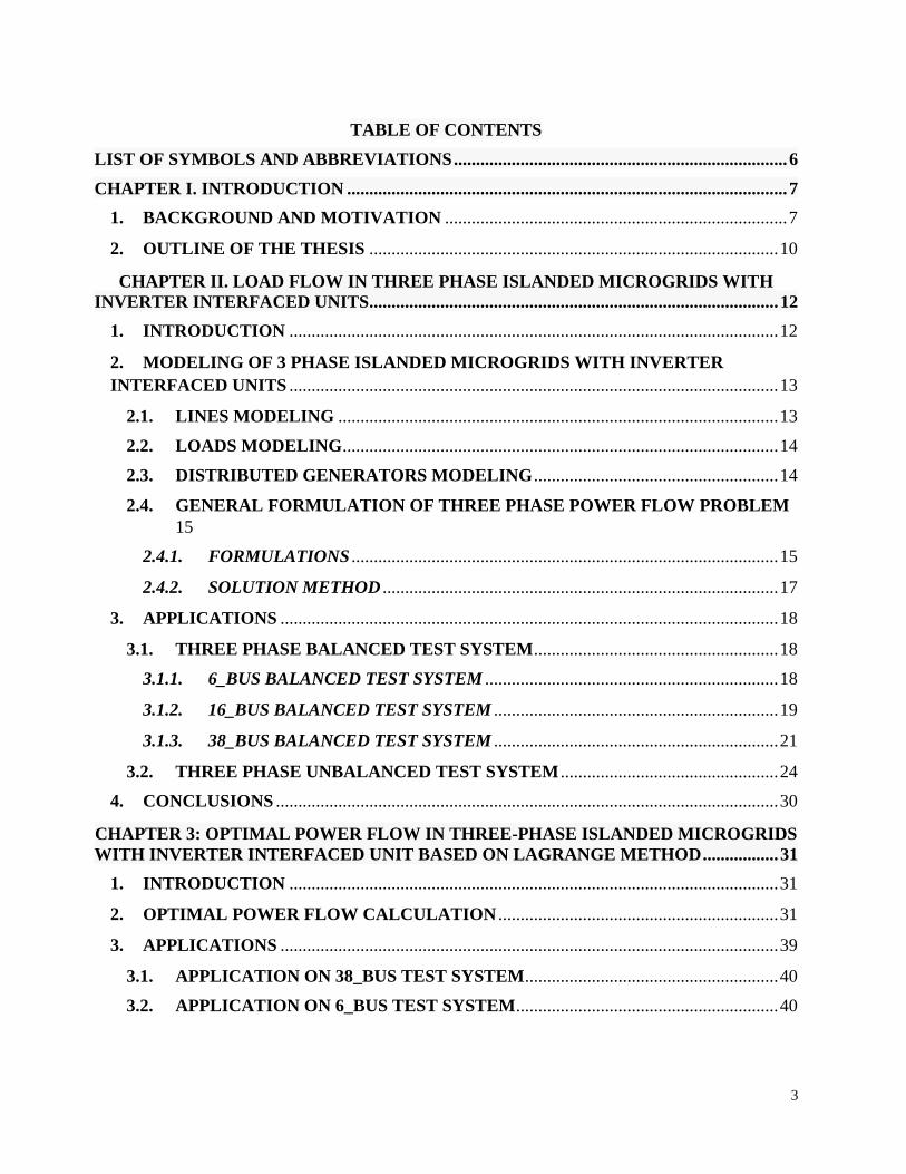
3.1.1. 6_BUS BALANCED TEST SYSTEM
Figure 4 shows the 6_bus balanced test system. As shown in the figure 4, three DG units
have been placed at buses 1, 2, and 3, respectively. The line-data and bus-data are shown in
Table I and Table II corresponding in I.1 Chapter 2 of appendix.
Figure 4 - 6_bus balanced test system
Voltage profile and loads results of the proposed power flow method on 6_bus
balanced system are shown in table I.

19
TABLE II. RESULT OF LOAD FLOW ON 6_BUS BALANCED SYSTEM, PU
Bus Vi di PGi Qgi PLi QLi
1 0.9871 0.0000 0.5825 0.3563 0.0000 0.0000
2 0.9793 -0.0075 0.4960 0.5724 0.0000 0.0000
3 0.9957 0.0303 0.7847 0.1177 0.0000 0.0000
4 0.9447 0.0061 0.0000 0.0000 0.7040 0.4017
5 0.9499 0.0062 0.0000 0.0000 0.3920 0.2026
6 0.9482 0.0166 0.0000 0.0000 0.6775 0.4021
Total PG QG PL QL f Ploss
1.8631 1.0465 1.7735 1.0064 0.9984 0.0896
Where Vi, di, PGi, Qgi, PLi, Qli are magnitude of voltage, voltage angle, generated real
power, generated reactive power, real power of load, reactive power of load at bus i respectively;
PG and QG are total generated real power, total generated reactive power, total real power of
loads, reactive power of loads in system respectively; f is frequency of system; Ploss is total real
power loss of system.
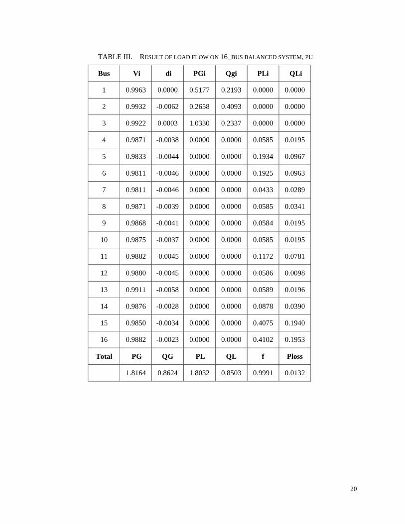
3.1.2. 16_BUS BALANCED TEST SYSTEM
Figure 5 shows the 16_bus balanced test system. In the figure 5, three DG units have been
placed at buses 1, 2, and 3, respectively. The line-data and bus-data are shown in Table III and
Table IV corresponding in I.1 Chapter 2 of appendix.
Voltage profile and loads results of the proposed power flow method on 16_bus balanced
system are shown in table II.
20
TABLE III. RESULT OF LOAD FLOW ON 16_BUS BALANCED SYSTEM, PU
Bus Vi di PGi Qgi PLi QLi
1 0.9963 0.0000 0.5177 0.2193 0.0000 0.0000
2 0.9932 -0.0062 0.2658 0.4093 0.0000 0.0000
3 0.9922 0.0003 1.0330 0.2337 0.0000 0.0000
4 0.9871 -0.0038 0.0000 0.0000 0.0585 0.0195
5 0.9833 -0.0044 0.0000 0.0000 0.1934 0.0967
6 0.9811 -0.0046 0.0000 0.0000 0.1925 0.0963
7 0.9811 -0.0046 0.0000 0.0000 0.0433 0.0289
8 0.9871 -0.0039 0.0000 0.0000 0.0585 0.0341
9 0.9868 -0.0041 0.0000 0.0000 0.0584 0.0195
10 0.9875 -0.0037 0.0000 0.0000 0.0585 0.0195
11 0.9882 -0.0045 0.0000 0.0000 0.1172 0.0781
12 0.9880 -0.0045 0.0000 0.0000 0.0586 0.0098
13 0.9911 -0.0058 0.0000 0.0000 0.0589 0.0196
14 0.9876 -0.0028 0.0000 0.0000 0.0878 0.0390
15 0.9850 -0.0034 0.0000 0.0000 0.4075 0.1940
16 0.9882 -0.0023 0.0000 0.0000 0.4102 0.1953
Total PG QG PL QL f Ploss
1.8164 0.8624 1.8032 0.8503 0.9991 0.0132

21
Figure 5 - 16_bus balanced test system
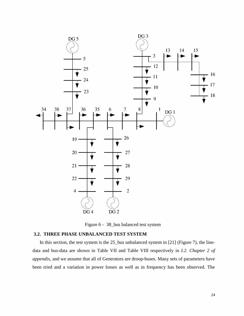
3.1.3. 38_BUS BALANCED TEST SYSTEM
Figure 6 shows the 38_bus balanced test system. In the figure 6, five DG units have been
placed at buses 1, 2, 3, 4 and 5 respectively. The line-data and bus-data are shown in Table V
and Table VI corresponding in I.1 Chapter 2 of appendix.
Voltage profile and loads results of the proposed power flow method on 38_bus balanced
system are shown in table III.
TABLE IV. RESULT OF LOAD FLOW ON 38_BUS BALANCED SYSTEM, PU
Bus Vi di PGi Qgi PLi QLi
1 1.0052 0.0000 1.0295 0.2875 0.0000 0.0000

22
Bus Vi di PGi Qgi PLi QLi
2 0.9945 -0.0011 0.7682 0.4663 0.0000 0.0000
3 0.9946 -0.0150 0.5592 0.4615 0.0000 0.0000
4 0.9955 -0.0108 0.5592 0.2901 0.0000 0.0000
5 0.9926 -0.0189 0.7682 0.6949 0.0000 0.0000
6 0.9831 -0.0148 0.0000 0.0000 0.0000 0.0000
7 0.9853 -0.0088 0.0000 0.0000 0.1951 0.0953
8 0.9889 -0.0093 0.0000 0.0000 0.1962 0.0965
9 0.9890 -0.0109 0.0000 0.0000 0.0597 0.0188
10 0.9895 -0.0123 0.0000 0.0000 0.0589 0.0193
11 0.9896 -0.0126 0.0000 0.0000 0.0442 0.0290
12 0.9899 -0.0131 0.0000 0.0000 0.0593 0.0337
13 0.9891 -0.0165 0.0000 0.0000 0.0589 0.0338
14 0.9871 -0.0177 0.0000 0.0000 0.1183 0.0761
15 0.9858 -0.0183 0.0000 0.0000 0.0586 0.0095
16 0.9846 -0.0186 0.0000 0.0000 0.0597 0.0183
17 0.9828 -0.0198 0.0000 0.0000 0.0583 0.0189
18 0.9822 -0.0200 0.0000 0.0000 0.0895 0.0360
19 0.9835 -0.0147 0.0000 0.0000 0.0884 0.0375
20 0.9877 -0.0139 0.0000 0.0000 0.0881 0.0384
21 0.9893 -0.0133 0.0000 0.0000 0.0896 0.0376
22 0.9928 -0.0116 0.0000 0.0000 0.0892 0.0390
23 0.9828 -0.0158 0.0000 0.0000 0.0874 0.0473
24 0.9838 -0.0178 0.0000 0.0000 0.4087 0.1897

23
Bus Vi di PGi Qgi PLi QLi
25 0.9880 -0.0191 0.0000 0.0000 0.4114 0.1925
26 0.9832 -0.0101 0.0000 0.0000 0.0583 0.0237
27 0.9827 -0.0094 0.0000 0.0000 0.0597 0.0226
28 0.9804 -0.0070 0.0000 0.0000 0.0581 0.0187
29 0.9790 -0.0050 0.0000 0.0000 0.1159 0.0653
30 0.9758 -0.0035 0.0000 0.0000 0.1922 0.5536
31 0.9721 -0.0049 0.0000 0.0000 0.1458 0.0626
32 0.9713 -0.0053 0.0000 0.0000 0.2039 0.0891
33 0.9711 -0.0054 0.0000 0.0000 0.0572 0.0363
34 0.9837 -0.0105 0.0000 0.0000 0.0597 0.0182
35 0.9831 -0.0148 0.0000 0.0000 0.0982 0.0562
36 0.9827 -0.0147 0.0000 0.0000 0.0895 0.0361
37 0.9826 -0.0139 0.0000 0.0000 0.1166 0.0756
38 0.9830 -0.0130 0.0000 0.0000 0.0589 0.0281
Total PG QG PL QL f Ploss
3.6844 2.2003 3.6332 2.1532 0.9974 0.0512
24
Figure 6 - 38_bus balanced test system
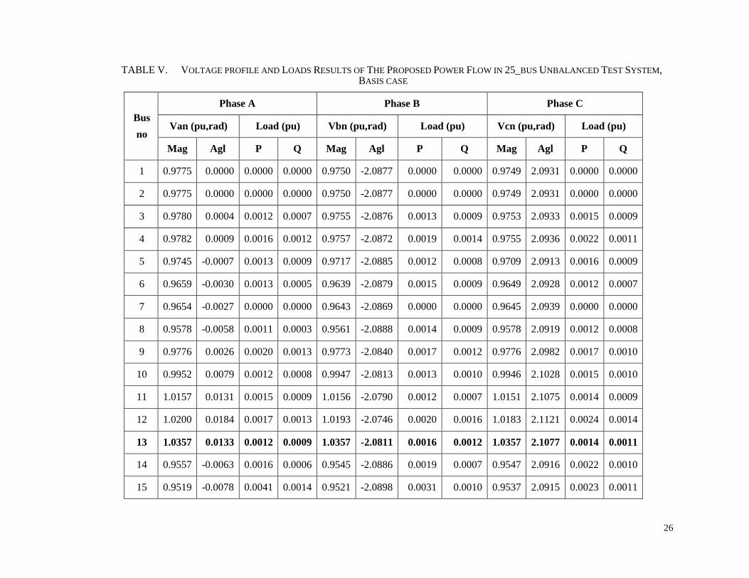
3.2. THREE PHASE UNBALANCED TEST SYSTEM
In this section, the test system is the 25_bus unbalanced system in [21] (Figure 7), the line-
data and bus-data are shown in Table VII and Table VIII respectively in I.2. Chapter 2 of
appendix, and we assume that all of Generators are droop-buses. Many sets of parameters have
been tried and a variation in power losses as well as in frequency has been observed. The

25
following underlying hypotheses have been made: the base power and base voltage for per unit
calculations have been set to SB = 30MVA, VB = 4.16 kV.
Using the proposed method we get the power load flow results (voltage profile and loads in
each phase; the real and reactive power in each phase and the total injected power from all the
DG units in p.u) are shown in table IV and V respectively.
Figure 7 - 25_bus unbalanced test system
26
TABLE V. VOLTAGE PROFILE AND LOADS RESULTS OF THE PROPOSED POWER FLOW IN 25_BUS UNBALANCED TEST SYSTEM, BASIS CASE
Bus
no
Phase A Phase B Phase C
Van (pu,rad) Load (pu) Vbn (pu,rad) Load (pu) Vcn (pu,rad) Load (pu)
Mag Agl P Q Mag Agl P Q Mag Agl P Q
1 0.9775 0.0000 0.0000 0.0000 0.9750 -2.0877 0.0000 0.0000 0.9749 2.0931 0.0000 0.0000
2 0.9775 0.0000 0.0000 0.0000 0.9750 -2.0877 0.0000 0.0000 0.9749 2.0931 0.0000 0.0000
3 0.9780 0.0004 0.0012 0.0007 0.9755 -2.0876 0.0013 0.0009 0.9753 2.0933 0.0015 0.0009
4 0.9782 0.0009 0.0016 0.0012 0.9757 -2.0872 0.0019 0.0014 0.9755 2.0936 0.0022 0.0011
5 0.9745 -0.0007 0.0013 0.0009 0.9717 -2.0885 0.0012 0.0008 0.9709 2.0913 0.0016 0.0009
6 0.9659 -0.0030 0.0013 0.0005 0.9639 -2.0879 0.0015 0.0009 0.9649 2.0928 0.0012 0.0007
7 0.9654 -0.0027 0.0000 0.0000 0.9643 -2.0869 0.0000 0.0000 0.9645 2.0939 0.0000 0.0000
8 0.9578 -0.0058 0.0011 0.0003 0.9561 -2.0888 0.0014 0.0009 0.9578 2.0919 0.0012 0.0008
9 0.9776 0.0026 0.0020 0.0013 0.9773 -2.0840 0.0017 0.0012 0.9776 2.0982 0.0017 0.0010
10 0.9952 0.0079 0.0012 0.0008 0.9947 -2.0813 0.0013 0.0010 0.9946 2.1028 0.0015 0.0010
11 1.0157 0.0131 0.0015 0.0009 1.0156 -2.0790 0.0012 0.0007 1.0151 2.1075 0.0014 0.0009
12 1.0200 0.0184 0.0017 0.0013 1.0193 -2.0746 0.0020 0.0016 1.0183 2.1121 0.0024 0.0014
13 1.0357 0.0133 0.0012 0.0009 1.0357 -2.0811 0.0016 0.0012 1.0357 2.1077 0.0014 0.0011
14 0.9557 -0.0063 0.0016 0.0006 0.9545 -2.0886 0.0019 0.0007 0.9547 2.0916 0.0022 0.0010
15 0.9519 -0.0078 0.0041 0.0014 0.9521 -2.0898 0.0031 0.0010 0.9537 2.0915 0.0023 0.0011
27
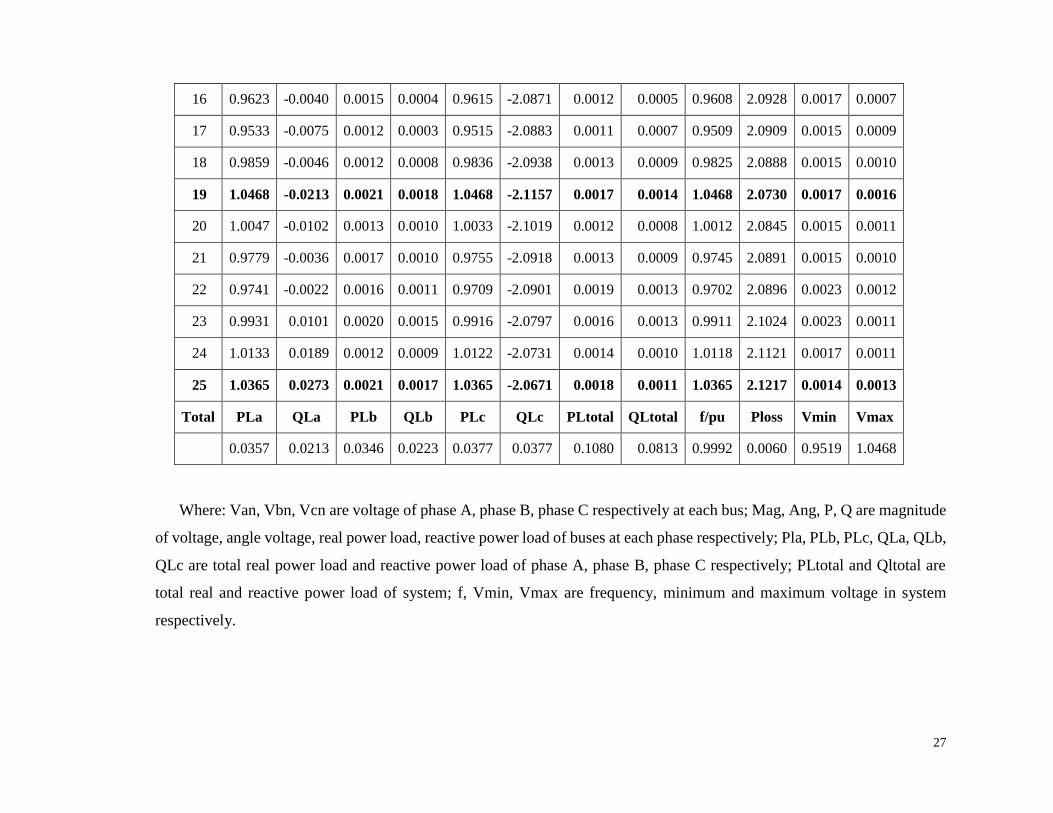
16 0.9623 -0.0040 0.0015 0.0004 0.9615 -2.0871 0.0012 0.0005 0.9608 2.0928 0.0017 0.0007
17 0.9533 -0.0075 0.0012 0.0003 0.9515 -2.0883 0.0011 0.0007 0.9509 2.0909 0.0015 0.0009
18 0.9859 -0.0046 0.0012 0.0008 0.9836 -2.0938 0.0013 0.0009 0.9825 2.0888 0.0015 0.0010
19 1.0468 -0.0213 0.0021 0.0018 1.0468 -2.1157 0.0017 0.0014 1.0468 2.0730 0.0017 0.0016
20 1.0047 -0.0102 0.0013 0.0010 1.0033 -2.1019 0.0012 0.0008 1.0012 2.0845 0.0015 0.0011
21 0.9779 -0.0036 0.0017 0.0010 0.9755 -2.0918 0.0013 0.0009 0.9745 2.0891 0.0015 0.0010
22 0.9741 -0.0022 0.0016 0.0011 0.9709 -2.0901 0.0019 0.0013 0.9702 2.0896 0.0023 0.0012
23 0.9931 0.0101 0.0020 0.0015 0.9916 -2.0797 0.0016 0.0013 0.9911 2.1024 0.0023 0.0011
24 1.0133 0.0189 0.0012 0.0009 1.0122 -2.0731 0.0014 0.0010 1.0118 2.1121 0.0017 0.0011
25 1.0365 0.0273 0.0021 0.0017 1.0365 -2.0671 0.0018 0.0011 1.0365 2.1217 0.0014 0.0013
Total PLa QLa PLb QLb PLc QLc PLtotal QLtotal f/pu Ploss Vmin Vmax
0.0357 0.0213 0.0346 0.0223 0.0377 0.0377 0.1080 0.0813 0.9992 0.0060 0.9519 1.0468
Where: Van, Vbn, Vcn are voltage of phase A, phase B, phase C respectively at each bus; Mag, Ang, P, Q are magnitude
of voltage, angle voltage, real power load, reactive power load of buses at each phase respectively; Pla, PLb, PLc, QLa, QLb,
QLc are total real power load and reactive power load of phase A, phase B, phase C respectively; PLtotal and Qltotal are
total real and reactive power load of system; f, Vmin, Vmax are frequency, minimum and maximum voltage in system
respectively.

28
TABLE VI. DG UNITS REAL AND REACTIVE POWER GENERATION IN 25_BUS UNBALANCED TEST
SYSTEM
Bus
ID of Gen 𝐏𝐆𝐚 𝐏𝐆𝐛 𝐏𝐆𝐜 𝐐𝐆𝐚 𝐐𝐆𝐛 𝐐𝐆𝐜
𝐏𝐆
total
𝐐𝐆
total
13 0.0092 0.0094 0.0099 0.0066 0.0072 0.0078 0.0285 0.0217
19 0.0096 0.0091 0.0098 0.0104 0.0107 0.0108 0.0285 0.0320
25 0.0188 0.0182 0.0200 0.0056 0.0057 0.0060 0.0570 0.0173
Where: PGa, PGb, PGc, QGa, QGb, QGc are real and reactive generated power at each phase of
each generator respectively; PGtotal and QGtotal are total real and reactive generated power of
each generator.
Taking the values reported in Table VI for parameters 𝐾𝐺𝑖 , 𝐾𝑑𝑖, 𝑉0𝑖, 𝑓0𝑖 for the inverter
interfaced generators, the following results for frequency and power losses are obtained. In all
the results reported voltage drops in all buses are below the admissible values (5%).
TABLE VII. GENERAL RESULT
Bus
ID of Gen 𝐊𝐝𝐢
𝐕𝟎𝐢
/pu 𝐊𝐆𝐢 𝐟𝟎𝐢/pu 𝐟 /pu
Ploss
/pu
Vmin
/pu
Vmax
/pu
13 5.00 1.0400 10.00 1.0020
0.9992 0.0060 0.9519 1.0468 19 10.00 1.0500 10.00 1.0020
25 5.00 1.0400 20.00 1.0020
Change the value of 𝐾𝐺 , 𝐾𝑑, 𝑉0 and 𝑓0 of generators and calculating the power flows, we get
the first results that are shown in Tables VII to XI. In all the trials, the parameters that stay
unchanged (𝐾𝐺𝑖 , 𝐾𝑑𝑖, 𝑉0𝑖, 𝑓0𝑖) assume the values in Table IV. In table VI, only parameter KG13
has been changed.

29
TABLE VIII. LOSSES AND FREQUENCY IN THE TEST SYSTEM, CHANGING KG13
𝐊𝐆𝟏𝟑 f/pu Ploss/pu Vmin/pu Vmax/pu
30.00 1.0000 0.0101 0.9502 1.0454
20.00 0.9997 0.0075 0.9513 1.0460
10.00 0.9992 0.0060 0.9519 1.0468
TABLE IX. LOSSES AND FREQUENCY IN THE TEST SYSTEM, CHANGING KG25
𝐊𝐆𝟐𝟓 f/pu Ploss/pu Vmin/pu Vmax/pu
40.00 1.0000 0.0090 0.9518 1.0455
30.00 0.9997 0.0074 0.9520 1.0460
20.00 0.9992 0.0060 0.9519 1.0468
TABLE X. LOSSES AND FREQUENCY IN THE TEST SYSTEM, CHANGING KG13 AND KG19
KG13 KG19 f/pu Ploss/pu Vmin/pu Vmax/pu
10.00 10.00 0.9992 0.0060 0.9519 1.0468
15.00 15.00 0.9997 0.0055 0.9516 1.0475
15.00 20.00 0.9999 0.0058 0.9509 1.0484
17.00 20.00 1.0000 0.0057 0.9510 1.0482
TABLE XI. LOSSES AND FREQUENCY IN THE TEST SYSTEM, CHANGING KG13 AND F025
KG13 f025 f/pu Ploss/pu Vmin/pu Vmax/pu
10.00 1.0020 0.9992 0.0060 0.9519 1.0468
10.00 1.0030 0.9996 0.0072 0.952 1.0462
18.00 1.0030 1.0000 0.0079 0.9516 1.0455
10.00 1.0035 0.9998 0.0080 0.9519 1.0458
13.00 1.0035 1.0000 0.0082 0.9518 1.0456

30
TABLE XII. LOSSES AND FREQUENCY IN THE TEST SYSTEM, CHANGING KG19 AND F025
KG19 f025 f/pu Ploss/pu Vmin/pu Vmax/pu
10.00 1.0020 0.9992 0.0060 0.9519 1.0468
15.00 1.0030 0.9999 0.0061 0.9518 1.0472
17.00 1.0030 1.0000 0.0060 0.9517 1.0476
15.00 1.0031 0.9999 0.0062 0.9519 1.0471
15.00 1.0032 1.0000 0.0063 0.9519 1.0471
In the tables, in italic, the parameters of basic case taking value from table VI, while in bold
are evidenced the sets of parameters showing the rated frequency value. As it can be observed,
there are many different sets of parameters (marked in bold in each table) satisfying the condition
f = 50Hz, in all cases, however, the frequency does not vary for more than 0.2 Hz as prescribed
by the IEEE standard while power losses change. So it means that changing system parameters
will produce a change of the power loss in the system. With f within the admissible range, the
set of parameters satisfying the condition of minimum power losses can thus be chosen for
optimal system operation.
4. CONCLUSIONS
This chapter proposes the use of the Trust Region Method to solve the power flow problem
in 3 phase balanced and unbalanced microgrid system. Authors have applied the proposed
method on many kind of test system in both balanced and unbalanced mode. In the 25_test bus
unbalanced system, the results shows how the power losses term varies as the regulators
parameters vary as well, thus showing that these are sensitive parameters that could have an
important role in optimal management of such systems. These results suggest an idea for further
work on optimal system operation considering also stability issues.

31
CHAPTER 3: OPTIMAL POWER FLOW IN THREE-PHASE
ISLANDED MICROGRIDS WITH INVERTER INTERFACED
UNIT BASED ON LAGRANGE METHOD
1. INTRODUCTION
In this chapter, the solution of the OPF problem for three phase islanded microgrids is
studied, the OPF being one of the core functions of the tertiary regulation level for an AC
islanded microgrid with a hierarchical control architecture. The study also aims at evaluating the
contextual adjustment of the droop parameters used for primary voltage and frequency
regulation of inverter interfaced units. The work proposes a mathematical method for the OPF
solution also considering the droop parameters as variables. The output of the OPF provides an
iso-frequential operating point for all the generation units and a set of droop parameters for
primary regulation. In this way, secondary regulation can be neglected in the considered
hierarchical control structure. Finally, the application section provides the solution of the OPF
problem over networks of different sizes and a stability analysis of the microgrid system using
the optimized droop parameters, thus giving rise to the optimized management of the system
with a new hierarchical control architecture.
2. OPTIMAL POWER FLOW CALCULATION
The OPF in this paper is carried out to minimize power losses. The solution algorithm is
iterative and uses Lagrange method. The solution strategy has proved to be efficient for the
definition of new operating points and new droop parameters for primary regulation; moreover,
the proposed architecture integrating the proposed OPF may replace the secondary regulation
level by finding an iso-frequency working condition for all units. It has indeed been shown,
through parametric studies, in Chapter 2, that the power losses term is of course connected to
the droop parameters values and thus such choice influences the steady state operation of
microgrids.
Moreover sharing power among units so as to get a minimum loss operation will lead also
to increased stability margins and probably a stable operation as proved in [22], [23].
32
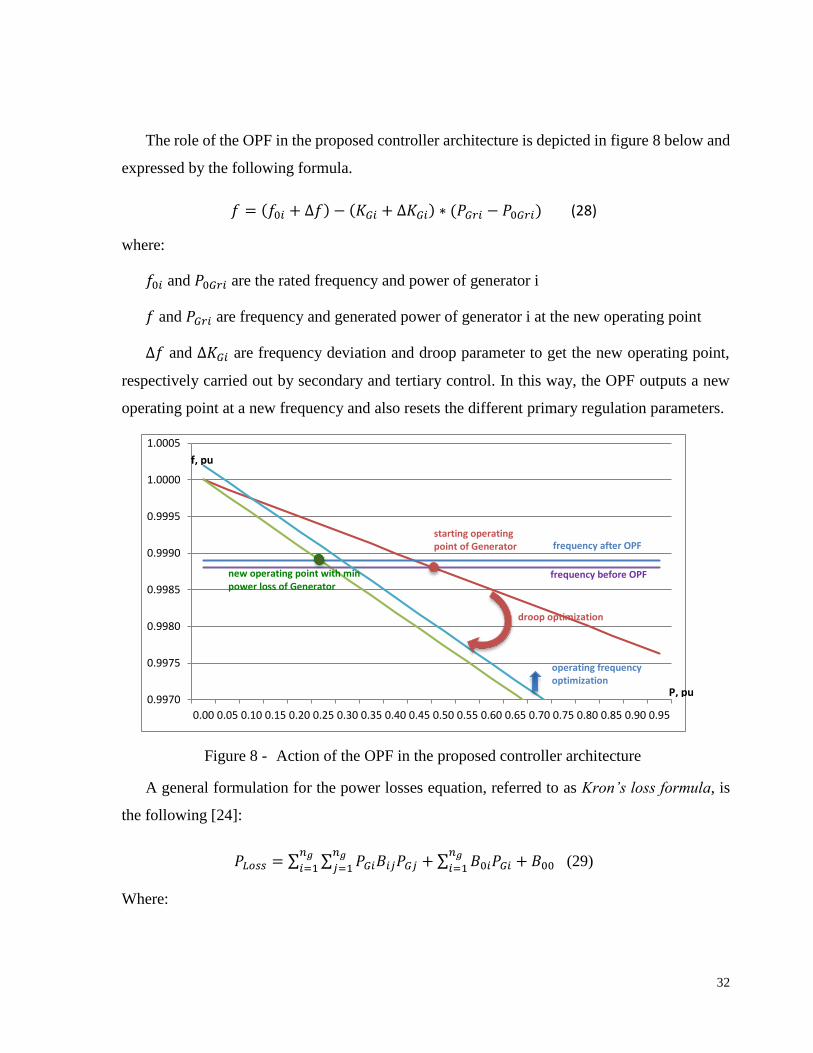
The role of the OPF in the proposed controller architecture is depicted in figure 8 below and
expressed by the following formula.
𝑓 = (𝑓0𝑖 + ∆𝑓) − (𝐾𝐺𝑖 + ∆𝐾𝐺𝑖) ∗ (𝑃𝐺𝑟𝑖 − 𝑃0𝐺𝑟𝑖) (28)
where:
𝑓0𝑖 and 𝑃0𝐺𝑟𝑖 are the rated frequency and power of generator i
𝑓 and 𝑃𝐺𝑟𝑖 are frequency and generated power of generator i at the new operating point
∆𝑓 and ∆𝐾𝐺𝑖 are frequency deviation and droop parameter to get the new operating point,
respectively carried out by secondary and tertiary control. In this way, the OPF outputs a new
operating point at a new frequency and also resets the different primary regulation parameters.
Figure 8 - Action of the OPF in the proposed controller architecture
A general formulation for the power losses equation, referred to as Kron’s loss formula, is
the following [24]:
𝑃𝐿𝑜𝑠𝑠 = ∑ ∑ 𝑃𝐺𝑖𝐵𝑖𝑗𝑃𝐺𝑗 + ∑ 𝐵0𝑖𝑃𝐺𝑖𝑛𝑔𝑖=1
+ 𝐵00𝑛𝑔𝑗=1
𝑛𝑔𝑖=1
(29)
Where:
0.9970
0.9975
0.9980
0.9985
0.9990
0.9995
1.0000
1.0005
0.00 0.05 0.10 0.15 0.20 0.25 0.30 0.35 0.40 0.45 0.50 0.55 0.60 0.65 0.70 0.75 0.80 0.85 0.90 0.95
starting operating point of Generator
new operating point with min power loss of Generator
frequency before OPF
frequency after OPF
droop optimization
operating frequency optimization
P, pu
f, pu

33
𝑛𝑔 is the number of generators (including of droop generators ( 𝑛𝑔𝑟) and PQ generators
(𝑛𝑃𝑄)),
𝑃𝐺𝑖 and 𝑃𝐺𝑗 are matrix of generated real powers
𝑃𝐺𝑗 = [
𝑃𝐺1𝑃𝐺2⋮
𝑃𝐺𝑛𝑔
]; 𝑃𝐺𝑖 = [𝑃𝐺1 𝑃𝐺2 … 𝑃𝐺𝑛𝑔] (30)
𝐵𝑖𝑗, 𝐵0𝑖 and 𝐵00are loss coefficients or B-coefficients.
Such formulation linearly relates the power losses with the generated powers, considering
constant the system’s frequency and bus voltages modules and displacements. Although the
expression was originally written for transmission systems, it can also be used for microgrids,
since it does not imply any assumption that is strictly valid for transmission. Besides, in the
solution algorithm, the B-coefficients formulation for power losses is re-calculated at each
iteration and this will be cleared out in later. The algorithm repeatedly calculates the system’s
electrical parameters (voltages modules, voltages displacements and frequency) through the
solution of the power flow for new values of the generated power. Nonetheless, since the B-
coefficient formulation is adequate for systems that have balanced loads, this hypothesis is a
basic assumption to use the proposed method.
The three phase injected real and reactive power from a DG unit which is Droop_bus are
calculated in (4) and (5) and in this application, the reactive power depends on voltage but the
relevant parameter (𝐾𝑑𝑖) can not be optimized.
The optimal dispatch problem is thus that to find the set of droop parameters (𝐾𝐺𝑖) and
generating powers (𝑃𝐺𝑖) minimizing the power losses function expressed in (27), subject to the
constraint that generation should equal total demands plus losses
∑ 𝑃𝐺𝑟𝑖 + ∑ 𝑃𝑃𝑄𝑖𝑛𝑃𝑄𝑖=1
= ∑ 𝑃𝐿𝑖𝑛𝑑𝑖=1 + 𝑃𝐿𝑜𝑠𝑠
𝑛𝑔𝑟𝑖=1
(31)
where 𝑃𝐺𝑟𝑖 is the real power of droop_generator i; 𝑃𝑃𝑄𝑖 is the real power of PQ_generator i; 𝑃𝐿𝑖
is the real power of load bus i and 𝑛𝑑 is the number of load bus.

34
The problem should also meet the following inequality constraints, expressed as follows:
𝐾𝐺𝑖𝑚𝑖𝑛 ≤ 𝐾𝐺𝑖 ≤ 𝐾𝐺𝑖𝑚𝑎𝑥 , 𝑖 = 1 to 𝑛𝑔𝑟 (32)
𝑃𝑃𝑄𝑖𝑚𝑖𝑛 ≤ 𝑃𝑃𝑄𝑖 ≤ 𝑃𝑃𝑄𝑖𝑚𝑎𝑥 , 𝑖 = 1 to 𝑛𝑃𝑄 (33)
where the KGi is a coefficient characterizing the droop regulator of droop_bus generator i, 𝐼𝑚𝑛𝑖
is the current on branch mn connecting buses m and n.
Following the Lagrange method, we obtain
𝐿 = 𝑃𝐿𝑜𝑠𝑠 + 𝜆(∑ 𝑃𝐿𝑖𝑛𝑑𝑖=1 + 𝑃𝐿𝑜𝑠𝑠 − ∑ 𝑃𝐺𝑟𝑖 − ∑ 𝑃𝑃𝑄𝑖
𝑛𝑃𝑄𝑖=1
𝑛𝑔𝑟𝑖=1
) +
∑ 𝜇𝑖(𝑚𝑎𝑥)(𝐾𝐺𝑖 − 𝐾𝐺𝑖(𝑚𝑎𝑥))𝑛𝑔𝑟𝑖=1
+∑ 𝜇𝑖(𝑚𝑖𝑛)(𝐾𝐺𝑖 − 𝐾𝐺𝑖(𝑚𝑖𝑛)) + ∑ 𝛾𝑖(𝑚𝑎𝑥)(𝑃𝑃𝑄𝑖 −𝑛𝑃𝑄𝑖=1
𝑛𝑔𝑟𝑖=1
𝑃𝑃𝑄𝑖𝑚𝑎𝑥) +∑ 𝛾𝑖(𝑚𝑖𝑛)(𝑃𝑃𝑄𝑖 − 𝑃𝑃𝑄𝑖𝑚𝑖𝑛)𝑛𝑃𝑄𝑖=1
(34)
where 𝜆, 𝜇𝑖(𝑚𝑎𝑥), 𝜇𝑖(𝑚𝑖𝑛), 𝛾𝑖(𝑚𝑎𝑥), 𝛾𝑖(𝑚𝑖𝑛) are the Lagrange multiplier and the 𝜇𝑖(𝑚𝑎𝑥) =
0, 𝛾𝑖(𝑚𝑎𝑥) = 0 when 𝐾𝐺𝑖 < 𝐾𝐺𝑖𝑚𝑎𝑥, 𝑃𝑃𝑄𝑖 < 𝑃𝑃𝑄𝑖𝑚𝑎𝑥 ; 𝜇𝑖(𝑚𝑖𝑛) = 0, 𝛾𝑖(𝑚𝑖𝑛) = 0 when 𝐾𝐺𝑖 >
𝐾𝐺𝑖𝑚𝑖𝑛, 𝑃𝑃𝑄𝑖 > 𝑃𝑃𝑄𝑖𝑚𝑖𝑛. It means that if the constraint is violated, it will become active. To get
the solution of the problem, we have to solve the set of equations include of the partials of the
function below:
𝜕𝐿
𝜕𝐾𝐺𝑖= 0 (35)
𝜕𝐿
𝜕𝑃𝑃𝑄𝑖= 0 (36)
𝜕𝐿
𝜕𝜆= 0 (37)
𝜕𝐿
𝜕𝜇𝑚𝑎𝑥= 𝐾𝐺𝑖 − 𝐾𝐺𝑖(𝑚𝑎𝑥) = 0 (38)
𝜕𝐿
𝜕𝜇𝑚𝑖𝑛= 𝐾𝐺𝑖 − 𝐾𝐺𝑖(𝑚𝑖𝑛) = 0 (39)
𝜕𝐿
𝜕𝛾𝑚𝑎𝑥= 𝑃𝑃𝑄𝑖 − 𝑃𝑃𝑄𝑖(𝑚𝑎𝑥) = 0 (40)
𝜕𝐿
𝜕𝛾𝑚𝑖𝑛= 𝑃𝑃𝑄𝑖 − 𝑃𝑃𝑄𝑖(𝑚𝑖𝑛) = 0 (41)
35
Equations (38), (39), (40) and (41) mean that when 𝐾𝐺𝑖 and 𝑃𝑃𝑄𝑖 are within their limits, we
will have:
𝜇𝑖(𝑚𝑖𝑛) = 𝜇𝑖(𝑚𝑎𝑥) = 0 (42)
and
𝛾𝑖(𝑚𝑖𝑛) = 𝛾𝑖(𝑚𝑎𝑥) = 0 (43)
First condition, given by (35) results in
𝜕𝐿
𝜕𝐾𝐺𝑖=
𝜕𝑃𝐿𝑜𝑠𝑠
𝜕𝐾𝐺𝑖+ 𝜆 (
𝜕∑ 𝑃𝐿𝑖𝑛𝑑𝑖=1
𝜕𝐾𝐺𝑖+𝜕𝑃𝐿𝑜𝑠𝑠
𝜕𝐾𝐺𝑖−𝜕 ∑ 𝑃𝐺𝑟𝑖
𝑛𝑔𝑟𝑖=1
𝜕𝐾𝐺𝑖−𝜕∑ 𝑃𝑃𝑄𝑖
𝑛𝑃𝑄𝑖=1
𝜕𝐾𝐺𝑖) = 0 (44)
Since
𝜕∑ 𝑃𝐺𝑟𝑖𝑛𝑔𝑟𝑖=1
𝜕𝐾𝐺𝑖=
𝑑𝑃𝐺𝑟𝑖
𝑑𝐾𝐺𝑖= −(𝑓 − 𝑓0𝑖) (45)
𝜕∑ 𝑃𝑃𝑄𝑖𝑛𝑃𝑄𝑖=1
𝜕𝐾𝐺𝑖= 0 (46)
𝜕∑ 𝑃𝐿𝑖𝑛𝑑𝑖=1
𝜕𝐾𝐺𝑖=
𝑑𝑃𝐿𝑖
𝑑𝐾𝐺𝑖= 0 (47)
And therefore the condition for optimum dispatch becomes
𝜕𝑃𝐿𝑜𝑠𝑠
𝜕𝐾𝐺𝑖(𝜆 + 1) + 𝜆(𝑓 − 𝑓0𝑖) = 0 (48)
Since
𝜕𝑃𝐿𝑜𝑠𝑠
𝜕𝐾𝐺𝑖= (𝑓 − 𝑓0𝑖) (−2∑ 𝐵𝑖𝑗𝑃𝐺𝑗
𝑛𝑔𝑗=1
− 𝐵0𝑖) (49)
substituting in (48) we have
2∑ 𝐵𝑖𝑗𝑃𝐺𝑗𝑛𝑔𝑗=1
+ 𝐵0𝑖 (𝜆 + 1) − 𝜆 = 0 (50)
or

36
𝐵𝑖𝑖(𝑓 − 𝑓𝑜𝑖)𝐾𝐺𝑖 − ∑ 𝐵𝑖𝑗𝑃𝐺𝑗 =𝐵0𝑖
2
𝑛𝑔𝑗=1𝑗≠𝑖
−𝜆
2(𝜆+1) (51)
Second condition, given by (36) results in
𝜕𝐿
𝜕𝑃𝑃𝑄𝑖=
𝜕𝑃𝐿𝑜𝑠𝑠
𝜕𝑃𝑃𝑄𝑖+ 𝜆 (
𝜕∑ 𝑃𝐿𝑖𝑛𝑑𝑖=1
𝜕𝑃𝑃𝑄𝑖+𝜕𝑃𝐿𝑜𝑠𝑠
𝜕𝑃𝑃𝑄𝑖−𝜕∑ 𝑃𝐺𝑟𝑖
𝑛𝑔𝑟𝑖=1
𝜕𝑃𝑃𝑄𝑖−𝜕∑ 𝑃𝑃𝑄𝑖
𝑛𝑃𝑄𝑖=1
𝜕𝑃𝑃𝑄𝑖) = 0 (52)
Since
𝜕∑ 𝑃𝐺𝑟𝑖𝑛𝑔𝑟𝑖=1
𝜕𝑃𝑃𝑄𝑖= 0 (53)
𝜕∑ 𝑃𝑃𝑄𝑖𝑛𝑃𝑄𝑖=1
𝜕𝑃𝑃𝑄𝑖= 1 (54)
𝜕∑ 𝑃𝐿𝑖𝑛𝑑𝑖=1
𝜕𝑃𝑃𝑄𝑖=
𝑑𝑃𝐿𝑖
𝑑𝑃𝑃𝑄𝑖= 0 (55)
And therefore the condition for optimum dispatch becomes
𝜕𝑃𝐿𝑜𝑠𝑠
𝜕𝑃𝑃𝑄𝑖(𝜆 + 1) − 𝜆 = 0 (56)
Since
𝜕𝑃𝐿𝑜𝑠𝑠
𝜕𝑃𝑃𝑄𝑖= 2∑ 𝐵𝑖𝑗𝑃𝐺𝑗
𝑛𝑔𝑗=1
+ 𝐵0𝑖 (57)
substituting in (56) we have
2∑ 𝐵𝑖𝑗𝑃𝐺𝑗𝑛𝑔𝑗=1
+ 𝐵0𝑖 (𝜆 + 1) − 𝜆 = 0 (58)
or
𝐵𝑖𝑖𝑃𝑃𝑄𝑖 + ∑ 𝐵𝑖𝑗𝑃𝐺𝑗 =𝜆
2(𝜆+1)−𝐵0𝑖
2
𝑛𝑔𝑗=1𝑗≠𝑖
(59)
Third condition, given by (37) results in
∑ 𝑃𝐿𝑖𝑛𝑑𝑖=1 + 𝑃𝐿𝑜𝑠𝑠 − ∑ 𝑃𝐺𝑟𝑖 −∑ 𝑃𝑃𝑄𝑖
𝑛𝑃𝑄𝑖=1
𝑛𝑔𝑟𝑖=1
= 0 (60)
37
Expressing (51) and (59) in form of matrix, we have
[ 𝐵11 𝐵12 … 𝐵1𝑛𝑔𝐵21⋮
𝐵𝑛𝑔1
𝐵22⋮
𝐵𝑛𝑔2
…⋱…
𝐵2𝑛𝑔⋮
𝐵𝑛𝑔𝑛𝑔]
[ 𝐾𝐺1(𝑓 − 𝑓01)
𝐾𝐺2(𝑓 − 𝑓02)⋮
−𝑃𝑃𝑄1⋮
𝐾𝐺𝑛𝑔(𝑓 − 𝑓0𝑛𝑔)]
=1
2
[ 𝐵01 −
𝜆
𝜆+1
𝐵02 −𝜆
𝜆+1
⋮
𝐵0𝑛𝑔 −𝜆
𝜆+1]
(61)
We use the gradient method to solve this set of equation in (61). First, we estimated an initial
value of 𝜆(𝑘), then we can solve the set of linear equations. From (61), formulation to calculate
𝐾𝐺𝑖 at the 𝑘𝑡ℎ iteration can be extracted as
𝐾𝐺𝑖(𝑘) =
𝐵𝑜𝑖(𝜆(𝑘)+1)−𝜆(𝑘)−2(𝜆(𝑘)+1)∑ 𝐵𝑖𝑗𝐾𝐺𝑗
(𝑘)(𝑓−𝑓0𝑗)𝑛𝑔𝑗=1𝑗≠𝑖
2(𝜆(𝑘)+1)𝐵𝑖𝑖(𝑓−𝑓0𝑖) (62)
From (61), formulation to calculate 𝑃𝑃𝑄𝑖 at the 𝑘𝑡ℎ iteration can be extracted as
𝑃𝑃𝑄𝑖(𝑘) =
−𝐵𝑜𝑖(𝜆(𝑘)+1)+𝜆(𝑘)−2(𝜆(𝑘)+1)∑ 𝐵𝑖𝑗𝑃𝐺𝑗
(𝑘)𝑛𝑔𝑗=1𝑗≠𝑖
2(𝜆(𝑘)+1)𝐵𝑖𝑖 (63)
Substituting for 𝐾𝐺𝑖 from (62) in (5) to get 𝑃𝐺𝑟𝑖 and then substituting 𝑃𝑃𝑄𝑖 from (63) and 𝑃𝐺𝑟𝑖
in (60) we have
−∑
𝐵𝑜𝑖(𝜆(𝑘)+1)−𝜆(𝑘)−2(𝜆(𝑘)+1)∑ 𝐵𝑖𝑗𝐾𝐺𝑗
(𝑘)(𝑓−𝑓0𝑗)𝑛𝑔𝑗=1𝑗≠𝑖
2(𝜆(𝑘)+1)𝐵𝑖𝑖
𝑛𝑔𝑟𝑖=1 +
∑
−𝐵𝑜𝑖(𝜆(𝑘)+1)+𝜆(𝑘)−2(𝜆(𝑘)+1)∑ 𝐵𝑖𝑗𝑃𝐺𝑗
(𝑘)𝑛𝑔𝑗=1𝑗≠𝑖
2(𝜆(𝑘)+1)𝐵𝑖𝑖
𝑛𝑃𝑄𝑖=1 = ∑ 𝑃𝐿𝑖
𝑛𝑑𝑖=1 + 𝑃𝐿𝑜𝑠𝑠
(k) (64)
or
∑
−𝐵𝑜𝑖(𝜆(𝑘)+1)+𝜆(𝑘)−2(𝜆(𝑘)+1)∑ 𝐵𝑖𝑗𝑃𝐺𝑗
(𝑘)𝑛𝑔𝑗=1𝑗≠𝑖
2(𝜆(𝑘)+1)𝐵𝑖𝑖
𝑛𝑔𝑖=1 = ∑ 𝑃𝐿𝑖
𝑛𝑑𝑖=1 + 𝑃𝐿𝑜𝑠𝑠
(k) (65)
or
𝑔(𝜆(𝑘)) = ∑ 𝑃𝐿𝑖𝑛𝑑𝑖=1 + 𝑃𝐿𝑜𝑠𝑠
(k) (66)
38
Expanding 𝑔(𝜆(𝑘)) in Taylor’s series about an operating point 𝜆(𝑘), and neglecting the
higher-order terms we get
𝑔(𝜆(𝑘)) + (𝑑𝑔(𝜆)
𝑑𝜆)(𝑘)
Δ𝜆(𝑘) = ∑ 𝑃𝐿𝑖𝑛𝑑𝑖=1 + 𝑃𝐿𝑜𝑠𝑠
(k) (67)
or
Δ𝜆(𝑘) =∑ 𝑃𝐿𝑖𝑛𝑑𝑖=1
+𝑃𝐿𝑜𝑠𝑠 (k)−𝑔(𝜆(𝑘))
(𝑑𝑔(𝜆)
𝑑𝜆)(𝑘) =
Δ𝑃(𝑘)
∑(𝑑𝑃𝑖𝑑𝜆)(𝑘) (68)
where
∑ (𝑑𝑃𝑖
𝑑𝜆)(𝑘)
= ∑1
2(𝜆(𝑘)+1)2𝐵𝑖𝑖
𝑛𝑔𝑖=1
𝑛𝑔𝑖=1 (69)
and therefore
𝜆(𝑘+1) = 𝜆(𝑘) + Δ𝜆(𝑘) (70)
The flowchart of the algorithm is shown in figure 9. To get the solution, first we give an
initial value in range of variables: Kg0 and PPQ0, set the accuracy 휀 and the first value of deviation
of real generated power ∆𝑃𝑔0 and ∆𝑃𝑃𝑄0 satisfying ∆𝑃𝑔0 < 휀 & ∆𝑃𝑃𝑄
0 < 휀. Next we use
proposed method in Chapter 2 to calculate load flow. Then B_coefficients are calculated and a
new value of Kg and PPQ are received after solving a set of nonlinear equations. ∆𝑃𝑔 and ∆𝑃𝑃𝑄
are calculated and compared with accuracy 휀. The calculation will not be stopped until satisfying
the conditions.

39
Figure 9 - Flowchart of the algorithm
3. APPLICATIONS
In this section, the OPF algorithm has been applied to 6_bus test system (figure 4), and
38_bus test system (figure 6). For 6_bus test system, stability issue and architecture of the
control system are shown and discused.
Initial value
Kg=Kg0, PPQ=PPQ0
Set ∆𝑃𝑔0 , ∆𝑃𝑃𝑄0
and 휀
Calculate
B_coefficients
Resolve the set of nonliner equations to get
Kgnew, PPQnew
Calculate ∆𝐾𝑔 and ∆𝑃𝑃𝑄
Load flow
|∆𝑃𝑃𝑄| < 휀 &
|∆𝑃𝑔| < 휀 & no
Stop
yes

40
3.1. APPLICATION ON 38_BUS TEST SYSTEM
The electrical data of 38_bus test system is reported in Tables V and VI in I. Chapter 2 of
the appendix, the limit of KGs are shown in Table XII below. Tables XIII and XIV show the
optimal results attained after some iterations of the OPF algorithm applied for the considered
38_bus test system. The general OPF result and more details about load flow result of each
iteration are shown in Tables I-III in II. Chapter 3 of the appendix.
TABLE XIII. LIMIT OF KGS ON 38_ BUS SYSTEM
N0. Generator Type Generator Min KG, pu Max KG, pu
1 Droop 100.00 450.00
2 Droop 100.00 450.00
3 Droop 100.00 450.00
4 Droop 100.00 450.00
5 Droop 100.00 450.00
TABLE XIV. RESULT OF OPTIMAL LOAD FLOW ON 38_BUS SYSTEM, PU
Operating
point KG1 KG2 KG3 KG4 KG5
Ploss (calculated
by B coefficients)
Initial 394.0497 234.0497 214.0497 194.0497 234.0497 0.0546
Optimal 256.2716 281.2228 250.8125 229.3306 251.1261 0.0478
As it can be observed, for the considered loading condition, a reduction of 12.43% of power
losses is attained.
3.2. APPLICATION ON 6_BUS TEST SYSTEM
The load data of 6_bus test system is reported in Table XV (base case). Then the dynamic
behavior of the system has been tested to check the stability of the attained operating point and
relevant droop operation parameters. The electrical data of the test system are similar to [17],
they are shown in Tables XVI-XVII below; SB = 10000kVA, VB = 230V, f = 60Hz, 𝐾𝑝𝑓 = 𝐾𝑞𝑓 =
41
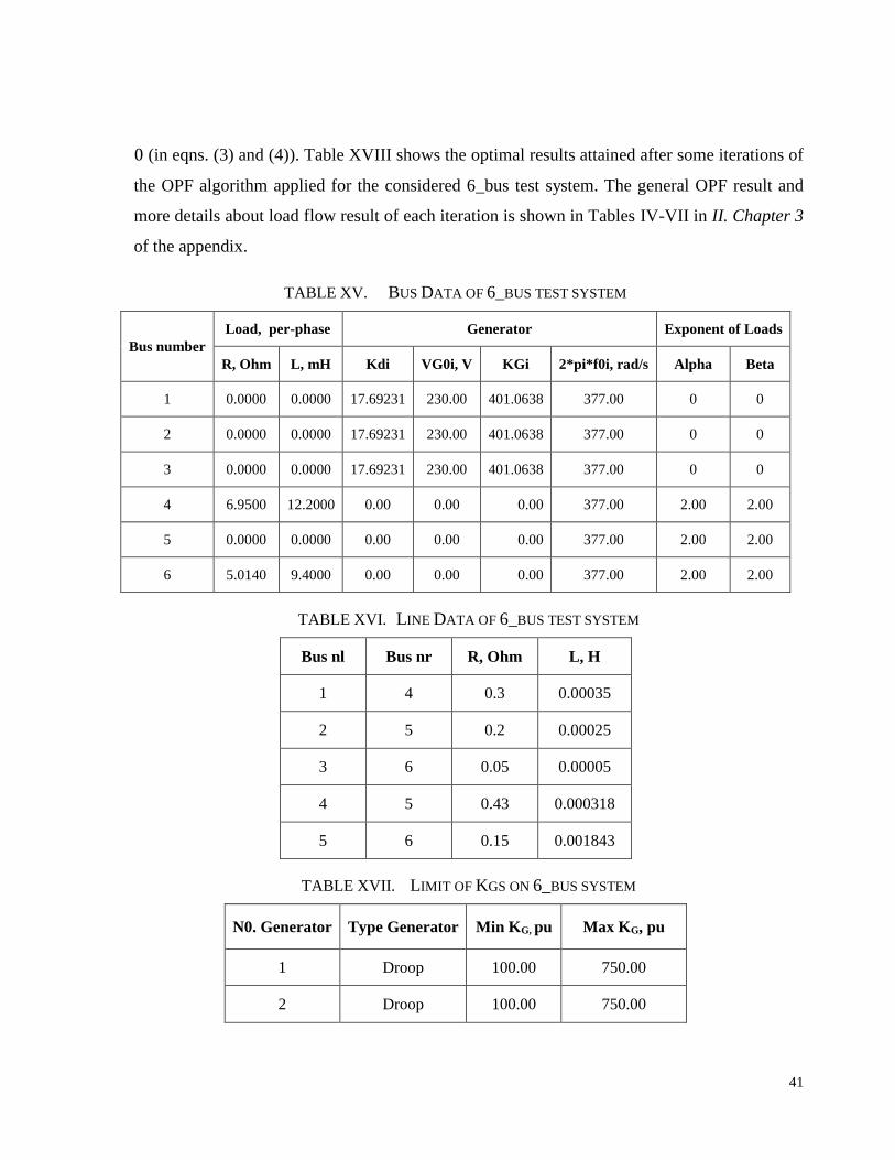
0 (in eqns. (3) and (4)). Table XVIII shows the optimal results attained after some iterations of
the OPF algorithm applied for the considered 6_bus test system. The general OPF result and
more details about load flow result of each iteration is shown in Tables IV-VII in II. Chapter 3
of the appendix.
TABLE XV. BUS DATA OF 6_BUS TEST SYSTEM
Bus number
Load, per-phase Generator Exponent of Loads
R, Ohm L, mH Kdi VG0i, V KGi 2*pi*f0i, rad/s Alpha Beta
1 0.0000 0.0000 17.69231 230.00 401.0638 377.00 0 0
2 0.0000 0.0000 17.69231 230.00 401.0638 377.00 0 0
3 0.0000 0.0000 17.69231 230.00 401.0638 377.00 0 0
4 6.9500 12.2000 0.00 0.00 0.00 377.00 2.00 2.00
5 0.0000 0.0000 0.00 0.00 0.00 377.00 2.00 2.00
6 5.0140 9.4000 0.00 0.00 0.00 377.00 2.00 2.00
TABLE XVI. LINE DATA OF 6_BUS TEST SYSTEM
Bus nl Bus nr R, Ohm L, H
1 4 0.3 0.00035
2 5 0.2 0.00025
3 6 0.05 0.00005
4 5 0.43 0.000318
5 6 0.15 0.001843
TABLE XVII. LIMIT OF KGS ON 6_BUS SYSTEM
N0. Generator Type Generator Min KG, pu Max KG, pu
1 Droop 100.00 750.00
2 Droop 100.00 750.00

42
N0. Generator Type Generator Min KG, pu Max KG, pu
3 Droop 100.00 750.00
TABLE XVIII. RESULT OF OPTIMAL LOAD FLOW ON 6_BUS SYSTEM, PU
Operating
point KG1 KG2 KG3 Ploss (calculated
by B coefficients)
Initial 401.0638 401.0638 401.0638 0.0265391
Optimal 406.3396 221.7403 573.4366 0.0228142
As it can be observed, for the considered loading condition, a reduction of 14.04% of power
losses is attained. Results of the same OPF procedure carried out for other loading conditions on
the same test system that can be experienced realistically (changing the load factor between 0.5
p.u. and 1 p.u.) still show a power losses reduction that does not go below 8% in all cases.
3.2.1. STABILITY ISSUES AND ARCHITECTURE OF THE CONTROL SYSTEM ON
6_BUS TEST SYSTEM
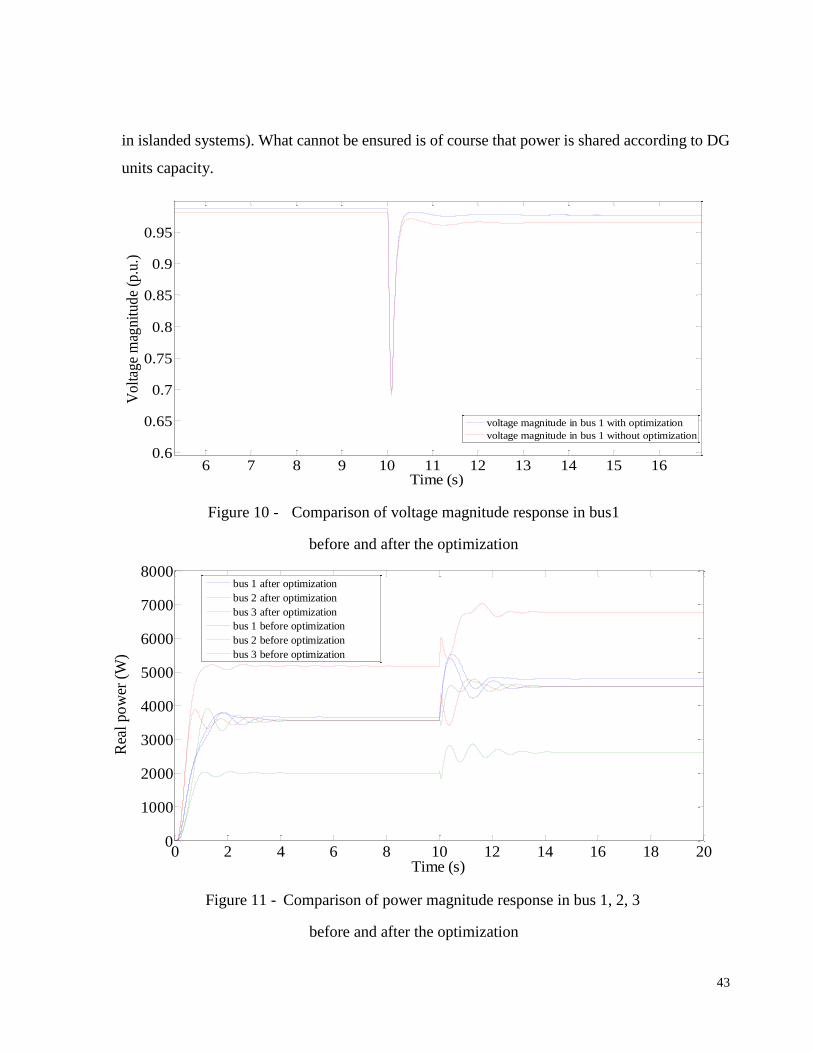
The dynamic behavior of the system with optimized parameters has been tested for a step
load change. At t = 10s, a three phase resistor branch (12Ω in each phase) and three phase
inductor branch (0.01H in each phase) is added to bus 4 and bus 6 by paralleling respectively.
The simulations, figures 10 and 11 show that the droop parameters found after the OPF
application produce stable results. As it was expected, the power sharing condition proposed by
the OPF solution increases the output power from the units (DG1 and DG3) that are electrically
closer to the loads that have increased their absorption and decreases the contribution from the
electrically farthest unit (DG2). Moreover the contextual variation of droop gains in the same
direction (increase for those that are closer and decrease for the farthest) implies and even more
reactive response if loads will keep varying in the same direction).
Stable behavior was expected since in [23] the stability margins are improved when: loading
is shared according to lines capacity and frequency is higher (consequence of lower power losses
43
in islanded systems). What cannot be ensured is of course that power is shared according to DG
units capacity.
Figure 10 - Comparison of voltage magnitude response in bus1
before and after the optimization
Figure 11 - Comparison of power magnitude response in bus 1, 2, 3
before and after the optimization
6 7 8 9 10 11 12 13 14 15 160.6
0.65
0.7
0.75
0.8
0.85
0.9
0.95
Time (s)
Volt
age
mag
nit
ud
e (p
.u.)
voltage magnitude in bus 1 with optimization
voltage magnitude in bus 1 without optimization
0 2 4 6 8 10 12 14 16 18 200
1000
2000
3000
4000
5000
6000
7000
8000
Time (s)
Rea
l p
ow
er (
W)
bus 1 after optimization
bus 2 after optimization
bus 3 after optimization
bus 1 before optimization
bus 2 before optimization
bus 3 before optimization

44
The application carried out even if for a simplified case (balanced loads) where only the P-f
droop parameters can be optimized shows the possibility to carry out a centralized and optimized
control of the system even when the grid is islanded. The load flow method, proposed in the
Chapter 2, for unbalanced systems can indeed be easily integrated into a heuristic-based OPF
giving rise to solution parameters both for P-f droop generation units and for Q-V droop
generation units.
The proposed OPF algorithm to be integrated into a centralized controller of a microgrid
would produce reduced losses and voltage drops all over the system. Moreover, if carried out
frequently, i.e. every few minutes, it eliminates the need for a distributed secondary regulation,
since it produces isofrequential, and within admissible rated bounds, operating points for all
droop interfaced generators.
The general architecture of the control system is therefore depicted in figure 12.
Figure 12 - General architecture of the control system

45
After a load variation and after the primary regulation, in order to compensate for the
frequency and amplitude deviations, the OPF is started. The frequency and voltage amplitude
levels in the microgrids f and V at all buses are sensed and compared with the references f*MG
and V*MG, if the errors are greater than a given threshold (which takes into account the
admissible frequency and voltage deviations), then the OPF is started again in order to restore
the operating voltage and frequency.
4. CONCLUSIONS
In this Chapter, a new OPF algorithm for islanded microgrids is proposed. The algorithm
produces a minimum losses and stable operating point with relevant droop parameters and solves
the OPF problem in closed form. It is interesting to point out that the underlying idea of a
centralized controller providing operating points at the same frequency and within admissible
bounds may lead to a simplified hierarchical structure only including two control levels (primary
and tertiary control levels). Nevertheless, at the moment the proposed algorithm cannot deal
with unbalanced loads and only outputs results for the P-f droops parameters, letting the Q-V
droops parameters non optimized.
The algorithm as it is proposed in this chapter is feasible for small systems where centralized
operation is possible and loads are typically balanced.

46
CHAPTER 4: OPTIMAL POWER FLOW BASED ON GLOW-
WORM SWARM OPTIMIZATION FOR THREE-PHASE
ISLANDED MICROGRIDS
1. INTRODUCTION
This Chapter presents an application of GSO method, to solve the OPF problem taking into
account the constraints of frequency and line ampacity in three-phase islanded Microgrids. Each
generation unit is equipped with a Power Electronics Interface. In the considered formulation,
the droop control parameters are considered as variables to be adjusted by a higher control level,
while the frequency is kept in rated bounds. Another typical constraint for OPF formulation, the
max ampacity of each line, is also considered. In this chapter, the authors compare a heuristic
method with a numerical method based on the Lagrange method and Trust region method to
solve the OPF in islanded migrogrids. As it will be shown, the numerical method does not allow
to take into account all the influential features of the OPF problem at hand. On the other hand,
a full study taking into account all influential features based on GSO method is also here
considered.
Some tests are executed on 6_bus LV systems with balanced loads, the results are compared
with those generated by a numerical method based on Lagrange multipliers in case of not taking
into account the constraints of frequency and line ampacity. Two case studies taking into account
the constraints of frequency and line ampacity with different dimensions and electrical features
have been considered and the obtained results show the efficiency of the proposed approach that
can be straightforward extended to unbalanced systems.
2. OPTIMAL POWER FLOW CALCULATION
The OPF in this work is solved to minimize power losses and the general model for OPF
calculation encompasses power lines, loads, generators, including their control loops such as
droop characteristics. The problem is highly non linear. The output variables are new droop
parameters for primary regulation, moreover the operating solution produces an iso-frequency
working condition for all units with operating frequency within admissible ranges. In [2] it has
been shown that the power losses term is connected to the droop parameters values and thus
such choice influences the steady state and dynamic operation of the microgrids.

47
2.1. OPTIMIZATION VARIABLES
In this chapter, both for P-f droop generation units and for Q-V droop generation units, the
optimization variables are the parameters of inverter interfaced units 𝐾𝐺 and 𝐾𝑑
𝐾𝐺 = (𝐾𝐺1, 𝐾𝐺2… ,𝐾𝐺𝑛𝑔 ) (71)
𝐾𝑑 = (𝐾𝑑1, 𝐾𝑑2… ,𝐾𝑑𝑛𝑔 ) (72)
where 𝑛𝑔 is the number of generators. Therefore the generated reactive and real powers 𝑃𝐺𝑖 and
𝑄𝐺𝑖 of generator i are respectively expressed as a linear function of voltage and frequency
displacements according to the terms (71) and (72). Their expression could be found in Chapter
II, equation (6), (7).
2.2. OBJECTIVE FUNCTION (OF)
Let 𝑃𝑖 denote the calculated three phase real power injected into the microgrid at bus i. The
formulation to calculate 𝑃𝑖 can be expressed, as follow:
𝑃𝑖(𝐾𝑔,𝐾𝑑) = ∑ |𝑉𝑖||𝑉𝑗||𝑌𝑖𝑗|𝑐𝑜𝑠(𝜃𝑖𝑗 − 𝛿𝑖 + 𝛿𝑗)𝑛𝑏𝑟𝑗=1 (73)
where:
𝑉𝑖 and 𝑉𝑗 are the voltages at bus 𝑖 and bus j, depending on 𝐾𝑔 and 𝐾𝑑 at droop buses.
𝛿𝑖 and 𝛿𝑗 are the phase angles of the voltages at bus 𝑖 and bus j, depending on 𝐾𝑔 and 𝐾𝑑 at
droop buses.
𝑌𝑖𝑗 is the admittance of branch 𝑖𝑗
𝜃𝑖𝑗 is the phase angle of 𝑌𝑖𝑗
𝑛𝑏𝑟 is the number of branch connected into bus 𝑖
So the total real power loss of the system or OF for three phases balanced system can be
calculated as follow:
𝑂𝐹(𝐾𝑔,𝐾𝑑) = 𝑃𝐿𝑜𝑠𝑠 = ∑ (𝑃𝑖(𝐾𝑔,𝐾𝑑))𝑛𝑏𝑢𝑠𝑖=1 (74)

48
where 𝑛𝑏𝑢𝑠 is the number of buses in system.
2.3. CONSTRAINTS
The optimal dispatch issue is that to find the set of droop parameters (𝐾𝐺𝑖) and (𝐾𝑑𝑖) and
relevant operating frequency and bus voltages minimizing the function expressed in (74), subject
to the constraint that generated power should equal total demands plus total power losses (𝑃𝐿𝑜𝑠𝑠):
∑ 𝑃𝐺𝑟𝑖 = ∑ 𝑃𝐿𝑖𝑛𝑑𝑖=1 + 𝑃𝐿𝑜𝑠𝑠
𝑛𝑔𝑟𝑖=1
(75)
where 𝑃𝐺𝑟𝑖 is the real power of generator i; 𝑃𝐿𝑖 is the real power of load bus i and 𝑛𝑑 is the
number of load buses.
Under the following inequality constraints, expressed as follows:
𝐾𝐺𝑖𝑚𝑖𝑛 ≤ 𝐾𝐺𝑖 ≤ 𝐾𝐺𝑖𝑚𝑎𝑥 , 𝑖 = 1 to 𝑛𝑔 (76)
𝐾𝑑𝑖𝑚𝑖𝑛 ≤ 𝐾𝑑𝑖 ≤ 𝐾𝑑𝑖𝑚𝑎𝑥, 𝑖 = 1 to 𝑛𝑔𝑟 (77)
∆𝑓 = 𝑓 − 𝑓0 ≤ 0.02 (78)
𝐼𝑏𝑟𝑎𝑛𝑐ℎ𝑖 ≤ 𝐼𝑚𝑎𝑥𝑏𝑟𝑎𝑛𝑐ℎ𝑖, 𝑖 = 1 to 𝑛𝑏𝑟 (79)
where 𝐾𝐺𝑖𝑚𝑖𝑛 , 𝐾𝐺𝑖𝑚𝑎𝑥 , 𝐾𝑑𝑖𝑚𝑖𝑛, 𝐾𝑑𝑖𝑚𝑎𝑥 respectively are the minimum and maximum values of
the droop parameters for P-f and Q-V droop generators. ∆𝑓 is the operating frequency deviation,
𝐼𝑏𝑟𝑎𝑛𝑐ℎ𝑖 is the current in the i-th branch and 𝐼𝑚𝑎𝑥𝑏𝑟𝑎𝑛𝑐ℎ𝑖 is the maximum current in the i-th
branch and 𝑛𝑏𝑟 is the number of branches in the system.
2.4. HEURISTIC GSO-BASED METHOD
The OF (74) for the considered OPF is highly non linear due to the non linear relation
between power losses and generated power. The variables (𝐾𝐺𝑖 and 𝐾𝑑𝑖) do not appear explicitly
in the equation but they are linearly related to the generated power. For this reason, the use of
classical non linear optimization methods seems to be inadequate due to the difficulty in
including constraints and unbalanced loading conditions.
Moreover, when the OF is highly nonlinear, the search space is typically multimodal. Hence
to analyze such complex model it is required to search for a global optimum. The global

49
optimization capability is important when dealing with complex nonlinear models and heuristics
can be a suitable choice.
GSO [25] is a relatively recent heuristic method. In GSO, agents are initially randomly
deployed in the objective function space. Each agent in the swarm decides the direction of
movement by the strength of the signal picked up from its neighbors. This is somewhat similar
to the luciferin induced glow of a glowworm which is used to attract mates or prey. The brighter
the glow, the more is the attraction. And the best will be chosen as the solution of problem.
Therefore, the glowworm metaphor is used to represent the underlying principles of this
optimization approach. In this chapter, this methodology solves the issue including constraints
about maximum frequency deviation and line ampacity limits to select the solution. Pseudocode
of the modified GSO algorithm considering frequency and line ampacity constraints is shown in
figure 13 below.
Figure 13 - Pseudocode of the GSO algorithm
When selecting solutions for recombination, those showing frequency and branch currents
out of bounds are still kept in the swarm, but are chosen with a lower probability. Fitness is
indeed based on ranking of solutions to keep a stable selection pressure in the probabilistic
choice of the target vector. Selection probability indeed depends on luciferin, which in turn
depends from fitness. For more details refer to [25].
Another issue usually faced when applying GSO is the choice of the Termination Condition.
It is difficult to know if the result attained at a given iteration is the best solution. To solve this
Initialize Archive A Repeat Until Termination Condition
Do m times Step 1: deterministic choice (selection) of the base vector Step 2: probabilistic choice (selection) of the target vector (Roulette
Wheel technique based on l(t)) considering frequency and line ampacity constraints
Step 3: recombination END m Step 4: create new population (replace A)
END A= archive m=archive size

50
issue, a number of iterations (n) is previously given as Termination Condition. The same
parameter n can be increased until results with no more improvements or negligible
improvements are attained.
3. APPLICATIONS
To assess the accuracy of GSO, it was compared to the Lagrange method, which is a
numerical method, as already described in Chapter 3 In order to perform the comparison both
constraints on frequency and line ampacity have been neglected and only Kgs have been
considered as optimization variables.
3.1. ACCURACY OF RESULTS
In Chapter III a numerical approach based on the Lagrange method is briefly described. It
solves the issue of optimal power flow on 3 phase balanced system with generators using inverter
interface units for droop regulation of V and f. The Kron’s loss formula was used to express the
power losses and thus only the KGs parameters could be optimized. A comparison about results
between Lagrange method and GSO method is done in this section on a 6_bus three phases
balanced LV system (figure 4) with ration R/X is around 2.5. The construction, parameters of
system and limits of KG are shown respectively in Tables I, II, III in III.1 Chapter 4 of appendix.
The results of the Lagrange method and GSO method are respectively shown in Table XIX and
Table XX. More details about optimal and load flow results are shown in III.1 Chapter 4 of
appendix.
TABLE XIX. RESULT OF OPTIMAL LOAD FLOW ON 6_BUS SYSTEM BY LAGRANGE METHOD
TAKING INTO ACCOUNT KGS, PU
KG1 KG2 KG3 Plossmin f
19.8331 10.3798 22.1034 0.0178887 1.0525
TABLE XX. RESULT OF OPTIMAL LOAD FLOW ON 6_BUS BALANCED SYSTEM BY GSO
HEURISTIC METHOD TAKING INTO ACCOUNT KGS, PU
Random KG1 KG2 KG3 Plossmin f
1 20.9933 10.0258 25.0000 0.0178565 1.0536

51
2 20.4090 9.7189 24.3476 0.0178565 1.0531
3 19.9132 9.5046 23.7349 0.0178565 1.0527
4 19.1041 9.1025 22.7901 0.0178565 1.0520
5 20.8797 9.9530 24.9023 0.0178565 1.0535
From Table XIX and Table XX, we can see that the minimum values of losses found by the
algorithms, Plossmin, are close, just 0.0000322 deviation between two cases.
The results of the heuristic for this problem could be considered reliable and repeatable. To
make sure of this 5 random independent runs of the GSO have been tried and the deviation of
results obtained is zero.
On the other hand, the sets of parameters outputted by the two algorithms are different. This
means that this OF is multimodal and there are some local maxima at close values.
3.2. OTHER APPLICATIONS WITH VARIABLE KGS AND KDS
In this section, an application of GSO Heuristic method, taking into account both KGs and
Kds, is shown on the same 6_bus test system that is operated in LV with the ration R/X is around
6.4. In this case, it was not possible to compare the results with the numerical method due to the
fact that Kds could not be optimized as in the Lagrange method.
In this case, due to the high R/X ratio, the virtual impedances at the droop buses was also
considered, such as it happens in low voltage systems. Virtual impedances are usually adopted
in addition to the conventional droop control of generators in order to improve system stability,
reactive power sharing performance and prevent power couplings which are caused by the
complex impedance in the parallel system [26-29]. The analysis about impacts of virtual
impedance to power flow calculation in LV microgrids is proposed in [30], where it is shown
the necessity of an accurate power flow analysis to evaluate the influence of frequency and
voltage droop gains, virtual impedance, nominal frequency and nominal voltage on the system
power flow by some case studies. The adoption of the virtual impedance in power flow
calculations is cleared out in figure 14 below.

52
Figure 14 - Virtual impedance control concept
In this way the two regulation channels can be considered as separated simplifying the
regulation architecture, and the 6_bus test system is turned on to 9_bus test system as in figure
15 below.
The parameters of 6_bus test system are shown in Tables XVII, XVIII and XIX in III.2
Chapter 4 of appendix. The optimal results after 5 random cases are shown in Table XXI. More
details about optimal result and load flow of each random are shown in III.2 Chapter 4 of
appendix.
Figure 15 - The 6_bus test system
TABLE XXI. RESULT OF OPTIMAL LOAD FLOW ON 6_BUS TEST SYSTEM TAKING INTO ACCOUNT KGS
AND KDS, PU

53
Random KG1 KG2 KG3 Kd1 Kd2 Kd3 Plossmin f
1 9.6625 8.9632 6.9471 6.0000 6.8368 15.6545 0.0001814 0.9949
2 10.2372 9.4079 7.3749 6.0000 6.1705 16.0000 0.0001814 0.9952
3 10.4711 9.6087 7.5745 6.0000 6.2901 16.0000 0.0001814 0.9953
4 10.3483 9.6237 7.3880 6.0113 8.0830 16.0000 0.0001815 0.9953
5 10.5047 9.6305 7.6456 6.0000 6.4065 15.9059 0.0001814 0.9953
From the Table XXI the optimal results of GSO method in 5 randoms are stable, the
deviation is only 0.0000001. So in next applications, we could only calculate OPF in 1 random
and the results could be believable.
3.3. APPLICATIONS CONSIDERING FREQUENCY AND LINE AMPACITY
CONSTRAINTS
3.3.1. APPLICATIONS WITH VARIABLES KGS
In this section, two test cases on a 6_bus balanced test system depicted in figure 4 are
presented. To simplify the problem and run a statistically significant sample (50) of test runs,
the two runs optimize only the KGi parameters and are referred to two different sets of line
ampacity of branches. The topological and electrical features of the system are shown in Tables
XXX and XXXI in III.3 Chapter 4 of appendix. Limits of KGs, line ampacities of two test cases
are shown in Table XXII, XXIII respectively. The load model used in this section depends on
voltage and frequency.
The results of the GSO method in the two cases are shown in Table XXIV. More details of
optimal result and power flow of two cases are shown in III.3 Chapter 4 of appendix.
Figure16 shows the OPF operating currents which are also compared with line ampacity on
each branch in the two cases.

54
TABLE XXII. LIMIT OF KGS ON 6_BUS TEST SYSTEM, TAKING INTO ACCOUNT CONSTRAINED
FREQUENCY AND LINE AMPACITY WITH VARIABLES ARE KGS, PU
Generators KGmin,pu KGmax,pu
G1 1 25
G2 1 25
G3 1 25
Where KGmin and Kgmax are minimum and maximum value of coefficient KG of
generators respectively.
TABLE XXIII. LINE AMPACITY OF BRANCHES ON 6_BUS SYSTEM OPTIMIZING KGS, PU
Branch
Imax, pu
Case 1 Case 2
L4_5 0.40 0.30
L1_4 0.50 0.47
L2_5 0.50 0.50
L6_5 0.40 0.30
L3_6 0.50 0.60
TABLE XXIV. RESULT OF OPTIMAL LOAD FLOW ON 6_BUS SYSTEM BY GSO HEURISTIC METHOD
TAKING INTO ACCOUNT KGS, PU
Case KG1 KG2 KG3 Plossmin f
1 8.7549 6.7822 7.2606 0.0352283 0.9808
2 7.6381 7.5541 7.9221 0.0359207 0.9814

55
Figure 16 - The OPF operating current in each branch in the two considered cases
In figure 16, Imax case 1 and Imax case 2 are the line ampacity on each branch of two test
cases; Iopt case1 and Iopt case2 are optimal currents on each branch of two test cases; L4_5,
L1_4, L2_5, L6_5 and L3_6 are branchs in 6_bus test system. From figure, we could see that at
each branch, the optimal currents are lower than the line ampacity in both of two test cases
except branch L1_4, the optimal current is equal to line ampacity. And in the table XXIV, the
Plossmin in case 2 is bigger than in case 1 as we reduce the line ampacity on branch L1_4. It
shows the resonable of the achieved results.
3.3.2. APPLICATION WITH VARIABLES KGS AND KDS
In this section, both sets of KGi and Kdi, are optimized. The load model used in this section
only depends on voltage (𝐾𝐺𝑓 = 𝐾𝑄𝑓 = 0). The limits of KGi and Kdi, are shown in Table XXV,
set of line ampacity of branches is similar to case 1 in Table XXII. The optimal power flow
results are shown in Table XXVI. More details of optimal result and optimal power flow are
shown in III.3 Chapter 4 of appendix. In all branches the OPF results produce similar current
flows as compared to those in figure16, see figure 17.
0.00
0.10
0.20
0.30
0.40
0.50
0.60
0.70
L4_5 L1_4 L2_5 L6_5 L3_6
Imax case 1, pu
I opt case1, pu
Imax case 2, pu
I opt case 2, pu

56
TABLE XXV. LIMITS OF KGS AND KDS ON 6_BUS BALANCED TEST SYSTEM OPTIMIZING KGS AND KDS, PU
Generators KGmin KGmax Kdmin Kdmax
G1 1 25 4 15
G2 1 25 4 15
G3 1 25 4 15
TABLE XXVI. RESULT OF OPTIMAL LOAD FLOW ON 6_BUS SYSTEM, OPTIMIZING KGS AND KDS, PU
KG1 KG2 KG3
Plossmin f 11.2421 9.4341 9.4641
Kd1 Kd2 Kd3 0.0351713 0.9926
4.3345 4.0099 4.3574
Figure 17 - The OPF operating current in each branch
Besides it can be observed that these flows are lower than the limit. In this application, the
set of line ampacity is the same with in 3.3.1-case 1, however we take into account more
0.0000
0.1000
0.2000
0.3000
0.4000
0.5000
0.6000
L4_5 L1_4 L2_5 L6_5 L3_6
Imax case 1, pu
I opt case1, pu

57
variables, both KGs ans Kds, the better operating point has been given with Plossmin in Table
XXVI is smaller than in 3.3.1-case 1 even that just small deviation (0.000057). The possibility
to optimize also the reactive power dispatch provides indeed more flexibility.
The attained results are reasonable and show that the proposed algorithm is effective, being
able to find a solution that satisfies the frequency and line ampacity constraints for a 6_bus test
system. All the reported results refer to a set of parameters showing the highest frequency of
occurrence within the considered sample of runs.
4. CONCLUSIONS
This chapter introduces an application of GSO method to solve the problem of OPF in
islanded three-phase microgrids. The system is supplied by inverter interfaced units with droop
controllers. Both P-f droops parameters and Q-V droops parameters are considered as variables
and constraints keep the current in branches below rated ampacity and frequency within given
bounds. Some tests are executed on 6_bus balanced systems to prove the efficiency of the
proposed approach. The flexibility of the considered solution approach allows the consideration
of unbalanced loads and further work will also be addressed to reduce calculation times.

58
CHAPTER V. CONCLUSIONS
This work has been focused on Optimal power flow issue in islanded microgrids in which
inverter interfaced units have an important role on operating and control. A load flow method
taking into account the model of these units has been used in this work to support the OPF both
using a numerical method and using a heuristic method.
The load flow solution uses a matlab solver, the results of applications on many kind of
islanded microgrid systems with different R/X ratios and sizes have shown the effectiveness and
correctness of the proposed method.
Then two original OPF methods, one based on a numerical approach and another based on
a heuristic approach, have been proposed to find out the optimal operating point for an islanded
MGs. The dependency in the modeling of all components on voltage and frequency allows to
use the OPF as a substitute of secondary regulation, provided it can be perfomed in reasonable
calculation times.
The numerical method uses a Lagrange approach. It has been applied on two islanded
microgrid test systems, 6_bus and 38_bus test system. The results have shown that this method
can give a good result on both low voltage and medium voltage systems and on various kind of
microgrid system in a few iterations and in limited running time. The application carried out, for
balanced loads and where only the P-f droop parameters can be optimized, shows the possibility
to carry out a centralized and optimized control of the system even when the grid is islanded.
The heuristic method is based on the Glow-worm Swarm optimizer. It effectively solves the
OPF and can account for constraints such as frequency in certain boundaries and line ampacity.
This method gives rise to solution parameters both for P-f droop generation units and for Q-V
droop generation units; it has been applied on 6_bus test system in many scenarios. The
application results have shown the effectiveness and correctness of it. However, the calculating
speed should be improved in the future to make it feasible for real world applications.

59
REFERENCS [1] J. M. Guerrero, J. C. Vásquez, J. Matas, L. G. de Vicuña, M. Castilla, “Hierarchical Control of
Droop-Controlled AC and DC Microgrids—A General Approach Towards Standardization”, 2011,
IEEE Trans on Industrial electronics, vol.58, issue 1 pp.158-172.
[2] Forner, D.; Erseghe, T.; Tomasin, S.; Tenti, P. “On efficient use of local sources in smart grids with
power quality constraints”. In Proceeding of the IEEE Int. Conf. Smart Grid Commun.,
Gaithersburg, MD, USA, Oct. 2010; pp. 555-560.
[3] Elrayyah, A.; Sozer, Y.; Elbuluk, M. “A Novel Load Flow Analysis for Particle-Swarm Optimized
Microgrid Power Sharing”. In Proceeding of the IEEE APEC; Long Beach, CA, USA. 2013; pp.
297-302.
[4] Sanseverino, E.R.; Di Silvestre, M.L.; Zizzo, G.; Gallea, R.; Quang, N.N. “A Self-Adapting
Approach for Forecast-Less Scheduling of Electrical Energy Storage Systems in a Liberalized
Energy Market”. Energies 2013, 6, 5738-5759.
[5] Lu, F.-C.; Hsu, Y. Y. “Fuzzy dynamic programming approach to reactive power/voltage control in
a distributionsubstation,” IEEE Trans. Power Syst. 1997, Volume 12, pp. 681–688.
[6] Levron, Y.; Guerrero, J.M; Beck, Y. “Optimal Power Flow in Microgrids With Energy Storage,”
IEEE Trans. Power Syst. 2013, Volume 28, pp. 3226-3234.
[7] Lam, A. Y. S.; Zhang, B.; Dominguez-Garcia, A.; Tse, D. “Optimal distributed voltage regulation
in power distribution networks”. http://arxiv.org/abs/1204.5226v1 (accessed in 2012).
[8] Lavaei, J.; Tse, D.; Zhang, B. “Geometry of power flows in tree networks”. In Proceeding of IEEE
Power Energy Soc. Gen. Meet., San Diego, CA, USA, Jul. 2012.
[9] Lu, D.; François, B. “Strategic Framework of an Energy Management of a Microgrid with a
Photovoltaic-Based Active Generator”. In Chapter ‘Electric Drives’ Joint Symposium, Proceedings
of IEEE Electromotion 2009 – EPE, Lille, France, 1-3 July 2009.
[10] Kanchev, H.; Lu, D.; Colas, F. ; Lazarov, V. ; Francois, B. “Energy Management and Operational
Planning of a Microgrid With a PV-Based Active Generator for Smart Grid Applications,” IEEE
Transactionson Industrial Electronics 2011, Volume 58, 4583-4592.

60
[11] Sanseverino, E. R.; Di Silvestre, M. L.; Ippolito, M. G.; De Paola, A.; Lo Re, G. “Execution,
monitoring and replanning approach for optimal energy management in microgrids”, Energy 2011,
Volume 36, 3429-3436.
[12] Di Silvestre, M. L.; Graditi, G.; Ippolito, M. G.; Sanseverino, E. R.; Zizzo, G. “Robust multi-
objective optimal dispatch of distributed energy resources in micro-grids”. In Proceeding of IEEE
Powertech 2011, Trondheim, Norway, June 2011, pp. 1-6.
[13] Corso, G.; Di Silvestre, M. L.; Ippolito, M. G.; Sanseverino, E. R.; Zizzo, G. “Multi-objective long
term optimal dispatch of distributed energy resources in micro-grids”. In Proceeding of Universities
Power Engineering Conference UPEC 2010, Cardiff, UK, September 2010, pp. 1-5.
[14] S. Bruno S., L. Silvia, R. Giuseppe, S. Ugo and M. La Scala “Unbalanced Three-Phase Optimal
Power Flow for Smart Grids”, IEEE Transactions on Industrial Electronics, VOL. 58, NO. 10,
OCTOBER 2011.
[15] S. Yan, S. Nai, and Y. Zhi, “Power Flow Calculation Method for Islanded Power Network”,
Proceedings of Asia Pacific Power and Energy Engineering Conference, APPEEC 2009, 27-31
March 2009, pp.1-5.
[16] T.L. Vandoorn, J.D.M. De Kooning, B. Meersman, J.M. Guerrero, and L. Vandevelde,“Automatic
Power-Sharing Modification of P/V Droop Controllers in Low-Voltage Resistive Microgrids” IEEE
Transactions on Power Delivery, Vol. 27, n. 4, Oct. 2012
[17] M. Morad, E. Hany, F.Ehab, and A. Yasser, “A Novel and Generalized Three-Phase Power Flow
Algorithm for Islanded Microgrids Using a Newton Trust Region Method”, IEEE Transactions on
Power system, Vol. 28, no. 1, February, 2013.
[18] W. H. Kersting, “Series impedance of overhead and underground lines”, in Distribution System
Modeling and Analysis. Boca Raton, FL: CRC, 2002, ch. $, pp. 77-108.
[19] IEEE Task Force on Load Representation for Dynamic Performance “Bibliography on load models
for power flow and dynamic performance simulation”, IEEE Transactions on Power systems, vol.
10, no. 1, pp 523-538, Feb. 1995
[20] P. Kundur, “Power system loads”, in Power System Stability and Control. New York: McGraw-
Hill, 1994, ch. 7, pp. 271-314.

61
[21] G. K. V. Raju and P. R. Bijwe, “Efficient reconfiguration of balanced and unbalanced distribution
systems for loss minimisation”, IET Gen., Transm., Distrib., vol.2, no. 1, pp 7-12, Jan. 2008.
[22] Y. Li and Y. Li, “Decoupled power control for an inverter based low voltage microgrid in
autonomous operation”, in Conf. Rec. IEEE International Power Electronics and Motion Control
Conference (IPEMC’09), Wuhan China, pp. 2490-2496, 2009.
[23] E. Barklund, Nagaraju Pogaku, Milan Prodanovic´, C. Hernandez-Aramburo, Member, IEEE, and
Tim C. Green, “Energy Management in Autonomous Microgrid Using Stability-Constrained Droop
Control of Inverters”, in IEEE TRANSACTIONS ON POWER ELECTRONICS, VOL. 23, NO. 5,
SEPTEMBER 2008.
[24] H. Saadat, “Derivation of Loss Formula”, in Power systems analysis. Singapore: McGraw-Hill,
1999, ch. 7, pp. 289-295.
[25] Krishnanand & Ghose, Glowworm Swarm Optimization (GSO), 2006.
[26] Jinwei He; Yun Wei Li, "Analysis, Design, and Implementation of Virtual Impedance for Power
Electronics Interfaced Distributed Generation," Industry Applications, IEEE Transactions on ,
vol.47, no.6, pp.2525,2538, Nov.-Dec. 2011
[27] Wei Yao; Min Chen; Matas, J.; Guerrero, J.M.; Zhao-ming Qian, "Design and Analysis of the Droop
Control Method for Parallel Inverters Considering the Impact of the Complex Impedance on the
Power Sharing," Industrial Electronics, IEEE Transactions on , vol.58, no.2, pp.576,588, Feb. 2011
[28] Jinwei He; Yun Wei Li; Guerrero, J.M.; Vasquez, J.C.; Blaabjerg, F., "An islanding microgrid
reactive power sharing scheme enhanced by programmed virtual impedances," Power Electronics
for Distributed Generation Systems (PEDG), 2012 3rd IEEE International Symposium on , vol., no.,
pp.229,235, 25-28 June 2012
[29] Matas J., Castilla M., García de Vicuna L., Miret J., and Vasquez J. C., “Virtual Impedance Loop
for Droop-Controlled Single-Phase Parallel Inverters Using a Second-Order General-Integrator
Scheme”, IEEE TRANSACTIONS ON POWER LECTRONICS, VOL. 25, NO. 12, DECEMBER
2010
[30] Li, C.; Chaudhary S.K.; Vasquez J. C.; and Guerrero, J.M., “Power Flow Analysis Algorithm for
Islanded LV Microgrids Including Distributed Generator Units with Droop Control and Virtual
Impedance Loop”, Proceedings of the 2014 IEEE PES General Meeting, 2014.
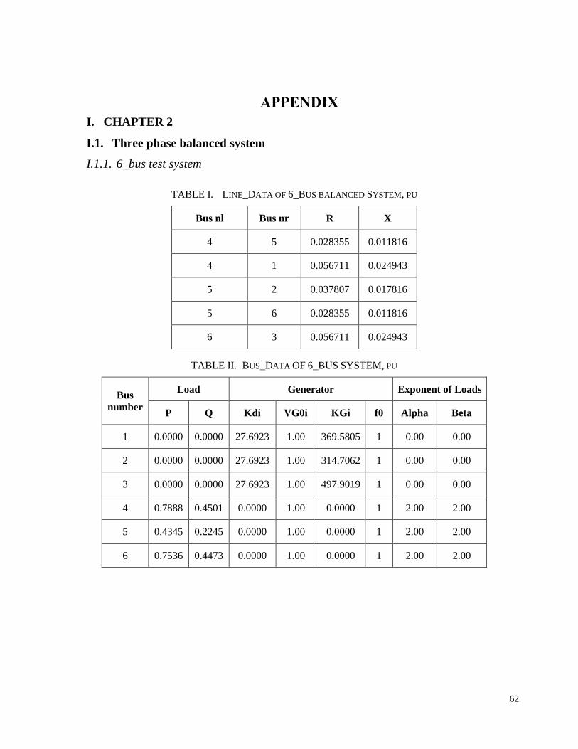
62
APPENDIX
I. CHAPTER 2
I.1. Three phase balanced system
I.1.1. 6_bus test system
TABLE I. LINE_DATA OF 6_BUS BALANCED SYSTEM, PU
Bus nl Bus nr R X
4 5 0.028355 0.011816
4 1 0.056711 0.024943
5 2 0.037807 0.017816
5 6 0.028355 0.011816
6 3 0.056711 0.024943
TABLE II. BUS_DATA OF 6_BUS SYSTEM, PU
Bus
number
Load Generator Exponent of Loads
P Q Kdi VG0i KGi f0 Alpha Beta
1 0.0000 0.0000 27.6923 1.00 369.5805 1 0.00 0.00
2 0.0000 0.0000 27.6923 1.00 314.7062 1 0.00 0.00
3 0.0000 0.0000 27.6923 1.00 497.9019 1 0.00 0.00
4 0.7888 0.4501 0.0000 1.00 0.0000 1 2.00 2.00
5 0.4345 0.2245 0.0000 1.00 0.0000 1 2.00 2.00
6 0.7536 0.4473 0.0000 1.00 0.0000 1 2.00 2.00

63
I.1.2. 16_bus test system
TABLE III. LINE_DATA OF 16_BUS BALANCED SYSTEM, PU
Bus nl Bus nr R X
1 4 0.012453 0.012453
4 5 0.006413 0.004608
5 6 0.006501 0.004608
6 7 0.001224 0.000405
4 8 0.00443 0.001464
8 9 0.003372 0.004439
8 10 0.001166 0.003853
10 11 0.002809 0.00192
11 12 0.00316 0.00161
11 13 0.005592 0.004415
13 2 0.003113 0.003113
10 14 0.00307 0.001564
14 15 0.004558 0.003574
14 16 0.001021 0.000974
16 3 0.003113 0.003113
TABLE IV. BUS_DATA OF 16_BUS SYSTEM, PU
Bus
number
Load Generator Exponent of Loads
P Q Kdi VG0i KGi f0 Alpha Beta
1 0.0000 0.0000 59.9880 1.00 607.2000 1 0.00 0.00
2 0.0000 0.0000 30.0030 1.00 311.7000 1 0.00 0.00
3 0.0000 0.0000 30.0000 1.00 1211.5000 1 0.00 0.00

64
Bus
number
Load Generator Exponent of Loads
P Q Kdi VG0i KGi f0 Alpha Beta
4 0.0600 0.0200 0.0000 0.00 0.0000 1 2.00 2.00
5 0.2000 0.1000 0.0000 0.00 0.0000 1 2.00 2.00
6 0.2000 0.1000 0.0000 0.00 0.0000 1 2.00 2.00
7 0.0450 0.0300 0.0000 0.00 0.0000 1 2.00 2.00
8 0.0600 0.0350 0.0000 0.00 0.0000 1 2.00 2.00
9 0.0600 0.0200 0.0000 0.00 0.0000 1 2.00 2.00
10 0.0600 0.0200 0.0000 0.00 0.0000 1 2.00 2.00
11 0.1200 0.0800 0.0000 0.00 0.0000 1 2.00 2.00
12 0.0600 0.0100 0.0000 0.00 0.0000 1 2.00 2.00
13 0.0600 0.0200 0.0000 0.00 0.0000 1 2.00 2.00
14 0.0900 0.0400 0.0000 0.00 0.0000 1 2.00 2.00
15 0.4200 0.2000 0.0000 0.00 0.0000 1 2.00 2.00
16 0.4200 0.2000 0.0000 0.00 0.0000 1 2.00 2.00
I.1.3. 38_bus test system
TABLE V. LINE_DATA OF 38_BUS BALANCED SYSTEM, PU
Bus nl Bus nr R X
6 35 0.000574 0.000293
35 36 0.00307 0.001564
36 37 0.002279 0.001161
37 38 0.002373 0.001209
38 34 0.0051 0.004402

65
Bus nl Bus nr R X
34 7 0.001166 0.003853
7 8 0.00443 0.001464
8 9 0.006413 0.004608
9 10 0.006501 0.004608
10 11 0.001224 0.000405
11 12 0.002331 0.000771
3 13 0.009141 0.007192
13 14 0.003372 0.004439
14 15 0.00368 0.003275
15 16 0.004647 0.003394
16 17 0.008026 0.010716
17 18 0.004558 0.003574
35 19 0.001021 0.000974
19 20 0.009366 0.00844
20 21 0.00255 0.002979
21 22 0.004414 0.005836
36 23 0.002809 0.00192
23 24 0.005592 0.004415
24 25 0.005579 0.004366
34 26 0.001264 0.000644
26 27 0.00177 0.000901
27 28 0.006594 0.005814
28 29 0.005007 0.004362

66
Bus nl Bus nr R X
29 30 0.00316 0.00161
30 31 0.006067 0.005996
31 32 0.001933 0.002253
32 33 0.002123 0.003301
8 1 0.012453 0.012453
29 2 0.012453 0.012453
12 3 0.012453 0.012453
22 4 0.003113 0.003113
25 5 0.003113 0.003113
TABLE VI. BUS_DATA OF 38_BUS SYSTEM, PU
Bus
number
Load Generator Exponent of Loads
P Q Kdi VG0i KGi f0 Alpha Beta
1 0.0000 0.0000 59.9880 1.01 394.0497 1 0.00 0.00
2 0.0000 0.0000 30.0030 1.01 294.0497 1 0.00 0.00
3 0.0000 0.0000 30.0000 1.01 214.0497 1 0.00 0.00
4 0.0000 0.0000 20.0000 1.01 214.0497 1 0.00 0.00
5 0.0000 0.0000 40.0000 1.01 294.0497 1 0.00 0.00
6 0.0000 0.0000 0.0000 0.00 0.0000 1 1.51 3.40
7 0.2000 0.1000 0.0000 0.00 0.0000 1 1.51 3.40
8 0.2000 0.1000 0.0000 0.00 0.0000 1 1.51 3.40
9 0.0600 0.0200 0.0000 0.00 0.0000 1 0.18 6.00
10 0.0600 0.0200 0.0000 0.00 0.0000 1 1.51 3.40

67
Bus
number
Load Generator Exponent of Loads
P Q Kdi VG0i KGi f0 Alpha Beta
11 0.0450 0.0300 0.0000 0.00 0.0000 1 1.51 3.40
12 0.0600 0.0350 0.0000 0.00 0.0000 1 0.92 4.04
13 0.0600 0.0350 0.0000 0.00 0.0000 1 1.51 3.40
14 0.1200 0.0800 0.0000 0.00 0.0000 1 0.92 4.04
15 0.0600 0.0100 0.0000 0.00 0.0000 1 1.51 3.40
16 0.0600 0.0200 0.0000 0.00 0.0000 1 0.18 6.00
17 0.0600 0.0200 0.0000 0.00 0.0000 1 1.51 3.40
18 0.0900 0.0400 0.0000 0.00 0.0000 1 0.18 6.00
19 0.0900 0.0400 0.0000 0.00 0.0000 1 0.92 4.04
20 0.0900 0.0400 0.0000 0.00 0.0000 1 1.51 3.40
21 0.0900 0.0400 0.0000 0.00 0.0000 1 0.18 6.00
22 0.0900 0.0400 0.0000 0.00 0.0000 1 0.92 4.04
23 0.0900 0.0500 0.0000 0.00 0.0000 1 1.51 3.40
24 0.4200 0.2000 0.0000 0.00 0.0000 1 1.51 3.40
25 0.4200 0.2000 0.0000 0.00 0.0000 1 1.51 3.40
26 0.0600 0.0250 0.0000 0.00 0.0000 1 1.51 3.40
27 0.0600 0.0250 0.0000 0.00 0.0000 1 0.18 6.00
28 0.0600 0.0200 0.0000 0.00 0.0000 1 1.51 3.40
29 0.1200 0.0700 0.0000 0.00 0.0000 1 1.51 3.40
30 0.2000 0.6000 0.0000 0.00 0.0000 1 1.51 3.40
31 0.1500 0.0700 0.0000 0.00 0.0000 1 0.92 4.04
32 0.2100 0.1000 0.0000 0.00 0.0000 1 0.92 4.04
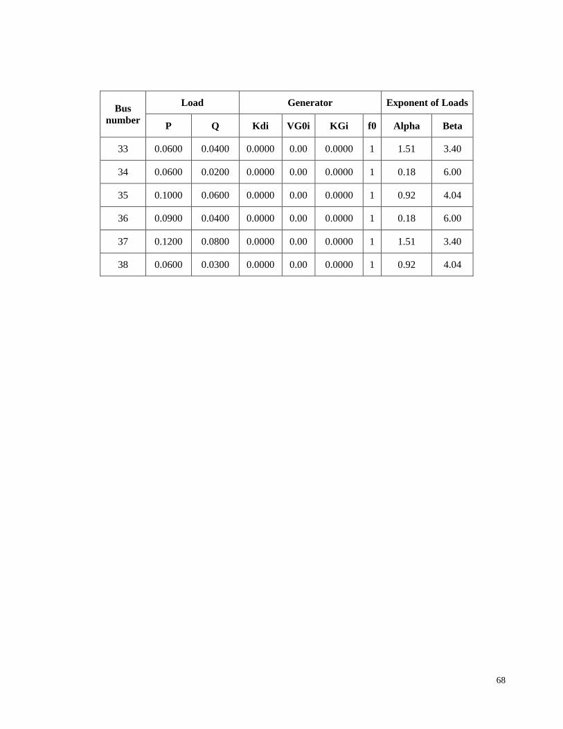
68
Bus
number
Load Generator Exponent of Loads
P Q Kdi VG0i KGi f0 Alpha Beta
33 0.0600 0.0400 0.0000 0.00 0.0000 1 1.51 3.40
34 0.0600 0.0200 0.0000 0.00 0.0000 1 0.18 6.00
35 0.1000 0.0600 0.0000 0.00 0.0000 1 0.92 4.04
36 0.0900 0.0400 0.0000 0.00 0.0000 1 0.18 6.00
37 0.1200 0.0800 0.0000 0.00 0.0000 1 1.51 3.40
38 0.0600 0.0300 0.0000 0.00 0.0000 1 0.92 4.04

69
I.2. Three phase unbalanced system
I.2.1. Data of 25_bus test system
TABLE VII. LINE DATA OF 25_BUS SYSTEM, IMPEDANCE FOR DIFERENT TYPE OF CONDUCTOR ARE
SHOWN BELOW THIS TABLE
Bus nl Bus nr Length, ft Length, mile Conductor
type
1 2 1000 0.18939394 1
2 3 500 0.09469697 1
2 6 500 0.09469697 2
3 4 500 0.09469697 1
3 18 500 0.09469697 2
4 5 500 0.09469697 2
4 23 400 0.07575758 2
6 7 500 0.09469697 2
6 8 1000 0.18939394 2
7 9 500 0.09469697 2
7 14 500 0.09469697 2
7 16 500 0.09469697 2
9 10 500 0.09469697 2
10 11 300 0.05681818 2
11 12 200 0.03787879 2
11 13 200 0.03787879 2
14 15 300 0.05681818 2
14 17 300 0.05681818 2
18 20 500 0.09469697 2

70
Bus nl Bus nr Length, ft Length, mile Conductor
type
18 21 400 0.07575758 2
20 19 400 0.07575758 2
21 22 400 0.07575758 2
23 24 400 0.07575758 2
24 25 400 0.07575758 2
5 22 400 0.07575758 2
15 8 300 0.05681818 2
12 25 500 0.09469697 3
Impedance for type 1 of conductors, ohms/mile
Z1 = [0.3686+1i*0.6852 0.0169+1i*0.1515 0.0155+1i*0.1098
0.0169+1i*0.1515 0.3757+1i*0.6715 0.0188+1i*0.2072
0.0155+1i*0.1098 0.0188+1i*0.2072 0.3723+1i*0.6782];
Impedance for type 2 of conductors, ohms/mile
Z2 = [0.9775+1i*0.8717 0.0167+1i*0.1697 0.0152+1i*0.1264
0.0167+1i*0.1697 0.9844+1i*0.8654 0.0186+1i*0.2275
0.0152+1i*0.1264 0.0186+1i*0.2275 0.9810+1i*0.8648];
Impedance for type 3 of conductors, ohms/mile
Z3 = [1.9280+1i*1.4194 0.0161+1i*0.1183 0.0161+1i*0.1183
0.0161+1i*0.1183 1.9308+1i*1.4215 0.0161+1i*0.1183
0.0161+1i*0.1183 0.0161+1i*0.1183 1.9337+1i*1.4236];

71
TABLE VIII. BUS DATA OF 25_BUS SYSTEM
Bus
number
Load phase A, kW Load phase B, kW Load phase C, kW Generator Exponent of Loads
P Q P Q P Q Kdi 𝐕𝟎𝐢, pu KGi f0i, pu α β
1 0.00 0.00 0.00 0.00 0.00 0.00 0.00 0.00 0.00 1.000 0.00 0.00
2 0.00 0.00 0.00 0.00 0.00 0.00 0.00 0.00 0.00 1.000 0.00 0.00
3 35.00 25.00 40.00 30.00 45.00 32.00 0.00 0.00 0.00 1.000 0.18 6.00
4 50.00 40.00 60.00 45.00 70.00 35.00 0.00 0.00 0.00 1.000 1.51 3.40
5 40.00 30.00 37.00 28.00 50.00 32.00 0.00 0.00 0.00 1.000 0.92 4.04
6 40.00 20.00 45.00 32.00 35.00 25.00 0.00 0.00 0.00 1.000 0.18 6.00
7 0.00 0.00 0.00 0.00 0.00 0.00 0.00 0.00 0.00 1.000 1.51 3.40
8 35.00 10.00 45.00 32.00 40.00 28.00 0.00 0.00 0.00 1.000 1.51 3.40
9 60.00 45.00 50.00 40.00 50.00 35.00 0.00 0.00 0.00 1.000 0.18 6.00
10 35.00 25.00 40.00 30.00 45.00 32.00 0.00 0.00 0.00 1.000 1.51 3.40
11 45.00 25.00 35.00 20.00 40.00 26.00 0.00 0.00 0.00 1.000 1.51 3.40
12 50.00 35.00 60.00 45.00 70.00 40.00 0.00 0.00 0.00 1.000 0.92 4.04
13 35.00 25.00 45.00 32.00 40.00 30.00 5.00 1.04 10.00 1.002 1.51 3.40
14 50.00 20.00 60.00 25.00 70.00 35.00 0.00 0.00 0.00 1.000 0.92 4.04
15 133.30 50.00 100.00 25.00 75.00 30.00 0.00 0.00 0.00 1.000 1.51 3.40

72
16 45.00 15.00 35.00 20.00 50.00 26.00 0.00 0.00 0.00 1.000 0.18 6.00
17 40.00 10.00 35.00 8.00 50.00 15.00 0.00 0.00 0.00 1.000 1.51 3.40
18 35.00 25.00 40.00 30.00 45.00 32.00 0.00 0.00 0.00 1.000 0.18 6.00
19 60.00 45.00 50.00 35.00 50.00 40.00 10.00 1.05 10.00 1.002 0.92 4.04
20 40.00 30.00 35.00 25.00 45.00 32.00 0.00 0.00 0.00 1.000 1.51 3.40
21 50.00 35.00 40.00 33.00 45.00 36.00 0.00 0.00 0.00 1.000 0.18 6.00
22 50.00 35.00 60.00 45.00 70.00 40.00 0.00 0.00 0.00 1.000 0.92 4.04
23 60.00 45.00 50.00 40.00 70.00 35.00 0.00 0.00 0.00 1.000 1.51 3.40
24 35.00 25.00 40.00 30.00 50.00 32.00 0.00 0.00 0.00 1.000 1.51 3.40
25 60.00 45.00 50.00 30.00 40.00 35.00 5.00 1.04 20.00 1.002 1.51 3.40

73
I.2.2. Changing KG13
TABLE IX. VOLTAGE PROFILE AND LOADS RESULTS OF THE PROPOSED POWER FLOW IN 25-BUS UNBALANCED TEST SYSTEM, KG13=20
Bus n0
Phase A Phase B Phase C
Van (pu,rad) Load (pu) Vbn (pu,rad) Load (pu) Vcn (pu,rad) Load (pu)
Mag Agl P Q Mag Agl P Q Mag Agl P Q
1 0.9763 0.0000 0.0000 0.0000 0.9735 -2.0876 0.0000 0.0000 0.9739 2.0937 0.0000 0.0000
2 0.9763 0.0000 0.0000 0.0000 0.9735 -2.0876 0.0000 0.0000 0.9739 2.0937 0.0000 0.0000
3 0.9769 0.0000 0.0012 0.0007 0.9740 -2.0876 0.0013 0.0009 0.9744 2.0936 0.0015 0.0009
4 0.9771 0.0005 0.0016 0.0012 0.9742 -2.0874 0.0019 0.0014 0.9746 2.0939 0.0022 0.0011
5 0.9734 -0.0026 0.0013 0.0009 0.9702 -2.0903 0.0012 0.0008 0.9701 2.0901 0.0016 0.0009
6 0.9651 0.0038 0.0013 0.0005 0.9628 -2.0809 0.0015 0.0009 0.9643 2.1003 0.0012 0.0007
7 0.9650 0.0097 0.0000 0.0000 0.9637 -2.0743 0.0000 0.0000 0.9643 2.1069 0.0000 0.0000
8 0.9571 0.0024 0.0011 0.0003 0.9552 -2.0805 0.0014 0.0009 0.9574 2.1008 0.0012 0.0008
9 0.9778 0.0219 0.0020 0.0013 0.9773 -2.0646 0.0017 0.0012 0.9780 2.1181 0.0017 0.0010
10 0.9960 0.0339 0.0012 0.0008 0.9953 -2.0553 0.0013 0.0010 0.9956 2.1293 0.0015 0.0011
11 1.0173 0.0454 0.0015 0.0009 1.0170 -2.0466 0.0012 0.0007 1.0170 2.1404 0.0014 0.0009
12 1.0204 0.0399 0.0017 0.0013 1.0192 -2.0529 0.0020 0.0016 1.0193 2.1346 0.0024 0.0014
13 1.0394 0.0624 0.0012 0.0010 1.0394 -2.0320 0.0016 0.0012 1.0394 2.1568 0.0014 0.0011
14 0.9552 0.0047 0.0016 0.0006 0.9538 -2.0775 0.0019 0.0007 0.9545 2.1032 0.0022 0.0010

74
Bus n0
Phase A Phase B Phase C
Van (pu,rad) Load (pu) Vbn (pu,rad) Load (pu) Vcn (pu,rad) Load (pu)
Mag Agl P Q Mag Agl P Q Mag Agl P Q
15 0.9514 0.0018 0.0041 0.0014 0.9513 -2.0801 0.0031 0.0010 0.9533 2.1017 0.0023 0.0011
16 0.9620 0.0084 0.0015 0.0004 0.9609 -2.0745 0.0012 0.0005 0.9607 2.1058 0.0017 0.0007
17 0.9528 0.0035 0.0012 0.0003 0.9508 -2.0772 0.0011 0.0007 0.9506 2.1025 0.0015 0.0009
18 0.9848 -0.0108 0.0012 0.0008 0.9820 -2.0999 0.0013 0.0009 0.9817 2.0833 0.0015 0.0010
19 1.0460 -0.0472 0.0021 0.0018 1.0460 -2.1416 0.0017 0.0014 1.0460 2.0472 0.0017 0.0016
20 1.0037 -0.0236 0.0013 0.0010 1.0018 -2.1151 0.0012 0.0008 1.0005 2.0721 0.0015 0.0011
21 0.9768 -0.0084 0.0017 0.0010 0.9740 -2.0965 0.0013 0.0009 0.9737 2.0850 0.0015 0.0010
22 0.9730 -0.0055 0.0016 0.0010 0.9694 -2.0933 0.0019 0.0013 0.9694 2.0869 0.0023 0.0012
23 0.9916 0.0104 0.0020 0.0015 0.9899 -2.0794 0.0016 0.0013 0.9898 2.1031 0.0023 0.0011
24 1.0114 0.0199 0.0012 0.0009 1.0103 -2.0721 0.0014 0.0010 1.0100 2.1132 0.0017 0.0011
25 1.0343 0.0289 0.0021 0.0017 1.0343 -2.0655 0.0017 0.0011 1.0343 2.1233 0.0014 0.0013
Total PLa QLa PLb QLb PLc QLc PLtotal QLtotal f/pu Ploss Vmin/pu Vmax/pu
0.0357 0.0212 0.0346 0.0223 0.0377 0.0377 0.1080 0.0812 0.9997 0.0075 0.9506 1.0460

75
TABLE X. DG UNITS REAL AND REACTIVE POWER GENERATION IN 25-BUS UNBALANCED TEST SYSTEM, KG13=20
Busid(DG) PGa PGb PGc QGa QGb QGc
13 0.0150 0.0150 0.0162 0.0006 0.0009 0.0015
19 0.0078 0.0074 0.0079 0.0132 0.0136 0.0137
25 0.0152 0.0148 0.0162 0.0091 0.0094 0.0098
TABLE XI. VOLTAGE PROFILE AND LOADS RESULTS OF THE PROPOSED POWER FLOW IN 25-BUS UNBALANCED TEST
SYSTEM, KG13=30
Bus n0
Phase A Phase B Phase C
Van (pu,rad) Load (pu) Vbn (pu,rad) Load (pu) Vcn (pu,rad) Load (pu)
Mag Agl P Q Mag Agl P Q Mag Agl P Q
1 0.9751 0.0000 0.0000 0.0000 0.9720 -2.0876 0.0000 0.0000 0.9727 2.0941 0.0000 0.0000
2 0.9751 0.0000 0.0000 0.0000 0.9720 -2.0876 0.0000 0.0000 0.9727 2.0941 0.0000 0.0000
3 0.9758 -0.0002 0.0012 0.0007 0.9762 -2.0880 0.0013 0.0008 0.0973 2.0937 0.0015 0.0009
4 0.9760 0.0002 0.0016 0.0012 0.9728 -2.0876 0.0019 0.0014 0.9736 2.0940 0.0022 0.0011
5 0.9722 -0.0038 0.0013 0.0009 0.9688 -2.0915 0.0012 0.0008 0.9690 2.0893 0.0016 0.0009
6 0.9641 0.0085 0.0013 0.0005 0.9616 -2.0762 0.0015 0.0008 0.9634 2.1054 0.0012 0.0007
7 0.9642 0.0183 0.0000 0.0000 0.9627 -2.0657 0.0000 0.0000 0.9637 2.1159 0.0000 0.0000
8 0.9562 0.0081 0.0011 0.0003 0.9540 -2.0747 0.0014 0.0009 0.9565 2.1068 0.0012 0.0008
9 0.9774 0.0352 0.0020 0.0013 0.9767 -2.0512 0.0017 0.0012 0.9777 2.1318 0.0017 0.0010
10 0.9961 0.0518 0.0012 0.0008 0.9952 -2.0373 0.0013 0.0010 0.9959 2.1476 0.0015 0.0011
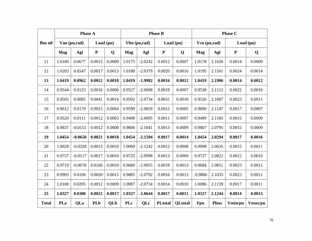
76
Bus n0
Phase A Phase B Phase C
Van (pu,rad) Load (pu) Vbn (pu,rad) Load (pu) Vcn (pu,rad) Load (pu)
Mag Agl P Q Mag Agl P Q Mag Agl P Q
11 1.0180 0.0677 0.0015 0.0009 1.0175 -2.0242 0.0012 0.0007 1.0178 2.1630 0.0014 0.0009
12 1.0203 0.0547 0.0017 0.0013 1.0188 -2.0379 0.0020 0.0016 1.0195 2.1501 0.0024 0.0014
13 1.0419 0.0962 0.0012 0.0010 1.0419 -1.9982 0.0016 0.0012 1.0419 2.1906 0.0014 0.0012
14 0.9544 0.0123 0.0016 0.0006 0.9527 -2.0698 0.0019 0.0007 0.9538 2.1112 0.0022 0.0010
15 0.9505 0.0085 0.0041 0.0014 0.9502 -2.0734 0.0031 0.0010 0.9526 2.1087 0.0023 0.0011
16 0.9612 0.0170 0.0015 0.0004 0.9599 -2.0659 0.0012 0.0005 0.9600 2.1147 0.0017 0.0007
17 0.9520 0.0111 0.0012 0.0003 0.9498 -2.0695 0.0011 0.0007 0.9499 2.1105 0.0015 0.0009
18 0.9837 -0.0151 0.0012 0.0008 0.9806 -2.1041 0.0013 0.0009 0.9807 2.0795 0.0015 0.0009
19 1.0454 -0.0650 0.0021 0.0018 1.0454 -2.1594 0.0017 0.0014 1.0454 2.0294 0.0017 0.0016
20 1.0028 -0.0328 0.0013 0.0010 1.0004 -2.1242 0.0012 0.0008 0.9998 2.0635 0.0015 0.0011
21 0.9757 -0.0117 0.0017 0.0010 0.9725 -2.0998 0.0013 0.0009 0.9727 2.0822 0.0015 0.0010
22 0.9719 -0.0078 0.0160 0.0010 0.9680 -2.0955 0.0019 0.0013 0.9684 2.0851 0.0023 0.0012
23 0.9903 0.0106 0.0020 0.0015 0.9885 -2.0792 0.0016 0.0013 .0.9886 2.1035 0.0023 0.0011
24 1.0100 0.0205 0.0012 0.0009 1.0087 -2.0714 0.0014 0.0010 1.0086 2.1139 0.0017 0.0011
25 1.0327 0.0300 0.0021 0.0017 1.0327 -2.0644 0.0017 0.0011 1.0327 2.1244 0.0014 0.0013
Total PLa QLa PLb QLb PLc QLc PLtotal QLtotal f/pu Ploss Vmin/pu Vmax/pu

77
Bus n0
Phase A Phase B Phase C
Van (pu,rad) Load (pu) Vbn (pu,rad) Load (pu) Vcn (pu,rad) Load (pu)
Mag Agl P Q Mag Agl P Q Mag Agl P Q
0.0357 0.0211 0.0346 0.0222 0.0377 0.0377 0.1080 0.0810 1.0000 0.0101 0.0973 1.0454
TABLE XII. DG UNITS REAL AND REACTIVE POWER GENERATION IN 25-BUS UNBALANCED TEST SYSTEM, KG13=30
Busid(DG) PGa PGb PGc QGa QGb QGc
13 0.0192 0.0190 0.0207 -0.0034 -0.0034 -0.0026
19 0.0067 0.0064 0.0066 0.0151 0.0156 0.0157
25 0.0130 0.0126 0.0137 0.0117 0.0121 0.0125
TABLE XIII. VOLTAGE PROFILE AND LOADS RESULTS OF THE PROPOSED POWER FLOW IN 25-BUS UNBALANCED TEST
SYSTEM, KG25=30
Bus n0
Phase A Phase B Phase C
Van (pu,rad) Load (pu) Vbn (pu,rad) Load (pu) Vcn (pu,rad) Load (pu)
Mag Agl P Q Mag Agl P Q Mag Agl P Q
1 0.9777 0.0000 0.0000 0.0000 0.9750 -2.0876 0.0000 0.0000 0.9752 2.0934 0.0000 0.0000
2 0.9777 0.0000 0.0000 0.0000 0.9750 -2.0876 0.0000 0.0000 0.9752 2.0934 0.0000 0.0000
3 0.9783 0.0003 0.0012 0.0007 0.9755 -2.0875 0.0013 0.0009 0.9757 2.0936 0.0015 0.0009
4 0.9784 0.0011 0.0016 0.0012 0.9757 -2.0869 0.0019 0.0014 0.9758 2.0942 0.0022 0.0011
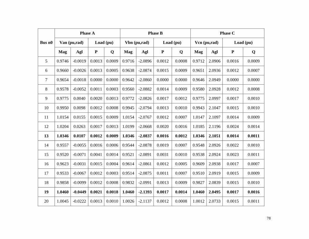
78
Bus n0
Phase A Phase B Phase C
Van (pu,rad) Load (pu) Vbn (pu,rad) Load (pu) Vcn (pu,rad) Load (pu)
Mag Agl P Q Mag Agl P Q Mag Agl P Q
5 0.9746 -0.0019 0.0013 0.0009 0.9716 -2.0896 0.0012 0.0008 0.9712 2.0906 0.0016 0.0009
6 0.9660 -0.0026 0.0013 0.0005 0.9638 -2.0874 0.0015 0.0009 0.9651 2.0936 0.0012 0.0007
7 0.9654 -0.0018 0.0000 0.0000 0.9642 -2.0860 0.0000 0.0000 0.9646 2.0949 0.0000 0.0000
8 0.9578 -0.0052 0.0011 0.0003 0.9560 -2.0882 0.0014 0.0009 0.9580 2.0928 0.0012 0.0008
9 0.9775 0.0040 0.0020 0.0013 0.9772 -2.0826 0.0017 0.0012 0.9775 2.0997 0.0017 0.0010
10 0.9950 0.0098 0.0012 0.0008 0.9945 -2.0794 0.0013 0.0010 0.9943 2.1047 0.0015 0.0010
11 1.0154 0.0155 0.0015 0.0009 1.0154 -2.0767 0.0012 0.0007 1.0147 2.1097 0.0014 0.0009
12 1.0204 0.0263 0.0017 0.0013 1.0199 -2.0668 0.0020 0.0016 1.0185 2.1196 0.0024 0.0014
13 1.0346 0.0107 0.0012 0.0009 1.0346 -2.0837 0.0016 0.0012 1.0346 2.1051 0.0014 0.0011
14 0.9557 -0.0055 0.0016 0.0006 0.9544 -2.0878 0.0019 0.0007 0.9548 2.0926 0.0022 0.0010
15 0.9520 -0.0071 0.0041 0.0014 0.9521 -2.0891 0.0031 0.0010 0.9538 2.0924 0.0023 0.0011
16 0.9623 -0.0031 0.0015 0.0004 0.9614 -2.0861 0.0012 0.0005 0.9609 2.0938 0.0017 0.0007
17 0.9533 -0.0067 0.0012 0.0003 0.9514 -2.0875 0.0011 0.0007 0.9510 2.0919 0.0015 0.0009
18 0.9858 -0.0099 0.0012 0.0008 0.9832 -2.0991 0.0013 0.0009 0.9827 2.0839 0.0015 0.0010
19 1.0460 -0.0449 0.0021 0.0018 1.0460 -2.1393 0.0017 0.0014 1.0460 2.0495 0.0017 0.0016
20 1.0045 -0.0222 0.0013 0.0010 1.0026 -2.1137 0.0012 0.0008 1.0012 2.0733 0.0015 0.0011

79
Bus n0
Phase A Phase B Phase C
Van (pu,rad) Load (pu) Vbn (pu,rad) Load (pu) Vcn (pu,rad) Load (pu)
Mag Agl P Q Mag Agl P Q Mag Agl P Q
21 0.9779 -0.0076 0.0017 0.0010 0.9752 -2.0957 0.0013 0.0009 0.9747 2.0856 0.0015 0.0010
22 0.9742 -0.0048 0.0016 0.0010 0.9707 -2.0926 0.0019 0.0013 0.9705 2.0875 0.0023 0.0012
23 0.9939 0.0165 0.0020 0.0015 0.9923 -2.0733 0.0016 0.0013 0.9920 2.1091 0.0023 0.0011
24 1.0148 0.0313 0.0012 0.0009 1.0137 -2.0606 0.0014 0.0010 1.0134 2.1246 0.0017 0.0011
25 1.0389 0.0454 0.0021 0.0017 1.0389 -2.0490 0.0018 0.0011 1.0389 2.1398 0.0014 0.0013
Total PLa QLa PLb QLb PLc QLc PLtotal QLtotal f/pu Ploss Vmin/pu Vmax/pu
0.0357 0.0213 0.0347 0.0223 0.0377 0.0377 0.1081 0.0813 0.9997 0.0074 0.9510 1.0460
TABLE XIV. DG UNITS REAL AND REACTIVE POWER GENERATION IN 25-BUS UNBALANCED TEST SYSTEM, KG25=30
Busid(DG) PGa PGb PGc QGa QGb QGc
13 0.0075 0.0076 0.0080 0.0084 0.0091 0.0096
19 0.0078 0.0074 0.0079 0.0129 0.0133 0.0134
25 0.0228 0.0221 0.0244 0.0017 0.0016 0.0020

80
TABLE XV. VOLTAGE PROFILE AND LOADS RESULTS OF THE PROPOSED POWER FLOW IN 25-BUS UNBALANCED TEST
SYSTEM, KG25=40
Bus n0
Phase A Phase B Phase C
Van (pu,rad) Load (pu) Vbn (pu,rad) Load (pu) Vcn (pu,rad) Load (pu)
Mag Agl P Q Mag Agl P Q Mag Agl P Q
1 0.9776 0.0000 0.0000 0.0000 0.9748 -2.0876 0.0000 0.0000 0.9753 2.0937 0.0000 0.0000
2 0.9776 0.0000 0.0000 0.0000 0.9748 -2.0876 0.0000 0.0000 0.9753 2.0937 0.0000 0.0000
3 0.9782 0.0003 0.0012 0.0007 0.9753 -2.0875 0.0013 0.0009 0.9757 2.0939 0.0015 0.0009
4 0.9783 0.0013 0.0016 0.0012 0.9754 -2.0867 0.0019 0.0014 0.9758 2.0946 0.0022 0.0011
5 0.9744 -0.0027 0.0013 0.0009 0.9713 -2.0904 0.0012 0.0008 0.9712 2.0900 0.0016 0.0009
6 0.9658 -0.0022 0.0013 0.0005 0.9636 -2.0870 0.0015 0.0009 0.9650 2.0941 0.0012 0.0007
7 0.9652 -0.0011 0.0000 0.0000 0.9640 -2.0853 0.0000 0.0000 0.9645 2.0957 0.0000 0.0000
8 0.9577 -0.0048 0.0011 0.0003 0.9558 -2.0877 0.0014 0.0009 0.9579 2.0934 0.0012 0.0008
9 0.9773 0.0050 0.0020 0.0013 0.9770 -2.0816 0.0017 0.0012 0.9773 2.1008 0.0017 0.0010
10 0.9947 0.0112 0.0012 0.0008 0.9943 -2.0780 0.0013 0.0010 0.9940 2.1060 0.0015 0.0010
11 1.0151 0.0172 0.0015 0.0009 1.0152 -2.0749 0.0012 0.0007 1.0143 2.1114 0.0014 0.0009
12 1.0206 0.0319 0.0017 0.0013 1.0203 -2.0613 0.0020 0.0016 1.0186 2.1249 0.0024 0.0014
13 1.0338 0.0090 0.0012 0.0009 1.0338 -2.0854 0.0016 0.0012 1.0338 2.1034 0.0014 0.0011
14 0.9556 -0.0050 0.0016 0.0006 0.9542 -2.0872 0.0019 0.0007 0.9547 2.0933 0.0022 0.0010
15 0.9518 -0.0066 0.0041 0.0014 0.9519 -2.0885 0.0031 0.0010 0.9537 2.0930 0.0023 0.0011

81
Bus n0
Phase A Phase B Phase C
Van (pu,rad) Load (pu) Vbn (pu,rad) Load (pu) Vcn (pu,rad) Load (pu)
Mag Agl P Q Mag Agl P Q Mag Agl P Q
16 0.9622 -0.0025 0.0015 0.0004 0.9612 -2.0855 0.0012 0.0005 0.9608 2.0946 0.0017 0.0007
17 0.9532 -0.0062 0.0012 0.0003 0.9512 -2.0869 0.0011 0.0007 0.9509 2.0926 0.0015 0.0009
18 0.9856 -0.0137 0.0012 0.0008 0.9827 -2.1027 0.0013 0.0009 0.9826 2.0806 0.0015 0.0010
19 1.0455 -0.0613 0.0021 0.0018 1.0455 -2.1557 0.0017 0.0014 1.0455 2.0331 0.0017 0.0016
20 1.0041 -0.0305 0.0013 0.0010 1.0019 -2.1219 0.0012 0.0008 1.0011 2.0655 0.0015 0.0011
21 0.9777 -0.0104 0.0017 0.0010 0.9748 -2.0985 0.0013 0.0009 0.9746 2.0831 0.0015 0.0010
22 0.9740 -0.0066 0.0016 0.0010 0.9703 -2.0943 0.0019 0.0013 0.9704 2.0860 0.0023 0.0012
23 0.9942 0.0210 0.0020 0.0015 0.9926 -2.0687 0.0016 0.0013 0.9924 2.1137 0.0023 0.0011
24 1.0157 0.0400 0.0012 0.0009 1.0146 -2.0520 0.0014 0.0011 1.0143 2.1333 0.0017 0.0011
25 1.0406 0.0580 0.0021 0.0017 1.0406 -2.0364 0.0018 0.0011 1.0406 2.1524 0.0014 0.0013
Total PLa QLa PLb QLb PLc QLc PLtotal QLtotal f/pu Ploss Vmin/pu Vmax/pu
0.0357 0.0213 0.0347 0.0223 0.0377 0.0377 0.1081 0.0813 1.0000 0.0090 0.9509 1.0455

82
TABLE XVI. DG UNITS REAL AND REACTIVE POWER GENERATION IN 25-BUS UNBALANCED TEST SYSTEM, KG25=40
Busid(DG) PGa PGb PGc QGa QGb QGc
13 0.0063 0.0065 0.0067 0.0096 0.0104 0.0109
19 0.0066 0.0063 0.0066 0.0146 0.0151 0.0152
25 0.0257 0.0249 0.0275 -0.0010 -0.0012 -0.0007
TABLE XVII. VOLTAGE PROFILE AND LOADS RESULTS OF THE PROPOSED POWER FLOW IN 25-BUS UNBALANCED
TEST SYSTEM, KG13=15 AND KG19=15
Bus n0
Phase A Phase B Phase C
Van (pu,rad) Load (pu) Vbn (pu,rad) Load (pu) Vcn (pu,rad) Load (pu)
Mag Agl P Q Mag Agl P Q Mag Agl P Q
1.0000 0.9769 -0.0000 0.0000 0.0000 0.0975 -2.0878 0.0000 0.0000 0.9741 2.0927 0.0000 0.0000
2.0000 0.9769 0.0000 0.0000 0.0000 0.0975 -2.0878 0.0000 0.0000 0.9741 2.0927 0.0000 0.0000
3.0000 0.9774 0.0004 0.0012 0.0007 0.9750 -2.0876 0.0013 0.0009 0.9745 2.0929 0.0015 0.0009
4.0000 0.9777 0.0007 0.0016 0.0012 0.9753 -2.0874 0.0019 0.0014 0.9748 2.0931 0.0022 0.0011
5.0000 0.9740 0.0004 0.0013 0.0009 0.9714 -2.0874 0.0012 0.0008 0.9703 2.0921 0.0016 0.0009
6.0000 0.9654 -0.0035 0.0013 0.0005 0.9635 -2.0884 0.0015 0.0009 0.9643 2.0921 0.0012 0.0007
7.0000 0.9651 -0.0035 0.0000 0.0000 0.9640 -2.0877 0.0000 0.0000 0.9641 2.0929 0.0000 0.0000
8.0000 0.9574 -0.0064 0.0011 0.0003 0.9558 -2.0894 0.0014 0.0009 0.9573 2.0912 0.0012 0.0008
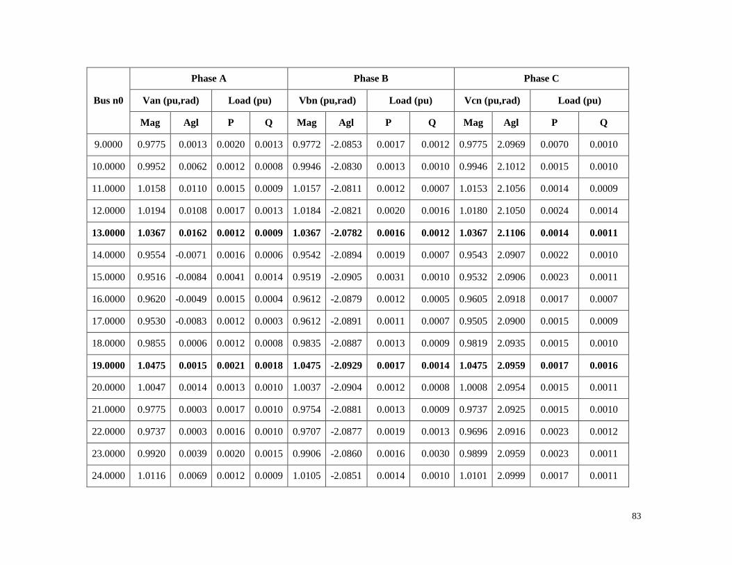
83
Bus n0
Phase A Phase B Phase C
Van (pu,rad) Load (pu) Vbn (pu,rad) Load (pu) Vcn (pu,rad) Load (pu)
Mag Agl P Q Mag Agl P Q Mag Agl P Q
9.0000 0.9775 0.0013 0.0020 0.0013 0.9772 -2.0853 0.0017 0.0012 0.9775 2.0969 0.0070 0.0010
10.0000 0.9952 0.0062 0.0012 0.0008 0.9946 -2.0830 0.0013 0.0010 0.9946 2.1012 0.0015 0.0010
11.0000 1.0158 0.0110 0.0015 0.0009 1.0157 -2.0811 0.0012 0.0007 1.0153 2.1056 0.0014 0.0009
12.0000 1.0194 0.0108 0.0017 0.0013 1.0184 -2.0821 0.0020 0.0016 1.0180 2.1050 0.0024 0.0014
13.0000 1.0367 0.0162 0.0012 0.0009 1.0367 -2.0782 0.0016 0.0012 1.0367 2.1106 0.0014 0.0011
14.0000 0.9554 -0.0071 0.0016 0.0006 0.9542 -2.0894 0.0019 0.0007 0.9543 2.0907 0.0022 0.0010
15.0000 0.9516 -0.0084 0.0041 0.0014 0.9519 -2.0905 0.0031 0.0010 0.9532 2.0906 0.0023 0.0011
16.0000 0.9620 -0.0049 0.0015 0.0004 0.9612 -2.0879 0.0012 0.0005 0.9605 2.0918 0.0017 0.0007
17.0000 0.9530 -0.0083 0.0012 0.0003 0.9612 -2.0891 0.0011 0.0007 0.9505 2.0900 0.0015 0.0009
18.0000 0.9855 0.0006 0.0012 0.0008 0.9835 -2.0887 0.0013 0.0009 0.9819 2.0935 0.0015 0.0010
19.0000 1.0475 0.0015 0.0021 0.0018 1.0475 -2.0929 0.0017 0.0014 1.0475 2.0959 0.0017 0.0016
20.0000 1.0047 0.0014 0.0013 0.0010 1.0037 -2.0904 0.0012 0.0008 1.0008 2.0954 0.0015 0.0011
21.0000 0.9775 0.0003 0.0017 0.0010 0.9754 -2.0881 0.0013 0.0009 0.9737 2.0925 0.0015 0.0010
22.0000 0.9737 0.0003 0.0016 0.0010 0.9707 -2.0877 0.0019 0.0013 0.9696 2.0916 0.0023 0.0012
23.0000 0.9920 0.0039 0.0020 0.0015 0.9906 -2.0860 0.0016 0.0030 0.9899 2.0959 0.0023 0.0011
24.0000 1.0116 0.0069 0.0012 0.0009 1.0105 -2.0851 0.0014 0.0010 1.0101 2.0999 0.0017 0.0011

84
Bus n0
Phase A Phase B Phase C
Van (pu,rad) Load (pu) Vbn (pu,rad) Load (pu) Vcn (pu,rad) Load (pu)
Mag Agl P Q Mag Agl P Q Mag Agl P Q
25.0000 1.0341 0.0097 0.0021 0.0017 1.0341 -2.0847 0.0017 0.0011 1.0341 2.1041 0.0014 0.0013
Total PLa QLa PLb QLb PLc QLc PLtotal QLtotal f/pu Ploss Vmin/pu Vmax/pu
0.0357 0.0212 0.0346 0.0223 0.0377 0.0377 0.1080 0.0812 0.9997 0.0055 0.0975 1.0475
TABLE XVIII. DG UNITS REAL AND REACTIVE POWER GENERATION IN 25-BUS UNBALANCED TEST SYSTEM, KG13=15 AND KG19=15
Busid(DG) PGa PGb PGc QGa QGb QGc
13 0.0110 0.1110 0.0119 0.0049 0.0054 0.0060
19 0.0114 0.0101 0.0118 0.0081 0.0083 0.0084
25 0.0150 0.0145 0.0159 0.0094 0.0097 0.0101
TABLE XIX. VOLTAGE PROFILE AND LOADS RESULTS OF THE PROPOSED POWER FLOW IN 25-BUS UNBALANCED
TEST SYSTEM, KG13=15 AND KG19=20
Bus n0
Phase A Phase B Phase C
Van (pu,rad) Load (pu) Vbn (pu,rad) Load (pu) Vcn (pu,rad) Load (pu)
Mag Agl P Q Mag Agl P Q Mag Agl P Q
1 0.9763 -0.0000 0.0000 0.0000 0.9742 -2.0879 0.0000 0.0000 0.9733 2.0922 0.0000 0.0000
2 0.9763 0.0000 0.0000 0.0000 0.9742 -2.0879 0.0000 0.0000 0.9733 2.0922 0.0000 0.0000
3 0.9768 0.0005 0.0012 0.0007 0.9747 -2.0875 0.0013 0.0009 0.9737 2.0925 0.0015 0.0009

85
Bus n0
Phase A Phase B Phase C
Van (pu,rad) Load (pu) Vbn (pu,rad) Load (pu) Vcn (pu,rad) Load (pu)
Mag Agl P Q Mag Agl P Q Mag Agl P Q
4 0.9771 0.0007 0.0016 0.0012 0.9750 -2.0875 0.0019 0.0014 0.9740 2.0925 0.0022 0.0011
5 0.9734 0.0022 0.0013 0.0009 0.9711 -2.0858 0.0012 0.0008 0.9695 2.0932 0.0016 0.0009
6 0.9648 -0.0069 0.0013 0.0005 0.9631 -2.0919 0.0015 0.0009 0.9636 2.0883 0.0012 0.0007
7 0.9644 -0.0096 0.0000 0.0000 0.9636 -2.0939 0.0000 0.0000 0.9634 2.0864 0.0000 0.0000
8 0.9567 -0.0104 0.0011 0.0003 0.9554 -2.0935 0.0014 0.0009 0.9566 2.0867 0.0012 0.0008
9 0.9768 -0.0081 0.0020 0.0013 0.9766 -2.0948 0.0017 0.0012 0.9767 2.0872 0.0017 0.0010
10 0.9944 0.0064 0.0012 0.0008 0.9940 -2.0957 0.0013 0.0010 0.9938 2.0884 0.0015 0.0010
11 1.0150 -0.0048 0.0015 0.0009 1.0149 -2.0968 0.0012 0.0007 1.0145 2.0898 0.0014 0.0009
12 1.0185 -0.0046 0.0017 0.0013 1.0176 -2.0975 0.0020 0.0016 1.0171 2.0895 0.0024 0.0014
13 1.0359 -0.0029 0.0012 0.0009 1.0359 -2.0973 0.0016 0.0012 1.0359 2.0915 0.0014 0.0011
14 0.9547 -0.0125 0.0016 0.0006 0.9538 -2.0949 0.0019 0.0007 0.9536 2.0849 0.0022 0.0010
15 0.9509 -0.0132 0.0041 0.0014 0.9514 -2.0953 0.0031 0.0010 0.9525 2.0854 0.0023 0.0011
16 0.9614 -0.0110 0.0015 0.0004 0.9608 -2.0941 0.0012 0.0005 0.9597 2.0853 0.0017 0.0007
17 0.9523 -0.0137 0.0012 0.0003 0.9508 -2.0946 0.0011 0.0007 0.9498 2.0842 0.0015 0.0009
18 0.9851 0.0075 0.0012 0.0008 0.9835 -2.0820 0.0013 0.0009 0.9811 2.0996 0.0015 0.0010
19 1.0484 0.0309 0.0021 0.0018 1.0484 -2.0635 0.0017 0.0014 1.0484 2.1253 0.0017 0.0016

86
Bus n0
Phase A Phase B Phase C
Van (pu,rad) Load (pu) Vbn (pu,rad) Load (pu) Vcn (pu,rad) Load (pu)
Mag Agl P Q Mag Agl P Q Mag Agl P Q
20 1.0044 0.0164 0.0013 0.0010 1.0041 -2.0756 0.0012 0.0008 1.0002 2.1094 0.0015 0.0011
21 0.9770 0.0054 0.0017 0.0010 0.9753 -2.0830 0.0013 0.0009 0.9731 2.0969 0.0015 0.0010
22 0.9731 0.0038 0.0016 0.0010 0.9705 -2.0843 0.0019 0.0013 0.9688 2.0944 0.0023 0.0012
23 0.9913 -0.0012 0.0020 0.0015 0.9901 -2.0912 0.0016 0.0013 0.9891 2.0905 0.0023 0.0011
24 1.0107 -0.0030 0.0012 0.0009 1.0098 -2.0951 0.0014 0.0010 1.0092 2.0898 0.0017 0.0011
25 1.0332 -0.0049 0.0021 0.0017 1.0332 -2.0993 0.0017 0.0011 1.0332 2.0895 0.0014 13.0000
Total PLa QLa PLb QLb PLc QLc PLtotal QLtotal f/pu Ploss Vmin/pu Vmax/pu
0.0357 0.0212 0.0346 0.0223 0.0377 0.0377 0.1080 0.0811 0.9999 0.0058 0.9498 1.0484
TABLE XX. DG UNITS REAL AND REACTIVE POWER GENERATION IN 25-BUS UNBALANCED TEST SYSTEM, KG13=15
AND KG19=20
Busid(DG) PGa PGb PGc QGa QGb QGc
13 0.0100 0.0102 0.0108 0.0062 0.0068 0.0074
19 0.0138 0.0131 0.0144 0.0052 0.0052 0.0053
25 0.0136 0.0132 0.0145 0.0111 0.0114 0.0117

87
TABLE XXI. VOLTAGE PROFILE AND LOADS RESULTS OF THE PROPOSED POWER FLOW IN 25-BUS UNBALANCED
TEST SYSTEM, KG13=17 AND KG19=20
Bus n0
Phase A Phase B Phase C
Van (pu,rad) Load (pu) Vbn (pu,rad) Load (pu) Vcn (pu,rad) Load (pu)
Mag Agl P Q Mag Agl P Q Mag Agl P Q
1 0.9763 0.0000 0.0000 0.0000 0.9742 -2.0879 0.0000 0.0000 0.9734 2.0923 0.0000 0.0000
2 0.9763 0.0000 0.0000 0.0000 0.9742 -2.0879 0.0000 0.0000 0.9734 2.0923 0.0000 0.0000
3 0.9768 0.0005 0.0012 0.0007 0.9747 -2.0876 0.0013 0.0009 0.9738 2.0926 0.0015 0.0009
4 0.9771 0.0006 0.0016 0.0012 0.9749 -2.0876 0.0019 0.0014 0.9741 2.0926 0.0022 0.0011
5 0.9734 0.0017 0.0013 0.0009 0.9711 -2.0862 0.0012 0.0008 0.9696 2.0929 0.0016 0.0009
6 0.9649 -0.0056 0.0013 0.0005 0.9632 -2.0905 0.0015 0.0009 0.9637 2.0897 0.0012 0.0007
7 0.9646 -0.0073 0.0000 0.0000 0.9637 -2.0915 0.0000 0.0000 0.9636 2.0889 0.0000 0.0000
8 0.9568 -0.0089 0.0011 0.0003 0.9554 -2.0920 0.0014 0.0009 0.9567 2.0883 0.0012 0.0008
9 0.9770 -0.0045 0.0020 0.0013 0.9768 -2.0911 0.0017 0.0012 0.9769 2.0910 0.0017 0.0010
10 0.9947 -0.0015 0.0012 0.0008 0.9942 -2.0908 0.0013 0.0010 0.9941 2.0934 0.0015 0.0010
11 1.0154 0.0013 0.0015 0.0009 1.0152 -2.0907 0.0012 0.0007 1.0149 2.0960 0.0014 0.0009
12 1.0187 -0.0002 0.0017 0.0013 1.0177 -2.0930 0.0020 0.0016 1.0173 2.0941 0.0024 0.0014
13 1.0366 0.0061 0.0012 0.0009 1.0366 -2.0883 0.0016 0.0012 1.0366 2.1005 0.0014 0.0011
14 0.9548 -0.0104 0.0016 0.0006 0.9538 -2.0928 0.0019 0.0007 0.9537 2.0871 0.0022 0.0010
15 0.9510 -0.0113 0.0041 0.0014 0.9515 -2.0934 0.0031 0.0010 0.9526 2.0874 0.0023 0.0011

88
Bus n0
Phase A Phase B Phase C
Van (pu,rad) Load (pu) Vbn (pu,rad) Load (pu) Vcn (pu,rad) Load (pu)
Mag Agl P Q Mag Agl P Q Mag Agl P Q
16 0.9615 -0.0086 0.0015 0.0004 0.9609 -2.0917 0.0012 0.0005 0.9599 2.0878 0.0017 0.0007
17 0.9525 -0.0116 0.0012 0.0003 0.9509 -2.0925 0.0011 0.0007 0.9499 2.0864 0.0015 0.0009
18 0.9851 0.0061 0.0012 0.0008 0.9834 -2.0834 0.0013 0.0009 0.9812 2.0983 0.0015 0.0010
19 1.0482 0.0249 0.0021 0.0018 1.0482 -2.0695 0.0017 0.0014 1.0482 2.1193 0.0017 0.0016
20 1.0044 0.0133 0.0013 0.0010 1.0040 -2.0787 0.0012 0.0008 1.0003 2.1066 0.0015 0.0011
21 0.9770 0.0043 0.0017 0.0010 0.9752 -2.0841 0.0013 0.0009 0.9732 2.0960 0.0015 0.0010
22 0.9732 0.0030 0.0016 0.0010 0.9705 -2.0851 0.0019 0.0013 0.9689 2.0938 0.0023 0.0012
23 0.9912 -0.0008 0.0020 0.0015 0.9900 -2.0908 0.0016 0.0013 0.9890 2.0910 0.0023 0.0011
24 1.0106 -0.0022 0.0012 0.0009 1.0096 -2.0943 0.0014 0.0010 1.0090 2.0906 0.0017 0.0011
25 1.0329 -0.0037 0.0021 0.0017 1.0329 -2.0981 0.0017 0.0011 1.0329 2.0907 0.0014 0.0013
Total PLa QLa PLb QLb PLc QLc PLtotal QLtotal f/pu Ploss Vmin/pu Vmax/pu
0.0357 0.0212 0.0346 0.0223 0.0377 0.0377 0.1080 0.0811 1.0000 0.0057 0.9499 1.0482

89
TABLE XXII. DG UNITS REAL AND REACTIVE POWER GENERATION IN 25-BUS UNBALANCED TEST SYSTEM, KG13=17 AND KG19=20
Busid(DG) PGa PGb PGc QGa QGb QGc
13 0.0110 0.0111 0.0118 0.0052 0.0057 0.0063
19 0.0133 0.0126 0.0139 0.0058 0.0059 0.0060
25 0.0132 0.0128 0.0140 0.0115 0.0119 0.0122
TABLE XXIII. VOLTAGE PROFILE AND LOADS RESULTS OF THE PROPOSED POWER FLOW IN 25-BUS UNBALANCED
TEST SYSTEM, KG13=10 AND F025=1.003
Bus n0
Phase A Phase B Phase C
Van (pu,rad) Load (pu) Vbn (pu,rad) Load (pu) Vcn (pu,rad) Load (pu)
Mag Agl P Q Mag Agl P Q Mag Agl P Q
1 0.9777 0.0000 0.0000 0.0000 0.9750 -2.0877 0.0000 0.0000 0.9752 2.0934 0.0000 0.0000
2 0.9777 0.0000 0.0000 0.0000 0.9750 -2.0877 0.0000 0.0000 0.9752 2.0934 0.0000 0.0000
3 0.9782 0.0003 0.0012 0.0007 0.9755 -2.0875 0.0013 0.0009 0.9757 2.0936 0.0015 0.0009
4 0.9784 0.0011 0.0016 0.0012 0.9757 -2.0869 0.0019 0.0014 0.9758 2.0942 0.0022 0.0011
5 0.9746 -0.0017 0.0013 0.0009 0.9716 -2.0895 0.0012 0.0008 0.9712 2.0907 0.0016 0.0009
6 0.9660 -0.0026 0.0013 0.0005 0.9639 -2.0874 0.0015 0.0009 0.9651 2.0935 0.0012 0.0007
7 0.9654 -0.0019 0.0000 0.0000 0.9642 -2.0861 0.0000 0.0000 0.9646 2.0948 0.0000 0.0000
8 0.9579 -0.0053 0.0011 0.0003 0.9561 -2.0883 0.0014 0.0009 0.9580 2.0927 0.0012 0.0008

90
Bus n0
Phase A Phase B Phase C
Van (pu,rad) Load (pu) Vbn (pu,rad) Load (pu) Vcn (pu,rad) Load (pu)
Mag Agl P Q Mag Agl P Q Mag Agl P Q
9 0.9776 0.0038 0.0020 0.0013 0.9772 -2.0828 0.0017 0.0012 0.9775 2.0995 0.0017 0.0010
10 0.9950 0.0096 0.0012 0.0008 0.9945 -2.0797 0.0013 0.0010 0.9944 2.1044 0.0015 0.0010
11 1.0154 0.0151 0.0015 0.0009 1.0154 -2.0770 0.0012 0.0007 1.0148 2.1094 0.0014 0.0009
12 1.0204 0.0253 0.0017 0.0013 1.0199 -2.0679 0.0020 0.0016 1.0185 2.1186 0.0024 0.0014
13 1.0347 0.0110 0.0012 0.0009 1.0347 -2.0834 0.0016 0.0012 1.0347 2.1054 0.0014 0.0011
14 0.9557 -0.0057 0.0016 0.0006 0.9544 -2.0879 0.0019 0.0007 0.9548 2.0925 0.0022 0.0010
15 0.9520 -0.0072 0.0041 0.0014 0.9521 -2.0892 0.0031 0.0010 0.9538 2.0922 0.0023 0.0011
16 0.9624 -0.0033 0.0015 0.0004 0.9614 -2.0863 0.0012 0.0005 0.9609 2.0937 0.0017 0.0007
17 0.9533 -0.0069 0.0012 0.0003 0.9515 -2.0876 0.0011 0.0007 0.9510 2.0918 0.0015 0.0009
18 0.9859 -0.0092 0.0012 0.0008 0.9833 -2.0983 0.0013 0.0009 0.9827 2.0846 0.0015 0.0010
19 1.0462 -0.0417 0.0021 0.0018 1.0462 -2.1361 0.0017 0.0014 1.0462 2.0527 0.0017 0.0016
20 1.0045 -0.0206 0.0013 0.0010 1.0027 -2.1121 0.0012 0.0008 1.0013 2.0748 0.0015 0.0011
21 0.9779 -0.0070 0.0017 0.0010 0.9753 -2.0952 0.0013 0.0009 0.9747 2.0861 0.0015 0.0010
22 0.9742 -0.0044 0.0016 0.0011 0.9708 -2.0922 0.0019 0.0013 0.9705 2.0878 0.0023 0.0012
23 0.9938 0.0157 0.0020 0.0015 0.9922 -2.0741 0.0016 0.0013 0.9919 2.1082 0.0023 0.0011
24 1.0146 0.0297 0.0012 0.0009 1.0135 -2.0623 0.0014 0.0010 1.0132 2.1229 0.0017 0.0011

91
Bus n0
Phase A Phase B Phase C
Van (pu,rad) Load (pu) Vbn (pu,rad) Load (pu) Vcn (pu,rad) Load (pu)
Mag Agl P Q Mag Agl P Q Mag Agl P Q
25 1.0386 0.0430 0.0021 0.0017 1.0386 -2.0514 0.0018 0.0011 1.0386 2.1374 0.0014 0.0013
Total PLa QLa PLb QLb PLc QLc PLtotal QLtotal f/pu Ploss Vmin/pu Vmax/pu
0.0357 0.0213 0.0347 0.0223 0.0377 0.0377 0.1081 0.0813 0.9996 0.0072 0.9510 1.0462
TABLE XXIV. DG UNITS REAL AND REACTIVE POWER GENERATION IN 25-BUS UNBALANCED TEST SYSTEM, KG13=10 AND F025=1.003
Busid(DG) PGa PGb PGc QGa QGb QGc
13 0.0077 0.0079 0.0083 0.0082 0.0089 0.0094
19 0.0080 0.0076 0.0081 0.0126 0.0129 0.0130
25 0.0223 0.0216 0.0238 0.0022 0.0021 0.0026
TABLE XXV. VOLTAGE PROFILE AND LOADS RESULTS OF THE PROPOSED POWER FLOW IN 25-BUS UNBALANCED
TEST SYSTEM, KG13=18 AND F025=1.003
Bus n0
Phase A Phase B Phase C
Van (pu,rad) Load (pu) Vbn (pu,rad) Load (pu) Vcn (pu,rad) Load (pu)
Mag Agl P Q Mag Agl P Q Mag Agl P Q
1 0.9768 0.0000 0.0000 0.0000 0.9739 -2.0876 0.0000 0.0000 0.9745 2.0938 0.0000 0.0000

92
Bus n0
Phase A Phase B Phase C
Van (pu,rad) Load (pu) Vbn (pu,rad) Load (pu) Vcn (pu,rad) Load (pu)
Mag Agl P Q Mag Agl P Q Mag Agl P Q
2 0.9768 0.0000 0.0000 0.0000 0.9739 -2.0876 0.0000 0.0000 0.9745 2.0938 0.0000 0.0000
3 0.9774 0.0001 0.0012 0.0007 0.9745 -2.0877 0.0013 0.0009 0.9750 2.0938 0.0015 0.0009
4 0.9776 0.0008 0.0016 0.0012 0.9746 -2.0871 0.0019 0.0014 0.9751 2.0943 0.0022 0.0011
5 0.9738 -0.0031 0.0013 0.0009 0.9705 -2.0907 0.0012 0.0008 0.9705 2.0898 0.0016 0.0009
6 0.9654 0.0022 0.0013 0.0005 0.9631 -2.0825 0.0015 0.0009 0.9647 2.0988 0.0012 0.0007
7 0.9652 0.0069 0.0000 0.0000 0.9639 -2.0772 0.0000 0.0000 0.9645 2.1040 0.0000 0.0000
8 0.9574 0.0005 0.0011 0.0003 0.9554 -2.0823 0.0014 0.0009 0.9577 2.0989 0.0012 0.0008
9 0.9778 0.0175 0.0020 0.0013 0.9773 -2.0690 0.0017 0.0012 0.9779 2.1136 0.0017 0.0010
10 0.9957 0.0280 0.0012 0.0008 0.9951 -2.0612 0.0013 0.0010 0.9953 2.1232 0.0015 0.0010
11 1.0168 0.0381 0.0015 0.0009 1.0166 -2.0539 0.0012 0.0007 1.0162 2.1328 0.0014 0.0009
12 1.0209 0.0406 0.0017 0.0013 1.0201 -2.0523 0.0020 0.0016 1.0194 2.1347 0.0024 0.0014
13 1.0374 0.0458 0.0012 0.0009 1.0374 -2.0485 0.0016 0.0012 1.0374 2.1402 0.0014 0.0011
14 0.9555 0.0022 0.0016 0.0006 0.9540 -2.0800 0.0019 0.0007 0.9547 2.1007 0.0022 0.0010
15 0.9516 -0.0003 0.0041 0.0014 0.9516 -2.0822 0.0031 0.0010 0.9536 2.0995 0.0023 0.0011
16 0.9622 0.0056 0.0015 0.0004 0.9611 -2.0774 0.0012 0.0005 0.9608 2.1029 0.0017 0.0007
17 0.9531 0.0010 0.0012 0.0003 0.9510 -2.0797 0.0011 0.0007 0.9509 2.1000 0.0015 0.0009

93
Bus n0
Phase A Phase B Phase C
Van (pu,rad) Load (pu) Vbn (pu,rad) Load (pu) Vcn (pu,rad) Load (pu)
Mag Agl P Q Mag Agl P Q Mag Agl P Q
18 0.9850 -0.0137 0.0012 0.0008 0.9821 -2.1028 0.0013 0.0009 0.9820 2.0806 0.0015 0.0010
19 1.0455 -0.0605 0.0021 0.0018 1.0455 -2.1549 0.0017 0.0014 1.0455 2.0339 0.0017 0.0016
20 1.0037 -0.0303 0.0013 0.0010 1.0015 -2.1217 0.0012 0.0008 1.0007 2.0658 0.0015 0.0011
21 0.9771 -0.0105 0.0017 0.0010 0.9741 -2.0986 0.0013 0.0009 0.9740 2.0831 0.0015 0.0010
22 0.9733 -0.0068 0.0016 0.0010 0.9696 -2.0946 0.0019 0.0013 0.9698 2.0858 0.0023 0.0012
23 0.9927 0.0160 0.0020 0.0015 0.9910 -2.0738 0.0016 0.0013 0.9909 2.1088 0.0023 0.0011
24 1.0133 0.0306 0.0012 0.0009 1.0122 -2.0614 0.0014 0.0010 1.0119 2.1239 0.0017 0.0011
25 1.0371 0.0445 0.0021 0.0017 1.0371 -2.0499 0.0018 0.0011 1.0371 2.1389 0.0014 0.0013
Total PLa QLa PLb QLb PLc QLc PLtotal QLtotal f/pu Ploss Vmin/pu Vmax/pu
0.0357 0.0212 0.0346 0.0223 0.0377 0.0377 0.1081 0.0812 1.0000 0.0079 0.9509 1.0455
TABLE XXVI. DG UNITS REAL AND REACTIVE POWER GENERATION IN 25-BUS UNBALANCED TEST SYSTEM, KG13=18 AND F025=1.003
Busid(DG) PGa PGb PGc QGa QGb QGc
13 0.0117 0.0117 0.0126 0.0039 0.0043 0.0049
19 0.0068 0.0064 0.0068 0.0146 0.0150 0.0151
25 0.0198 0.0192 0.0211 0.0046 0.0047 0.0051

94
TABLE XXVII. VOLTAGE PROFILE AND LOADS RESULTS OF THE PROPOSED POWER FLOW IN 25-BUS UNBALANCED
TEST SYSTEM, KG13=10 AND F025=1.0035
Bus n0
Phase A Phase B Phase C
Van (pu,rad) Load (pu) Vbn (pu,rad) Load (pu) Vcn (pu,rad) Load (pu)
Mag Agl P Q Mag Agl P Q Mag Agl P Q
1 0.9777 0.0000 0.0000 0.0000 0.9749 -2.0876 0.0000 0.0000 0.9753 2.0936 0.0000 0.0000
2 0.9777 0.0000 0.0000 0.0000 0.9749 -2.0876 0.0000 0.0000 0.9753 2.0936 0.0000 0.0000
3 0.9783 0.0003 0.0012 0.0007 0.9754 -2.0875 0.0013 0.0009 0.9757 2.0937 0.0015 0.0009
4 0.9784 0.0012 0.0016 0.0012 0.9756 -2.0868 0.0019 0.0014 0.9758 2.0944 0.0022 0.0011
5 0.9745 -0.0022 0.0013 0.0009 0.9715 -2.0899 0.0012 0.0008 0.9712 2.0903 0.0016 0.0009
6 0.9659 -0.0024 0.0013 0.0005 0.9638 -2.0872 0.0015 0.0009 0.9651 2.0938 0.0012 0.0007
7 0.9653 -0.0015 0.0000 0.0000 0.9641 -2.0857 0.0000 0.0000 0.9645 2.0953 0.0000 0.0000
8 0.9578 -0.0050 0.0011 0.0003 0.9560 -2.0880 0.0014 0.0009 0.9580 2.0930 0.0012 0.0008
9 0.9774 0.0044 0.0020 0.0013 0.9771 -2.0822 0.0017 0.0012 0.9775 2.1001 0.0017 0.0010
10 0.9949 0.0104 0.0012 0.0008 0.9944 -2.0788 0.0013 0.0010 0.9942 2.1052 0.0015 0.0010
11 1.0153 0.0162 0.0015 0.0009 1.0153 -2.0759 0.0012 0.0007 1.0145 2.1104 0.0014 0.0009
12 1.0205 0.0288 0.0017 0.0013 1.0201 -2.0644 0.0020 0.0016 1.0185 2.1219 0.0024 0.0014
13 1.0342 0.0099 0.0012 0.0009 1.0342 -2.0845 0.0016 0.0012 1.0342 2.1043 0.0014 0.0011
14 0.9557 -0.0053 0.0016 0.0006 0.9543 -2.0875 0.0019 0.0007 0.9548 2.0929 0.0022 0.0010
15 0.9519 -0.0069 0.0041 0.0014 0.9520 -2.0888 0.0031 0.0010 0.9538 2.0927 0.0023 0.0011

95
Bus n0
Phase A Phase B Phase C
Van (pu,rad) Load (pu) Vbn (pu,rad) Load (pu) Vcn (pu,rad) Load (pu)
Mag Agl P Q Mag Agl P Q Mag Agl P Q
16 0.9623 -0.0029 0.0015 0.0004 0.9613 -2.0859 0.0012 0.0005 0.9609 2.0942 0.0017 0.0007
17 0.9533 -0.0065 0.0012 0.0003 0.9514 -2.0872 0.0011 0.0007 0.9510 2.0922 0.0015 0.0009
18 0.9858 -0.0116 0.0012 0.0008 0.9830 -2.1007 0.0013 0.0009 0.9827 2.0825 0.0015 0.0010
19 1.0458 -0.0520 0.0021 0.0018 1.0458 -2.1464 0.0017 0.0014 1.0458 2.0424 0.0017 0.0016
20 1.0043 -0.0258 0.0013 0.0010 1.0023 -2.1172 0.0012 0.0008 1.0012 2.0699 0.0015 0.0011
21 0.9778 -0.0088 0.0017 0.0010 0.9751 -2.0969 0.0013 0.0009 0.9747 2.0845 0.0015 0.0010
22 0.9741 -0.0055 0.0016 0.0010 0.9706 -2.0933 0.0019 0.0013 0.9705 2.0868 0.0023 0.0012
23 0.9940 0.0185 0.0020 0.0015 0.9924 -2.0713 0.0016 0.0013 0.9922 2.1111 0.0023 0.0011
24 1.0152 0.0351 0.0012 0.0009 1.0141 -2.0569 0.0014 0.0010 1.0138 2.1283 0.0017 0.0011
25 1.0397 0.0509 0.0021 0.0017 1.0397 -2.0435 0.0018 0.0011 1.0397 2.1453 0.0014 0.0013
Total PLa QLa PLb QLb PLc QLc PLtotal QLtotal f/pu Ploss Vmin/pu Vmax/pu
0.0357 0.0213 0.0347 0.0223 0.0377 0.0377 0.1081 0.0813 0.9998 0.0080 0.9510 1.0458

96
TABLE XXVIII. DG UNITS REAL AND REACTIVE POWER GENERATION IN 25-BUS UNBALANCED TEST SYSTEM, KG13=10 AND F025=1.0035
Busid(DG) PGa PGb PGc QGa QGb QGc
13 0.0069 0.0071 0.0074 0.0089 0.0097 0.0102
19 0.0073 0.0069 0.0073 0.0136 0.0141 0.0141
25 0.0241 0.0233 0.0257 0.0005 0.0003 0.0008
TABLE XXIX. VOLTAGE PROFILE AND LOADS RESULTS OF THE PROPOSED POWER FLOW IN 25-BUS UNBALANCED
TEST SYSTEM, KG13=13 AND F025=1.0035
Bus n0
Phase A Phase B Phase C
Van (pu,rad) Load (pu) Vbn (pu,rad) Load (pu) Vcn (pu,rad) Load (pu)
Mag Agl P Q Mag Agl P Q Mag Agl P Q
1 0.9774 0.0000 0.0000 0.0000 0.9745 -2.0876 0.0000 0.0000 0.9750 2.0937 0.0000 0.0000
2 0.9774 0.0000 0.0000 0.0000 0.9745 -2.0876 0.0000 0.0000 0.9750 2.0937 0.0000 0.0000
3 0.9780 0.0002 0.0012 0.0007 0.9751 -2.0875 0.0013 0.0009 0.9755 2.0938 0.0015 0.0009
4 0.9781 0.0011 0.0016 0.0012 0.9752 -2.0868 0.0019 0.0014 0.9756 2.0945 0.0022 0.0011
5 0.9742 -0.0027 0.0013 0.0009 0.9710 -2.0904 0.0012 0.0008 0.9710 2.0900 0.0016 0.0009
6 0.9658 -0.0005 0.0013 0.0005 0.9635 -2.0853 0.0015 0.0009 0.9650 2.0958 0.0012 0.0007
7 0.9653 0.0019 0.0000 0.0000 0.9640 -2.0823 0.0000 0.0000 0.9646 2.0988 0.0000 0.0000
8 0.9577 -0.0028 0.0011 0.0003 0.9558 -2.0857 0.0014 0.0009 0.9579 2.0954 0.0012 0.0008

97
Bus n0
Phase A Phase B Phase C
Van (pu,rad) Load (pu) Vbn (pu,rad) Load (pu) Vcn (pu,rad) Load (pu)
Mag Agl P Q Mag Agl P Q Mag Agl P Q
9 0.9776 0.0097 0.0020 0.0013 0.9772 -2.0769 0.0017 0.0012 0.9777 2.1055 0.0017 0.0010
10 0.9952 0.0175 0.0012 0.0008 0.9947 -2.0718 0.0013 0.0010 0.9946 2.1124 0.0015 0.0010
11 1.0158 0.0250 0.0015 0.0009 1.0158 -2.0671 0.0012 0.0007 1.0152 2.1194 0.0014 0.0009
12 1.0208 0.0347 0.0017 0.0013 1.0203 -2.0585 0.0020 0.0016 1.0190 2.1281 0.0024 0.0014
13 1.0353 0.0233 0.0012 0.0009 1.0353 -2.0711 0.0016 0.0012 1.0353 2.1177 0.0014 0.0011
14 0.9556 -0.0023 0.0016 0.0006 0.9542 -2.0845 0.0019 0.0007 0.9548 2.0961 0.0022 0.0010
15 0.9518 -0.0043 0.0041 0.0014 0.9518 -2.0862 0.0031 0.0010 0.9538 2.0954 0.0023 0.0011
16 0.9623 0.0005 0.0015 0.0004 0.9612 -2.0824 0.0012 0.0005 0.9609 2.0977 0.0017 0.0007
17 0.9532 -0.0035 0.0012 0.0003 0.9512 -2.0842 0.0011 0.0007 0.9510 2.0954 0.0015 0.0009
18 0.9854 -0.0133 0.0012 0.0008 0.9826 -2.1024 0.0013 0.0009 0.9824 2.0809 0.0015 0.0010
19 1.0456 -0.0593 0.0021 0.0018 1.0456 -2.1537 0.0017 0.0014 1.0456 2.0351 0.0017 0.0016
20 1.0040 -0.0295 0.0013 0.0010 1.0018 -2.1210 0.0012 0.0008 1.0010 2.0664 0.0015 0.0011
21 0.9775 -0.0101 0.0017 0.0010 0.9746 -2.0982 0.0013 0.0009 0.9745 2.0834 0.0015 0.0010
22 0.9738 -0.0065 0.0016 0.0010 0.9701 -2.0942 0.0019 0.0013 0.9702 2.0861 0.0023 0.0012
23 0.9936 0.0186 0.0020 0.0015 0.9920 -2.0711 0.0016 0.0013 0.9918 2.1114 0.0023 0.0011
24 1.0147 0.0355 0.0012 0.0009 1.0136 -2.0565 0.0014 0.0010 1.0133 2.1288 0.0017 0.0011

98
Bus n0
Phase A Phase B Phase C
Van (pu,rad) Load (pu) Vbn (pu,rad) Load (pu) Vcn (pu,rad) Load (pu)
Mag Agl P Q Mag Agl P Q Mag Agl P Q
25 1.0391 0.0515 0.0021 0.0017 1.0391 -2.0429 0.0018 0.0011 1.0391 2.1459 0.0014 0.0013
Total PLa QLa PLb QLb PLc QLc PLtotal QLtotal f/pu Ploss Vmin/pu Vmax/pu
0.0357 0.0213 0.0347 0.0223 0.0377 0.0377 0.1081 0.0813 1.0000 0.0082 0.9510 1.0456
TABLE XXX. DG UNITS REAL AND REACTIVE POWER GENERATION IN 25-BUS UNBALANCED TEST SYSTEM, KG13=13 AND F025=1.0035
Busid(DG) PGa PGb PGc QGa QGb QGc
13 0.0084 0.0086 0.0091 0.0073 0.0079 0.0084
19 0.0068 0.0065 0.0068 0.0144 0.0149 0.0150
25 0.0231 0.0224 0.0246 0.0014 0.0013 0.0018
TABLE XXXI. VOLTAGE PROFILE AND LOADS RESULTS OF THE PROPOSED POWER FLOW IN 25-BUS UNBALANCED
TEST SYSTEM, KG19=15 AND F025=1.003
Bus n0
Phase A Phase B Phase C
Van (pu,rad) Load (pu) Vbn (pu,rad) Load (pu) Vcn (pu,rad) Load (pu)
Mag Agl P Q Mag Agl P Q Mag Agl P Q
1 0.9778 0.0000 0.0000 0.0000 0.9754 -2.0878 0.0000 0.0000 0.9750 2.0928 0.0000 0.0000

99
Bus n0
Phase A Phase B Phase C
Van (pu,rad) Load (pu) Vbn (pu,rad) Load (pu) Vcn (pu,rad) Load (pu)
Mag Agl P Q Mag Agl P Q Mag Agl P Q
2 0.9778 0.0000 0.0000 0.0000 0.9754 -2.0878 0.0000 0.0000 0.9750 2.0928 0.0000 0.0000
3 0.9782 0.0005 0.0012 0.0007 0.9759 -2.0874 0.0013 0.0009 0.9754 2.0931 0.0015 0.0009
4 0.9784 0.0011 0.0016 0.0012 0.9761 -2.0870 0.0019 0.0014 0.9756 2.0935 0.0022 0.0011
5 0.9747 0.0002 0.0013 0.0009 0.9721 -2.0877 0.0012 0.0008 0.9711 2.0919 0.0016 0.0009
6 0.9658 -0.0062 0.0013 0.0005 0.9640 -2.0912 0.0015 0.0009 0.9648 2.0894 0.0012 0.0007
7 0.9652 -0.0085 0.0000 0.0000 0.9642 -2.0927 0.0000 0.0000 0.9642 2.0878 0.0000 0.0000
8 0.9577 -0.0096 0.0011 0.0003 0.9562 -2.0927 0.0014 0.0009 0.9577 2.0878 0.0012 0.0008
9 0.9772 -0.0064 0.0020 0.0013 0.9770 -2.0930 0.0017 0.0012 0.9771 2.0890 0.0017 0.0010
10 0.9945 -0.0041 0.0012 0.0008 0.9941 -2.0934 0.0013 0.0010 0.9937 2.0906 0.0015 0.0010
11 1.0147 -0.0019 0.0015 0.0009 1.0147 -2.0940 0.0012 0.0007 1.0140 2.0923 0.0014 0.0009
12 1.0195 0.0082 0.0017 0.0013 1.0190 -2.0849 0.0020 0.0016 1.0176 2.1015 0.0024 0.0014
13 1.0339 -0.0092 0.0012 0.0009 1.0339 -2.1036 0.0016 0.0012 1.0339 2.0852 0.0014 0.0011
14 0.9556 -0.0115 0.0016 0.0006 0.9544 -2.0938 0.0019 0.0007 0.9545 2.0862 0.0022 0.0010
15 0.9518 -0.0123 0.0041 0.0014 0.9522 -2.0943 0.0031 0.0010 0.9535 2.0867 0.0023 0.0011
16 0.9621 -0.0098 0.0015 0.0004 0.9614 -2.0929 0.0012 0.0005 0.9605 2.0867 0.0017 0.0007
17 0.9532 -0.0127 0.0012 0.0003 0.9515 -2.0935 0.0011 0.0007 0.9507 2.0855 0.0015 0.0009

100
Bus n0
Phase A Phase B Phase C
Van (pu,rad) Load (pu) Vbn (pu,rad) Load (pu) Vcn (pu,rad) Load (pu)
Mag Agl P Q Mag Agl P Q Mag Agl P Q
18 0.9861 -0.0015 0.0012 0.0008 0.9840 -2.0908 0.0013 0.0009 0.9826 2.0915 0.0015 0.0010
19 1.0472 -0.0084 0.0021 0.0018 1.0472 -2.1028 0.0017 0.0014 1.0472 2.0860 0.0017 0.0016
20 1.0050 -0.0036 0.0013 0.0010 1.0039 -2.0953 0.0012 0.0008 1.0013 2.0907 0.0015 0.0011
21 0.9781 -0.0012 0.0017 0.0010 0.9760 -2.0895 0.0013 0.0010 0.9746 2.0911 0.0015 0.0010
22 0.9744 -0.0005 0.0016 0.0011 0.9713 -2.0885 0.0019 0.0013 0.9703 2.0909 0.0023 0.0012
23 0.9936 0.0098 0.0020 0.0015 0.9922 -2.0801 0.0016 0.0013 0.9915 2.1019 0.0023 0.0011
24 1.0140 0.0181 0.0012 0.0009 1.0129 -2.0739 0.0014 0.0010 1.0125 2.1111 0.0017 0.0011
25 1.0374 0.0260 0.0021 0.0017 1.0374 -2.0684 0.0018 0.0011 1.0374 2.1204 0.0014 0.0013
Total PLa QLa PLb QLb PLc QLc PLtotal QLtotal f/pu Ploss Vmin/pu Vmax/pu
0.0357 0.0213 0.0347 0.0223 0.0377 0.0377 0.1081 0.0813 0.9999 0.0061 0.9507 1.0472
TABLE XXXII. DG UNITS REAL AND REACTIVE POWER GENERATION IN 25-BUS UNBALANCED TEST SYSTEM, KG19=15 AND F025=1.003
Busid(DG) PGa PGb PGc QGa QGb QGc
13 0.0067 0.0070 0.0072 0.0094 0.0102 0.0107
19 0.0106 0.0100 0.0109 0.0091 0.0093 0.0094
25 0.0204 0.0198 0.0217 0.0041 0.0041 0.0046

101
TABLE XXXIII. VOLTAGE PROFILE AND LOADS RESULTS OF THE PROPOSED POWER FLOW IN 25-BUS UNBALANCED
TEST SYSTEM, KG19=17 AND F025=1.003
Bus n0
Phase A Phase B Phase C
Van (pu,rad) Load (pu) Vbn (pu,rad) Load (pu) Vcn (pu,rad) Load (pu)
Mag Agl P Q Mag Agl P Q Mag Agl P Q
1 0.9776 0.0000 0.0000 0.0000 0.9754 -2.0878 0.0000 0.0000 0.9748 2.0926 0.0000 0.0000
2 0.9776 0.0000 0.0000 0.0000 0.9754 -2.0878 0.0000 0.0000 0.9748 2.0926 0.0000 0.0000
3 0.9781 0.0006 0.0012 0.0007 0.9758 -2.0874 0.0013 0.0009 0.9752 2.0930 0.0015 0.0009
4 0.9783 0.0010 0.0016 0.0012 0.9761 -2.0871 0.0019 0.0014 0.9754 2.0933 0.0022 0.0011
5 0.9746 0.0008 0.0013 0.0009 0.9721 -2.0871 0.0012 0.0008 0.9709 2.0923 0.0016 0.0009
6 0.9657 -0.0074 0.0013 0.0005 0.9639 -2.0924 0.0015 0.0009 0.9646 2.0880 0.0012 0.0007
7 0.9650 -0.0106 0.0000 0.0000 0.9641 -2.0949 0.0000 0.0000 0.9640 2.0855 0.0000 0.0000
8 0.9575 -0.0111 0.0011 0.0003 0.9561 -2.0942 0.0014 0.0009 0.9575 2.0862 0.0012 0.0008
9 0.9770 -0.0098 0.0020 0.0013 0.9768 -2.0964 0.0017 0.0012 0.9768 2.0855 0.0017 0.0010
10 0.9942 -0.0086 0.0012 0.0008 0.9938 -2.0979 0.0013 0.0010 0.9935 2.0860 0.0015 0.0010
11 1.0144 -0.0075 0.0015 0.0009 1.0144 -2.0997 0.0012 0.0007 1.0137 2.0867 0.0014 0.0009
12 1.0191 0.0026 0.0017 0.0013 1.0187 -2.0905 0.0020 0.0016 1.0173 2.0959 0.0024 0.0014
13 1.0337 -0.0159 0.0012 0.0009 1.0337 -2.1103 0.0016 0.0012 1.0337 2.0785 0.0014 0.0011
14 0.9554 -0.0134 0.0016 0.0006 0.9543 -2.0958 0.0019 0.0007 0.9543 2.0841 0.0022 0.0010

102
Bus n0
Phase A Phase B Phase C
Van (pu,rad) Load (pu) Vbn (pu,rad) Load (pu) Vcn (pu,rad) Load (pu)
Mag Agl P Q Mag Agl P Q Mag Agl P Q
15 0.9517 -0.0140 0.0041 0.0014 0.9521 -2.0961 0.0031 0.0010 0.9533 2.0849 0.0023 0.0011
16 0.9620 -0.0120 0.0015 0.0004 0.9613 -2.0951 0.0012 0.0005 0.9603 2.0844 0.0017 0.0007
17 0.9530 -0.0146 0.0012 0.0003 0.9514 -2.0955 0.0011 0.0007 0.9505 2.0834 0.0015 0.0009
18 0.9861 0.0011 0.0012 0.0008 0.9842 -2.0883 0.0013 0.0009 0.9824 2.0938 0.0015 0.0010
19 1.0476 0.0026 0.0021 0.0018 1.0476 -2.0918 0.0017 0.0014 1.0476 2.0970 0.0017 0.0016
20 1.0050 0.0020 0.0013 0.0010 1.0041 -2.0898 0.0012 0.0008 1.0012 2.0959 0.0015 0.0011
21 0.9781 0.0007 0.0017 0.0010 0.9760 -2.0876 0.0013 0.0010 0.9745 2.0928 0.0015 0.0010
22 0.9743 0.0007 0.0016 0.0011 0.9714 -2.0873 0.0019 0.0013 0.9702 2.0919 0.0023 0.0012
23 0.9934 0.0078 0.0020 0.0015 0.9921 -2.0821 0.0016 0.0013 0.9913 2.0998 0.0023 0.0011
24 1.0137 0.0143 0.0012 0.0009 1.0127 -2.0778 0.0014 0.0010 1.0121 2.1072 0.0017 0.0011
25 1.0370 0.0204 0.0021 0.0017 1.0370 -2.0740 0.0018 0.0011 1.0370 2.1148 0.0014 0.0013
Total PLa QLa PLb QLb PLc QLc PLtotal QLtotal f/pu Ploss Vmin/pu Vmax/pu
0.0357 0.0212 0.0347 0.0223 0.0377 0.0377 0.1081 0.0813 1.0000 0.0060 0.9505 1.0476

103
TABLE XXXIV. DG UNITS REAL AND REACTIVE POWER GENERATION IN 25-BUS UNBALANCED TEST SYSTEM, KG19=17 AND F025=1.003
Busid(DG) PGa PGb PGc QGa QGb QGc
13 0.0064 0.0067 0.0069 0.0099 0.0106 0.0112
19 0.0114 0.0108 0.0118 0.0080 0.0082 0.0082
25 0.0198 0.0192 0.0211 0.0048 0.0048 0.0052
TABLE XXXV. VOLTAGE PROFILE AND LOADS RESULTS OF THE PROPOSED POWER FLOW IN 25-BUS UNBALANCED
TEST SYSTEM, KG19=15 AND F025=1.0031
Bus n0
Phase A Phase B Phase C
Van (pu,rad) Load (pu) Vbn (pu,rad) Load (pu) Vcn (pu,rad) Load (pu)
Mag Agl P Q Mag Agl P Q Mag Agl P Q
1 0.9778 0.0000 0.0000 0.0000 0.9754 -2.0878 0.0000 0.0000 0.9751 2.0928 0.0000 0.0000
2 0.9778 0.0000 0.0000 0.0000 0.9754 -2.0878 0.0000 0.0000 0.9751 2.0928 0.0000 0.0000
3 0.9783 0.0005 0.0012 0.0007 0.9759 -2.0874 0.0013 0.0009 0.9755 2.0932 0.0015 0.0009
4 0.9785 0.0011 0.0016 0.0012 0.9761 -2.0870 0.0019 0.0014 0.9757 2.0936 0.0022 0.0011
5 0.9747 0.0001 0.0013 0.0009 0.9721 -2.0878 0.0012 0.0008 0.9711 2.0918 0.0016 0.0009
6 0.9659 -0.0061 0.0013 0.0005 0.9640 -2.0910 0.0015 0.0009 0.9648 2.0895 0.0012 0.0007
7 0.9652 -0.0083 0.0000 0.0000 0.9642 -2.0925 0.0000 0.0000 0.9643 2.0880 0.0000 0.0000
8 0.9577 -0.0095 0.0011 0.0003 0.9562 -2.0926 0.0014 0.0009 0.9577 2.0880 0.0012 0.0008

104
Bus n0
Phase A Phase B Phase C
Van (pu,rad) Load (pu) Vbn (pu,rad) Load (pu) Vcn (pu,rad) Load (pu)
Mag Agl P Q Mag Agl P Q Mag Agl P Q
9 0.9772 -0.0061 0.0020 0.0013 0.9770 -2.0927 0.0017 0.0012 0.9771 2.0893 0.0017 0.0010
10 0.9945 -0.0037 0.0012 0.0008 0.9941 -2.0930 0.0013 0.0010 0.9937 2.0910 0.0015 0.0010
11 1.0147 -0.0014 0.0015 0.0009 1.0147 -2.0935 0.0012 0.0007 1.0140 2.0928 0.0014 0.0009
12 1.0195 0.0092 0.0017 0.0013 1.0191 -2.0839 0.0020 0.0016 1.0176 2.1025 0.0024 0.0014
13 1.0339 -0.0091 0.0012 0.0009 1.0339 -2.1035 0.0016 0.0012 1.0339 2.0853 0.0014 0.0011
14 0.9556 -0.0113 0.0016 0.0006 0.9545 -2.0936 0.0019 0.0007 0.9545 2.0864 0.0022 0.0010
15 0.9519 -0.0121 0.0041 0.0014 0.9522 -2.0942 0.0031 0.0010 0.9535 2.0869 0.0023 0.0011
16 0.9622 -0.0096 0.0015 0.0004 0.9614 -2.0927 0.0012 0.0005 0.9606 2.0869 0.0017 0.0007
17 0.9532 -0.0125 0.0012 0.0003 0.9515 -2.0933 0.0011 0.0007 0.9507 2.0857 0.0015 0.0009
18 0.9862 -0.0021 0.0012 0.0008 0.9840 -2.0914 0.0013 0.0009 0.9827 2.0909 0.0015 0.0010
19 1.0471 -0.0111 0.0021 0.0018 1.0471 -2.1055 0.0017 0.0014 1.0471 2.0833 0.0017 0.0016
20 1.0050 -0.0049 0.0013 0.0010 1.0038 -2.0967 0.0012 0.0008 1.0013 2.0894 0.0015 0.0011
21 0.9782 -0.0017 0.0017 0.0010 0.9760 -2.0900 0.0013 0.0010 0.9747 2.0907 0.0015 0.0010
22 0.9744 -0.0008 0.0016 0.0011 0.9713 -2.0888 0.0019 0.0013 0.9704 2.0907 0.0023 0.0012
23 0.9937 0.0104 0.0020 0.0015 0.9923 -2.0795 0.0016 0.0013 0.9916 2.1026 0.0023 0.0011
24 1.0141 0.0194 0.0012 0.0009 1.0131 -2.0727 0.0014 0.0010 1.0126 2.1124 0.0017 0.0011

105
Bus n0
Phase A Phase B Phase C
Van (pu,rad) Load (pu) Vbn (pu,rad) Load (pu) Vcn (pu,rad) Load (pu)
Mag Agl P Q Mag Agl P Q Mag Agl P Q
25 1.0377 0.0279 0.0021 0.0017 1.0377 -2.0665 0.0018 0.0011 1.0377 2.1223 0.0014 0.0013
Total PLa QLa PLb QLb PLc QLc PLtotal QLtotal f/pu Ploss Vmin/pu Vmax/pu
0.0357 0.0213 0.0347 0.0223 0.0377 0.0377 0.1081 0.0813 0.9999 0.0062 0.9507 1.0471
TABLE XXXVI. DG UNITS REAL AND REACTIVE POWER GENERATION IN 25-BUS UNBALANCED TEST SYSTEM, KG19=15 AND F025=1.0031
Busid(DG) PGa PGb PGc QGa QGb QGc
13 0.0066 0.0068 0.0071 0.0096 0.0103 0.0108
19 0.0103 0.0098 0.0106 0.0094 0.0096 0.0097
25 0.0208 0.0201 0.0221 0.0038 0.0037 0.0042
TABLE XXXVII. VOLTAGE PROFILE AND LOADS RESULTS OF THE PROPOSED POWER FLOW IN 25-BUS UNBALANCED
TEST SYSTEM, KG19=15 AND F025=1.0032
Bus n0
Phase A Phase B Phase C
Van (pu,rad) Load (pu) Vbn (pu,rad) Load (pu) Vcn (pu,rad) Load (pu)
Mag Agl P Q Mag Agl P Q Mag Agl P Q
1 0.9778 0.0000 0.0000 0.0000 0.9754 -2.0878 0.0000 0.0000 0.9751 2.0929 0.0000 0.0000

106
Bus n0
Phase A Phase B Phase C
Van (pu,rad) Load (pu) Vbn (pu,rad) Load (pu) Vcn (pu,rad) Load (pu)
Mag Agl P Q Mag Agl P Q Mag Agl P Q
2 0.9778 0.0000 0.0000 0.0000 0.9754 -2.0878 0.0000 0.0000 0.9751 2.0929 0.0000 0.0000
3 0.9783 0.0005 0.0012 0.0007 0.9759 -2.0874 0.0013 0.0009 0.9756 2.0932 0.0015 0.0009
4 0.9785 0.0011 0.0016 0.0012 0.9761 -2.0870 0.0019 0.0014 0.9757 2.0936 0.0022 0.0011
5 0.9748 -0.0001 0.0013 0.0009 0.9721 -2.0879 0.0012 0.0008 0.9712 2.0917 0.0016 0.0009
6 0.9659 -0.0060 0.0013 0.0005 0.9640 -2.0909 0.0015 0.0009 0.9649 2.0896 0.0012 0.0007
7 0.9652 -0.0081 0.0000 0.0000 0.9642 -2.0923 0.0000 0.0000 0.9643 2.0883 0.0000 0.0000
8 0.9578 -0.0094 0.0011 0.0003 0.9562 -2.0924 0.0014 0.0009 0.9578 2.0881 0.0012 0.0008
9 0.9772 -0.0058 0.0020 0.0013 0.9770 -2.0924 0.0017 0.0012 0.9771 2.0896 0.0017 0.0010
10 0.9945 -0.0033 0.0012 0.0008 0.9941 -2.0926 0.0013 0.0010 0.9937 2.0914 0.0015 0.0010
11 1.0147 -0.0009 0.0015 0.0009 1.0147 -2.0930 0.0012 0.0007 1.0139 2.0933 0.0014 0.0009
12 1.0196 0.0102 0.0017 0.0013 1.0191 -2.0829 0.0020 0.0016 1.0177 2.1034 0.0024 0.0014
13 1.0338 -0.0090 0.0012 0.0009 1.0338 -2.1034 0.0016 0.0012 1.0338 2.0854 0.0014 0.0011
14 0.9556 -0.0111 0.0016 0.0006 0.9545 -2.0935 0.0019 0.0007 0.9546 2.0866 0.0022 0.0010
15 0.9519 -0.0120 0.0041 0.0014 0.9522 -2.0940 0.0031 0.0010 0.9536 2.0870 0.0023 0.0011
16 0.9622 -0.0094 0.0015 0.0004 0.9614 -2.0925 0.0012 0.0005 0.9606 2.0871 0.0017 0.0007
17 0.9532 -0.0123 0.0012 0.0003 0.9515 -2.0932 0.0011 0.0007 0.9507 2.0859 0.0015 0.0009

107
Bus n0
Phase A Phase B Phase C
Van (pu,rad) Load (pu) Vbn (pu,rad) Load (pu) Vcn (pu,rad) Load (pu)
Mag Agl P Q Mag Agl P Q Mag Agl P Q
18 0.9862 -0.0027 0.0012 0.0008 0.9840 -2.0919 0.0013 0.0009 0.9827 2.0904 0.0015 0.0010
19 1.0471 -0.0137 0.0021 0.0018 1.0471 -2.1081 0.0017 0.0014 1.0471 2.0807 0.0017 0.0016
20 1.0050 -0.0063 0.0013 0.0010 1.0038 -2.0980 0.0012 0.0008 1.0014 2.0882 0.0015 0.0011
21 0.9782 -0.0021 0.0017 0.0010 0.9759 -2.0904 0.0013 0.0010 0.9747 2.0903 0.0015 0.0010
22 0.9744 -0.0011 0.0016 0.0011 0.9713 -2.0891 0.0019 0.0013 0.9704 2.0904 0.0023 0.0012
23 0.9937 0.0111 0.0020 0.0015 0.9924 -2.0788 0.0016 0.0013 0.9917 2.1033 0.0023 0.0011
24 1.0143 0.0207 0.0012 0.0009 1.0132 -2.0714 0.0014 0.0010 1.0128 2.1137 0.0017 0.0011
25 1.0379 0.0297 0.0021 0.0017 1.0379 -2.0647 0.0018 0.0011 1.0379 2.1241 0.0014 0.0013
Total PLa QLa PLb QLb PLc QLc PLtotal QLtotal f/pu Ploss Vmin/pu Vmax/pu
0.0357 0.0213 0.0347 0.0223 0.0377 0.0377 0.1081 0.0813 1.0000 0.0063 0.9507 1.0471
TABLE XXXVIII. DG UNITS REAL AND REACTIVE POWER GENERATION IN 25-BUS UNBALANCED TEST SYSTEM, KG19=15 AND F025=1.0032
Busid(DG) PGa PGb PGc QGa QGb QGc
13 0.0065 0.0067 0.0069 0.0097 0.0105 0.0110
19 0.0101 0.0096 0.0104 0.0096 0.0099 0.0100
25 0.0211 0.0205 0.0226 0.0034 0.0033 0.0038

108
II. CHAPTER 3
II.1. 38_bus test system
TABLE I. GENERAL RESULT OF OPTIMAL LOAD FLOW ON 38_BUS SYSTEM
N0.
Iteration
Load flow, pu optimization, pu
Number PGi KG Ploss (calculated
by B coefficients) PGinew Kgnew
1
1(Droop) 1.1431 394.0497 0.0546 0.7434 256.2716
2(Droop) 0.6790 234.0497 0.8158 281.2228
3(Droop) 0.6210 214.0497 0.7276 250.8125
4(Droop) 0.5629 194.0497 0.6653 229.3306
5(Droop) 0.6790 234.0497 0.7285 251.1261
2
1(Droop) 0.7437 256.2716 0.0478
2(Droop) 0.8161 281.2228
3(Droop) 0.7279 250.8125
4(Droop) 0.6655 229.3306
5(Droop) 0.7288 251.1261
TABLE II. LOAD FLOW RESULT OF ITERATION 1 (INITIAL OPERATING POINT), PU
Bus Vi di PGi Qgi PLi QLi
1 1.0062 0.0000 1.1431 0.2276 0.0000 0.0000
2 0.9931 -0.0082 0.6790 0.5079 0.0000 0.0000
3 0.9959 -0.0146 0.6210 0.4238 0.0000 0.0000
4 0.9952 -0.0157 0.5629 0.2955 0.0000 0.0000
5 0.9913 -0.0259 0.6790 0.7461 0.0000 0.0000
6 0.9827 -0.0197 0.0000 0.0000 0.0000 0.0000
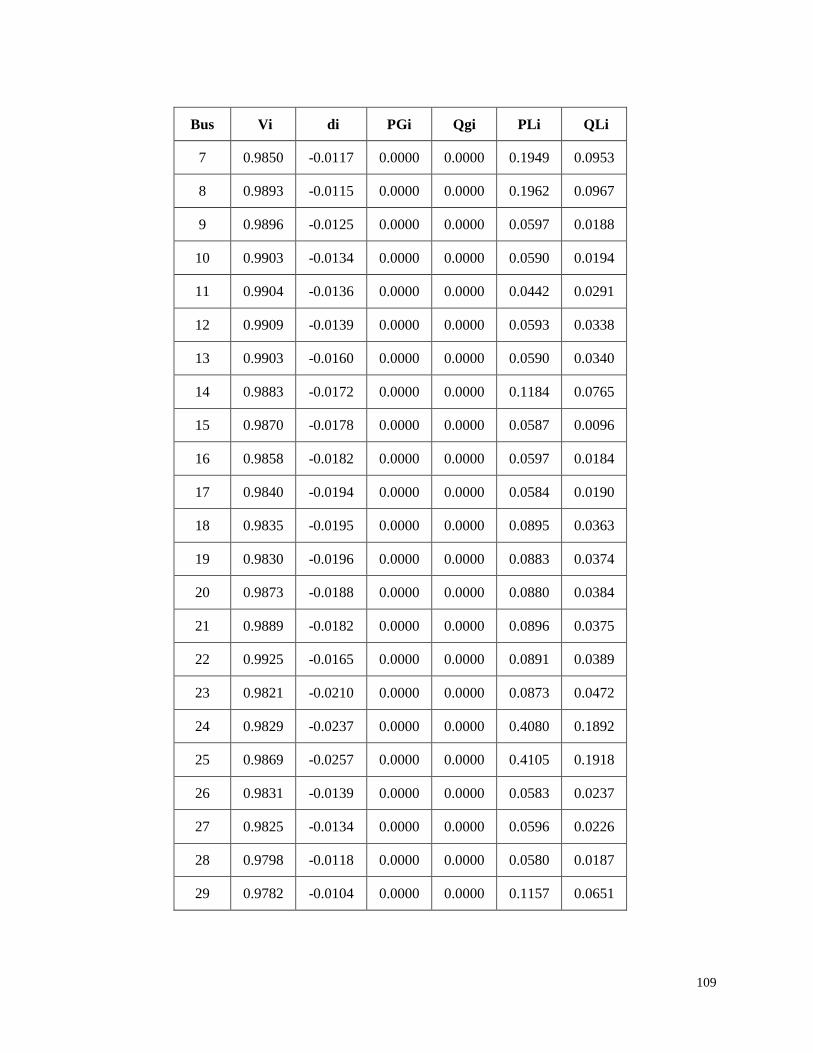
109
Bus Vi di PGi Qgi PLi QLi
7 0.9850 -0.0117 0.0000 0.0000 0.1949 0.0953
8 0.9893 -0.0115 0.0000 0.0000 0.1962 0.0967
9 0.9896 -0.0125 0.0000 0.0000 0.0597 0.0188
10 0.9903 -0.0134 0.0000 0.0000 0.0590 0.0194
11 0.9904 -0.0136 0.0000 0.0000 0.0442 0.0291
12 0.9909 -0.0139 0.0000 0.0000 0.0593 0.0338
13 0.9903 -0.0160 0.0000 0.0000 0.0590 0.0340
14 0.9883 -0.0172 0.0000 0.0000 0.1184 0.0765
15 0.9870 -0.0178 0.0000 0.0000 0.0587 0.0096
16 0.9858 -0.0182 0.0000 0.0000 0.0597 0.0184
17 0.9840 -0.0194 0.0000 0.0000 0.0584 0.0190
18 0.9835 -0.0195 0.0000 0.0000 0.0895 0.0363
19 0.9830 -0.0196 0.0000 0.0000 0.0883 0.0374
20 0.9873 -0.0188 0.0000 0.0000 0.0880 0.0384
21 0.9889 -0.0182 0.0000 0.0000 0.0896 0.0375
22 0.9925 -0.0165 0.0000 0.0000 0.0891 0.0389
23 0.9821 -0.0210 0.0000 0.0000 0.0873 0.0472
24 0.9829 -0.0237 0.0000 0.0000 0.4080 0.1892
25 0.9869 -0.0257 0.0000 0.0000 0.4105 0.1918
26 0.9831 -0.0139 0.0000 0.0000 0.0583 0.0237
27 0.9825 -0.0134 0.0000 0.0000 0.0596 0.0226
28 0.9798 -0.0118 0.0000 0.0000 0.0580 0.0187
29 0.9782 -0.0104 0.0000 0.0000 0.1157 0.0651

110
Bus Vi di PGi Qgi PLi QLi
30 0.9750 -0.0090 0.0000 0.0000 0.1919 0.5522
31 0.9713 -0.0103 0.0000 0.0000 0.1456 0.0624
32 0.9705 -0.0107 0.0000 0.0000 0.2037 0.0889
33 0.9703 -0.0108 0.0000 0.0000 0.0572 0.0362
34 0.9837 -0.0142 0.0000 0.0000 0.0596 0.0182
35 0.9827 -0.0197 0.0000 0.0000 0.0981 0.0561
36 0.9822 -0.0196 0.0000 0.0000 0.0894 0.0360
37 0.9823 -0.0185 0.0000 0.0000 0.1165 0.0755
38 0.9827 -0.0174 0.0000 0.0000 0.0589 0.0280
Total PG QG PL QL f Ploss
3.6850 2.2008 3.6304 2.1508 0.9971 0.0546
TABLE III. LOAD FLOW RESULT OF ITERATION 2 (OPTIMAL OPERATING POINT), PU
Bus Vi di PGi Qgi PLi QLi
1 1.0030 0.0000 0.7437 0.4201 0.0000 0.0000
2 0.9952 0.0068 0.8161 0.4453 0.0000 0.0000
3 0.9972 -0.0035 0.7279 0.3830 0.0000 0.0000
4 0.9974 -0.0004 0.6655 0.2515 0.0000 0.0000
5 0.9924 -0.0126 0.7288 0.7028 0.0000 0.0000
6 0.9838 -0.0075 0.0000 0.0000 0.0000 0.0000
7 0.9853 -0.0032 0.0000 0.0000 0.1950 0.0954
8 0.9886 -0.0041 0.0000 0.0000 0.1960 0.0964
9 0.9893 -0.0043 0.0000 0.0000 0.0597 0.0188
10 0.9905 -0.0045 0.0000 0.0000 0.0590 0.0194

111
Bus Vi di PGi Qgi PLi QLi
11 0.9908 -0.0045 0.0000 0.0000 0.0442 0.0292
12 0.9914 -0.0047 0.0000 0.0000 0.0594 0.0339
13 0.9917 -0.0049 0.0000 0.0000 0.0591 0.0341
14 0.9897 -0.0061 0.0000 0.0000 0.1185 0.0769
15 0.9884 -0.0067 0.0000 0.0000 0.0588 0.0096
16 0.9872 -0.0071 0.0000 0.0000 0.0597 0.0186
17 0.9853 -0.0082 0.0000 0.0000 0.0585 0.0191
18 0.9848 -0.0084 0.0000 0.0000 0.0895 0.0366
19 0.9842 -0.0073 0.0000 0.0000 0.0884 0.0376
20 0.9890 -0.0052 0.0000 0.0000 0.0883 0.0386
21 0.9908 -0.0041 0.0000 0.0000 0.0896 0.0379
22 0.9946 -0.0017 0.0000 0.0000 0.0893 0.0392
23 0.9831 -0.0089 0.0000 0.0000 0.0875 0.0473
24 0.9839 -0.0112 0.0000 0.0000 0.4087 0.1898
25 0.9879 -0.0127 0.0000 0.0000 0.4112 0.1925
26 0.9832 -0.0039 0.0000 0.0000 0.0583 0.0237
27 0.9828 -0.0031 0.0000 0.0000 0.0596 0.0226
28 0.9806 -0.0002 0.0000 0.0000 0.0581 0.0188
29 0.9794 0.0021 0.0000 0.0000 0.1159 0.0654
30 0.9762 0.0036 0.0000 0.0000 0.1923 0.5544
31 0.9725 0.0022 0.0000 0.0000 0.1458 0.0627
32 0.9717 0.0018 0.0000 0.0000 0.2039 0.0893
33 0.9714 0.0017 0.0000 0.0000 0.0573 0.0364

112
Bus Vi di PGi Qgi PLi QLi
34 0.9837 -0.0044 0.0000 0.0000 0.0596 0.0182
35 0.9838 -0.0075 0.0000 0.0000 0.0982 0.0563
36 0.9831 -0.0078 0.0000 0.0000 0.0895 0.0362
37 0.9829 -0.0070 0.0000 0.0000 0.1166 0.0757
38 0.9831 -0.0063 0.0000 0.0000 0.0589 0.0281
Total PG QG PL QL f Ploss
3.6820 2.2027 3.6343 2.1588 0.9971 0.0478
II.2. 6_bus test system
TABLE IV. GENERAL RESULT OF OPTIMAL LOAD FLOW ON 6_BUS SYSTEM
N0.
Iteration
Load flow, pu Optimization, pu
Number PGi KG Ploss (calculated
by B coefficients) PGinew KGnew
1
1(Droop) 0.3916 401.0638 0.0265391 0.3978 407.375
2(Droop) 0.3916 401.0638 0.3016 308.8672
3(Droop) 0.3916 401.0638 0.4747 486.2074
2
1(Droop) 0.3978 407.3750 0.0241074 0.3968 406.3396
2(Droop) 0.3016 308.8672 0.2165 221.7403
3(Droop) 0.4748 486.2074 0.5599 573.4366
3
1(Droop) 0.3972 406.3396 0.0228142
2(Droop) 0.2167 221.7403
3(Droop) 0.5605 573.4366
TABLE V. LOAD FLOW RESULT OF ITERATION 1 (INITIAL OPERATING POINT), PU

113
Bus Vi di PGi Qgi PLi Qli
1 0.9892 0.0000 0.3916 0.1904 0.0000 0.0000
2 0.9920 -0.0066 0.3916 0.1416 0.0000 0.0000
3 0.9730 -0.0497 0.3916 0.4781 0.0000 0.0000
4 0.9620 0.0011 0.0000 0.0000 0.4899 0.3242
5 0.9745 -0.0083 0.0000 0.0000 0.0000 0.0000
6 0.9674 -0.0464 0.0000 0.0000 0.6585 0.4654
Total PG QG PL QL f Ploss
1.1748 0.8101 1.1484 0.7896 0.9990 0.0264
TABLE VI. LOAD FLOW RESULT OF ITERATION 2, PU
Bus Vi di PGi Qgi PLi Qli
1 0.9901 0.0000 0.3978 0.1745 0.0000 0.0000
2 0.9901 -0.0122 0.3016 0.1750 0.0000 0.0000
3 0.9742 -0.0396 0.4748 0.4557 0.0000 0.0000
4 0.9630 0.0000 0.0000 0.0000 0.4908 0.3248
5 0.9754 -0.0109 0.0000 0.0000 0.0000 0.0000
6 0.9680 -0.0368 0.0000 0.0000 0.6592 0.4659
Total PG QG PL QL f Ploss
1.1741 0.8053 1.1501 0.7908 0.9990 0.0241
TABLE VII. LOAD FLOW RESULT OF ITERATION 3 (OPTIMAL OPERATING POINT), PU
Bus Vi di PGi Qgi PLi Qli
1 0.9906 0.0000 0.3972 0.1659 0.0000 0.0000

114
Bus Vi di PGi Qgi PLi Qli
2 0.9885 -0.0162 0.2167 0.2040 0.0000 0.0000
3 0.9755 -0.0278 0.5605 0.4327 0.0000 0.0000
4 0.9637 -0.0005 0.0000 0.0000 0.4916 0.3253
5 0.9765 -0.0122 0.0000 0.0000 0.0000 0.0000
6 0.9685 -0.0256 0.0000 0.0000 0.6600 0.4665
Total PG QG PL QL f Ploss
1.1744 0.8026 1.1516 0.7918 0.9990 0.0228

115
III. CHAPTER 4
III.1. Accuracy of results
III.1.1. Electrical data of 6_bus test system
TABLE I. BUS DATAS OF 6_BUS TEST SYSTEM, TAKING INTO ACCOUNT KGS
Bus
number
Load, pu Generator, pu Exponent of
Loads
P Q Kdi VG0i f0i/pu Alpha Beta
1 0.000000000 0.000000000 5.00 1.07 1.07 0.00 0.00
2 0.000000000 0.000000000 5.00 1.07 1.07 0.00 0.00
3 0.000000000 0.000000000 5.00 1.07 1.07 0.00 0.00
4 0.529334489 0.350297754 0.00 1.00 2.00 2.00
5 0.000000000 0.000000000 0.00 1.00 2.00 2.00
6 0.351794954 0.248636718 0.00 1.00 2.00 2.00
TABLE II. LINES DATAS OF 6_BUS TEST SYSTEM, TAKING INTO ACCOUNT KGS
Bus nl Bus nr R, pu X, pu
4 5 0.08128544 0.02266228
4 1 0.05671078 0.02494276
5 2 0.03780718 0.01781626
5 6 0.02835539 0.13134145
6 3 0.00945180 0.00356325
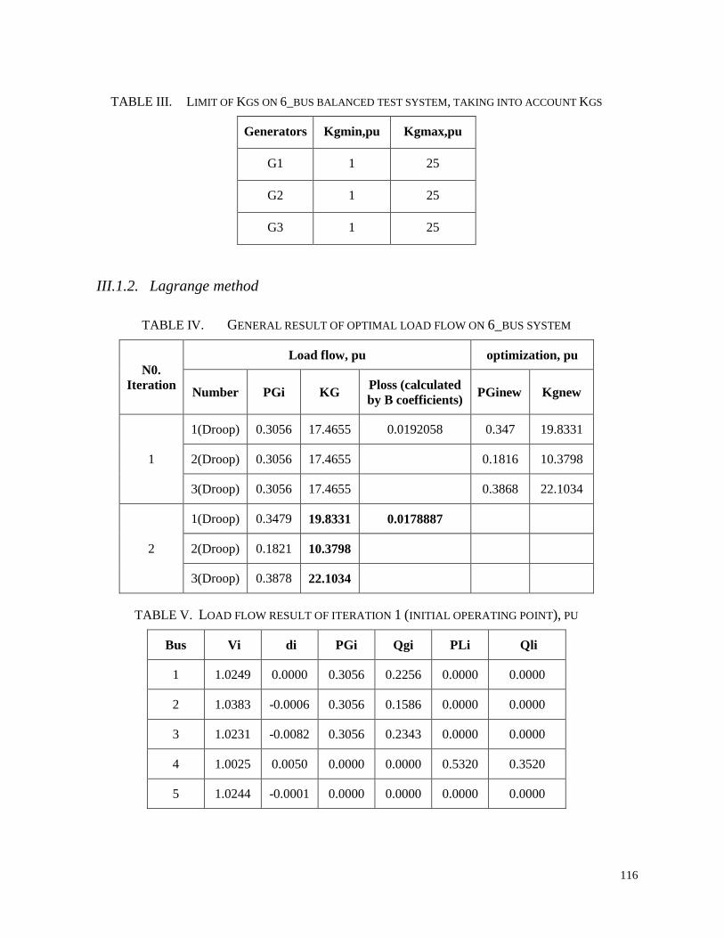
116
TABLE III. LIMIT OF KGS ON 6_BUS BALANCED TEST SYSTEM, TAKING INTO ACCOUNT KGS
Generators Kgmin,pu Kgmax,pu
G1 1 25
G2 1 25
G3 1 25
III.1.2. Lagrange method
TABLE IV. GENERAL RESULT OF OPTIMAL LOAD FLOW ON 6_BUS SYSTEM
N0.
Iteration
Load flow, pu optimization, pu
Number PGi KG Ploss (calculated
by B coefficients) PGinew Kgnew
1
1(Droop) 0.3056 17.4655 0.0192058 0.347 19.8331
2(Droop) 0.3056 17.4655 0.1816 10.3798
3(Droop) 0.3056 17.4655 0.3868 22.1034
2
1(Droop) 0.3479 19.8331 0.0178887
2(Droop) 0.1821 10.3798
3(Droop) 0.3878 22.1034
TABLE V. LOAD FLOW RESULT OF ITERATION 1 (INITIAL OPERATING POINT), PU
Bus Vi di PGi Qgi PLi Qli
1 1.0249 0.0000 0.3056 0.2256 0.0000 0.0000
2 1.0383 -0.0006 0.3056 0.1586 0.0000 0.0000
3 1.0231 -0.0082 0.3056 0.2343 0.0000 0.0000
4 1.0025 0.0050 0.0000 0.0000 0.5320 0.3520
5 1.0244 -0.0001 0.0000 0.0000 0.0000 0.0000
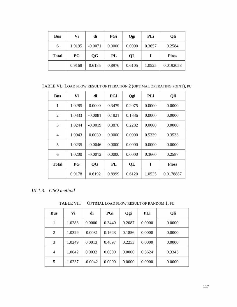
117
Bus Vi di PGi Qgi PLi Qli
6 1.0195 -0.0071 0.0000 0.0000 0.3657 0.2584
Total PG QG PL QL f Ploss
0.9168 0.6185 0.8976 0.6105 1.0525 0.0192058
TABLE VI. LOAD FLOW RESULT OF ITERATION 2 (OPTIMAL OPERATING POINT), PU
Bus Vi di PGi Qgi PLi Qli
1 1.0285 0.0000 0.3479 0.2075 0.0000 0.0000
2 1.0333 -0.0081 0.1821 0.1836 0.0000 0.0000
3 1.0244 -0.0019 0.3878 0.2282 0.0000 0.0000
4 1.0043 0.0030 0.0000 0.0000 0.5339 0.3533
5 1.0235 -0.0046 0.0000 0.0000 0.0000 0.0000
6 1.0200 -0.0012 0.0000 0.0000 0.3660 0.2587
Total PG QG PL QL f Ploss
0.9178 0.6192 0.8999 0.6120 1.0525 0.0178887
III.1.3. GSO method
TABLE VII. OPTIMAL LOAD FLOW RESULT OF RANDOM 1, PU
Bus Vi di PGi Qgi PLi Qli
1 1.0283 0.0000 0.3440 0.2087 0.0000 0.0000
2 1.0329 -0.0081 0.1643 0.1856 0.0000 0.0000
3 1.0249 0.0013 0.4097 0.2253 0.0000 0.0000
4 1.0042 0.0032 0.0000 0.0000 0.5624 0.3343
5 1.0237 -0.0042 0.0000 0.0000 0.0000 0.0000

118
Bus Vi di PGi Qgi PLi Qli
6 1.0204 0.0019 0.0000 0.0000 0.3859 0.2450
Total PG QG PL QL f Ploss
0.9180 0.6195 0.9001 0.6122 1.0536 0.0178565
TABLE VIII. OPTIMAL LOAD FLOW RESULT OF RANDOM 2, PU
Bus Vi di PGi Qgi PLi QLi
1 1.0283 0.0000 0.3439 0.2087 0.0000 0.0000
2 1.0329 -0.0081 0.1638 0.1856 0.0000 0.0000
3 1.0250 0.0014 0.4103 0.2252 0.0000 0.0000
4 1.0042 0.0032 0.0000 0.0000 0.5338 0.3533
5 1.0237 -0.0042 0.0000 0.0000 0.0000 0.0000
6 1.0204 0.0020 0.0000 0.0000 0.3663 0.2589
Total PG QG PL QL f Ploss
0.9180 0.6195 0.9001 0.6122 1.0531 0.0178565
TABLE IX. OPTIMAL LOAD FLOW RESULT OF RANDOM 3, PU
Bus Vi di PGi Qgi PLi Qli
1 1.0283 0.0000 0.3439 0.2087 0.0000 0.0000
2 1.0329 -0.0081 0.1641 0.1856 0.0000 0.0000
3 1.0250 0.0013 0.4099 0.2252 0.0000 0.0000
4 1.0042 0.0032 0.0000 0.0000 0.5338 0.3533
5 1.0237 -0.0042 0.0000 0.0000 0.0000 0.0000
6 1.0204 0.0020 0.0000 0.0000 0.3663 0.2589

119
Bus Vi di PGi Qgi PLi Qli
Total PG QG PL QL f Ploss
0.9180 0.6195 0.9001 0.6122 1.0527 0.0178565
TABLE X. OPTIMAL LOAD FLOW RESULT OF RANDOM 4, PU
Bus Vi di PGi Qgi PLi Qli
1 1.0283 0.0000 0.3439 0.2087 0.0000 0.0000
2 1.0329 -0.0081 0.1639 0.1856 0.0000 0.0000
3 1.0250 0.0014 0.4102 0.2252 0.0000 0.0000
4 1.0042 0.0032 0.0000 0.0000 0.5338 0.3533
5 1.0237 -0.0042 0.0000 0.0000 0.0000 0.0000
6 1.0204 0.0020 0.0000 0.0000 0.3663 0.2589
Total PG QG PL QL f Ploss
0.9180 0.6195 0.9001 0.6122 1.0520 0.0178565
TABLE XI. OPTIMAL LOAD FLOW RESULT OF RANDOM 5, PU
Bus Vi di PGi Qgi PLi QLi
1 1.0283 0.0000 0.3439 0.2087 0.0000 0.0000
2 1.0329 -0.0081 0.1639 0.1856 0.0000 0.0000
3 1.0250 0.0014 0.4102 0.2252 0.0000 0.0000
4 1.0042 0.0032 0.0000 0.0000 0.5338 0.3533
5 1.0237 -0.0042 0.0000 0.0000 0.0000 0.0000
6 1.0204 0.0020 0.0000 0.0000 0.3663 0.2589
Total PG QG PL QL f Ploss
0.9180 0.6195 0.9001 0.6122 1.0535 0.0178565

120
III.2. Other applications with variable KGs and Kds
TABLE XII. BUS DATAS OF 6_ BUS TEST SYSTEM, TAKING INTO ACCOUNT KGS AND KDS
Bus
number
Type
generator
Load, pu Generator, pu Exponent of Loads
P Q VG0i f0i/pu Alpha Beta
1 Droop 0.000000000 0.000000000 0.9877 1 0 0
2 Droop 0.000000000 0.000000000 0.9877 1 0 0
3 Droop 0.000000000 0.000000000 0.9877 1 0 0
4 0.052900000 0.000000000 0 1 2 2
5 0.052900000 0.000000000 0 1 2 2
6 0.027872043 0.026411745 0 1 2 2
7 0.000000000 0.000000000 0 1 2 2
8 0.000000000 0.000000000 0 1 2 2
9 0.000000000 0.000000000 0 1 2 2
TABLE XIII. LINES DATAS OF 6_BUS TEST SYSTEM, TAKING INTO ACCOUNT KGS AND KDS, PU
Bus nl Bus nr R, pu X, pu
4 5 0.02835539 0.00441843
4 1 0.02835539 0.00441843
5 2 0.02835539 0.00441843
5 6 0.02835539 0.00441843
6 3 0.02835539 0.00441843
1 7 0.01890359 0.28506011
2 8 0.01890359 0.28506011
3 9 0.01890359 0.28506011

121
TABLE XIV. LIMIT OF KGS ON 6_BUS TEST SYSTEM TAKING INTO ACCOUNT KGS AND KDS, PU
Generators KGmin KGmax Kdmin Kdmax
G1 6 16 6 16
G2 3 10 3 10
G3 6 16 6 16
TABLE XV. OPTIMAL LOAD FLOW RESULT OF RANDOM 1, PU
Bus Vi di PGi Qgi PLi Qli
1 0.9869 0.0000 0.0491 0.0049 0.0000 0.0000
2 0.9868 0.0001 0.0456 0.0060 0.0000 0.0000
3 0.9868 0.0002 0.0353 0.0148 0.0000 0.0000
4 0.9854 -0.0001 0.0000 0.0000 0.0514 0.0000
5 0.9855 0.0001 0.0000 0.0000 0.0514 0.0000
6 0.9857 0.0004 0.0000 0.0000 0.0271 0.0257
7 0.9869 0.0000 0.0000 0.0000 0.0000 0.0000
8 0.9868 0.0001 0.0000 0.0000 0.0000 0.0000
9 0.9868 0.0002 0.0000 0.0000 0.0000 0.0000
Total PG QG PL QL f Ploss
0.1300 0.0257 0.1298 0.0257 0.9949 0.00018143
TABLE XVI. OPTIMAL LOAD FLOW RESULT OF RANDOM 2, PU
Bus Vi di PGi Qgi PLi Qli
1 0.9869 0.0000 0.0493 0.0050 0.0000 0.0000
2 0.9868 0.0001 0.0453 0.0056 0.0000 0.0000
3 0.9868 0.0001 0.0355 0.0151 0.0000 0.0000

122
Bus Vi di PGi Qgi PLi Qli
4 0.9854 -0.0001 0.0000 0.0000 0.0514 0.0000
5 0.9855 0.0001 0.0000 0.0000 0.0514 0.0000
6 0.9857 0.0004 0.0000 0.0000 0.0271 0.0257
7 0.9869 0.0000 0.0000 0.0000 0.0000 0.0000
8 0.9868 0.0001 0.0000 0.0000 0.0000 0.0000
9 0.9868 0.0001 0.0000 0.0000 0.0000 0.0000
Total PG QG PL QL f Ploss
0.1300 0.0257 0.1298 0.0257 0.9952 0.00018140
TABLE XVII. OPTIMAL LOAD FLOW RESULT OF RANDOM 3, PU
Bus Vi di PGi Qgi PLi QLi
1 0.9869 0.0000 0.0492 0.0050 0.0000 0.0000
2 0.9868 0.0001 0.0452 0.0057 0.0000 0.0000
3 0.9868 0.0002 0.0356 0.0150 0.0000 0.0000
4 0.9854 -0.0001 0.0000 0.0000 0.0514 0.0000
5 0.9855 0.0001 0.0000 0.0000 0.0514 0.0000
6 0.9857 0.0004 0.0000 0.0000 0.0271 0.0257
7 0.9869 0.0000 0.0000 0.0000 0.0000 0.0000
8 0.9868 0.0001 0.0000 0.0000 0.0000 0.0000
9 0.9868 0.0002 0.0000 0.0000 0.0000 0.0000
Total PG QG PL QL f Ploss
0.1300 0.0257 0.1298 0.0257 0.9953 0.00018140

123
TABLE XVIII. OPTIMAL LOAD FLOW RESULT OF RANDOM 4, PU
Bus Vi di PGi Qgi PLi QLi
1 0.9869 0.0000 0.0492 0.0046 0.0000 0.0000
2 0.9869 0.0001 0.0457 0.0066 0.0000 0.0000
3 0.9868 0.0002 0.0351 0.0145 0.0000 0.0000
4 0.9855 -0.0001 0.0000 0.0000 0.0514 0.0000
5 0.9855 0.0001 0.0000 0.0000 0.0514 0.0000
6 0.9857 0.0004 0.0000 0.0000 0.0271 0.0257
7 0.9869 0.0000 0.0000 0.0000 0.0000 0.0000
8 0.9869 0.0001 0.0000 0.0000 0.0000 0.0000
9 0.9868 0.0002 0.0000 0.0000 0.0000 0.0000
Total PG QG PL QL f Ploss
0.1300 0.0257 0.1298 0.0257 0.9952 0.00018147
TABLE XIX. OPTIMAL LOAD FLOW RESULT OF RANDOM 5, PU
Bus Vi di PGi Qgi PLi QLi
1 0.9869 0.0000 0.0492 0.0050 0.0000 0.0000
2 0.9868 0.0001 0.0451 0.0058 0.0000 0.0000
3 0.9868 0.0002 0.0358 0.0148 0.0000 0.0000
4 0.9854 -0.0001 0.0000 0.0000 0.0514 0.0000
5 0.9855 0.0001 0.0000 0.0000 0.0514 0.0000
6 0.9857 0.0004 0.0000 0.0000 0.0271 0.0257
7 0.9869 0.0000 0.0000 0.0000 0.0000 0.0000
8 0.9868 0.0001 0.0000 0.0000 0.0000 0.0000
9 0.9868 0.0002 0.0000 0.0000 0.0000 0.0000

124
Total PG QG PL QL f Ploss
0.1300 0.0257 0.1298 0.0257 0.9953 0.00018141

125
III.3. Applications considering frequency and line ampacity constraints
III.3.1. Application with variables KGs
TABLE XX. BUS DATAS OF 6_BUS TEST SYSTEM, TAKING INTO ACCOUNT CONSTRAINED FREQUENCY
AND LINE AMPACITY WITH VARIABLES ARE KGS, PU
Bus
number
Type
generator
Load, pu Generator, pu Exponent of Loads
P Q Kdi VG0i f0i/pu Alpha Beta
1 Droop 0.0000 0.0000 5 1.07 1.03 0 0
2 Droop 0.0000 0.0000 5 1.07 1.03 0 0
3 Droop 0.0000 0.0000 5 1.07 1.03 0 0
4 0.5293 0.3532 0.00 1.00 2.00 2.00
5 0.2486 0.1486 0.00 1.00 2.00 2.00
6 0.3518 0.2486 0.00 1.00 2.00 2.00
TABLE XXI. LINES DATAS OF 6_BUS TEST SYSTEM, TAKING INTO ACCOUNT CONSTRAINED
FREQUENCY AND LINE AMPACITY WITH VARIABLES ARE KGS
Bus nl Bus nr R, pu X, pu
4 5 0.08128544 0.02266228
4 1 0.05671078 0.02494276
5 2 0.05671078 0.02494276
5 6 0.08128544 0.02266228
6 3 0.05671078 0.02494276
TABLE XXII. OPTIMAL CURRENT LINE RESULT OF CASE 1, PU
Bus
nl Bus nr I opt case 1 DelI Imax case 1
4 5 0.1254 0.2746 0.4000

126
Bus
nl Bus nr I opt case 1 DelI Imax case 1
4 1 0.4998 0.0002 0.5000
5 2 0.4103 0.0897 0.5000
5 6 0.0116 0.3884 0.4000
6 3 0.4247 0.0753 0.5000
TABLE XXIII. OPTIMAL LOAD FLOW RESULT OF CASE 1, PU
Bus Vi di PGi Qgi PLi QLi
1 1.0107 0.0000 0.3711 0.2965 0.0000 0.0000
2 1.0219 0.0018 0.3670 0.2403 0.0000 0.0000
3 1.0244 0.0060 0.3849 0.2280 0.0000 0.0000
4 0.9826 0.0076 0.0000 0.0000 0.5015 0.3473
5 0.9957 0.0062 0.0000 0.0000 0.2419 0.1501
6 0.9975 0.0093 0.0000 0.0000 0.3436 0.2520
Total PG QG PL QL f Ploss
1.1229 0.7648 1.0870 0.7494 0.9814 0.0359207
TABLE XXIV. OPTIMAL CURRENT LINE RESULT OF CASE 2, PU
Bus nl Bus nr I opt case 2 DelI Imax case 2
4 5 0.1564 0.1436 0.3000
4 1 0.4700 0.0000 0.4700
5 2 0.4292 0.0708 0.5000
5 6 0.0420 0.2580 0.3000
6 3 0.4367 0.1633 0.6000

127
TABLE XXV. OPTIMAL LOAD FLOW RESULT OF CASE 2, PU
Bus Vi di PGi Qgi PLi QLi
1 1.0163 0.0000 0.4311 0.2686 0.0000 0.0000
2 1.0196 -0.0066 0.3340 0.2520 0.0000 0.0000
3 1.0209 -0.0047 0.3575 0.2453 0.0000 0.0000
4 0.9856 0.0045 0.0000 0.0000 0.5043 0.3497
5 0.9949 -0.0008 0.0000 0.0000 0.2413 0.1499
6 0.9951 0.0002 0.0000 0.0000 0.3417 0.2509
Total PG QG PL QL f Ploss
1.1225 0.7658 1.0873 0.7506 0.9808 0.0352283
III.3.2. Applications with variables KGs and Kds
TABLE XXVI. OPTIMAL CURRENT LINE RESULT OF CASE 1, PU
Bus nl Bus nr I opt case 1 DelI Imax case 1
4 5 0.1280 0.2720 0.4000
4 1 0.4946 0.0054 0.5000
5 2 0.4143 0.0857 0.5000
5 6 0.0020 0.3980 0.4000
6 3 0.4247 0.0753 0.5000
TABLE XXVII. OPTIMAL LOAD FLOW RESULT OF CASE 1, PU
Bus Vi di PGi Qgi PLi QLi
1 1.0082 0.0000 0.4205 0.2680 0.0000 0.0000
2 1.0133 -0.0034 0.3529 0.2275 0.0000 0.0000
3 1.0137 -0.0042 0.3540 0.2452 0.0000 0.0000

128
Bus Vi di PGi Qgi PLi QLi
4 0.9779 0.0048 0.0000 0.0000 0.5024 0.3403
5 0.9879 0.0007 0.0000 0.0000 0.2408 0.1461
6 0.9879 0.0009 0.0000 0.0000 0.3408 0.2444
Total PG QG PL QL f Ploss
1.1273 0.7407 1.0841 0.7308 0.9926 0.0351713