Embed Size (px)
Citation preview
Int. J. Production Economics 130 (2011) 27–32
Contents lists available at ScienceDirect
Int. J. Production Economics
0925-52
doi:10.1
n Tel.:
E-m
journal homepage: www.elsevier.com/locate/ijpe
Optimal policy for a mixed production system with multiple OEM andOBM products
Bin Zhang n
Lingnan College, Sun Yat-Sen University, Guangzhou 510275, P.R. China
a r t i c l e i n f o
Article history:
Received 10 July 2009
Accepted 12 October 2010Available online 20 October 2010
Keywords:
Mixed production
OEM
OBM
Capacity constraint
Newsboy
73/$ - see front matter & 2010 Elsevier B.V. A
016/j.ijpe.2010.10.010
+86 20 84110649; fax: +86 20 84114823.
ail address: [email protected]
a b s t r a c t
In the process of manufacture upgrade from original equipment manufacture (OEM) to own brand
manufacture (OBM), the parallel OEM and OBM strategy is an important strategic choice for many
manufacturing companies. This paper considers a mixed production system under this parallel strategy.
The mixed system uses the common production capacity to produce multiple OEM and OBM products for
fulfilling independent demands. A profit-maximization model is proposed for the mixed production
problem. The structural properties of the solution and an efficient solution method for solving the
proposed model are developed. Numerical results are provided for showing the efficiency of the proposed
solution method and obtaining some managerial insights.
& 2010 Elsevier B.V. All rights reserved.
1. Introduction
The original equipment manufacture (OEM) suppliers play animportant role in global economy. In recent decades, most of thewell-known manufacturing companies in developing countries,especially in East Asia, specialized as global manufacturing serviceproviders under OEM contract arrangements (Lian, 2007). Manu-facturing companies from South Korea, Taiwan, Chinese Mainland,Vietnam, etc., were authorized by firms from developed countrieswhich suffered from high production costs at their own countries toproduce their required products. The use of OEM contracts helpedmanufacturing companies in developing countries enter globalmarkets with minimum efforts. Many manufacturing firms usedOEM to address entry barriers during their early period of inter-nationalization, such as LG Electronics, Giant Manufacturing, etc.(Cheng et al., 2005).
OEM is an important strategy for latecomers in their inter-nationalization due to its various advantages, such as avoiding highR&D cost and cost of sales, reducing risk of product developmentfailure, achieving economies of scale, utilizing idle produc-tion capacity, and generating short-term revenue (Chen, 1989;Li, 2006). The implementation of OEM strategy needs some compara-tive advantages, such as cheaper labor cost, appreciating currency,and excellent quality of products. Unfortunately, some of theseadvantages are not durative, and original equipment manufacturersoften need reconfiguration of their supply chain (Komoto et al., 2009).In recent years, many OEM suppliers in Taiwan and Chinese Mainlandsuffered in the situation of comparative advantage decline, with a
ll rights reserved.
stabilizing economic growth, rising labor cost, an appreciatingcurrency, tighter environmental protection measures, and moreintense competition. All these factors made the OEM strategy lessprofitable (Jin, 2008). Recently, the current world financial crisis cutsdown OEM orders; many OEM firms have been shut down, especiallyin Chinese toy and clothing industries.
In order to gain competitive advantage during the process ofglobalization, OEM suppliers have attempted manufacture upgradedeveloping their own brands for achieving higher added values(Chu, 2009). The process of manufacture upgrade can be describedas progression along the value creation chain from own equipmentmanufacturing to own brand manufacturing (OBM) (Humphrey,2004). Manufacture upgrade helped a lot of firms includingSamsung Electronics, Hyundai Motors and LG Electronics, ASUS,Acer, BenQ and Giant Manufacturing achieve high success in theirglobal business operations (Chu, 2009). A focus on China’s experi-ence in manufacture upgrade is timely and noteworthy. Because italways takes quite some time for firms to upgrade from OEM toOBM, and it is a high-risk practice to completely give up OEMproduction and switch to OBM strategy, many OEM suppliers chosethe parallel OEM and OBM strategy.
The parallel OEM and OBM strategy has more flexibility thanpure OEM or OBM strategy. Under this parallel strategy, the firmscan concentrate on OBM if the own brands begin to obtain stableand high profit; they can utilize the idle production capacity onOEM products for generating short-term revenue if the marketshare of own brand products is not ideal in a short period. In themeanwhile, the marketing expense for OBM can be supported bythe stable revenue from OEM orders, and the firms can also learnnew technologies and experience through OEM production(Li, 1992). The parallel OEM and OBM strategy was successfullyimplemented by many firms in East Asia, such as ASUS and Acer
B. Zhang / Int. J. Production Economics 130 (2011) 27–3228
in Taiwan, Glanz in China, etc. Although the parallel OEM and OBMstrategy is getting more popular in East Asia, and the relationshipbetween OEM and OBM has been substantially discussed in recentyears (Lian, 2007), most studies in literature examined manufac-ture upgrade in terms of economic conditions, institutional char-acteristics, and entrepreneurial growth strategy and marketingcapabilities (e.g., McDougall et al., 1994; Cheng et al., 2005;Li, 2006; Tan, 2007; Eng and Spickett-Jones, 2009), little workhas been done for investigating the mixed production decisionsunder the parallel OEM and OBM strategy.
This paper considers a mixed production system under theparallel OEM and OBM strategy. The mixed system uses thecommon production capacity to fulfill demands for multipleOEM and OBM products. Demands for OEM products are determi-nistic before production since OEM orders are often arranged insubcontracts. Demands for OBM products are often uncertainbefore the sale season. The mixed production system makes theoptimal production decisions more challenging in multi-productsettings. On the one hand, the use of OEM production for achievinga certain profit should be properly balanced against possible lossfrom unsatisfied demand on OBM markets; on the other hand, thelimited capacity should be well allocated to different OEM and OBMproducts. The overall objective is to decide the optimal productionquantities of OEM and OBM products for maximizing the totalexpected profit. We establish the structural properties for theoptimal decisions and develop an exact solution method for thestudied problem.
This rest of the paper is organized as follows. Section 2 describesthe mixed production problem. In Section 3, the structural proper-ties are investigated. Section 4 proposes the solution method.Numerical experiment is described in Section 5 for showing theeffectiveness of the proposed solution method and obtaining somemanagerial insights. Section 6 concludes the paper with a fewfuture research directions. All proofs are presented in the Appendix.
2. Problem formulation
Consider a mixed production system that uses the commoncapacity to produce n different OBM products, and m different OEMproducts. Let i¼1,y,n be the index for all OBM products, andi¼n+1,y,n+m for OEM products. We use the following costparameters:
ci¼unit production cost for product i¼1,y,n+m;pi¼unit selling price for product i¼1,y,n+m;si¼unit salvage value for OBM product i¼1,y,n.
To avoid the trivial case, we assume pi4ci4si, i¼1,y,n andpi4ci, i¼n+1,y,n+m. That is to say, the selling price is larger thanthe production cost for any OEM and OBM product, and theproduction cost for any OBM product is larger than the correspond-ing salvage value.
Let Di denote the random demand for OBM product i¼1,y,n,which has a continuous probability density function fi(U), cumu-lative distribution function Fi(U), and reverse distribution functionF�1
i ðUÞ, and let di be the deterministic demand for OEM producti¼n+1,y,n+m. It is not uncommon to assume that all demands arenon-negative, so we assume that Fi(x)¼0 for all xo0, and Fi(0)Z0,i¼1,y,n, and diZ0, i¼n+1,y,n+m. Although Fi(0)¼0 technicallyrules out normal distribution as well as many other distributionswith negative support values, some approximating or truncatedtechniques can provide good demand approximations for thesedistributions (Zhang and Du, 2010).
We further assume that demands for all OBM and OEM productscan be partly fulfilled. The demands for OBM products exceeding
the production quantities will be lost or backordered, and themanufacturer can accept and satisfy part of the OEM demands.The manufacturer’s decisions are made as follows. At time zero, themanufacturer receives demand forecasts for all OBM products andthe subcontract requirements for all OEM products. The manufac-turer makes OBM production decisions (x1,y,xn) and determinesthe quantities (xn+ 1,y,xn +m) accepted for OEM productionsubcontracts. At time t, the manufacturer receives the actualdelivering orders and delivers the products. The overallobjective of the manufacturer is to decide the optimal productionquantities x¼(x1,y,xn,xn + 1,y,xn +m) so as to maximize the totalexpected profit.
The production of OBM and OEM products consumes someproduction capacities which may include product-specific capa-cities and one common capacity. To express the product-specificcapacity constraint, we introduce an upper bound ui40 for theproduction decision xi, i¼1,y,n+m, i.e., xirui. To reflect thecommon capacity constraint, we assume that each OBM or OEMproduct requires a deterministic production time ti40 when usingthe common capacity. Since the length of the available productionperiod is t, the common capacity constraint can be written asPnþm
i ¼ 1 tixirt.Since the manufacturer will never produce OEM products that
cannot be sold (with certainty), the OEM production quantityshould satisfy xirdi, i¼n+1,y,n+m. To simplify the expression ofthese constraints, we define a new upper bound as follows:
zi ¼ui,i¼ 1,. . .,n,
minðui,diÞ,i¼ nþ1,. . .,nþm:
(ð1Þ
Eq. (1) implies that each OBM production quantity should beupper bounded by the product-specific capacity and that each OEMproduction quantity should not be larger than the minimal value ofthe product-specific capacity and the subcontracting demand. ForOEM product i¼n+1,y,n+m, zi can be viewed as the active demandsince any demand exceeding zi must be lost or backordered becauseof the limited product-specific capacity.
Now we are ready to present the optimization model for themixed production problem. Let (U)+
¼max{U,0}; the mathematicalmodel for maximizing the total expected profit is given as follows(denoted as problem P):
maxp¼Xn
i ¼ 1
EDipi minðxi,DiÞþsiðxi�DiÞ
þ�cixi
� �þ
Xnþm
i ¼ nþ1
ðpi�ciÞxi,
ð2Þ
subject to
Xnþm
i ¼ 1
tixirt, ð3Þ
0rxirzi, i¼ 1,. . .,nþm: ð4Þ
In this model, pi min(xi,Di) is the revenue from OBM producti¼1,y,n; si(xi�Di)
+ is the salvage value of the excess OBM producti¼1,y,n; cixi is the production cost of OBM product i¼1,y,n; and(pi�ci)xi is the profit from OEM product i¼n+1,y,n+m. We denoteby gi¼(pi�ci)/ti the marginal common capacity benefit of producti¼1,y,n+m and re-index OEM products such that gn + 1Z?Zgn +m.
Problem P can also be viewed as a single-period constrainedinventory problem, in which deterministic and uncertain demandsrequire a common capacity. If all demands are deterministic, thenproblem P becomes a linear programming problem, which can beeasily solved using some solution packages, such as CPLEX.
If all demands are uncertain, then problem P becomes a multi-product newsboy problem with box constraints, which has been
B. Zhang / Int. J. Production Economics 130 (2011) 27–32 29
extensively studied in the last decades, for examples, see Hadleyand Whitin (1963), Erlebacher (2000), Vairaktarakis (2000), Moonand Silver (2000) and Abdel-Malek et al. (2004). Some of theexisting research ignored non-negativity constraints on productiondecisions. Hadley and Whitin (1963), Kabak and Weinberg (1972),Abdel-Malek and Montanari (2005), Niederhoff (2007) and Zhangand Du (2010) considered non-negativity constraints in someways. Recently, Zhang et al. (2009) developed an exact solutionmethod for the singly constrained multi-product newsboy problemwith non-negativity constraints. Most of these researches did notconsider the upper bounds on the decision variables. Zhang andHua (2008) proposed a unified algorithm for solving a class ofnonlinear knapsack problems, which can be directly applied tosolve the singly constrained multi-product newsboy problem withbox constraints. Zhang and Hua (2010) investigated an extendedmulti-product newsboy problem in which products are procuredthrough mixed wholesale price contracts and option contracts. Intheir model, some products are procured through option contracts,while in our model the certain demands for OEM products can bearranged through wholesale price contracts or option contracts.
Nonlinear optimization methods developed for solving multi-constraint problems could be possibly modified to solve problem P.However, specialized algorithms based on the structural propertiesare much faster and more reliable (Zhang and Hua, 2008; Zhang,2010). In literature, we have not found any efficient algorithm forsolving problem P.
3. Structural properties
In this section, we establish the structural properties of problemP. We start from the objective function of problem P. Usingmathematical manipulation, the expected profit of problem Pcan be rewritten as
p¼Xn
i ¼ 1
ðpi�ciÞxi�ðpi�siÞ
Z xi
0FiðziÞdzi
� �þ
Xnþm
i ¼ nþ1
ðpi�ciÞxi: ð5Þ
Then we have the following proposition:
Proposition 1. The expected profit function p is concave in xi,i¼1,y,n+m.
Since p is concave and the feasible domain is convex, theKarush–Kuhn–Tucker (KKT) conditions are necessary and suffi-cient for optimality. Let l be the dual variable corresponding to theconstraint in Eq. (3), and let wi and vi, i¼1,y,n+m be the dualvariables corresponding to the constraints 0rxi and xirzi,i¼1,y,n+m in Eq. (4) respectively. Thus, xi i¼1,y,n+m is theoptimal solution if and only if there exist non-negative dualvariables l, wi, and vi, i¼1,y,n+m, such that
ðpi�ciÞ�ðpi�siÞFiðxiÞ�ltiþwi�vi ¼ 0, i¼ 1,. . .,n, ð6Þ
ðpi�ciÞ�ltiþwi�vi ¼ 0, i¼ nþ1,. . .,nþm, ð7Þ
Xnþm
i ¼ 1
wixiþXnþm
i ¼ 1
viðzi�xiÞ ¼ 0, ð8Þ
l t�Xnþm
i ¼ 1
tixi
!¼ 0: ð9Þ
lZ0 in Eq. (9) represents the shadow price of the commoncapacity. l40 implies that the capacity constraint in Eq. (3) holdsas equality.
Let ~xi ¼minfF�1i ððpi�ciÞ=ðpi�siÞÞ,zig, i¼1,y,n, and ~xi ¼ zi, i¼n+1,
y,n+m. It can be easily verified that ~xi is the optimal solution toproblem P without the common capacity constraint in Eq. (3).
Denote by (xn,ln,wn,vn) a solution of KKT conditions in Eqs. (6)–(9),then we have the following proposition:
Proposition 2.
(a)
x�i r ~xi , i¼1,y,n+m;P (b) If nþmi ¼ 1 ti ~xirt, then x�i ¼ ~xi , i¼1,y,n+m;P P
(c) If nþmi ¼ 1 ti ~xi4t , then nþmi ¼ 1 tix
�i ¼ t .
Proposition 2(a) gives the maximal production quantities for allOBM and OEM products; Proposition 2(b) indicates that theoptimal solution to problem P is the same as that of the problemwithout the common capacity constraint, if the common capacityconstraint is not binding. Proposition 2(c) illustrates that thelimited common capacity must be fully utilized if there is noenough common capacity.
For any given lZ0, the following proposition defines a solutionto Eqs. (6)–(8)) as a function of the shadow price l, i.e., xi(l),i¼1,y,n+m.
Proposition 3. With any given lZ0, xi(l), i¼1,y,n+m, satisfies
Eqs. (6)–(8) if and only if
xiðlÞ ¼
0, if giol,
F�1i
pi�ci�lti
pi�si
� �, if gi�
ðpi�siÞFiðziÞ
tirlrgi,
zi, if gi�ðpi�siÞFiðziÞ
ti4l,
i¼ 1,. . .,n,
8>>>>><>>>>>:
ð10Þand
xiðlÞ ¼
0, if giol,
yi, if gi ¼ l,
zi, if gi4l,
i¼ nþ1,. . .,nþm,
8><>: ð11Þ
where yi is any real value over [0,zi], i¼n+1,y,n+m.
The results of Proposition 3 can be explained with somemanagerial insights. Consider the optimal decisions for OBMproducts; according to Zhang et al. (2009), we know that theoptimal solution to the unconstrained newsboy problem isxi ¼ F�1
i ððpi�ciÞ=ðpi�siÞÞ. Since ci+lti can be viewed as the adjustedproduction cost with the shadow price of the common capacity, theoptimal solution to newsboy problem with the common capacityconstraint is xiðlÞ ¼ F�1
i ððpi�ci�ltiÞ=ðpi�siÞÞ. If we further considerthe box constraint 0rxirzi, we have xiðlÞ ¼maxfminfF�1
i ððpi�
ci�ltiÞ=ðpi�siÞÞ,zig,0g. It is easily found that Eq. (10) is a detailedexpression of this equation.
Consider the optimal decisions for OEM product i¼n+1,y,n+m; Eq. (11) can be explained comparing the marginal commoncapacity benefit and the shadow price l. If the marginal commoncapacity benefit is smaller than the shadow price, i.e., giol, thenthe common capacity will never be used for producing OEMproduct i (xi(l)¼0); if the marginal common capacity benefit islarger than the shadow price, i.e., gi4l, then the common capacitywill be used to produce as much as possible OEM product i
(xi(l)¼zi); if the marginal common capacity benefit equals theshadow price, i.e., gi¼l, then the common capacity will be used toproduce any quantity yiA[0,zi].
According to Eq. (11), we know that the value of xi(l) cannot beuniquely determined if gi¼l* for some iA{n+1,y,n+m}. Let
k1 ¼ argmin i gi ¼ l�,i¼ nþ1,. . .,nþm��
,
ð12Þ
k2 ¼ argmax i gi ¼ l�,i¼ nþ1,. . .,nþm��
,
ð13Þ
Then we have k1rk2. k1¼k2 holds for the case that there is onlyone iA{n+1,y,n+m} such that gi¼l*. Since gn + 1Z?Zgn + m,
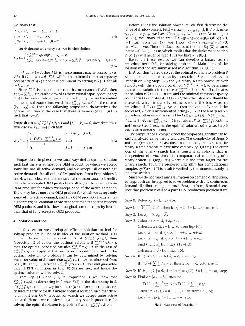
Fig. 1. Main steps of Algorithm 1.
B. Zhang / Int. J. Production Economics 130 (2011) 27–3230
we know that
gi4l�, i¼ nþ1,. . .,k1�1,
gi ¼ l�, i¼ k1,. . .,k2,
giol�, i¼ k2þ1,. . .,nþm
:
8><>: ð14Þ
Let F denote an empty set, we further define
GðlÞ ¼
Pnþmi ¼ 1 tixiðlÞ,iffk1,. . .,k2g ¼F,Pni ¼ 1 tixiðlÞþ
Pk1�1i ¼ nþ1 tixiðlÞþ
Pnþmi ¼ k2þ1 tixiðlÞ,iffk1,. . .,k2gaF:
(
ð15Þ
If {k1,y,k2}¼F, then G(l) is the common capacity occupancy ofx(l); if {k1,y,k2}aF, G(l) will be the minimal common capacityoccupancy of x(l) since it is equivalent to setting xi(l)¼0 for alli¼k1,y,k2.
Since G(l) is the minimal capacity occupancy of x(l), thenGðlÞþ
Pk2
i ¼ k1tizi can be viewed as the maximal capacity occupancy
of x(l), because it sets xi(l)¼zi for all i¼k1,y,k2. To use the unifiedmathematical expression, we define
Pk2
i ¼ k1tizi ¼ 0 for the case of
{k1,y,k2}¼F. Then the following proposition characterizes theoptimal solution in the case that there is some iA{n+1,y,n+m}such that gi¼l*.
Proposition 4. IfPnþm
i ¼ 1 ti ~xi4t and {k1,y,k2}aF, then there must
exist one kA{k1,y,k2} such that
x�i ðl�Þ ¼
zi, i¼ nþ1,. . .,k�1,
t�Gðl�Þ�Pk�1
i ¼ k1tizi
tk, i¼ k,
0, i¼ kþ1,. . .,nþm:
8>>><>>>:
ð16Þ
Proposition 4 implies that we can always find an optimal solution
such that there is at most one OEM product for which we accept
some but not all active demand, and we accept ‘‘all or nothing’’
active demands for all other OEM products. From Propositions 3
and 4, we can observe that the marginal common capacity benefits
of the fully accepted OEM products are all higher than that of those
OEM products for which we accept none of the active demands.
There may be at most one OEM product for which we accept only
some of the active demand, and this OEM product (if exists) has
higher marginal common capacity benefit than that of the rejected
OEM products, and it has lower marginal common capacity benefit
than that of fully accepted OEM products.
4. Solution method
In this section, we develop an efficient solution method forsolving problem P. The basic idea of the solution method is asfollows. According to Proposition 2, if
Pnþmi ¼ 1 ti ~xirt, then
Proposition 2(b) solves the optimal solution; ifPnþm
i ¼ 1 ti ~xi4t,then the optimal condition satisfies
Pnþmi ¼ 1 tix
�i ¼ t. In the case ofPnþm
i ¼ 1 ti ~xi4t, applying the results in Propositions 2 and 3, theoptimal solution to problem P can be determined by solvingthe exact value of l*, such that xi(l), i¼1,y,n+m, obtained fromEqs. (10) and (11) satisfies
Pnþmi ¼ 1 tix
�i ðl�Þ ¼ t. This will guarantee
that all KKT conditions in Eqs. (6)–(9) are met, and hence theoptimal solution will be solved.
From Eqs. (10) and (11) in Proposition 3, we know thatPnþmi ¼ 1 tixiðlÞ is decreasing in l, thus G(l) is also decreasing in l.
IfPnþm
i ¼ 1 ti~Y i4t and l*¼gi for some iA{n+1,y,n+m}, Proposition 4
ensures that there exists a unique optimal solution such that thereis at most one OEM product for which we accept some activedemand. Hence, we can develop a binary search procedure for
solving the optimal solution to problem P whenPnþm
i ¼ 1 ti ~xi4t.
Before giving the solution procedure, we first determine therange of shadow price l. Let l¼maxfg1,. . .,gn,gnþ1g. If l�4l, sincegn +1Z?Zgn +m, we have l*ti4pi�ci, i¼1,y,n+m. According toEq. (6), we know that w�i ¼ l�ti�ðpi�ciÞþv�i þðpi�siÞFiðx
�i Þ40,
i¼1,y,n. From Eq. (7), we know w�i ¼ l�ti�ðpi�ciÞþv�i 40,i¼n+1,y,n+m. Then the slackness conditions in Eq. (8) ensuresthat x�i ¼ 0, i¼1,y,n+m, which implies that the slackness conditionin Eq. (9) will never be met. Thus we have l�A ½0,l�.
Based on these results, we can develop a binary searchprocedure over ½0,l� for solving problem P. Main steps of thesolution method are summarized in Algorithm 1 (Fig. 1).
In Algorithm 1, Step 0 solves the optimal solution to problem Pwithout the common capacity constraint. Step 1 relates toProposition 2(b); Steps 3–6 apply a binary search procedure overlA ½0,l�, with the stopping condition
Pnþmi ¼ 1 tix
�i ¼ t, to determine
the optimal solution in the case ofPnþm
i ¼ 1 ti ~xi4t. Step 3 calculatesthe solution xi(l), i¼1,y,n+m, and the minimal common capacityoccupancy G(l). In Step 4, if G(l)4t, then the value of l should beincreased, which is done by letting lL¼l in the binary searchprocedure; if GðlÞþ
Pk2
i ¼ k1tiziot, then the value of l should be
decreased, which is implemented letting lU¼l in the binary searchprocedure, otherwise, there must be GðlÞrtrGðlÞþ
Pk2
i ¼ k1tizi. If
{k1,y,k2}¼F, thenPk2
i ¼ k1tizi¼0 implies thatGðlÞ¼
Pnþmi ¼ 1 tixiðlÞ¼t,
and hence Step 5 reaches the optimal solution, otherwise, Step 6solves an optimal solution.
The computational complexity of the proposed algorithm can beeasily analyzed using theory analyses. The complexity of Steps 0and 1 is O(n+m); Step 2 has constant complexity; Steps 3–6 in thebinary search procedure have time complexity O(n+m). The outerloop of the binary search has a constant complexity that isindependent of n+m, since the computational complexity of abinary search is O(log2(1/e)) where e is the error target for thebinary search. Thus, the proposed algorithm has computationalcomplexity O(n+m). This result is verified by the numerical study inthe next section.
Since we do not make any assumption on demand distribution,our approach can be applied to solve problem with any continuousdemand distribution, e.g., normal, Beta, uniform, Binomial, etc.Note that problem P will be a pure OBM production problem if we
B. Zhang / Int. J. Production Economics 130 (2011) 27–32 31
set m¼0, and problem P will become a pure OEM productionproblem if we set n¼0. Since we do not make any assumption on m
and n, the proposed algorithm can also be directly simplified forsolving the pure OBM or OEM production problems.
5. Numerical study
In this section, we conduct numerical study to show theefficiency of the proposed solution method. Numerical resultsare also used to obtain some managerial insights by comparingsome different production strategies.
We compare four production strategies in this numerical study:(1) pure OEM strategy, in which only OEM products are produced, (2)pure OBM strategy, in which only OBM products are produced, (3) half–half OEM/OBM strategy, in which one half of the common capacity isassigned to OEM products and another half is used for OEM products,(4) parallel OEM and OBM strategy, in which the common capacity isoptimally allocated among multiple OEM and OBM products as wedescribed in problem P. The optimal expected profits with these fourstrategies are denoted as p1, p2, p3, and p4, respectively. To comparethe four strategies, we define the relative profit difference betweenstrategies as Di
j ¼ ðpi�pjÞ=pj � 100%, i,j¼1,y,4.The four strategies are compared using randomly generated
problems. In the numerical experiment, demands of OBM productsare assumed to be normally distributed. Let mi, si, i¼1,y,n, beparameters of mean and standard deviation of normal demand,respectively. We use the notation x�U(a,b) to denote that x isuniformly generated over [a,b]. The parameters are generated asfollows: mi�U(101,110), si�U(21,30), pi�U(71,80), ci�U(31,40),and si�U(11,20), for i¼1,y,n; di�U(50,200), pi�U(41,80), andci�U(21,30) for i¼n+1,y,n+m; and ti�U(1,10), ui�U(100,200)for i¼1,y,n+m. Note that the randomly generated parameterssatisfy all the assumptions made in this paper, and the parametersof normal demands guarantee Fi(0)E0, i¼1,y,n.
In this numerical study, we set n¼m¼20, 100, and 200,respectively, and the total common capacity is t¼100� (n+m).For each problem size, 100 test instances are generated. Allcomputational experiments are conducted on a computer (dualprocessor 2.00 GHz, memory 1.024 G) with Matlab 7.1, and thecomputation time is reported in milliseconds.
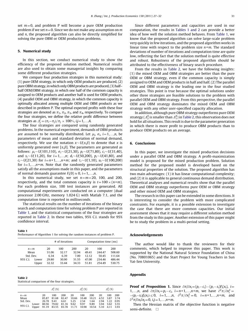
The statistical results on the number of iterations of the binarysearch and computation time for solving problem P are reported inTable 1, and the statistical comparisons of the four strategies arereported in Table 2. In these two tables, 95% C.I. stands for 95%confidence interval.
Table 1Performance of Algorithm 1 for solving the random instances of problem P.
# of iterations Computation time (ms)
n¼m 20 100 200 20 100 200
Mean 31.06 32.17 32.94 49.41 244.47 508.60
Std. Dev. 6.34 6.39 7.00 12.12 50.45 111.64
95% C.I. Lower 29.80 30.90 31.55 47.00 234.46 486.44
Upper 32.32 33.44 34.33 51.81 254.49 530.75
Table 2Statistical comparison of the four strategies.
D41 (%) D4
2 (%) D43 (%)
n¼m 20 100 200 20 100 200 20 100 200Mean 85.87 81.68 82.47 10.66 10.48 10.21 4.52 3.87 3.74Std. Dev. 26.78 9.41 6.61 5.25 2.54 1.64 2.94 1.22 0.95
95% C.I.Lower 80.56 79.82 81.16 9.62 9.97 9.89 3.94 3.62 3.55Upper 91.19 83.55 83.78 11.71 10.98 10.54 5.10 4.11 3.93
Since different parameters and capacities are used in ourcomputation, the results in Tables 1 and 2 can provide a betteridea of how well the solution method behaves. From Table 1, weknow that the proposed algorithm can solve large-scale problemvery quickly in few iterations, and the proposed algorithm works inlinear time with respect to the problem size n+m. The standarddeviations of number of iterations and computation time are quitelow, reflecting the fact that the solution method is quite effectiveand robust. Robustness of the proposed algorithm should beattributed to the effectiveness of binary search procedure.
From the results in Table 2, we have the following insights:(1) the mixed OEM and OBM strategies are better than the pureOEM or OBM strategy, even if the common capacity is simplyassigned to OEM and OEM products in half and half. (2) The parallelOEM and OBM strategy is the leading one in the four studiedstrategies. This point is true because the optimal solutions underother three strategies are feasible solutions to the problem withparallel OEM and OBM strategy. From this perspective, the parallelOEM and OBM strategy dominates the mixed OEM and OBMstrategy with any other user-specified capacity allocation.
In addition, although pure OBM strategy outperforms pure OEMstrategy (D4
2 is smaller thanD41) in Table 2, this observation does not
hold for all situations. This result is due to the parameter generationin which there is more profit to produce OBM products than toproduce OEM products on an average.
6. Conclusions
In this paper, we investigate the mixed production decisionsunder a parallel OEM and OBM strategy. A profit-maximizationmodel is proposed for the mixed production problem. Solutionmethod for the proposed model is developed based on thestructural properties of the solution. The proposed algorithm hastwo main advantages: (1) it has linear computational complexity;and (2) it is applicable to general continuous demand distribution.Theoretical analyses and numerical results show that the parallelOEM and OBM strategy outperforms pure OEM or OBM strategyand other mixed OEM and OBM strategies.
The research in this paper can be extended in some directions. Itis interesting to consider the problem with more complicatedconstraints. For example, it is a possible extension to investigatethe case that there are more common capacities. Our initialassessment shows that it may require a different solution methodfrom the study in this paper. Another extension of this paper mightbe to study the problem in a multi-period setting.
Acknowledgements
The author would like to thank the reviewers for theircomments, which helped to improve this paper. This work issupported by the National Natural Science Foundation of China(No. 70801065) and the Start Project for Young Teachers in SunYat-Sen University.
Appendix
Proof of Proposition 1. Since @p/@xi¼(pi�ci)�(pi�si)Fi(xi), i¼
1,y,n, and @p/@xi¼pi�ci, i¼n+1,y,n+m, we have @2p=@x2i ¼
�ðpi�siÞfiðxiÞr0, i¼1,y,n, @2p=@x2i ¼ 0, i¼n+1,y,n+m, and
q2p/qxiqxj¼0, i,j¼1,y,n+m.
Then the Hessian matrix of the objective function is negative
semi-definite. &
B. Zhang / Int. J. Production Economics 130 (2011) 27–3232
Proof of Proposition 2.
(a)
Note that ~xi ¼minfF�1i ððpi�ciÞ=ðpi�siÞÞ,zig, i¼1,y,n. If zirF�1i
ððpi�ciÞ=ðpi�siÞÞ, i¼1,y,n, then ~xi ¼ zi, and hence theupper bound constraint in Eq. (4) ensures x�i r ~xi; ifzi4F�1
i ððpi�ciÞ=ðpi�siÞÞ, i¼1,y,n, then ~xi ¼ F�1i ððpi�ciÞ=
ðpi�siÞÞ. In this case, if x�i 4 ~xi, then we have @p=@x�i oðpi�ciÞ�ðpi�siÞFið ~xiÞ ¼ 0, and hence a sufficient small decreaseon xi will increase the expected profit. Thus, we have x�i r ~xi,i¼1,y,n. Since ~xi ¼ zi,i¼n+1,y,n+m, then the upper boundconstraint in Eq. (4) ensures x�i r ~xi.P
(b)
The condition nþmi ¼ 1 ti ~xirt implies that the common capacityconstraint is inactive, thus we have x�i ¼ ~xi, i¼1,y,n+m.P P
(c) If nþmi ¼ 1 tix�i ot, then the condition nþm
i ¼ 1 ti ~xi4t implies thatthere exists at least one kA{1,y,n+m} such that x�ko ~xk. If krn,then x�koF�1
k ððpk�ckÞ=ðpk�skÞÞ and x�kozk, we have @p=@x�k ¼
ðpk�ckÞ�ðpk�skÞFkðx�kÞ40; if kZn+1, then we have x�kozk and
@p=@x�k ¼ pk�ck40. Thus, @p=@x�k40, x�kozk, andPnþm
i ¼ 1 tix�i ot
imply that a sufficient small increase on xk will increase theexpected profit. &
Proof of Proposition 3. Note that gi ¼ ðpi�ciÞ=ti for all i¼
1,y,n+m. We first prove the results in Eq. (10). For i¼1,y,n, wewill prove the results in three cases: (1) giol, (2) gi�(pi�si)Fi(zi)/ti4l, and (3) gi�(pi�si)Fi(zi)/tirlrgi.
(1)
If giol, according to Eq. (6), we have wi¼lti�giti+(pi�si)Fi(xi)+vi40, then the slackness condition wixi¼0 in Eq. (8)requires xi(l)¼0.(2)
If gi�(pi�si)Fi(zi)/ti4l, then giti�lti4(pi�si)Fi(zi). According toEq. (6), we have vi¼giti�lti�(pi�si)Fi(xi)+wi40, and theslackness condition vi(zi�xi)¼0 in Eq. (8) implies that xi(l)¼zi.(3)
In the case of gi�(pi�si)Fi(zi)/tirlrgi, we have giti�ltiZ0 and lti�giti+(pi�si)Fi(zi)Z0. We first prove wi¼0 and vi¼0.If wi40, from the slackness condition wixi¼0, we havexi¼0. According to Eq. (6), we have vi¼giti�lti+wi40, andthe slackness condition vi(zi�xi)¼0 implies that xi¼zi, whichviolates xi¼0. If vi40, from the slackness condition vi(zi�xi)¼0, we have xi¼zi. According to Eq. (6), we have wi¼lti�giti
+(pi�si)Fi(zi)+vi40, and the slackness condition wixi¼0implies that xi¼0, which violates xi¼zi. Thus we have wi¼0and vi¼0. Substituting wi¼0 and vi¼0 into Eq. (6), we have(pi�ci)�(pi�si)Fi(xi)�lti¼0, and hence xiðlÞ¼F�1
i ððpi�ci�ltiÞ=
ðpi�siÞÞ.
In the following, we will prove the results of Eq. (11) in three
cases: giol, gi4l, and gi¼l, i¼n+1,y,n+m. If giol, according to
Eq. (7), we have wi¼lti�giti+vi40, and the slackness condition
wixi¼0 implies xi(l)¼0. If gi4l, from Eq. (7), we have vi¼giti
�lti+wi40, and the slackness condition vi(zi�xi)¼0 implies that
xi(l)¼zi. If gi¼l, then from Eq. (7), we know wi¼vi. If wi¼via0,
then the slackness conditions wixi¼0 and vi(zi�xi)¼0 will never be
satisfied simultaneously. Thus, there must be wi¼vi¼0, and hence
xi(l) can take any real value yiA[0,zi]. &
Proof of Proposition 4. SincePnþm
i ¼ 1 ti ~xi4t, according toProposition 2(c), we know that
Pnþmi ¼ 1 tix
�i ¼ t.
Since {k1,y,k2}aF, according toPnþm
i ¼ 1 tix�i ¼ t, we knowGðl�ÞþPk2
i ¼ k1tix�i ðl�Þ ¼ t. Since x�i ðl
�ÞA ½0,zi� for all i¼k1,y,k2, we have
Gðl�ÞrtrGðl�ÞþPk2
i ¼ k1tizi. So there must exist one kA{k1,y,k2}
such that Gðl�ÞþPk�1
k1tizirtrGðl�Þþ
Pki ¼ k1
tizi. From Eq. (14),
we know that x�i ðl�Þ in Eq. (16) satisfies the optimal structures
described in Eq. (11). It is easily verified thatPnþm
i ¼ 1 tix�i ðl�Þ ¼ t
is met. &
References
Abdel-Malek, L., Montanari, R., 2005. An analysis of the multi-product newsboyproblem with a budget constraint. International Journal of Production Econom-ics 97, 296–307.
Abdel-Malek, L., Montanari, R., Morales, L.C., 2004. Exact, approximate, and genericiterative models for the multi-product newsboy with budget constraint.International Journal of Production Economics 91, 189–198.
Chen, G.S., 1989. OEM or OBM. Taiwan Economic Research 134, 44–48.Cheng, J.M.S., Blankson, C., Wu, P.C.S., Chen, S.S.M., 2005. A stage model of
international brand development: the perspectives of manufacturers fromtwo newly industrialized economies—South Korea and Taiwan. IndustrialMarketing Management 34 (5), 504–514.
Chu, W., 2009. Can Taiwan’s second movers upgrade via branding? Research Policy38 1054–1065.
Eng, T.Y., Spickett-Jones, J.G., 2009. An investigation of marketing capabilities andupgrading performance of manufacturers in mainland China and Hong Kong.Journal of World Business 44 (4), 463–475.
Erlebacher, S.J., 2000. Optimal and heuristic solutions for the multi-item news-vendor problem with a single capacity constraint. Production and OperationsManagement 9 (3), 303–318.
Hadley, G., Whitin, T., 1963. Analysis of Inventory Systems. Prentice-Hall, Engle-wood Cliffs, NJ.
Humphrey, J., 2004. Upgrading in global value chains. ILO Policy IntegrationDepartment, Working paper 28, ILO.
Jin, Y., 2008. Experience of design management in Taiwan. China–USA BusinessReview 7 (2), 54–57.
Kabak, I., Weinberg, C., 1972. The generalized newsboy problem, contract negotia-tions and secondary vendors. IIE Transactions 4, 154–157.
Komoto, H., Tomiyama, T., Silvester, S., Brezet, H., 2009 Analyzing supply chainrobustness for OEMs from a life cycle perspective using life cycle simulation.International Journal of Production Economics, doi:10.1016/j.ijpe.2009.11.017.
Lian, S., 2007. Industry environment, OBM strategic choice and new ventureperformance. Master’s Thesis, National Cheng Kung University, Taiwan.
Li, J.Y., 2006. Utilizing fuzzy AHP approach for the critical resource of the OBM–OEMsimultaneous model: an analysis from the resource-based view. Master’s Thesis,Ming Chuan University, Taiwan.
Li, Q.H., 1992. The brand strategy of Taiwanese firms under international environ-ment. Unpublished Master Thesis.
McDougall, P.P., Covin, J.G., Robinson Jr., R.B., Herron, L., 1994. The effects of industrygrowth and strategic breadth on new venture performance and strategycontent. Strategic Management Journal 15 (7), 537–554.
Moon, I., Silver, E., 2000. The multi-item newsvendor problem with a budgetconstraint and fixed ordering costs. Journal of Operational Research Society 51,602–608.
Niederhoff, J.A., 2007. Using separable programming to solve the multi-productmultiple ex-ante constraint newsvendor problem and extensions. EuropeanJournal of Operational Research 176, 941–955.
Tan, J., 2007. Phase transitions and emergence of entrepreneurship: the transforma-tion of Chinese SOEs over time. Journal of Business Venturing 22 (1), 77–96.
Vairaktarakis, G.L., 2000. Robust multi-item newsboy models with a budgetconstraint. International Journal of Production Economics 66, 213–226.
Zhang, B., Du, S., 2010. Multi-product newsboy problem with limited capacity andoutsourcing. European Journal of Operational Research 202, 107–113.
Zhang, B., Hua, Z., 2008. A unified method for the convex nonlinear knapsackproblem. European Journal of Operational Research 191, 1–6.
Zhang, B., Hua, Z., 2010. A portfolio approach to multi-product newsboy problemwith budget constraint. Computers & Industrial Engineering 58, 759–765.
Zhang, B., Xu, X., Hua, Z., 2009. A binary search method for the multi-productnewsboy problem with budget constraint. International Journal of ProductionEconomics 117, 136–141.
Zhang, B., 2010. Capacity-constrained multiple-market price discrimination.Working paper, Sun Yat-Sen University, China.