Optimal placement of active braces by using PSO · PDF fileOptimal placement of active braces by using PSO algorithm ... concrete shear walls and core wall systems. ... The applied

ORIGINAL RESEARCH

Optimal placement of active braces by using PSO algorithmin near- and far-field earthquakes

M. Mastali1 • A. Kheyroddin2,3 • B. Samali4 • R. Vahdani2

Received: 16 February 2015 / Accepted: 1 February 2016 / Published online: 15 February 2016

� The Author(s) 2016. This article is published with open access at Springerlink.com

Abstract One of the most important issues in tall build-

ings is lateral resistance of the load-bearing systems against

applied loads such as earthquake, wind and blast. Dual

systems comprising core wall systems (single or multi-cell

core) and moment-resisting frames are used as resistance

systems in tall buildings. In addition to adequate stiffness

provided by the dual system, most tall buildings may have

to rely on various control systems to reduce the level of

unwanted motions stemming from severe dynamic loads.

One of the main challenges to effectively control the

motion of a structure is limitation in distributing the

required control along the structure height optimally. In

this paper, concrete shear walls are used as secondary

resistance system at three different heights as well as

actuators installed in the braces. The optimal actuator

positions are found by using optimized PSO algorithm as

well as arbitrarily. The control performance of buildings

that are equipped and controlled using the PSO algorithm

method placement is assessed and compared with arbitrary

placement of controllers using both near- and far-field

ground motions of Kobe and Chi–Chi earthquakes.

Keywords Pole assignment method � Near- and far-field

earthquakes � PSO algorithm � Optimal actuator position

Introduction

The rapid growth of the urban population and consequent

pressure on limited space have considerably influenced city

residential development. The high cost of land, the desire

to avoid ongoing urban sprawl, and the need to preserve

important agricultural land have all contributed to drive

residential buildings upward. Nowadays, high-rise build-

ings have become one of the impressive reflections and

icons of today’s civilization. The outlook of cities all over

the world has been changing with these tall and slender

structures (Smith and Coull 1991). Tall buildings use load-

resisting systems against applied lateral loads such as

concrete shear walls and core wall systems. The main

problem of these systems is their limitations in controlling

the response of super tall buildings (Kheyroddin et al.

2014; Keshavarz et al. 2011). Therefore, some strategies

have been used to control and make serviceable tall

buildings in addition to the lateral load-resisting systems

which included: (1) passive control; (2) semi-active con-

trol; (3) active control, or their combinations. In the passive

control, the structure uses its internal energy to dissipate

external energy. A large number of studies have been

conducted on the active control concept (Yang et al. 2004;

Kwok et al. 2006). These systems are able to control the

structure displacements, accelerations and internal forces

by using external energy and providing a direct counter-

acting force by the actuators. Using this strategy for con-

trolling structures against external excitation has

limitations because of some technological and economic

aspects (Symans and Constantinou 1999), as well as the

& M. Mastali

[email protected]; [email protected]

1 Department of Civil Engineering, ISISE, Minho University,

Campus de Azurem, 4800-058 Guimaraes, Portugal

2 Faculty of Civil Engineering, Semnan University, Seman,

Iran

3 Department of Civil Engineering and Applied Mechanics,

University of Texas, Arlington, TX, USA

4 School of Civil and Environmental Engineering, University

of Western Sydney, Sydney, Australia

123

Int J Adv Struct Eng (2016) 8:29–44

DOI 10.1007/s40091-016-0111-3

http://crossmark.crossref.org/dialog/?doi=10.1007/s40091-016-0111-3&domain=pdf

http://crossmark.crossref.org/dialog/?doi=10.1007/s40091-016-0111-3&domain=pdf

risks associated with loss of external power in the event of

a major earthquake or severe wind load. These systems

require high amount of external energy for controlling the

structures in comparison with other strategies. Hence, to

overcome this problem, semi-active control was proposed

as a strategy which compensates for the shortcomings of

active control. In this control method, structural properties

such as damping and/or stiffness are altered by use of

special devices with very little external energy to activate

such systems. As a result, much lower amount of external

energy is required to control the structures during external

excitations and there is a potential in this method to

achieve control levels similar to active systems (Amini and

Vahdani 2008). Because of limitations in the number of

actuators and due to economic reasons, actuator location is

an important issue in control problems. Nowadays,

numerical methods, such as those inspired by nature, are

used in optimizing actuator locations. These methods

include ant colony, genetic algorithm, PSO (particle swarm

optimization) algorithm, etc.

In this paper, three 3D buildings with different heights

are used to investigate the effectiveness of the designed

controller. In these systems, the concrete shear walls were

also considered as the secondary load-resisting system.

In the present study, three structures with 21, 15, and 9

stories were studied, considering 3, 2, and 1 actuator,

respectively. The actuators were placed in the system in

two ways, which include (1) finding the optimized position

of the optimized actuator using the PSO algorithm; (2)

installing an actuator at arbitrary positions. Structures were

modelled in MATLAB software. In this regard, finite ele-

ment method was used for modelling these structures and

the interactions between the frame and walls (Ghali et al.

2003). The obtained stiffness from this method was used in

modelling of structures in MATLAB software. The novelty

of the present paper was using PSO algorithm to optimize

actuator locations.

Analysis of a planar frame in the presence of shearwalls

The contribution of shear walls in a frame depends on the

wall stiffness with respect to other structural elements.

Commonly, it is assumed that horizontal forces are applied

at the floor levels. Moreover, it is assumed that floor

stiffness in the horizontal direction is very high compared

to the stiffness of columns and shear walls. Therefore, it is

assumed that the floors move as rigid bodies in the hori-

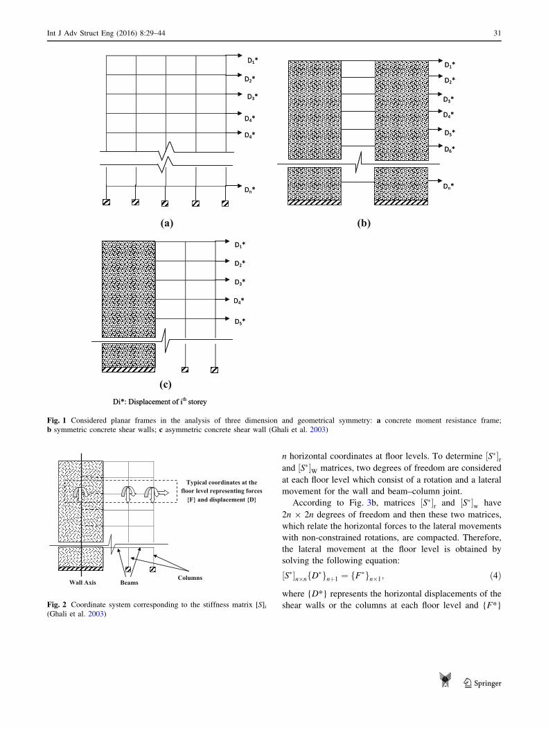
zontal direction. Let us consider the structure shown in

Fig. 1, which is constructed of some parallel frames with

symmetrical axes.

Some of these structures use shear walls as the sec-

ondary load-resisting system. Because of geometric and

loading symmetry, floors move without any rotation. By

assuming rigid body motion for the floors, each level has a

displacement equal to [D*]. The stiffness matrix [S]nxn (n is

the number of stories) corresponding to the coordinate

{D*} for each planar frame is calculated and then all the

stiffness matrices are assembled to obtain the stiffness

matrix of the structure:

½S�� ¼Xm

i¼1

½S��i; ð1Þ

where m is the number of frames. The lateral movement at

the floor level is calculated using the following equation in

which {F} is the applied force vector on each floor level:

½S��n�nfD�gn�1 ¼ fF�gn�1: ð2Þ

Approximate analysis of the planar structures

The shear wall deformations are similar to cantilever

beams. This simplification is reasonable due to the fact that

the rotations are constrained at the ends of the columns by

beams in tension (Ghali et al. 2003). It is obvious that shear

wall moment of inertia, I, is higher than that of the beam

which subsequently leads to reduction in the beam ability

to control rotations caused by deformation of the cantilever

beam at the floor level. The observed behaviour suggests

that the load-resisting systems are composed of two parts;

see Figs. 2 and 3.

They are composed of (1) shear wall system; (2)

equivalent column. Moment of inertia (IW) of the shear

wall and the column (IC) at each floor level is equal to the

sum of moments of inertia of the shear walls and the col-

umns at that floor level. The second system is an equivalent

column which is connected to the beams in a rigid way.

Additionally, it is obvious that these two load-resisting

systems are connected to each other by non-deformable

tension elements and that all the external forces are applied

at the floor level. Axial deformations in all structural ele-

ments are neglected, while shear deformations in walls and

columns can be considered or neglected in the analysis. In

case the shear deformations are considered, the effective

(reduced) area is equal to the sum of the reduced areas of

the walls and the columns at each floor level. It is assumed

that the idealized structure has n degrees of freedom, rep-

resenting the lateral movements of the floors. The stiffness

matrix of the structure S�n�n

� �is obtained by summing the

stiffness matrices of the two resisting systems:

½S�� ¼ ½S��w þ ½S��r; ð3Þ

where S�½ �r and S�½ �W are the stiffness matrices of the

resisting frame and the wall, respectively, corresponding to

30 Int J Adv Struct Eng (2016) 8:29–44

123

n horizontal coordinates at floor levels. To determine S�½ �rand S�½ �W matrices, two degrees of freedom are considered

at each floor level which consist of a rotation and a lateral

movement for the wall and beam–column joint.

According to Fig. 3b, matrices S�½ �r and S�½ �w have

2n 9 2n degrees of freedom and then these two matrices,

which relate the horizontal forces to the lateral movements

with non-constrained rotations, are compacted. Therefore,

the lateral movement at the floor level is obtained by

solving the following equation:

½S��n�nfD�gnþ1 ¼ fF�gn�1; ð4Þ

where {D*} represents the horizontal displacements of the

shear walls or the columns at each floor level and {F*}

(a) (b)

(c) Di*: Displacement of iDi*: Displacement of ithth storey storey

DD11* *

DD22* *

DD33* *

DD44* *

DD44* *

DDnn* *

DD11* *

DD22* *

DD33* *

DD55* *

DD66* *

DDnn* *

DD44* *

DD11* *

DD22* *

DD33* *

DD44* *

DD55* *

Fig. 1 Considered planar frames in the analysis of three dimension and geometrical symmetry: a concrete moment resistance frame;

b symmetric concrete shear walls; c asymmetric concrete shear wall (Ghali et al. 2003)

Wall Axis Columns

Beams

Typical coordinates at the floor level representing forces

{F} and displacement {D}

Fig. 2 Coordinate system corresponding to the stiffness matrix [S]i(Ghali et al. 2003)

Int J Adv Struct Eng (2016) 8:29–44 31

123

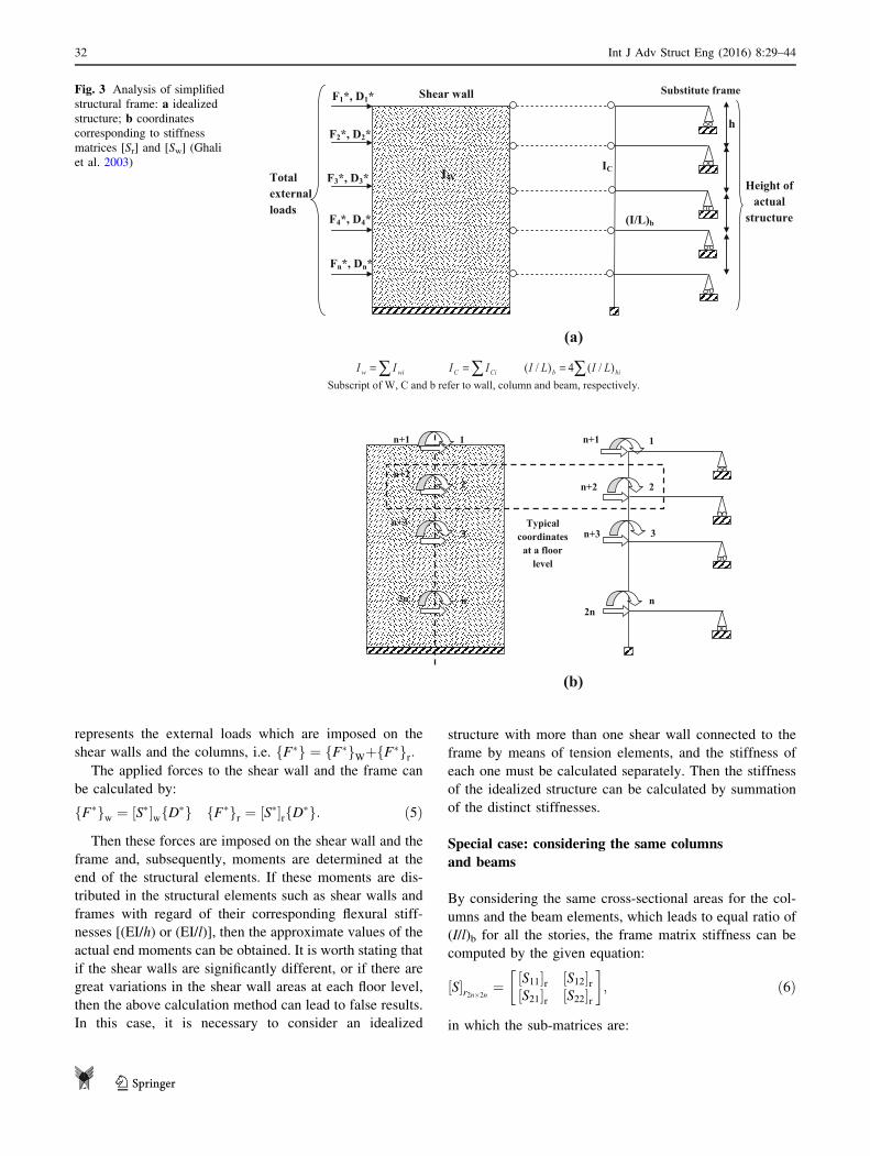
represents the external loads which are imposed on the

shear walls and the columns, i.e. F�f g ¼ F�f gWþ F�f gr:The applied forces to the shear wall and the frame can

be calculated by:

fF�gw ¼ ½S��wfD�g fF�gr ¼ ½S��rfD�g: ð5Þ

Then these forces are imposed on the shear wall and the

frame and, subsequently, moments are determined at the

end of the structural elements. If these moments are dis-

tributed in the structural elements such as shear walls and

frames with regard of their corresponding flexural stiff-

nesses [(EI/h) or (EI/l)], then the approximate values of the

actual end moments can be obtained. It is worth stating that

if the shear walls are significantly different, or if there are

great variations in the shear wall areas at each floor level,

then the above calculation method can lead to false results.

In this case, it is necessary to consider an idealized

structure with more than one shear wall connected to the

frame by means of tension elements, and the stiffness of

each one must be calculated separately. Then the stiffness

of the idealized structure can be calculated by summation

of the distinct stiffnesses.

Special case: considering the same columns

and beams

By considering the same cross-sectional areas for the col-

umns and the beam elements, which leads to equal ratio of

(I/l)b for all the stories, the frame matrix stiffness can be

computed by the given equation:

½S�r2n�2n¼ ½S11�r ½S12�r

½S21�r ½S22�r

� �; ð6Þ

in which the sub-matrices are:

(a)

∑= wiw II ∑= CiC II ∑= bib LILI )/(4)/(Subscript of W, C and b refer to wall, column and beam, respectively.

(b)

IWIC

h

F1*, D1*

F2*, D2*

F3*, D3*

F4*, D4*

Fn*, Dn*

(I/L)b

Shear wall

Height of actual

structure

Total external loads

Substitute frame

1

2

3

n

n+1

n+2

n+3

2n

1

2

3

n 2n

n+3

n+2

n+1

Typical coordinates

at a floor level

Fig. 3 Analysis of simplified

structural frame: a idealized

structure; b coordinates

corresponding to stiffness

matrices [Sr] and [Sw] (Ghali

et al. 2003)


123

½S11�r ¼2ðSþ tÞ

h2:

1 �1 0 0 0 0 0 0

�1 2 �1 0 0 0 0 0

0 : 2 : 0 0 0 0

0 0 : : : 0 0 0

0 0 0 : : : 0 0

0 0 0 0 : 2 �1 0

0 0 0 0 0 �1 2 �1

0 0 0 0 0 0 �1 2

2

66666666664

3

77777777775

n�n

;

ð7Þ

½S21�r ¼ ½S12�Tr

¼ ðSþ tÞh

�1 1 0 0 0 0 0 0

�1 0 1 0 0 0 0 0

0 �1 0 1 0 0 0 0

0 0 : : : 0 0 0

0 0 0 : : : 0 0

0 0 0 0 : : : 0

0 0 0 0 0 �1 0 1

0 0 0 0 0 0 �1 0

2

66666666664

3

77777777775

n�n

;

ð8Þ

½S22�r¼S

ð1þbÞ c 0 0 0 0 0 0

c ð2þbÞ c 0 0 0 0 0

0 c ð2þbÞ c 0 0 0 0

0 0 c : : 0 0 0

0 0 0 : : : 0 0

0 0 0 0 : : : 0

0 0 0 0 0 c ð2þbÞ c

0 0 0 0 0 0 c ð2þbÞ

2

66666666664

3

77777777775

n�n

;

ð9Þ

where:

b ¼ 3E

SI=L

� �

bS ¼ ð4þ aÞ

ð1þ aÞEIc

ht ¼ ð2� aÞ

ð1þ aÞEIc

h

c ¼ p t=S�

;ð10Þ

In which S is the rotational stiffness of a column when

the support is clamped; t is the transferred moment and c is

the transferred coefficient. The shear deformation of the

vertical elements can be calculated by:

a ¼ 12EIc

h2Garcð11Þ

and the shear deformation of the beams are neglected. The

effective cross-sectional area of the columns is computed

by adding all the effective cross-sectional areas of the

columns (arc ¼P

arci).

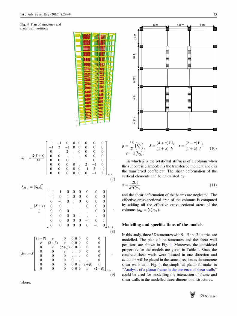
Modelling and specifications of the models

In this study, three 3D structures with 9, 15 and 21 stories are

modelled. The plan of the structures and the shear wall

positions are shown in Fig. 4. Moreover, the considered

properties for the models are given in Table 1. Since the

concrete shear walls were located in one direction and

actuators will be placed in the same direction as the concrete

shear walls as in Fig. 4, the simplified planar formulas in

‘‘Analysis of a planar frame in the presence of shear walls’’

could be used for modelling the interaction of frame and

shear walls in the modelled three-dimensional structures.

6 m

6 m6 m

6 m

m8.

4m

8.4

m8.

4

4.8 mFig. 4 Plan of structures and

shear wall positions


123

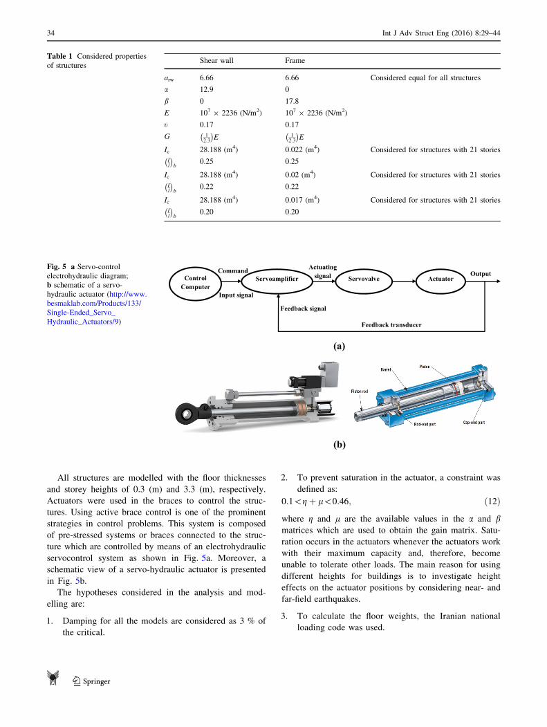
All structures are modelled with the floor thicknesses

and storey heights of 0.3 (m) and 3.3 (m), respectively.

Actuators were used in the braces to control the struc-

tures. Using active brace control is one of the prominent

strategies in control problems. This system is composed

of pre-stressed systems or braces connected to the struc-

ture which are controlled by means of an electrohydraulic

servocontrol system as shown in Fig. 5a. Moreover, a

schematic view of a servo-hydraulic actuator is presented

in Fig. 5b.

The hypotheses considered in the analysis and mod-

elling are:

1. Damping for all the models are considered as 3 % of

the critical.

2. To prevent saturation in the actuator, a constraint was

defined as:

0:1\gþ l\0:46; ð12Þ

where g and l are the available values in the a and bmatrices which are used to obtain the gain matrix. Satu-

ration occurs in the actuators whenever the actuators work

with their maximum capacity and, therefore, become

unable to tolerate other loads. The main reason for using

different heights for buildings is to investigate height

effects on the actuator positions by considering near- and

far-field earthquakes.

3. To calculate the floor weights, the Iranian national

loading code was used.

Table 1 Considered properties

of structuresShear wall Frame

arw 6.66 6.66 Considered equal for all structures

a 12.9 0

b 0 17.8

E 107 9 2236 (N/m2) 107 9 2236 (N/m2)

t 0.17 0.17

G 12:3

� E 1

2:3

� E

Ic 28.188 (m4) 0.022 (m4) Considered for structures with 21 stories

Il

� b

0.25 0.25


Il

� b

0.22 0.22


Il

� b

0.20 0.20

(a)

(b)

Control Computer

t

Servoamplifier Servovalve Actuator Command

Input signal

Actuating signal Output

Feedback transducer

Feedback signal

Fig. 5 a Servo-control

electrohydraulic diagram;

b schematic of a servo-

hydraulic actuator (http://www.

besmaklab.com/Products/133/

Single-Ended_Servo_

Hydraulic_Actuators/9)


123

http://www.besmaklab.com/Products/133/Single-Ended_Servo_Hydraulic_Actuators/9




The Chi–Chi and Kobe records as both near- and far-

field ground motions were used to analyse models listed in

Table 2 (http://peer.berkeley.edu/products/strong_ground_

motion_db.html).

Properties of near- and far-field earthquakes

Obviously, there are some differences in the properties

of near- and far-field earthquakes. Therefore, it seems

necessary to investigate the effects of these differences

on the buildings and to classify these effects. A distance

shorter than 15 km from a fault line is referred to as

near-fault zone; otherwise, it is known as far-field zone.

In the near-field zone, earthquake effects depend on

three main factors, namely (1) rupture mechanism; (2)

rupture propagation directions with respect to the site,

and (3) permanent displacement due to fault slippage.

These factors create two phenomena, which are rupture

directivity and step fling. Rupture directivity is also

divided into two phenomena, which are forward direc-

tivity and backward directivity. Forward directivity

effects lead to horizontal oscillations in the direction

perpendicular to the fault line in the form of a horizontal

pulse, which has much more significant effects on the

structures in comparison with a parallel pulse to the fault

line. These pulses lead to an increase in the nonlinear

deformation demands of the structures. Near-fault

ground motions have short duration with high amplitude

and high to medium oscillation periods (International

Institute of Earthquake Engineering and Seismology

2007; Alavi 2001; Galal and Ghobarah 2006; Stewart

et al. 2001). The recorded databases of Kobe and Chi–

Chi earthquakes were used to analyse the structures.

Regard of FEMA 356, the geotechnical specifications

should be taken into account in selection process of the

earthquake record databases (Federal Emergency Man-

agement Agency 2000). Therefore, the frequency con-

tents, spectrum, effective duration, and type of soil could

be varied regard of construction site (Federal Emergency

Management Agency 2000).

Pole Assignment controller design

In this study, Pole Assignment was used as the control

method. The equation of motion of a multi-degree-of-

freedom (MDOF) system by considering a force control

under the effect of a specific excitation is:

½M� €X þ ½C� _X þ ½K�fXg ¼ �½M�fIg €Xg � fUCg; ð13Þ

where {Uc} is the control force vector which has a

dimension equal to that of the displacement vector (n 9 1).

The negative sign on the right hand side of Eq. (13) shows

that the applied force control is in the same direction with

the formed internal resistance due to damping and stiffness

of the structure. [M], [C] and [K] are the mass, damping

and stiffness matrices, respectively, and have the dimen-

sions of (n 9 n). In Eq. (13), {I} is the unit vector with the

dimension of (n 9 1) and xg is the earthquake acceleration

record. By transforming the equation of motion into state-

space, Eq. (13) can be rewritten in the following form:

f _qg ¼ ½A�fqg þ ½Be�€xg þ ½BU�fucg; ð14Þ

where [A] is the system matrix, [Bu] the actuator position

matrix, [Be] the vector of external excitation position and

{q} the space vector. These matrices and vectors are given

by:

½BU� ¼0

�M�1

� �½Be� ¼

0

�I

�;

q ¼x

_x

�½A� ¼

0 I

�M�1K �M�1C

� �:

ð15Þ

The force control Uc is obtained by multiplying the gain

matrix in the space vector:

fUCg ¼ ½F�f q g: ð16Þ

The gain matrix is replaced by:

F ¼ ½FK;FC� ; ð17Þ

where Fk and FC are the stiffness and damping type of

matrices with dimensions of (n 9 n). These components

can be obtained by the following equations:

Table 2 Nominated modelsName Storey number No of actuators Method used for placement of actuators

M21-3-P 21 3 Optimization by using the PSO algorithm



M21-3-A 21 3 Arbitrary




123

http://peer.berkeley.edu/products/strong_ground_motion_db.html

http://peer.berkeley.edu/products/strong_ground_motion_db.html

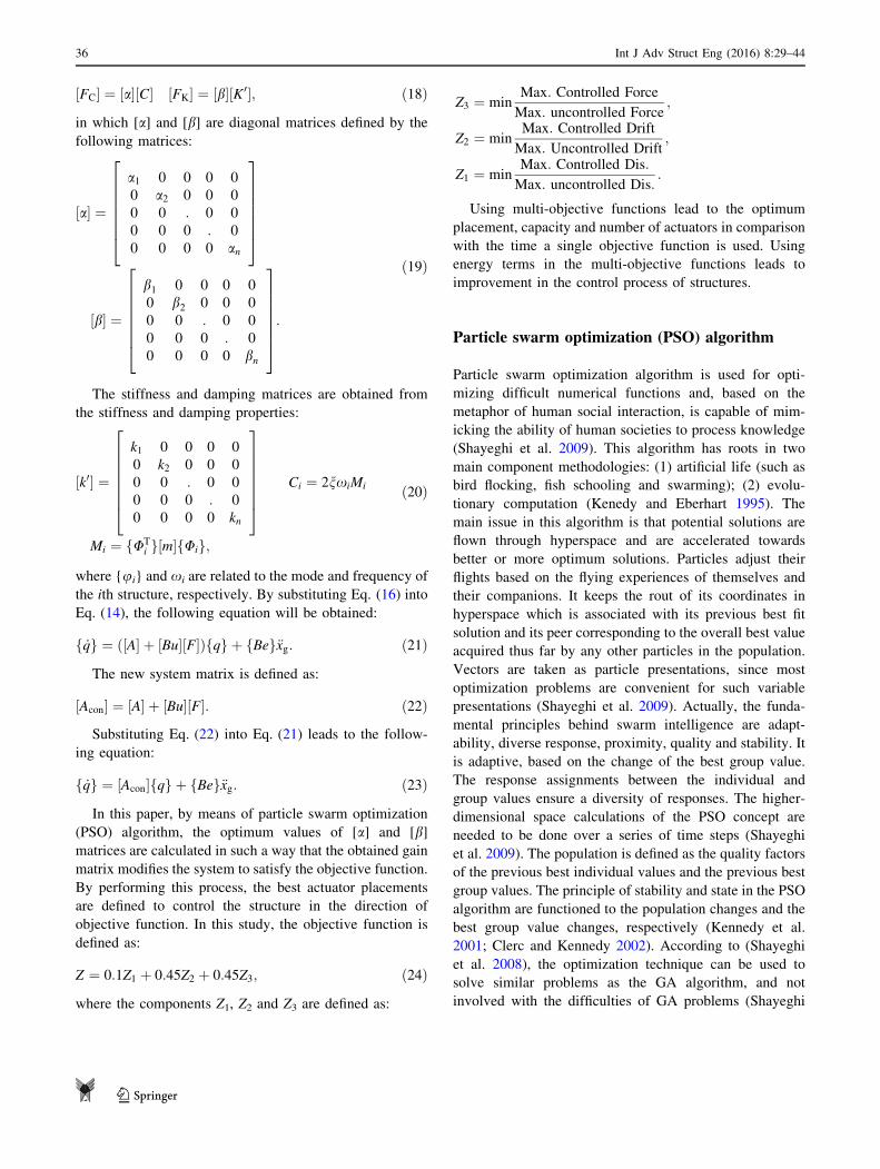
½FC� ¼ ½a�½C� ½FK� ¼ ½b�½K 0�; ð18Þ

in which [a] and [b] are diagonal matrices defined by the

following matrices:

½a� ¼

26666664

a1 0 0 0 0

0 a2 0 0 0

0 0 : 0 0

0 0 0 : 0

0 0 0 0 an

37777775

½b� ¼

2

6666664

b1 0 0 0 0

0 b2 0 0 0

0 0 : 0 0

0 0 0 : 0

0 0 0 0 bn

3

7777775:

ð19Þ

The stiffness and damping matrices are obtained from

the stiffness and damping properties:

½k0� ¼

2

6666664

k1 0 0 0 0

0 k2 0 0 0

0 0 : 0 0

0 0 0 : 0

0 0 0 0 kn

3

7777775Ci ¼ 2nxiMi

Mi ¼ fUTi g½m�fUig;

ð20Þ

where {ui} and xi are related to the mode and frequency of

the ith structure, respectively. By substituting Eq. (16) into

Eq. (14), the following equation will be obtained:

f _qg ¼ ð½A� þ ½Bu�½F�Þfqg þ fBeg€xg: ð21Þ

The new system matrix is defined as:

½Acon� ¼ ½A� þ ½Bu�½F�: ð22Þ

Substituting Eq. (22) into Eq. (21) leads to the follow-

ing equation:

f _qg ¼ ½Acon�fqg þ fBeg€xg: ð23Þ

In this paper, by means of particle swarm optimization

(PSO) algorithm, the optimum values of [a] and [b]matrices are calculated in such a way that the obtained gain

matrix modifies the system to satisfy the objective function.

By performing this process, the best actuator placements

are defined to control the structure in the direction of

objective function. In this study, the objective function is

defined as:

Z ¼ 0:1Z1 þ 0:45Z2 þ 0:45Z3; ð24Þ

where the components Z1, Z2 and Z3 are defined as:

Z3 ¼ minMax: Controlled Force

Max: uncontrolled Force;

Z2 ¼ minMax: Controlled Drift

Max: Uncontrolled Drift;

Z1 ¼ minMax: Controlled Dis:

Max: uncontrolled Dis::

Using multi-objective functions lead to the optimum

placement, capacity and number of actuators in comparison

with the time a single objective function is used. Using

energy terms in the multi-objective functions leads to

improvement in the control process of structures.

Particle swarm optimization (PSO) algorithm

Particle swarm optimization algorithm is used for opti-

mizing difficult numerical functions and, based on the

metaphor of human social interaction, is capable of mim-

icking the ability of human societies to process knowledge

(Shayeghi et al. 2009). This algorithm has roots in two

main component methodologies: (1) artificial life (such as

bird flocking, fish schooling and swarming); (2) evolu-

tionary computation (Kenedy and Eberhart 1995). The

main issue in this algorithm is that potential solutions are

flown through hyperspace and are accelerated towards

better or more optimum solutions. Particles adjust their

flights based on the flying experiences of themselves and

their companions. It keeps the rout of its coordinates in

hyperspace which is associated with its previous best fit

solution and its peer corresponding to the overall best value

acquired thus far by any other particles in the population.

Vectors are taken as particle presentations, since most

optimization problems are convenient for such variable

presentations (Shayeghi et al. 2009). Actually, the funda-

mental principles behind swarm intelligence are adapt-

ability, diverse response, proximity, quality and stability. It

is adaptive, based on the change of the best group value.

The response assignments between the individual and

group values ensure a diversity of responses. The higher-

dimensional space calculations of the PSO concept are

needed to be done over a series of time steps (Shayeghi

et al. 2009). The population is defined as the quality factors

of the previous best individual values and the previous best

group values. The principle of stability and state in the PSO

algorithm are functioned to the population changes and the

best group value changes, respectively (Kennedy et al.

2001; Clerc and Kennedy 2002). According to (Shayeghi

et al. 2008), the optimization technique can be used to

solve similar problems as the GA algorithm, and not

involved with the difficulties of GA problems (Shayeghi


123

et al. 2008). By observing the obtained results from the

analysed problems solved by the PSO algorithm, it was

found that it was robust in solving problems featuring

nonlinearity, non-differentiability and high dimensionality.

The PSO algorithm is the search method to improve the

speed of convergence and find the global optimum value of

the fitness function (Shayeghi et al. 2009).

PSO begins with a population of random solutions

‘‘particles’’ in a D-dimension space. The ith particle is

represented by Xi = (xi1, xi2,…,xiD) (Shayeghi et al.

2009). Each particle keeps the rout coordinates in hyper-

space, associated with the fittest solution. The value of the

fitness for particle ith (pbest) is also stored as Pi = (pi1,

pi2,…,piD). The PSO algorithm keeps rout to approach the

overall best value (gbest), and its location, obtained thus far

by any particle in the population. The PSO algorithm

consists of a step, involving changing the velocity of each

particle towards its pbest and gbest according to Eq. (25).

The velocity of particle i is represented as Vi = (vi1, vi2…viD). Acceleration is weighted by a random term, with

separate random numbers being generated for acceleration

towards pbest and gbest values. Then, the ith particle

position is updated based on Eq. 26 (Kennedy et al. 2001):

viðtÞ ¼ / viðt � 1Þ þ r1c1ðx~pbest � x~iÞ þ r2c2ðx~gbest � x~iÞ;ð25Þ

x~iðtÞ ¼ x~iðt � 1Þ þ v~iðtÞ; ð26Þ

where C1 and C2 are acceleration coefficients. Kenedy

showed that to ensure a stabilized solution, the sum of

these coefficients must be less than 4; otherwise, velocity

and particle positions tend to infinity (Clerc and Kennedy

2002). / represents the inertia weights for which the fol-

lowing equation must be satisfied:

/i0:5ðC1 þ C2Þ � 1: ð27Þ

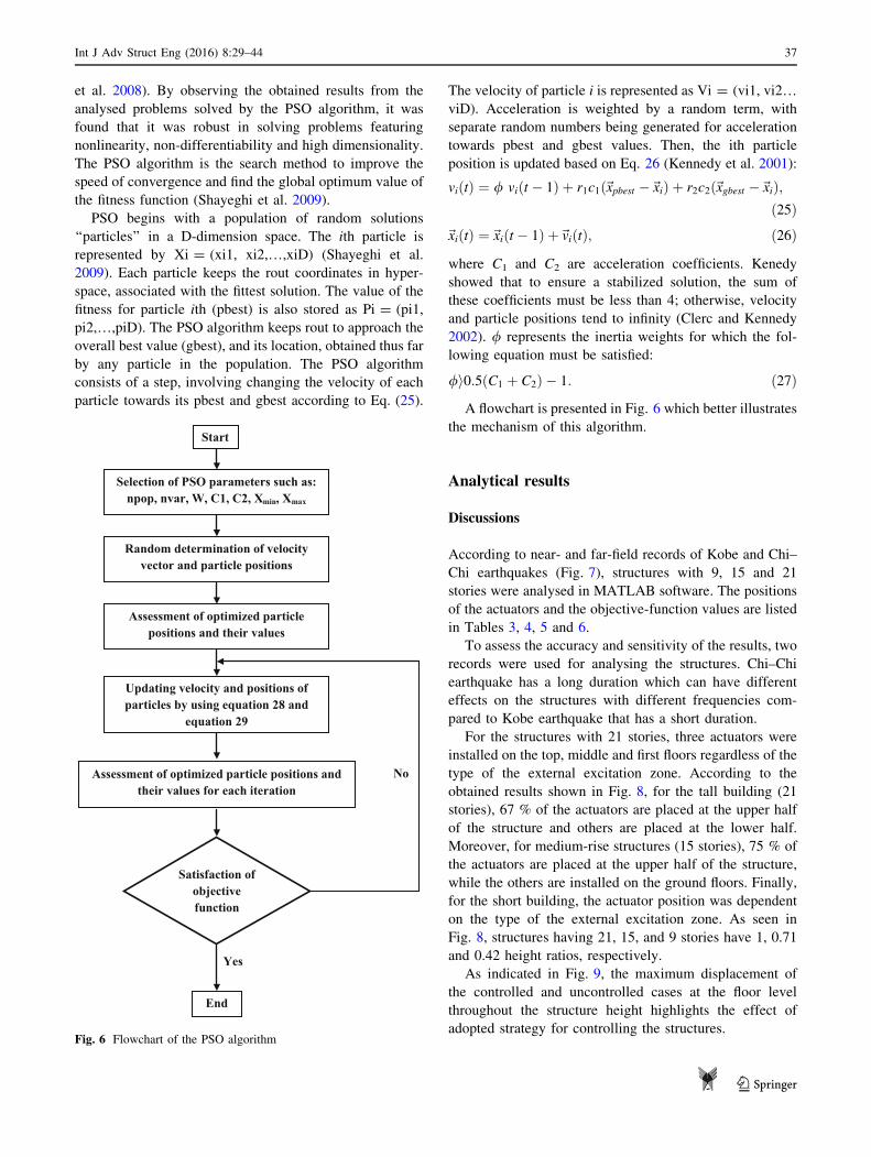
A flowchart is presented in Fig. 6 which better illustrates

the mechanism of this algorithm.

Analytical results

Discussions

According to near- and far-field records of Kobe and Chi–

Chi earthquakes (Fig. 7), structures with 9, 15 and 21

stories were analysed in MATLAB software. The positions

of the actuators and the objective-function values are listed

in Tables 3, 4, 5 and 6.

To assess the accuracy and sensitivity of the results, two

records were used for analysing the structures. Chi–Chi

earthquake has a long duration which can have different

effects on the structures with different frequencies com-

pared to Kobe earthquake that has a short duration.

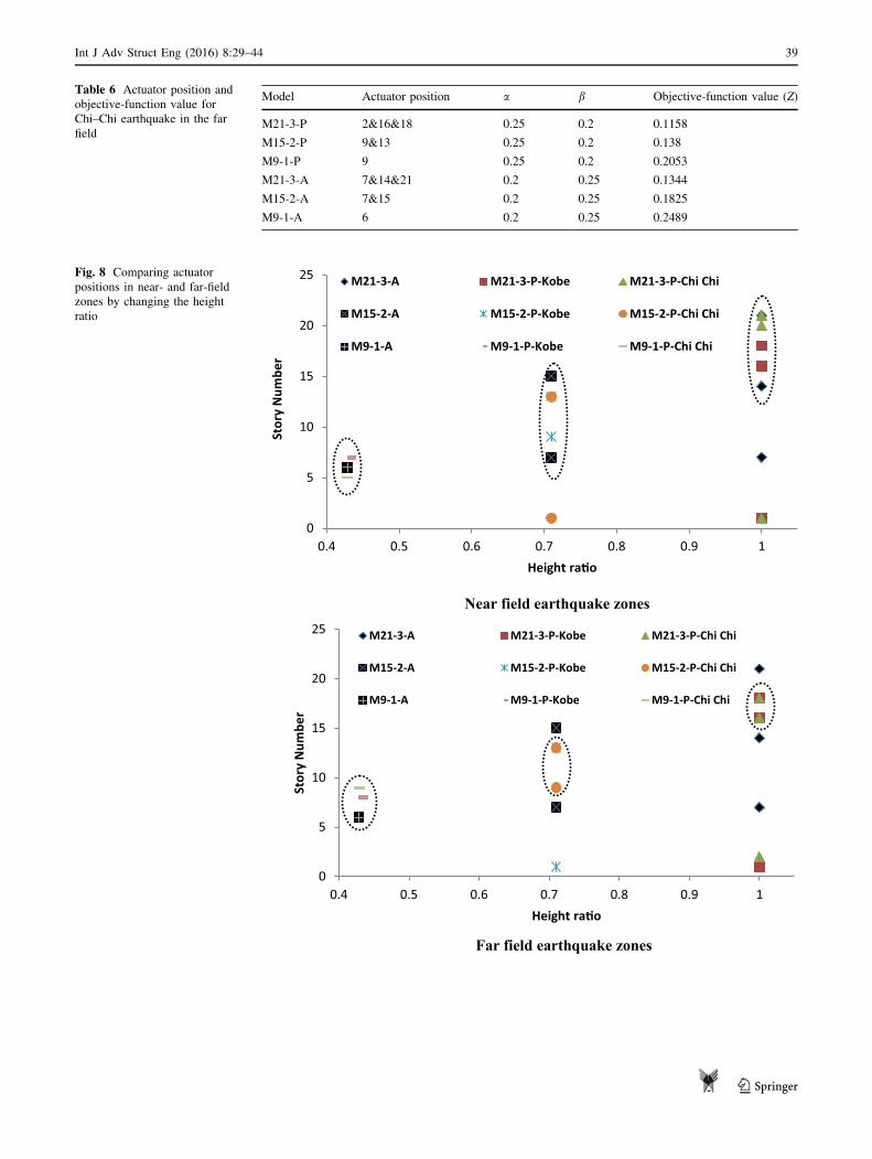
For the structures with 21 stories, three actuators were

installed on the top, middle and first floors regardless of the

type of the external excitation zone. According to the

obtained results shown in Fig. 8, for the tall building (21

stories), 67 % of the actuators are placed at the upper half

of the structure and others are placed at the lower half.

Moreover, for medium-rise structures (15 stories), 75 % of

the actuators are placed at the upper half of the structure,

while the others are installed on the ground floors. Finally,

for the short building, the actuator position was dependent

on the type of the external excitation zone. As seen in

Fig. 8, structures having 21, 15, and 9 stories have 1, 0.71

and 0.42 height ratios, respectively.

As indicated in Fig. 9, the maximum displacement of

the controlled and uncontrolled cases at the floor level

throughout the structure height highlights the effect of

adopted strategy for controlling the structures.

Start

Selection of PSO parameters such as: npop, nvar, W, C1, C2, Xmin, Xmax

Random determination of velocity vector and particle positions

Assessment of optimized particle positions and their values

Updating velocity and positions of particles by using equation 28 and

equation 29

Assessment of optimized particle positions and their values for each iteration

End

No

Yes

Satisfaction of objective function

Fig. 6 Flowchart of the PSO algorithm


123

(a) Far field record of Chi-Chi earthquake (b) Near field record of Chi-Chi earthquake

(c) Far field record of Kobe earthquake (d) Near field record of Kobe earthquake

-0.50

-0.30

-0.10

0.10

0.30

0.50

0 20 40 60 80 100

Acce

lera

�on

(g)

kobe-nf

-0.50

-0.30

-0.10

0.10

0.30

0.50

0 20 40 60 80 100

Acce

lera

�on

(g)

kobe-ff

-0.50

-0.30

-0.10

0.10

0.30

0.50

0 20 40 60 80 100

Acce

lera

�on

(g)

-0.50

-0.30

-0.10

0.10

0.30

0.50

0 20 40 60 80 100

Acce

lera

�on

(g)

Chi-Chi - ff Chi-Chi - nf

Fig. 7 Records of Chi–Chi and Kobe earthquake in both near and far field

Table 3 Actuator position and

objective-function value for

Kobe earthquake in the near

field

Model Actuator position a b Objective function value (Z)

M21-3-P 1&16&18 0.25 0.2 0.1218

M15-2-P 9&13 0.25 0.2 0.1451

M9-1-P 7 0.25 0.2 0.2085

M21-3-A 7&14&21 0.2 0.25 0.1488

M15-2-A 7&15 0.2 0.25 0.1911

M9-1-A 6 0.2 0.25 0.2304



Kobe earthquake in the far field

Model Actuator position a b Objective-function value (Z)

M21-3-P 1&16&18 0.25 0.2 0.1123

M15-2-P 1&13 0.25 0.2 0.2263

M9-1-P 8 0.25 0.2 0.2024

M21-3-A 7&14&21 0.2 0.25 0.1252

M15-2-A 7&15 0.2 0.25 0.2468

M9-1-A 6 0.2 0.25 0.2415



Chi–Chi earthquake in the near

field


M21-3-P 1&20&21 0.25 0.2 0.1101

M15-2-P 1&13 0.25 0.2 0.1804

M9-1-P 5 0.25 0.2 0.3187

M21-3-A 7&14&21 0.2 0.25 0.1257

M15-2-A 7&15 0.2 0.25 0.2043

M9-1-A 6 0.2 0.25 0.315


123

Near field earthquake zones

Far field earthquake zones

0

5

10

15

20

25

0.4 0.5 0.6 0.7 0.8 0.9 1

Stor

y N

umbe

r

Height ra�o

M21-3-A M21-3-P-Kobe M21-3-P-Chi Chi



0

5

10

15

20

25

0.4 0.5 0.6 0.7 0.8 0.9 1

Stor

y N

umbe

r

Height ra�o




Fig. 8 Comparing actuator

positions in near- and far-field

zones by changing the height

ratio



Chi–Chi earthquake in the far

field


M21-3-P 2&16&18 0.25 0.2 0.1158

M15-2-P 9&13 0.25 0.2 0.138

M9-1-P 9 0.25 0.2 0.2053

M21-3-A 7&14&21 0.2 0.25 0.1344

M15-2-A 7&15 0.2 0.25 0.1825

M9-1-A 6 0.2 0.25 0.2489


123

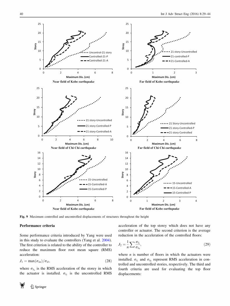
Performance criteria

Some performance criteria introduced by Yang were used

in this study to evaluate the controllers (Yang et al. 2004).

The first criterion is related to the ability of the controller to

reduce the maximum floor root mean square (RMS)

acceleration:

J1 ¼ maxðr€xnÞ=r€xl; ð28Þ

where r€xn is the RMS acceleration of the storey in which

the actuator is installed. r€xl is the uncontrolled RMS

acceleration of the top storey which does not have any

controller or actuator. The second criterion is the average

reduction in the acceleration of the controlled floors:

J2 ¼1

n

X r€xir€x0

; ð29Þ

where n is number of floors in which the actuators were

installed. r€xi and r€x0 represent RMS acceleration in con-

trolled and uncontrolled stories, respectively. The third and

fourth criteria are used for evaluating the top floor

displacements:

Near field of Kobe earthquake Far field of Kobe earthquake

Near field of Chi Chi earthquake Far field of Chi Chi earthquake


0

5

10

15

20

25

0 2 4 6 8

Stor

y

Maximum Dis. (cm)

Uncontrol-21 storyControlled-21-PControlled-21-A

0

5

10

15

20

25

0 1 2 3

Stro

y

Maximum Dis. (cm)

21 story-Uncontrolled

21-controlled-P

21-Controlled-A

0

5

10

15

20

25

0 2 4 6 8 10

Stro

y

Maximum Dis. (cm)


21 story-Controlled-P

21 story-Controlled-A

0

5

10

15

20

25

0 2 4 6 8

Stor

y

Maximum Dis. (cm)

21 Story-Uncontrolled


21 story-Controlled

0

2

4

6

8

10

12

14

16

0 2 4 6 8

Stor

y

Maximum Dis. (cm)

15-Uncontrolled

15-Controlled-A

15-Controlled-P

0

2

4

6

8

10

12

14

16

0 1 2 3 4

Stor

y

Maximum Dis. (cm)

15-Uncontrolled

15-Controlled-A

15-Controlled-P

Fig. 9 Maximum controlled and uncontrolled displacements of structures throughout the height


123

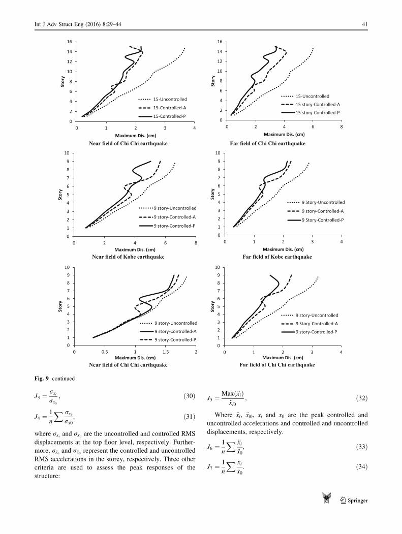
J3 ¼rxlrx0

; ð30Þ

J4 ¼1

n

X rxirx0

; ð31Þ

where rxi and rx0 are the uncontrolled and controlled RMS

displacements at the top floor level, respectively. Further-

more, r€xi and r€x0 represent the controlled and uncontrolled

RMS accelerations in the storey, respectively. Three other

criteria are used to assess the peak responses of the

structure:

J5 ¼Maxð€xiÞ

€xl0; ð32Þ

Where €xl, €xl0, xi and x0 are the peak controlled and

uncontrolled accelerations and controlled and uncontrolled

displacements, respectively.

J6 ¼1

n

X €xi€x0; ð33Þ

J7 ¼1

n

X xi

x0: ð34Þ




0

2

4

6

8

10

12

14

16

0 1 2 3 4

Stor

y

Maximum Dis. (cm)

15-Uncontrolled

15-Controlled-A

15-Controlled-P0

2

4

6

8

10

12

14

16

0 2 4 6 8

Stor

y

Maximum Dis. (cm)

15-Uncontrolled



0

1

2

3

4

5

6

7

8

9

10

0 2 4 6 8

Stor

y

Maximum Dis. (cm)




0

1

2

3

4

5

6

7

8

9

10

0 1 2 3 4

Stor

y

Maximum Dis. (cm)

9 Story-Uncontrolled


9 Story-Controlled-P

0

1

2

3

4

5

6

7

8

9

10

0 0.5 1 1.5 2

Stor

y

Maximum Dis. (cm)



9 story-Controlled-P0

1

2

3

4

5

6

7

8

9

10

0 1 2 3 4

Stor

y

Maximum Dis. (cm)


9 Story-Controlled-A


Fig. 9 continued


123

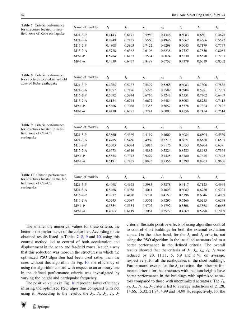
The smaller the numerical values for these criteria, the

better is the performance of the controller. According to the

obtained results listed in Tables 7, 8, 9 and 10, using this

control method led to control of both acceleration and

displacement in the near- and far-field zones in such a way

that this reduction was more in the structures in which the

optimized PSO algorithm had been used rather than the

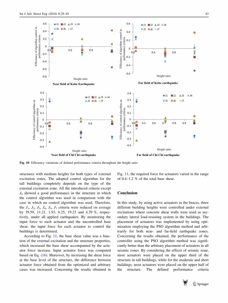
ones without this algorithm. In Fig. 10, the efficiency of

using the algorithm control with respect to an arbitrary one

in the defined performance criteria was investigated by

varying the height and earthquake frequency.

The positive values in Fig. 10 represent lower efficiency

in using the optimized PSO algorithm compared with not

using it. According to the results, the J3, J4, J2, J6, J7

criteria illustrate positive effects of using algorithm control

to control short buildings for both the external excitation

zones. On the other hand, for the J1 and J5 criteria, not

using the PSO algorithm in the installed actuators led to a

better performance in the defined criteria. The overall

results showed that the criteria of J3, J4, J6, J7, J2 were

reduced by 20, 11.11, 5, 5.9 and 5 %, on average,

respectively, for all the earthquakes in the short buildings.

Furthermore, except for the J3 criterion, the other perfor-

mance criteria for the structures with medium heights have

better performance in the buildings with optimized actua-

tors compared to those with unoptimized actuators. The J1,

J2, J4, J5, J6, J7 criteria led to average reductions of 21.28,

14.66, 15.32, 21.74, 4.99 and 14.99 %, respectively, for the

Table 7 Criteria performance

for structures located in near-

field zone of Kobe earthquake

Name of models J1 J2 J3 J4 J5 J6 J7

M21-3-P 0.4143 0.6171 0.5950 0.4346 0.5083 0.6501 0.4678

M21-3-A 0.9249 0.7135 0.5560 0.4946 0.5667 0.4566 0.5572

M15-2-P 0.4808 0.5803 0.7422 0.6298 0.6045 0.7179 0.7777

M15-2-A 0.5728 0.6362 0.6196 0.6238 0.7727 0.7850 0.8083

M9-1-P 0.5784 0.6133 0.7534 0.6024 0.5230 0.5570 0.7797

M9-1-A 0.4339 0.6437 0.8487 0.6752 0.4379 0.6519 0.8532


for structures located in far-field

zone of Kobe earthquake


M21-3-P 0.4064 0.5737 0.5479 0.5268 0.6083 0.7306 0.7838

M21-3-A 0.8657 0.7176 0.5293 0.5589 0.6904 0.5281 0.7237

M15-2-P 0.5092 0.5944 0.6716 0.5243 0.5551 0.7762 0.6407

M15-2-A 0.6134 0.6744 0.6672 0.6484 0.8003 0.8258 0.7413

M9-1-P 0.5666 0.7088 0.7355 0.5657 0.5578 0.7324 0.7122

M9-1-A 0.4430 0.6891 0.7741 0.6003 0.4556 0.7154 0.7514


for structures located in near-

field zone of Chi–Chi

earthquake


M21-3-P 0.3860 0.4369 0.4119 0.4609 0.6084 0.6804 0.5569

M21-3-A 0.4785 0.5456 0.4969 0.5219 0.6621 0.6568 0.6587

M15-2-P 0.5303 0.6074 0.5913 0.5176 0.5553 0.6804 0.639

M15-2-A 0.6673 0.6316 0.4882 0.5224 0.8285 0.8985 0.7364

M9-1-P 0.5554 0.7342 0.9229 0.7425 0.3280 0.7625 0.7425

M9-1-A 0.5191 0.7185 0.8823 0.7356 0.3399 0.8263 0.9636


for structures located in the far-

field zone of Chi–Chi

earthquake


M21-3-P 0.4098 0.4678 0.3985 0.3878 0.4417 0.7123 0.4964

M21-3-A 0.5468 0.4958 0.4041 0.4023 0.6082 0.6780 0.5221

M15-2-P 0.3877 0.4120 0.5701 0.4153 0.5196 0.6046 0.4909

M15-2-A 0.5243 0.5087 0.5562 0.5295 0.6266 0.6215 0.6238

M9-1-P 0.5554 0.5554 0.4792 0.4792 0.5568 0.5568 0.6665

M9-1-A 0.4363 0.6119 0.7061 0.5577 0.4269 0.5798 0.7009


123

structures with medium heights for both types of external

excitation zones. The adopted control algorithm for the

tall buildings completely depends on the type of the

external excitation zone. All the introduced criteria except

J6 showed a good performance in the structure in which

the control algorithm was used in comparison with the

case in which no control algorithm was used. Therefore,

the J1, J2, J3, J4, J5, J7 criteria were reduced on average

by 39.59, 11.21, 1.93, 6.25, 19.23 and 4.39 %, respec-

tively, under all applied earthquakes. By monitoring the

input force to each actuator and the uncontrolled base

shear, the input force for each actuator to control the

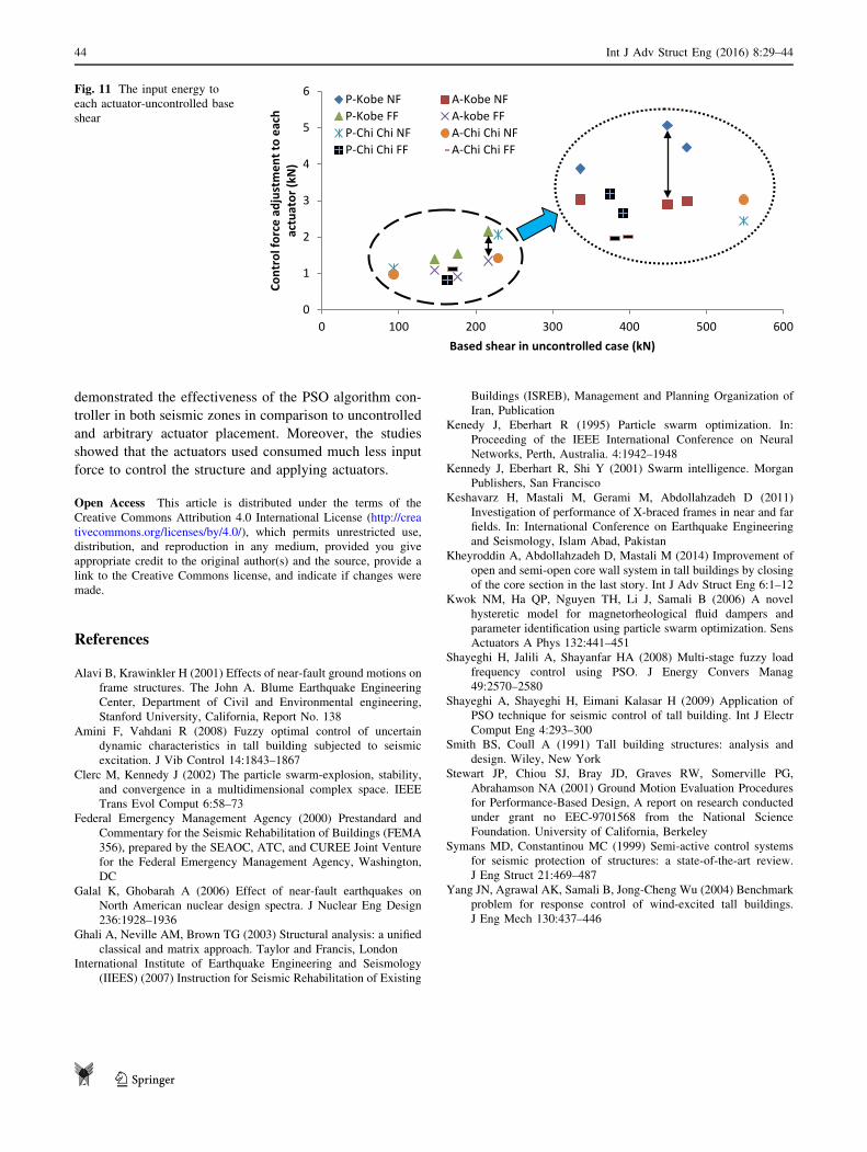
buildings is determined.

According to Fig. 11, the base shear value was a func-

tion of the external excitation and the structure properties,

which increased the base shear accompanied by the actu-

ator force increase. Input actuator force was computed

based on Eq. (16). Moreover, by increasing the shear force

at the base level of the structure, the difference between

actuator force obtained from the optimized and arbitrary

cases was increased. Concerning the results obtained in

Fig. 11, the required force for actuators varied in the range

of 0.4–1.2 % of the total base shear.

Conclusion

In this study, by using active actuators in the braces, three

different building heights were controlled under external

excitations where concrete shear walls were used as sec-

ondary lateral load-resisting system in the buildings. The

placement of actuators was implemented by using opti-

mization employing the PSO algorithm method and arbi-

trarily for both near- and far-field earthquake zones.

Concerning the results obtained, the performance of the

controller using the PSO algorithm method was signifi-

cantly better than the arbitrary placement of actuators in all

seismic zones. By considering the effects of seismic zone,

most actuators were placed on the upper third of the

structure in tall buildings, while for the moderate and short

buildings, most actuators were placed on the upper half of

the structure. The defined performance criteria

Near field of Kobe Earthquake Far field of Kobe earthquake


-0.8

-0.6

-0.4

-0.2

0

0.2

0.4

0.6

0.4 0.6 0.8 1

Effe

cien

cy o

f alg

orith

m c

ontro

l in

perf

orm

ance

crit

eria

Height ratio

J1 J2 J3 J4

J5 J6 J7

-0.6

-0.4

-0.2

0

0.2

0.4

0.6

0.4 0.6 0.8 1

Effe

cien

cy o

f alg

orith

m c

ontro

l in

perf

orm

ance

crit

eria

Height ratio

J1 J2 J3 J4

J5 J6 J7

-0.4

-0.3

-0.2

-0.1

0

0.1

0.2

0.3

0.4

0.4 0.6 0.8 1

Effe

cien

cy o

f con

trol a

lgor

ithm

on

perf

orm

ance

crit

eria

Height ratio

J1 J2 J3 J4J5 J6 J7

-0.4

-0.3

-0.2

-0.1

0

0.1

0.2

0.3

0.4

0.4 0.5 0.6 0.7 0.8 0.9 1Ef

feci

ency

of c

ontro

l alg

orith

m o

n pe

rfor

man

ce c

riter

ia

Height ratio

J1 J2 J3 J4

J5 J6 J7

Fig. 10 Efficiency variations of defined performance criteria throughout the height ratio


123

demonstrated the effectiveness of the PSO algorithm con-

troller in both seismic zones in comparison to uncontrolled

and arbitrary actuator placement. Moreover, the studies

showed that the actuators used consumed much less input

force to control the structure and applying actuators.

Open Access This article is distributed under the terms of the

Creative Commons Attribution 4.0 International License (http://crea

tivecommons.org/licenses/by/4.0/), which permits unrestricted use,

distribution, and reproduction in any medium, provided you give

appropriate credit to the original author(s) and the source, provide a

link to the Creative Commons license, and indicate if changes were

made.

References

Alavi B, Krawinkler H (2001) Effects of near-fault ground motions on

frame structures. The John A. Blume Earthquake Engineering

Center, Department of Civil and Environmental engineering,

Stanford University, California, Report No. 138

Amini F, Vahdani R (2008) Fuzzy optimal control of uncertain

dynamic characteristics in tall building subjected to seismic

excitation. J Vib Control 14:1843–1867

Clerc M, Kennedy J (2002) The particle swarm-explosion, stability,

and convergence in a multidimensional complex space. IEEE

Trans Evol Comput 6:58–73

Federal Emergency Management Agency (2000) Prestandard and

Commentary for the Seismic Rehabilitation of Buildings (FEMA

356), prepared by the SEAOC, ATC, and CUREE Joint Venture

for the Federal Emergency Management Agency, Washington,

DC

Galal K, Ghobarah A (2006) Effect of near-fault earthquakes on

North American nuclear design spectra. J Nuclear Eng Design

236:1928–1936

Ghali A, Neville AM, Brown TG (2003) Structural analysis: a unified

classical and matrix approach. Taylor and Francis, London

International Institute of Earthquake Engineering and Seismology

(IIEES) (2007) Instruction for Seismic Rehabilitation of Existing

Buildings (ISREB), Management and Planning Organization of

Iran, Publication

Kenedy J, Eberhart R (1995) Particle swarm optimization. In:

Proceeding of the IEEE International Conference on Neural

Networks, Perth, Australia. 4:1942–1948

Kennedy J, Eberhart R, Shi Y (2001) Swarm intelligence. Morgan

Publishers, San Francisco

Keshavarz H, Mastali M, Gerami M, Abdollahzadeh D (2011)

Investigation of performance of X-braced frames in near and far

fields. In: International Conference on Earthquake Engineering

and Seismology, Islam Abad, Pakistan

Kheyroddin A, Abdollahzadeh D, Mastali M (2014) Improvement of

open and semi-open core wall system in tall buildings by closing

of the core section in the last story. Int J Adv Struct Eng 6:1–12

Kwok NM, Ha QP, Nguyen TH, Li J, Samali B (2006) A novel

hysteretic model for magnetorheological fluid dampers and

parameter identification using particle swarm optimization. Sens

Actuators A Phys 132:441–451

Shayeghi H, Jalili A, Shayanfar HA (2008) Multi-stage fuzzy load

frequency control using PSO. J Energy Convers Manag

49:2570–2580

Shayeghi A, Shayeghi H, Eimani Kalasar H (2009) Application of

PSO technique for seismic control of tall building. Int J Electr

Comput Eng 4:293–300

Smith BS, Coull A (1991) Tall building structures: analysis and

design. Wiley, New York

Stewart JP, Chiou SJ, Bray JD, Graves RW, Somerville PG,

Abrahamson NA (2001) Ground Motion Evaluation Procedures

for Performance-Based Design, A report on research conducted

under grant no EEC-9701568 from the National Science

Foundation. University of California, Berkeley

Symans MD, Constantinou MC (1999) Semi-active control systems

for seismic protection of structures: a state-of-the-art review.

J Eng Struct 21:469–487

Yang JN, Agrawal AK, Samali B, Jong-Cheng Wu (2004) Benchmark

problem for response control of wind-excited tall buildings.

J Eng Mech 130:437–446

0

1

2

3

4

5

6

0 100 200 300 400 500 600

Cont

rol f

orce

adj

ustm

ent t

o ea

ch

actu

ator

(kN

)

Based shear in uncontrolled case (kN)

P-Kobe NF A-Kobe NFP-Kobe FF A-kobe FFP-Chi Chi NF A-Chi Chi NFP-Chi Chi FF A-Chi Chi FF

Fig. 11 The input energy to

each actuator-uncontrolled base

shear


123

http://creativecommons.org/licenses/by/4.0/

http://creativecommons.org/licenses/by/4.0/

Documents

Optimal placement of active braces by using PSO · PDF fileOptimal placement of active braces by using PSO algorithm ... concrete shear walls and core wall systems. ... The applied