Mitchel Craun1

Mechanical Engineering,University of California, Santa Barbara,

Santa Barbara, CA 93106e-mail: craun@umail.ucsb.edu

Bassam BamiehMechanical Engineering,

University of California, Santa Barbara,Santa Barbara, CA 93106

Optimal Periodic Control of anIdeal Stirling Engine ModelWe consider an optimal control problem for a model of a Stirling engine that is activelycontrolled through its displacer piston motion. The framework of optimal periodic control(OPC) is used as the setting for this active control problem. We use the idealized isother-mal Schmidt model for the system dynamics and formulate the control problem so as tomaximize mechanical power output while trading off a penalty on control (displacermotion) effort. An iterative first-order algorithm is used to obtain the optimal periodicmotion of the engine and control input. We show that optimal motion is typically nonsinu-soidal with significant higher harmonic content, and that a significant increase in thepower output of the engine is possible through the optimal scheduling of the displacermotion. These results indicate that OPC may provide a framework for a large class ofenergy conversion and harvesting problems in which active actuation is available.[DOI: 10.1115/1.4029682]

1 Introduction

Stirling engines are heat air engines that can operate using anyheat power source such as external combustion, waste heat, orsolar thermal power. They are receiving renewed interest as apotentially competitive energy conversion technology in severaldomains including micro combined heat and power (such as theWhisperGen units made by WisperTech, Christchurch, New Zea-land), and solar thermal energy conversion (such as those madeby SunPower, Inc., Athens, OH and Infinia Corp., Ogden, UT).

There has been recent interest in more detailed modeling andoptimization of Stirling engines and coolers [1]. Related recentwork on control-oriented modeling of a Stirling engine was donein Refs. [2–5], while the concept of an Active Stirling Engine [6]has been recently proposed. This latter concept is similar to ourcurrent work, where the displacer piston motion is the controlinput. Rather than let displacer motion be determined by themechanical engine design (whether in kinematically linkedengines or the free-piston variety), this new Stirling engine con-cept is based on directly actuating the displacer piston. This pro-vides a large amount of control authority over the enginedynamics. A natural question then is how to exploit this new con-trol possibility to optimize the operation of the engine, andwhether significant increases in efficiency and/or power outputcan be achieved. In contrast to Ref. [6], where the control objec-tive is for the displacer to track a predetermined trajectory, we for-mulate a problem where the periodic piston motions and thethermodynamic cycle itself are optimally designed.

In this paper, we cast the active control problem of a Stirlingengine as a problem in OPC. This is motivated by the observationthat the ultimate motion of such devices is cyclical, but the opti-mal limit cycle is not known a priori, but is to be designed throughthe optimal control problem. We therefore do not have a tradi-tional trajectory tracking problem, but rather a problem of optimaltrajectory design with periodic boundary conditions, i.e., optimallimit cycle design. Since one of the main concerns with Stirlingengines is their relatively low power density, we setup a problemwhere the mechanical power output is to be maximized whiletrading off the control effort.

This paper is organized as follows: Section 2 describes thedynamical model used, which is the so-called isothermal Schmidt

model. This is the simplest possible model of a Stirling engine andis used as a proof-of-concept to illustrate the advantages of optimalcycle design. The methodology presented is, however, applicableto higher fidelity engine models as well. Section 3 sets up optimalcycle design as an OPC problem and presents the iterative numeri-cal hill climbing algorithm we used. There are special issuesintroduced by the periodic boundary conditions which requirecareful treatment, and these are discussed in some detail. Finally,Section 4 presents a case study with numerical results, togetherwith a comparison to a well-designed kinematically linked,beta-type Stirling engine. Significant output mechanical powerimprovement on the order of 40% was achieved for this example.

2 Dynamic Modeling

A Stirling engine is an air engine in which pressure oscillationsdrive a power piston that performs mechanical work on a load.These pressure oscillations are in turn driven by the mechanicalmotion of both power and displacer pistons. We present the sim-plest possible model for this engine, the so-called isothermalSchmidt model. The first model in Sec. 2.1 is that of an enginewith an actuated displacer but without kinematic linkages betweenpower and displacer pistons (Fig. 1(c)). We use this model foroptimal cycle design. The second model in Sec. 2.2 has flywheelkinematic linkages, resulting in a so-called beta-type engine(Fig. 1(b)), which we use as a benchmark case for performancecomparisons.

2.1 The Basic Isothermal Model. Figure 1(a) is a diagramof the basic compartments and pistons of a Stirling engine. Theengine is composed of three sections, the hot and cold chambersand the regenerator. The hot chamber is in thermal contact with aheat source, and the cold chamber is in thermal contact with aheat sink. Gas can move between the two chambers through theregenerator channel. The power piston performs work on a load,while the displacer piston’s primary task is to move the workinggas between the hot and cold chambers through the regenerator.Mechanical motion induces thermodynamic changes as follows:as the displacer piston oscillates, air is shuttled between the hotand cold chambers through the regenerator channel. This shuttlingcreates oscillations in the average (over all sections) gas tempera-ture, which in turn cause oscillations in engine pressure. The pres-sure oscillations drive the power piston, which is how the gasthermodynamics induce mechanical motion. In a beta-type enginesuch as the one shown in Fig. 1(b), the kinematic linkages providea feedback path between the power piston motion and displacer

1Corresponding author.Contributed by the Dynamic Systems Division of ASME for publication in the

JOURNAL OF DYNAMIC SYSTEMS, MEASUREMENT, AND CONTROL. Manuscript receivedAugust 28, 2013; final manuscript received December 22, 2014; published onlineMarch 4, 2015. Assoc. Editor: John B. Ferris.

Journal of Dynamic Systems, Measurement, and Control JULY 2015, Vol. 137 / 071002-1Copyright VC 2015 by ASME

Downloaded From: http://dynamicsystems.asmedigitalcollection.asme.org/ on 03/05/2015 Terms of Use: http://asme.org/terms

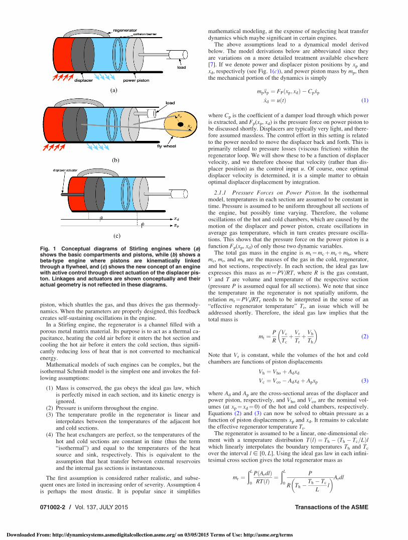
piston, which shuttles the gas, and thus drives the gas thermody-namics. When the parameters are properly designed, this feedbackcreates self-sustaining oscillations in the engine.

In a Stirling engine, the regenerator is a channel filled with aporous metal matrix material. Its purpose is to act as a thermal ca-pacitance, heating the cold air before it enters the hot section andcooling the hot air before it enters the cold section, thus signifi-cantly reducing loss of heat that is not converted to mechanicalenergy.

Mathematical models of such engines can be complex, but theisothermal Schmidt model is the simplest one and invokes the fol-lowing assumptions:

(1) Mass is conserved, the gas obeys the ideal gas law, whichis perfectly mixed in each section, and its kinetic energy isignored.

(2) Pressure is uniform throughout the engine.(3) The temperature profile in the regenerator is linear and

interpolates between the temperatures of the adjacent hotand cold sections.

(4) The heat exchangers are perfect, so the temperatures of thehot and cold sections are constant in time (thus the term“isothermal”) and equal to the temperatures of the heatsource and sink, respectively. This is equivalent to theassumption that heat transfer between external reservoirsand the internal gas sections is instantaneous.

The first assumption is considered rather realistic, and subse-quent ones are listed in increasing order of severity. Assumption 4is perhaps the most drastic. It is popular since it simplifies

mathematical modeling, at the expense of neglecting heat transferdynamics which maybe significant in certain engines.

The above assumptions lead to a dynamical model derivedbelow. The model derivations below are abbreviated since theyare variations on a more detailed treatment available elsewhere[7]. If we denote power and displacer piston positions by xp andxd, respectively (see Fig. 1(c)), and power piston mass by mp, thenthe mechanical portion of the dynamics is simply

mp€xp ¼ FPðxp; xdÞ $ Cp _xp

_xd ¼ uðtÞ (1)

where Cp is the coefficient of a damper load through which poweris extracted, and Fp(xp, xd) is the pressure force on power piston tobe discussed shortly. Displacers are typically very light, and there-fore assumed massless. The control effort in this setting is relatedto the power needed to move the displacer back and forth. This isprimarily related to pressure losses (viscous friction) within theregenerator loop. We will show these to be a function of displacervelocity, and we therefore choose that velocity (rather than dis-placer position) as the control input u. Of course, once optimaldisplacer velocity is determined, it is a simple matter to obtainoptimal displacer displacement by integration.

2.1.1 Pressure Forces on Power Piston. In the isothermalmodel, temperatures in each section are assumed to be constant intime. Pressure is assumed to be uniform throughout all sections ofthe engine, but possibly time varying. Therefore, the volumeoscillations of the hot and cold chambers, which are caused by themotion of the displacer and power piston, create oscillations inaverage gas temperature, which in turn creates pressure oscilla-tions. This shows that the pressure force on the power piston is afunction Fp(xp, xd) of only those two dynamic variables.

The total gas mass in the engine is mt¼mcþmrþmh, wheremc, mr, and mh are the masses of the gas in the cold, regenerator,and hot sections, respectively. In each section, the ideal gas lawexpresses this mass as m¼PV/RT, where R is the gas constant,V and T are volume and temperature of the respective section(pressure P is assumed equal for all sections). We note that sincethe temperature in the regenerator is not spatially uniform, therelation mr¼PVr/RTr needs to be interpreted in the sense of an“effective regenerator temperature” Tr, an issue which will beaddressed shortly. Therefore, the ideal gas law implies that thetotal mass is

mt ¼P

R

Vc

Tcþ Vr

Trþ Vh

Th

! "(2)

Note that Vr is constant, while the volumes of the hot and coldchambers are functions of piston displacements

Vh ¼ Vho þ Adxd

Vc ¼ Vco $ Adxd þ Apxp (3)

where Ad and Ap are the cross-sectional areas of the displacer andpower piston, respectively, and Vho and Vco are the nominal vol-umes (at xp¼ xd¼ 0) of the hot and cold chambers, respectively.Equations (2) and (3) can now be solved to obtain pressure as afunction of piston displacements xp and xd. It remains to calculatethe effective regenerator temperature Tr.

The regenerator is assumed to be a linear, one-dimensional ele-ment with a temperature distribution TðlÞ ¼ Th $ Th $ Tc=Lð Þlwhich linearly interpolates the boundary temperatures Th and Tc

over the interval l ! [0, L]. Using the ideal gas law in each infini-tesimal cross section gives the total regenerator mass as

mr ¼ðL

0

PðArdlÞRTðlÞ

¼ðL

0

P

R Th $Th $ Tc

Ll

! "Ardl

Fig. 1 Conceptual diagrams of Stirling engines where (a)shows the basic compartments and pistons, while (b) shows abeta-type engine where pistons are kinematically linkedthrough a flywheel, and (c) shows the new concept of an enginewith active control through direct actuation of the displacer pis-ton. Linkages and actuators are shown conceptually and theiractual geometry is not reflected in these diagrams.

071002-2 / Vol. 137, JULY 2015 Transactions of the ASME

Downloaded From: http://dynamicsystems.asmedigitalcollection.asme.org/ on 03/05/2015 Terms of Use: http://asme.org/terms

where Ar is the cross-sectional area through which fluid can flowin the regenerator. This integral yields

mr ¼PVr

RðTh $ TcÞln

Th

Tc

! "(4)

where Vr is the volume of the regenerator. We now observe thatEq. (4) is an ideal gas law for the regenerator if its temperature istaken as

Tr : ¼ Th $ Tc

lnTh

Tc

! " (5)

Solving Eq. (2) for pressure and substituting for the variablesVh, Vc, and Tr from Eqs. (3) and (5) gives

P ¼ mtR

Vc

Tcþ Vr

Trþ Vh

Th

! "

P ¼ mtR

Vco

Tcþ Vho

Thþ

VrlnTh

Tc

! "

Th $ Tc$ Ad

Tcxd þ

Ap

Tcxp þ

Ad

Thxd

0

BB@

1

CCA

(6)

For notational clarity, the following constants are defined:

ap : ¼Ap

TcVmt; ad :¼ Ad

Vmt

1

Tc$ 1

Th

$ %

Vmt : ¼Vho

Thþ

VrlnTh

Tc

! "

Th $ Tcþ Vco

Tc

and the expression (6) can be more clearly rewritten as a functionof piston displacements

P ¼ mtR

Vmt

1

1þ apxp $ adxd

! "(7)

The above expression for the pressure finally gives the pressureforce term Fp(xp, xd) in Eq. (1), and the engine dynamics can nowbe rewritten as

mp€xp ¼ ApPm1

1þ apxp $ adxd$ 1

$ %$ Cp _xp

_xd ¼ uðtÞ (8)

where Pm:¼mtR/Vmt is the nominal pressure (at xp¼ xd¼ 0),which is also assumed to be equal to the pressure on the externalside of the power piston.1

2.1.2 Pressure Losses in Regenerator and Control Power.Although in the derivation, pressure was assumed uniform

throughout the engine, there is in reality a small pressure drop dueto viscous friction when fluid flows across the regenerator matrixmaterial. In an actively controlled Stirling engine (Fig. 1(c)), theactuator primarily works against that small pressure drop, whichwe need to characterize in order to quantify control effort. Wepoint out that this pressure drop is typically much smaller than thepressure oscillations in the engine, which is the reason it can beneglected when calculating the force on the power piston in the

previous section. This fact is recognized in traditional Stirlingengines. It is also true in our controlled engine with optimallydesigned cycle as a consequence of the optimization objective(18). Maximization of this objective has the consequence of insur-ing that viscous losses (which are related to control power) arekept at a minimum compared with pressure oscillations (whichdetermine the output power of the engine).

A standard model [7] for viscous pressure loses assumes themto be in the same direction as the average flow velocity vr, butproportional in magnitude to its square

DP ¼ qrfL

rhvrð Þ26 (9)

where we have used the following notation for the “signed square”function að Þ26:¼ ajaj. The constants in the above expression arethe fluid density qr, f is the Fanning friction factor, L the length ofthe regenerator, and rh is the hydraulic radius.

By conservation of mass, the average flow velocity vr can berelated to the cold and hot sections’ mass flow rates by

qrvrAr ¼1

2_mc $ _mhð Þ ¼ 1

2

d

dtqcVc $ qhVhð Þ (10)

where qc and qh are the fluid densities in the cold and hot sections,respectively. Using the ideal gas law with the assumption thatpressure is uniform throughout, the densities can be expressed as

qr ¼P

RTr; qh ¼

P

RTh; qc ¼

P

RTc(11)

The relative amplitudes of density oscillations are typically verysmall and therefore taken as constant. This simplifies the timederivative in Eq. (10) and yields the following expression forregenerator flow velocity as a function of the pistons’ velocities:

vr ¼Tr

2Ar

Ap

Tc_xp $

AdðTc þ ThÞTcTh

_xd

! "(12)

This last expression for vr and the expression (9) for the pres-sure loss now give an expression for the control power required interms of the state variables and input. If the displacer piston isassumed to be nearly massless, then the force Fd needed to drivethe displacer is equal and opposite to the force due to pressure dif-ference across the displacer, which is just the pressure loss in theregenerator. The instantaneous control power is therefore theproduct of that force with displacer velocity yielding

Instantaneous control power ¼ Fd _xd ¼ $AdDPð Þ _xd

¼ AdqrfLT2r

4rhA2r

AdðTc þ ThÞTcTh

_xd $Ap

Tc_xp

! "2

6

_xd (13)

2.2 Model of a Beta-Type Engine. This traditional type ofStirling engine has kinematic linkages and no active control. Weuse it as a benchmark design for performance comparison withour engine with optimally designed cycle. A typical beta Stirlingengine design is shown in Fig. 1(b). Any parameters in commonbetween the beta engine and the actively controlled one (Fig. 1(c))were set equal. The main difference between the two is that kine-matic linkages enforce constraints between the power and dis-placer piston motions. The dynamics for the beta engine can bewritten down using the model (8) and the geometrical relationsfrom Fig. 1(b) as follows:

mp€xp ¼ ApPm1

1þ apxp $ adxd$ 1

$ %$ Cp _xp $ Fp (14)

I €h ¼ FpRpsinðh$ /Þ $ AdRdDPsinðhÞ (15)

1In other words, the origins of the xp and xd axes are chosen such that atxp¼ xd¼ 0, internal engine pressure is equal to the external atmospheric pressure.This makes the zero state an equilibrium of the dynamics.

Journal of Dynamic Systems, Measurement, and Control JULY 2015, Vol. 137 / 071002-3

Downloaded From: http://dynamicsystems.asmedigitalcollection.asme.org/ on 03/05/2015 Terms of Use: http://asme.org/terms

xd ¼ $Rd cosðhÞ (16)

xp ¼ $Rp cosðh$ /Þ (17)

where I and h are the moment of inertia and angular position ofthe flywheel, respectively, Fp is the reaction force between thepower piston and the flywheel, / is the phase difference betweenthe two pistons, Rp and Rd are the radial attachment locations ofthe pistons on the flywheel, and DP is the pressure differenceacross the displacer caused by forcing the working fluid to flowthrough the regenerator (Eq. (9)). These equations were derivedassuming that the displacer and the arms connecting the pistons tothe flywheel are massless. The latter are assumed to be sufficientlylong so that the forces they exert on the flywheel and pistons areessentially horizontal.

3 Optimal Cycle Design

The goal is to find the cyclical displacer motion which willmaximize the average net power produced by the Stirling engineover one period. We formulate this problem as an OPC problem,which is a standard optimal control problem, but with periodicboundary conditions. We then outline a first-order numericalmethod referred to as “hill climbing” to maximize the objective.The issue of enforcing periodic boundary conditions on both thestate and co-state equations requires some special care which isexpounded on in Sec. 3.3.

OPC has been an area of active research in the past, and itwould be difficult to give a complete background here. Some ofthe more notable work [8–12] was partially motivated by energyefficiency problems starting in the 1970s. That work was domi-nated by the question of when cycling is more efficient thansteady operation. However, here we have a slightly different set-ting in that the engines we deal with naturally (i.e., without con-trol) would cycle. The availability of a control input then givesthe additional design freedom of finding non-natural limit cyclesthat are energetically more favorable. The basic theoretical frame-work of OPC is, however, common to our present work and theearlier literature.

3.1 Optimal Control Problem Formulation. Power isextracted from the engine via a damper attached to the power pis-ton, and some power is used up by the displacer actuator to workagainst viscous pressure losses across the regenerator. The aver-age net power over one cycle is the difference between the twoand is given by

J ¼ 1

T

ðT

0

/ðx; uÞdt ¼ 1

T

ðT

0

Cp _x2p $ Fdu

& 'dt (18)

The dynamics are given by Eq. (8) and the control power Fdu is

Fdu ¼ a adu$ ap _xp

( )2

6u (19)

where the constants a, ad, and ap are given by Eq. (13). The periodT is fixed in this formulation, and a search of a set of periods isdone as an outer loop in the algorithm. All states and the controlare required to satisfy periodic boundary conditions

xpð0Þ ¼ xpðTÞ; _xpð0Þ ¼ _xpðTÞ; xdð0Þ ¼ xdðTÞ;uð0Þ ¼ uðTÞ (20)

A final constraint we require is that of no collision between thepistons and the collision barrier or the engine walls. These can beexpressed using the inequality constraints

Ld & xdðtÞ& "Ld

Lp & xpðtÞ(21)

where Ld; Lp, and "Ld are the lower and upper limits on the dis-placer and power pistons’ positions, respectively. Hard limit con-straints such as these are typically difficult to enforce in numericaloptimal control problems, so a “soft constraints” approach is usedby augmenting the objective with suitably designed penalty func-tions Pd and Pp that grow unboundedly as the states approach theconstraints

J ¼ 1

T

ðT

0

Cp _x2p $ Fdu$ PdðxdÞ $ PpðxpÞ

& 'dt (22)

In summary, our optimal control problem has the dynamics

_x1 ¼ x2

_x2 ¼ApPm

mp

1

1þ apx1 $ adx3$ 1

$ %$ Cp

mpx2

_x3 ¼ u

(23)

where x1:¼ xp, x2 :¼ _xp, and x3:¼ xd. The boundary conditions(20) are T-periodic. The objective is to maximize the performance

J ¼ 1

T

ðT

0

Cpx22 $ a adu$ apx2

( )2

6u$ Pdðx3Þ $ Ppðx1Þ& '

dt (24)

3.1.1 First-Order Variations. In deriving first-order necessaryconditions for optimality as well as first-order numerical algo-rithms, it is useful to calculate variations using a costate as aLagrange multiplier. These calculations are standard in any opti-mal control textbook [13–15], so we only recap what we needhere to highlight the role of periodic boundary conditions. Con-sider an optimal control problem with the dynamical constraint

_x ¼ f ðx; uÞ; xð0Þ ¼ xðTÞ (25)

and the performance objective J ¼ 1=Tð ÞÐ T

0 /ðx; uÞdt: A Lagran-gian objective J is defined using a Lagrange multiplier functionk(t), t ! [0, T] termed the costate by

J :¼ 1

T

ðT

0

/ðx; uÞ $ kT _x$ f ðx; uÞð Þ( )

dt (26)

The standard calculus of variations argument including an integra-tion by parts yields the following expression for the variationsin J :

dJ ¼ 1

T

ðT

0

@/@xþ _kT þ kT @f

@x

$ %dx dt$ ½kTðTÞ $ kTð0Þ(dxð0Þ

!

þðT

0

@/@uþ kT @f

@u

$ %du dt

"ð27Þ

where the state equation _x ¼ f ðx; uÞ and its periodic boundaryconditions x(0)¼ x(T)) dx(0)¼ dx(T) have been used. If in addi-tion, the costate is forced to satisfy the following adjoint equationwith periodic boundary conditions:

_k ¼ $ @f

@x

! "T

k$ @/@x

! "T

; kð0Þ ¼ kðTÞ (28)

then variations in J can finally be expressed as

dJ ¼ 1

T

ðT

0

@/@uðx; uÞ þ kT @f

@uðx; uÞ

$ %du dt (29)

where u, x, and k satisfy Eqs. (25) and (28). When deriving first-order necessary conditions for optimality, the term in square

071002-4 / Vol. 137, JULY 2015 Transactions of the ASME

Downloaded From: http://dynamicsystems.asmedigitalcollection.asme.org/ on 03/05/2015 Terms of Use: http://asme.org/terms

brackets in Eq. (29) is set to zero. Alternatively, this expressionfor dJ is used to propose updates to control inputs in an iterativenumerical algorithm, which is presented in the next section.

3.2 Hill Climbing. Expression (29) can be used to build aniterative algorithm for maximizing the objective (thus the term“hill climbing”). The initialization step consists of applying someperiodic input u0 to the system and obtaining the correspondingperiodic state trajectory x0. For each subsequent step, let (un, xn)be the functions obtained at the nth step of the algorithm, then thenext iteration is chosen according to

_kn ¼ $@f

@xðxn; unÞ

! "T

kn $@/@xðxn; unÞ

! "T

knðTÞ ¼ knð0Þ (30)

unþ1 ¼ un þ e@/@uðxn; unÞ þ kT

n

@f

@uðxn; unÞ

! "(31)

_xnþ1 ¼ f ðxnþ1; unþ1Þ; xnþ1ðTÞ ¼ xnþ1ð0Þ (32)

Several remarks can be made about this algorithm

• Since (un, xn, kn) simultaneously satisfy the sate and costateequations, the expression (29) for the variation guaranteesthat if (du)n:¼ unþ 1$ un is chosen according to Eq. (31),then

dJ ¼ 1

T

ðT

0

@/@uðx; uÞ þ kT @f

@uðx; uÞ

$ %2

dt ) 0

and thus there exists a sufficiently small step size e such thatthe value of the objective at step nþ 1 is improved over thatat step n.

• Both Eqs. (32) and (30) require finding T-periodic solutionsto the corresponding differential equations. These issues arecarefully addressed in Sec. 3.3.

The method just described is a standard one in numerical opti-mal control and was first used for periodic optimal control prob-lems by Horn and Lin [16]. Similar methods have also been usedby Kowler and Kadlec [17] and van Noorden et al. [18]. There aretwo main distinctions between their algorithms and ours. The firstis that the existence of periodic solutions to the costate equation(28) was implicitly assumed and not addressed in Refs. [16–18].These equations do not always admit periodic solutions, and weanalyze conditions that guarantee existence in the sequel. The sec-ond distinction is in how the periodic state and costate trajectoriesare determined. A Newton–Raphson iteration is used in Refs. [16]and [17] to find the periodic state trajectories, and then the costatetrajectories are found by a decomposition into homogeneous andparticular solutions. A more sophisticated Newton–Picard itera-tive algorithm is used in Ref. [18] to solve for both the state andcostate trajectories. In the present work, the state trajectories werefound by simply simulating the state equations for sufficientlylong times to reach periodic steady-state conditions. For problemswith slow dynamics, it is preferable to use an iterative method tofind the periodic state trajectories associated with a given input.However, the dynamics associated with our problem convergedrelatively quickly, so the added complexity associated with aniterative routine was not deemed necessary. To find the periodiccostate trajectories, we developed an algorithm described inSec. 3.3, which uses the variation of constants formula to find theperiodic boundary conditions directly.

3.3 Enforcing Periodicity. We begin with enforcing the peri-odicity of the state equation (32) as it is the simpler case. Sincethe input enters the dynamics through an integrator (the equationfor _x3 in Eq. (23)), a necessary condition for x3 to be periodic is

for u to have zero average in time. Therefore, the zero-averageconstraint on controls needs to be added to our OPC problem. It isnot difficult to show2 that this amounts to simply removing anyDC component of unþ 1 in Eq. (31) at every step of the iteration.While this is a necessary but not sufficient condition for theperiodicity of the state trajectory, it was found through extensivenumerical experiments that this condition alone resulted in a T-periodic steady-state trajectory (after simulation over severalcycles) of Eq. (32) when the input is T-periodic and has zeromean. This is likely due to the physical nature of this particularmodel.

As for the costate equation (28), note that it is a linear, periodi-cally time-varying system (for k) where the function @/=@xð ÞT isan input. It is thus of the form

_kðtÞ ¼ AðtÞkðtÞ þ BðtÞ; kð0Þ ¼ kðTÞ (33)

where both A(.) and B(.) are periodic functions with period T. Theperiodic boundary condition k(0)¼ k(T) amounts to requiring thisequation to have a T-periodic solution. However, it is not alwaystrue that a linear T-periodically time-varying system with a T-periodic input must have a T-periodic trajectory, more complexbehavior can occur [19]. Here, we give conditions for the requiredperiodic solution to exist, and then show how the additional flexi-bility available through selecting penalty functions can be used toinsure this condition is satisfied.

First, we show how all initial conditions leading to T-periodicsolutions can be characterized. Using the variations-of-constantsformula on (33) gives

kðTÞ ¼ UðT; 0Þkð0Þ þðT

0

UðT; tÞBðtÞdt (34)

where U is the state transition matrix of the system. Now the exis-tence of an initial condition leading to a periodic solution"k ¼ kð0Þ ¼ kðTÞ is equivalent to the existence of a vector "k thatsolves the following matrix–vector equation:

I $ UðT; 0Þð Þ"k ¼ðT

0

UðT; tÞBðtÞdt (35)

We note that if such initial conditions exist, their calculation is alinear algebra problem. The vector

Ð T0 UðT; tÞBðtÞdt is calculated

from a simulation of a linear system with zero initial conditions,while the matrix U(T, 0) can be calculated in the standard mannerfrom a number of linear initial value problems. After these calcu-lations, the linear system of equations (35) can be solved for "k.

It now remains to provide conditions as to when the system(35) has solutions "k, or equivalently as to when the linear, T-periodic system (33) has T-periodic solutions. This question haspreviously been addressed in the literature [19]. We rephrase themain result here in a form that is directly applicable to the presentproblem.

THEOREM 1. The following three statements are equivalent:

• The linear T-periodic system

_kðtÞ ¼ AðtÞkðtÞ þ BðtÞ (36)

has a T-periodic solution, i.e., such that k(0)¼ k(T).• The following matrix–vector equation has a solution "k:

I $ UðT; 0Þð Þ"k ¼ðT

0

UðT; tÞBðtÞdt (37)

2This follows from the observation that unþ 1$ nn needs to be in the direction duthat maximizes (29) subject to the constraint of zero average. This direction issimply the projection of the square bracketed term onto the subspace of zero-averagesignals, i.e., removing the DC term.

Journal of Dynamic Systems, Measurement, and Control JULY 2015, Vol. 137 / 071002-5

Downloaded From: http://dynamicsystems.asmedigitalcollection.asme.org/ on 03/05/2015 Terms of Use: http://asme.org/terms

where U is the state transition matrix of A.• For any T-periodic solution z of the homogenous adjoint sys-

tem _zðtÞ ¼ $A*ðtÞzðtÞ; the following orthogonality conditionholds: ðT

0

zTðtÞBðtÞdt ¼ 0 (38)

Furthermore, each T-periodic solution of Eq. (36) is such thatkð0Þ ¼ "k, where "k is a solution to Eq. (37), and vice versa, i.e.,there is a one-to-one correspondence between T-periodic solu-tions of Eq. (36) and vector solutions of Eq. (37).

This theorem is a reformulation of a result in Ref. [19], Sec.2.10, Lemma I. For completeness, we provide a brief, self-contained proof in the Appendix. Condition (38) can be used tocheck whether a given system has T-periodic solutions, then solu-tions of the matrix–vector equation (37) are used to find the corre-sponding initial conditions, and thus the T-periodic solutions.

To see the consequences of condition (38) to the present prob-lem, Eq. (30) is written out explicitly after reference to the dynam-ics (23) and performance objective (24)

_k1

_k2

_k3

2

664

3

775 ¼

0apðApPm=mpÞ

ð1þ apx1 $ adx3Þ20

$1Cp

mp0

0$adðApPm=mpÞð1þ apx1 $ adx3Þ2

0

2

666666664

3

777777775

k1

k2

k3

2

64

3

75$

P0pðx1Þ

@/@x2

P0dðx3Þ

2

6664

3

7775

(39)

where P0 stands for the derivative of the corresponding single-variable function P, and the exact form of @/=@x2 is irrelevant inthe sequel. To apply Theorem 1, we note that A :¼ $ @f=@xð ÞTabove has the following left null vector:

vn ¼ ad 0 ap½ (

for any state trajectory. This implies that zn :¼ vTn is always a right

null vector for the adjoint system _z ¼ $ATðtÞz, and thus gives con-stant (and therefore T-periodic) solutions. Condition (38) appliedto this solution zTðtÞ ¼ ad 0 ap½ ( gives the requirement

ðT

0

adP0p x1ðtÞð Þ þ apP0d x3ðtÞð Þ& '

dt ¼ 0 (40)

Extensive numerical investigations were carried out, and no otherperiodic solutions of the homogenous system adjoint to Eq. (39)were found. We thus proceed with the assumption that condition(40) is the only one that needs to be checked.

In our routines, the constraint (40) is enforced on each term inthe integral separately. Consider the displacer position penaltyfirst. A sketch of a typical Pd is shown in Fig. 2, where it is termedthe “fixed penalty.” This penalty has even symmetry about themidpoint of ½Ld; "Ld(, and therefore P0d has corresponding odd sym-metry.3 If the trajectory of xd is symmetric in time about the mid-point, then clearly the integral of P0dðxdðtÞÞ over one periodic willbe zero. However, as is typical in the initial steps of the algorithm,xd may not have that temporal symmetry. We therefore augmentPd with an additional function (termed “variable penalty” inFig. 2), which has variable parameters Sd and "Sd. These parame-ters essentially bias the even symmetry of the augmented Pd (andconsequently the odd symmetry of P0d). Therefore even when thetrajectory xd does not have temporal symmetry about the mid-point, parameters Sd and "Sd can be found such that the integral ofthe augmented P0dðxdðtÞÞ is zero over one period. This augmentedpenalty function retains the barrier penalty features at Ld and "Ld

of the original one and has the additional property of satisfyingthe integral constraint. A similar technique is used for the powerpiston penalty function as illustrated in the bottom part of Fig. 2.Those details are omitted for brevity. Finally, we note that at eachstep of the iteration, the parameters Sd; "Sd, and Sp required toenforce Eq. (40) are found using a zero finding routine such as“fzero” in MATLAB.

3.3.1 The Case of Multiple Solutions. Much of the above dis-cussion was aimed at insuring the existence of a solution to thecostate equation (30). It is possible that this equation may havemultiple solutions as well (though this case was not encounteredin the present work). In such cases, the multiplicity of solutionscan help the objective improvements at each step. The set of solu-tions of Eq. (30) is a linear affine space completely characterizedby solutions of the vector equation (37). The “steepest direction”du to take in Eq. (29) is the one that corresponds to the k amongstall solutions of Eq. (30) that maximizes the L2 norm of the squarebracketed term in Eq. (29). This is a convex, finite-dimensional,quadratic optimization problem where the number of variables is

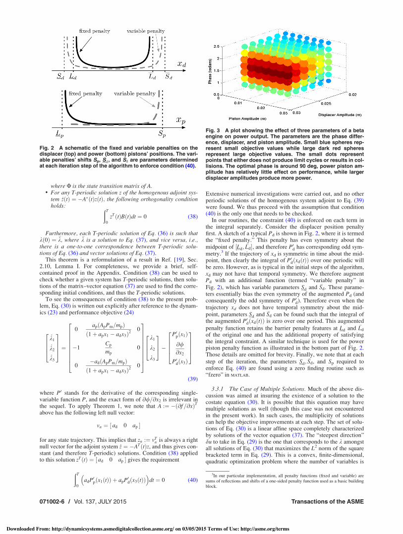
Fig. 2 A schematic of the fixed and variable penalties on thedisplacer (top) and power (bottom) pistons’ positions. The vari-able penalties’ shifts Sp, Sd, and "Sd are parameters determinedat each iteration step of the algorithm to enforce condition (40).

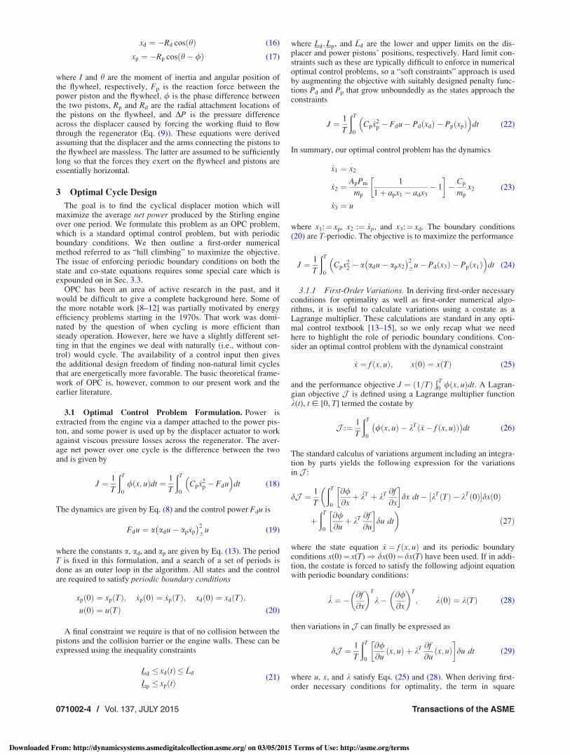
Fig. 3 A plot showing the effect of three parameters of a betaengine on power output. The parameters are the phase differ-ence, displacer, and piston amplitude. Small blue spheres rep-resent small objective values while large dark red spheresrepresent large objective values. The small dots representpoints that either does not produce limit cycles or results in col-lisions. The optimal phase is around 90 deg, power piston am-plitude has relatively little effect on performance, while largerdisplacer amplitudes produce more power.

3In our particular implementation, all penalty functions (fixed and variable) aresums of reflections and shifts of a one-sided penalty function used as a basic buildingblock.

071002-6 / Vol. 137, JULY 2015 Transactions of the ASME

Downloaded From: http://dynamicsystems.asmedigitalcollection.asme.org/ on 03/05/2015 Terms of Use: http://asme.org/terms

precisely the number of linearly independent solutions ofEq. (30).

3.4 Summary of the Algorithm. The hill climbing methodwith periodicity enforcement is now summarized. The followingprocedure is done for each fixed periodic T. The procedure isinitialized by choosing a suitable starting control input u0 (e.g., asinusoid), simulating the open-loop dynamics over several cyclesuntil a steady-state periodic solution is reached. This provides theinitializing trajectories (u0, x0) for Eq. (30).

Steps 1 and 2 below are repeated iteratively within two loops.The innermost loop repeats the steps until no significant improve-ment in the performance objective is observed. The outermostloop then “tightens” the penalty functions, i.e., increases thesteepness of the penalty functions (c.f., Fig. 2) so that these softconstraints effectively enforce the hard limits (21).

(1) Given (un, xn), solve Eq. (30) for kn. This requires the fol-lowing steps.

(2) Using a zero finding routine, determine parameters Sd; "Sd,and Sp to ensure condition (40) for the augmented penalty

functions is satisfied. This guarantees the existence of a per-iodic solution to the costate equations.

(3) Solve the costate equation (30). This is done by solvingEq. (35) for the initial condition "k that will yield a periodicsolution. The state transition matrix and input in Eq. (35)refer to the system (39).

(4) Calculate unþ 1 using Eq. (31), and then xnþ 1 is found bysimulating Eq. (32) until a periodic steady-state is reached.The step size e is chosen small enough to insure improve-ment in the objective function and to avoid collisions.

4 Case Studies

The optimization framework discussed in the pervious sectionwas applied to a Stirling engine model where the displacer pistonmotion is the control input, and a performance comparison with astandard kinematically linked Stirling engine was performed. Wechose a so-called beta-type engine as a benchmark case for com-parison. Such an engine has several design parameters that needto be chosen for satisfactory performance. An importantconsideration is that a fair comparison should be done to a “well-designed” benchmark case. Since there are currently no univer-sally agreed-upon standardized Stirling engine designs, we havechosen to parametrically optimize a beta-type engine to serve asour benchmark reference. Other basic parameters of the enginesthat are not to be optimized (such as reservoir temperatures,cylinder areas, and nominal pressure) are taken from Ref. [7].

4.1 Benchmark: Parametrically Optimized Beta Engine.The benchmark engine used is the beta model described in

Sec. 2.2. This engine has several design parameters including theflywheel and its kinematic linkages /, Rp, Rd, and I. A standardnonlinear programming method of optimization was applied toobtain the parameter values producing the maximum averagepower over one engine cycle. The objective function used was Eq.(18), with the term accounting for power loss from displaceractuation removed. It was found that changing I served mainly tochange the time needed for the engine to reach steady-state, buthad little effect on the resulting power produced at steady-state.Therefore, I was chosen as constant and not a parameter in theoptimization routine. The constraints were that the radii must bepositive, while being small enough to prevent collisions with the

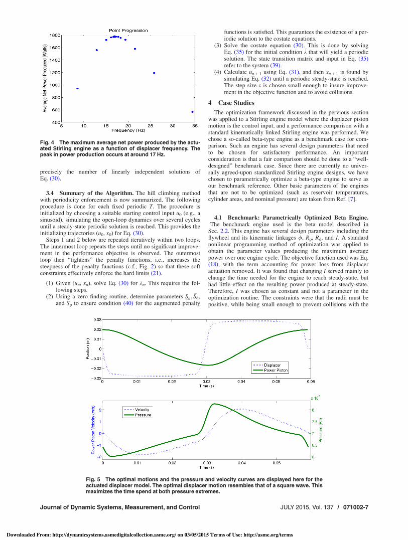
Fig. 4 The maximum average net power produced by the actu-ated Stirling engine as a function of displacer frequency. Thepeak in power production occurs at around 17 Hz.

Fig. 5 The optimal motions and the pressure and velocity curves are displayed here for theactuated displacer model. The optimal displacer motion resembles that of a square wave. Thismaximizes the time spend at both pressure extremes.

Journal of Dynamic Systems, Measurement, and Control JULY 2015, Vol. 137 / 071002-7

Downloaded From: http://dynamicsystems.asmedigitalcollection.asme.org/ on 03/05/2015 Terms of Use: http://asme.org/terms

engine wall and the collision barrier. The fmincon routine inMATLAB was used to find the optimal radii and the phase differ-ence. The function called by fmincon simulated the beta enginegiven the radii and phase differences. Once the engine reachedsteady-state, the function returned the rate of power extraction tofmincon.

Figure 3 shows the engine’s net mechanical power output as afunction of the three design variables. This figure illustrates thatpower output is relatively insensitive to power piston amplitude,while optimal phase is close to 90 deg, and that larger displacer

piston motions (limited by constraints that avoid collisions)produce higher power.

4.2 Performance With Optimal Cycle Design. The periodicoptimal control algorithm was used to optimize the operating cycleof a displacer-actuated version of the parametrically optimized betaengine. For a range of operating frequencies, the algorithm wasexecuted and Fig. 4 shows the resulting maximum average netpower as a function of frequency. The maximum average net powerproduced was just under 1800 W at approximately 17 Hz.

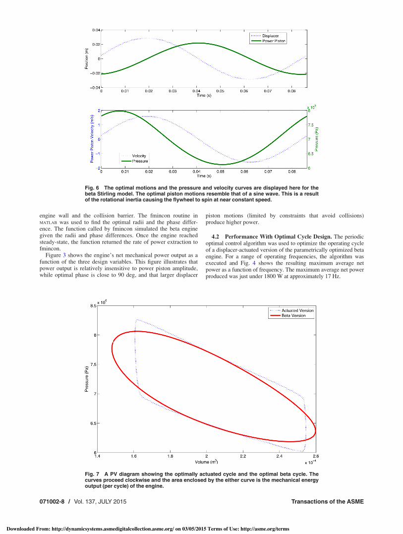
Fig. 6 The optimal motions and the pressure and velocity curves are displayed here for thebeta Stirling model. The optimal piston motions resemble that of a sine wave. This is a resultof the rotational inertia causing the flywheel to spin at near constant speed.

Fig. 7 A PV diagram showing the optimally actuated cycle and the optimal beta cycle. Thecurves proceed clockwise and the area enclosed by the either curve is the mechanical energyoutput (per cycle) of the engine.

071002-8 / Vol. 137, JULY 2015 Transactions of the ASME

Downloaded From: http://dynamicsystems.asmedigitalcollection.asme.org/ on 03/05/2015 Terms of Use: http://asme.org/terms

At the frequency corresponding to maximum net power, opti-mal displacer and power piston trajectories are shown in Fig. 5.Note that displacer motion is closer to a square wave than a puresinusoid; this maximizes the time spent at the two pressureextremes (c.f., Fig. 5), and thus impulses applied to the power pis-ton will be maximized and minimized in the appropriate direc-tions. This intuitively shows how maximum power is transferredto the power piston. The two piston trajectories appear to beapproximately 90 deg out of phase, though it is a little difficult tounambiguously measure phase shifts for nonsinusoidal signals.We note, however, that this phase shift is an outcome of the opti-mization rather than being enforced with kinematic linkages as isthe case in traditional Stirling engines.

For comparison, the optimal displacer and power piston trajec-tories for the beta model are shown in Fig. 6. Note how thesemotions resemble those of a pure sinusoid; this is primarily aresult of the rotational inertia of the flywheel causing it to spin atnear constant speed.

Finally, the pressure/volume (PV) diagrams for both the betaand optimally actuated models are shown in Fig. 7. The areasenclosed by the two models are very similar in size, so they pro-duce roughly the same energy per cycle. However, the operatingfrequency of the actuated model is faster than that of the betamodel (as can be seen when comparing Figs. 5 and 6), so it com-pletes more cycles in a given amount of time. The end result isthat the optimally actuated model produces 42% more power thanthe optimally designed beta model.

A natural question is what the performance of the beta enginewould be if operated at the faster frequency that is optimal for theactuated engine? However, in order to insure a valid comparisonbetween the two engines, the only changes which can be made tothe beta engine design are those used in the construction of the fly-wheel; thus, this is the only way the operating frequency can beadjusted. Since the flywheel parameters were already optimizedfor maximum average net power, any alteration to their valueswould result in decreased performance.

5 Conclusions

We have shown how the framework of OPC can be used todesign optimal cycles for displacer-actuated Stirling engines. Theperformance objective is the net power harvested by the enginefrom the heat reservoirs’ temperature difference. Both the optimalengine’s cycling frequency as well as the optimal piston motionwaveforms are obtained as a result of the optimization. The opti-mal waveforms show significant higher harmonic content, and dis-placer piston motions in particular are closer to square waves thanthey are to pure sinusoids. The operating frequencies are also dif-ferent from those that result from optimized kinematic linkages. Acase study was presented where an optimally actuated engine pro-duced 42% more mechanical power than a comparable, best-case-design kinematically linked engine.

This work is a starting point for the use of OPC for actuatedStirling engine optimization. One of the major drawbacks of theisothermal Schmidt model is the assumption of instantaneous heattransfer from the external reservoirs to the working gas. Currentwork includes the application of the OPC framework presentedhere to higher fidelity models of the Stirling engine which incor-porate finite-rate heat transfer, as well as more detailed models ofregenerator dynamics. We expect that OPC would be even morecritical and beneficial in these more complex models.

On a more general note, it is likely that OPC is the properframework for a large class of energy conversion and harvestingproblems. Cyclic operation is natural in such problems, and whenactive actuation is introduced, the role of OPC is to find more en-ergetically favorable limit cycles than the ones that would occurnaturally without active actuation. We have demonstrated thisidea for a simple Stirling engine model in the present work, butwe believe this basic framework to be applicable to several otherenergy conversion problems as well.

Acknowledgment

This work was partially supported by the NSF CMMI-1363386.

Appendix

Existence of Periodic Solutions to PeriodicallyTime-Varying Systems

The equivalence of the first and second clause of Theorem 1 isa simple argument that was outlined in the text leading toEq. (35). It remains to show the equivalence of the second andthird clauses.

Considering the matrix–vector equation (37) and recall two fun-damental facts from linear algebra. A matrix–vector equation ofthe form

M"k ¼ w

has a solution "k if and only if (iff) the vector w is in the range (col-umn span) of the matrix M, i.e., w 2 RðMÞ. The second fact isthat for any matrix, its range and the null space of its adjoint areorthogonal and complementary, i.e.,

RðMÞ ? N ðMTÞ

This means that w 2 RðMÞ iff it is perpendicular to every elementof the null space of MT, i.e.,

w 2 RðMÞ , 8"zs:t:MT"z ¼ 0; "zTw ¼ 0 (A1)

Now applying this to the matrix–vector equation (37), we see thatthe condition MT"z ¼ 0 amounts to I $ UTðT; 0Þ

( )"z ¼ 0. The latter

statement is equivalent to

"z ¼ UTðT; 0Þ"z , UTð0;TÞ"z ¼ "z

since UTðT; 0Þ( )$1¼ UTð0;TÞ. It is well known that

Ua(T, 0)¼UT(0, T) is the state transition matrix of the adjointsystem

_zðtÞ ¼ $ATðtÞzðtÞ (A2)

and therefore the statement UTð0;TÞ"z ¼ "z is equivalent to theexistence of a T-periodic solution of the system (A2) withzð0Þ ¼ zðTÞ ¼ "z. Finally, we rewrite the dot product term "zTw inEq. (A1) as applied to Eq. (37)

"zT

ðT

0

UðT; tÞBðtÞdt ¼ðT

0

UTðT; tÞ"z( )T

BðtÞdt

and observe that the function UTðT; :Þ"z ¼ Uað:;TÞ"z is simply thesolution of Eq. (A2) with the final boundary condition zðTÞ ¼ "z,therefore a T-periodic solution.

In summary, applying the fundamental linear algebra result(A1) to the system (37) gives the following: for all "z such thatUTð0;TÞ"z ¼ "z (i.e., for all periodic solutions z(.) of Eq. (A2)), wemust have:

ðT

0

zTðtÞBðtÞdt ¼ 0

which is the second clause of the theorem.

References[1] Kongtragool, B., and Wongwises, S., 2003, “A Review of Solar-Powered Stir-

ling Engines and Low Temperature Differential Stirling Engines,” RenewableSustainable Energy Rev., 7(2), pp. 131–154.

Journal of Dynamic Systems, Measurement, and Control JULY 2015, Vol. 137 / 071002-9

Downloaded From: http://dynamicsystems.asmedigitalcollection.asme.org/ on 03/05/2015 Terms of Use: http://asme.org/terms

[2] Riofrio, J. A., Al-Dakkan, K., Hofacker, M. E., and Barth, E. J., 2008,“Control-Based Design of Free-Piston Stirling Engines,” American ControlConference, IEEE, pp. 1533–1538.

[3] Hofacker, M., Kong, J., and Barth, E. J., 2009, “A Lumped-Parameter DynamicModel of a Thermal Regenerator for Free-Piston Stirling Engines,” ASME Pa-per No. DSCC2009-2741, pp. 237–244.

[4] Hofacker, M. E., Tucker, J. M., and Barth, E. J., 2011, “Modeling and Valida-tion of Free-Piston Stirling Engines Using Impedance Controlled Hardware-in-the-Loop,” ASME Paper No. DSCC2011-6105, pp. 153–160.

[5] Mueller-Roemer, C., and Caines, P., 2013, “Isothermal Energy Function State.Space Model of a Stirling Engine,” ASME J. Dyn. Syst., Meas., Control(Submitted).

[6] Gopal, V. K., Duke, R., and Clucas, D., 2009, “Active Stirling Engine,” TEN-CON 2009-2009 IEEE Region 10 Conference, IEEE, pp. 1–6.

[7] Ulusoy, N., 1994, “Dynamic Analysis of Free Piston Stirling Engines,” Ph.D.thesis, Case Western Reserve University, Cleveland, OH.

[8] Speyer, J., and Evans, R., 1984, “A Second Variational Theory for Optimal Per-iodic Processes,” IEEE Trans. Autom. Control, 29(2), pp. 138–148.

[9] Speyer, J. L., Dannemiller, D., and Walker, D., 1985, “Periodic Optical Cruiseof an Atmospheric Vehicle,” J. Guid. Control Dyn., 8(1), pp. 31–38.

[10] Speyer, J. L., 1996, “Periodic Optimal Flight,” J. Guid. Control Dyn., 19(4), pp.745–755.

[11] Gilbert, E. G., 1976, “Vehicle Cruise: Improved Fuel Economy by PeriodicControl,” Automatica, 12(2), pp. 159–166.

[12] Gilbert, E. G., 1977, “Optimal Periodic Control: A General Theory of Neces-sary Conditions,” SIAM J. Control Optim., 15(5), pp. 717–746.

[13] Sage, A. P., 1968, “Optimum Systems Control,” Technical Report DTIC Document.[14] Bryson, A. E., and Ho, Y.-C., 1975, Applied Optimal Control: Optimization,

Estimation, and Control, Taylor & Francis, Boca Raton, FL.[15] Kirk, D. E., 2012, Optimal Control Theory: An Introduction, Dover Publica-

tions, Mineola, NY.[16] Horn, F., and Lin, R., 1967, “Periodic Processes: A Variational Approach,” Ind.

Eng. Chem. Process Des. Dev., 6(1), pp. 21–30.[17] Kowler, D. E., and Kadlec, R. H., 1972, “The Optimal Control of a Periodic

Adsorber: Part II. Theory,” AIChE J., 18(6), pp. 1212–1219.[18] van Noorden, T., Verduyn Lunel, S., and Bliek, A., 2003, “Optimization of Cycli-

cally Operated Reactors and Separators,” Chem. Eng. Sci., 58(18), pp. 4115–4127.[19] Yakubovich, V., and Starzhinskii, V., 1972, Lineinye differentsial’nye uravne-

niya s periodicheskimi koeffitsientami (Linear Differential Equations WithPeriodic Coefficients), Wiley, New York.

071002-10 / Vol. 137, JULY 2015 Transactions of the ASME

Downloaded From: http://dynamicsystems.asmedigitalcollection.asme.org/ on 03/05/2015 Terms of Use: http://asme.org/terms