Optimal Payout Ratio under Perfect Market and Uncertainty: Theory and Empirical Evidence

Cheng-Few Lee Rutgers University

Janice H. Levin Building Piscataway, N.J. 08854-8054

E-mail: lee@business.rutgers.edu

Manak C. Gupta Temple University

428 Alter Hall Fox School of Business Philadelphia, PA 19122

E-mail: mcgupta@temple.edu

Hong-Yi Chen Rutgers University

E-mail: hchen37@pegasus.rutgers.edu

Alice C. Lee* State Street Corp., Boston, MA, USA

E-mail: alice.finance@gmail.com

February 2010

* Disclaimer: Any views or opinions presented in this publication are solely those of the authors and do not necessarily represent those of State Street Corporation. State Street Corporation is not associated in any way with this publication and accepts no liability for the contents of this publication.

1

Optimal Payout Ratio under Perfect Market and Uncertainty: Theory and Empirical Evidence

Abstract

The main purpose of this paper is to develop a theoretical model of the optimal

payout ratio under perfect markets and uncertainty. First, we theoretically derive the

proposition of DeAngelo and DeAngelo’s (2006) optimal payout policy when a partial

payout is allowed. Second, we theoretically derive the impact of total risk, systematic

risk, and growth rate on the optimal payout ratio.

We use the U.S. data during 1969 to 2008 to investigate the impact of total risk,

systematic risk, and growth rate on the optimal payout ratio. We find that the

relationship between the payout ratio and risk is negative (or positive) when the growth

rate is higher (or lower) than the rate of return on assets. In addition, we also find that a

company will generally reduce its payout when the growth rate increases.

2

Optimal Payout Ratio under Perfect Market and Uncertainty: Theory and Empirical Evidence

1. Introduction

Corporate dividend policy has long engaged the attention of financial economists,

dating back to the irrelevance theorem of Miller and Modigliani (1961; M&M) where

they state that there are no illusions in a rational and a perfect economic environment.

Since then, their rather controversial findings have been challenged and tested by

weakening the assumptions and/or introducing imperfections into the analysis. The

signaling models developed by Bhattacharya (1979) and Miller and Rock (1985) have

yielded mixed results. Studies by Nissim and Ziv (2001), Brook et al. (1998), Bernheim

and Wantz (1995), Kao and Wu (1994), and Healy and Palepu (1988) support the

signaling (asymmetric information) hypothesis by finding a positive association between

dividend increases and future profitability. Kalay and Lowenstein (1986) and Asquith

and Mullins (1983) find that dividend changes are positively associated with stock returns

in the days surrounding the dividend announcement dates and Sasson and Kalody (1976)

conclude that there is a positive association between the payout ratio and average rates of

return. On the other hand, studies of Benartzi, Michaely, and Thaler (1997) and

DeAngelo, DeAngelo, and Skinner (1996) find no support for the hypothesized

relationship between dividend changes and future profitability.

Another important factor affecting dividend policy, it is argued, is agency costs

(Easterbrook, 1984; Jensen, 1986). Again, the results of empirical studies have been

mixed at best. Several researchers, among them, Agrawal and Jayaraman (1994), Jensen,

Solberg, and Zorn (1992), and Lang and Litzenberger (1989) find positive support for the

3

agency cost hypothesis, while others find no support for this hypothesis [e.g., Lie (2000),

Yoon and Starks (1995), and Denis et al. (1994)].

Economists have also addressed other possible imperfections as well, such as taxes

and tax-induced clientele effects. Kalay and Michaely (l993), Litzenberger and

Ramaswamy (l979), for example, find positive support while Black and Scholes (l974)

find no such support for a tax-effect hypothesis. Other explanations for market

imperfections range from transactions cost and flotation costs to irrational behavior.

Behavioral theories have recently found increasing attention, among them “avoiding the

regret,” “habit,” and “bounded rationality” explanations for the so-called dividend puzzle.

Lee et al. (1987) have developed a dynamic dividend adjustment model. Besides, there

have been several industry specific studies, for example, Akhigbe et al. (1993), Baker and

Powell (1999) and Gupta and Walker (l975).

DeAngelo and DeAngelo (2006) have reexamined the irrelevance of the M&M

dividend irrelevance theorem by allowing not to pay out all free cash flow. They argue

that the original Miller and Modigliani (1961) irrelevance result is “irrelevant” because it

only considers either paying out all of the free cash flow or not paying any of the free

cash flow, resulting in a sub-optimal payout policy. Therefore, payout policy matters a

great deal if the payout policies under consideration are those in which not all of the free

cash is paid out.

The main purpose of this paper is to develop a theoretical model to support the

proposition of DeAngelo and DeAngelo’s (2006) optimal payout policy when the partial

payout is allowed. In addition, we use an uncertainty instead of a certainty model. By

using this uncertainty model, we derive a theoretical relationship between the optimal

4

ratio and both systematic risk and total risk. The importance of the stochasticity and

nonstationarity of the firm’s profitability in analyzing the effectiveness of dividend policy

is explored in some detail. Furthermore, using assumptions similar to those of DeAngelo

and DeAngelo (2006), we allow the dynamic model holding some amount of cash into a

positive NPV project for financial flexibility reason1. Our dynamic model can show the

existence of an optimal payout ratio under a frictionless market with uncertainty. In

addition, we also explicitly derive the theoretical relationship between the optimal payout

ratio and important financial variables, such as systematic risk and total risk. In other

words, we perform comparative analysis of the relationship between the payout ratio and

(i) change in total risk; (ii) change in systematic risk; (iii) changes in both total risk and

systematic risk, simultaneously; (iv) no change in risk. Our results show that the optimal

payout policy with respect to risk of a firm will depend upon whether its growth rate is

larger or smaller than its rate of return on assets.

Based upon the theoretical model derived in this paper, we implement US data into

empirical analysis. A growing body of empirical research focuses on the optimal

dividend payout policy. For example, Rozeff (1982) shows that optimal dividend payout

is related to the fraction of insider holding, growth of the firm, and the firm’s beta

coefficient. Specifically, he finds evidence that the optimal dividend payout is negatively

correlated to beta risk. Grullon et al. (2002) show that dividend changes are related to the

change in the growth rate and the change in ROA (rate of return on assets). They also

find that dividend increases are associated with subsequent declines in profitability and

1 One of the reviewers points out that some static models have already shown it profit maximizing to allow for financial flexibility [eg. Gabudean (2007), Blau and Fuller, (2008)]. In addition, this reviewer also points out that several empirical study find evidence of firms preferring financial flexibility [eg. Lie, (2005), DeAngelo et al. (2006), and Denis and Osobov, (2007)].

5

risk. Aivazian et al. (2003) examine eight emerging markets and show that, similar to

U.S. firms, dividend policies in emerging markets can also be explained by profitability,

debt, and the market-to-book ratio. However, none of them has a solid theoretical model

to support their finding. Based upon our model, we try to examine the existence of

optimal payout policy among dividend-paying companies. Using U.S. data during the

period 1969 to 2008, we analyze a panel data of 19,774 dividend-paying firm years by

taking advantage of the Fama-MacBeth procedure and the fixed effect regression model.

We find negative risk effects on dividend payout policy among firms with higher growth

rates relative to their expected rate of return on assets.

In section 2, we lay out the basic elements of the stochastic control theory model

that we use in the subsequent sections to examine the existence, or nonexistence, of an

optimal dividend policy. The model assumes a stochastic rate of return and is not

restricted to firms growing entirely through retained earnings. The model is developed in

the most general form assuming a nonstationary profitability rate of the firm and using

the systematic risk concept of risk.

In section 3, we carry out the optimization procedure to maximize firm value.

Therefore, the final expression for the optimal dividend policy of the firm can be derived.

In section 4, the implications of the results are explained. In particular, the separate and

then the combined effects of market dependent and market independent components of

risk on the optimal dividend policy are identified. Also, we examine in detail the effects

of variations in the profitability rate, its distribution parameters, and their dynamic

behavior on the optimal dividend policy of the firm. In section 5, we provide both a

detailed form and an approximated form of our theoretical model in discussion of the

6

relationship between the optimal dividend payout ratio and the growth rate. We also

implement a sensitivity analysis to investigate the relationship between the optimal

payout policy and the growth rate. In section 6, we use U.S. data to provide empirical

evidence supporting the model and implications in previous sections. Using both the

Fama-MacBeth procedure and fixed effect models, the empirical results are consistent

with the implications of our model discussed in sections 4 and 5. Finally, section 7

presents the conclusion.

2. The Model

We develop the dividend policy model under the assumptions that the capital

markets represent the closest approximation to the economists’ ideal of a perfect market –

zero transaction costs, rational behavior on the part of investors, and the absence of tax

differentials between dividends and capital gains. It is assumed that the firm is not

restricted to financing its growth only by retained earnings, and that its rate of return,

( )r t� , is a nonstationary random variable, normally distributed with mean, µ, and

variance, 2( )tσ .

Let ( )A o represent the initial assets of the firm and h be the growth rate. Then, the

earnings of this firm are given by Eq. (1), which is

( ) ( ) ( ) htx t r t A o e=� � , (1)

where ( )x t� represents the earnings of the firm, and the tilde (~) denotes its random

character.

7

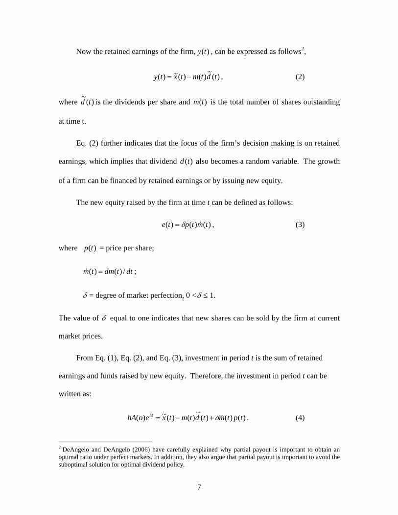
Now the retained earnings of the firm, )(ty , can be expressed as follows2,

)(~

)()(~)( tdtmtxty −= , (2)

where )(~

td is the dividends per share and ( )m t is the total number of shares outstanding

at time t.

Eq. (2) further indicates that the focus of the firm’s decision making is on retained

earnings, which implies that dividend ( )d t also becomes a random variable. The growth

of a firm can be financed by retained earnings or by issuing new equity.

The new equity raised by the firm at time t can be defined as follows:

)()()( tmtpte �δ= , (3)

where )(tp = price per share;

dttdmtm /)()( =� ;

δ = degree of market perfection, 0 <δ ≤ 1.

The value of δ equal to one indicates that new shares can be sold by the firm at current

market prices.

From Eq. (1), Eq. (2), and Eq. (3), investment in period t is the sum of retained

earnings and funds raised by new equity. Therefore, the investment in period t can be

written as:

)()()(~

)()(~)( tptmtdtmtxeohA ht�δ+−= . (4)

2 DeAngelo and DeAngelo (2006) have carefully explained why partial payout is important to obtain an optimal ratio under perfect markets. In addition, they also argue that partial payout is important to avoid the suboptimal solution for optimal dividend policy.

8

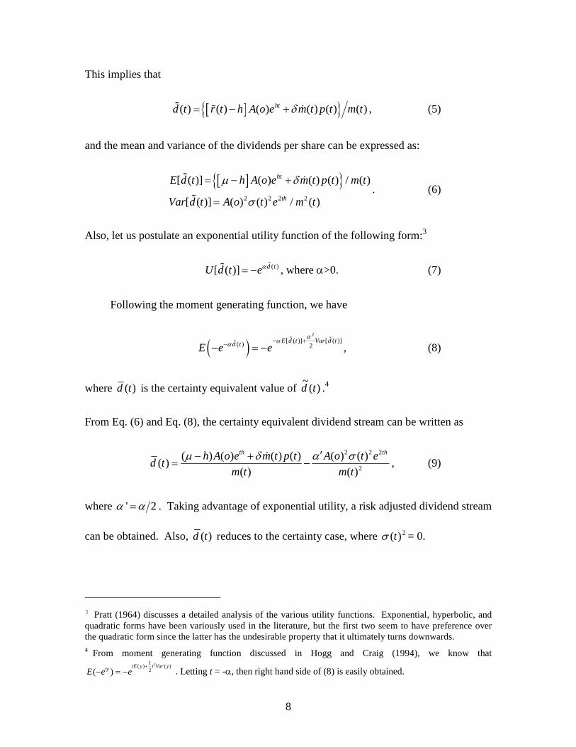
This implies that

[ ]{ }( ) ( ) ( ) ( ) ( ) ( )htd t r t h A o e m t p t m tδ= − +� � � , (5)

and the mean and variance of the dividends per share can be expressed as:

[ ]{ }

2 2 2 2

[ ( )] ( ) ( ) ( ) / ( )

[ ( )] ( ) ( ) / ( )

ht

th

E d t h A o e m t p t m t

Var d t A o t e m t

µ δ

σ

= − +

=

� �

�

. (6)

Also, let us postulate an exponential utility function of the following form:3

( )[ ( )] d tU d t eα= −�

� , where α>0. (7)

Following the moment generating function, we have

( )2

[ ( )] [ ( )]( ) 2E d t Var d td tE e e

ααα − +−− = −

� ��

, (8)

where ( )d t is the certainty equivalent value of )(~

td .4

From Eq. (6) and Eq. (8), the certainty equivalent dividend stream can be written as

2 2 2

2

( ) ( ) ( ) ( ) ( ) ( )( )

( ) ( )

th thh A o e m t p t A o t ed t

m t m t

µ δ α σ′− += −

�, (9)

where ' 2α α= . Taking advantage of exponential utility, a risk adjusted dividend stream

can be obtained. Also, ( )d t reduces to the certainty case, where 2)(tσ = 0.

3 Pratt (1964) discusses a detailed analysis of the various utility functions. Exponential, hyperbolic, and quadratic forms have been variously used in the literature, but the first two seem to have preference over the quadratic form since the latter has the undesirable property that it ultimately turns downwards. 4 From moment generating function discussed in Hogg and Craig (1994), we know that

21( ) ( )

2( )tE y t Var ytyE e e

+− = − . Letting t = -α, then right hand side of (8) is easily obtained.

9

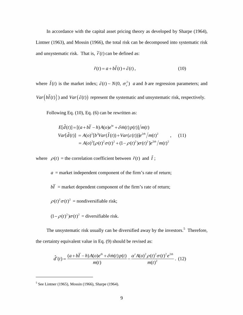
In accordance with the capital asset pricing theory as developed by Sharpe (1964),

Lintner (1963), and Mossin (1966), the total risk can be decomposed into systematic risk

and unsystematic risk. That is, )(~ tr can be defined as:

( ) ( ) ( )r t a bI t tε= + +� �� , (10)

where ( )I t� is the market index; 2( ) (0, )t N εε σ� ∼ a and b are regression parameters; and

( )( )Var bI t� ) and ( )( )Var tε� represent the systematic and unsystematic risk, respectively.

Following Eq. (10), Eq. (6) can be rewritten as:

2 2 2 2

2 2 2 2 2 2 2

[ ( )] [( ) ( ) ( ) ( )] ( )

[ ( )] ( ) [ ( ( )) ( ( ))] ( )

( ) [ ( ) ( ) (1 ( ) ) ( ) ] ( )

ht

th

th

E d t a bI h A o e m t p t m t

Var d t A o b Var I t Var t e m t

A o t t t t e m t

δ

ε

ρ σ ρ σ

= + − +

= +

= + −

� �

� � , (11)

where ( )tρ = the correlation coefficient between ( )r t� and I� ;

a = market independent component of the firm’s rate of return;

bI = market dependent component of the firm’s rate of return;

2 2( ) ( )t tρ σ = nondiversifiable risk;

2 2(1 ( ) ) ( )t tρ σ− = diversifiable risk.

The unsystematic risk usually can be diversified away by the investors.5 Therefore,

the certainty equivalent value in Eq. (9) should be revised as:

2 2 2 2

2

( ) ( ) ( ) ( ) ( ) ( ) ( )ˆ ( )( ) ( )

th tha bI h A o e m t p t A o t t ed t

m t m t

δ α ρ σ′+ − +′ = −�

. (12)

5 See Lintner (1965), Mossin (1966), Sharpe (1964).

10

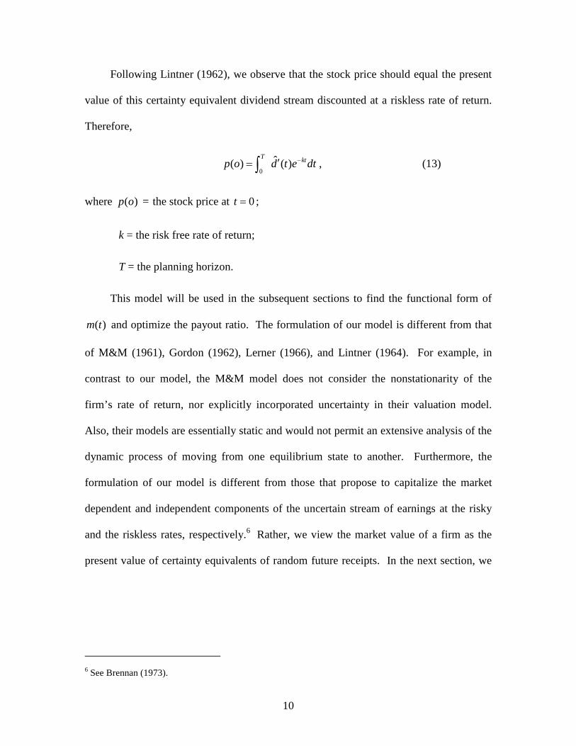
Following Lintner (1962), we observe that the stock price should equal the present

value of this certainty equivalent dividend stream discounted at a riskless rate of return.

Therefore,

0

ˆ( ) ( )T ktp o d t e dt−′= ∫ , (13)

where ( )p o = the stock price at 0t = ;

k = the risk free rate of return;

T = the planning horizon.

This model will be used in the subsequent sections to find the functional form of

( )m t and optimize the payout ratio. The formulation of our model is different from that

of M&M (1961), Gordon (1962), Lerner (1966), and Lintner (1964). For example, in

contrast to our model, the M&M model does not consider the nonstationarity of the

firm’s rate of return, nor explicitly incorporated uncertainty in their valuation model.

Also, their models are essentially static and would not permit an extensive analysis of the

dynamic process of moving from one equilibrium state to another. Furthermore, the

formulation of our model is different from those that propose to capitalize the market

dependent and independent components of the uncertain stream of earnings at the risky

and the riskless rates, respectively.6 Rather, we view the market value of a firm as the

present value of certainty equivalents of random future receipts. In the next section, we

6 See Brennan (1973).

11

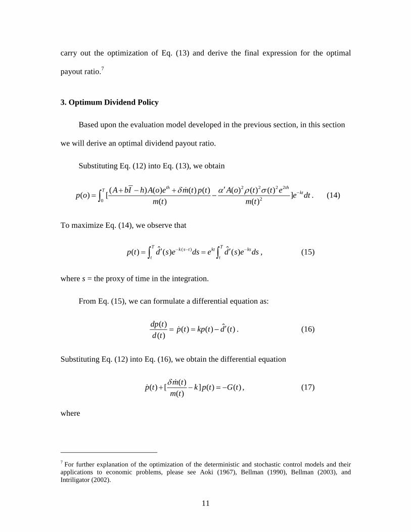
carry out the optimization of Eq. (13) and derive the final expression for the optimal

payout ratio.7

3. Optimum Dividend Policy

Based upon the evaluation model developed in the previous section, in this section

we will derive an optimal dividend payout ratio.

Substituting Eq. (12) into Eq. (13), we obtain

2 2 2 2

20

( ) ( ) ( ) ( ) ( ) ( ) ( )( ) [ ]

( ) ( )

th thT ktA bI h A o e m t p t A o t t e

p o e dtm t m t

δ α ρ σ −′+ − += −∫

�. (14)

To maximize Eq. (14), we observe that

( )ˆ ˆ( ) ( ) ( )T Tk s t kt ks

t tp t d s e ds e d s e ds− − −′ ′= =∫ ∫ , (15)

where s = the proxy of time in the integration.

From Eq. (15), we can formulate a differential equation as:

( ) ˆ( ) ( ) ( )( )

dp tp t kp t d t

d t′= = −� . (16)

Substituting Eq. (12) into Eq. (16), we obtain the differential equation

( )

( ) [ ] ( ) ( )( )

m tp t k p t G t

m t

δ+ − = −�

� , (17)

where

7 For further explanation of the optimization of the deterministic and stochastic control models and their applications to economic problems, please see Aoki (1967), Bellman (1990), Bellman (2003), and Intriligator (2002).

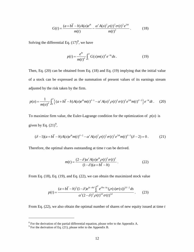
12

2 2 2 2

2

( ) ( ) ( ) ( ) ( )( )

( ) ( )

th tha bI h A o e A o t t eG t

m t m t

α ρ σ′+ −= − . (18)

Solving the differential Eq. (17)8, we have

( ) ( ) ( )( )

ktT ks

t

ep t G s m s e ds

m tδ

δ−= ∫ . (19)

Then, Eq. (20) can be obtained from Eq. (18) and Eq. (19) implying that the initial value

of a stock can be expressed as the summation of present values of its earnings stream

adjusted by the risk taken by the firm.

{ }1 2 2 2 2 2

0

1( ) ( ) ( ) ( ) ( ) ( ) ( ) ( )

( )

T th th ktp o a bI h A o e m t A o t t e m t e dtm o

δ δδ α ρ σ− − −′= + − −∫ . (20)

To maximize firm value, the Euler-Lagrange condition for the optimization of ( )p o is

given by Eq. (21)9,

2 2 2 2 2 3( 1)( ) ( ) ( ) ( ) ( ) ( ) ( ) ( 2) 0th tha bI h A o e m t A o t t e m tδ δδ α ρ σ δ− −′− + − − − = . (21)

Therefore, the optimal shares outstanding at time t can be derived.

2 2(2 ) ( ) ( ) ( )

( )(1 )( )

thA o e t tm t

a bI h

δ α ρ σδ′−

=− + −

. (22)

From Eq. (18), Eq. (19), and Eq. (22), we can obtain the maximized stock value

2 2 2

2 2 2

( ) (1 ) ( ( ) ( ))( )

(2 ) ( ) ( )

Tkt th hs ks

ta bI h e e s s ds

p tt t

δ δ δ

δ δ

δ ρ σ

α δ ρ σ

− − −+ − −=

′ −∫

. (23)

From Eq. (22), we also obtain the optimal number of shares of new equity issued at time t

8 For the derivation of the partial differential equation, please refer to the Appendix A. 9 For the derivation of Eq. (21), please refer to the Appendix B.

13

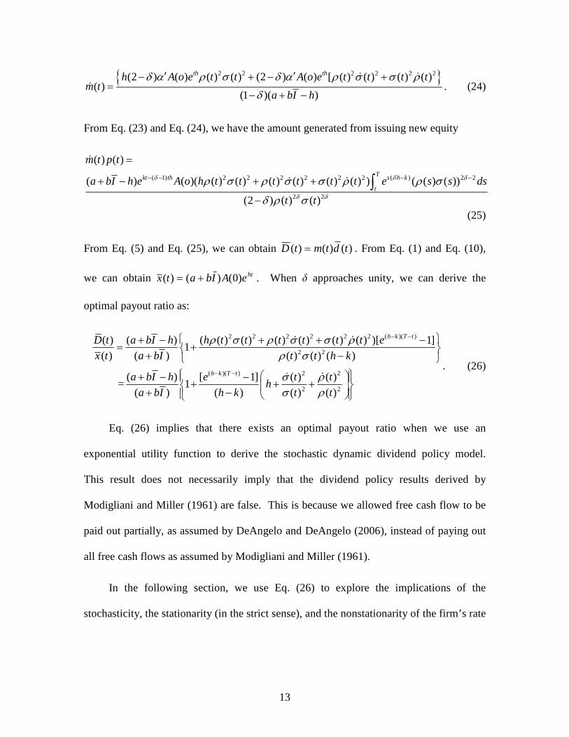
{ }2 2 2 2 2 2(2 ) ( ) ( ) ( ) (2 ) ( ) [ ( ) ( ) ( ) ( )( )

(1 )( )

th thh A o e t t A o e t t t tm t

a bI h

δ α ρ σ δ α ρ σ σ ρ

δ

′ ′− + − +=

− + −

��

� . (24)

From Eq. (23) and Eq. (24), we have the amount generated from issuing new equity

( 1) 2 2 2 2 2 2 ( ) 2 2

2 2

( ) ( )

( ) ( )( ( ) ( ) ( ) ( ) ( ) ( ) ) ( ( ) ( ))

(2 ) ( ) ( )

Tkt th s h k

t

m t p t

a bI h e A o h t t t t t t e s s ds

t t

δ δ δ

δ δ

ρ σ ρ σ σ ρ ρ σ

δ ρ σ

− − − −

=

+ − + +

−∫

�

��

(25)

From Eq. (5) and Eq. (25), we can obtain )()()( tdtmtD = . From Eq. (1) and Eq. (10),

we can obtain hteAIbatx )0()()( += . When δ approaches unity, we can derive the

optimal payout ratio as:

2 2 2 2 2 2 ( )( )

2 2

( )( ) 2 2

2 2

( ) ( ) ( ( ) ( ) ( ) ( ) ( ) ( ) )[ 1]1

( ) ( ) ( ) ( ) ( )

( ) [ 1] ( ) ( ) = 1

( ) ( ) ( ) ( )

h k T t

h k T t

D t a bI h h t t t t t t e

x t a bI t t h k

a bI h e t th

a bI h k t t

ρ σ ρ σ σ ρρ σ

σ ρσ ρ

− −

− −

+ − + + −= +

+ −

+ − − + + + + −

��

��

. (26)

Eq. (26) implies that there exists an optimal payout ratio when we use an

exponential utility function to derive the stochastic dynamic dividend policy model.

This result does not necessarily imply that the dividend policy results derived by

Modigliani and Miller (1961) are false. This is because we allowed free cash flow to be

paid out partially, as assumed by DeAngelo and DeAngelo (2006), instead of paying out

all free cash flows as assumed by Modigliani and Miller (1961).

In the following section, we use Eq. (26) to explore the implications of the

stochasticity, the stationarity (in the strict sense), and the nonstationarity of the firm’s rate

14

�of return for its dividend policy. Also, we investigate in detail the differential effects of

variations in the systematic and unsystematic risk components of the firm’s stream of

earnings on the dynamics of its dividend policy.

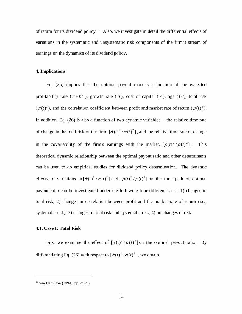
4. Implications

Eq. (26) implies that the optimal payout ratio is a function of the expected

profitability rate (a bI+ ), growth rate (h ), cost of capital (k ), age (T-t), total risk

( 2( )tσ ), and the correlation coefficient between profit and market rate of return ( 2)(tρ ).

In addition, Eq. (26) is also a function of two dynamic variables -- the relative time rate

of change in the total risk of the firm, ])(/)([ 22 tt σσ� , and the relative time rate of change

in the covariability of the firm's earnings with the market, ])(/)([ 22 tt ρρ� . This

theoretical dynamic relationship between the optimal payout ratio and other determinants

can be used to do empirical studies for dividend policy determination. The dynamic

effects of variations in ])(/)([ 22 tt σσ� and ])(/)([ 22 tt ρρ� on the time path of optimal

payout ratio can be investigated under the following four different cases: 1) changes in

total risk; 2) changes in correlation between profit and the market rate of return (i.e.,

systematic risk); 3) changes in total risk and systematic risk; 4) no changes in risk.

4.1. Case I: Total Risk

First we examine the effect of ])(/)([ 22 tt σσ� on the optimal payout ratio. By

differentiating Eq. (26) with respect to ])(/)([ 22 tt σσ� , we obtain

10 See Hamilton (1994), pp. 45-46.

15

( )( )

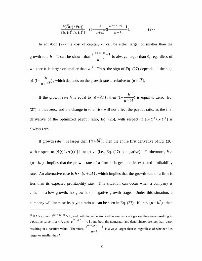
2 2

[ ( ) / ( )] 1(1 )[ ]

[ ( ) / ( ) ]

h k T tD t x t h e

t t a bI h kσ σ

− −∂ −= −

∂ + −�. (27)

In equation (27) the cost of capital, k , can be either larger or smaller than the

growth rate h . It can be shown that ( )( ) 1h k T te

h k

− − −−

is always larger than 0, regardless of

whether k is larger or smaller than h .11 Thus, the sign of Eq. (27) depends on the sign

of (1 )h

a bI−

+, which depends on the growth rate h relative to ( ).a bI+

If the growth rate h is equal to )( Iba + , then )1(Iba

h

+− is equal to zero. Eq.

(27) is thus zero, and the change in total risk will not affect the payout ratio, as the first

derivative of the optimized payout ratio, Eq. (26), with respect to ])(/)([ 22 tt σσ� is

always zero.

If growth rate h is larger than )( Iba + , then the entire first derivative of Eq. (26)

with respect to ])(/)([ 22 tt σσ� is negative (i.e., Eq. (27) is negative). Furthermore, h >

)( Iba + implies that the growth rate of a firm is larger than its expected profitability

rate. An alternative case is h < )( Iba + , which implies that the growth rate of a firm is

less than its expected profitability rate. This situation can occur when a company is

either in a low growth, no growth, or negative growth stage. Under this situation, a

company will increase its payout ratio as can be seen in Eq. (27). If h < )( Iba + , then

11 If h > k, then ( )( ) 1h k T te − − > , and both the numerator and denominator are greater than zero, resulting in

a positive value; if h < k, then 1))(( <−− tTkhe , and both the numerator and denominator are less than zero,

resulting in a positive value. Therefore, ( )( ) 1h k T te

h k

− − −

− is always larger than 0, regardless of whether k is

larger or smaller than h.

16

Eq. (27) is positive, indicating that a relative increase in the risk of the firm would

increase its optimal payout ratio. This implies that a relative increase in the total risk of

the firm would decrease its optimal payout ratio. Both Lintner (1965) and Blau and

Fuller (2008) have found this kind of relationship. However, they did not theoretically

show how this kind of relationship can be derived.

Jagannathan et al. (2000) empirically show that operation risk is negatively

related to the propensity to increase payouts in general and dividends in particular. Our

theoretical analysis in terms of Eq. (27) shows that the change in total risk is negatively

or positively related to the payout ratio, conditional on the growth rate relative to the

expected profitability rate.

We find negative relationships between payout and the change in total risk for high

growth firms (h > )( Iba + ). The possible explanation is that in the case of high growth

firms, a firm needs to reduce the payout ratio and retain more earnings to build up

“precautionary reserves.” These reserves become all the more important for a firm with

volatile earnings over time. In addition, the age of the firm (T-t), which is one of the

variables in Eq. (27), becomes an important factor because the very high growth firms are

also the newer firms with very little built-up precautionary reserves. Furthermore, these

high growth firms need more retained earnings to meet their future growth opportunities

since the growth rate is the main determinant of value in the case of such companies.

In the case of established low growth firms (h < )( Iba + ), such firms are likely to

be more mature and most likely already built such reserves over time. In addition, they

17

probably do not need more earnings to maintain their low growth perspective and can

afford to increase the payout.

Thus, we provide, under more dynamic conditions, further evidence on the validity

of Lintner’s (1965) observations that, ceteris paribus, optimal dividend payout ratios vary

directly with the variance of the firm's profitability rates. The rationale for such

relationships, even when the systematic risk concept is incorporated into the analysis, is

obvious. That is, holding 2)(tρ constant and letting the 2)(tσ increase implies that the

covariance of the firm's earnings with the market does not change though its relative

proportion to the total risk increases.

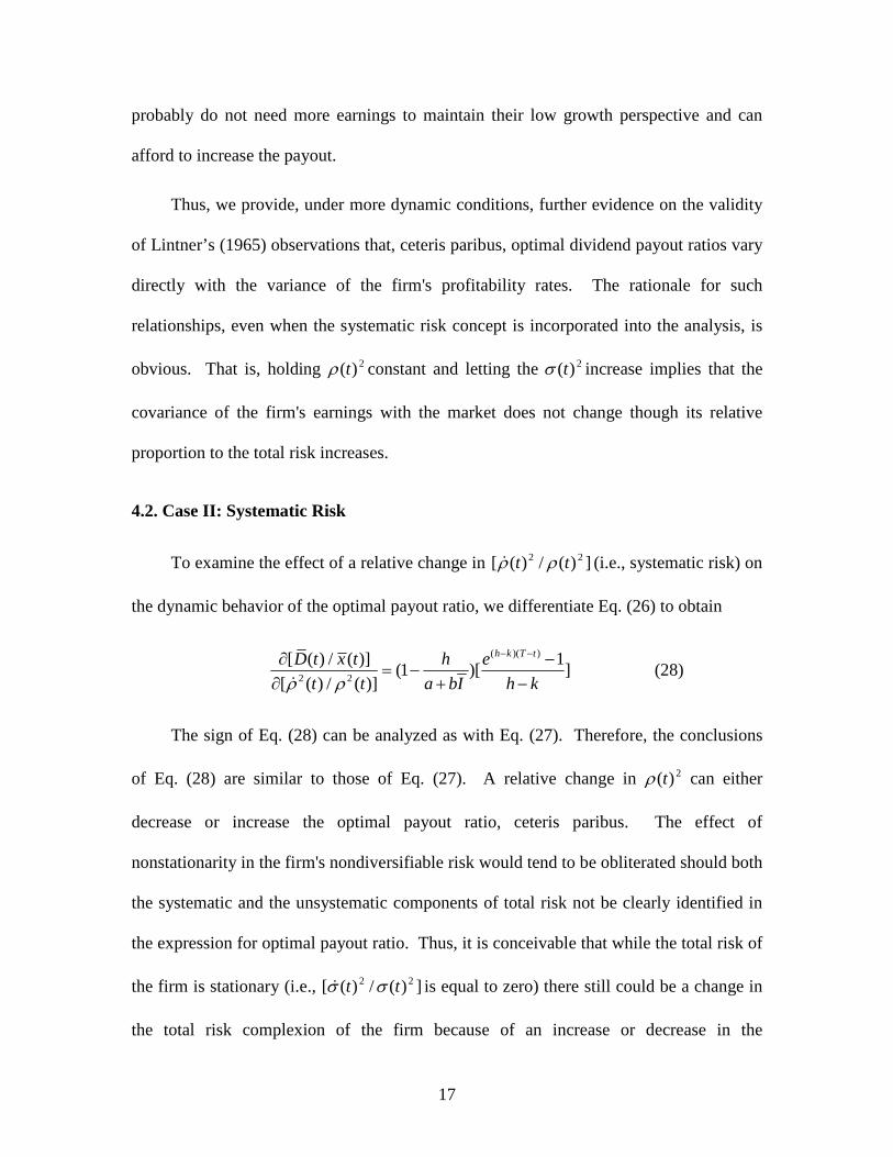
4.2. Case II: Systematic Risk

To examine the effect of a relative change in ])(/)([ 22 tt ρρ� (i.e., systematic risk) on

the dynamic behavior of the optimal payout ratio, we differentiate Eq. (26) to obtain

( )( )

2 2

[ ( ) / ( )] 1(1 )[ ]

[ ( ) / ( )]

h k T tD t x t h e

t t a bI h kρ ρ

− −∂ −= −

∂ + −� (28)

The sign of Eq. (28) can be analyzed as with Eq. (27). Therefore, the conclusions

of Eq. (28) are similar to those of Eq. (27). A relative change in 2)(tρ can either

decrease or increase the optimal payout ratio, ceteris paribus. The effect of

nonstationarity in the firm's nondiversifiable risk would tend to be obliterated should both

the systematic and the unsystematic components of total risk not be clearly identified in

the expression for optimal payout ratio. Thus, it is conceivable that while the total risk of

the firm is stationary (i.e., ])(/)([ 22 tt σσ� is equal to zero) there still could be a change in

the total risk complexion of the firm because of an increase or decrease in the

18

covariability of its earnings with the market. Eq. (26) and Eq. (28) clearly identify the

effect of such a change in the risk complexion of the firm on its optimal payout ratio.

Furthermore, an examination of Eq. (26) indicates that only when the firm’s

earnings are perfectly correlated with the market (i.e., 2ρ = 1), it does not matter whether

the management arrives at its optimal payout ratio using the total variance concept of risk

or the market concept of risk. For every other case, the optimal payout ratio followed by

management using the total variance concept of risk would be an overestimate of the true

optimal payout ratio for the firm based on the market concept of risk underlying the

capital asset pricing theory.

Also, the management may decide not to use the truly dynamic model and instead

substitute an average of the long run systematic risk of the firm. However, for )(2 tρ� > 0,

it is evident that since the average initially is higher than the true )(2 tρ , the management

would be paying out less or more in the form of dividends than is optimal. That is, the

payout ratio followed in the initial part of the planning horizon would be an overestimate

or an underestimate of the optimal payout under truly dynamic specifications.

Rozeff (1982) empirically shows a negative relationship between the β coefficient

(systematic risk) and the payout level. The theoretical analysis in terms of Eq. (28) gives

a more detailed analytical interpretation of his findings. The explanations of these results

are similar to those discussed for Jagannathan et al’s (2000) findings in previous sections.

4.3. Case III: Total Risk and Systematic Risk

In our third case, we attempt to investigate the compounded effect of a

simultaneous change in the total risk of the firm and also a change in its decomposition

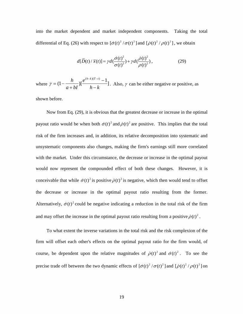
19

into the market dependent and market independent components. Taking the total

differential of Eq. (26) with respect to ])(/)([ 22 tt σσ� and ])(/)([ 22 tt ρρ� , we obtain

2 2

2 2

( ) ( )[ ( ) / ( )] ( ) ( )

( ) ( )

t td D t x t d d

t t

σ ργ γ

σ ρ= +

��, (29)

where ]1

)[1())((

kh

e

bIa

h tTkh

−−

+−=

−−

γ . Also, γ can be either negative or positive, as

shown before.

Now from Eq. (29), it is obvious that the greatest decrease or increase in the optimal

payout ratio would be when both 2)(tσ� and 2)(tρ� are positive. This implies that the total

risk of the firm increases and, in addition, its relative decomposition into systematic and

unsystematic components also changes, making the firm's earnings still more correlated

with the market. Under this circumstance, the decrease or increase in the optimal payout

would now represent the compounded effect of both these changes. However, it is

conceivable that while 2)(tσ� is positive 2)(tρ� is negative, which then would tend to offset

the decrease or increase in the optimal payout ratio resulting from the former.

Alternatively, 2)(tσ� could be negative indicating a reduction in the total risk of the firm

and may offset the increase in the optimal payout ratio resulting from a positive 2)(tρ� .

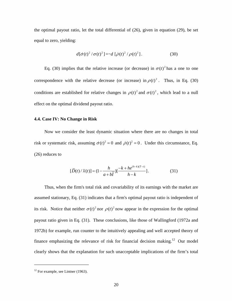
To what extent the inverse variations in the total risk and the risk complexion of the

firm will offset each other's effects on the optimal payout ratio for the firm would, of

course, be dependent upon the relative magnitudes of 2)(tρ� and 2)(tσ� . To see the

precise trade off between the two dynamic effects of ])(/)([ 22 tt σσ� and ])(/)([ 22 tt ρρ� on

20

the optimal payout ratio, let the total differential of (26), given in equation (29), be set

equal to zero, yielding:

d ])(/)([ 22 tt σσ� =−d ])(/)([ 22 tt ρρ� . (30)

Eq. (30) implies that the relative increase (or decrease) in 2)(tσ has a one to one

correspondence with the relative decrease (or increase) in 2)(tρ . Thus, in Eq. (30)

conditions are established for relative changes in 2)(tρ and 2)(tσ , which lead to a null

effect on the optimal dividend payout ratio.

4.4. Case IV: No Change in Risk

Now we consider the least dynamic situation where there are no changes in total

risk or systematic risk, assuming 2( ) 0tσ =� and 2( ) 0tρ =� . Under this circumstance, Eq.

(26) reduces to

( )( )

[ ( ) / ( )] (1 )[ ]h k T th k he

D t x ta bI h k

− −− += −

+ −. (31)

Thus, when the firm's total risk and covariability of its earnings with the market are

assumed stationary, Eq. (31) indicates that a firm's optimal payout ratio is independent of

its risk. Notice that neither 2)(tσ nor 2)(tρ now appear in the expression for the optimal

payout ratio given in Eq. (31). These conclusions, like those of Wallingford (1972a and

1972b) for example, run counter to the intuitively appealing and well accepted theory of

finance emphasizing the relevance of risk for financial decision making.12 Our model

clearly shows that the explanation for such unacceptable implications of the firm’s total

12 For example, see Lintner (1963).

21

risk and its market dependent and market independent components for the firm’s optimal

payout policy lies, of course, in the totally unrealistic stationarity assumptions underlying

the derivation of such results as illustrated in Eq. (31).

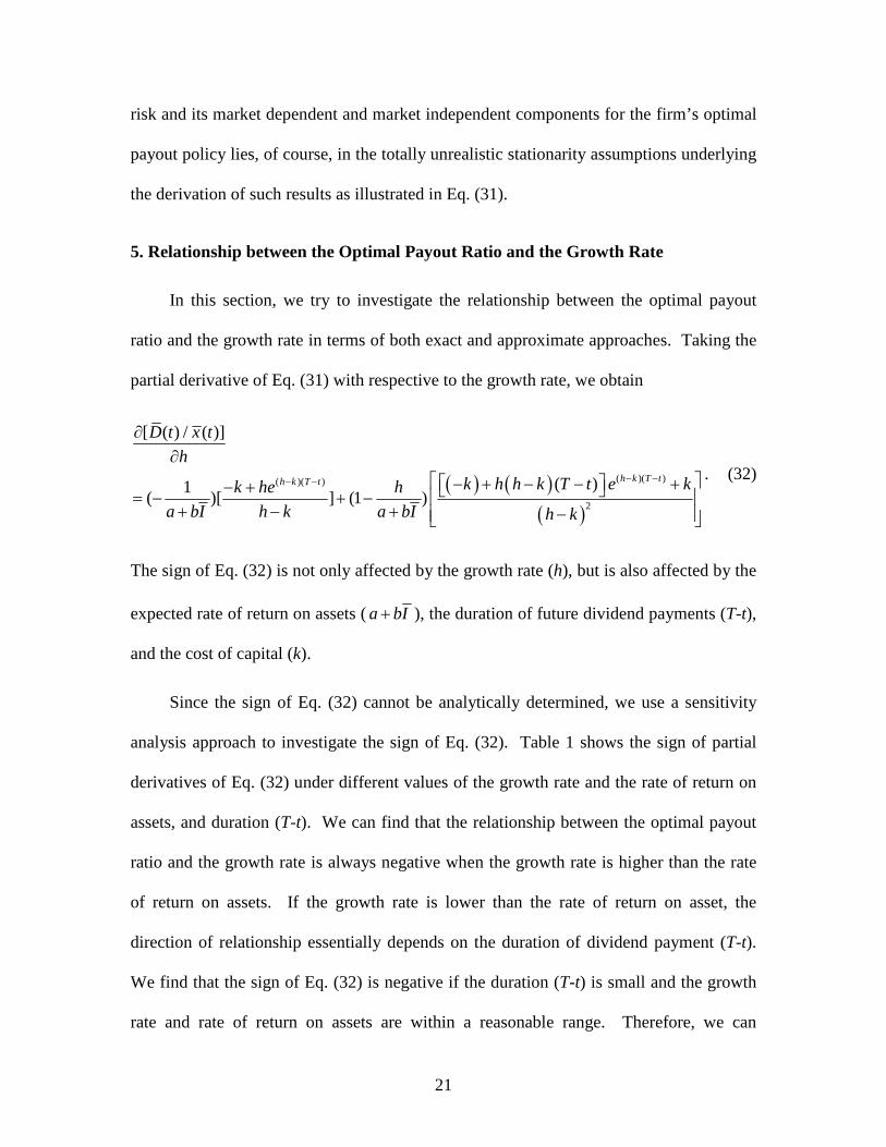
5. Relationship between the Optimal Payout Ratio and the Growth Rate

In this section, we try to investigate the relationship between the optimal payout

ratio and the growth rate in terms of both exact and approximate approaches. Taking the

partial derivative of Eq. (31) with respective to the growth rate, we obtain

( ) ( )( )

( )( )( )( )

2

[ ( ) / ( )]

( )1( )[ ] (1 )

h k T th k T t

D t x t

h

k h h k T t e kk he h

a bI h k a bI h k

− −− −

∂∂

− + − − +− + = − + − + − + −

. (32)

The sign of Eq. (32) is not only affected by the growth rate (h), but is also affected by the

expected rate of return on assets (a bI+ ), the duration of future dividend payments (T-t),

and the cost of capital (k).

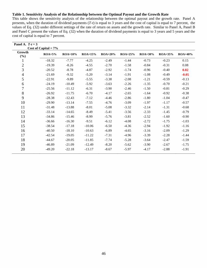
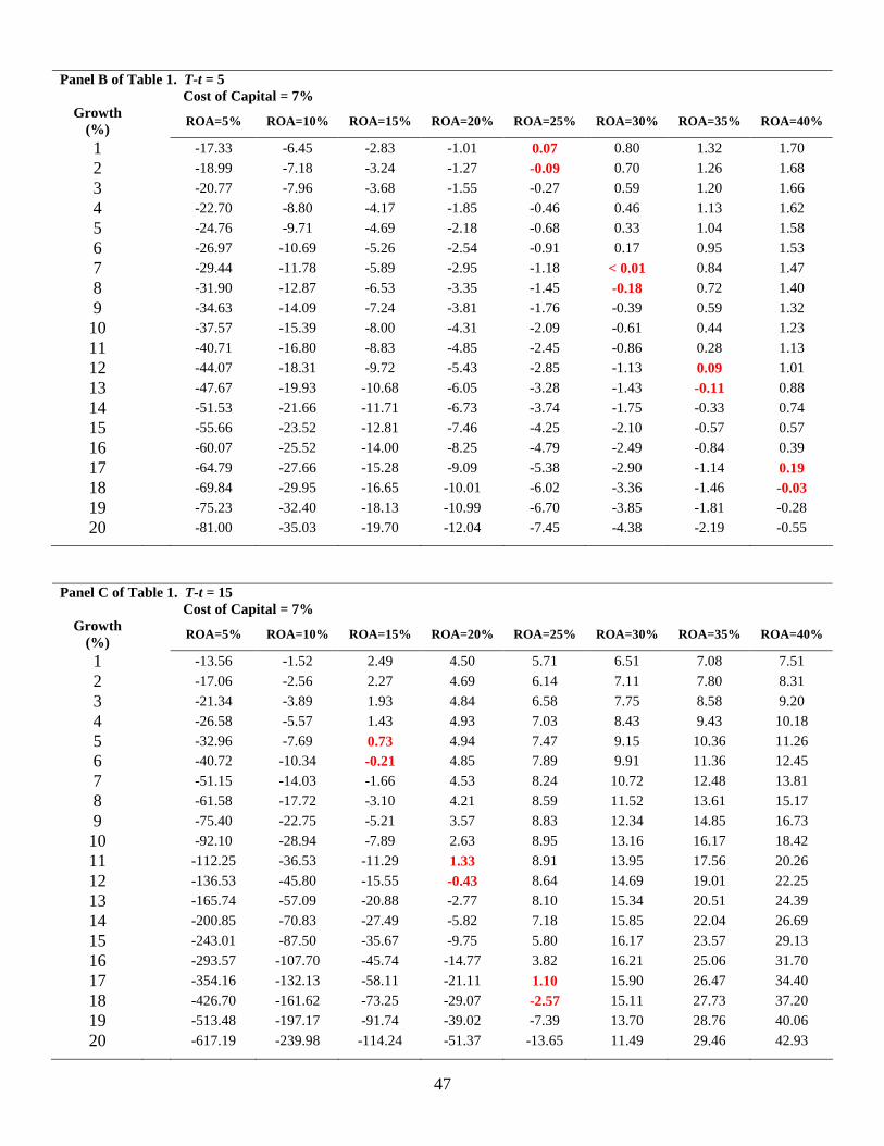
Since the sign of Eq. (32) cannot be analytically determined, we use a sensitivity

analysis approach to investigate the sign of Eq. (32). Table 1 shows the sign of partial

derivatives of Eq. (32) under different values of the growth rate and the rate of return on

assets, and duration (T-t). We can find that the relationship between the optimal payout

ratio and the growth rate is always negative when the growth rate is higher than the rate

of return on assets. If the growth rate is lower than the rate of return on asset, the

direction of relationship essentially depends on the duration of dividend payment (T-t).

We find that the sign of Eq. (32) is negative if the duration (T-t) is small and the growth

rate and rate of return on assets are within a reasonable range. Therefore, we can

22

conclude that the relationship between the optimal payout ratio and the growth rate is

generally negative.

Based upon Eq. (32), Figure 1 plots the change in the optimal payout ratio with

respect to the growth rate in different durations of dividend payments and costs of capital.

We can find a negative relationship between the optimal payout ratio and the growth rate

indicating that a firm with a higher rate of return on assets tends to payout less when its

growth opportunities increase. Moreover, a firm with a lower growth rate and higher

expected rate of return will not decrease its payout when its growth opportunities increase.

However, a firm with a lower growth and a higher expected rate of return on asset is not a

general case in the real world. Furthermore, we also find that the duration of future

dividend payments is also an important determinant of the dividend payout decision,

while the effect on the cost of capital is relatively minor.

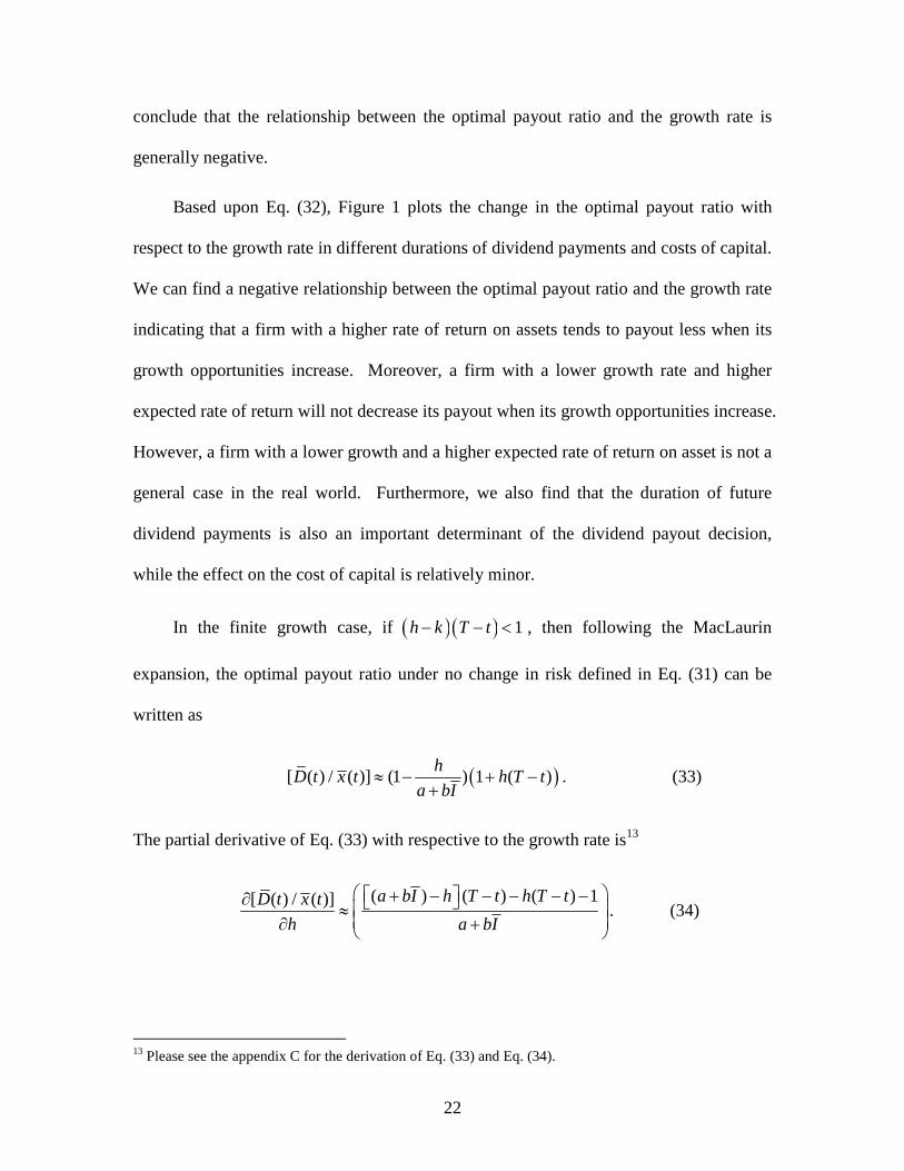
In the finite growth case, if ( )( ) 1h k T t− − < , then following the MacLaurin

expansion, the optimal payout ratio under no change in risk defined in Eq. (31) can be

written as

( )[ ( ) / ( )] (1 ) 1 ( )h

D t x t h T ta bI

≈ − + −+

. (33)

The partial derivative of Eq. (33) with respective to the growth rate is13

( ) ( ) ( ) 1[ ( ) / ( )] a bI h T t h T tD t x t

h a bI

+ − − − − −∂ ≈ ∂ +

. (34)

13 Please see the appendix C for the derivation of Eq. (33) and Eq. (34).

23

Eq. (34) indicates that the relationship between the optimal dividend payout and the

growth rate depends on firm’s level of growth, the rate of return on assets, and the

duration of future dividend payment. Eq. (34) is negative when the rate of return on asset

is lower than the growth rate. This implies that firm will reduce its payout when its

growth rate increases. The higher growth rate (h) and the lower rate of return on asset

( a bI+ ) will lead to a more negative relationship between dividend payout ratio and

growth rate. More specifically, the condition of Eq. (35) will lead to a negative

relationship between the optimal payout ratio and the growth rate.

1 1

( )2 ( )

h a bIT t

> + − −

. (35)

Therefore, consistent with the sensitivity analysis of Eq. (32), when a firm with a high

growth rate or a low rate of return on assets faces a growth opportunity, it will decrease

its dividend payout to generate more cash to meet such a new investment.

In this section we have shown that, in general cases, the relationship between the

optimal payout ratio and the growth rate is negative. In the next section, we will

investigate the impact of risks and growth rate on the optimal payout ratio.

6. Empirical Evidence

A growing body of literature focuses on the determinants of optimal dividend

payout policy. For example, Rozeff (1982) shows that the optimal dividend payout is

related to the fraction of insider holdings, the growth of the firm, and the firm’s beta

coefficient. He also finds evidence that the optimal dividend payout is negatively

correlated to beta risk supporting that beta risk reflects the leverage level of a firm.

24

Grullon et al. (2002) show that dividend changes are related to the change in the growth

rate and the change in the rate of return on assets. They also find that dividend increases

should be associated with subsequent declines in profitability and risk. Aivazian et al.

(2003) examine eight emerging markets and show that, similar to U.S. firms, dividend

policies in emerging markets can also be explained by profitability, debt, and the

market-to-book ratio. However, none of them considers the growth rate and the

expected rate of return at the same time. Based upon our model, we here try to examine

the existence of an optimal payout policy among dividend-paying companies. Our

prediction is that the optimal payout policy will differ from differing levels of growth

rate with respect to their expected rate of return.

6.1. Sample Description

We collect from Compustat the firm information including total asset, sales, net

income, and dividends payout, etc. Stock price, stock returns, share codes, and exchange

codes are retrieved from the Center for Research in Security Prices (CRSP) files. The

sample period is from 1969 to 2008. Only common stocks (SHRCD = 10, 11) and firms

listed on NYSE, AMEX, or NASDAQ (EXCE = 1, 2, 3, 31, 32, 33) are included in our

sample. We exclude utility services (SICH = 4900-4999) and financial institutions

(SICH = 6000-6999)14. The sample includes those firm-years with at least five years of

data available to compute average payout ratios, growth rate, return on assets, beta, total

risk, size, and book-to-market ratios. The payout ratio is measured as the ratio of the

14 We filter out those financial institutions and utility firms based on historical SIC code (SICH) available from COMPUSTAT. When a firm’s historical SIC code is unavailable for a particular year, the next available historical SIC code is applied instead. When a firm’s historical SIC code is unavailable for a particular year and all the years after, we use current SIC code (SIC) from COMPUSTAT as a substitute.

25

dividend payout to the net income. The growth rate is the sustainable growth rate

proposed by Higgins (1977). The beta coefficient and total risk are estimated by the

market model over the previous 60 months. For the purpose of estimating their betas,

firm-years in our sample should have at least 60 consecutive previous monthly returns.

To examine the optimal payout policy, only firm-years with five consecutive dividend

payouts are included in our sample15. Considering the fact that firm-years with no

dividend payout one year before (or after) might not start (or stop) their dividend payouts

in the first (fourth) quarter of the year, we exclude firm-years with no dividend payouts

one year before or after from our sample to ensure the dividend payout policy reflects

firm’s full-year condition.

Table 2 shows the summary statistics for 1,895 sample firms during the period year

1969 and year 2008. Panel A of Table 2 lists the number of firm-year observations for all

sample, high growth firms, and low growth firms respectively. High growth firm-years

are those firm-years that have five-year average sustainable growth rates higher than their

five-year average rate of return on assets. Low growth firm-years are those firms with

five-year average sustainable growth lower than their five-year average rate of return on

assets. The sample size increases from 325 firms in 1969 to 804 firms in 1982, while

declining to 353 firms by 2008. There are a total of 19,744 dividend paying firm-years in

the sample. When classifying into high growth firms and low growth firms relative to

their return on assets, the proportion of high growth firms is increasing with time. The

15 To avoid making large difference in dividend policy, managers usually partially adjust firms’ payout by several years to reduce the sudden impacts of the changes in dividend policy. On the other hand, managers also base on not only one year firm conditions but also multi-year firm conditions to decide how much they will payout. Therefore, in examining the optimal payout policy, we use the 5-year rolling averages for all variables.

26

proportion of firm-years with a growth rate higher than return on assets increases from

less than 50 percent during late 1960s and early 1970s to 90 percent in 2008. Panel B of

Table 2 shows the five-year moving averages of mean, median, and standard deviation

values for the measures of payout ratio, growth rate, rate of return, beta coefficient, total

risk, market capitalization, and market-to-book ratio across all firm-years in the sample.

Among high growth firms, the average growth rate is 12.87 percent and the average

payout ratio is 31.87 percent, while for low growth firms, the average growth rate is 5.14

percent and the average payout ratio is 56.04 percent. The finding of lower payout ratio

in high growth firms is consistent with the agency cost of cash flow hypothesis (e.g.

Fama and French (2001), Grullon et al. (2002), and DeAngelo and DeAngelo (2006)) that

firms with less investment opportunities will pay more dividends to reduce the free cash

flow agency problem. Moreover, high growth firms undertake more beta risk and total

risk indicating that high growth firms undertake both more systematic risk and

unsystematic risk to pursue a higher rate of return.

Table 2 shows that a firm’s dividend payout policy depends on its growth rate

relative to its return on assets, and firms can increase their risk-taking to maintain in high

growth level. Therefore, the linkages from dividend payouts to growth rate, from growth

rate to risks offer a venue for the analysis of the relationship between dividend payout

policy and risk based on firm’s growth rate. In the following analyses, we will examine

how a firm’s growth rate with respect to its expected rate of return on assets affects the

relationship between the payout ratio and risk.

27

6.2. Multivariate Analysis

To examine the relationship between the payout ratio and risks, we propose a cross-

sectional model of the payout ratio on risk measures (beta coefficient and total risk). In

the regression, the logistic transformation of the payout ratio is to convert an otherwise

bounded dependent variable into an unbounded one. Control variables include the

growth rate, size, and market-to-book ratio. The cross-sectional regression is defined as

follows.

( ) 1 2 3

ln _ ln( )

1 i

i i ii

payout ratioRisk Growth Option Size e

payout ratioα β β β

= + + + + −

(36)

Rozeff (1982), Fenn and Liang (2001), Grullon et al. (2002), Aivazian et al. (2003),

and Blau and Fuller (2008) find a negatively related risk effect on the dividend payout.

Firm’s risks are affected by its financial risk resulting from financial leverage. When a

firm faces higher financial risk, it will decrease its payout ratio to save more cash for

possible future interest payments and financial flexibility reason. However, previous

studies do not consider that different levels of growth rate may result in a different

relationship between the firm’s payout and its risks. Our theoretical model shows that the

correlation between risk and the payout ratio depends on the firm’s growth rate relative to

its expected rate of return on assets. Therefore, we expect a mixed result for the

estimated coefficient (1β ) in multivariate regressions when pooling high growth and low

growth firms together, though a negative 1β is observed in previous studies.

Rozeff (1982) and Fama and French (2001) point that firms with high growth

opportunities will tend to pay less (or not pay) dividend, while Fenn and Liang (2001)

28

propose a mixed effect for growth options on payout policy. They suggest that high

growth firms not only face more profitable opportunities but also greater uncertainties.

With greater uncertainties, firms require a more flexible payout policy and, hence, rely

more heavily on repurchases than dividends. Thus, the expected signs of the proxies for

the growth option (e.g. sustainable growth rate, sales growth, market-to-book ratio, and

rate of return on assets) are mixed.

Smith and Watts (1992) and Opler and Titman (1993) show that large firms have

more stable cash flows and less information asymmetries, allowing them to have lower

financing costs. With stable cash flows and lower costs of financing, large firms can

payout more dividends than small firms. Therefore, the sign of estimated coefficient for

size is positive.

Table 3 provides the results of Fama-MacBeth regressions for 1,895 firms during

the period 1969 to 2008. Panel A shows the relationship between the payout ratio and

beta risk. The estimated regression coefficients of beta risk are all negative during the

entire 40 year period, and the average value of the regression coefficients of beta risk is -

0.66 with a t-statistics of -21.41. The average value of the regression coefficients of total

risk is -44.06 with a t-statistics of -13.66. Panel B shows a similar result that the payout

ratio is negatively correlated to total risk. The results are similar to the findings of Rozeff

(1982), Jagannathan et al. (2000), and Grullon et al. (2002) that dividend payouts are

negatively correlated to firm risks. However, our model shows that, if firms follow their

optimal dividend payout policy, the relationship between dividend payouts and firm risks

depends on their growth rates relative to their rate of return on assets. From Table 2, we

find the number of firms with a higher growth rate with respect to their rate of return on

29

assets is greater than the number of firms with a lower growth rate with respect to their

rates of return on assets. When pooling high growth firms and low growth firms together,

the risk effect of high growth firms will dominate that of low growth firms due to the

larger proportion of high growth firms in the observations. Therefore, the negative risk

effect on dividend payout shown in Table 3 may be due to the greater proportion of high

growth firms. Based on our subsequent analysis, the effect of growth rates on dividend

payout policies can be more accurately found when firms are separated into high growth

firms and low growth firms relative to their rates of return on assetsrate of return on

assets.

Table 3 also provides significantly negative estimators of the growth rate16 which is

consistent with the argument of Rozeff (1982) and Fama and French (2001) that high

growth firms will have higher investment opportunities and tend to pay out less in

dividends. Our findings do not support Fenn and Liang’s (2001) point of view that high

growth firms have greater uncertainties and they rely more heavily on repurchases than

dividends to obtain a more flexible payout policy. In the multiple regressions, we also

find a positive relationship between the payout ratio and firm size, indicating that large

firms can pay more dividends due to their more stable cash flow and lower cost of

financing.

16 The control variable of growth options used in Table 2 is the sustainable growth rate. We also implement other proxies of growth options (e.g. sales growth, book-to-market ratio, and return on asset) and get similar results to those using sustainable the growth rate. The unpresented results are available upon request.

30

6.3. Fama-MacBeth Analysis

To separate the effect of different growth rates relative to the expected rates of

return on assets, we introduce a product of a dummy variable and risk as an interaction

term in the cross-sectional regression. The dummy variable is equal to 1 if a firm’s five-

year average growth rate is greater than its five-year average rate of return on assets and 0

otherwise. Such a structure allows us to analyze separate effects of high growth and low

growth firms on the payout ratio. The regression model is defined as follows.

( )( )1 2

3 4

ln

1

_ ln( )

ii i

i

i i

payout ratioRisk D low growth Risk

payout ratio

Growth Option Size e

α β β

β β

= + + ⋅ −

+ + +

(37)

Table 4 presents the results of cross-sectional regression with dummy variable in

each year. In Panel A of Table 4, the regression coefficient of beta represents the beta

risk effect on the payout ratio for firms with a higher growth rate relative to their rate of

return on assets. During the period from 1969 to 2008, the estimated regression

coefficients of beta are significantly negative at the 1% level in each year. Also the time

series average is -0.57, which is also statistically significant at the 1% level. The

estimated coefficient of the interaction term represents the additional beta risk effect on

the payout ratio for lower growth firms. Results show that the estimated coefficient of

the interaction term is significantly positive at the 1% level in each year and the time

series average is 1.02, which is also statistically significant at the 1% level. A significant

and positive coefficient of additional beta risk effect indicates that, when beta risk

increases, low growth firms will not adjust their dividend payouts as high growth firms

do. By summing the coefficient of beta risk and the coefficient of interaction term, we

31

can obtain a time series average of 0.45 indicating the total beta risk effect for low

growth firms is positive. That is, when beta risk increases, low growth firm will follow

its optimal payout policy to increase its dividend payout ratio. Panel B of Table 4 shows

the results that high growth firms have a significantly negative total risk effect on the

payout ratio, while low growth firms have a significantly positive total risk effect.

Therefore, Table 4 supports the prediction of our model that firms’ payout policies are

affected by their risks. Thus we can conclude that optimal payout policy has a negative

relationship between firm risk and dividend payout among high growth firms and a

positive relationship among low growth firms. Because risk is usually associated with

the level of financial leverage, higher financial leverage results in higher risks. Therefore,

different risk effects on the payout policy can be explained by the fact that growth firms

usually decrease their dividend payouts to save cash to meet the burdens of higher

financial leverage.

6.4. Fixed Effect Analysis

Petersen (2006) points to the drawbacks of using OLS on panel data analysis

because the residuals may be correlated across firms or across time resulting in the OLS

standard errors being biased and significant test results being incorrect. He suggests that

a fixed effect model may solve the potential bias of standard errors. When analyzing the

relationship between the dividend payout and risks, there might be some unobserved

variables omitted in cross-sectional regression model. Such omitted variable effects will

be left in the error term leading to a potential bias of standard errors. Moreover, dividend

payout policy may alter with the years. It is reasonable for a firm to payout less during a

recession period and pay out more in good times. Although the Fama-MacBeth

32

procedure has an adjustment on the potential problem of year effect, it does not deal with

the potential problem of firm effect. In this section, instead of Fama-MacBeth procedure,

we introduce a fixed firm effect to control unobserved firm characteristics and year

effects to control the time effect, which affects a firm’s optimal dividend payout policy.

Table 5 provides results of the panel data analysis on firm’s dividend payout policy

by different models. Model 1 and Model 2 are the summary from Fama-MacBeth

procedures presented in Table 4. Model 3 and Model 4 are one-way fixed year effect

regressions, and Model 5 and Model 6 are one-way fixed firm effect regressions. Model

7 and Model 8 are two-way fixed effect regressions, controlling for both firm effect and

year effect. After controlling for firm effect and year effect, there still exists a

significantly positive risk effect on the payout ratio for high growth firms, and a

significantly negative risk effect on the payout ratio for low growth firms. Therefore, the

empirical results of the fixed effect models also support the prediction in our model that

the relationship between the payout policy and firm risks depends on a firm’s growth rate

relative to its expected rate of return on assets.

Moreover, the impact of the risk effect for high growth firms is also similar to that

of the Fama-MacBeth procedure. Especially when the fixed firm effects are taken into

account, the risk effect is found to have a lower impact on lower growth firms. The

finding of a lower risk effect for low growth firms indicates that low growth firms have a

higher potential problem of standard error bias. Therefore, the risk effect for low growth

firms will be subtracted by some unobserved specific characteristics belonging to firms.

This finding also support the argument of Petersen (2006) that the Fama-MacBeth

33

procedure can deal with the potential problem of year effects, but fail to deal with the

problem of firm effect.

7. Summary and Concluding Remarks

In this paper, the optimal payout ratio is derived by using an exponential utility

function. The results vary from those of the M&M model since their model is stationary

and does not allow for uncertainty and partial payouts of earnings. Also, our dynamic

model presented in this paper allows holding some amount of cash for positive NPV

projects.

Our theoretical model supports the proposition of DeAngelo and DeAngelo’s (2006)

optimal payout policy when a partial payout is allowed. In addition, we use an

uncertainty instead of a certainty model to derive a theoretical relationship between the

optimal ratio and both systematic risk and total risk. Our dynamic model can show the

existence of an optimal payout ratio under a frictionless market with uncertainty. We

also explicitly derive the theoretical relationship between the optimal payout ratio and

important financial variables, such as systematic risk and total risk. We perform a

comparative analysis between the payout ratio and the following: (i) change in total risk;

(ii) change in systematic risk; (iii) change in total risk and systematic risk, simultaneously;

(iv) no change in risk. We also provide a theoretical model to investigate the relationship

between the optimal dividend payout ratio and the growth rate. A sensitivity analysis and

an approximation form can help us to find a negative relationship between the optimal

dividend payout ratio and the growth rate in general.

34

Finally, we also use the data between 1969 and 2008 of 1,895 firms to test the

theoretical propositions which we have derived in this paper. Our empirical results find

that the optimal dividend payout ratio is negatively related to the growth rate. In addition,

the optimal dividend payout ratio is negatively (positively) related to both total risk and

systematic risk when the growth rate is higher (lower) than the rate of return on assets.

Therefore, these empirical results support the theoretical results which we have derived in

this paper.

35

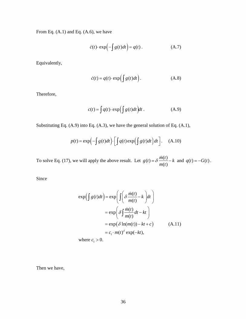
Appendix A. Derivation of Equation (19)

This appendix presents a detailed derivation of the solution to the variable partial

differential equation, Eq. (17), which is similar to Gould’s (1968) Equation (9). in

investigation the adjustment cost. Following Gould’s (1968) approach, we first derive a

general solution for a standard variable partial differential equation. Then we apply this

general equation to solve Eq. (17). The standard variable partial differential equation can

be defined as

( ) ( ) ( ) ( )p t g t p t q t+ =� (A.1)

As a particular case of Eq. (A.1), the equation

( ) ( ) ( ) 0p t g t p t+ =� or ( )

( )( )

p tg t

p t= −

� (A.2)

has a solution

( )( ) exp ( )p t c g t dt= ⋅ −∫ . (A.3)

By substituting constant c with function ( )c t , we have the potential solution to Eq. (A.1)

( )( ) ( ) exp ( )p t c t g t dt= ⋅ −∫ . (A.4)

Taking a differential with respect to t , we obtain

( ) ( )( )

( ) ( ) exp ( ) ( ) exp ( ) ( )

( ) exp ( ) ( ) ( )

p t c t g t dt c t g t dt g t

c t g t dt p t g t

= ⋅ − − ⋅ −

= ⋅ − −

∫ ∫

∫

� �

�

(A.5)

Therefore,

( )( ) ( ) ( ) ( ) exp ( )p t p t g t c t g t dt+ = ⋅ −∫� � . (A.6)

36

From Eq. (A.1) and Eq. (A.6), we have

( )( ) exp ( ) ( )c t g t dt q t⋅ − =∫� . (A.7)

Equivalently,

( )( ) ( ) exp ( )c t q t g t dt= ⋅ ∫� . (A.8)

Therefore,

( )( ) ( ) exp ( )c t q t g t dt dt= ⋅∫ ∫ . (A.9)

Substituting Eq. (A.9) into Eq. (A.3), we have the general solution of Eq. (A.1),

( ) ( )( ) exp ( ) ( )exp ( )p t g t dt q t g t dt dt = − ⋅ ∫ ∫ ∫ . (A.10)

To solve Eq. (17), we will apply the above result. Let ( )

( )( )

m tg t k

m tδ= −�

and ( ) ( )q t G t= − .

Since

( )

( )

1

1

( )exp ( ) exp

( )

( ) exp

( )

exp ln( ( ))

( ) exp( ),

where 0.

m tg t dt k dt

m t

m tdt kt

m t

m t kt c

c m t kt

c

δ

δ

δ

δ

= −

= −

= − +

= ⋅ −

>

∫ ∫

∫

�

�

(A.11)

Then we have,

37

2 3

2 3

( ) ( ) exp( ) ( ) ( ) exp( ) ,

where 0, and 0

P t c m t kt q t c m t kt dt

c c

δ δ− = ⋅ ⋅ ⋅ − > >

∫ (A.12)

or equivalently,

4

4

e ( )( ) ( ) ,

( )

where 0.

kt

kt

m tP t c G t dt

m t e

c

δ

δ

= ⋅ ⋅ −

>

∫ (A.13)

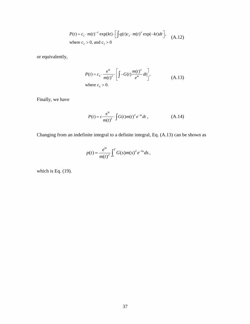
Finally, we have

e

( ) ( ) ( )( )

ktkt

kP t c G t m t e dt

m tδ −= ⋅ ∫ , (A.14)

Changing from an indefinite integral to a definite integral, Eq. (A.13) can be shown as

( ) ( ) ( )( )

ktT ks

t

ep t G s m s e ds

m tδ

δ−= ∫ ,

which is Eq. (19).

38

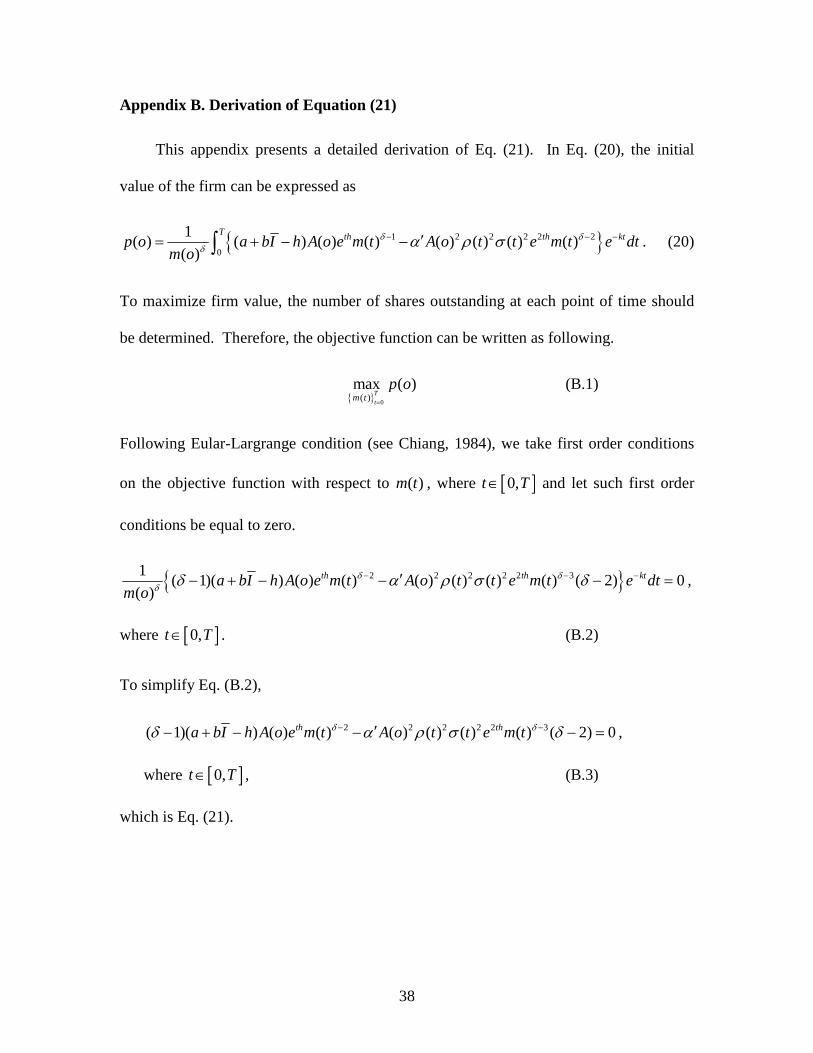
Appendix B. Derivation of Equation (21)

This appendix presents a detailed derivation of Eq. (21). In Eq. (20), the initial

value of the firm can be expressed as

{ }1 2 2 2 2 2

0

1( ) ( ) ( ) ( ) ( ) ( ) ( ) ( )

( )

T th th ktp o a bI h A o e m t A o t t e m t e dtm o

δ δδ α ρ σ− − −′= + − −∫ . (20)

To maximize firm value, the number of shares outstanding at each point of time should

be determined. Therefore, the objective function can be written as following.

{ } 0

( )max ( )

Tt

m tp o

=

(B.1)

Following Eular-Largrange condition (see Chiang, 1984), we take first order conditions

on the objective function with respect to ( )m t , where [ ]0,t T∈ and let such first order

conditions be equal to zero.

{ }2 2 2 2 2 31( 1)( ) ( ) ( ) ( ) ( ) ( ) ( ) ( 2) 0

( )th th kta bI h A o e m t A o t t e m t e dt

m oδ δ

δ δ α ρ σ δ− − −′− + − − − = ,

where [ ]0,t T∈ . (B.2)

To simplify Eq. (B.2),

2 2 2 2 2 3( 1)( ) ( ) ( ) ( ) ( ) ( ) ( ) ( 2) 0th tha bI h A o e m t A o t t e m tδ δδ α ρ σ δ− −′− + − − − = ,

where [ ]0,t T∈ , (B.3)

which is Eq. (21).

39

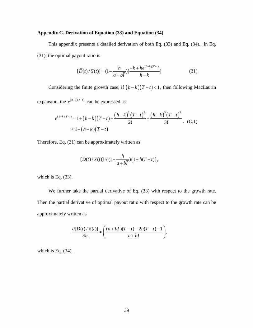
Appendix C. Derivation of Equation (33) and Equation (34)

This appendix presents a detailed derivation of both Eq. (33) and Eq. (34). In Eq.

(31), the optimal payout ratio is

( )( )

[ ( ) / ( )] (1 )[ ]h k T th k he

D t x ta bI h k

− −− += −

+ − (31)

Considering the finite growth case, if ( )( ) 1h k T t− − < , then following MacLaurin

expansion, the ( )( )h k T te − − can be expressed as

( )( ) ( )( ) ( ) ( ) ( ) ( )

( )( )

2 2 3 3

12! 3!

1

h k T t h k T t h k T te h k T t

h k T t

− − − − − −= + − − + +

≈ + − −

. (C.1)

Therefore, Eq. (31) can be approximately written as

( )[ ( ) / ( )] (1 ) 1 ( )h

D t x t h T ta bI

≈ − + −+

,

which is Eq. (33).

We further take the partial derivative of Eq. (33) with respect to the growth rate.

Then the partial derivative of optimal payout ratio with respect to the growth rate can be

approximately written as

[ ( ) / ( )] ( )( ) 2 ( ) 1D t x t a bI T t h T t

h a bI

∂ + − − − −≈ ∂ +

,

which is Eq. (34).

40

References

[1] Agrawal, A. and N. Jayaraman. The dividend policies of all-equity firms: a direct

test of the free cash flow theory. Managerial and Decision Economics, 15, 139-

148, 1994.

[2] Akhigbe, A., S. F. Borde, and J. Madura. Dividend policy and signaling by

insurance companies. Journal of Risk and Insurance, 60, 413-428, 1993.

[3] Asquith, P. and D. Mullins. The impact of initiating dividend payments on

shareholders’ wealth. Journal of Business, 56, 77-96, 1983.

[4] Aivazian, V., L. Booth, S. Cleary. Do emerging market firms follow different

dividend policies from US firms? Journal of Financial Research, 26, 371-387,

2003.

[5] Aoki, M. Optimization of stochastic systems. New York: Academic Press, 1967.

[6] Baker, H., and G. E. Powell, How corporate managers view dividend policy.

Quarterly Journal of Business and Economics, 38, 17-35, 1999.

[7] Bhattacharya, S. Imperfect information, dividend policy, and “the bird in the hand”

fallacy. Bell Journal of Economics, 10, 259-270, 1979.

[8] Bellman, R. Dynamic Programming. Dover Publication, 2003.

[9] Bellman, R. Adaptive Control Process: A Guided Tour. Princeton, N. J.: Princeton

University Press, 1990.

[10] Benartzi, S., R. Michaely, and R. Thaler. Do changes in dividends signal the future

or the past? Journal of Finance, 52, 1007–1034, 1997.

[11] Bernheim, B., and A. Wantz. A tax based test of the dividend signaling hypothesis.

American Economic Review, 85, 532–551, 1995.

[12] Black, F., and M. Scholes, The effect of dividend yield and dividend policy on

common stock prices and returns. Journal of Financial Economics, Vol. I, 1974.

41

[13] Blau, B.M., and K.P. Fuller. Flexibility and Dividends. Journal of Corporate

Finance, 14, 133-152, 2008.

[14] Brennan, M. J. An approach to the valuation of uncertain income stream. Journal

of Finance, 28, 1973.

[15] Brennan, M. J. An inter-temporal approach to the optimization of dividend policy

with predetermined investments: Comment. Journal of Finance, 29, 258–259,

1974.

[16] Brook, Y., W.T. Charlton, and Robert, and R.J. Hendershott. Do firms use

dividends to signal large future cash flow increases? Financial Management,

27, 46-57, 1998.

[17] Chiang, A.C, Fundamental Methods of Mathematical Economics, 3rd Ed, McGraw-

Hill, Inc, NY, 1984.

[18] DeAngelo, H., L. DeAngelo, and D. J. Skinner. Reversal of fortune: dividend

signaling and the disappearance of sustained earnings growth. Journal of

Financial Economics, 40, 341–371, 1996.

[19] DeAngelo, H., and L. DeAngelo, The irrelevance of the MM dividend irrelevance

theorem. Journal of Financial Economics, 79, 293–315, 2006.

[20] DeAngelo, H., L. DeAngelo, and R. Stulz. Dividend policy and the

earned/contributed capital mix: a test of the life-cycle theory. Journal of

Financial Economics, 81, 227-254, 2006.

[21] Denis, D.J. and I. Osobov. Why Do Firms Pay Dividends? International Evidence

on the Determinants of Dividend Policy. Journal of Financial Economics, 89,

62-82, 2008.

[22] Denis, D. J., D. K. Denis, and A. Sarin. The information content of dividend

changes: Cash flow signaling, overinvestment, and dividend clienteles. Journal

of Financial and Quantitative Analysis, 29, 567–587, 1994.

42

[23] Easterbrook, F. H. Two agency-cost explanations of dividends. American Economic

Review, 74, 650-659, 1984.

[24] Fama, E. and J. MacBeth. Risk, return and equilibrium: empirical tests. Journal of

Political Economy, 81, 607-636, 1973.

[25] Fama, E. F. and K. R. French. Disappearing dividends: changing firm

characteristics or lower propensity to pay? Journal of Financial Economics, 60,

3-43, 2001.

[26] Fenn, G. W. and N. Liang. Corporate payout policy and managerial stock

incentives. Journal of Financial Economics, 60, 45-72, 2001.

[27] Gabudean, R.C. Strategic Interaction and the Co-Determination of Firms' Financial

Policies. Working paper, New York University, 2007.

[28] Gordon, M. J. The savings and valuation of a corporation. Review of Economics

and Statistics, 1962.

[29] Gould, J.P. Adjustment cost in the theory of investment of the firm. The review of

Economic Studies. 1, 47-55, 1968.

[30] Grullon G., R. Michaely, and B. Swaminathan. Are dividend changes a sign of firm

maturity? Journal of Business, 75, 387-424, 2002.

[31] Gupta, M., and D. Walker. Dividend disbursal practices in banking industry.

Journal of Financial and Quantitative Analysis, 10, 515-25, 1975.

[32] Hamilton, J. D. Time Series Analysis, 1st ed. Princeton, N. J.: Princeton Press,

1994.

[33] Healy, P. M., & K. G. Palepu. Earnings information conveyed by dividend

initiations and omissions. Journal of Financial Economics, 21, 149–175, 1988.

[34] Higgins, R. C. How much growth can a firm afford? Financial Management, 6, 7-

16, 1977.

43

[35] Hogg, R. V., and A. T. Craig. Introduction to mathematical statistics, 6th ed.

Englewood Cliffs, N. J.: Prentice Hall, 2004.

[36] Intriligator, M. D. Mathematical 0ptimization and Economic Theory. Society for

Industrial and Applied Matematics, PA, 2002.

[37] Jagannathan, Stepens, and Weisbach 2000, Financial Flexibility and the Choice

Between Dividends and Stock Repurchases, Journal of Financial Economics,

57, 355-384.

[38] Jensen, M. Agency costs of free cash flow, corporate finance, and takeovers.

American Economic Review, 76, 323–329, 1986.

[39] Jensen, M., D. Solberg, , and T. Zorn. Simultaneous determination of insider

ownership, debt, and dividend policies. Journal of Financial and Quantitative

Analysis, 27, 247–264, 1992.

[40] Kalay, A., and U. Lowenstein. The informational content of the timing of dividend

announcements. Journal of Financial Economics, 16, 373–388, 1986.

[41] Kalay, A., and R. Michaely. Dividends and taxes: A reexamination. Unpublished

working paper, University of Utah, 1993.

[42] Kao, C., and C. Wu. Tests of dividend signaling using the Marsh–Merton model: A

generalized friction approach. Journal of Business, 67, 45–68, 1994.

[43] Lang, L., and R. Litzenberger. Dividend announcements: Cash flow signaling vs.

free cash flow hypothesis. Journal of Financial Economics, 24, 181–191, 1989.

[44] Lee, C. F., M. Djarraya, and C. Wu. A further empirical investigation of the

dividend adjustment process. Journal of Econometrics, July 1987.

[45] Lie, E. Excess funds and agency problems: an empirical study of incremental cash

disbursements. Review of Financial Studies, 13, 219–248, 2000.

[46] Lerner, E. M., and W. T. Carleton. Financing decisions of the firm. Journal of

Finance, 1966.

44

[47] Lerner, E. M., and W. T. Carleton. A Theory of Financial Analysis. New York:

Harcourt, 1966.

[48] Lintner, J. Dividends, earnings, leverage, stock prices and supply of capital to

corporation. Review of Economics and Statistics, August 1962.

[49] Lintner, J. The cost of capital and optimal financing of corporate growth. Journal

of Finance, 18, May 1963.

[50] Lintner, J. Optimal dividends and corporate growth under uncertainty. Quarterly

Journal of Economics, February 1964.

[51] Lintner, J. Security prices, risk, and maximal gains from diversification. Journal of

Finance, 20, December 1965.

[52] Litzenberger, R., and K. Ramaswamy. The effects of personal taxes and dividends

on capital asset prices: theory and empirical evidence. Journal of Financial

Economics, 7, 163–195, 1979.

[53] Miller, M. H., and F. Modigliani. Dividend policy, growth, and the valuation of

shares. Journal of Business, October 1961.

[54] Miller, M., and K. Rock. Dividend policy under asymmetric information. Journal

of Finance, 40, 1031–1051, 1985.

[55] Mossin, J. Equilibrium in a capital asset market. Econometrica, October 1966.

[56] Nissim, D., and A. Ziv. Dividend changes and future profitability. Journal of

Finance, 56, 2111–2133, 2001.

[57] Opler T. and S. Titman. The determinants of leveraged buyout activity: free cash

flow vs. financial distress costs. Journal of Finance, 48, 1985-1999, 1993.

[58] Petersen, M. A. Estimating standard errors in finance panel data sets: comparing

approaches. Review of Financial Studies, 22, 435-480, 2009.

[59] Pratt J. W. Risk aversion in the small and in the large. Econometrica, 32, 122-136,

1964.

45

[60] Rozeff. Growth, beta, and agency costs as determinants of payout ratios. Journal

of Financial Research, 5, 249–259, 1982.

[61] Sasson, B. Y. and R. Koldnoy. Dividend policy and capital market theory. Review

of Economics and Statistics, 58, 1976.

[62] Sharpe, W. F. Capital asset price: A theory of market equilibrium under

conditions of risk. Journal of Finance, 19, September 1964.

[63] Smith, C. W. and R. L. Watts. The investment opportunity set and corporate

financing, dividend, and compensation policies. Journal of financial Economics,

32, 263-292, 1992.

[64] Wallingford, B. A. III. An inter-temporal approach to the optimization of dividend

policy with predetermined investments. Journal of Finance, 27, June 1972a.

[65] Wallingford, B. A. III. A correction to “An Inter-temporal approach to the

optimization of dividend policy with predetermined investments.” Journal of

Finance, 27, 627–635, 1972b.

[66] Wallingford, B. A. III. An inter-temporal approach to the optimization of dividend

policy with predetermined investments: Reply. Journal of Finance 29, 264–

266, 1974.

[67] Yoon, P., and L. Starks. Signaling, investment opportunities, and dividend

announcements. Review of Financial Studies, 8, 995–1018, 1995.

46

Table 1. Sensitivity Analysis of the Relationship between the Optimal Payout and the Growth Rate This table shows the sensitivity analysis of the relationship between the optimal payout and the growth rate. Panel A presents, when the duration of dividend payments (T-t) is equal to 3 years and the cost of capital is equal to 7 percent, the values of Eq. (32) under different settings of the rate of return on assets and the growth rate. Similar to Panel A, Panel B and Panel C present the values of Eq. (32) when the duration of dividend payments is equal to 3 years and 5 years and the cost of capital is equal to 7 percent. Panel A. T-t = 3

Cost of Capital = 7% Growth

(%)

ROA=5% ROA=10% ROA=15% ROA=20% ROA=25% ROA=30% ROA=35% ROA=40%

1 -18.32 -7.77 -4.25 -2.49 -1.44 -0.73 -0.23 0.15

2 -19.39 -8.26 -4.55 -2.70 -1.58 -0.84 -0.31 0.08

3 -20.52 -8.78 -4.87 -2.92 -1.74 -0.96 -0.40 0.02 4 -21.69 -9.32 -5.20 -3.14 -1.91 -1.08 -0.49 -0.05 5 -22.91 -9.89 -5.55 -3.38 -2.08 -1.21 -0.59 -0.13

6 -24.19 -10.49 -5.92 -3.63 -2.26 -1.35 -0.70 -0.21

7 -25.56 -11.12 -6.31 -3.90 -2.46 -1.50 -0.81 -0.29

8 -26.92 -11.75 -6.70 -4.17 -2.65 -1.64 -0.92 -0.38

9 -28.38 -12.43 -7.12 -4.46 -2.86 -1.80 -1.04 -0.47

10 -29.90 -13.14 -7.55 -4.76 -3.09 -1.97 -1.17 -0.57

11 -31.48 -13.88 -8.01 -5.08 -3.32 -2.14 -1.31 -0.68

12 -33.14 -14.65 -8.49 -5.41 -3.56 -2.33 -1.45 -0.79

13 -34.86 -15.46 -8.99 -5.76 -3.81 -2.52 -1.60 -0.90

14 -36.66 -16.30 -9.51 -6.12 -4.08 -2.72 -1.75 -1.03

15 -38.54 -17.18 -10.06 -6.50 -4.36 -2.94 -1.92 -1.16

16 -40.50 -18.10 -10.63 -6.89 -4.65 -3.16 -2.09 -1.29

17 -42.54 -19.05 -11.22 -7.31 -4.96 -3.39 -2.28 -1.44

18 -44.67 -20.05 -11.85 -7.74 -5.28 -3.64 -2.47 -1.59

19 -46.89 -21.09 -12.49 -8.20 -5.62 -3.90 -2.67 -1.75

20 -49.20 -22.18 -13.17 -8.67 -5.97 -4.17 -2.88 -1.91

47

Panel B of Table 1. T-t = 5

Cost of Capital = 7% Growth

(%)

ROA=5% ROA=10% ROA=15% ROA=20% ROA=25% ROA=30% ROA=35% ROA=40%

1 -17.33 -6.45 -2.83 -1.01 0.07 0.80 1.32 1.70

2 -18.99 -7.18 -3.24 -1.27 -0.09 0.70 1.26 1.68

3 -20.77 -7.96 -3.68 -1.55 -0.27 0.59 1.20 1.66

4 -22.70 -8.80 -4.17 -1.85 -0.46 0.46 1.13 1.62

5 -24.76 -9.71 -4.69 -2.18 -0.68 0.33 1.04 1.58

6 -26.97 -10.69 -5.26 -2.54 -0.91 0.17 0.95 1.53

7 -29.44 -11.78 -5.89 -2.95 -1.18 < 0.01 0.84 1.47

8 -31.90 -12.87 -6.53 -3.35 -1.45 -0.18 0.72 1.40

9 -34.63 -14.09 -7.24 -3.81 -1.76 -0.39 0.59 1.32

10 -37.57 -15.39 -8.00 -4.31 -2.09 -0.61 0.44 1.23

11 -40.71 -16.80 -8.83 -4.85 -2.45 -0.86 0.28 1.13

12 -44.07 -18.31 -9.72 -5.43 -2.85 -1.13 0.09 1.01

13 -47.67 -19.93 -10.68 -6.05 -3.28 -1.43 -0.11 0.88

14 -51.53 -21.66 -11.71 -6.73 -3.74 -1.75 -0.33 0.74

15 -55.66 -23.52 -12.81 -7.46 -4.25 -2.10 -0.57 0.57

16 -60.07 -25.52 -14.00 -8.25 -4.79 -2.49 -0.84 0.39

17 -64.79 -27.66 -15.28 -9.09 -5.38 -2.90 -1.14 0.19 18 -69.84 -29.95 -16.65 -10.01 -6.02 -3.36 -1.46 -0.03 19 -75.23 -32.40 -18.13 -10.99 -6.70 -3.85 -1.81 -0.28

20 -81.00 -35.03 -19.70 -12.04 -7.45 -4.38 -2.19 -0.55

Panel C of Table 1. T-t = 15

Cost of Capital = 7% Growth

(%)

ROA=5% ROA=10% ROA=15% ROA=20% ROA=25% ROA=30% ROA=35% ROA=40%

1 -13.56 -1.52 2.49 4.50 5.71 6.51 7.08 7.51

2 -17.06 -2.56 2.27 4.69 6.14 7.11 7.80 8.31

3 -21.34 -3.89 1.93 4.84 6.58 7.75 8.58 9.20

4 -26.58 -5.57 1.43 4.93 7.03 8.43 9.43 10.18

5 -32.96 -7.69 0.73 4.94 7.47 9.15 10.36 11.26

6 -40.72 -10.34 -0.21 4.85 7.89 9.91 11.36 12.45

7 -51.15 -14.03 -1.66 4.53 8.24 10.72 12.48 13.81

8 -61.58 -17.72 -3.10 4.21 8.59 11.52 13.61 15.17

9 -75.40 -22.75 -5.21 3.57 8.83 12.34 14.85 16.73

10 -92.10 -28.94 -7.89 2.63 8.95 13.16 16.17 18.42

11 -112.25 -36.53 -11.29 1.33 8.91 13.95 17.56 20.26

12 -136.53 -45.80 -15.55 -0.43 8.64 14.69 19.01 22.25

13 -165.74 -57.09 -20.88 -2.77 8.10 15.34 20.51 24.39

14 -200.85 -70.83 -27.49 -5.82 7.18 15.85 22.04 26.69

15 -243.01 -87.50 -35.67 -9.75 5.80 16.17 23.57 29.13

16 -293.57 -107.70 -45.74 -14.77 3.82 16.21 25.06 31.70

17 -354.16 -132.13 -58.11 -21.11 1.10 15.90 26.47 34.40

18 -426.70 -161.62 -73.25 -29.07 -2.57 15.11 27.73 37.20

19 -513.48 -197.17 -91.74 -39.02 -7.39 13.70 28.76 40.06

20 -617.19 -239.98 -114.24 -51.37 -13.65 11.49 29.46 42.93

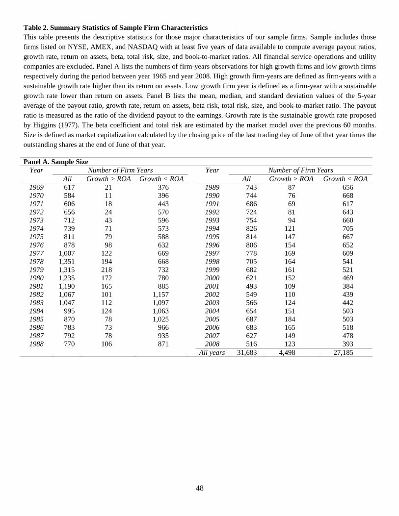
48

Table 2. Summary Statistics of Sample Firm Characteristics This table presents the descriptive statistics for those major characteristics of our sample firms. Sample includes those firms listed on NYSE, AMEX, and NASDAQ with at least five years of data available to compute average payout ratios, growth rate, return on assets, beta, total risk, size, and book-to-market ratios. All financial service operations and utility companies are excluded. Panel A lists the numbers of firm-years observations for high growth firms and low growth firms respectively during the period between year 1965 and year 2008. High growth firm-years are defined as firm-years with a sustainable growth rate higher than its return on assets. Low growth firm year is defined as a firm-year with a sustainable growth rate lower than return on assets. Panel B lists the mean, median, and standard deviation values of the 5-year average of the payout ratio, growth rate, return on assets, beta risk, total risk, size, and book-to-market ratio. The payout ratio is measured as the ratio of the dividend payout to the earnings. Growth rate is the sustainable growth rate proposed by Higgins (1977). The beta coefficient and total risk are estimated by the market model over the previous 60 months. Size is defined as market capitalization calculated by the closing price of the last trading day of June of that year times the outstanding shares at the end of June of that year. Panel A. Sample Size

Year Number of Firm Years Year Number of Firm Years All Growth > ROA Growth < ROA All Growth > ROA Growth < ROA

1969 617 21 376 1989 743 87 656 1970 584 11 396 1990 744 76 668 1971 606 18 443 1991 686 69 617 1972 656 24 570 1992 724 81 643 1973 712 43 596 1993 754 94 660 1974 739 71 573 1994 826 121 705 1975 811 79 588 1995 814 147 667 1976 878 98 632 1996 806 154 652 1977 1,007 122 669 1997 778 169 609 1978 1,351 194 668 1998 705 164 541 1979 1,315 218 732 1999 682 161 521 1980 1,235 172 780 2000 621 152 469 1981 1,190 165 885 2001 493 109 384 1982 1,067 101 1,157 2002 549 110 439 1983 1,047 112 1,097 2003 566 124 442 1984 995 124 1,063 2004 654 151 503 1985 870 78 1,025 2005 687 184 503 1986 783 73 966 2006 683 165 518 1987 792 78 935 2007 627 149 478 1988 770 106 871 2008 516 123 393

All years 31,683 4,498 27,185

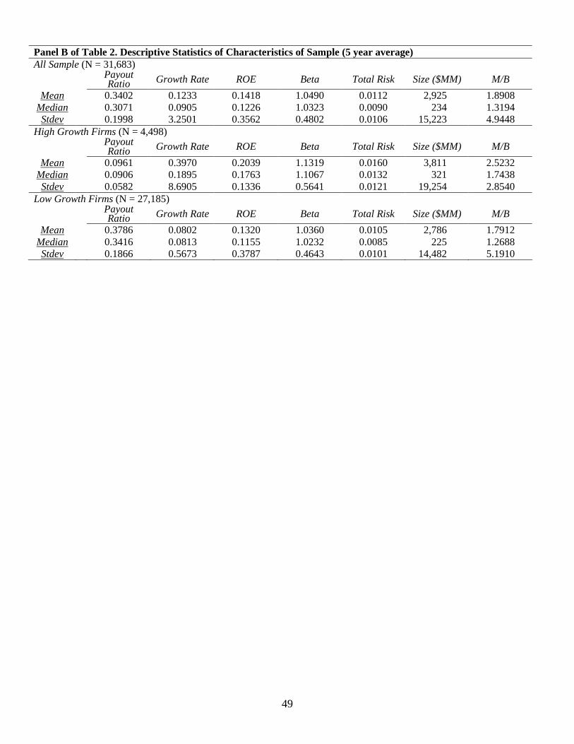
49

Panel B of Table 2. Descriptive Statistics of Characteristics of Sample (5 year average) All Sample (N = 31,683)

Payout Ratio Growth Rate ROE Beta Total Risk Size ($MM) M/B

Mean 0.3402 0.1233 0.1418 1.0490 0.0112 2,925 1.8908 Median 0.3071 0.0905 0.1226 1.0323 0.0090 234 1.3194 Stdev 0.1998 3.2501 0.3562 0.4802 0.0106 15,223 4.9448

High Growth Firms (N = 4,498)

Payout Ratio Growth Rate ROE Beta Total Risk Size ($MM) M/B

Mean 0.0961 0.3970 0.2039 1.1319 0.0160 3,811 2.5232 Median 0.0906 0.1895 0.1763 1.1067 0.0132 321 1.7438 Stdev 0.0582 8.6905 0.1336 0.5641 0.0121 19,254 2.8540

Low Growth Firms (N = 27,185)

Payout Ratio Growth Rate ROE Beta Total Risk Size ($MM) M/B

Mean 0.3786 0.0802 0.1320 1.0360 0.0105 2,786 1.7912 Median 0.3416 0.0813 0.1155 1.0232 0.0085 225 1.2688 Stdev 0.1866 0.5673 0.3787 0.4643 0.0101 14,482 5.1910

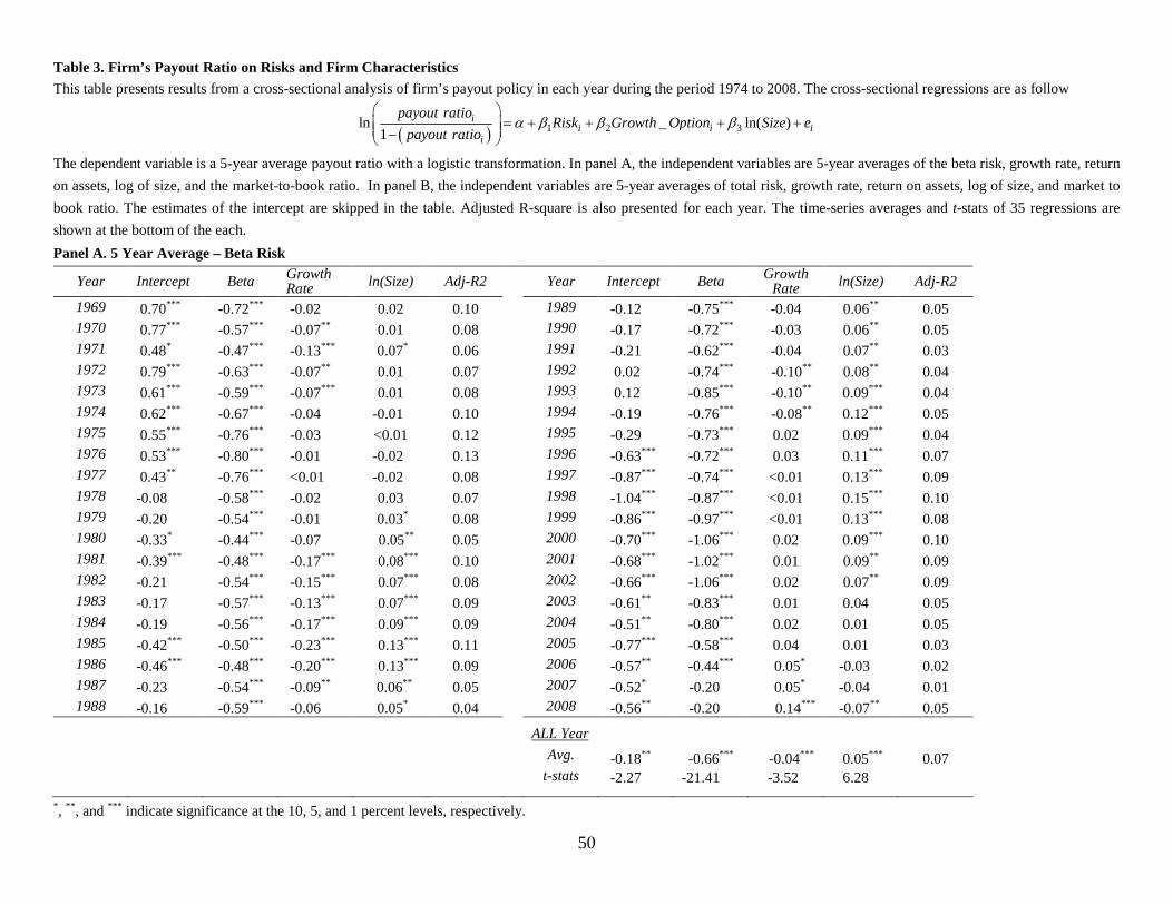
50

Table 3. Firm’s Payout Ratio on Risks and Firm Characteristics This table presents results from a cross-sectional analysis of firm’s payout policy in each year during the period 1974 to 2008. The cross-sectional regressions are as follow

( ) 1 2 3

ln _ ln( )1

ii i i

i

payout ratioRisk Growth Option Size e

payout ratioα β β β

= + + + + −

The dependent variable is a 5-year average payout ratio with a logistic transformation. In panel A, the independent variables are 5-year averages of the beta risk, growth rate, return

on assets, log of size, and the market-to-book ratio. In panel B, the independent variables are 5-year averages of total risk, growth rate, return on assets, log of size, and market to

book ratio. The estimates of the intercept are skipped in the table. Adjusted R-square is also presented for each year. The time-series averages and t-stats of 35 regressions are

shown at the bottom of the each.

Panel A. 5 Year Average – Beta Risk

Year Intercept Beta Growth Rate ln(Size) Adj-R2 Year Intercept Beta Growth

Rate ln(Size) Adj-R2

1969 0.70*** -0.72*** -0.02 0.02 0.10 1989 -0.12 -0.75*** -0.04 0.06** 0.05 1970 0.77*** -0.57*** -0.07** 0.01 0.08 1990 -0.17 -0.72*** -0.03 0.06** 0.05 1971 0.48* -0.47*** -0.13*** 0.07* 0.06 1991 -0.21 -0.62*** -0.04 0.07** 0.03 1972 0.79*** -0.63*** -0.07** 0.01 0.07 1992 0.02 -0.74*** -0.10** 0.08** 0.04 1973 0.61*** -0.59*** -0.07*** 0.01 0.08 1993 0.12 -0.85*** -0.10** 0.09*** 0.04 1974 0.62*** -0.67*** -0.04 -0.01 0.10 1994 -0.19 -0.76*** -0.08** 0.12*** 0.05 1975 0.55*** -0.76*** -0.03 <0.01 0.12 1995 -0.29 -0.73*** 0.02 0.09*** 0.04 1976 0.53*** -0.80*** -0.01 -0.02 0.13 1996 -0.63*** -0.72*** 0.03 0.11*** 0.07 1977 0.43** -0.76*** <0.01 -0.02 0.08 1997 -0.87*** -0.74*** <0.01 0.13*** 0.09 1978 -0.08 -0.58*** -0.02 0.03 0.07 1998 -1.04*** -0.87*** <0.01 0.15*** 0.10 1979 -0.20 -0.54*** -0.01 0.03* 0.08 1999 -0.86*** -0.97*** <0.01 0.13*** 0.08 1980 -0.33* -0.44*** -0.07 0.05** 0.05 2000 -0.70*** -1.06*** 0.02 0.09*** 0.10 1981 -0.39*** -0.48*** -0.17*** 0.08*** 0.10 2001 -0.68*** -1.02*** 0.01 0.09** 0.09 1982 -0.21 -0.54*** -0.15*** 0.07*** 0.08 2002 -0.66*** -1.06*** 0.02 0.07** 0.09 1983 -0.17 -0.57*** -0.13*** 0.07*** 0.09 2003 -0.61** -0.83*** 0.01 0.04 0.05 1984 -0.19 -0.56*** -0.17*** 0.09*** 0.09 2004 -0.51** -0.80*** 0.02 0.01 0.05 1985 -0.42*** -0.50*** -0.23*** 0.13*** 0.11 2005 -0.77*** -0.58*** 0.04 0.01 0.03 1986 -0.46*** -0.48*** -0.20*** 0.13*** 0.09 2006 -0.57** -0.44*** 0.05* -0.03 0.02 1987 -0.23 -0.54*** -0.09** 0.06** 0.05 2007 -0.52* -0.20 0.05* -0.04 0.01 1988 -0.16 -0.59*** -0.06 0.05* 0.04 2008 -0.56** -0.20 0.14*** -0.07** 0.05

ALL Year

Avg. -0.18** -0.66*** -0.04*** 0.05*** 0.07 t-stats -2.27 -21.41 -3.52 6.28

*, ** , and *** indicate significance at the 10, 5, and 1 percent levels, respectively.

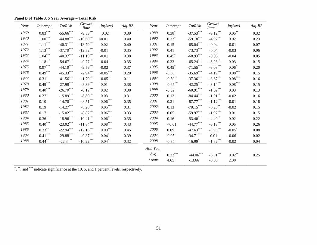
51

Panel B of Table 3. 5 Year Average – Total Risk

Year Intercept TotRisk Growth Rate ln(Size) Adj-R2 Year Intercept TotRisk Growth

Rate ln(Size) Adj-R2

1969 0.83*** -55.66*** -9.53*** 0.02 0.39 1989 0.38* -37.53*** -9.12*** 0.05** 0.32 1970 1.00*** -44.88*** -10.60*** <0.01 0.40 1990 0.33* -59.18*** -4.97*** 0.02 0.23 1971 1.11*** -40.31*** -13.79*** 0.02 0.40 1991 0.15 -65.04*** -0.04 -0.01 0.07 1972 1.13*** -37.70*** -12.32*** -0.01 0.35 1992 0.41 -73.73*** -0.04 -0.03 0.06 1973 1.04*** -40.37*** -11.19*** -0.01 0.38 1993 0.45* -68.93*** -0.06 -0.04 0.05 1974 1.18*** -54.67*** -9.77*** -0.04** 0.35 1994 0.33 -65.24*** -3.26*** 0.03 0.15 1975 0.97*** -44.10*** -9.56*** -0.03 0.37 1995 0.45* -71.55*** -6.08*** 0.06* 0.20 1976 0.49*** -45.33*** -2.94*** -0.05*** 0.20 1996 -0.30 -35.69*** -4.19*** 0.08*** 0.15 1977 0.31* -41.56*** -1.79*** -0.05** 0.11 1997 -0.50** -37.36*** -3.67*** 0.08*** 0.16 1978 0.49*** -27.98*** -8.39*** 0.01 0.38 1998 -0.65*** -42.25*** -3.14*** 0.08*** 0.15 1979 0.40*** -26.70*** -8.12*** 0.02 0.38 1999 -0.32 -60.91*** -1.62*** 0.03 0.13 1980 0.27* -15.89*** -8.80*** 0.03 0.31 2000 0.13 -84.44*** -1.01*** -0.02 0.16 1981 0.10 -14.70*** -8.51*** 0.06*** 0.35 2001 0.21 -87.77*** -1.12*** -0.01 0.18 1982 0.19 -14.27*** -8.20*** 0.05*** 0.31 2002 0.13 -79.15*** -0.25** -0.02 0.15 1983 0.17 -15.02*** -8.82*** 0.06*** 0.33 2003 0.05 -59.97*** -1.97*** 0.01 0.15 1984 0.36** -18.96*** -10.41*** 0.06*** 0.35 2004 0.16 -53.40*** -4.40*** 0.02 0.22 1985 0.40*** -23.02*** -11.84*** 0.08*** 0.43 2005 <0.01 -44.77*** -6.18*** 0.05 0.26 1986 0.33** -22.94*** -12.16*** 0.09*** 0.45 2006 0.09 -47.63*** -0.95*** -0.05* 0.08 1987 0.41*** -29.88*** -9.37*** 0.04* 0.39 2007 -0.05 -34.71*** 0.01 -0.06* 0.02 1988 0.44** -22.34** -10.22*** 0.04* 0.32 2008 -0.35 -16.99* -1.82*** -0.02 0.04

ALL Year

Avg. 0.32*** -44.06*** -6.01*** 0.02** 0.25 t-stats 4.65 -13.66 -8.88 2.30

*, ** , and *** indicate significance at the 10, 5, and 1 percent levels, respectively.

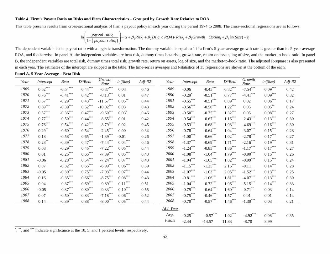
52

Table 4. Firm’s Payout Ratio on Risks and Firm Characteristics – Grouped by Growth Rate Relative to ROA

This table presents results from cross-sectional analysis of firm’s payout policy in each year during the period 1974 to 2008. The cross-sectional regressions are as follows:

( )( )1 2 3 4

ln _ ln( )

1 i

i i i ii

payout ratioRisk D g ROA Risk Growth Option Size e

payout ratioα β β β β

= + + < ⋅ + + + −

The dependent variable is the payout ratio with a logistic transformation. The dummy variable is equal to 1 if a firm’s 5-year average growth rate is greater than its 5-year average

ROA, and 0 otherwise. In panel A, the independent variables are beta risk, dummy times beta risk, growth rate, return on assets, log of size, and the market-to-book ratio. In panel

B, the independent variables are total risk, dummy times total risk, growth rate, return on assets, log of size, and the market-to-book ratio. The adjusted R-square is also presented

in each year. The estimates of the intercept are skipped in the table. The time-series averages and t-statistics of 35 regressions are shown at the bottom of the each.

Panel A. 5 Year Average – Beta Risk

Year Intercept Beta D*Beta Growth Rate ln(Size) Adj-R2 Year Intercept Beta D*Beta Growth

Rate ln(Size) Adj-R2

1969 0.62*** -0.54*** 0.44*** -6.87*** 0.03 0.46 1989 -0.06 -0.45*** 0.82*** -7.54*** 0.09*** 0.42 1970 0.76*** -0.41*** 0.42*** -8.13*** 0.01 0.47 1990 -0.29* -0.51*** 0.77*** -4.41*** 0.09*** 0.32 1971 0.67*** -0.29*** 0.43*** -11.67*** 0.05** 0.44 1991 -0.55*** -0.51*** 0.89*** 0.02 0.06*** 0.17 1972 0.69*** -0.39*** 0.52*** -10.02*** 0.03 0.43 1992 -0.56*** -0.50*** 1.22*** 0.05 0.05** 0.24 1973 0.57*** -0.36*** 0.47*** -9.60*** 0.03* 0.46 1993 -0.50** -0.75*** 1.32*** 0.05 0.08*** 0.27 1974 0.77*** -0.50*** 0.44*** -8.65*** 0.01 0.42 1994 -0.54*** -0.67*** 1.16*** -2.43*** 0.13*** 0.30 1975 0.76*** -0.54*** 0.42*** -8.79*** 0.02 0.45 1995 -0.53*** -0.68*** 1.08*** -4.69*** 0.16*** 0.30 1976 0.29** -0.60*** 0.54*** -2.45*** 0.00 0.34 1996 -0.78*** -0.64*** 1.04*** -3.07*** 0.15*** 0.28 1977 0.18 -0.58*** 0.65*** -1.39*** -0.01 0.26 1997 -1.00*** -0.66*** 1.02*** -2.78*** 0.17*** 0.27 1978 0.28** -0.39*** 0.47*** -7.44*** 0.04*** 0.46 1998 -1.37*** -0.69*** 1.71*** -2.16*** 0.19*** 0.31 1979 0.08 -0.29*** 0.45*** -7.22*** 0.05*** 0.44 1999 -1.24*** -0.85*** 1.86*** -1.17*** 0.17*** 0.27 1980 0.01 -0.25*** 0.65*** -7.39*** 0.05*** 0.43 2000 -1.08*** -1.04*** 1.79*** -0.90*** 0.15*** 0.26 1981 -0.06 -0.28*** 0.54*** -7.24*** 0.07*** 0.43 2001 -1.04*** -1.05*** 1.82*** -0.99*** 0.15*** 0.24 1982 0.07 -0.32*** 0.65*** -6.99*** 0.06*** 0.39 2002 -1.15*** -1.25*** 2.16*** -0.11 0.14*** 0.28 1983 -0.05 -0.30*** 0.75*** -7.03*** 0.07*** 0.44 2003 -1.07*** -1.03*** 2.05*** -1.52*** 0.13*** 0.25 1984 0.16 -0.35*** 0.66*** -8.75*** 0.08*** 0.43 2004 -0.81*** -1.06*** 1.81*** -4.07*** 0.13*** 0.30 1985 0.04 -0.37*** 0.69*** -9.89*** 0.11*** 0.51 2005 -1.04*** -0.72*** 1.96*** -5.15*** 0.14*** 0.33 1986 -0.05 -0.37*** 0.80*** -9.33*** 0.10*** 0.55 2006 -0.79*** -0.64*** 1.60*** -0.71** 0.03 0.14 1987 0.07 -0.50*** 0.83*** -7.18*** 0.06*** 0.52 2007 -0.75*** -0.46*** 1.57*** 0.01 0.01 0.14 1988 0.14 -0.39*** 0.88*** -8.00*** 0.05*** 0.44 2008 -0.70*** -0.57*** 1.46*** -1.30*** 0.03 0.21

ALL Year

Avg. -0.25** -0.57*** 1.02*** -4.92*** 0.08*** 0.35 t-stats -2.44 -14.57 11.83 -8.70 8.99

*, ** , and *** indicate significance at the 10, 5, and 1 percent levels, respectively.

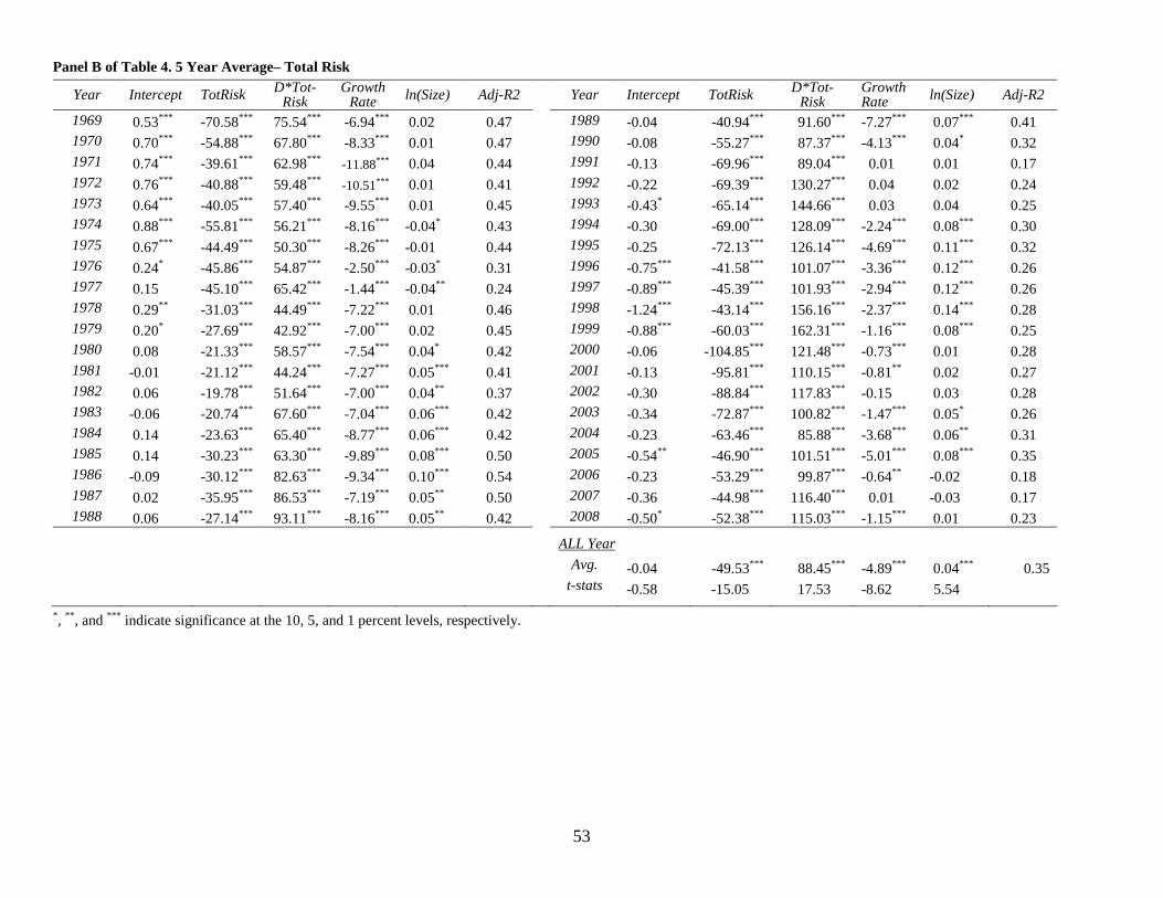
53

Panel B of Table 4. 5 Year Average– Total Risk

Year Intercept TotRisk D*Tot-Risk

Growth Rate ln(Size) Adj-R2 Year Intercept TotRisk D*Tot-

Risk Growth Rate ln(Size) Adj-R2

1969 0.53*** -70.58*** 75.54*** -6.94*** 0.02 0.47 1989 -0.04 -40.94*** 91.60*** -7.27*** 0.07*** 0.41 1970 0.70*** -54.88*** 67.80*** -8.33*** 0.01 0.47 1990 -0.08 -55.27*** 87.37*** -4.13*** 0.04* 0.32 1971 0.74*** -39.61*** 62.98*** -11.88*** 0.04 0.44 1991 -0.13 -69.96*** 89.04*** 0.01 0.01 0.17 1972 0.76*** -40.88*** 59.48*** -10.51*** 0.01 0.41 1992 -0.22 -69.39*** 130.27*** 0.04 0.02 0.24 1973 0.64*** -40.05*** 57.40*** -9.55*** 0.01 0.45 1993 -0.43* -65.14*** 144.66*** 0.03 0.04 0.25 1974 0.88*** -55.81*** 56.21*** -8.16*** -0.04* 0.43 1994 -0.30 -69.00*** 128.09*** -2.24*** 0.08*** 0.30 1975 0.67*** -44.49*** 50.30*** -8.26*** -0.01 0.44 1995 -0.25 -72.13*** 126.14*** -4.69*** 0.11*** 0.32 1976 0.24* -45.86*** 54.87*** -2.50*** -0.03* 0.31 1996 -0.75*** -41.58*** 101.07*** -3.36*** 0.12*** 0.26 1977 0.15 -45.10*** 65.42*** -1.44*** -0.04** 0.24 1997 -0.89*** -45.39*** 101.93*** -2.94*** 0.12*** 0.26 1978 0.29** -31.03*** 44.49*** -7.22*** 0.01 0.46 1998 -1.24*** -43.14*** 156.16*** -2.37*** 0.14*** 0.28 1979 0.20* -27.69*** 42.92*** -7.00*** 0.02 0.45 1999 -0.88*** -60.03*** 162.31*** -1.16*** 0.08*** 0.25 1980 0.08 -21.33*** 58.57*** -7.54*** 0.04* 0.42 2000 -0.06 -104.85*** 121.48*** -0.73*** 0.01 0.28 1981 -0.01 -21.12*** 44.24*** -7.27*** 0.05*** 0.41 2001 -0.13 -95.81*** 110.15*** -0.81** 0.02 0.27 1982 0.06 -19.78*** 51.64*** -7.00*** 0.04** 0.37 2002 -0.30 -88.84*** 117.83*** -0.15 0.03 0.28 1983 -0.06 -20.74*** 67.60*** -7.04*** 0.06*** 0.42 2003 -0.34 -72.87*** 100.82*** -1.47*** 0.05* 0.26 1984 0.14 -23.63*** 65.40*** -8.77*** 0.06*** 0.42 2004 -0.23 -63.46*** 85.88*** -3.68*** 0.06** 0.31 1985 0.14 -30.23*** 63.30*** -9.89*** 0.08*** 0.50 2005 -0.54** -46.90*** 101.51*** -5.01*** 0.08*** 0.35 1986 -0.09 -30.12*** 82.63*** -9.34*** 0.10*** 0.54 2006 -0.23 -53.29*** 99.87*** -0.64** -0.02 0.18 1987 0.02 -35.95*** 86.53*** -7.19*** 0.05** 0.50 2007 -0.36 -44.98*** 116.40*** 0.01 -0.03 0.17 1988 0.06 -27.14*** 93.11*** -8.16*** 0.05** 0.42 2008 -0.50* -52.38*** 115.03*** -1.15*** 0.01 0.23

ALL Year

Avg. -0.04 -49.53*** 88.45*** -4.89*** 0.04*** 0.35 t-stats -0.58 -15.05 17.53 -8.62 5.54

*, ** , and *** indicate significance at the 10, 5, and 1 percent levels, respectively.

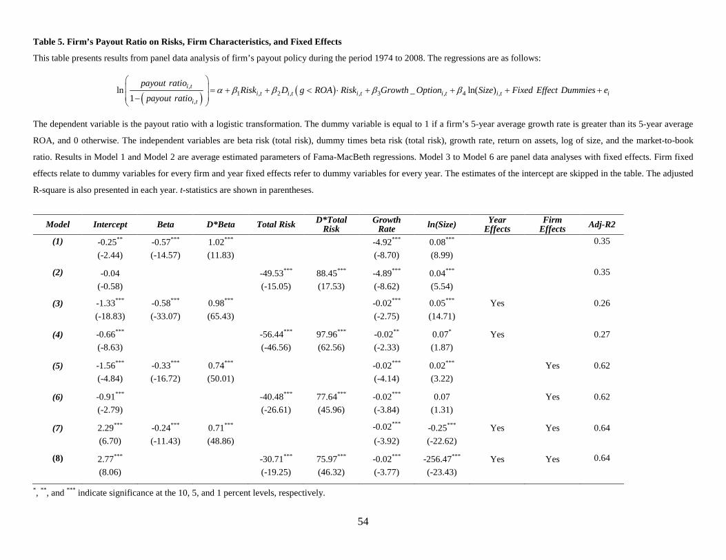
54

Table 5. Firm’s Payout Ratio on Risks, Firm Characteristics, and Fixed Effects

This table presents results from panel data analysis of firm’s payout policy during the period 1974 to 2008. The regressions are as follows:

( )( ),

1 , 2 , , 3 , 4 ,,

ln _ ln( )

1

i ti t i t i t i t i t i

i t

payout ratioRisk D g ROA Risk Growth Option Size Fixed Effect Dummies e

payout ratioα β β β β

= + + < ⋅ + + + + −

The dependent variable is the payout ratio with a logistic transformation. The dummy variable is equal to 1 if a firm’s 5-year average growth rate is greater than its 5-year average

ROA, and 0 otherwise. The independent variables are beta risk (total risk), dummy times beta risk (total risk), growth rate, return on assets, log of size, and the market-to-book

ratio. Results in Model 1 and Model 2 are average estimated parameters of Fama-MacBeth regressions. Model 3 to Model 6 are panel data analyses with fixed effects. Firm fixed

effects relate to dummy variables for every firm and year fixed effects refer to dummy variables for every year. The estimates of the intercept are skipped in the table. The adjusted

R-square is also presented in each year. t-statistics are shown in parentheses.

Model Intercept Beta D*Beta Total Risk D*Total Risk

Growth Rate ln(Size) Year

Effects Firm

Effects Adj-R2

(1) -0.25** -0.57*** 1.02*** -4.92*** 0.08*** 0.35

(-2.44) (-14.57) (11.83) (-8.70) (8.99)

(2) -0.04 -49.53*** 88.45*** -4.89*** 0.04*** 0.35

(-0.58) (-15.05) (17.53) (-8.62) (5.54)

(3) -1.33*** -0.58*** 0.98*** -0.02*** 0.05*** Yes 0.26

(-18.83) (-33.07) (65.43) (-2.75) (14.71)

(4) -0.66*** -56.44*** 97.96*** -0.02** 0.07* Yes 0.27

(-8.63) (-46.56) (62.56) (-2.33) (1.87)

(5) -1.56*** -0.33*** 0.74*** -0.02*** 0.02*** Yes 0.62

(-4.84) (-16.72) (50.01) (-4.14) (3.22)

(6) -0.91*** -40.48*** 77.64*** -0.02*** 0.07 Yes 0.62

(-2.79) (-26.61) (45.96) (-3.84) (1.31)

(7) 2.29*** -0.24*** 0.71*** -0.02*** -0.25*** Yes Yes 0.64

(6.70) (-11.43) (48.86) (-3.92) (-22.62)

(8) 2.77*** -30.71*** 75.97*** -0.02*** -256.47*** Yes Yes 0.64

(8.06) (-19.25) (46.32) (-3.77) (-23.43)

*, ** , and *** indicate significance at the 10, 5, and 1 percent levels, respectively.

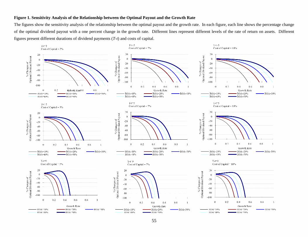
55

Figure 1. Sensitivity Analysis of the Relationship between the Optimal Payout and the Growth Rate

The figures show the sensitivity analysis of the relationship between the optimal payout and the growth rate. In each figure, each line shows the percentage change

of the optimal dividend payout with a one percent change in the growth rate. Different lines represent different levels of the rate of return on assets. Different

figures present different durations of dividend payments (T-t) and costs of capital.