Embed Size (px)
Citation preview

Optimal Need-Based Financial Aid
Mark Colas (University of Oregon)
Sebastian Findeisen (University of Konstanz)
Dominik Sachs (LMU Munich)
Discussion Paper No. 225December 18, 2019
Collaborative Research Center Transregio 190 | www.rationality-and-competition.de
Ludwig-Maximilians-Universität München | Humboldt-Universität zu Berlin
Spokesperson: Prof. Dr. Klaus M. Schmidt, University of Munich, 80539 Munich, Germany
+49 (89) 2180 3405 | [email protected]

Optimal Need-Based Financial Aid⇤
Mark Colas
University of Oregon
Sebastian Findeisen
University of Konstanz
Dominik Sachs
LMU Munich
December 15, 2019
Abstract
We study the optimal design of student financial aid as a function of parental income.We derive optimal financial aid formulas in a general model. For a simple model version,we derive mild conditions on primitives under which poorer students receive more aideven without distributional concerns. We quantitatively extend this result to an empiri-cal model of selection into college for the United States that comprises multidimensionalheterogeneity, endogenous parental transfers, dropout, labor supply in college, and uncer-tain returns. Optimal financial aid is strongly declining in parental income even withoutdistributional concerns. Equity and efficiency go hand in hand.
JEL-classification: H21, H23, I22, I24, I28
Keywords: Financial Aid, College Subsidies, Optimal Taxation, Inequality
⇤Contact: [email protected], [email protected], [email protected]. An ear-lier version of this paper was circulated under the title “Designing Efficient College and Tax Policies”. We thankJames J. Heckman, the editor, as well as four anonymous referees. We also thank Rüdiger Bachmann, FelixBierbrauer, Richard Blundell, Christian Bredemeier, Friedrich Breyer, David Card, Pedro Carneiro, JonathanM.V. Davis, Juan Dolado, Alexander Gelber, Marcel Gerard, Emanuel Hansen, Jonathan Heathcote, NathanielHendren, Bas Jacobs, Leo Kaas, Marek Kapicka, Kory Kroft, Paul Klein, Tim Lee, Lance Lochner, NormannLorenz, Thorsten Louis, Alex Ludwig, Marti Mestieri, Nicola Pavoni, Michael Peters, Emmanuel Saez, AlehTsyvinski, Gianluca Violante, Matthew Weinzierl, Nicolas Werquin, and seminar participants at Berkeley,Bocconi, Bonn (MPI & MEE), CEMFI, Dortmund, EIEF, EUI, Frankfurt, IFS/UCL, Lausanne, Louvain(CORE), Minneapolis FED, Notre Dame, NYU, Queen’s, Salzburg, St. Gallen, Tinbergen, Toronto, Toulouse,Uppsala, Warwick, and Yale, as well as conference participants at CEPR Public Meeting 16, CEPR Conferenceon Financing Human Capital 18, CESifo Public Sector Economics, IIPF, NBER SI Macro Public Finance,NORMAC, SEEK, and the Taxation Theory Conference. We thank Mehmet Ayaz for careful proofreading.Dominik Sachs’ research was partly funded by a post-doc fellowship of the Fritz-Thyssen Foundation and theCologne Graduate School in Management, Economics and Social Sciences. Financial support by DeutscheForschungsgemeinschaft through CRC TRR 190 (project number 280092119) is gratefully acknowledged
1 Introduction
In all OECD countries, college students benefit from financial support (OECD, 2014). More-over, with the goal of guaranteeing equality of opportunity, financial aid is typically need-based and targeted specifically to students with low parental income. In the United States,the largest need-based program is the Pell Grant. Federal spending on this program exceeded$30 billion in 2015 and has grown by over 80% during the last 10 years (College Board, 2015).One justification for student financial aid in the policy debate is that the social returns tocollege exceed the private returns because the government receives a share of the financialreturns through higher tax revenue (Carroll and Erkut, 2009; Baum et al., 2013). This lowersthe effective fiscal costs (i.e., net of tax revenue increases) of student financial aid.1
In this paper, we study the optimal design of financial aid and show that consideringdynamic scoring aspects is crucial to assessing the desirability of need-based programs suchas the Pell Grant. The reduction in the effective fiscal costs of student financial aid due todynamic fiscal effects varies along the parental income distribution. We show that effectivefiscal costs are increasing in parental income and are therefore lowest for those children thatare targeted by the Pell Grant. The policy implication is that need-based financial aid isdesirable not only because it promotes intergenerational mobility and equality of opportunity.Need-based financial aid is also desirable from an efficiency point of view because subsidizingthe college education of children from weak parental backgrounds is cheaper for society thansubsidizing students from "average" parental backgrounds. The usual equity-efficiency trade-off does not apply for need-based financial aid.
To arrive there, we start with a general model without imposing restrictions on the under-lying heterogeneity in the population. Further, besides enrollment, labor supply and savingsdecisions, we consider dropout, labor supply during college and endogenous parental trans-fers. We derive a simple optimality condition for financial aid that transparently highlightsthe key trade-offs. At a given level of parental income, optimal financial aid decreases in theshare of inframarginal students, which captures the marginal costs. These costs are scaleddown by the marginal social welfare weights attached to these students. Optimal financial aidincreases in the share of marginal students2 and the fiscal externality per marginal student,which jointly capture the marginal benefits of the subsidy. The fiscal externality is the changein lifetime fiscal contributions causal to college attendance.3 For the optimality condition, the
1The Congressional Budget Office (CBO), following a request by the Senate Committee on the Budget,recently documented the growth in the fiscal costs of Pell Grant spending (Alsalam, 2013). Dynamic scoringaspects are neglected in this report: the positive fiscal effects through higher tax revenue in the future arenot taken into account. Generally, the CBO does consider issues of dynamic scoring: https://www.cbo.gov/publication/50919.
2Those students that are at the margin of attending college with respect to financial aid.3On top of that, financial aid is also increasing in the completion elasticity with respect to financial aid
and the fiscal externality due to completing college instead of dropping out. This channel, however, turns outto be quantiatively of minor importance.
1
specific reason why marginal students change their behavior due to a change in subsidies (e.g.,borrowing constraints or preferences) is not important.
Elasticities linking changes in enrollment behavior to changes in financial aid have beenestimated in the literature (e.g., by Dynarski (2003) and Castleman and Long (2016)). Thesepapers provide guidance about the average value of this policy elasticity or about its value ata particular parental income level. However, knowledge about how this elasticity varies alongthe parental income distribution is missing. Knowledge of those parameters for students fromdifferent parental income groups, however, is necessary to analyze the welfare effects of need-based financial aid. Further, these elasticities are not deep parameters but do change as policychanges. The main approach of this paper is therefore a structural model of selection intocollege that allows us to compute this policy elasticity along the parental income distributionand for alternative policies.
As a first step, however, before studying this empirical model, we consider a simple theo-retical setting. We reduce the complexity of the problem by focusing on two dimensions ofheterogeneity: (i) parental transfers and (ii) returns to college. Further, we simplify the modelby making the problem static, shutting down risk, labor supply during college and dropout.We first show that financial aid is decreasing in parental income even in the absence of dis-tributional concerns if the distribution of returns is log concave (which implies a decreasinghazard rate)4 and if returns and parental income are independently distributed. We thenshow that these analytical results extend to the empirically more plausible case of a positiveassociation between parental income and child ability.5
We then move to our structural life-cycle model, where we account for earnings risk,dropout, labor supply during college and, importantly, we account for crowd-out of parentaltransfers by explicitly modeling parental decisions to save, consume and provide transfersto their children. Another additional crucial ingredient of the model is heterogeneity in thepsychic costs of education because monetary returns can only account for a small part of theobserved college attendance patterns (Heckman et al., 2006). Using data from the NationalLongitudinal Survey of Youth 1979 and 1997, we estimate the parameters of our model viamaximum likelihood and provide a detailed discussion of how variation in the data helps usto identify the crucial parameters.
We find that optimal financial aid policies are strongly progressive. In our preferred specifi-cation, the level of financial aid drops by 48% moving from the 25th percentile of the parentalincome distribution to the 75th percentile. The strong progressivity result does not rely onthe Utilitarian welfare criterion. We show that a social planner that sets equal social wel-fare weights on all students or is only interested in maximizing tax revenues would choose
4The hazard rate pins down the ratio of marginal over inframarginal students which is also key in thissimplified model.
5We obtain this clear analytical result if the ability distribution of high parental income children dominatesthe distribution of low parental income children in the hazard rate order. For a Pareto distribution, e.g., theproperty of hazard rate dominance always holds in case of first-order stochastic dominance.
2

an almost equally progressive financial aid schedule. Second, our estimates suggest that tar-geted increases in financial aid for students below the 59th percentile of the parental incomedistribution, are self-financing by increases in future tax revenue; this implies that targetedfinancial aid expansions could be free-lunch policies. Both results point out that financial aidpolicies for students are a rare case in which there is no equity-efficiency trade-off.
In a last step, we provide several extensions and robustness checks. We show that our pro-gressivity result also holds if we (i) remove borrowing constraints, (ii) choose the merit-baseddimension of financial aid optimally, (iii) allow the government to set an optimal Mirrleesianincome tax schedule, (iv) model early educational investments and thereby endogenize abilityand (v) if the relative wage for college educated labor is determined in general equilibrium.
Our paper contributes to the existing literature in several ways. Stantcheva (2017) char-acterizes optimal human capital policies in a very general dynamic model with continuouseducation choices. The main differences with our approach are twofold. First, theoretically,we study a model with discrete education choices as we find this a natural way to study finan-cial aid policies. As we show, the optimality conditions are quite distinct from the continuouscase and different elasticities are required to characterize the optimum. Second, the extensivemargin education decision allows us to incorporate a large degree of heterogeneity withoutmaking the optimal policy problem intractable. This allows for a modeling approach that isclose to the empirical, structural literature.
Bovenberg and Jacobs (2005) consider a static model with a continuous education choiceand derive a “siamese twins” result: they find that the optimal marginal education subsidyshould be as high as the optimal marginal income tax rate, thereby fully offsetting the dis-tortions from the income tax on the human capital margin.6 Lawson (2017) uses an elasticityapproach to characterize optimal uniform tuition subsidies for all college students.7 Jacobs andThuemmel (2018) study the role of skill-biased technical change for optimal college subsidiesand income taxation. We contribute to this line of research by developing a new framework toanalyze how education policies should depend on parents’ resources and also trade off merit-based concerns. Our theoretical characterization of optimal financial aid (and tax policies)allows for a large amount of heterogeneity, and we tightly connect our theory directly to thedata by estimating the relevant parameters ourselves. Finally, the paper is also related tomany empirical papers, from which we take the evidence to gauge the performance of theestimated model. These papers are mentioned in Section 4.
6Bohacek and Kapicka (2008) derive a similar result as in a dynamic deterministic environment. Findeisenand Sachs (2016), focus on history-dependent policies and show how history-dependent labor wedges can beimplemented with an income-contingent college loan system. Koeniger and Prat (2017) study optimal history-dependent human capital policies in a dynastic economy where education policies also depend on parentalbackground. Stantcheva (2015) derives education and tax policies in a dynastic model with multi-dimensionalheterogeneity, characterizing the relationship between education and bequest policies.
7Our work is also complementary to Abbott et al. (2018) and Krueger and Ludwig (2013, 2016), who studyeducation policies computationally in very rich overlapping-generations models.
3

We progress as follows. In Section 2 we develop the general model and characterize theoptimal policies in terms of reduced-form objects. In Section 3 we consider a simplified versionof the model, which allows us to transparently study mild conditions on primitives underwhich financial aid is optimally decreasing in parental income. In Section 4 we specify ourquantitative model as a special case of the general model presented in Section 2 and presentour estimation approach. Section 5 presents optimal financial aid policies, and Section 6decomposes the forces which lead to an optimal financial aid schedule. In Section 7 we discussfurther robustness issues. Section 8 concludes.
2 Optimal Financial Aid Policies
In this section we characterize optimal (need-based) financial aid policies for college students.Our approach is to work with a general model and characterize the optimal financial aid interms of reduced-form objects. This formula is general on the one hand and economicallyintuitive on the other hand. It clearly highlights the role of the fiscal externality as a reasonfor why education is subsidized (Bovenberg and Jacobs 2005). The fiscal externality arisesthrough the tax-transfer system: if college increases human capital and therefore earnings,college education implies a fiscal externality since the individual will pay more taxes. Hence,if the government imposed lump sum taxes that were independent of earnings, there would beno fiscal externality. In Section 4, we explore the quantitative implications of this optimalitycondition in a fully specified structural empirical model, which is a special case of the modelanalyzed in Section 2. As an intermediate step, we theoretically explore a simplified frameworkin Section 3, for which we can derive conditions on primitives that imply that optimal financialaid is indeed need-based, i.e., that financial aid is decreasing in parental income, even in theabsence of distributional concerns.
2.1 Individual Problem
Individuals start life in year t = 0 as high school graduates and are characterized by a vectorof characteristics X 2 � and (permanent) parental income I 2 R+. Life lasts T periods andindividuals face the following decisions. At the beginning of the model, they face a binarychoice: enrolling in college or not. If individuals decide against enrollment, they directly enterthe labor market and make labor-leisure decisions every period. If individuals decide to enrollin college, they also make a labor-leisure decision during college and, at the beginning of theyear, decide to drop out or continue. After graduating or dropping out, individuals enter thelabor market.
We start by considering labor market decisions of individuals that either are out of collegeor have chosen to forgo college altogether. This is a standard labor-leisure-savings problem
4

with incomplete markets. Let VW
t(·) denote the value function of an individual in the labor
market in year t. Then the recursive problem is given by
VW
t(X, I, e, at, wt) =max
ct,`t
U(ct, `t) + �E⇥V
W
t+1(X, I, e, at+t, wt+1)|wt
⇤
subject to the budget constraint
ct + at+1 = `twt � T (`twt) + at(1 + r) + trt(X, I, e, wt).
The state variables are the initial characteristics (X, I), the education level e 2 {H,D,G}(high school graduate, college dropout, college graduate), assets at, and the current wagewt. The variables (X, I, e) are state variables because they may affect parental transferstrt(X, I, e, wt) and because they may affect the evolution of future wages. The dependenceon the education decision then captures the returns to education. The function T capturesthe tax-transfer system. Finally, we assume that the utility function is such that there areno income effects on labor supply. Given those value functions, we now turn to the valuefunctions of the different education decisions. The value of not enrolling in college (i.e.,choosing education level H) is simply given by
VH(X, I) =E
⇥V
W
1 (X, I, e = H, a1 = 0, w1)⇤.
Regarding the realization of uncertainty, the timing is such that individuals directly enter thelabor market in period one and draw their first wage w1, which is hence only known after theeducation decision has been made. Next, we turn to the decisions during college. Besides thequestion of how much to work and consume while in college, individuals also make the binarydecision of dropping out or staying enrolled.
The value function of a college student at age t is given by
VE
t(X, I, at, "t) = max[V ND
t(X, I, at, "t), V
D
t(X, I, at, "t)]
where VD(·) is the value function associated with dropping out, V
ND
t(·) denotes the value
function of staying enrolled (not dropping out), and "t is a vector of preference shocks. Agentswho drop out of college enter the labor force and may also pay a psychic cost associated withdropping out. The value of dropping out is therefore given by:
VD
t(X, I, at) =E
⇥V
W
t(X, I, e = D, at, wt)
⇤� d ("t)
where d ("t) represents the psychic cost of dropping out.The value function for staying enrolled is a bit more complex and given by:
5
VND
t(X, I, at, "t) = max
ct,`E
t
[UE�ct, `
E
t;X, "t
�+
���
1� PrGrad
t(X)
�⇥ E
⇥V
E
t+1 (X, I, at+1, "t+1)⇤+ Pr
Grad
t(X)⇥ E
⇥V
W
t+1 (X, I, e = G, at+1, wt+1)⇤
subject to
ct = `E
t! + at (1 + r (at, I))� at+1 � F(X) + G (X, I) + tr
E
t(X, I,G(X, I))
andat+1 � a
E
t+1.
w is the wage that students earn if they work during college and F(X) is tuition. Tuition mightvary by X because of regional differences in college tuition, for example. We denote work incollege by `
E
t.8 The term G(X, I) is the amount of financial aid a student with characteristics
X and parental income I receives, and trE
t(X, I,G(X, I)) captures parental transfers in year
t for children that are enrolled in college. They are endogenous with respect to the level offinancial aid to account for the potential crowding out of parental transfers through financialaid. Pr
Grad
t(X) is a stochastic graduation probability which can depend on the vector X.
We allow the interest rate for college enrollees to vary by the agent’s asset position (positiveor negative) and by the agent’s parental income. We denote flow utility while enrolled incollege by U
E(ct, `Et ;X, "t). Importantly, this flow utility may include the psychic costs andnonpecuniary benefits of college attendance, in addition to flow utility from consumption andlabor supply. These psychic costs have been found to be important in explaining college en-rollment patterns.9 The flow utility in college can depend directly on personal characteristics,X, allowing these psychic costs of college to vary with the individual’s characteristics. Notethat the vector of personal characteristics, X, may also include idiosyncratic preferences forenrolling in college.
Finally we denote the value of enrolling into college in the first place as
VE(X, I) = E
⇥V
E
1 (X, I, a1 = 0, "1)⇤+ �(X),
where �(X) is a function that gives any additional nonpecunairy benefits of enrolling in collegefor agents with characteristics X. An individual enrolls in college if V E(X, I) � V
H(X, I).Denote by P
D
t(X, I,G(X, I)) the share of individuals of type (X, I) that drop out in period
t. Importantly the model captures the idea that the dropout decision is endogenous with8We assume these earnings are not taxed. In the data, the average earnings of students who work in
college are so low that they do not have to pay positive income taxes; in addition, the vast majority of collegestudents does not qualify for welfare/transfer programs.
9See Cunha et al. (2005), Heckman et al. (2006) or Heckman and Navarro (2007).
6
respect to financial aid. Further, denote by PE
t(X, I,G(X, I)) =
Qt
s=1(1�PD
s(X, I,G(X, I))⇥
Qt�1s=1
�1� Pr
Grad
s(X)
�the proportion of all initially enrolled students that are enrolled in
period t. Finally, we denote the proportion of initially enrolled students that successfullycomplete college by P
C(X, I,G(X, I)) =Pt
maxg
t=1 PE
t(X, I,G(X, I))Pr
Grad
t(X). We move to the
policy analysis and for the remainder of the section make three simplifying assumption for thepurpose of simpler notation. We assume that individuals can only drop out after two yearsin college such that P
D
t(X, I,G(X, I)) = 0 if t 6= 3 and cannot graduate before year t = 3,
i.e. PrGrad
t(X) = 0 for t = 1, 2.10 Finally, we assume that financial aid only depends only on
parental income, and not on other characteristics, X. We therefore write financial aid as G(I)for the remainder of this section.11
2.2 Fiscal Contributions
We now define the expected net fiscal contributions for different types (X, I) and differenteducation levels as these will be key ingredients for the policy analysis. We start with the netpresent value (NPV) in net tax revenues of high school graduates of type (X, I):
NT H
NPV(X, I) =
TX
t=1
✓1
1 + r
◆t�1
E (T (yt)|X, I,H) ,
where yt = wt`t is total earnings in year t.The fiscal contribution of a dropout is given by their net present value of tax payments
minus grants received:
NT D
NPV(X, I) =
TX
t=3
✓1
1 + r
◆t�1
E (T (yt)|X, I,D)� G(I)2X
t=1
✓1
1 + r
◆t�1
.
Finally, we turn to students that do not dropout but graduate. The average fiscal contri-bution of graduates of type (X, I) is given by:
NT G
NPV(X, I) =
1Ptmax
g
g=3 PEg(X, I,G(I))PrGrad
g(X)
tmaxgX
g=3
PE
g(X, I,G(I))Pr
Grad
g(X)
"TX
t=g+1
✓1
1 + r
◆t�1
E (T (yt)|X, I,G)� G(I)gX
t=1
✓1
1 + r
◆t�1#
10We provide the optimal policy formulas without these simplifying assumptions in Appendix A.2. Theintuition of these formulas are the same but the notation is considerably more cumbersome.
11We allow for other characteristics to enter the financial aid formula in the quantitative version of themodel in Section 4. We show that our main result also extends to the case in which the merit-based elementsare chosen optimally in Appendix C.10.
7

where tmax
gis the latest possible graduation date. Finally, we define the expected fiscal con-
tribution of an individual that decides to enroll:
NT E
NPV(X, I) = P
C(X, I,G(I))⇥NT G
NPV(X, I) + (1� P
C(X, I,G(I)))⇥NT D
NPV(X, I).
Before we derive optimal education subsidies, we ease the upcoming notation a little bit.Let a type (X, I) be labeled by j and define the enrollment share for income level I:
E(I) =
Z
�
1VE
j�V
H
j
h(X|I)dX,
where 1VE
j�V
H
j
is an indicator function capturing the education choice for each type j = (X, I).Next, we define the completion rate by
C(I) =
R�1V
E
j�V
H
j
PC(X, I,G(I))h(X|I)dX
E(I),
which captures the share of enrolled students of parental income level I that actually graduate.We assume that these shares, as well as the probabilities of dropping out, PD
t(X, I,G(I)), are
differentiable in the level of financial aid.
2.3 Government Problem and Optimal Policies
We now characterize the optimal financial aid schedule G(I). We denote by F (I) the un-conditional parental income CDF, by K(X, I) the joint CDF and by H(X|I) the conditionalone; the densities are f(I), k(X, I), and h(X|I), respectively. The government assigns Paretoweights k(X, I) = f(I)h(X|I), which are normalized to integrate up to one.
Importantly, we assume that the government takes the tax-transfer system T (·) as givenand consider the optimal budget-neutral reform of G(I). Whereas the tax-transfer system isnot changed if financial aid is reformed, a change in the financial aid schedule changes the sizeand the composition of the set of individuals that go to college. This implies a change in taxrevenue and transfer spending that directly feeds back into the available resource for financialaid.12 Taking the tax-transfer system as given, the problem of the government is
maxG(I)
Z
R+
Z
�
max{V E(X, I), V H(X, I)}k(X, I)dXdI (1)
subject to the net present value government budget constraint:12We consider this as the more policy-relevant exercise than considering the joint optimal choice of T (·) and
G(I). Nevertheless, to complete the picture, in Appendix C.9, we consider the joint optimal design of financialaid G(I) and the tax-transfer system T (·). Further, we also explore jointly optimal merit and need-basedfinancial aid in Appendix C.10.
8
Z
R+
Z
�
NT H
NPV(X, I)1V
E
j<V
H
j
k(X, I)dXdI
+
Z
R+
Z
�
NT G
NPV(X, I)1V
E
j�V
H
j
PC(X, I,G(I))k(X, I)dXdI
+
Z
R+
Z
�
NT D
NPV(X, I)1V
E
j�V
H
j
�1� P
C(X, I,G(I))�k(X, I)dXdI � F , (2)
The term F captures exogenous revenue requirements (e.g. spending on public goods) andexogenous revenue sources (e.g. tax revenue from older cohorts). Hence, F < 0 could capturethat the cohort for which we are reforming the financial aid schedule is effectively subsidizedfrom other cohorts. Now we consider a marginal increase in G(I). As we show in Appendix A.1,it has the following impact on welfare:
@E(I)
@G(I) ⇥�T E(I)| {z }Enrollment Effect
+@C(I)
@G(I)
�����E(I)
⇥ E(I)⇥�T C(I)
| {z }Completion Effect
� E(I)�1�W
E(I)�
| {z }Mechanical Effect
= 0. (3)
The first two terms of (3) capture behavioral effects (i.e., changes in welfare that are due toindividuals changing their behavior). The third term captures the mechanical welfare effect(i.e. the welfare effect that would occur for fixed behavior). We start with the latter.
The mechanical effect captures the direct welfare impact of the grant increase to infra-marginal students. The more students are inframarginal in their decision to go to college andthe more of them do not drop out, the higher are the immediate costs of the grant increase.The term E(I) is the total discounted years of college attendance of income group I and isdefined as
E(I) =
Z
�
1VE
j�V
H
j
0
@tmaxgX
t=1
✓1
1 + r
◆t�1
PE
t(X, I,G(I))
1
Ah(X|I)dX.
This captures the direct marginal fiscal costs of the grant increase. Since the utility of thesestudents is valued by the government, the costs have to be scaled down by a social marginalwelfare weight (Saez and Stantcheva, 2016). We denote average social marginal welfare weightof inframarginal students with parental income I by W
E(I). Formally it is given by
WE(I) =
R�1V
E
j�V
H
j
EhPt
maxg
t=1 �t�1
UE
c(·)⇣1 + @tr
E
t(·)
@G(I)
⌘Qt
s=1(1V NDs �V D
s)Q
t�1s=1
�1� Pr
Grad
s(X)
�ih(X|I)dX
⇢f(I)
f(I)E(I)
,
9
where ⇢ is the marginal value of public funds, UE
cis the marginal utility of consumption,
and 1V NDs �V D
sis an indicator for an individual choosing not to drop out of college in year
s. Thus, WE(I) is a money-metric (appropriately weighted) average marginal social welfareweight. One difference from the standard concept applies here, however. One has to correctfor the implied reduction in parental transfers that accompanies an increase in resourcesfor college students. For each marginal dollar of additional grants, students only have achange in consumption that is given by
⇣1 + @tr
E
t(X,I,G(I))@G(I)
⌘. Ceteris paribus, the stronger the
crowding out of transfers, the lower are these welfare weights since fewer of the additionalgrants effectively reach students.13
We now turn to the behavioral welfare effects in the first line of (3). The first term capturesthe change in tax revenues due to an increase in enrollment and @E(I)
@G(I) captures the additionalenrollees. Since these individuals are marginal in their enrollment decision, this change in theirdecision has no first-order effect on their utility. Therefore, we only have to track the effecton welfare through the effect on public funds. The term �T E(I) captures the the averageincrease in the NPV of net tax revenues for these marginal enrollees. Formally, it is given by
�T E(I) =
R�1Hj!Ej
�T E(X, I) h(X|I)dXR�1Hj!Ej
h(X|I)dX, (4)
where 1Hj!Ejtakes the value one if an individual of type j is marginal in her college en-
rollment decision with respect to a small increase in financial aid. By definition we haveR�1Hj!Ej
h(X|I)dX = @E(I)@G(I) . �T E(X, I) is the (expected) fiscal externality of an individual
of type (X, I): �T E(X, I) = NT E
NPV(X, I)�NT H
NPV(X, I).
There is a second behavioral effect due to endogenous college dropout. This second termin (3) captures the increase in tax revenue due to an increase in the completion rate of theinframarginal enrollees. The term @C(I)
@G(I)
���E(I)
is the partial derivative of completion w.r.t.
financial aid, holding E(I) constant. Therefore, the term @C(I)@G(I)
���E(I)
⇥ E(I) captures theamount of inframarginal enrollees who did not graduate in the absence of the grant increasebut graduate now. Again, the envelope theorem applies and the change in their behavior hasno first-order effect on their utility. However, there is a welfare effect through the changein public funds. �T C(I) captures the implied change in net fiscal contributions through theincreased completion rate:
�T C(I) =
R��T C(X, I)@P
C(X,I,G(I))@G(I) h(X|I)dX
R�
@PC(X,I,G(I))@G(I) h(X|I)dX
,
13Note that we are not accounting for parents’ utilities here. Doing so would basically imply an increase inthe social welfare weights as not only the children but also the altruistic parents are benefiting from the grants.The change in parental transfers would have no impact on parent’s utility due to the envelope theorem.
10

where �T C(X, I) = NT G
NPV(X, I) � NT D
NPV(X, I). Finally, note that formula (3) is inde-
pendent of the adjustment in labor supply during college as a response to the grant increase.This is an implication of the envelope theorem.
Formula (3) expresses the optimal policy as a function of reduced-form elasticities andprovides intuition for the main trade-offs underlying the design of financial aid.14 It is validwithout taking a stand on the functioning of credit markets for students, the riskiness ofeducation decisions, or the exact modeling of how parental transfers are influenced by parentalincome and how they respond to changes in financial aid. Those factors, of course, influencethe values of the reduced-form elasticities. For example, a tightening of borrowing constraintsshould increase the sensitivity of enrollment especially for low-income students.
However, note that all terms in the optimal financial aid formula are endogenous withrespect to policies. Even if we know the empirical values for current policies, this is notenough to calculate optimal policies. For this purpose, a fully specified model is necessary.In the next Section 3, we consider a simplified model, for which we can derive closed-formsolutions.15
3 Is Optimal Financial Aid Progressive? A Simple Model
Simplified Environment. We assume that preferences are linear in consumption and thatlabor incomes are taxed linearly at rate ⌧ , which is larger than 0 and smaller than one.We consider a static problem. If individuals do not go to college, they earn income yH . Ifthey go to college, they pay tuition F and earn yH(1 + ✓). Individuals are heterogeneous inability/returns to college, ✓, and each ✓ > 0. There is no uncertainty. Further, individualsare heterogeneous in parental income I. If individuals go to college, they receive a parentaltransfer tr(I) with tr
0(I) > 0 and financial aid G(I).
Individual Problem. If an individual decides against college, utility is given by UH =
(1� ⌧)yH . If an individual goes to college, utility is given by UC(✓, I) = (1� ⌧) yH (1 + ✓)�
(F � G(I)� tr(I)). For each income level I, we can define the ability of the marginal collegegraduate ✓(I), implicitly given by U
H = UC(✓(I), I). All types (✓, I) with ✓ � (<)✓(I) (do
not) attend college. Note that higher parental income here simply has the role of lowering thecosts of college. This implies that high-parental-income children are more likely to select intocollege. This channel is reinforced if there is a positive association between I and ✓.
Government Problem and Optimal Financial Aid for a Given I. The governmentuses non-negative Pareto weights over the types as in the general model from the last section.
14Sometimes such formulas are labeled as sufficient statistics formulas. See Kleven (2018) for a discussionon the terminology in the literature.
15We are very grateful to one of our referees for many detailed suggestions how to clarify the intuitionbehind the results in Section 3.
11
Consistent with the notation from last section, F (I) is the parental income distribution andH(✓|I) the conditional distribution of ability. Appendix A.3 shows that the following versionof equation (3) holds:
h(✓(I)|I)yH(1� ⌧)| {z }
@E(I)@G(I)
⇥⇣⌧yh✓(I)� G(I)
⌘
| {z }�T E(I)
�⇣1�H(✓(I)|I)
⌘
| {z }E(I)
(1�WE(I)) = 0.
First note that there is no completion effect since we abstract from dropout. Second, thefiscal externality takes a simple form. Third the ratio of marginal over inframarginal studentsis determined by the hazard rate of the conditional skill distribution. Rewriting leads to arather tractable expression for optimal financial aid G(I).
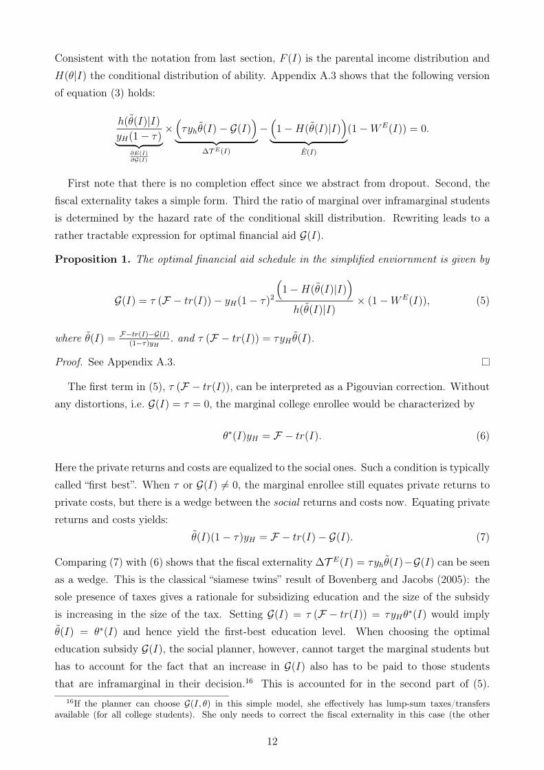
Proposition 1. The optimal financial aid schedule in the simplified enviornment is given by
G(I) = ⌧ (F � tr(I))� yH(1� ⌧)2
⇣1�H(✓(I)|I)
⌘
h(✓(I)|I)⇥ (1�W
E(I)), (5)
where ✓(I) = F�tr(I)�G(I)(1�⌧)yH
. and ⌧ (F � tr(I)) = ⌧yH ✓(I).
Proof. See Appendix A.3.
The first term in (5), ⌧ (F � tr(I)), can be interpreted as a Pigouvian correction. Withoutany distortions, i.e. G(I) = ⌧ = 0, the marginal college enrollee would be characterized by
✓⇤(I)yH = F � tr(I). (6)
Here the private returns and costs are equalized to the social ones. Such a condition is typicallycalled “first best”. When ⌧ or G(I) 6= 0, the marginal enrollee still equates private returns toprivate costs, but there is a wedge between the social returns and costs now. Equating privatereturns and costs yields:
✓(I)(1� ⌧)yH = F � tr(I)� G(I). (7)
Comparing (7) with (6) shows that the fiscal externality �T E(I) = ⌧yh✓(I)�G(I) can be seenas a wedge. This is the classical “siamese twins” result of Bovenberg and Jacobs (2005): thesole presence of taxes gives a rationale for subsidizing education and the size of the subsidyis increasing in the size of the tax. Setting G(I) = ⌧ (F � tr(I)) = ⌧yH✓
⇤(I) would imply✓(I) = ✓
⇤(I) and hence yield the first-best education level. When choosing the optimaleducation subsidy G(I), the social planner, however, cannot target the marginal students buthas to account for the fact that an increase in G(I) also has to be paid to those studentsthat are inframarginal in their decision.16 This is accounted for in the second part of (5).
16If the planner can choose G(I, ✓) in this simple model, she effectively has lump-sum taxes/transfersavailable (for all college students). She only needs to correct the fiscal externality in this case (the other
12

Since the decision of inframarginal students is not altered, this is a pure transfer which isvalued by W
E(I)� 1 multiplied with the share of inframarginal students. This implies that ifW
E(I) > (<)1, the planner would subsidize students of parental income up to a point whereeducation is above (below) the first best level as defined above.17 Further, this second terminversely proportional to share of marginal students. Intuitively, the more marginal studentscan be incentivized, the higher is the relative weight on the first term.
In the following we want to explore whether financial aid optimally decreases with parentalincome. For this purpose, we shut down any redistributive case for financial aid and assumethat @W
E(I)@I
= 0. Two useful benchmark cases generate this: (i) a government that solely wantsto maximize tax revenue (implying W
E(I) = 0 for all I) and (ii) unweighted Utilitarinism(implying W
E(I) = constant < 1 for all I as we elaborate in Appendix A.3). If redistributionwithin college students is desired, i.e. with declining weights WE 0
(I) < 0, this would strengthenthe case for progressivity and need-based financial aid.
Is Optimal Financial Aid Decreasing in Parental Income? We proceed in two stepsand first state a result on the progressivity if parental income and child’s ability are indepen-dently distributed.
Corollary 1. Assume that ability ✓ and parental income I are independent, that is, H(✓|I) =H(✓) 8 ✓, I. Further assume @W
E(I)@I
= 0, i.e. there is no desire to redistribute from high tolow parental income students. Then the optimal financial aid schedule is progressive (i.e.,G 0(I) < 0 8 I) if the distribution H(✓) is log concave.
Proof. See Appendix A.4.
The first term in (5) is decreasing in I. The higher parental income, the lower are the costsof college F � tr(I) and hence, for a given rate of subsidization ⌧ , the lower is the overall levelof the subsidy. Since ✓0(I) < 0,18 the second term is decreasing in I if the inverse of the hazardrate of H(✓) is decreasing. As Bagnoli and Bergstrom (2005) point out, log-concavity of adensity function is sufficient for an increasing hazard rate.19 Hence, in the illustrative case inwhich parental income and child’s ability are independent, we have an important benchmark,where the selection mechanism through parental income in itself calls for progressive financial
considerations like the ratio of marginal to inframarginals and redistribution within students can be perfectlydealt with by choosing G(I, ✓) for each type. This is not the case in the more general model presented inSection 2. We analyze the case of jointly optimizing merit-based and need-based financial aid quantitativelyin C.10.
17This resembles the results of the optimal income tax literature with extensive margin labor supply re-sponses that negative participation taxes are optimal if the social welfare weight of low income workers isabove one, see e.g. Saez (2002).
18Note that for this we need tr0(I) + G0(I) > 0, i.e. that financial aid is not too progressive. As our proof
in Appendix A.4 shows, this is the case.19Log-concavity of a probability distribution is a frequent condition used in many mechanism design or
contract theory applications, as this is "just enough special structure to yield a workable theory" (Bagnoli andBergstrom, 2005).
13

aid. Next we turn to the empirically more appealing case in which parental income and abilityare positively associated.20
Corollary 2. Assume that ability ✓ and parental income I are positively associated in thesense that for I
0> I, the distribution H(✓|I 0) dominates H(✓|I) in the hazard rate order, that
is,
8✓, I, I 0 with I0> I :
h(✓|I)1�H(✓|I) � h(✓|I 0)
1�H(✓|I 0) . (8)
Further assume @WE(I)@I
= 0, i.e. there is no desire to redistribute from high to low parentalincome students. Then the optimal financial aid schedule is progressive (i.e. G 0(I) < 0 8 I) ifthe conditional skill distributions H(✓|I) are log concave.
Proof. See Appendix A.5.
This condition (8) is stronger than first-order stochastic dominance (FOSD) but does implythat the skill distribution of higher parental income levels first-order stochastically dominatesthe skill distribution of lower parental income levels. FOSD of the skill distribution, however,does not automatically imply (8).21 For the empirically plausible Pareto distribution, FOSDdoes imply dominance in the hazard rate order. Consider, for example, the specificationh(✓|I) = ↵(I) ✓
↵(I)
✓↵(I)+1 , where ↵(I) is the thickness parameter. Here we have 1�H(✓|I)h(✓|I) = ✓
↵(I) andhence if ↵0(I) < 0, then the tail of the skill distribution of high-parental-income children isthicker and the FOSD property is fulfilled. Therefore, (8) is fulfilled.
The goal of this section was to show that under some rather weak assumptions, optimalfinancial aid is indeed decreasing in income. Whereas the simple model provides an interestingand intuitive benchmark, a richer empirical model is needed to give more concrete policyimplications. In the next section we set up such a model and quantify it for the United States.
4 Quantitative Model and Estimation
We now present the fully specified model version, which is a specific case of the model presentedin Section 2.
20As Carneiro and Heckman (2003, p.27) write: "Family income and child ability are positively correlated,so one would expect higher returns to schooling for children of high income families for this reason alone."In a famous paper, Altonji and Dunn (1996) find higher returns to schooling for children with more-educatedparents than for children with less-educated parents.
21See, e.g., Shaked and Shanthikumar (2007, p.18).
14

4.1 Quantitative Model
4.1.1 Basics
We first specify the underlying heterogeneity. Besides parental income I, individuals differ inX = (✓, s,ParEdu,Region, "E), which captures ability, gender, their parents’ education levels,the region in which they live, and an idiosyncratic taste for college. Workers’ flow utility inthe labor force is parameterized as
UW (ct, `t) =
⇣ct � `
1+✏s
t
1+✏s
⌘1��
1� �,
where the labor supply elasticity 1✏s
is allowed to vary by gender. Individuals work until 65and start at age 18 in case they decide to not enroll in college. Each year, individuals makea labor-supply decision and a savings decision. Life-cycle wage paths depend on ability ✓,gender s, education e, and on a permanent skill shock that individuals draw upon finishingeducation and entering the labor market. We present the details of the wage parameterizationin Appendix B.3.
4.1.2 College Problem
We now consider decisions of individuals that are enrolled in college. We assume that studentscan choose to work part-time, full-time, or not at all. Formally, `E
t2 {0, PT, FT}. For flow
utility in college we assume the following functional form:
UE
⇣ct, `
E
t;X, "
`E
t
⌘=
c1��
t
1� �� X � ⇣
`E
t + "`E
t
t .
The term X is the deterministic component of the psychic cost of attending college. Workersof higher ability may find college easier and more enjoyable and therefore may have lowerpsychic costs of college. Furthermore, children with parents who attended college may findcollege easier, as they can learn from their parents’ experiences. Finally, we allow the psychiccost of college to vary by an agent’s gender, to reflect differences in college-going rates acrossgenders. We therefore parameterize the psychic cost term as
X = 0 + ✓ log (✓) + femI (s = female) + ParEdParEdu.
The term ⇣`E
t is the cost of working `E
thours in college,22 and "
`E
t
t is a shock associated withcontinuing college and working `
E
thours. This represents any idiosyncratic factors associated
with staying in college and working that are not captured elsewhere in the model. We assumethat the idiosyncratic preference shocks for students, "`
E
t
t , are distributed with a nested logitstructure, with a separate nest for the three options involving continuing in college and a
22We normalize ⇣0 = 0 w.l.o.g.
15

separate nest for dropping out of college. We denote the nesting parameter by � and thescale parameter by �
`E . Given these assumptions, one can define the choice-specific Bellman
equations of an agent, depending on their labor supply choices VE,`
E
t
t
⇣X, I, at, "
`E
t
t
⌘. For
brevity, we do so in Appendix B.4, since it is just a specific case of the problem from Section2.1. We now turn to the value of staying in college, dropping out of college and enrolling incollege initially. Note that these are all just special cases of the value functions presented inSection 2.1. The value of staying enrolled is the maximum of the three labor supply options:
VND
t(X, I, at, "t) = max
nV
E,0t
�X, I, at, "
0t
�, V
E,PT
t
�X, I, at, "
PT
t
�, V
E,FT
t
�X, I, at, "
FT
t
�o
where "t is the vector of choice-specific preference shocks. At the beginning of each pe-riod, the agent must either choose to drop out of college or continue in college. We pa-rameterize the psychic cost of dropping out as d (✏t) = � � "
D
t, where � is the determin-
istic part of the dropout cost and "D
tis the idiosyncratic part. Therefore, we can write
VD
t
�X, I, at, "
D
t
�= E
⇥V
W
t(X, I, e = D, at, wt)
⇤� � + "
D
t. As in Section 2.1, an agent’s prob-
lem at the beginning of the period is to choose whether or not to drop out: VE
t(X, I, at, "t) =
max�V
D
t
�X, I, at, "
D
t
�, V
ND
t(X, I, at, "t)
.
At the beginning of the model, children must decide whether to enter college or to enterthe labor market directly. Let �(X) = "
E represent idiosyncratic taste for college that isunreflected elsewhere in the model and is observed by the agent before their enrollment choice.We consider "
E to be a random, idiosyncratic component of the nonpecuniary benefits ofcollege enrollment, in addition to the deterministic psychic cost X . We assume that "
E isdistributed as type I extreme value with scale parameter �E. Given this, the value of enrollingin college is
VE(X, I) = E
⇥V
E
1 (X, I, a1 = 0, "1)⇤+ "
E
As before, an agent enrolls if V E (X, I) > VH (X, I). For the remainder of the paper, it will
be useful to separate the elements of the vector X that are observable to the econometricanfrom the idiosyncratic enrollment draw "
E. We therefore let X = (✓, s,ParEdu,Region).
4.1.3 Parent’s Problem
In Section 2 we modeled parental transfers in a general reduced form fashion. Now we providean explicit microfoundation where we model the parental life-cycle decision problem. Eachyear the parent makes a consumption/saving decision. The parent also chooses how much totransfer to the child dependent on the child’s education choice.23 Therefore, the parent has totrade off the utility of helping their child through parental transfers with their own consump-tion. Parents make transfers to their child in the year in which a child graduates from high
23Note that this also implies that high school transfers may also be endogenous with respect to financialaid. We account for this in the calculation of optimal policy but find it to be economically unimportantquantitatively.
16

school. We assume that parents commit to a transfer schedule before the child’s idiosyncraticenrollment benefit, "E, is realized. This simplifies the model solution considerably.24 For allyears when the transfer is not given the parent simply chooses how much to consume andsave.25 The parent’s Bellman equation and details on the calibration of life-cycle parentalearnings are given in Appendix B.5.26 In the main body, we only elaborate on the portion ofthe utility function that arises due to transfers.
In the year of the transfer, the parent receives utility from transfers. Let F⇣tr
H, tr
E, X, I
⌘
represent the expected utility the parent receives from the transfer schedule trH, tr
E, condi-tional on a child with observable characteristics and parental income (X, I).
F
⇣tr
H, tr
E, X, I
⌘= !E
⇥V�X, I, tr
H, tr
E�⇤
| {z }Altruism
+E
2
664(⇠0 + ⇠ParEdu)1E
| {z }Paternalism
+�(cb + tr
e)1��
1� �| {z }Warm Glow
3
775
where 1E is a dummy indicating that the child enrolls in college. There are three components,which help to match key features of the relationship between parental transfers, parentalincome, and the child’s problem. First, parents are altruistic, which allows for the possibilitythat changes in the financial aid schedule crowd out parental transfers. With some abuse ofnotation, let a child’s expected lifetime utility as a function of parental transfers be writtenas
E⇥V�X, I, tr
H, tr
E�⇤
= E⇥max
�V
H�X, I|trH
�, V
E�X, I|trE
� ⇤,
where the expectation is taken over the child’s idiosyncratic enrollment benefit, "E. The term !
measures the weight the parent places on the child’s lifetime expected utility. Second, parentsare paternalistic; they receive prestige utility if the child attends college. Allowing for suchpaternalism allows us to match the level of college transfers relative to transfers for childrenwho forgo college and adds an additional crowding-out element. The parameter ⇠ParEdu allowsprestige utility to vary by the parent’s education level. Specifically, ⇠0 is the prestige utility allparents receive and ⇠ParEdu is the additional prestige utility parents receive if at least one ofthe parents has a college education. Third, parents receive warm-glow utility from transfersthat is independent of how the transfer affects the child’s utility or choices. Allowing for utilityfrom warm-glow helps us to match the gradient between parental income and transfers. Herewe adopt the the functional form commonly used in the literature (De Nardi, 2004). Theparameter � measures the strength of the warm-glow incentive, and cb measures the extent towhich parental transfers are a luxury good.
24If not, the child will have to take into account how parental transfers will respond to their preferencesand ability shocks which they partially reveal through their college choice.
25The fact that parents provide all transfers based on the initial enrollment decision can give the incentiveto strategically enroll for one year and then drop out directly only to obtain the larger parental transfer. Thisis one reason for why we incorporated the dropout costs �, which makes such strategic behavior less attractive.As we show in Section 4.3, our model performs well regarding the dynamics of dropout and graduation.
26We assume that parents exogenously provide transfers to the agent’s siblings as well.
17

4.1.4 The Optimality Condition in the Structural Model
Before turning to the estimation, it is worthwhile to get back to (3), the optimality conditionfor financial aid, and highlight which structural parameters are key for the relationship betweenoptimal financial aid and parental income in our quantitative model. For brevity and clarity,we focus on the share of marginal and inframarginal enrollees because our numerical analysisbelow shows that these are the most important forces for our progressivity result.
Inframarginal Enrollees: For brevity we focus on the share of inframarginal enrolleesE (I) instead of E(I).27 It is given by:
E (I) =
Z
X
exp⇣V
E(X, I)/�E
⌘
exp⇣V (X, I)/�E
⌘+ exp
⇣V H(X, I)/�E
⌘dH⇤(X|I).
where H⇤(X|I) is the CDF for X conditional on I and where V
E
⇣X, I
⌘= V
E (X, I)� "E is
the value of enrolling in college minus the idiosyncratic taste for college "E28. This expression
immediately follows from the fact that the idiosyncratic enrollment benefit "E is distributed
according to a type I extreme value distribution with scale parameter �E. The number of
enrollees conditional on⇣X, I
⌘increases in the difference in the value functions of attending
college or not. How E (I) varies with parental income is largely determined by the relation ofparental income with (i) psychic costs , (ii) parental transfers, (iii) ability. In Section 6.1 weprovide a model-based decomposition which addresses the importance of the different elements(i)-(iii).
Marginal Enrollees: For a given (X, I), the share of marginal enrollees is given by
@E(X, I)
@G(I) =E(X, I)
⇣1� E(X, I)
⌘
�E
@VE(X, I)
@G(I) ,
where E(X, I) is the enrollment share of individuals with observable characteristics X andincome I, E(X,I)(1�E(X,I))
�E is the density of the enrollment benefit parameter "E at the value
where an (X, I) individual is indifferent between enrolling in college or not. Formally, thisthreshold is given by "
E(X, I) = VE(X, I)�V
H(X, I). Intuitively, the higher this density, themore individuals are marginal in their decision and the stronger is the increase in enrollmentdue to higher financial aid. A property of the extreme value distribution is that the density ismaximized if enrollment is at 50%, as is the case also for a normal distribution. Further, thelower the scale parameter �E, the higher the share of marginal students ceteris paribus.
27The insights would be identical if we were looking at E(I) here but notation would be unnecessarilycumbersome.
28Note that V H(X, I) = VH(X, I), with some abuse of notation, because the idiosyncratic preference term
"E does not affect V
H(X, I)
18
The share of marginal enrollees also depends on how much this threshold "E(X, I) changes
due to an increase in financial aid, which is captured by:
@VE(X, I)
@G(I) = E
2
4tmaxgX
t=1
�t�1
ct(·)��
1 +
@trE
t(X, I,G(I))@G(I)
!tY
s=1
(1V NDs �V D
s)t�1Y
s=1
�1� Pr
Grad
s(X)
�3
5 .
Intuitively, agents with low marginal utility ct(·)�� during college react more strongly financialaid changes. According to this logic, children with low parental income should be moreresponsive to increases in financial aid. How much this effect varies with parental incomeis governed by �, which we estimate with maximum likelihood. In addition, the strongerthe crowding out of the parental transfer (�@tr
E
t(X,I,G(I))@G(I) ), the less responsive are individuals
ceteris paribus since less of the financial aid increase reaches them.All the key parameters are estimated with maximum likelihood and as we document in
Section 4.3 the model performs very well not only in terms of enrollment patterns (targetedmoments) but also in terms of replicating quasi-experimental evidence about the impact ofgrant increases on enrollment which was not targeted. In Section 6.1 we provide a model-based decomposition for how the share of marginal students varies with parental income andshow that the correlation between parental income and parental transfers is a key driver inour model for why the share of marginal enrollees is decreasing along the parental incomedistribution.
4.2 Estimation and Data
To bring our model to the data, we make use of the National Longitudinal Survey of Youth97 (henceforth NLSY97). A big advantage of this data set is that it contains informationon parental income and the Armed Forces Qualification Test score (AFQT-score) for mostindividuals. The latter is a cognitive ability score for high school students that is conductedby the US army. The test score is a good signal of ability. Cunha et al. (2011), for example,show that it is the most precise signal of innate ability among comparable scores in otherdata sets. We use the NLSY97 for data on college-going, working in college, dropout, parentaltransfers, and grant receipts.29 Since individuals in the NLSY97 are born between 1980 and1984, not enough information about their later-life earnings is available. We therefore also usethe NLSY79 to better understand how earnings evolve throughout an agent’s life. Combiningboth data sets has proven to be a fruitful way in the literature to overcome the limitationsof each individual data set; see Johnson (2013) and Abbott et al. (2018). The underlyingassumption is that the relation between the AFQT score and wages has not changed over
29We calculate parental transfers using the same method as Johnson (2013) which involves summing theamount of money parents give to the child, the amount of money received from family for college relatedexpenditures and the monetary value of living at home if the individual lives with his parents. If a child isliving at home in the data, we assume the child additional receives a transfer equal to the monetary value ofliving at home. We use estimates of the monetary value of living at home directly from Johnson (2013).
19

that time period. We use the method of Altonji et al. (2012) to make the AFQT scorescomparable between the two samples and different age groups. We define an individual as acollege graduate if she has completed at least a bachelor’s degree. An individual is consideredenrolled in college in a given year if they report being enrolled in college for at least six monthsin a given academic year. Individuals who report enrolling for at least one year in a four-yearcollege but do not report a bachelor’s degree are considered dropouts. Agents who never enrollin college are considered as high school graduates. Since individuals in the NLSY97 turn 18years old between 1998 and 2002, we express all US dollar amounts in year 2000 dollars. Wedrop individuals with missing values for key variables. We also drop individuals who take offone year or more of college before re-enrolling. These agents constitute 11% of the sample.We allow college tuition to vary by the agent’s region. For the variable Region, we considerthe four regions for which we have information in the NLSY: Northeast, North Central, South,and West. An overview of our calibration and estimation procedure is given in Table 1. Firstof all, to quantify the joint distribution of parental income and ability, we take the cross-sectional joint distribution in the NLSY97. We then proceed in four steps. First, we calibrateand preset a few parameters in Section 4.2.1. Second, we calibrate current US tax and collegepolicies, which we document in Appendices B.1 and B.2, respectively. Third, we estimate theparameters of the wage function, which we document in Appendix B.3. Fourth, we estimatethe parameters of the child’s and parent’s utility via maximum likelihood in Section 4.2.2.
4.2.1 Calibrated Parameters
We set the risk-free interest rate to 3% (i.e., r = 0.03) and assume that individuals’ discountfactor is � = 1
1+r. For the labor supply elasticity, we choose ✏ = 5 for men and ✏ = 1.66
for women, which imply compensated labor supply elasticities of 0.2 and 0.6, respectively.30
We make the assumption that students can only borrow through the public loan system. Inthe year 2000, dependent undergraduates could borrow $2,625 during the first year of college,$3,500 during the second, and $5,500 during following years up to a maximum of $23,000. Weset these as the loan yearly borrowing limits in our model. Students are eligible for eithersubsidized Stafford loans, under which the student does not pay interest on the loan whilehe/she is enrolled in college, or unsubsidized Stafford loans, where the student pays intereston the loan. Students are eligible for subsidized loans if their cost of college exceeds theirexpected family contribution, which is calculated as a function of parental assets and income,number of siblings, and student assets and income. For simplicity, we follow Johnson (2013),and assume that students with parental income below the sample median are eligible forsubsidized loans and therefore do not pay interest on their loans while in college and that
30See Blau and Kahn (2007) for a discussion of labor supply differences across gender. Our results arerobust to assuming smaller gender differences in labor supply behavior and also larger differences. The laborsupply elasticity is in general not a crucial parameter for optimal financial aid.
20

Table 1: Parameters and Targets
Object Description Procedure/Target
F (I) Marginal distribution of parental income Directly taken from NSLY97(✓, I) Joint and conditional distribution of innate abilities Directly taken from NSLY97r = 0.03 Interest Rate✏Men = 5 Inverse Labor Supply Elasticity for Men✏Women = 1.66 Inverse Labor Supply Elasticity for WomenPr
Grad
t(✓) Graduation Probabilities Directly taken from NSLY97
Wage Parameters Estimated from regressionsParameters of Child and Parental Utility Maximum Likelihood (Table 5)
Current PoliciesLt Yearly Stafford Loan Maximum Values Value in year 2000T (y) Current Tax Function Heathcote et al. (2017)G(✓, I) Need- and Merit-Based Grants Estimated from regressions
students with parental income above the median receive unsubsidized loans and therefore payinterest on loans while in college. Finally, we allow graduation probabilities to depend onan agent’s ability and chose Pr
Grad
t(✓) as the fraction of continuing students with ability ✓
who graduate each year. In practice, we estimate separate yearly graduation probabilities forstudents with above median ability and below median ability. We assume that all agents inthe model have to graduate after six years by setting Pr
Grad
6 (✓) = 1 for all ability levels.
4.2.2 Estimation
We estimate the remaining parameters with maximum likelihood. An agent’s likelihood con-tribution consists of 1) the contribution of their initial college choice, 2) the contribution oftheir labor supply and continuation decision each year in college, and 3) the contributionof their realized parental transfers. We assume that parental transfers are measured withnormally distributed measurement error. The set of parameters estimated via maximum like-lihood consists of the CRRA parameter, �, the set of parameters governing the amenity valueof college and working in college, X and ⇣, the dropout cost, �, the parameters governingthe parent’s altruism, paternalism, and warm glow, !, ⇠0, ⇠ParEd, � and cb, the parametersgoverning the distribution of the college enrollment and working in college preference shocks:�E, �`
E and �, and the standard deviation of the measurement error of parental transfers,�etr . The likelihood contribution of college enrollment and labor supply in college are given
by the logit choice probabilities and the likelihood contribution of parental transfers by thePDF of the normal distribution. As these formulas are relatively standard, we present the fulllikelihood function in Appendix B.6.
Appendix B.7 provides a discussion of the identification. The maximum likelihood estimatesare shown in Table 5 in Appendix B.8. We now discuss the estimates of several of the keyparameters. This is kept brief, as the magnitude of the parameters is difficult to interpret
21

in a vacuum. The parameter � governs the curvature of the utility function with respectto consumption and plays a key role in determining an agent’s risk aversion. We estimate� = 1.89, which is in the middle of the range of estimates from the literature. As we haveseen in Section 4.1.4, this parameter, along with the variance of the college-going shock, playsan important role in dictating the elasticity of college enrollment with respect to financialaid. The parameters governing the psychic cost of college are 0, ✓, fem, and ParEd. Ourestimates of these parameters imply that the psychic cost of college is decreasing in an agent’sability and parental education. Furthermore, females have a lower psychic cost of collegerelative to men, reflecting the fact that women attend college in high numbers despite lowermonetary returns than men.
4.3 Model Performance and Relation to Empirical Evidence
4.3.1 Model Fit
Enrollment, Graduation and Dropout. Figure 2 illustrates enrollment as a functionof parental income and AFQT scores in percentiles. The solid lines indicate results fromthe model, and the dashed lines are from the data. The relationships in general are wellfitted, though we slightly underestimate both gradients. The overall number of individualswho enroll in college is 38.4% in our sample and 39.4% in our model. In our model, 30.0%of agents graduate from college compared to 27.7% in the data. Data from the US CensusBureau are very similar: in 2009 the share of individuals aged 25-29 holding a bachelor’sdegree is 30.6% – a number that comes very close to our data, where we look at cohortsborn between 1980 and 1984. In Appendix B.9 we also show that the fit is equally good forgraduation rates and when we examine enrollment rates separately by gender. Figure 2(a)
(a) Enrollment Rates and Parental Income (b) Enrollment Rates and AFQT
Figure 1: Enrollment RatesNotes: The solid (red) line shows simulated enrollment shares by parental income and AFQTpercentile. This is compared to the dashed (black) line which shows the shares in the data.
22

shows graduation and dropout fractions over time in the model and the data. The solid redline and the dashed black line show the fraction of the total population that have graduated asa function of number of years of college completed in the model and the data, respectively. Inboth the model and the data, graduation rates are very low for students with less than threeyears of college. Graduation shares peak at four years before decreasing. The dashed-dottedblue line and the dotted green line show the fraction of students that drop out in each year inthe model and data, respectively. Dropout shares are slightly downward sloping as a functionof years in college in both the model and the data. This slope is slightly steeper in the modelcompared to the data.
(a) Graduation and Dropout Over Time (b) College Transfers and Parental Income
Figure 2: Model Fit: Graduation, Dropout and Parental Transfers
Notes: The panel on the left shows simulated graduation and dropout rates in the model versus theNLSY97. The panel on the right shows the present value of parental transfers given by parents ofcollege enrollees and non-enrollees in data (NLSY97) versus model.
Parental Transfers. Differences in parental transfers across parental income levels canplay a role in generating differential college-going rates across income groups. We analyze thefit of our model with respect to parental transfers in Figure 2(b). We can see that collegetransfers are strongly increasing in parental income in both the model and data, though ourmodel slightly underestimates the average college transfers in the data. The average collegetransfer for enrollees with below-median parental income is $45,000 in the model comparedto $49,000 in the data, while the average college transfer for enrollees with above-medianparental income is $57,000 in the model compared to $60,000 in the data. The model does agood job of matching the average level of high school transfers. While in our simulations high
23

Mean Earnings College Premia SD(log (y))Age High-School College
j Model Data Model Data Model Data Model Data
25 22,938 21,348 26,923 25,205 1.17 1.18 0.66 0.5926 23,747 22,407 29,353 28,300 1.24 1.26 0.67 0.6027 24,549 23,340 31,829 31,781 1.30 1.36 0.67 0.6128 25,340 24,022 34,334 33,840 1.35 1.41 0.68 0.6229 26,117 25,217 36,848 36,254 1.41 1.44 0.69 0.6530 26,877 25,306 39,354 37,904 1.46 1.50 0.70 0.6531 27,617 26,449 41,833 40,904 1.51 1.55 0.70 0.6632 28,334 27,346 44,267 42,954 1.56 1.57 0.71 0.6733 29,025 28,680 46,639 44,346 1.61 1.55 0.72 0.6834 29,687 30,494 48,932 46,872 1.65 1.54 0.72 0.67
Notes: Data based on NLSY97 with cohorts born between 1980 and 1984.Mean earnings expressed in year 2000 dollars. Most recent wave from 2015.Model based moment results represent results from estimated model. Zeroand small earnings below $300 a month excluded. SD(log y) equal to stan-dard deviation of log earnings. NLSY97 is top coded at income levels around$155,000.
Table 2: Earnings Dynamics
school transfers are increasing globally in parental income, parental transfers for high schoolgraduates in the data are decreasing for the highest-income children.31
Working During College. We match average hours worked quite well. The average collegestudent in our simulation works 16.21 hours per week compared to 17.39 in the data.32 Weobserve a weak negative relationship between parental income and working during college inthe model and the data.
Earnings and College Premia. Table 2 analyzes the performance of the model withrespect to earnings dynamics. We can only compare the model to the NLSY97 data up toage 34 since cohorts in the NLSY97 are born between 1980 and 1984. The simulated meanearnings across ages are very close to those in the data. As described in Section 4, we accountfor top-coding of earnings data by appending Pareto tails to the observed earnings distribution.As such, average earnings are slightly larger in model as compared to the data. We matchcollege earnings premia very closely until around age 32. After that, the model and datadiverge slightly as more and more college students reach top-coded earnings in the NLSY97.In Figure 13 in Appendix B.10, we plot the implied earnings profiles in the model over the
31A reasonable suspicion is that this partly reflects measurement error because the set of high-incomechildren who never enroll in college is relatively small. Our parameter estimates were robust ignoring this setof individuals in the estimation.
32Note that average hours of work are calculated using data from the entire year and thus include workduring summer break.
24

full range of ages.33 The college-earnings premium averaged across all ages greater than 25 inour model is 85%, that is, the average income of a college graduate is nearly twice as high asthe average income of a high school graduate. This is well in line with empirical evidence inOreopoulos and Petronijevic (2013); see also Lee et al. (2017).
Untargeted Moments. The model successfully replicates quasi-experimental studies. First,it is consistent with estimated elasticities of college attendance and graduation rates withrespect to financial aid expansions (Deming and Dynarski, 2009). Second, it is consistentwith the causal impact of parental income changes on college graduation rates (Hilger, 2016).Further, our model yields (marginal) returns to college that are in line with the empiricalliterature (Card, 1999; Oreopoulos and Petronijevic, 2013; Zimmerman, 2014). More detailsare contained in Appendix B.11.
5 Results: Optimal Financial Aid
5.1 Optimal (Need-Based) Financial Aid
For our first policy experiment, we ask which levels of financial aid for different parentalincome levels maximize Utilitarian welfare. For this experiment, we consider optimal budgetneutral reforms where we do not change taxes or any other policy instrument but instead onlyvary the targeting of financial aid.34 Additionally, we work under the constraint that financialaid is nonnegative everywhere.35 Figure 3(a) illustrates our main result for the benchmarkcase. Optimal financial aid is strongly decreasing in parental income. Compared to currentpolicies, financial aid is higher for students with parental income below $78,000. This changein financial aid policies is mirrored in the change in college graduation, as shown in Figure 3(b).The total graduation rate increases by 2.8 percentage points to 32.8%. This number highlightsthe efficient character of this reform.
33The effect of the fatter right tails we include in the model can also be seen in the fit of standard deviationof log earnings. The simulated standard deviation of log earnings is 4-7 log points higher than that in the datafrom age 25 to age 34.
34At this stage, we leave the merit-based element of current financial aid policies unchanged, that is, we donot change the gradient of financial aid in merit and show the financial aid level for the median ability level.In Appendix C.10, we show that our main result also extends to the case in which the merit-based elementsare chosen optimally.
35Relaxing this, one would get a negative subsidy at high parental income levels but nothing substantialchanges in terms of results.
25

(a) Financial Aid (b) Graduation Rates
Figure 3: Optimal versus Current Financial Aid
Notes: Optimal financial aid with a Utilitarian welfare function and current financial aid in Panel(a). In Panel (b) we display the college graduation share by parental income group.
5.2 No Desire for Redistribution
One might be suspicious of whether the progressivity is driven by a desire for redistributionfrom rich to poor students that results in declining welfare weights.36 If this were the case, thequestion would naturally arise whether the financial aid system is the best means of doing so.However, we now show that the result holds even in the absence of redistributive purposes. Wemodify the social planner’s problem such that the marginal social welfare weights are constantacross parental income levels, i.e. @W
E(I)@I
= 0. In this case, the social planner values a dollartransferred to any inframarginal student equally, independent of the student’s marginal utilityof consumption or level of parental crowdout. The results are in Figure 4(a). The optimalfinancial aid schedule is slightly less progressive than the optimal financial with a Utilitarianwelfare function. The implied graduation patterns are illustrated in Figure 4(b). The resultsshow that the social planner’s redistribution motive only plays a minor role in generatingprogressive optimal financial aid.
5.3 Tax-Revenue-Maximizing Financial Aid
In this section we ask the following question: how should a government that is only interestedin maximizing tax revenue (net of expenditures for financial aid) set financial aid policies? Fig-
36In fact, 1 � WC(I), which is the relevant term for the formula, increases from around by a factor of
around 2.3 between the 75th and 25th percentile of parental income. Note that this welfare weight is definedsuch that it accounts for crowding out of parental transfers. In fact, we find that crowding out is stronger forhigh parental income students. Going from the lowest to the highest parental income, the crowding out rateis monotonically increasing, from 9% at the 25th percentile to 25% at the 75th percentile of parental income.The fact that 1�W
C(I) increases by a factor of 2.3 is hence not only due to the Utilitarian welfare functionbut also due to the fact that an increase in financial aid for the poorest students will be crowded out muchless than financial aid for the richest students.
26

(a) Financial Aid (b) Graduation Rates
Figure 4: Financial Aid Policies with no Redistribution Motive
Notes: The dashed-dotted (blue) line shows the optimal schedule for a social planner with noredistribution motive. Optimal financial aid with a Utilitarian welfare function and current financialaid are also shown for comparison in Panel (a). In Panel (b) we display the college graduation shareby parental income group for each of the three scenarios.
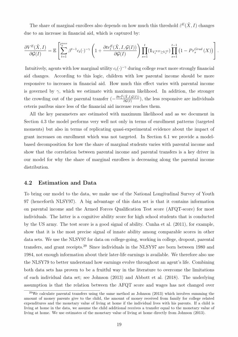
ure 5(a) provides the answer: revenue-maximizing financial aid in this case is very progressiveas well. Whereas the overall level of financial aid is naturally lower if the consumption utility ofstudents is not valued, the declining pattern is basically unaffected. For lower parental incomelevels, revenue-maximizing aid is more generous than the current schedule, which implies thatan increase must be more than self-financing. We study this in more detail in Section 5.4.The implied graduation patterns are illustrated in Figure 5(b).
5.4 Self-Financing Reforms
An increase in financial aid can be self-financing if properly targeted. The solid red line inFigure 6 illustrates the fiscal return, that is, the net effect on government revenue were financialaid for a particular income level to be increased by $1. For example, a 40% return implies thatthe net present value increase in tax revenue is 40% larger than the cost of increasing financialaid. Returns are positive for parental income between $0 and $33,000; the latter numbercorresponds to the 32nd percentile of the parental income distribution. This result is striking:increasing subsidies for this group is a free lunch. An alternative would be to consider reformswhere financial aid is increased for students below a certain parental income level. This caseis illustrated by the dashed-dotted blue line in Figure 6. An increase in financial aid targetedto children with parental income below $54,000 – corresponding to the 59th percentile – isslightly above the margin of being self-financing.
27

(a) Financial Aid (b) Graduation Rates
Figure 5: Tax-Revenue-Maximizing Financial Aid Policies
Notes: The dashed-dotted (blue) line shows the optimal schedule under the objective of maximizingnet-tax revenue (net of expenditures for financial aid). Optimal financial aid with a Utilitarianwelfare function and current financial aid are also shown for comparison in Panel (a). In Panel (b)we display the college graduation share by parental income group for each of the three scenarios.
6 Why Are Optimal Policies Progressive?
We have just shown in Section 5 that optimal financial aid is progressive and more so thanthe current US policies. In Sections 5.2 and 5.3, we have also shown that the results are notdriven by the desire to redistribute from richer to poorer students. We now explore the keyforces determining this progressivity result. Recall that the change in welfare due to a smallincrease of G(I) is given by (3)
@E(I)
@G(I) ⇥�T E(I)| {z }Enrollment Effect
+@C(I)
@G(I)
�����E(I)
E(I)⇥�T C(I)
| {z }Completion Effect
� E(I)�1�W
E(I)�
| {z }Mechanical Effect
.
To explain why the optimal financial aid schedule is more progressive than the current USfinancial aid, we illustrate the two most important determinants of this welfare effect: theenrollment effect and the mechanical effect evaluated at the current US system financial aid.We only found a quantitatively very small contribution of the completion effect and thereforefocus on the other two effects. Figure 7(a) plots the increase in enrollment for a $1,000 increasestarting from the current financial aid system against parental income. The curve is decreasingin income – children with low parental income react more strongly. This contributes to theresult that optimal financial aid is more progressive than the current US benchmark. Bycontrast, the fiscal externality �T E(I) is increasing in parental income because (i) marginal
28
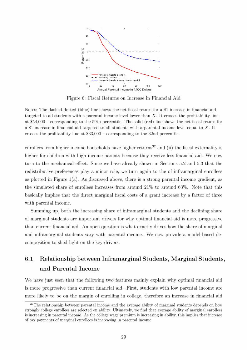
Figure 6: Fiscal Returns on Increase in Financial Aid
Notes: The dashed-dotted (blue) line shows the net fiscal return for a $1 increase in financial aidtargeted to all students with a parental income level lower than X. It crosses the profitability lineat $54,000 – corresponding to the 59th percentile. The solid (red) line shows the net fiscal return fora $1 increase in financial aid targeted to all students with a parental income level equal to X. Itcrosses the profitability line at $33,000 – corresponding to the 32nd percentile.
enrollees from higher income households have higher returns37 and (ii) the fiscal externality ishigher for children with high income parents because they receive less financial aid. We nowturn to the mechanical effect. Since we have already shown in Sections 5.2 and 5.3 that theredistributive preferences play a minor role, we turn again to the of inframarginal enrolleesas plotted in Figure 1(a). As discussed above, there is a strong parental income gradient, asthe simulated share of enrollees increases from around 21% to around 63%. Note that thisbasically implies that the direct marginal fiscal costs of a grant increase by a factor of threewith parental income.
Summing up, both the increasing share of inframarginal students and the declining shareof marginal students are important drivers for why optimal financial aid is more progressivethan current financial aid. An open question is what exactly drives how the share of marginaland inframarginal students vary with parental income. We now provide a model-based de-composition to shed light on the key drivers.
6.1 Relationship between Inframarginal Students, Marginal Students,
and Parental Income
We have just seen that the following two features mainly explain why optimal financial aidis more progressive than current financial aid. First, students with low parental income aremore likely to be on the margin of enrolling in college, therefore an increase in financial aid
37The relationship between parental income and the average ability of marginal students depends on howstrongly college enrollees are selected on ability. Ultimately, we find that average ability of marginal enrolleesis increasing in parental income. As the college wage premium is increasing in ability, this implies that increaseof tax payments of marginal enrollees is increasing in parental income.
29

(a) Marginal Students (b) Fiscal Externality
Figure 7: Marginal Students and Tax Revenue Changes
Notes: In (a), we plot the change in enrollment rates for a simulated $1,000 change in financial aidfor each parental income level. The average (across all individuals in the sample) is 1.69 percentagepoints. In (b), we show the implied average fiscal externality across all students who are marginalw.r.t. the financial aid increase.
targeted at low income families will induce larger increases in college enrollment. Second, thepositive relation between college enrollment and parental income is strong and therefore thedirect fiscal costs of increasing financial aid is lower for children with low parental income.We now perform a model-based decomposition exercise to better understand which factorsdrive these two relationships. For this decomposition, all changes to the model specificationare cumulative. That is, each new model specification contains the same model alterations asthe previous specification.38
To isolate the effects of model primitives, we perform this decomposition for a hypotheticalflat financial aid schedule instead of the current US tax schedule. This allows us to isolatethe influence of the model primitives, instead of mixing the effects of current policies andmodel primitives. Specifically, we set the aid for all parental income groups to the mean levelof financial aid in the data. Results are similar if the decomposition is performed for thecurrent financial aid system, as we document in Appendix C.1. We start by focusing on therelationship between parental income and college enrollment in Figure 8(a).39 The solid linecaptures the baseline case. College enrollment rates are strongly increasing in parental income:69% of students at the top of the parental income distribution enroll in college compared toonly 17% at the bottom of the distribution.40 One factor that leads to this positive relationshipis the correlation between parental income and ability. To understand the contribution of this
38In Appendix C.2, we consider an alternative decomposition in which we equalize parental transfers first.In Appendix C.3, we consider a decomposition where we remove the borrowing constraint before we equalizeparental transfers.
39Alternatively, we could have focused on graduation instead of enrollment. The implications are verysimilar.
40Note that this relationship is stronger than the one in Figure 1(a) where the current financial aid scheduleis used as benchmark.
30

correlation toward differential college-going rates by parental income, we simulate a version ofthe model in which we remove the correlation between parental income and ability by drawingeach agent’s ability from the unconditional ability distribution. Recall that ability affectsboth the returns to college and the psychic costs of attending college. Figure 8(a) shows thatthe relation between college enrollment and parental income reduces substantially, with 27%of children at the bottom of the income distribution enrolling in college compared to 69% ofchildren from the top of the income distribution.
Additionally, children with higher parental income are more likely to go to college becauseparental income is positively correlated with parental education. Since higher parental edu-cation lowers psychic costs, this implies a negative correlation between parental income andpsychic costs. We remove the relation between parental education and psychic costs in collegeby setting ParEd = 0, in addition to removing the correlation between parental income andability.41 After removing these differences in psychic costs, the relationship between parentalincome and college enrollment becomes again flatter with 33% of children from the bottom ofthe income distribution and 48% from the top of the income distribution.
In our model, there are further factors that influence the parental income gradient in collegeeducation. The individual returns to college are not known at the time of the enrollmentdecision. As individuals are risk averse and as parents with higher income levels give highertransfers for students attending college, this riskiness of college is another mechanism whichcan generate a positive relationship between college and parental income. In addition to themodifications above, we remove this risk in the monetary return to college by simulating aversion of the model in which each agent with certainty receives a fixed labor market abilitydraw. Removing the riskiness of college leads to a further flattening of the relationship betweenparental income and college enrollment. Yet there is still a gradient as enrollment increasesfrom 35% to 48% due to the fact that high parental income children obtain more transfers fromtheir parents. We finally remove this relationship by providing all children the mean parentaltransfer levels for enrollees and non-enrollees and assuming that no families are eligible forsubsidized Stafford loans. As a consequence, the relationship between parental income andcollege enrollment becomes flat.42 We conclude that all components play an important rolefor the increasing share of inframarginal students with the exception of the risk channel.
We turn to the determinants of the negative relation between parental income and share ofmarginal enrollees (again considering a $1,000 increase in financial aid) in Figure 8(b). Thesolid line shows the relationship between parental income and the share of marginal studentsin the baseline case. The share of marginal students is decreasing in parental income. Thedotted line and the dash-dotted line show the cases in which we remove the correlation between
41Furthermore, we set 0 so that the average psychic cost of going to college is unchanged.42The fact that it is not totally flat is due to the fact that individuals still differ in gender and region and
these variables are not distributed in exactly the same way for each parental income group.
31
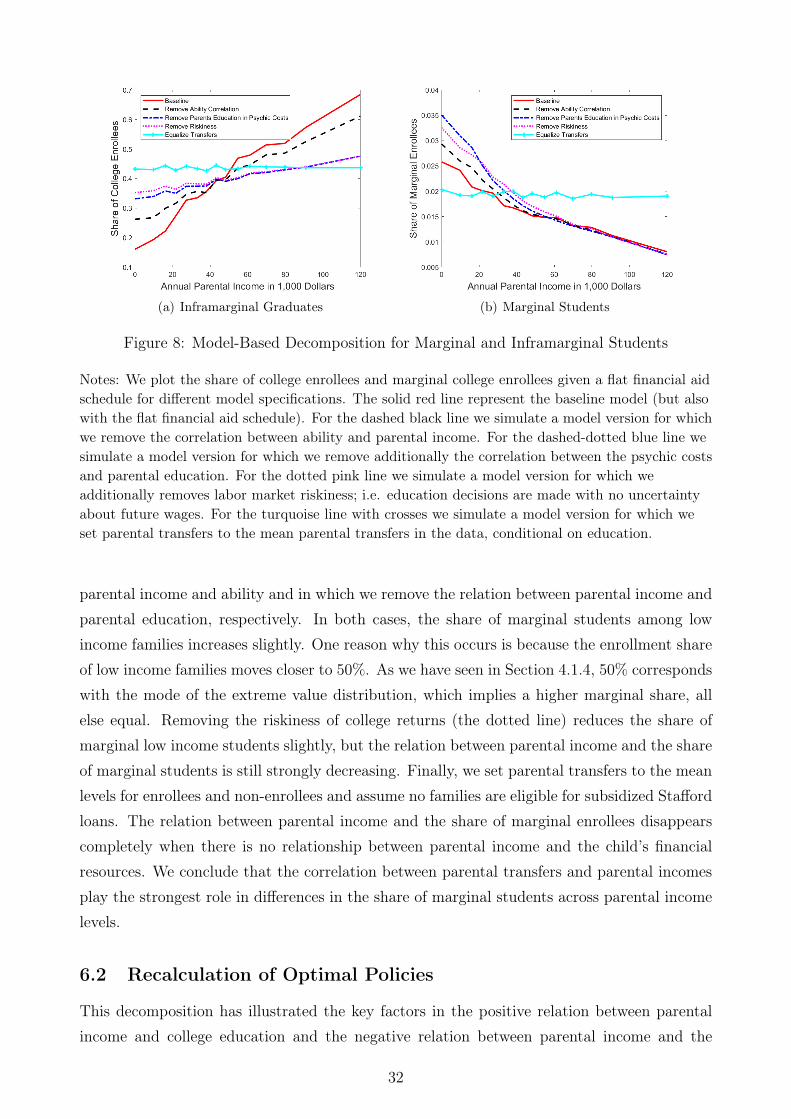
(a) Inframarginal Graduates (b) Marginal Students
Figure 8: Model-Based Decomposition for Marginal and Inframarginal Students
Notes: We plot the share of college enrollees and marginal college enrollees given a flat financial aidschedule for different model specifications. The solid red line represent the baseline model (but alsowith the flat financial aid schedule). For the dashed black line we simulate a model version for whichwe remove the correlation between ability and parental income. For the dashed-dotted blue line wesimulate a model version for which we remove additionally the correlation between the psychic costsand parental education. For the dotted pink line we simulate a model version for which weadditionally removes labor market riskiness; i.e. education decisions are made with no uncertaintyabout future wages. For the turquoise line with crosses we simulate a model version for which weset parental transfers to the mean parental transfers in the data, conditional on education.
parental income and ability and in which we remove the relation between parental income andparental education, respectively. In both cases, the share of marginal students among lowincome families increases slightly. One reason why this occurs is because the enrollment shareof low income families moves closer to 50%. As we have seen in Section 4.1.4, 50% correspondswith the mode of the extreme value distribution, which implies a higher marginal share, allelse equal. Removing the riskiness of college returns (the dotted line) reduces the share ofmarginal low income students slightly, but the relation between parental income and the shareof marginal students is still strongly decreasing. Finally, we set parental transfers to the meanlevels for enrollees and non-enrollees and assume no families are eligible for subsidized Staffordloans. The relation between parental income and the share of marginal enrollees disappearscompletely when there is no relationship between parental income and the child’s financialresources. We conclude that the correlation between parental transfers and parental incomesplay the strongest role in differences in the share of marginal students across parental incomelevels.
6.2 Recalculation of Optimal Policies
This decomposition has illustrated the key factors in the positive relation between parentalincome and college education and the negative relation between parental income and the
32

Figure 9: Optimal Financial Aid for Different Model Specifications
Notes: For each model specification (see Figure 8), we illustrate the respective optimal financial aidschedule.
share of marginal students. Removing the different elements from the model also affects theother forces that determine the optimal financial aid schedule. To get the complete picture,we therefore now simulate the respective optimal financial aid schedule for all these modelspecifications. Figure 9 shows the implied optimal policies for each model specification. First,the positive relation of parental income with ability and parental education are not the maindrivers of the financial aid results. Although graduation rates flatten (see the lines in Figure8(a)), there are offsetting effect as low-income children are now more likely to be marginal(see the lines in Figure 8(b)). Policies are still relatively progressive in those models.
Removing riskiness in addition has a stronger impact, because there are no offsetting effectsin this case. Both the inframarginal and marginal schedule are flatter now. Finally, theturquoise crossed line shows an almost zero slope, as transfers are equalized and we are ina world where parental income plays no more role. The effects for marginal students andinframarginal students again work in tandem, pushing towards flat aid.43
From this decomposition, we conclude that the correlations between parental income andparental transfers, psychic costs, and ability all play important roles in the progressive opti-mal aid schedule with parental transfers probably playing the biggest role. The correlation ofparental income with parental transfers drives the negative correlation of parental income andshare of marginal students and also plays a role in the positive correlation of parental incomeand the share of inframarginal students. The relationships between parental income and abilityand psychic costs play important roles in the correlation between share of inframarginal stu-dents and parental income, and therefore also play important roles in the progressive optimalaid schedule.44
43Again, the fact that it financial aid not totally flat is due to the fact that individuals still differ in genderand region and these variables are not distributed in exactly the same way for each parental income group.
44In Appendix C.2 we consider a decomposition in which we first remove the correlation with parentaltransfers before removing the correlations with ability and psychic costs. We reach similar conclusions. InAppendix C.3, we consider a decomposition which is as in the main body but we also remove borrowing
33

7 Extensions
We consider five important extensions: the role of borrowing constraints, endogenous abilitiesof children, general equilibrium effects, endogenous optimal taxation, and merit-based aid.The latter three are found in the appendix, because of space constraints. General equilibriumeffects can be found in Appendix C.8, endogenous optimal taxation can be found in AppendixC.9, and merit-based aid can be found in Appendix C.10.
7.1 The Role of Borrowing Constraints
We have shown that optimal progressivity is not primarily driven by redistributive tastes butrather by efficiency considerations in Section 5.3. Given that our analysis assumes that stu-dents cannot borrow more than the Stafford Loan limit, the question arises whether theseefficiency considerations are driven by borrowing limits that should be particularly bindingfor low-parental-income children. To elaborate on this question, we ask how normative pre-scriptions for financial aid policies change if students can suddenly borrow as much as theywant (up to the natural borrowing limit, which is not binding). For this thought experiment,we first remove borrowing constraints and keep the current financial aid system. This willincrease college enrollment and imply a windfall fiscal gain for the government. In a secondstep, we choose optimal financial aid but restrict the government to not use this windfall gain.As we show in Section C.4, optimal financial aid policies become less progressive in this case.This is expected. More low-income children are close to the borrowing constraint in the base-line specification. When we remove borrowing constraints, redistributing funds towards thesestudents becomes less attractive for the utilitarian social planner. Quantitatively, however,optimal policies are still very progressive even when borrowing constraints are removed. Wealso re-estimated a version of the model in which borrowing constraints varied by parentalresources. We found that the optimal financial aid schedule was very similar to the baselineschedule. Details can be found in Appendix C.5. We also considered alternative unreportedversions, where exogenous borrowing constraints depend differently on characteristics of thechild and the parent. The policy implications were not affected much.
7.2 Endogenous Ability
Up to this point, we have assumed that a child’s ability at the beginning of the model, ✓,is exogenous. One might be concerned that parents may respond to changes in the financialaid schedule by adjusting their investment in their child’s development, therefore changingtheir child’s ability at the time of the college entrance decision. To better understand how theoptimal financial aid schedule would differ if ability were endogenous with respect to financial
constraints as an intermediate case before removing parental transfers. In this case the role of parentaltransfers is much more limited.
34

aid, we posit a model extension in which a child’s ability is determined endogenously as afunction of parental investment.
Children are endowed with an initial ability at birth ✓0, where ✓0 is a random variable withCDF ✓0 ⇠ F✓0(·|I). A child’s ability at the time of college, ✓, is produced as a function of thechild’s initial ability and parental monetary investment, Invest. The parent observes ✓0 atthe beginning of the child’s life and then chooses investment in the child. Additionally, theparent chooses parental transfers when the child attends college, as in the baseline model. Forsimplicity, we assume that grants are only a function of income when solving the model withendogenous ability. This considerable simplifies the model solution.
For the production of the child’s ability, we assume the following functional form, which isvery similar to and based on the translog functional form employed in Agostinelli and Wiswall(2016)45
✓ = lnA+ �1 ln ✓0 + �2 ln Invest+ �3 ln ✓0 ln Invest+ ◆,
where ◆ is a normally distributed error that is unknown by the parent at the time of choosingInvest, and where A, �1, �2, and �3 are parameters of the ability production function. Afterthe parent chooses Invest, the ability production shock ◆ is realized. The parent’s problemis then the same as in the baseline case: each year, the parent continues to make consump-tion/saving decisions and chooses a parental transfer schedule when the agent reaches thecollege enrollment choice. Therefore, increases in early childhood investment increase thechild’s expected ability, but come at the cost of reduced consumption for the parent andpotentially lower transfers when the child reaches the enrollment decision.
We calibrate the parameters of the childhood ability production function to match the jointdistribution of parental income and ability we observe in our data and selected moments fromAgostinelli and Wiswall (2016). Details on the calibration are included in Appendix C.6. Dahland Lochner (2012) use changes in the EITC to instrument for family income and find thata $1000 increase in family income leads to an increase in ability scores by 6% of a standarddeviation. We simulate an increase in yearly family income of parents by $1,000 in our model.The increase in income leads to an average increase in AFQT scores of 2.2% of a standarddeviation across all children, and an increase of 5.1% of a standard deviation for children inthe lowest quintile. Therefore, the simulated responsiveness of ability with respect to parentalincome is slightly smaller than but in line with Dahl and Lochner (2012).
The optimal financial aid schedule, graduation rates, and ability levels with endogenousability are shown in Figure 10. Panel 10(a) shows the new optimal financial aid schedulewhen ability is endogenous. Compared to the baseline case when ability is exogenous, the
45Agostinelli and Wiswall (2016) estimate a model of early childhood developments with multiple periodsin which childhood skills are latent. Additionally, they use a broader concept of parental investment; theinvestment we refer to here is strictly monetary.
35

optimal aid schedule is now much higher, reflecting that increases in financial aid are now muchmore profitable for the government. With endogenous ability, increases in financial aid leadto increases in child ability, which increase tax payments of both marginal and inframarginalchildren. The optimal aid schedule is still highly progressive. Panel 10(b) shows the graduationrates evaluated at the optimal aid schedule with endogenous ability. Switching to the optimalschedule leads to an increase in college graduation rates of over 10%, reflecting that 1) theoptimal schedule is considerably more generous than the current schedule and 2) increases infinancial aid lead to larger increases in college-going when ability is endogenous.46
(a) Financial Aid (b) Graduation Rates
Figure 10: Financial Aid and Graduation with Endogenous AbilityNotes: The dashed-dotted (blue) line shows the optimal schedule when child’s ability is endogenous.Optimal financial aid with exogenous ability and current financial aid are also shown for comparisonin Panel (a). In Panel (b) we display the college graduation share by parental income group whenability is endogenous with the optimal aid schedule and with the current aid schedule.
As emphasized by Caucutt and Lochner (2017) and Lee and Seshadri (2019), low incomeparents may face borrowing constraints when their child is young and therefore unable toadjust their investment in their child’s ability in response to changes in education policy.In Appendix C.7, we calculate the optimal aid schedule with endogenous ability under theassumption that low income parents may be borrowing constrained when their child is young.We find that the optimal progressivity of the system decreases as we increase the percentage oflow-education families who are borrowing constrained. However, the optimal schedule remainsmore progressive than the current schedule in all cases.
46We show the end of childhood ability as a function of parental income under the current financial aidschedule and under the optimal schedule in Section C.6. Switching to the optimal aid schedule leads tosubstantial increases in child ability, especially for children in the lower end of the parental income distribution.
36
8 Conclusion
This paper has analyzed the normative question of how to optimally design financial aidpolicies for students. We find that optimal financial aid policies are strongly progressive. Thisresult holds for different social welfare functions, assumptions on credit markets for students,and assumptions on income taxation. Moreover, we find that a progressive expansion infinancial aid policies could be self-financing through higher tax revenue, thus benefiting alltaxpayers as well as low-income students directly. It seems to be that financial aid policiesare a rare case with no classic equity-efficiency trade-off because a cost-effective targetingof financial aid goes hand in hand with goals of social mobility and redistribution. We alsothink that our results can be used for policy recommendations according to the criteria ofDiamond and Saez (2011):47 the economic mechanism is empirically relevant and of firstorder importance to the problem, it is very robust and progressive financial aid systems areclearly implementable, as they are universal across all OECD countries.
Future work could focus on adding heterogeneity in the quality of colleges, which wouldallow for rich interactions with financial aid policies. In such a setting, it would seem naturalto let the government optimize over financial aid as a joint function of parental background andcollege quality. In addition, college quality could adjust endogenously. Thinking more seriouslyabout these issues could also extend the scope of the analysis to the level of community colleges.We leave that for future research.
References
Abbott, B., G. Gallipoli, C. Meghir, and G. L. Violante (2018): “Education Policyand Intergenerational Transfers in Equilibrium,” Cowles Foundation Discussion Paper No.1887R.
Agostinelli, F. and M. Wiswall (2016): “Estimating the Technology of Children’s SkillFormation,” NBER Working Paper No. 22442.
Alsalam, N. (2013): “The Federal Pell Grant Program: Recent Growth and Policy Options,”Washington, DC: Congressional Budget Office.
Altonji, J. G., P. Bharadwaj, and F. Lange (2012): “Changes in the Characteristicsof American Youth: Implications for Adult Outcomes,” Journal of Labor Economics, 30,783–828.
Altonji, J. G. and T. A. Dunn (1996): “The Effects of Family Characteristics on theReturn to Education,” Review of Economics and Statistics, 78, 692–704.
Bagnoli, M. and T. Bergstrom (2005): “Log-Concave Probability and Its Applications,”Economic Theory, 26, 445–469.47Diamond and Saez (2011) write in their abstract: "We argue that a result from basic research is relevant
for policy only if (a) it is based on economic mechanisms that are empirically relevant and first order to theproblem, (b) it is reasonably robust to changes in the modeling assumptions, (c) the policy prescription isimplementable (i.e., is socially acceptable and is not too complex)."
37

Baum, S., J. Ma, and K. Payea (2013): Education Pays, 2013: The Benefits of HigherEducation for Individuals and Society. Trends in Higher Education Series., New York: TheCollege Board.
Blau, F. D. and L. M. Kahn (2007): “Changes in the Labor Supply Behavior of MarriedWomen: 1980–2000,” Journal of Labor Economics, 25, 393–438.
Bohacek, R. and M. Kapicka (2008): “Optimal Human Capital Policies,” Journal ofMonetary Economics, 55, 1–16.
Bovenberg, A. L. and B. Jacobs (2005): “Redistribution and Education Subsidies AreSiamese Twins,” Journal of Public Economics, 89, 2005–2035.
Card, D. (1999): “The Causal Effect of Education on Earnings,” Handbook of Labor Eco-nomics, 3, 1801–1863.
Card, D. and T. Lemieux (2001): “Can Falling Supply Explain the Rising Return to Collegefor Younger Men? A Cohort-Based Analysis,” The Quarterly Journal of Economics, 116,705–746.
Carneiro, P. and J. J. Heckman (2003): “Human Capital Policy,” IZA Discussion PaperNo. 821.
Carroll, S. J. and E. Erkut (2009): The Benefits to Taxpayers from Increases in Students’Educational Attainment, vol. 686, Santa Monica, CA: RAND Corporation.
Castleman, B. L. and B. T. Long (2016): “Looking beyond Enrollment: The CausalEffect of Need-Based Grants on College Access, Persistence, and Graduation,” Journal ofLabor Economics, 34, 1023–1073.
Caucutt, E. M. and L. Lochner (2017): “Early and Late Human Capital Investments,Borrowing Constraints, and the Family,” Tech. rep.
College Board (2015): Trends in Student Aid 2015. Trends in Higher Education Series.,New York: The College Board.
Cunha, F., J. Heckman, and S. Navarro (2005): “Separating Uncertainty from Hetero-geneity in Life Cycle Earnings,” Oxford Economic Papers, 57, 191–261.
Cunha, F., F. Karahan, and I. Soares (2011): “Returns to Skills and the College Pre-mium,” Journal of Money, Credit and Banking, 43, 39–86.
Dahl, G. B. and L. Lochner (2012): “The Impact of Family Income on Child Achievement:Evidence from the Earned Income Tax Credit,” American Economic Review, 102, 1927–1956.
De Nardi, M. (2004): “Wealth Inequality and Intergenerational Links,” Review of EconomicStudies, 71, 743–768.
Deming, D. and S. Dynarski (2009): “Into College, Out of Poverty? Policies to Increasethe Postsecondary Attainment of the Poor,” NBER Working Paper 15387.
Diamond, P. A. and E. Saez (2011): “The Case for a Progressive Tax: From Basic Researchto Policy Recommendations,” Journal of Economic Perspectives, 25, 165–190.
Dynarski, S. M. (2003): “Does Aid Matter? Measuring the Effect of Student Aid on CollegeAttendance and Completion,” American Economic Review, 93, 279–288.
Findeisen, S. and D. Sachs (2016): “Education and Optimal Dynamic Taxation: The Roleof Income-Contingent Student Loans,” Journal of Public Economics, 138, 1–21.
38

——— (2017): “Redistribution and Insurance with Simple Tax Instruments,” Journal of PublicEconomics, 146, 58–78.
Golosov, M., A. Tsyvinski, and N. Werquin (2014): “A Variational Approach to theAnalysis of Tax Systems,” Working Paper.
Guner, N., R. Kaygusuz, and G. Ventura (2014): “Income Taxation of US Households:Facts and Parametric Estimates,” Review of Economic Dynamics, 17, 559–581.
Heathcote, J., K. Storesletten, and G. L. Violante (2017): “Optimal Tax Progres-sivity: An Analytical Framework,” Quarterly Journal of Economics, 132, 1693–1754.
Heckman, J. J., L. Lochner, and C. Taber (1998): “Explaining Rising Wage Inequality:Explorations with a Dynamic General Equilibrium Model of Labor Earnings with Hetero-geneous Agents U,” Review of Economic Dynamics, 1, 158.
Heckman, J. J., L. J. Lochner, and P. E. Todd (2006): “Earnings Functions, Ratesof Return and Treatment Effects: The Mincer Equation and Beyond,” Handbook of theEconomics of Education, 1, 307–458.
Heckman, J. J. and S. Navarro (2007): “Dynamic discrete choice and dynamic treatmenteffects,” Journal of Econometrics, 136, 341–396.
Hilger, N. G. (2016): “Parental Job Loss and Children’s Long-Term Outcomes: Evidencefrom 7 Million Fathers’ Layoffs,” American Economic Journal: Applied Economics, 8, 247–283.
Jacobs, B. and U. Thuemmel (2018): “Optimal Taxation of Income and Human Capi-tal and Skill-Biased Technical Change,” Tech. rep., Mimeo, Tinbergen Institute, Amster-dam/Rotterdam.
Jacquet, L. and E. Lehmann (2016): “Optimal Taxation with Heterogeneous Skills andElasticities: Structural and Sufficient Statistics Approaches,” THEMA Working Paper 2016-04.
Jacquet, L., E. Lehmann, and B. Van der Linden (2013): “The Optimal Marginal TaxRates with Both Extensive and Intensive Responses,” Journal of Economic Theory, 148,1770–1805.
Johnson, M. T. (2013): “Borrowing Constraints, College Enrollment, and Delayed Entry,”Journal of Labor Economics, 31, 669–725.
Katz, L. F. and K. M. Murphy (1992): “Changes in Relative Wages, 1963–1987: Supplyand Demand Factors,” Quarterly Journal of Economics, 107, 35–78.
Kleven, H. J. (2018): “Sufficient Statistics Revisited,” Working Paper.
Koeniger, W. and J. Prat (2017): “Human Capital and Optimal Redistribution,” WorkingPaper.
Krueger, D. and A. Ludwig (2013): “Optimal Progressive Labor Income Taxation andEducation Subsidies When Education Decisions and Intergenerational Transfers Are En-dogenous,” American Economic Review: Papers & Proceedings, 103, 496–501.
——— (2016): “On the Optimal Provision of Social Insurance: Progressive Taxation versusEducation Subsidies in General Equilibrium,” Journal of Monetary Economics, 77, 72–98.
Laun, T. and J. Wallenius (2016): “Social Insurance and Retirement: a Cross-CountryPerspective,” Review of Economic Dynamics, 22, 72–92.
39

Lawson, N. (2017): “Liquidity Constraints, Fiscal Externalities and Optimal Tuition Subsi-dies,” American Economic Journal: Economic Policy, 8, 313–343.
Lee, D., S. Y. Lee, and Y. Shin (2017): “The Option Value of Human Capital: HigherEducation and Wage Inequality,” Working Paper.
Lee, S. Y. and A. Seshadri (2019): “On the intergenerational transmission of economicstatus,” Journal of Political Economy, 127, 855–921.
Lehmann, E., L. Simula, and A. Trannoy (2014): “Tax Me If You Can! OptimalNonlinear Income Tax between Competing Governments,” Quarterly Journal of Economics,129, 1995–2030.
Mirrlees, J. A. (1971): “An exploration in the theory of optimum income taxation,” TheReview of Economic Studies, 38, 175–208.
OECD (2014): “Education at a Glance 2014: OECD Indicators,” URL:http://dx.doi.org/10.1787/eag-2014-en.
Oreopoulos, P. and U. Petronijevic (2013): “Making College Worth It: A Review ofResearch on the Returns to Higher Education,” NBER Working Paper 19053.
Piketty, T. and E. Saez (2013): “Optimal Labor Income Taxation,” Handbook of PublicEconomics, Vol 5.
Saez, E. (2001): “Using Elasticities to Derive Optimal Income Tax Rates,” Review of Eco-nomic Studies, 68, 205–229.
——— (2002): “Optimal Income Transfer Programs: Intensive versus Extensive Labor SupplyResponses,” Quarterly Journal of Economics, 117, 1039–1073.
Saez, E. and S. Stantcheva (2016): “Generalized Social Marginal Welfare Weights forOptimal Tax Theory,” American Economic Review, 106, 24–45.
Shaked, M. and J. G. Shanthikumar (2007): Stochastic Orders, Springer Series in Statis-tics, New York: Springer.
Snyder, T. D. and C. M. Hoffman (2001): Digest of Education Statistics 2000, NationalCenter for Education Statistics.
Stantcheva, S. (2015): “Optimal Income, Education, and Bequest Taxes in an Intergener-ational Model,” NBER Working Paper No. 21177.
——— (2017): “Optimal Taxation and Human Capital Policies over the Life Cycle,” Journalof Political Economy, 125, 1931–1990.
Zimmerman, S. (2014): “The Returns to College Admission for Academically Marginal Stu-dents,” Journal of Labor Economics, 32, 711–754.
40

A Theoretical Appendix
A.1 Derivation of Equation 3
The Lagrangian for the government’s problem reads as:
L =
Z
R+
Z
�
max{V E(X, I), V H(X, I)}k(X, I)dXdI
+ ⇢
(Z
R+
Z
�
NT H
NPV(X, I)1V
E
j<V
H
j
k(X, I)dXdI
+
Z
R+
Z
�
NT G
NPV(X, I)1V
E
j�V
H
j
PC(X, I,G(I))k(X, I)dXdI
+
Z
R+
Z
�
NT D
NPV(X, I)1V
E
j�V
H
j
�1� P
C(X, I,G(I))�k(X, I)dXdI � F
).
The derivative w.r.t. G(I) is given by:
@L@G(I) =
Z
�
1VE
j�V
H
j
@VE(X, I)
@G(I) h(X|I)dX (9)
+ ⇢
Z
�
⇢P
C(X, I,G(I))@NT G
NPV(X, I)
@G(I) +�1� P
C(X, I,G(I))� @NT D
NPV(X, I)
@G(I)
�h(X|I)dX
+ ⇢
Z
�
1Hj!Ej
nP
C(X, I,G(I))NT G
NPV(X, I) +
�1� P
C(X, I,G(I))�NT D
NPV(X, I)
�NT H
NPV(X, I)
oh(X|I)dX
+ ⇢
Z
�
@PC(X, I,G(I))@G(I)
�NT G
NPV(X, I)�NT D
NPV(X, I)
�h(X|I)dX
Recall that 1Hj!Ejtakes the value one if an individual of type j is pushed over the college
enrollment margin due to a small increase in financial aid.The first term captures the direct utility increase of inframarginal enrollees due to receiving
more financial aid. The second term captures the direct fiscal effect of paying more financial aidto inframarginal students. The third term captures the fiscal effect of additional enrollees. Thefourth effect captures the fiscal effect due to the increase in the completion rate of inframarginalstudents. The implied change in the enrollment and dropout rate has no direct first-order effecton welfare: individuals that are marginal in their decision to enroll or not and to continuestudying or drop out, were just indifferent between the two respective options, hence thischange in behavior has no effect on their utility.
The definitions of E(I) and �TE(I) directly imply that the third term equals the enrollment
effect in (3) multiplied by ⇢. The definitions of �T C(I), E(I) and C(I) directly imply thatthe fourth term equals the completion effect in (3) multiplied by ⇢.
41

Now it remains to be shown that the first and second term are equal to the mechanicaleffect in (3). The application of the envelope theorem implies that the first term reads as
Z
�
1VE
j�V
H
j
E
2
4tmaxgX
t=1
�t�1
UE
c(·)✓1 +
@trE
t(·)
@G(I)
◆ tY
s=1
(1V NDs �V D
s)t�1Y
s=1
�1� Pr
Grad
s(X)
�3
5 h(X|I)dXE(I).
(10)The second term, using the definitions of NT G
NPV(X, I) and NT D
NPV(X, I), can be written
as
�⇢
Z
�
tmaxgX
t=1
1
1 + r
tY
s=1
PE
t(X, I,G(I))h(X|I)dX. (11)
Adding (10) and (11), using the definition of the social marginal welfare weight yields equation3.
A.2 More General Version of Equation 3 with Annual Dropout De-
cisions
We now show the generalization in which individuals can drop out each period. For this case,we have to distinguish between individuals that drop out in different periods. Hence, for theeducation decision we have: e 2 {H,G,D1, D2, ..., Dtmax
g}, where Dt implies that individuals
drop out at the beginning of year t. Accordingly we can define the net fiscal contribution ofan individual of type (X, I) that drops out in period t by NT Dt
NPV(X, I):
NT Dt
NPV(X, I) =
TX
s=t
✓1
1 + r
◆s�1
E (T (ys)|X, I,Dt)� G(I)t�1X
s=1
✓1
1 + r
◆s�1
.
We also have to define the net fiscal contribution of an individual that is enrolled in year tmax
g
NT Etmaxg
NPV(X, I) = Ptmax
g(X, I,G(I))NT G
NPV(X, I) +
�1� Ptmax
g(X, I,G(I))
�NT Dt
maxg
NPV(X, I)
and for t = 2, 3, ..., tmax
g� 1:
NT Et
NPV(X, I) = Pt(X, I,G(I))NT Et+1
NPV(X, I) + (1� Pt(X, I,G(I)))NT Dt
NPV(X, I).
42

The Lagrangian for the government’s problem reads as:
L =
Z
R+
Z
�
max{V E(X, I), V H(X, I)}k(X, I)dXdI
+ ⇢
(Z
R+
Z
�
NT H
NPV(X, I)1V
E
j<V
H
j
k(X, I)dXdI
+
Z
R+
Z
�
NT G
NPV(X, I)1V
E
j�V
H
j
PC(X, I,G(I))k(X, I)dXdI
+
tmaxgX
⌧=1
"Z
R+
Z
�
NT D⌧
NPV(X, I)1V
E
j�V
H
j
⌧�1Y
t=1
Pt(X, I,G(I)) (1� P⌧ (X, I,G(I))) k(X, I)dXdI
#� F
).
The FOC for G(I) shares the same basic structure as (9). However, here the fiscal effects dueto change in dropout behavior are more involved:48
⇢
Z
�
tmaxg �1Y
t=1
Pt(X, I,G(I))@Ptmax
g(X, I,G(I))@G(I)
⇣NT G
NPV(X, I)�NT Dt
maxg
NPV(X, I)
⌘h(X|I)dX
+⇢
tmaxg �1X
⌧=1
"Z
�
⌧�1Y
t=1
Pt(X, I,G(I))@P⌧ (X, I,G(I))@G(I)
�NT E⌧+1
NPV(X, I)�NT D⌧
NPV(X, I)
�h(X|I)dX
#,
where we let P0(X, I,G(I)) = 1.In short term notation, similar to that in (3), we can write
tmaxgX
t=1
@Cont(I)
@G(I)
�����Et(I)
�T Con,t(I)Et(I)
where Cont(I) is the share of those enrollees with parental income I in period t, that continuestudying to year t+ 1. It is defined by
Cont(I) =Et+1(I)
Et(I)
for t = 1, 2, .., tmax
g� 1 and
Contmaxg
(I) =
R�1V
E
j�V
H
j
Qtmaxg
s=1 Ps(X, I,G(I))h(X|I)dXEtmax
g(I)
.
whereE1(I) = E(I) =
Z
�
1VE
j�V
H
j
h(X|I)dX.
and
Et(I) =
Z
�
1VE
j�V
H
j
t�1Y
s=1
Ps(X, I,G(I))h(X|I)dX.
48Again, changes in dropout behaviour have no direct welfare effect due to the envelope theorem.
43

Finally, the changes in tax revenue are defined by:
�T Con,t(I) =
R��T Con,t(X, I)@P (X,I,G(I))
@G(I) h(X|I)dXR�
@P (X,I,G(I))@G(I) h(X|I)dX
where
�T Con,t(X, I) = NT Et
NPV(X, I)�NT Dt
NPV(X, I).
Hence, the equivalent to equation 3 is given by:
@E(I)
@G(I) ⇥�T E(I) +
tmaxgX
t=1
Et(I)@Cont(I)
@G(I)
�����Et(I)
�T Con,t(I)� E(I)�1�W
E(I)�.
A.3 Proof of Proposition 1
The government’s problem reads as
maxG(I)
Z
R+
Z✓(I)
✓
U ((1� ⌧)yH) dH(✓|I)dF (I)
+
Z
R+
Z✓
✓(I)
U (((1� ⌧yH) (1 + ✓)� (F � G(I)� tr(I)))) dH(✓|I)dF (I)
+ �
"Z
R+
Z✓(I)
✓
⌧yH dH(✓|I)dF (I) +
Z
R+
Z✓
✓(I)
(⌧yH (1 + ✓)� G(I)) dH(✓|I)dF (I)� F
#,
where, as in Section 2, H and F denote the distributions of Pareto weights which integrate upto one and F is some exogenous revenue requirement. All Pareto weights are non-negative.
The first-order condition for G(I) is given by:
h(✓(I)|I)���@✓(I)
@G(I)
���⇣⌧yh✓(I)� G(I)
⌘�⇣1�H(✓(I)|I)
⌘(1�W
E(I)) = 0, (12)
where WE(I) is average social marginal welfare weight for enrollees with parental income I
and formally given by:
WE(I) =
R✓
✓U
0 (((1� ⌧yH) (1 + ✓)� (F � G(I)� tr(I)))) dH(✓|I)f(I)�(1�H(✓|I))f(✓) .
Using@✓(I)
@G(I) = � 1
yH(1� ⌧)
44

and inserting into (12) gives the first-order condition explained in the main text just beforeProposition 1. Solving for G(I) gives Proposition 1.
Unweighted Utilitarianism with U(x)=x. If we assume h(✓|I) = h(✓|I) for all (✓, I)and further assume U(x) = x, then, we obtain
WE(I) =
1
�8 I,
hence the welfare weights are the same for all parental income groups. The value for � ismeasures the marginal value of public funds and therefore depends on F . To get an under-standing of the optimal value for �, consider the perturbation around the optimum, whereG(I) is increased by � ! 0 for all I. This basically implies changing the lump sum componentof G(I) and is equivalent to just integrating over (12). The impact on welfare is given by:
Z
I
(1�WE(I))
⇣1�H(✓(I)|I)
⌘dF (I) +
Z
I
h(✓(I)|I)���@✓(I)
@G(I)
���⇣⌧yh✓(I)� G(I)
⌘dF (I) = 0.
and hence for WE(I) = 1�8 I:
Z
I
✓1� 1
�
◆⇣1�H(✓(I)|I)
⌘dF (I) +
Z
I
h(✓(I)|I)���@✓(I)
@G(I)
���⇣⌧yh✓(I)� G(I)
⌘dF (I) = 0.
Here we see that � = 1 would be consistent with G(I) = ⌧yh✓(I) for all I. Recall that thegovernment budget constraint is given by:
Z
R+
Z✓(I)
✓
⌧yH dH(✓|I)dF (I) +
Z
R+
Z✓
✓(I)
(⌧yH (1 + ✓)� G(I)) dH(✓|I)dF (I)� F = 0.
If the exogenous revenue requirement F is such that the budget constraint holds for G(I) =⌧yh✓(I) for all I, then we obtain � = 1 and the formula in Proposition 1 becomes
G(I) = ⌧ (F � tr(I)) . (13)
Assume that instead the budget constraint would be violated and this level of financial aidcan not be financed. Then we have � > 1 and hence W
E(I) < 1 8 I. Generally, we could alsohave the case where � < 1. E.g. assume that F = �1. In this case, there would be infinitelymany public funds available for financial aid and therefore the marginal value of public fundswould be zero. But of course this is only of theoretical interest.
The fact that the marginal value of public funds is not equal to unity even though pref-erences are linear may seem in contrast to the optimal income tax literature, where it is a
45

standard result that the marginal value of public funds is equal to one for quasi-linear pref-erences and in other words the average welfare weights is equal to one, see e.g. Saez (2002).The reason is that the policy instruments that we consider are such that there is no lumpsum element. While the financial aid schedule G(I) of course has an intercept G(0) that canoptimally be chosen, this is no lump sum transfer in the classical sense because it only reachescollege students and not individuals who forgo college. Therefore, varying this lump sumcomponent also has incentive effects on the college decision and one cannot just pay out adollar to everyone without affecting behavior.
A.4 Proof of Corollary 1
Differentiating (5) w.r.t. I yields:
G 0(I) = �⌧ tr0(I) + (1� ⌧)
@
⇣1�H(✓(I))
h(✓(I))
⌘
@✓(I)(tr0(I) + G 0(I)) (1�W
E)
where we used ✓(I) = F�tr(I)�G(I)(1�⌧)yH
. and therefore ✓0(I) = �tr
0(I)�G0(I)(1�⌧)yH
. Solving for G 0(I) weget
G 0(I) =�⌧ tr
0(I) + (1� ⌧)@
⇣1�H(✓(I))
h(✓(I))
⌘
@✓(I)tr
0(I)(1�WE)
1� (1� ⌧)@
⇣1�H(✓(I))
h(✓(I))
⌘
@✓(I)(1�WE)
which proves Corollary 1 since by assumption tr0(I) > 0 and log concavity of the skill distri-
bution implies@
⇣1�H(✓(I))
h(✓(I))
⌘
@✓(I)< 0.
A.5 Proof of Corollary 2
Differentiating (5) w.r.t. I yields:
G 0(I) = �⌧ tr0(I)+(1�W
E) (1� ⌧)
2
4@
⇣1�H(✓(I)|I)h(✓(I)|I)
⌘
@✓(I)(tr0(I) + G 0(I))� yH (1� ⌧)
@
⇣1�H(✓|I)h(✓|I)
⌘
@I
�����✓=✓(I)
3
5
Hence we obtain
G 0(I) =
�⌧ tr0(I) + (1�W
E) (1� ⌧)
2
4@
⇣1�H(✓(I))
h(✓(I))
⌘
@✓(I)tr
0(I)� yH (1� ⌧)@( 1�H(✓|I)
h(✓|I) )@I
�����✓=✓(I)
3
5
1� (1� ⌧)@
⇣1�H(✓(I))
h(✓(I))
⌘
@✓(I)(1�WE)
46

which proves Corollary 2 since by assumption tr0(I) > 0, log concavity of the skill distribution
implies@
⇣1�H(✓(I))
h(✓(I))
⌘
@✓(I)< 0 and we assumed
@
⇣1�H(✓|I)h(✓|I)
⌘
@I> 0 8 ✓, I.
A.6 Optimal Income Taxation
The planner’s problem is the same as in (1) with the difference that the planner also optimallychooses the income tax schedule T (·). Notice that the formula for optimal financial aid policiesis unaltered. We allow the tax function T (·) to be arbitrarily nonlinear in the spirit of Mirrlees(1971). We restrict the tax function to be only a function of income and to be independentof the education decision. This tax problem can either be tackled with a variational or taxperturbation approach (Saez, 2001; Golosov et al., 2014; Jacquet and Lehmann, 2016) or witha restricted mechanism design approach for nonlinear history-independent income taxes thatwe explore in Findeisen and Sachs (2017).
We here provide a heuristic version of the former approach within our model. For notationalconvenience, we consider the model of Section 2 with the assumption that individuals can onlydropout at the beginning of period 3. We also assume that agents can only graduate in 4 years.
Consider an increase of the marginal tax by an infinitesimal amount dT 0 in an incomeinterval of infinitesimal length [y⇤, y⇤ + dy]. As a consequence of this reform, all individualswith y > y
⇤ face an increase of the absolute tax level of dT 0dy. The tax reform therefore
induces a mechanical increase in welfare of
�WMR(y⇤) = ⇢dT 0
dy
TX
t=1
✓1
1 + r
◆t�1 Z 1
y⇤ht,H(y)dy ⇥ sH
+ ⇢dT 0dy
TX
t=3
✓1
1 + r
◆t�1 Z 1
y⇤ht,D(y)dy ⇥ sD
+ ⇢dT 0dy
TX
t=5
✓1
1 + r
◆t�1 Z 1
y⇤ht,G(y)dy ⇥ sG
through the tax revenue increase (in net present value). ht,e(y) is the density of income ofindividuals with education level e in period t and se is the overall share of individuals witheducation level e. Both, the income densities and the education shares are endogeneous w.r.t.to taxes, we get to this below.
47

Note that this increase in tax payment also has mechanical effects on individual utilitieswhich adds up to the following welfare effect
�WMU(y⇤) = dT 0
dy
TX
t=1
✓1
1 + r
◆t�1 Z 1
y⇤E (Uc|yt = y)ht,H(y)dy ⇥ sH
+ dT 0dy
TX
t=3
✓1
1 + r
◆t�1 Z 1
y⇤E (Uc|yt = y)ht,D(y)dy ⇥ sD
+ dT 0dy
TX
t=5
✓1
1 + r
◆t�1 Z 1
y⇤E (Uc|yt = y)ht,G(y)dy ⇥ sG.
Now we turn to the endogeneity of education shares. First of all some individuals will changetheir initial enrollment decision. We define 1y
⇤
Hj!Ejto take the value one if an individual of
type j is marginal in the enrollment decision w.r.t. to a one dollar tax increase for earningsabove y
⇤. Then, the welfare effect of individuals changing their enrollment decision due to asmall increase in T
0(y⇤) is given by:
�WE(y⇤) = ⇢dT 0
dy
Z
R+
Z
�
1y⇤
Hj!Ej
nNT E
NPV(X, I)�NT H
NPV(X, I)
oh(X|I)dXdI.
Similarly, the probability to continue college and not drop out is endogenous w.r.t. taxes, i.e.we have P (X, I,G(I), T (·)). The change in welfare due to the change in dropout behavior,with some abuse of notation, is simply given by:
�WD(y⇤) = ⇢
Z
R+
Z
�
Z 1
y⇤
@P (X, I,G(I), T (·))@T (y)
dy�NT G
NPV(X, I)�NT D
NPV(X, I)
h(X|I)dXdI.
Finally, an increase in the marginal tax rate also affects labor supply behavior for individualswithin the interval [y⇤, y⇤+dy]. Individuals within this infinitesimal interval change their laborsupply by
@y⇤t
@T 0dT0 = �"y⇤
t,1�T 0
y⇤t
1� T 0dT0.
Whereas this change in labor supply has no first-order effect on welfare via individual utilitiesby the envelope theorem, it has an effect on tax revenue, which is given by:
�WL(y⇤) =
T 0(y⇤)
1� T 0(y⇤)y⇤"y,1�T 0 ⇥ dT 0⇥
sH
TX
t=1
✓1
1 + r
◆t�1
ht,H(y⇤) + sD
TX
t=3
✓1
1 + r
◆t�1
ht,D(y⇤) + sG
TX
t=5
✓1
1 + r
◆t�1
ht,G(y⇤)
!.
Since this reform must not have any non-zero effect on welfare if the tax system is optimal,we have to have
48

�WMR(y⇤) +�WMU(y
⇤) +�WE(y⇤) +�WD(y
⇤) +�WL(y⇤) = 0 (14)
which provides an implicit characterization of T 0(y⇤).Finally, the optimal level for the lump-sum element of the tax schedule T (0) is implicitly
characterized by
�WMR(0) +�WMU(0) +�WE(0) +�WD(0) = 0.
This optimal tax approach is related to the formulas of Saez (2002) and Jacquet et al.(2013).
To implement this formula numerically, we follow a guess and verify approach. Hence, westart with a guess for the tax schedule and then evaluate (14).49 We then slightly adjustT
0(y⇤) to make (14) closer to zero (but keep �WMR(y⇤)+�WMU(y⇤)+�WE(y⇤)+�WD(y⇤)
fixed, i.e. we only adjust �WL(y⇤)). We then calculated the new allocation for this adjustedschedule and evaluate (14) for income levels again and so on. We proceed until convergence.50
B Estimation and Calibration
B.1 Current Tax Policies and Tuiton
To capture current tax policies, we use the approximation of Heathcote et al. (2017), whichhas been shown to work well in replicating the US tax code. Since this specification does notcontain a lump-sum element, we slightly adjust this schedule. We set the lump sum elementof the tax code T (0) to minus $1,800 a year. For average incomes this fits the deduction in theUS-tax code quite well.51 For low incomes this reflects that individuals might receive transferssuch as food stamps.52
For tuition costs, we take average values for the year 2000 from Snyder and Hoffman(2001) for the regions Northeast, North Central, South, and West, as they are defined in theNLSY. We also take into account the amount of money that is spent per student by publicappropriations, which has to be taken into account for the fiscal externality. The averagevalues are $7,434 for annual tuition and $4,157 for annual public appropriations per student.Besides these implicit subsidies, students receive explicit subsidies in the form of grants andtuition waivers. We estimate how this grant receipt varies with parental income and ability
49In fact a more complicated version of (14) which accounts for dropout behavior in every period and alsoaccounts for stochastic graduation.
50In each iteration, we also optimally choose the financial aid schedule G(I) given the tax schedule in therespective iteration.
51Guner et al. (2014) report a standard deduction of $7,350 for couples that file jointly. For an average taxrate of 25% this deduction could be interpreted as a lump sum transfer of slightly more than $1,800.
52The average amount of food stamps per eligible person was $72 per month in theyear 2000. Assuming a two person household gives roughly $1,800 per year. Source:http://www.fns.usda.gov/sites/default/files/pd/SNAPsummary.pdf
49

in Appendix B.2 using information provided in the NLSY97. We find a strong negative effectof parental income on financial aid receipt. Additionally, we can capture merit-based grantsby the conditional correlation of AFQT scores with grant receipt. Finally, we calibrate theexogenous budget element F in the following way. For the current U.S. polices, we calculatethe present value of financial aid spending and the present value of tax revenues collected fromthe cohorts that we consider (born between 1980 and 1984 from the NLSY97) and obtain F
from the difference between the two.We categorize the following 4 regions:
• Northeast: CT, ME, MA, NH, NJ, NY, PA, RI, VT
• North Central: IL, IN, IA, KS, MI, MN, MO, NE, OH, ND, SD, WI
• South: AL, AR, DE, DC, FL, GA, KY, LA, MD, MS, NC, OK, SC, TN , TX, VA, WV
• West: AK, AZ, CA, CO, HI, ID, MT, NV, NM, OR, UT, WA, WY
We base the following calculations on numbers presented by Snyder and Hoffman (2001). Table313 of this report contains average tuition fees for four-year public and private universities.According to Table 173, 65% of all four-year college students went to public institutions,whereas 35% went to private institutions. For each state we can therefore calculate theaverage (weighted by the enrollment shares) tuition fee for a four-year college. We then usethese numbers to calculate the average for each of the four regions, where we weigh the differentstates by their population size. We then arrive at numbers for yearly tuition & fees of $9,435(North East), $7,646 (North Central), $6,414 (South) and $7,073 (West). For all individualsin the data with missing information about their state of residence, we chose a country widepopulation size weighted average of $7,434.
Tuition revenue of colleges typically only covers a certain share of their expenditure. Figures18 and 19 in Snyder and Hoffman (2001) illustrate by which sources public and private collegesfinance cover their costs. Unfortunately no distinction between two and four-year colleges isavailable. From Figures 18 and 19 we then infer how many dollars of public appropriationsare spent for each dollar of tuition. Many of these public appropriations are also used tofinance graduate students. It is unlikely that the marginal public appropriation for a bachelorstudent therefore equals the average public appropriation at a college given that costs forgraduate students are higher. To solve this issue, we focus on institutions “that primarilyfocus on undergraduate education” as defined in Table 345. Lastly, to avoid double countingof grants and fee waivers, we exclude them from the calculation as we directly use the detailedindividual data about financial aid receipt from the NLSY (see Section B.2). Based on thesecalculations we arrive at marginal public appropriations of $5,485 (Northeast), $4,514 (NorthCentral), $3,558 (South), $3,604 (West) and $4,157 (No information about region).
50

B.2 Estimation of Grant Receipt
Grants and tuition subsidies are provided by a variety of different institutions. Pell grants,for example, are provided by the federal government. In addition, there exist various stateand university programs. To make progress, similar to Johnson (2013) and others, we go onto estimate grant receipt directly from the data.
Next, we estimate the amount of grants conditional on receiving grants as a Tobit model:
gri = ↵gr + f(Ii) + �
gr
4 AFQTi + �gr
5 depkidsi + "gr
i. (15)
where f(Ii) is a spline function of parental income and "gr
irepresents measurement error.
Besides grant generosity being need-based (convexly decreasing), generosity is also merit-based as �
gr
4 > 0 and increases with the number of other dependent children (besides theconsidered student) in the family.
Table 3: OLS for Grants
AFQT Dependent Children
Coefficient 39.40*** 321.75**Standard Error ( 5.03) (106.39)
N=968. * p 0.10, ** p 0.05, *** p 0.01.
B.3 Wage Estimation
We specify and estimate wage life-cycle paths as follows. Our procedure first estimates laborearnings life-cycle profiles and then calibrates the respective wage profiles based on thoseestimates in a second step. Specifically, we use the following functional form for earnings y :
8 e = H,G : log yeit= �
es
0 + �e
✓log ✓i + �
e
t1t+ �e
t2t2 + �
e
t3t3 + v
e⇤i. (16)
We estimate separate parameters for high school graduates and college graduates.53 Theparameter �
e
✓captures different returns to ability for agents of a given education level. The
extent to which the college wage premium is increasing in ability is determined by the ratio�G
✓
�H
✓
. We find a ratio larger than 1, which implies a complementary relationship between initialability and education. Our estimates can be found in Table 4. v
e⇤
iis a random effect that
captures persistent differences in wages conditional on the agent’s schooling choice. We assumethat agents do not know the value of ve⇤
iat the beginning of the model, but that its value is
revealed as soon as the agents finish their education and enter the labor market. Uncertainty53Dropouts have the same wage parameters as high school graduates except for the constant term. This
gives us a very good fit for the relative earnings of dropouts, consistent with the evidence in Lee et al. (2017).
51
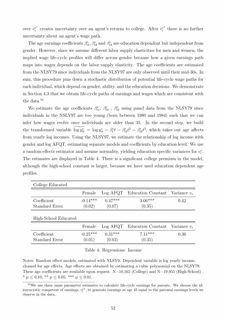
over ve⇤
icreates uncertainty over an agent’s returns to college. After v
e⇤
ithere is no further
uncertainty about an agent’s wage path.The age earnings coefficients �e
t1, �e
t2 and �e
t3 are education dependent but independent fromgender. However, since we assume different labor supply elasticities for men and women, theimplied wage life-cycle profiles will differ across gender because how a given earnings pathmaps into wages depends on the labor supply elasticity. The age coefficients are estimatedfrom the NLSY79 since individuals from the NLSY97 are only observed until their mid-30s. Insum, this procedure pins down a stochastic distribution of potential life-cycle wage paths foreach individual, which depend on gender, ability, and the education decisions. We demonstratein Section 4.3 that we obtain life-cycle paths of earnings and wages which are consistent withthe data.54
We estimate the age coefficients �e
t1, �e
t2 , �e
t3 using panel data from the NLSY79 sinceindividuals in the NSLY97 are too young (born between 1980 and 1984) such that we caninfer how wages evolve once individuals are older than 35. In the second step, we buildthe transformed variable log ye
it= log ye
it� �
e
tt � �
e
t2t2 � �
e
t3t3, which takes out age affects
from yearly log incomes. Using the NLSY97, we estimate the relationship of log income withgender and log AFQT, estimating separate models and coefficients by education level. We usea random-effects estimator and assume normality, yielding education specific variances for ve
i.
The estimates are displayed in Table 4. There is a significant college premium in the model,although the high-school constant is larger, because we have used education dependent ageprofiles.
College Educated
Female Log AFQT Education Constant Variance vi
Coefficient -0.14*** 0.47*** 3.06*** 0.42Standard Error (0.02) (0.07) (0.35)
High-School Educated
Female Log AFQT Education Constant Variance vi
Coefficient -0.25*** 0.31*** 7.11*** 0.36Standard Error (0.01) (0.03) (0.35)
Table 4: Regressions: Income
Notes: Random effect models, estimated with NLSY9. Dependent variable is log yearly income,cleaned for age effects. Age effects are obtained by estimating a cubic polynomial on the NLSY79.These age coefficients are available upon request. N=10,165 (College) and N=19,955 (High-School) .* p 0.10, ** p 0.05, *** p 0.01.
54We use these same parameter estimates to calculate life-cycle earnings for parents. We choose the id-iosyncratic competent of earnings, ve⇤
i, to generate earnings at age 45 equal to the parental earnings levels we
observe in the data.
52

Next, we explain how to go from the estimated income to the wage profiles. The reasonwhy we do not estimate wage profiles directly is that we append Pareto tails to the income dis-tribution on which more reliable information is available. Top incomes are underrepresentedin the NLSY as in most survey data sets. Following common practice in the optimal tax liter-ature (Piketty and Saez, 2013), we therefore append Pareto tails to each income distribution,starting at incomes of $150,000. We set the shape parameter ↵ of the Pareto distribution to1.5 for all income distributions.
Next we describe the mapping from y to w as in Saez (2001). Given the utility function weassume with no income effects, in each year individuals solve a static labor supply problemwhere optimal labor supply in that year only depends on the current wage (which evolves overthe life-cycle) and marginal tax distortions. It is easy to show that the first-order conditionfor an individual facing a marginal tax rate schedule is
lnw =✏+ ⌧
1 + ✏ln y � 1
1 + ✏ln(� (1� ⌧)),
if the tax function is of the form T (y) = y � ⇢y1�⌧ . Using the estimates from the regression
model, we can express the wage for a given type (age, gender, ability, education) as at age t:
lnwit =✏+ ⌧
1 + ✏
⇣�es
0 + �e
✓log ✓i + �
e
tt+ �
e
t2t2 + �
e
t3t3 + v
e⇤
i
⌘� 1
1 + ✏ln(� (1� ⌧)).
B.4 Value Functions During College
Agents do not graduate and remain in college with probability�1� Pr
Grad
t(✓)�, which depends
on the agent’s ability level ✓. Further, we allow the interest rate the agent receives in collegeto vary by the agent’s assets (positive or negative) and by the agent’s parental income, toreflect features of the Stafford loan program.
VE,`
E
t
t
⇣X, I, at, "
`E
t
t
⌘= max
ct
[UE
⇣ct, `
E
t, X, "
`E
t
⌘+
���
1� PrGrad
t(✓)�E⇥V
E
t+1 (X, I, at+1, "t+t)⇤+ Pr
Grad
t(✓)E
⇥V
W
t+1 (X, e = G, at+1, wt+1)⇤
(17)
subject toct = `
E
t! + at (1 + r (at, I))� at+1 � FRegion + G (X, I)
andat+1 � a
E
t+1,
where V E
t+1 (X, I, at+1, "t+t) and "t+t are defined in the main body. The term⇥V
W
t+1 (X, e = G, at+1, wt+1)⇤
is the expected value of being a college graduate in the workforce in year t + 1, where theexpectation is taken over the permanent skill shock. We allow tuition, FRegion, to depend on
53
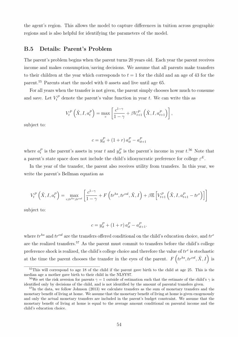
the agent’s region. This allows the model to capture differences in tuition across geographicregions and is also helpful for identifying the parameters of the model.
B.5 Details: Parent’s Problem
The parent’s problem begins when the parent turns 20 years old. Each year the parent receivesincome and makes consumption/saving decisions. We assume that all parents make transfersto their children at the year which corresponds to t = 1 for the child and an age of 43 for theparent.55 Parents start the model with 0 assets and live until age 65.
For all years when the transfer is not given, the parent simply chooses how much to consumeand save. Let V
P
tdenote the parent’s value function in year t. We can write this as
VP
t
⇣X, I, a
P
t
⌘= max
c
c1��
1� �+ �V
P
t+1
⇣X, I, a
P
t+1
⌘�,
subject to:
c = yP
it+ (1 + r) aP
it� a
P
it+1
where aP
tis the parent’s assets in year t and y
P
itis the parent’s income in year t.56 Note that
a parent’s state space does not include the child’s idiosyncratic preference for college "E.
In the year of the transfer, the parent also receives utility from transfers. In this year, wewrite the parent’s Bellman equation as
VP
t
⇣X, I, a
P
t
⌘= max
c,trhs,trcol
c1��
1� �+ F
⇣tr
hs, tr
col, X, I
⌘+ �E
hV
P
t+1
⇣X, I, a
P
t+1 � tre
⌘i�
subject to:
c = yP
it+ (1 + r) aP
it� a
P
it+1.
where trhs and trcol are the transfers offered conditional on the child’s education choice, and tr
e
are the realized transfers.57 As the parent must commit to transfers before the child’s collegepreference shock is realized, the child’s college choice and therefore the value of tre is stochasticat the time the parent chooses the transfer in the eyes of the parent. F
⇣tr
hs, tr
col, X, I
⌘is
55This will correspond to age 18 of the child if the parent gave birth to the child at age 25. This is themedian age a mother gave birth to their child in the NLSY97.
56We set the risk aversion for parents � = 1 outside of estimation such that the estimate of the child’s � isidentified only by decisions of the child, and is not identified by the amount of parental transfers given.
57In the data, we follow Johnson (2013) we calculate transfers as the sum of monetary transfers and themonetary benefit of living at home. We assume that the monetary benefit of living at home is given exogenouslyand only the actual monetary transfers are included in the parent’s budget constraint. We assume that themonetary benefit of living at home is equal to the average amount conditional on parental income and thechild’s education choice.
54
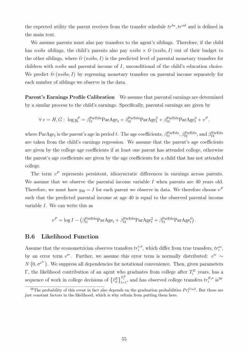
the expected utility the parent receives from the transfer schedule trhs, tr
col and is defined inthe main text.
We assume parents must also pay transfers to the agent’s siblings. Therefore, if the childhas nsibs siblings, the child’s parents also pay nsibs ⇥ tr (nsibs, I) out of their budget tothe other siblings, where tr (nsibs, I) is the predicted level of parental monetary transfers forchildren with nsibs and parental income of I, unconditional of the child’s education choice.We predict tr (nsibs, I) by regressing monetary transfers on parental income separately foreach number of siblings we observe in the data.
Parent’s Earnings Profile Calibration We assume that parental earnings are determinedby a similar process to the child’s earnings. Specifically, parental earnings are given by
8 e = H,G : log yPt= �
ParEdut1 ParAge
t+ �
ParEdut2 ParAge2
t+ �
ParEdut3 ParAge3
t+ v
P.
where ParAgetis the parent’s age in period t. The age coefficients, �ParEdu
t1 , �ParEdut2 , and �
ParEdut3
are taken from the child’s earnings regression. We assume that the parent’s age coefficientsare given by the college age coefficients if at least one parent has attended college, otherwisethe parent’s age coefficients are given by the age coefficients for a child that has not attendedcollege.
The term vP represents persistent, idiosyncratic differences in earnings across parents.
We assume that we observe the parental income variable I when parents are 40 years old.Therefore, we must have y40 = I for each parent we observe in data. We therefore choose v
P
such that the predicted parental income at age 40 is equal to the observed parental incomevariable I. We can write this as
vP = log I �
��
ParEdut1 ParAge
t+ �
ParEdut2 ParAge2
t+ �
ParEdut3 ParAge3
t
�.
B.6 Likelihood Function
Assume that the econometrician observes transfers tre,oi
, which differ from true transfers, tre?i
,by an error term e
tr. Further, we assume this error term is normally distributed: etr ⇠
N�0, �e
tr�. We suppress all dependencies for notational convenience. Then, given parameters
�, the likelihood contribution of an agent who graduates from college after TE
iyears, has a
sequence of work in college decisions of�`E
it
TE
i
t=1, and has observed college transfers tr
E,o
iis58
58The probability of this event in fact also depends on the graduation probabilities PrGrad
t. But these are
just constant factors in the likelihood, which is why refrain from putting them here.
55
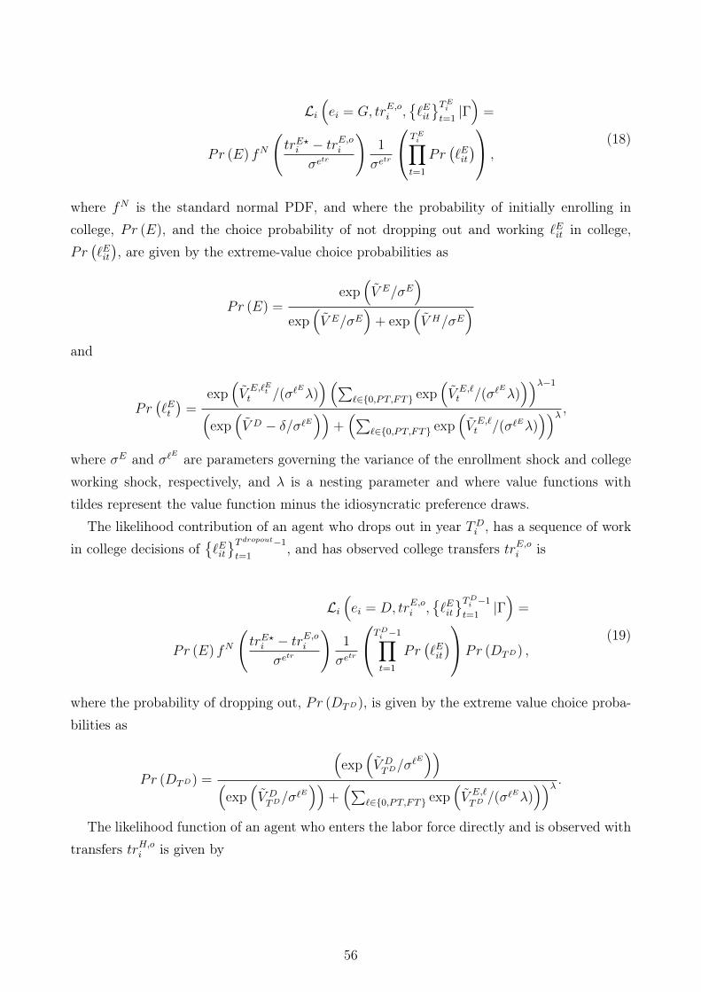
Li
⇣ei = G, tr
E,o
i,�`E
it
TE
i
t=1|�⌘=
Pr (E) fN
tr
E?
i� tr
E,o
i
�etr
!1
�etr
0
@T
E
iY
t=1
Pr�`E
it
�1
A ,
(18)
where fN is the standard normal PDF, and where the probability of initially enrolling in
college, Pr (E), and the choice probability of not dropping out and working `E
itin college,
Pr�`E
it
�, are given by the extreme-value choice probabilities as
Pr (E) =exp
⇣V
E/�
E
⌘
exp⇣V E/�E
⌘+ exp
⇣V H/�E
⌘
and
Pr�`E
t
�=
exp⇣V
E,`E
t
t /(�`E
�)⌘⇣P
`2{0,PT,FT} exp⇣V
E,`
t /(�`E
�)⌘⌘��1
⇣exp
⇣V D � �/�`E
⌘⌘+⇣P
`2{0,PT,FT} exp⇣V
E,`
t /(�`E�)⌘⌘� ,
where �E and �
`E are parameters governing the variance of the enrollment shock and college
working shock, respectively, and � is a nesting parameter and where value functions withtildes represent the value function minus the idiosyncratic preference draws.
The likelihood contribution of an agent who drops out in year TD
i, has a sequence of work
in college decisions of�`E
it
T dropout�1
t=1, and has observed college transfers tr
E,o
iis
Li
⇣ei = D, tr
E,o
i,�`E
it
TD
i�1
t=1|�⌘=
Pr (E) fN
tr
E?
i� tr
E,o
i
�etr
!1
�etr
0
@T
D
i�1Y
t=1
Pr�`E
it
�1
APr (DTD) ,(19)
where the probability of dropping out, Pr (DTD), is given by the extreme value choice proba-bilities as
Pr (DTD) =
⇣exp
⇣V
D
TD/�`E
⌘⌘
⇣exp
⇣V
D
TD/�`E
⌘⌘+⇣P
`2{0,PT,FT} exp⇣V
E,`
TD /(�`E�)⌘⌘� .
The likelihood function of an agent who enters the labor force directly and is observed withtransfers tr
H,o
iis given by
56

Li
⇣ei = H, tr
H,o
i|�⌘= (1� Pr (E)) fN
tr
H?
i� tr
H,o
i
�etr
!1
�etr. (20)
We therefore choose the parameters � to maximize the log likelihood:
max�
X
i
logLi (·|�) .
B.7 Identification
B.7.1 Identification of Main Parameters
The parameter � and the parameter governing the variance of the college-enrollment preferenceshock, �E, play crucial roles in our analysis as they determine the extent to which increasingfinancial aid affects the college enrollment decision. Higher values of �
E and lower valuesof � imply a smaller elasticity of enrollment with respect to increases in financial aid. Theseparameters are jointly identified by the relationship between enrollment and parental income ofotherwise similar individuals. Enrolling in college will generally imply lower net income whileenrolled in college and higher income later in life. To the extent that borrowing constraintsare effective and that parental transfers are increasing in parental income, children from lower-income backgrounds will not be able to smooth consumption and therefore will have lowerconsumption in their early life. The parameter � determines the cost of not being able tosmooth consumption early in life. A high value of � therefore implies low college enrollmentfor individuals close to the borrowing constraint.
Furthermore, exclusion restrictions in the grant function help us to identify the elasticityof college going with respect to financial aid. Tuition varies by region but region does notenter the earnings function or utility function. Therefore, similar to Heckman et al. (1998),variation in tuition levels creates variation in the value of college enrollment which helps us toidentify � and �
E. In Section B.7.2 we use a simple example to build intuition on how thesetwo parameters are separately identified.
Additionally, the extent to which poor students are more likely to work than rich studentswill be governed by �; this tells us how much more students who are close to the borrowingconstraint are willing to work relative to those who are not. As such, we can identify � bycomparing the labor supply decisions of poor students with those from rich students.
The psychic cost of college, X , is identified by different rates of attending college byability, gender, and parental education, after controlling for differences in utility coming fromconsumption and differences in future earnings. The parameters governing the value of workingin college, ⇣, �
`E , and �, are jointly identified by variation in college labor supply choices
across agents and across periods. Specifically, the parameter vector ⇣ is identified by different
57

rates of working in college after controlling for differences in utility coming from consumptionand differences in future earnings. The parameter governing the variance of the labor supplyshock, �`
E , is identified by variation in the timing of working in college decisions. For example,suppose that �
`E
= 0. Then the labor supply decisions of identical agents would be exactlythe same in each period. A larger �
`E implies more variation in the labor supply choices of
identical agents and across periods. The nesting parameter �, is identified by the substitutionpatterns across labor supply decisions and dropping out. The warm-glow parameters, � andcb, are identified by the relationship between parental income and parental transfers. A largervalue of � increases the derivative of parental transfers on parental income. Decreasing cb
increases the level of transfers overall. Warm-glow utility only depends on the amount oftransfers given, not on other things that may enter the child’s problem (i.e., ability, tuition,number of siblings). The degree to which parental transfers respond to different children’scharacteristics will instead be determined by the strength of the altruism motive. Therefore,any differences in parental transfers across student characteristics will identify !. For example,if students who face higher tuition levels generally receive higher parental transfers, this willidentify ! and give us a sense of how much we expect parental transfers to be crowded outby financial aid. Parents’ paternalism parameters, ⇠0 and ⇠ParEd, are identified by the ratioof college parental transfers to high school parental transfers. A higher value of ⇠0 implieshigher transfers for children going to college relative to transfers for children entering the laborforce directly. Finally, the parameter governing the standard deviation of observed parentaltransfers, �e
tr , is identified by the variance in observed parental transfers of identical agents.
B.7.2 Identification in a Simplified Model
In this section we use a simple model to show how the parameter governing the the agents’risk aversion, �, is separately identified from the variance of the idiosyncratic taste for college�E.Consider a simple static model where agents make a discrete choice over options j, rep-
resenting schooling options. For an agent i, each option has an associated income Yij whichcould represent, for example, how much income an agent has left for consumption net of tuitioncosts. Let an agent’s choice specific utility be given by:
uij =c1��
ij
1� �+ j + �"ij
where j is a parameter that is common to all agents who choose option j and "ij is an extremevalue-type I preference parameter. Collectively, we can think of � (j + "ij) as the psychiccost of option j. As this is a static model, let cij = Yij.
Note that (1� �) shows up in two places in the utility function. First it shows up asthe denominator of c
1��
ij
1��and therefore scales utility from consumption. This scaling factor
58

alone is not separately identified from the variance of the error term �. However, (1� �) alsoshows up as the exponent on consumption, and therefore dictates the curvature of utility fromconsumption. This is crucial for separately identifying � from �. Essentially if � is large (and(1��) small), then agents with lower levels of income will behave differently than agents withhigher levels of income.
Suppose we can divide agents i into several different “regions”. All agents in a given regionr face the same menu of incomes across options. We will therefore write all choice specificincomes as Yrj. Note that agents across regions all have same preferences but face differentincome levels, representing differences in tuition across regions, differences in wage income incollege, or differences in parental transfers.
The probability that an agent in region r chooses option j is given by:
Prj =
exp
✓Y
1��
rj
�(1��) +j
�
◆
Pj0 exp
✓Y
1��
rj0
�(1��) +j0
�
◆
We can then write the log ratio of choice probabilities of choosing option j over k for agentsin region r:
logPrj
Prk
=1
�
" Y
1��
rj
(1� �)+ j
!�✓
Y1��
rk
(1� �)+ k
◆#(21)
Now consider the difference in this log ratio between agents in region r and agents in regionr:
logPrj
Prk
� logPrj
Prk
=1
(1� �) �
⇥�Y
1��
rj� Y
1��
rk
���Y
1��
rj� Y
1��
rk
�⇤(22)
Before completing the proof, we consider a simple example here to build intuition. Supposeagents in region r are poorer by a positive amount ⌧ for both options, relative to agentsin region r. That is: Yrj = Yrj � ⌧ and Yrk = Yrk � ⌧ . Then � = 0 would imply thatlog Prj
Prk
� log Prj
Prk
= 0— the ratio of choice probabilities in the poor region is equal to the ratioin the rich region. Larger � implies that the poorer region will choose the relatively higherincome option more relative to the richer region.
Consider now a third region, r. We now also have
logPrj
Prk
� logPrj
Prk
=1
(1� �) �
⇥�Y
1��
rj� Y
1��
rk
���Y
1��
rj� Y
1��
rk
�⇤(23)
combined with 22, this gives us two equations and two unknowns. Further, taking the ratioof 22 and 23 yields:
log Prj
Prk
� log Prj
Prk
log Prj
Prk
� log Prj
Prk
=
�Y
1��
rj� Y
1��
rk
���Y
1��
rj� Y
1��
rk
��Y
1��
rj� Y
1��
rk
���Y
1��
rj� Y
1��
rk
�
59

Table 5: Maximum Likelihood estimates
Estimate Standard Error
College Utility: UE (c, `) = c
1��
1��� ✓,d � ⇣
`E
+ "`E
it
Curvature of Utility � 1.9 0.0057No work ⇣
0 0 (Normalization)Part time ⇣
1 0.057 3.6?Full time ⇣
2 0.18 4.1?Standard Deviation of Enrollment Shock �
{E} 7.8? .069?Dropout cost � 1.2 1.7?
Standard Deviation of Working Shock �{`E} 0.40 .0078?
Nesting Parameter � 0.59 0.38?
Psychic Cost: ✓,d = 0 + ✓ log (✓i) + femI (s = female) + ParEdParEdui
Constant 0 0.44 0.15?Ability Interaction ✓ -8.3? 0.014?Female Dummy fem -0.083? 0.00075?Parental Education ParEd -1.7? 0.0049?
Parental Utility from Transfers:
F�tr
H, tr
E,⌦i
�= !EV
�⌦i|trH , tr
E�
| {z }Altruism
+E
2
664(⇠0 + ⇠ParEdParEdui)1E
| {z }Paternalism
+�(cb + tr
e)1��
1� �| {z }Warm Glow
3
775
Altruiusm ! 3.0 0.021Prestige Constant ⇠0 0.27 0.0017Parent’s Education Interaction ⇠ParEd 0.69? 0.00024?Warm Glow Strength � 0.09 0.0016Warm Glow Level cb -3.4 ?? 0.059??
? we display 10,000 times the parameter value.?? we display the parameter value divided by 10,000.
which identifies �. � is therefore identified by 22. Finally, we must normalize one of thej = 0. Then all of the j terms are identified by 21.
B.8 ML Estimates
The parameter estimates are contained in Table 5.
B.9 Graduation Rates and Enrollment by Gender
Figure 11 shows the college graduation rates as a function of parental income and ability inthe model and in the data. The model is able to replicate these moments well.
Figure 12(a) shows the college enrollment rates for male and female students as a functionof parental income in the model and in the data. Figure 12(b) shows the college enrollmentrates for male and female students as a function of ability in the model and in the data. Wecan see that the model is able to replicate these moments quite well.
60

(a) Graduation Rates and Parental Income (b) Graduation Rates and AFQT
Figure 11: Graduation and Enrollment Rates
Notes: The solid (red) line shows simulated enrollment shares by parental income and AFQTpercentile. This is compared to the dashed (black) line which shows the shares in the data.
B.10 Earnings Profiles Model
Figure 13 shows the simulated average for college graduates and high school graduates as afunction of age.
B.11 Untargeted Moments
Responsiveness of Enrollment to Grant Increases. Many papers have analyzed theimpact of increases in grants or decreases in tuition on college enrollment. Deming andDynarski (2009) survey the literature. The estimated impact of a $1,000 increase in yearlygrants (or a respective reduction in tuition) on enrollment ranges from 1 to 6 percentage points,depending on the policy reform and research design. A more recent study by Castlemanand Long (2016) looks at the impact of grants targeted to low-income children. Applying aregression-discontinuity design for need-based financial aid in Florida (Florida Student AccessGrant), they find that a $1,000 increase in yearly grants for children with parental incomearound $30,000 increases enrollment by 2.5 percentage points.
Simulating a $1,000 increase in financial aid for all individuals in our model leads to a 1.69percentage point increase in overall enrollment rates and a 2.06 percentage point increase forstudents near the studied discontinuity in Castleman and Long (2016). Overall, our simulatedelasticities are fairly consistent with these reduced-form estimates. This gives us confidencein our maximum likelihood estimates, especially given that these reduced form estimates werenot targeted in estimation.
Importance of Parental Income. A well-known empirical fact is that individuals withhigher parental income are more likely to receive a college degree (see also Figure 2). However,
61

(a) Enrollment Rates and Parental Income (b) Enrollment Rates and AFQT
Figure 12: Graduation and Enrollment Rates by Gender
Notes: The panel on the left shows the relationship between enrollment rates and parental incomein the model and in the data for females and males. The panel on the right shows the relationshipbetween enrollment rates and ability in the model and in the data for females and males.
Figure 13: College and High School Graduate Earnings Profiles.
it is not obvious whether this is primarily driven by parental income itself or by variablescorrelated with parental income and college graduation. Using income tax data and a researchdesign exploiting parental layoffs, Hilger (2016) finds that a $1,000 increase in parental incomeleads to an increase in college enrollment of 0.43 percentage points. To test our model, weincreased parental income for each individual by $1,000 and obtained increases in collegeenrollment by 0.18 percentage points. Our model predicts a moderate direct effect of parentalincome, smaller but in line with Hilger (2016).
Returns for Marginal Students. We find a return to one year of schooling of 12.1% formarginal students. This reflects that marginal students are of lower ability on average thaninframarginal students and is also in line with Oreopoulos and Petronijevic (2013). A clean wayto infer returns for marginal students is found in Zimmerman (2014). In his study, studentsare marginal with respect to academic ability, measured by a GPA admission cutoff. He finds
62

that these students have earnings 22% higher than those just below the cutoff, when earningsare measured 8 to 14 years after high school graduation. We perform a similar simulation andmake use of the fact that the NLSY also provides GPA data. In fact, our model gives a returnto college of 26.3%, measured 8 to 14 years after high school graduation, for students with aGPA in this neighborhood.59
C Additional Results
C.1 Marginal and Inframarginals Evaluated at Current Financial
Aid Levels
In Section 6.1, we plotted the share of marginal enrollees and inframarginal enrollees at a flatfinancial schedule for a number of model specifications. In this section, we repeat this exercisebut plot the share of marginal enrollees and inframarginal enrollees at the current financialaid schedule.
The results are very similar to those presented in Section 6.1. The relationship betweenparental income and share of inframarginal students has become weaker (and eventually be-comes negative), reflecting that the current financial aid schedule is decreasing in parentalincome, see Figure 14(a). Further, children with high income parents are more likely to bemarginal with respect to financial aid relative to graph is in Section 6.1, again reflecting thatthey receive less financial aid then children with low income parents, see Figure 14(b).
C.2 An Alternative Decomposition
In Section 6.1, we perform a model-based decomposition exercise to better understand whichdrive the optimal progressivity result. In this appendix, we perform a similar decompositionbut alter the order in which we change various components to the model. In particular, we firstremove the relationship between parental income and parental transfers, before proceeding toremove the relation between parental income and ability and the relation between parentaleducation and the psychic costs of college. As before, all changes to the model specificationare cumulative.
We first analyze the determinants of the positive relation between college enrollment andparental income in Figure 15(a) and the negative relationship between share of marginal stu-dents and parental income in Figure 15(a). The simulated relationships at a flat financial aid
59Finally, we do not account for differing rates of unemployment and disability insurance rates. Bothnumbers are typically found to be only half as large for college graduates (see Oreopoulos and Petronijevic(2013) for unemployment and Laun and Wallenius (2016) for disability insurance). Further, the fiscal costsof Medicare are likely to be much lower for individuals with a college degree. Lastly, we assume that allindividuals work until 65 not taking into account that college graduates on average work longer (Laun andWallenius, 2016). These facts would generally strengthen the case for an increase in college subsidies.
63

(a) Inframarginal Enrollees (b) Marginal Students
Figure 14: Model-Based Decomposition for Marginal and Inframarginal Students at CurrentGrant Schedule
Notes: We plot the share of college enrollees and marginal college enrollees given the current US aidschedule for different model specifications. The solid red line represent the baseline model. For thedashed black line we simulate a model version for which we remove the correlation between abilityand parental income. For the dashed-dotted blue line we simulate a model version for which weadditionally remove the correlation between the psychic costs and parental education. For thedotted pink line we simulate a model version for which additionally removes labor market riskiness;i.e. education decisions are made with no uncertainty about future wages. For the turquoise linewith crosses we simulate a model version for which we set parental transfers to the mean parentaltransfers in the data, conditional on education.
schedule are shown in the solid lines in the two figures. In this baseline case, college enroll-ment rates are strongly increasing in parental income while the share of marginal students arestrongly decreasing in parental income. Next, in the turquoise lines, we set parental transfersexogenously to the mean levels for enrollees and non-enrollees and assume no families areeligible for subsidized Stafford loans. From Figure 15(a) we can see that the positive rela-tion between college enrollment and parental income weakens slightly. The relation betweenparental income and share of marginal enrollees, however, flattens completely. The blackdotted line and the blue dash-dotted line show the cases in which we remove the correlationbetween parental income and ability and in which we remove the relation between parentaleducation and psychic costs, respectively. After removing these two factors there is no inter-esting heterogeneity between parental income groups. Removing these two relationships bothweak the relationship between parental income and enrollment. In both these simulations, thegradient between parental income and share of marginal students remains flat.
We now simulate the respective optimal financial aid schedule under each model specifica-tion in Figure 16. When we remove the relationship between parental income and parentaltransfers (the turquoise line in Figure 16), the optimal financial aid schedule flattens. Thisflattening of the optimal schedule occurs because the relationship between parental income
64

(a) Inframarginal Graduates (b) Marginal Students
Figure 15: Alternative Model-Based Decomposition for Marginal and Inframarginal Studentsat Flat Grant Schedule
Notes: We plot the share of college enrollees and marginal college enrollees given a flat financial aidschedule for different model specifications. The solid red line represent the full model. For theturquoise line with crosses we simulate a model version for which set parental transfers to the meanparental transfers in the data, conditional on education. For the dashed black line we simulate amodel version for which we remove the correlation between ability and parental income. For thedashed-dotted blue line we simulate a model version for which we additionally remove thecorrelation between the psychic costs and parental education.
and share of marginal enrollees is flat. However, there optimal aid is still positive—rangingfrom above $6,500 for the poorest families to below $4,500 for the wealtheat families. Theoptimal aid schedule is progressive because high income children are still much more likely in-framarginal. When we remove the positive ability-income correlation (the black dashed line)and the relationship between parental education and psychic costs we flatten the relation-ship between parental income and share of inframarginal students. The optimal aid scheduleflattens as a result.
C.3 Decomposition with Removal of Borrowing Constraints
In Figures 17(a) and 17(b), we perform the same decomposition we performed in Section6.1 but additionally remove borrowing constraints before equalizing parental transfers. Weadditionally assume that no families are eligible for subsidized Stafford loans throughoutthe decomposition. Figure 18 shows the resulting optimal financial aid under each modelspecification.
As before, the red line shows the baseline case, the black dotted line shows the case wherewe remove the ability correlation, the blue dash-dotted line shows the case where we removethe correlation between psychic cost of parental education, and the dotted pink line showthe case with no labor market uncertainty. These lines tell essentially the same story as thedecomposition in Section 6.1.
65
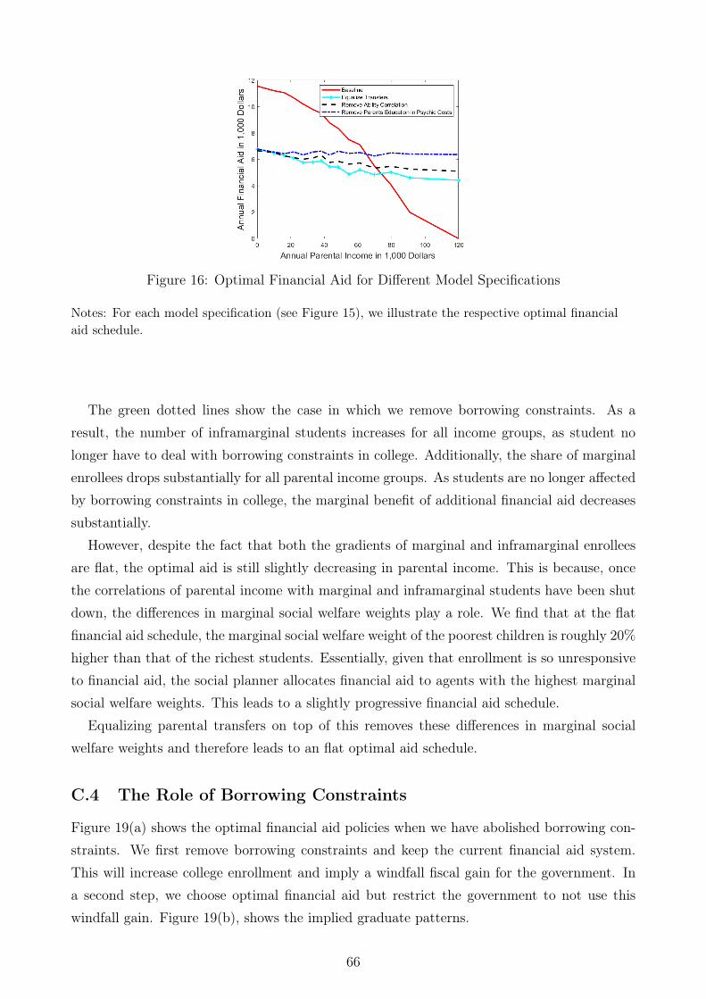
Figure 16: Optimal Financial Aid for Different Model Specifications
Notes: For each model specification (see Figure 15), we illustrate the respective optimal financialaid schedule.
The green dotted lines show the case in which we remove borrowing constraints. As aresult, the number of inframarginal students increases for all income groups, as student nolonger have to deal with borrowing constraints in college. Additionally, the share of marginalenrollees drops substantially for all parental income groups. As students are no longer affectedby borrowing constraints in college, the marginal benefit of additional financial aid decreasessubstantially.
However, despite the fact that both the gradients of marginal and inframarginal enrolleesare flat, the optimal aid is still slightly decreasing in parental income. This is because, oncethe correlations of parental income with marginal and inframarginal students have been shutdown, the differences in marginal social welfare weights play a role. We find that at the flatfinancial aid schedule, the marginal social welfare weight of the poorest children is roughly 20%higher than that of the richest students. Essentially, given that enrollment is so unresponsiveto financial aid, the social planner allocates financial aid to agents with the highest marginalsocial welfare weights. This leads to a slightly progressive financial aid schedule.
Equalizing parental transfers on top of this removes these differences in marginal socialwelfare weights and therefore leads to an flat optimal aid schedule.
C.4 The Role of Borrowing Constraints
Figure 19(a) shows the optimal financial aid policies when we have abolished borrowing con-straints. We first remove borrowing constraints and keep the current financial aid system.This will increase college enrollment and imply a windfall fiscal gain for the government. Ina second step, we choose optimal financial aid but restrict the government to not use thiswindfall gain. Figure 19(b), shows the implied graduate patterns.
66
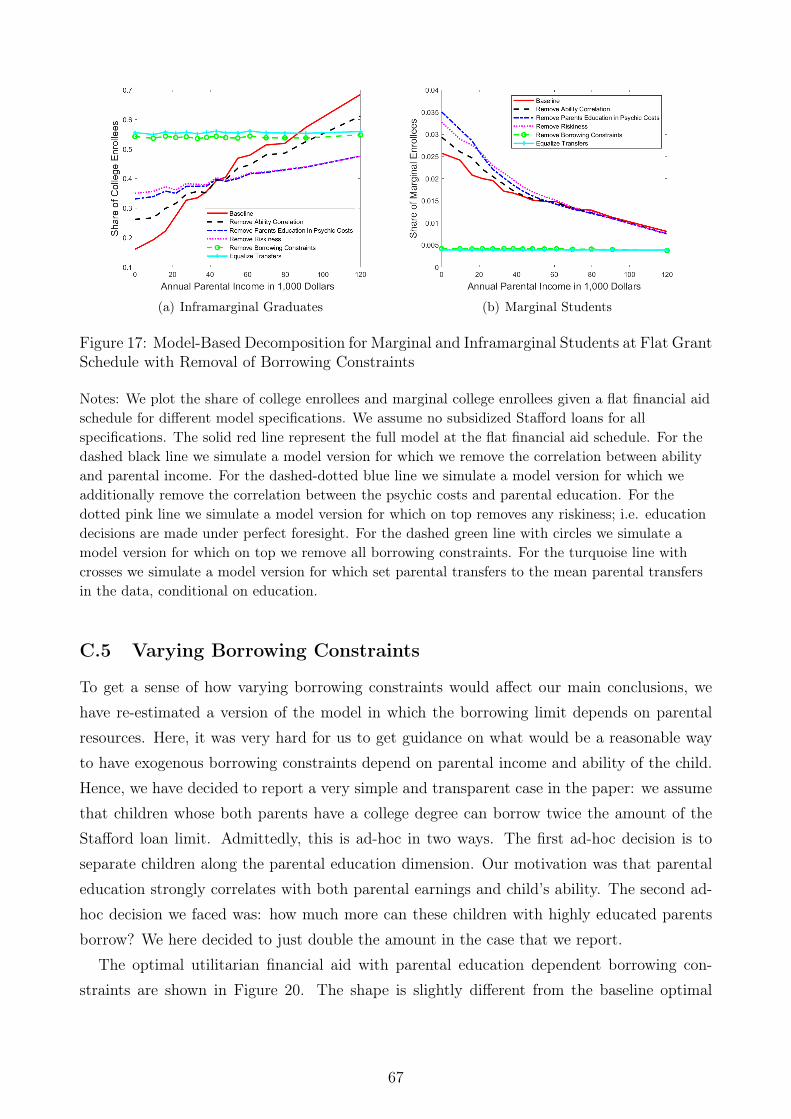
(a) Inframarginal Graduates (b) Marginal Students
Figure 17: Model-Based Decomposition for Marginal and Inframarginal Students at Flat GrantSchedule with Removal of Borrowing Constraints
Notes: We plot the share of college enrollees and marginal college enrollees given a flat financial aidschedule for different model specifications. We assume no subsidized Stafford loans for allspecifications. The solid red line represent the full model at the flat financial aid schedule. For thedashed black line we simulate a model version for which we remove the correlation between abilityand parental income. For the dashed-dotted blue line we simulate a model version for which weadditionally remove the correlation between the psychic costs and parental education. For thedotted pink line we simulate a model version for which on top removes any riskiness; i.e. educationdecisions are made under perfect foresight. For the dashed green line with circles we simulate amodel version for which on top we remove all borrowing constraints. For the turquoise line withcrosses we simulate a model version for which set parental transfers to the mean parental transfersin the data, conditional on education.
C.5 Varying Borrowing Constraints
To get a sense of how varying borrowing constraints would affect our main conclusions, wehave re-estimated a version of the model in which the borrowing limit depends on parentalresources. Here, it was very hard for us to get guidance on what would be a reasonable wayto have exogenous borrowing constraints depend on parental income and ability of the child.Hence, we have decided to report a very simple and transparent case in the paper: we assumethat children whose both parents have a college degree can borrow twice the amount of theStafford loan limit. Admittedly, this is ad-hoc in two ways. The first ad-hoc decision is toseparate children along the parental education dimension. Our motivation was that parentaleducation strongly correlates with both parental earnings and child’s ability. The second ad-hoc decision we faced was: how much more can these children with highly educated parentsborrow? We here decided to just double the amount in the case that we report.
The optimal utilitarian financial aid with parental education dependent borrowing con-straints are shown in Figure 20. The shape is slightly different from the baseline optimal
67

Figure 18: Optimal Financial Aid for Different Model Specifications
Notes: For each model specification (see Figure 17), we illustrate the respective optimal financialaid schedule.
schedule, as changes in the borrowing constraints lead to changes share of marginal students.60
However, the optimal financial aid is still highly progressive.
C.6 Details: Endogenous Ability
We assume that initial ability ✓0 is distributed as:
ln ✓0 = �0 + �1 ln I + u
where u is normally distributed. We choose �0, �1, and the variance of u to match the meanand variance of log childhood ability and covariance of log childhood ability and log parentalincome from Agostinelli and Wiswall (2016).
We need to calibrate the parameters of the childhood ability production function:
1. A- TFP of parental production function.
2. �1 - weight on initial ability
3. �2 - weight on parental investment
4. �3 - interaction term
5. �◆ - variance of ◆.
60As we have shown earlier, relaxing borrowing constraints for all students reduces the progressivity of theoptimal aid schedule. That force is still present here, as some low income students have two college educatedparents. However, this force is partially muted by the fact that parental education is increasing in parentalincome. As such, the optimal aid schedule here is more progressive than the case with relaxed borrowing con-straints for all individuals, but slightly less progressive than the baseline case with equal borrowing constraintsfor all students.
68
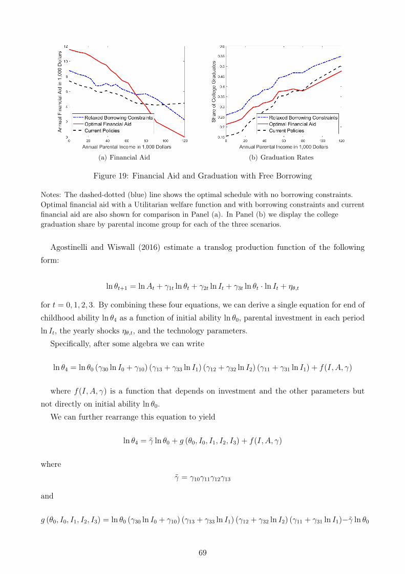
(a) Financial Aid (b) Graduation Rates
Figure 19: Financial Aid and Graduation with Free Borrowing
Notes: The dashed-dotted (blue) line shows the optimal schedule with no borrowing constraints.Optimal financial aid with a Utilitarian welfare function and with borrowing constraints and currentfinancial aid are also shown for comparison in Panel (a). In Panel (b) we display the collegegraduation share by parental income group for each of the three scenarios.
Agostinelli and Wiswall (2016) estimate a translog production function of the followingform:
ln ✓t+1 = lnAt + �1t ln ✓t + �2t ln It + �3t ln ✓t · ln It + ⌘✓,t
for t = 0, 1, 2, 3. By combining these four equations, we can derive a single equation for end ofchildhood ability ln ✓4 as a function of initial ability ln ✓0, parental investment in each periodln It, the yearly shocks ⌘✓,t, and the technology parameters.
Specifically, after some algebra we can write
ln ✓4 = ln ✓0 (�30 ln I0 + �10) (�13 + �33 ln I1) (�12 + �32 ln I2) (�11 + �31 ln I1) + f(I, A, �)
where f(I, A, �) is a function that depends on investment and the other parameters butnot directly on initial ability ln ✓0.
We can further rearrange this equation to yield
ln ✓4 = � ln ✓0 + g (✓0, I0, I1, I2, I3) + f(I, A, �)
where� = �10�11�12�13
and
g (✓0, I0, I1, I2, I3) = ln ✓0 (�30 ln I0 + �10) (�13 + �33 ln I1) (�12 + �32 ln I2) (�11 + �31 ln I1)�� ln ✓0
69
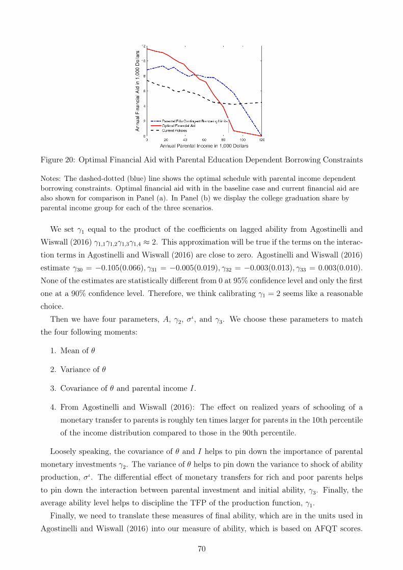
Figure 20: Optimal Financial Aid with Parental Education Dependent Borrowing Constraints
Notes: The dashed-dotted (blue) line shows the optimal schedule with parental income dependentborrowing constraints. Optimal financial aid with in the baseline case and current financial aid arealso shown for comparison in Panel (a). In Panel (b) we display the college graduation share byparental income group for each of the three scenarios.
We set �1 equal to the product of the coefficients on lagged ability from Agostinelli andWiswall (2016) �1,1�1,2�1,3�1,4 ⇡ 2. This approximation will be true if the terms on the interac-tion terms in Agostinelli and Wiswall (2016) are close to zero. Agostinelli and Wiswall (2016)estimate �30 = �0.105(0.066), �31 = �0.005(0.019), �32 = �0.003(0.013), �33 = 0.003(0.010).None of the estimates are statistically different from 0 at 95% confidence level and only the firstone at a 90% confidence level. Therefore, we think calibrating �1 = 2 seems like a reasonablechoice.
Then we have four parameters, A, �2, �◆, and �3. We choose these parameters to matchthe four following moments:
1. Mean of ✓
2. Variance of ✓
3. Covariance of ✓ and parental income I.
4. From Agostinelli and Wiswall (2016): The effect on realized years of schooling of amonetary transfer to parents is roughly ten times larger for parents in the 10th percentileof the income distribution compared to those in the 90th percentile.
Loosely speaking, the covariance of ✓ and I helps to pin down the importance of parentalmonetary investments �2. The variance of ✓ helps to pin down the variance to shock of abilityproduction, �◆. The differential effect of monetary transfers for rich and poor parents helpsto pin down the interaction between parental investment and initial ability, �3. Finally, theaverage ability level helps to discipline the TFP of the production function, �1.
Finally, we need to translate these measures of final ability, which are in the units used inAgostinelli and Wiswall (2016) into our measure of ability, which is based on AFQT scores.
70

Let ✓ represent end of childhood ability as measured in the units used in Agostinelli andWiswall (2016). We assume that our measures of ability ✓ is a linear projection of this logskill measure
✓ = ↵0 + ↵1 ln ✓
where we choose ↵1 and ↵0 to match the mean and variance of our AFQT measure. Therefore,when we simulate the model, we first simulate childhood ability in the units used in Agostinelliand Wiswall (2016). Then we translate the measures of ability in Agostinelli and Wiswall(2016) to the ability measures we use in this paper.
Changes in Childhood Ability Figure 21 shows the change in the relationship betweenparental income and ability as a result of switching from the current financial aid systemto the optimal system with endogenous ability. Ability is measured in percentiles of AFQTscores where percentiles are evaluated at their current levels. We can see that switching tothe optimal aid schedule leads to substantial increases in child ability, especially for childrenin the lower end of the parental income distribution.
Figure 21: Ability Levels with Endogenous AbilityNotes: This figure shows the relationship between parental income and ability in the optimal systemwith endogenous ability and under the current financial aid system. Ability is measured in percentilesof the AFQT distribution before financial aid is re-optimized.
C.7 Endogenous Ability with Parental Borrowing Constraints
One issue with the preceding analysis is that we have assumed that parents do not faceborrowing constraints. Poor parents may be borrowing constrained while their children areyoung and therefore may not be able to increase investment in their children in response tochanges in financial aid. To explore how borrowing constraints would affect the optimal policy,we assume that P% of parents without a college education cannot increase their investment intheir children while the remainder of parents may choose their investment level without this
71

constraint.61 The optimal policy for a range of values of P is displayed in Figure 22. We cansee that the optimal progressivity of the system decreases as we increase the percentage oflow-education families who are borrowing constrained. However, the optimal schedule remainsmore progressive than the current schedule in all cases.
(a) Financial Aid (b) Graduation Rates
(c) Ability Levels
Figure 22: Financial Aid, Graduation and Ability Levels with Endogenous Ability andParental Borrowing ConstraintsNotes: In Panel (a), each line shows the optimal financial aid with endogenous ability when P percentof low-education parents are borrowing constrained and therefore cannot adjust their child’s ability inresponse to changes in financial aid. In Panel (b) we display the college graduation share for each ofthese scenarios. Panel (c) shows the relationship between parental income and ability in each scenario.Ability is measured in percentiles of the AFQT distribution before financial aid is re-optimized.
C.8 General Equilibrium Effects on Wages
Our analysis abstracted from general equilibrium effects on relative wages. Accounting forthese effects would imply that the effects of financial aid on enrollment might be mitigated in
61Caucutt and Lochner (2017) find that 20% of parents with a high school degree and young children areborrowing constrained. Of course, borrowing constraints will also affect the investment decisions of parentswho are not at the borrowing limit.
72
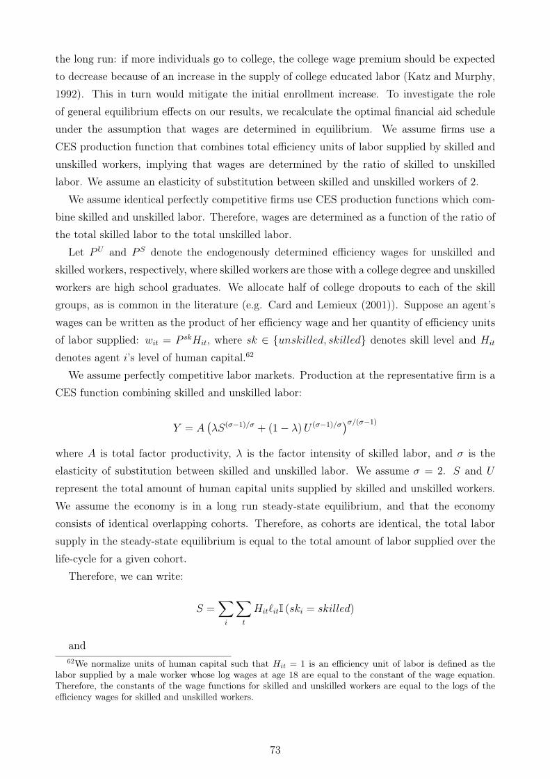
the long run: if more individuals go to college, the college wage premium should be expectedto decrease because of an increase in the supply of college educated labor (Katz and Murphy,1992). This in turn would mitigate the initial enrollment increase. To investigate the roleof general equilibrium effects on our results, we recalculate the optimal financial aid scheduleunder the assumption that wages are determined in equilibrium. We assume firms use aCES production function that combines total efficiency units of labor supplied by skilled andunskilled workers, implying that wages are determined by the ratio of skilled to unskilledlabor. We assume an elasticity of substitution between skilled and unskilled workers of 2.
We assume identical perfectly competitive firms use CES production functions which com-bine skilled and unskilled labor. Therefore, wages are determined as a function of the ratio ofthe total skilled labor to the total unskilled labor.
Let PU and P
S denote the endogenously determined efficiency wages for unskilled andskilled workers, respectively, where skilled workers are those with a college degree and unskilledworkers are high school graduates. We allocate half of college dropouts to each of the skillgroups, as is common in the literature (e.g. Card and Lemieux (2001)). Suppose an agent’swages can be written as the product of her efficiency wage and her quantity of efficiency unitsof labor supplied: wit = P
skHit, where sk 2 {unskilled, skilled} denotes skill level and Hit
denotes agent i’s level of human capital.62
We assume perfectly competitive labor markets. Production at the representative firm is aCES function combining skilled and unskilled labor:
Y = A��S
(��1)/� + (1� �)U (��1)/���/(��1)
where A is total factor productivity, � is the factor intensity of skilled labor, and � is theelasticity of substitution between skilled and unskilled labor. We assume � = 2. S and U
represent the total amount of human capital units supplied by skilled and unskilled workers.We assume the economy is in a long run steady-state equilibrium, and that the economyconsists of identical overlapping cohorts. Therefore, as cohorts are identical, the total laborsupply in the steady-state equilibrium is equal to the total amount of labor supplied over thelife-cycle for a given cohort.
Therefore, we can write:
S =X
i
X
t
Hit`itI (ski = skilled)
and62We normalize units of human capital such that Hit = 1 is an efficiency unit of labor is defined as the
labor supplied by a male worker whose log wages at age 18 are equal to the constant of the wage equation.Therefore, the constants of the wage functions for skilled and unskilled workers are equal to the logs of theefficiency wages for skilled and unskilled workers.
73

U =X
i
X
t
Hit`itI (ski = unskilled)
.Efficiency wages are given by the first order conditions of the firm’s profit maximization
problem:
PS = A
��S
(��1)/� + (1� �)U (��1)/��1/(��1)
�S�1/�
and
PU = A
��S
(��1)/� + (1� �)U (��1)/��1/(��1)
(1� �)U�1/�.
These two functions determine wages endogenously as functions of labor supply.The optimal financial aid schedule and graduation rates with general equilibrium wages are
shown in Figures 23(a) and 23(b). We can see that the overall amount of aid has decreasedslightly as the fiscal externality of college has been scaled down by general equilibrium wage ef-fects. However, the optimal aid schedule with endogenous wages is just as progressive as in thecase with exogenous wages. Thus, while general equilibrium wages dampen the effectivenessof financial aid overall, they do not lead to dramatic changes in the relative benefit of finan-cial aid increases for students of different parental income levels. Hence, whereas the overall(average) generosity of the optimal financial aid schedule is slightly lower, the implications forhow financial aid should vary with parental income are unchanged.63
C.9 Jointly Optimal Financial Aid and
Income Taxation
The size of the fiscal externality of college education depends on the tax and transfer systemin place. Our structural estimates took the current US tax system as given. An interestingquestion to ask is how optimal subsidies change when the tax schedule is chosen optimally.To address this, we enrich the optimal policy space such that the planner can also pick anonlinear tax function T (y) as is standard in the public finance literature (Piketty and Saez,2013).64
First, the optimal formulas for the subsidy schedule are unchanged and still given by theformulas in Section 2. In Appendix A.6, we show what the endogenous extensive education
63Our results are, hence, consistent with the important earlier paper(s) by Heckman et al. (1998). Theyfind that GE effects dampen the effectiveness of tuition subsidies, and in our case the average level of financialaid is also affected.
64We abstract from education dependent taxation; for such cases please see Findeisen and Sachs (2016) andStantcheva (2017).
74

(a) Financial Aid (b) Graduation Rates
Figure 23: Financial Aid and Graduation with General Equilibrium WagesNotes: The dashed-dotted (blue) line shows the optimal schedule when wages are determined inequilibrium. Production is CES between skilled and unskilled workers with an elasticity of substitutionof 2. Optimal financial aid with exogenous wage rates and current financial aid are also shown forcomparison in Panel (a). In Panel (b) we display the college graduation share by parental incomegroup for each of the three scenarios.
margin implies for optimal marginal tax rates.65 For the sake of brevity, we discuss thetheory only in the Appendix and now move on to the quantitative implications of optimaltaxes. We assume that agents are borrowing constrained and the government only (besidesthe tax schedule) maximizes the need-based element of the financial aid schedule. Results arebarely changed if borrowing constraints are relaxed and/or the merit-based element is chosenoptimally as well.
Figure 24(a) displays optimal average tax rates in the optimal as well as in the current USsystem. Average tax rates are higher for most part of the income distribution. As Figure 24(b)shows, this is driven by higher marginal tax rates throughout but especially at the bottom ofthe distribution, a familiar result from the literature (Diamond and Saez, 2011). In unreportedresults, we find that the direct effect of taxes on enrollment decisions, which we discussed inSection 3, is very small. In particular, it does not overturn the optimal U-shaped pattern ofoptimal tax rates nor does it influence the optimal top tax rate which is still mainly determinedby the interaction of the labor supply elasticity and the Pareto parameter of the incomedistribution (Saez, 2001).
Figure 25(a) illustrates optimal financial aid in the presence of the optimal tax schedule.First, notice that financial aid is significantly higher on average compared to the case with thecurrent US tax code. Higher income tax rates increase the fiscal externality, which increases theoptimal level of the college subsidy (i.e. financial aid). Second, strikingly, the progressivity of
65The formula is therefore related to the formulas of Saez (2002) and Jacquet et al. (2013), where theextensive margin is due to labor market participation, or Lehmann et al. (2014) where the extensive margincaptures migration.
75
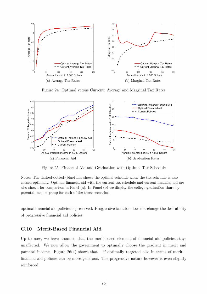
(a) Average Tax Rates (b) Marginal Tax Rates
Figure 24: Optimal versus Current: Average and Marginal Tax Rates
(a) Financial Aid (b) Graduation Rates
Figure 25: Financial Aid and Graduation with Optimal Tax Schedule
Notes: The dashed-dotted (blue) line shows the optimal schedule when the tax schedule is alsochosen optimally. Optimal financial aid with the current tax schedule and current financial aid arealso shown for comparison in Panel (a). In Panel (b) we display the college graduation share byparental income group for each of the three scenarios.
optimal financial aid policies is preserved. Progressive taxation does not change the desirabilityof progressive financial aid policies.
C.10 Merit-Based Financial Aid
Up to now, we have assumed that the merit-based element of financial aid policies staysunaffected. We now allow the government to optimally choose the gradient in merit andparental income. Figure 26(a) shows that – if optimally targeted also in terms of merit –financial aid policies can be more generous. The progressive nature however is even slightlyreinforced.
76

(a) Financial Aid (b) Illustration of Optimal Merit Based Element
Figure 26: Optimal Need and Merit Based Financial Aid
Notes: The dashed-dotted (blue) line shows the optimal financial aid for students with medianability as a function of income when the merit-based component of financial aid is also chosenoptimally. Optimal financial aid with exogenous wage rates and current financial aid are also shownfor comparison in Panel (a). In Panel (b) the merit based component of the optimal aid schedule.
Figure 26(b) shows how optimal financial aid is increasing in AFQT. Interestingly, the slopeis almost independent of parental income.
77