OPTIMAL MASS TRANSPORT ON METRIC GRAPHS - …mate.dm.uba.ar/~jrossi/TransportQuatumGraphs_11_11… · · 2014-11-12OPTIMAL MASS TRANSPORT ON METRIC GRAPHS J. M. MAZON, ... of p

OPTIMAL MASS TRANSPORT ON METRIC GRAPHS

J. M. MAZON, J. D. ROSSI AND J. TOLEDO

Abstract. We study an optimal mass transport problem between two equal

masses on a metric graph where the cost is given by the distance in the

graph. To solve this problem we find a Kantorovich potential as the limitof p−Laplacian type problems in the graph where at the vertices we impose

zero total flux boundary conditions. In addition, the approximation procedure

allows us to find a transport density that encodes how much mass has to betransported through a given point in the graph, and also provide a simple

formula of convex optimization for the total cost.

November 12, 2014

1. Introduction

A quantum graph is a metric graph in which we associate a differential law witheach edge that models the interaction between the two vertices (we denote by vthe vertices in what follows) defining each edge (that we denote by e). The use ofquantum graphs (in contrast to more elementary graph models, such as simple un-weighted or weighted graphs) opens up the possibility of modeling the interactionsbetween agents identified by the graph’s vertices in a far more detailed manner thanwith standard graphs. Quantum graphs are now widely used in physics, chemistryand engineering (nanotechnology) problems, but can also be used, in principle, inthe analysis of complex phenomena taking place on large complex networks, in-cluding social and biological networks. Such graphs are characterized by highlyskewed degree distributions, small diameter and high clustering coefficients, andthey have topological and spectral properties that are quite different from those ofthe highly regular graphs, or lattices arising in physics and chemistry applications.Quantum graphs are also used to model thin tubular structures, so-called graph-likespaces, they are their natural limits, when the radius of a graph-like space tends tozero. On both, the graph-like spaces and the metric graph, we can naturally defineLaplace-like differential operators, [2, 3, 10, 15].

In this paper we are interested in the Monge-Kantorovich mass transport prob-lem on metric graphs. That is, we want to transport a certain amount of material inthe graph to a prescribed final distribution minimizing a cost given by the distanceinside the graph. Our approach to this problem is based on an idea by Evans andGangbo, [7], that approximates a Kantorovich potential for a transport problem inthe Euclidean space with cost given by the Euclidean distance using the limit asp goes to infinity of a family of p−Laplacian type problems. This limit procedureturns out to be quite flexible and allowed us to deal with different transport prob-lems (like optimal matching problems, problems with taxes, etc) in which the cost

Key words and phrases. p−Laplacian, metric graphs, optimal transport, convex optimization.J. M. Mazon and J. Toledo are partially supported by MTM2012-31103 (Spain) and J. D. Rossi

by MTM2011-27998 (Spain).

1

2 J. M. MAZON, J. D. ROSSI AND J. TOLEDO

is given by the Euclidean distance or variants of it. See [8, 11, 12, 13, 14]. Herewe apply these ideas to the optimal transport problem on a metric graph showingagain that this approximation procedure is quite powerful since it provides all therelevant information for the transport problem.

To put our optimal mass transport in modern mathematical terms we have tointroduce some notation. Let Γ be a metric graph (see Section 2 for a precisedefinition) and consider two nonnegative measures on the graph µ and ν with thesame total mass, that is, ∫

Γ

µ =

∫Γ

ν.

The associated optimal transport problem (in its relaxed version, also known asMonge-Kantorovich mass transport problem) reads as follows: find an optimaltransport plan, that is, a measure γ(x, y) that solves the minimization problem

minγ∈Π(µ,ν)

∫Γ

∫Γ

dΓ(x, y) dγ(x, y)

where dΓ(·, ·) is the distance in the metric graph and Π(µ, ν) is the set of measuresthat have marginals µ and ν in the first and second variable respectively. A simpleargument using a minimizing sequence shows that there exists an optimal transportplan γ∗.

This minimization problem has a dual formulation: to find a Kantorovich po-tential u, that is, a function that solves the maximization problem

maxu∈KdΓ

(Γ)

∫Γ

u dη

where

η = µ− ν,and KdΓ(Γ) is the set of 1−Lipschitz functions on Γ, that is, functions u : Γ 7→ Rsuch that |u(x)− u(y)| ≤ dΓ(x, y) for every x, y ∈ Γ.

We can find a Kantorovich potential by an approximation procedure using asequence of solutions up to p−Laplacian type problems and taking the limit asp→∞.

Let us consider solutions to the variational problem

minu∈Sp

1

p

∫Γ

|u′|p −∫

Γ

u dη,

where

Sp :=

u ∈W 1,p(Γ) :

∫Γ

u = 0

.

Such minimizers up are, in fact, weak solutions to (see the notation afterwards):−(|u′|p−2u′)′ = η on edges,∑e∈Ev(Γ)

∣∣∣∣ ∂u∂xe

∣∣∣∣p−2∂u

∂xe(v) = 0 on vertices.

Our first result reads as follows:

Theorem 1.1. There exists a subsequence pj →∞ such that

upj ⇒ u∞

OPTIMAL MASS TRANSPORT ON METRIC GRAPHS 3

uniformly in Γ. The limit u∞ ∈ Kd is a Kantorovich potential for the optimal masstransport problem of µ and ν.

Next, we observe that our approximation procedure gives much more, it allowsus to construct a transport density and to provide simple formulas for the totalcost. These are the contents of our second result. See Section 2 for notation. Letus write η as a measure supported on the edges, denoted by e, plus a sum of deltassupported on the vertices, denoted by v, that is,

(1.1) η = µ+∑

v∈V(Γ)

avδv,

where where av ∈ R and µ is a Radon measure on Γ of the form

〈µ, ϕ〉 =∑

e∈E(Γ)

∫ è

0

[ϕ]edµe for ϕ ∈ C(Γ),

with µe a Radon mesasures in (0, è). Assume the mass balance,∫

Γη = 0, is

satisfied. This gives, ∫Γ

dµ+∑

v∈V(Γ)

av = 0.

Theorem 1.2. Along a subsequence pj →∞ we have that

|[up]′(x)|p−2 → a(x) ∀x ∈ Γ.

This limit function a ∈ L∞(Γ), is a transport density for our problem and verifies|[u∞]′| = 1 in a > 0.

Moreover, we obtain the following simple formula of convex optimization:

Wµ,av = min

∑e∈E(Γ)

∫ è

0

∣∣∣∣ae,ie +

∫ x

0

dµe(y)

∣∣∣∣ dx : ae,v solve (Lµ,av)

for the total cost, Wµ,av , of the optimal transport problem. Here (Lµ,av) stands forthe following system of linear equations for unknowns ae,v,

(Lµ,av)

∑v∈e

ae,v = −∫ è

0

dµe for every edge e,∑e∈Ev(Γ)

ae,v = av at every vertex v.

Remark 1.3. There exists a large amount of literature dealing with optimal trans-port problems in networks, see for instance the two excellent Lecture Notes [4]and [5]. We want to point out that the problems studied in these monographsare different to the one we face here. In fact, in those references the authors tryto find an optimal network that minimize some energy functional associated withthe network. In contrast, here the network is given and our aim is to describethe Kantorovich potential and the transport density of a Monge-Kantorovich masstransport problem on the graph represented by the network.

The paper is organized as follows: in Section 2 we collect some preliminaries;in Section 3 we study the limit as p → ∞ in our p−Laplacian approximation andprove Theorem 1.1 and Theorem 1.2. At the end of Section 3 we collect examplesthat illustrate our results.


2. Preliminaries.

2.1. Quantum Graph. We remind here some basic knowledge about quantumgraphs, see for instance [3] and references therein.

A graph Γ consists of a finite or countable infinite set of vertices V(Γ) = viand a set of edges E(Γ) = ej connecting the vertices. A graph Γ is said a finitegraph if the number of edges and the number of vertices are finite. An edge and avertex on that edge are called incident. We will denote v ∈ e when the edge e andthe vertex v are incident. We define Ev(Γ) as the set of all edges incident to v.

We will assume absence of loops, since if these are present, one can break theminto pieces by introducing new intermediate vertices. We also assume absence ofmultiple edges.

A walk is a sequence of edges e1, e2, e3, . . . in which, for each i (except thelast), the end of ei is the beginning of ei+1. A trail is a walk in which no edge isrepeated. A path is a trail in which no vertex is repeated.

From now on we will deal with a connected, compact and metric graph Γ:• A graph Γ is a metric graph if

(1) each edge e is assigned a positive length è ∈ (0,+∞];(2) for each edge e, a coordinate is assigned to each point of it included their

vertices. For that purpose each edge e is identified with an ordered pair(ie, fe) of vertices, being ie and fe the initial and terminal vertex of e respec-tively, which no has a meaning of sense when travelling along the path butallows to define coordinates by means of an increasing function

ce : e → [0, è]x xe

such that, letting ce(ie) := 0 and ce(fe) := è, is exhaustive; xe is called thecoordinate of the point x ∈ e.

• A graph is said to be connected if a path exists between every pair of vertices,that is, a graph which is connected in the usual topological sense.• A compact metric graph is a finite metric graph whose edges have all finite length.

If a sequence of edges ejnj=1 forms a path, its length is defined as∑nj=1 èj .

The length of a metric graph, denoted `(Γ), is the sum of the length of all its edges.For two vertices v and v, the distance between v and v, dΓ(v, v), is defined as the

minimal length of the paths connecting them. Let us be more precise and considerx, y two points in the graph Γ.

-if x, y ∈ e (they belong to the same edge, note that they can be vertices), wedefine the distance-in-the-path-e between x and y as

diste(x, y) := |ye − xe|;

-if x ∈ ea, y ∈ eb, with ea and eb different edges, let P = ea, e1, . . . , en, eb bea path (n ≥ 0) connecting them. Let us call e0 = ea and en+1 = eb. Following thedefinition given above for a path, set v0 the vertex that is the end of e0 and thebeginning of e1 (note that these vertices need not be the terminal and the initialvertices of the edges that are taken into account), and vn the vertex that is theend of en and the beginning of en+1. We will say that the distance-in-the-path-P


between x and y is equal to

diste0(x, v0) +

∑1≤j≤n

èj + disten+1(vn, y).

We define the distance between x and y, that we will denote by

dΓ(x, y),

as the infimum of all the distances-in-paths between x and y.Remark that the distance between two points x and y belonging to the same

edge e can be strictly smaller than |ye − xe|. This happens when there is a pathconnecting them (using more edges than e) with length smaller than |ye − xe|.

A compact metric graph Γ becomes a compact metric measure space with respectto the distance dΓ.

A function u on a metric graph Γ is a collection of functions [u]e defined on(0, è) for all e ∈ E(Γ), not just at the vertices as in discrete models.

Throughout this work,∫

Γu(x)dx or

∫Γu denotes

∑e∈E(Γ)

∫ è0

[u]e(xe) dxe.

Let 1 ≤ p ≤ +∞. We say that u belongs to Lp(Γ) if [u]e belongs to Lp(0, è) forall e ∈ E(Γ) and

‖u‖pLp(Γ):=

∑e∈E(Γ)

‖[u]e‖pLp(0,è) < +∞.

The Sobolev space W 1,p(Γ) is defined as the space of continuous functions u on Γsuch that [u]e ∈W 1,p(0, è) for all e ∈ E(Γ) and

‖u‖pW 1,p(Γ):=

∑e∈E(Γ)

‖[u]e‖pLp(0,è) + ‖[u]e′‖pLp(0,è) < +∞.

The space W 1,p(Γ) is a Banach space for 1 ≤ p ≤ ∞. It is reflexive for 1 < p <∞and separable for 1 ≤ p <∞. Observe that the continuity condition in the definitionofW 1,p(Γ) means that for each v ∈ V(Γ), the function on all edges e ∈ Ev(Γ) assumethe same value at v.

Let Γ be a compact graph and 1 < p < +∞. The injection W 1,p(Γ) ⊂ C(Γ) iscompact.

A quantum graph is a metric graph Γ equipped with a differential operator actingon the edges accompanied by vertex conditions. In this work, we will consider thep−Laplacian differential operators given by

−∆pu(x) := −(|u′(x)|p−2u′(x))′, with p > 1,

on each edge.

The Monge-Kantorovich problem. Fix µ, ν ∈ M+(Γ) satisfying the massbalance condition

(2.1) µ(Γ) = ν(Γ).

The Monge-Kantorovich problem is the minimization problem

min

∫Γ×Γ

dΓ(x, y) dγ(x, y) : γ ∈ Π(µ, ν)

,

where Π(µ, ν) := Radon measures γ in Γ× Γ : π1#γ = µ, π2#γ = ν. The ele-ments γ ∈ Π(µ, ν) are called transport plans between µ and ν, and a minimizer


γ∗ an optimal transport plan. Since d is lower semicontinuous, there are optimalplans, that is,

∃ γ∗ = arg minγ∈Π(µ,ν)

∫Γ×Γ

dΓ(x, y) dγ(x, y).

The Monge-Kantorovich problem has a dual formulation that can be stated inthis case as follows (see for instance [16, Theorem 1.14]).

Kantorovich-Rubinstein’s Theorem. Let µ, ν ∈ M+(Γ) be two measuressatisfying the mass balance condition (2.1). Then,

min

∫Γ×Γ

dΓ(x, y) dγ(x, y) : γ ∈ Π(µ, ν)

= sup

∫Γ

u d(µ− ν) : u ∈ KdΓ(Γ)

,

where KdΓ(Γ) := u : Γ 7→ R : u(y)− u(x) ≤ dΓ(y, x). Moreover, there exists u ∈

KdΓ(Γ) such that∫

Γ

u d(µ− ν) = sup

∫Γ

v d(µ− ν) : v ∈ KdΓ(Γ)

.

Such maximizers are called Kantorovich potentials.

Example. As an example of metric graph in connection with this mass transportproblem we can consider the road network in a country which can be consider as ametric graph Γ in which V (Γ) corresponds to the set of important cities and E(Γ)to the roads connecting these cities. Then, for x ∈ e ∈ E(Γ), xe ∈ (0, è), thatrepresents the cost of transporting a unit mass from the city ie to x on the road e,could be given by the distance on that road, but we can also take into accountthe possible tolls by changing the parametrization of the edges, expanding themaccording to the size of the toll in that road.

3. The p-Laplacian approximation.

Theorem 3.1. Let µ, ν ∈ M+(Γ) be two measures satisfying the mass balancecondition (2.1). Take η = µ−ν. Consider the functional Fp : W 1,p(Γ)→ R definedby

Fp(u) :=1

p

∫Γ

|u′|p −∫

Γ

u dη.

Then, there exists a minimizer up of the functional Fp in the set

Sp :=

u ∈W 1,p(Γ) :

∫Γ

u = 0

.

Moreover, a minimizer up is a weak solution of the problem

(3.1)

−(|u′|p−2u′)′ = η on edges∑e∈Ev(Γ)

∣∣∣∣ ∂u∂xe

∣∣∣∣p−2∂u

∂xe(v) = 0 on vertices,

in the sense that up ∈W 1,p(Γ) and∫Γ

|u′p|p−2u′pϕ′ =

∫Γ

ϕdη

for every ϕ ∈W 1,p(Γ).


Observe that in the boundary condition in (3.1) the derivatives are taken in thedirection away from the vertex.

Proof. Let un be a minimizing sequence in Sp. Since∫

Ωun = 0, there exists

xn ∈ Γ such that un(xn) = 0. Suppose xn ∈ e ∈ E(Γ). Then, for x ∈ e,

|un(x)| = |[un]e(xe)− [un]((xn)e)| =∣∣∣ ∫ xe

(xn)e

[un]′e

∣∣∣≤ |xe − (xn)e|1/p

′‖[un]′e‖Lp(0,è) ≤ C‖u′n‖Lp(Γ),

being C independent of p. Now, since un is continuous, we can apply the aboveargument in the edges that share a vertex with e. Since Γ is connected and compact,doing this at all edges, we get

(3.2) supx∈Γ|un(x)| ≤ C‖u′n‖Lp(Γ).

Then, as we have ∣∣∣∣∫Γ

u dη

∣∣∣∣ ≤ C‖u‖L∞(Γ) ≤ C‖u‖W 1,p(Γ),

we get that un is bounded in W 1,p(Γ) and hence (using that∫

Γun = 0) we can

extract a subsequence unj → up weakly in W 1,p(Γ) and uniformly in Γ. Then, we

have∫

Γup = 0 and

Fp(up) ≤ lim infjFp(unj ),

and we conclude that up is the desired minimizer.To prove that a minimizer is a weak solution to (3.1) we just observe that when

we differentiate with respect to t at t = 0 the function Fp(up + tϕ) we obtainup ∈W 1,p(Γ) and ∫

Γ


∫Γ

ϕdη, ∀ϕ ∈W 1,p(Γ).

This ends the proof.

Now, we show that there is a limit as p→∞ of the minimizers up.

Lemma 3.2. Let up be a minimizer of the functional Fp on Sp, p > 1. Thereexists a subsequence pj →∞ such that

upj ⇒ u∞

uniformly in Γ. Moreover, the limit u∞ is Lipschitz continuous and ‖u′∞‖L∞(Γ) ≤ 1.

Proof. Along this proof we will denote by C a constant independent of p that maychange from one line to another.

Our first aim is to prove that the Lp-norm of the gradient of up is boundedindependently of p. Since up is a minimizer of Fp on Sp, then,

Fp(up) =

∫Γ

∣∣u′p∣∣p

p

−∫

Γ

up dη ≤ Fp(0) = 0.

That is, ∫Γ

∣∣u′p∣∣p

p

≤∫

Γ

up dη.


Now, from the same arguments leading to (3.2), we obtain∫Γ

up dη ≤ C‖u′p‖Lp(Γ).

Then we get ∫Γ

∣∣u′p∣∣p

p

≤ C‖u′p‖Lp(Γ).

From this inequality, and using that (pC)1/(p−1) → 1 (since C is independent of p)we obtain that

(3.3) ‖u′p‖Lp(Γ) ≤ C,

with C a constant independent of p. Now, by (3.2) and (3.3), we obtain that

(3.4) supx∈Γ|up(x)| ≤ C,

with C a constant independent of p.Using this uniform bound, we prove uniform convergence of a sequence upj . In

fact, we take m such that 1 < m ≤ p and obtain the following bound

‖u′p‖Lm(Γ) =

(∫Γ

∣∣u′p∣∣m · 1) 1m

≤

[(∫Γ

∣∣u′p∣∣p)mp(∫

Γ

1

) p−mp

] 1m

≤ C`(Γ)p−mpm ≤ C,

the constants C being independent of p. We have proved that upp>1 is boundedin W 1,m(Γ), so we can obtain a weakly convergent sequence upj u∞ ∈W 1,m(Γ)

with pj → +∞. Since W 1,p(Γ) is compactly embedded in C(Γ) and upj u∞ ∈W 1,p(Γ), we obtain upj → u∞ uniformly in Γ. Using a diagonal procedure we

conclude the existence of sequence upj that is weakly convergent in W 1,m(Γ) forevery m.

Finally, let us show that the limit function u∞ is Lipschitz. In fact, we have that(∫Γ

|u′∞|m) 1m

≤ lim infpj→+∞

(∫Γ

∣∣∣u′pj ∣∣∣m) 1m

≤ `(Γ)1m .

Now, we take m → ∞ to obtain ‖u′∞‖L∞(Γ) ≤ 1. So, we have proved that u∞ ∈W 1,∞(Γ), that is, u∞ is a Lipschitz function and ‖u′∞‖L∞(Γ) ≤ 1.

Theorem 3.3. Any uniform limit u∞ of a sequence upj is a Kantorovich potentialfor the optimal transport problem of µ to ν with the cost given dΓ, that is, it holdsthat

min

∫Γ×Γ

dΓ(x, y) dγ(x, y) : γ ∈ Π(µ, ν)

= sup

∫Γ

u d(ν − µ) : u ∈ KdΓ(Γ)

=

∫Γ

u∞ d(µ− ν).


Proof. By the Kantorovich-Rubinstein’s Theorem, we only need to show the lastequality. To do that, first let us see that

(3.5) KdΓ(Γ) =

u ∈W 1,∞(Γ) : ‖u′‖L∞(Γ) ≤ 1

.

It is easy to see that

KdΓ(Γ) ⊂ LipdΓ

(Γ) =u ∈W 1,∞(Γ) : ‖u′‖L∞(Γ) ≤ 1

.

Let us see the reverse inclusion. Let

u ∈u ∈W 1,∞(Γ) : ‖u′‖L∞(Γ) ≤ 1

and x, y ∈ Γ with x ∈ ea and y ∈ eb. Suppose that dΓ(x, y) is attained at the pathe0, e1, . . . , en, en+1, n ≥ −1, where ea = e0 and eb = en+1. Suppose fe0

is thevertex that is the end of e0 and the beginning of e1, and ien+1 the vertex that is theend of en and the beginning of en+1, for other cases the argument is similar. Then,we have

dΓ(x, y) = |ye0 − xe0 | if n = −1,

dΓ(x, y) = le0 − xe0 +∑

1≤i≤n

èi + yen+1 if n ≥ −1.

Now, if n = −1

|u(x)− u(y)| = |[u]e0(xe0)− [u]e0(ye0)| ≤ |ye0 − xe0 | = dΓ(x, y),

and if n ≥ 0,

|u(x)− u(fe0)| = |[u]e0

(xe0)− [u]e0

(è0)| ≤ è0

− xe0,

|u(iei)− u(fei)| = |[u]ei(0)− [u]ei(èi)| ≤ èi+1 , 1 ≤ i ≤ n,and

|u(ien+1)− u(y)| = |[u]en+1(0)− [u]en+1(yen+1)| ≤ yen+1 .

Hence,

|u(x)− u(y)| ≤ |u(x)− u(fe0)|+

∑1≤i≤n

|u(iei)− u(fei)|+ |u(ien+1)− u(y)|

≤ è0 − xe0 +∑

1≤i≤n

èi + yen+1 = dΓ(x, y).

Consequently, (3.5) holds.Due to (3.5), we just need to show that

(3.6) sup

∫Γ

v d(µ− ν) : v ∈ LipdΓ

=

∫Γ

u∞ d(µ− ν).

Given v ∈ LipdΓ(Γ), if we define

v := v − 1

`(Γ)

∫v dx.

We have v ∈ Sp, then

Fp(up) =

∫Γ

∣∣u′p∣∣p

p

−∫

Γ

up dη ≤ Fp(v)

=

∫Γ

|v′|p

p

−∫

Γ

v dη ≤ 1

p`(Γ)−

∫Ω

v dη.


Therefore,

−∫

Γ

up dη ≤∫

Γ

∣∣u′p∣∣p

p

−∫

Γ

up dη ≤∫

Γ

|v′|p

p

−∫

Γ

v dη ≤ 1

p`(Γ)−

∫Γ

v dη.

Taking limits as p→∞ we obtain∫Γ

u∞ d(µ− ν) ≥∫

Γ

v d(µ− ν)

and consequently, we get∫Γ

u∞ d(µ− ν) ≥ sup

∫Γ

v d(µ− ν) : v ∈ LipdΓ(Γ)

,

from where it follows (3.6), since u∞ ∈ Lipd(Γ).

In order to find the transport density we need the following result.

Lemma 3.4. Let µ = µ+−µ−, µ± positive Radon measure in (a, b), and α, β ∈ Rsatisfying ∫ b

a

dµ+ α+ β = 0.

(i) For any p > 1 let vp be a weak solution of the problem

(3.7)

−(|v′|p−2v′

)′= µ in (a, b),(

|v′|p−2v′)

(a) = −α,(|v′|p−2v′

)(b) = β.

If

vp ⇒ v∞

uniformly in [a, b] with ‖v′∞‖L∞(a,b) ≤ 1, then v∞ is a Kantorovich potential

for the optimal transport problem of η+ := µ+ + (α+δa + β+δb) to η− :=µ− + (α−δa + β−δb) with the cost given by the Euclidean distance.

(ii) If there exists a nonnegative function a ∈ L∞(a, b) and a Lipschitz con-tinuous function u, with ‖u′‖L∞(a,b) ≤ 1, such that u is a weak solution

of

(3.8)

−(au′)′ = µ in (a, b),

au′(a) = −α,

au′(b) = β,

in the sense ∫ b

a

au′ϕ′ −∫ b

a

ϕdµ = αϕ(a) + βϕ(a)

for all ϕ ∈W 1,∞(0, è), and verifies

|u′| = 1 on a > 0,

then u is a Kantorovich potential for the optimal transport problem of η+

to η− with the cost given by the Euclidean distance.


Proof. (i) Since vp be a weak solution of the problem (3.7), we have

(3.9)

∫ b

a

(|v′p|p−2v′p

)w′ =

∫ b

a

w dµ+ αw(a) + βw(b), ∀w ∈W 1,p(]a, b[).

Taking w = vp in (3.9), we obtain∫ b

a

|v′p|p =

∫ b

a

vp dµ+ αvp(a) + βvp(b) ≤ C.

Given v ∈W 1,∞(]a, b[) with ‖v′‖∞ ≤ 1, taking w = vp − v in (3.9), we get∫ b

a

|v′p|p −∫ b

a

(|v′p|p−2v′p

)v′

=

∫ b

a

(vp − v)dµ+ α(vp(a)− v(a)) + β(vp(b)− v(b)).

Hence ∫ b

a

vpη −∫ b

a

vη =

∫ b

a

|v′p|p −∫ b

a

(|v′p|p−2v′p

)v′.

Now, by Young’s inequality, we have∫ b

a

(|v′p|p−2v′p

)v′ ≤ p− 1

p

∫ b

a

|v′p|p +1

p

∫ b

a

|v′|p

≤ p− 1

p

∫ b

a

|v′p|p +1

p(b− a).

Therefore, we obtain∫ b

a

vp dη −∫ b

a

v dη ≥ 1

p

∫ b

a

|v′p|p −1

p(b− a) ≥ −1

p(b− a).

Taking limits as p→∞ we get∫ b

a

v∞ dη ≥∫ b

a

v dη

and consequently∫ b

a

v∞ dη = sup

∫ b

a

vdη : v ∈W 1,∞(]a, b[) with ‖v′‖∞ ≤ 1

.

This ends the proof of (i).

(ii) Taking u as test function in (3.8), we get that∫ b

a

udµ+ αu(0) + βu(b) =

∫ b

a

a.

Take now a Lipschitz continuous function u , with ‖u′‖L∞(a,b) ≤ 1, as test function

in (3.8). Then ∫ b

a

udµ+ αu(a) + βu(b) =

∫ b

a

au′u′

≤∫ b

a

a =

∫ b

a

udµ+ αu(0) + βu(b),

which gives the assertion.


Suppose now that η is as in (1.1) and take up as in Theorem 3.1. Then, up ∈W 1,p(Γ) and ∫

Γ


∑e∈Ev(Γ)

∫ è

0

[ϕ]edµe +∑

v∈V(Γ)

avϕ(v)

for every ϕ ∈ W 1,p(Γ). For a fixed edge e ∈ E(Γ), we define the distribution ηp,ein R as

〈ηp,e, ϕ〉 :=

∫ è

0

|[up]′e|p−2[up]′eϕ′ −∫ è

0

ϕdµe, for all ϕ ∈ C∞c (R).

Theorem 3.5. For up as above, measures ηp,e, and u∞ as in Lemma 3.2, we have:

(1) For each edge e ∈ E(Γ) the following facts hold:(a) ηp,e is a Radon measure on R supported on 0, è, and consequently

ηp,e = ap,e,ieδ0 + ap,e,feδè , ap,e,ie , ap,e,fe ∈ R;

(b) [up]e is a weak solution of

(3.10)

−(|u′|p−2u′

)′= µe in (0, è),∣∣∣∣ ∂u∂xe

∣∣∣∣p−2∂u

∂xe(0) = −ap,e,ie ,∣∣∣∣ ∂u∂xe

∣∣∣∣p−2∂u

∂xe(è) = ap,e,fe ;

(c) for a subsequence pi → +∞,

(api,e,ie , api,e,fe)→ (a∞,e,ie , a∞,e,fe);

(d) [u∞]e is a Kantorovich potential for the optimal transport problem ofµ+

e + (a∞,e,ie)+δ0 + (a∞,e,fe)+δè to µ−e + (a∞,e,ie)−δ0 + (a∞,e,fe)−δèwith the cost given by the Euclidean distance.

(2)∑

e∈Ev(Γ)

a∞,e,v = av for any v ∈ V(Γ).

Proof. (1a) Given ϕ ∈ C∞c (R) supported on R \ 0, è, we have∫ è

0

|[up]′e|p−2[up]′eϕ′ −∫ è

0

ϕdµe = 0.

Therefore, ηp,e defines a Radon measure on R supported on 0, è, and conse-quently there exist ap,ie , ap,fe ∈ R such that

ηp,e = ap,e,ieδ0 + ap,e,feδè .

(1b) Given ϕ ∈W 1,p(0, è), let ϕn ∈ C∞c (R) such that

ϕn|(0,è) → ϕ

in W 1,p(0, è). Then∫ è

0

|[up]′e|p−2[up]′eϕ′n −

∫ è

0

ϕndµe = ap,e,feϕn(è) + ap,e,ieϕn(0).


Hence, taking limits as n→∞, we obtain that

(3.11)

∫ è

0

|[up]′e|p−2[up]′eϕ′ −∫ è

0

ϕdµe = ap,e,feϕ(è) + ap,e,ieϕ(0).

Therefore, [up]e is a weak solution of (3.10).

(1c) Let us see that ap,e,iep>1 and ap,e,fep>1 are bounded. Taking in (3.11)ϕ = [up]e, since by (3.4), [up]e is uniformly bounded independent of p, we have

(3.12)

∫ è

0

|[up]′e|p ≤∫ è

0

[up]edµe + ap,e,fe [up]e(è) + ap,e,ie [up]e(0) ≤ C,

for every p > 1.On the other hand, taking ϕ(x) = x in (3.11), we get

ap,e,feè =

∫ è

0

|[up]′e|p−2[up]′e −

∫ è

0

x dµe(x).

Then, by (3.12) and using Holder’s inequality, we get that ap,e,fep>1 is bounded.Finally, taking ϕ = 1 in (3.11) we get ap,e,ie is bounded.

(1d) From the compatibility condition of problem (3.10), we have∫ è

0

dµe + ap,e,ie + ap,e,fe = 0.

Taking limit as p→∞ we obtain∫ è

0

dµe + a∞,e,ie + a∞,e,fe = 0.

Then, by Lemma 3.4, we have that [u∞]e is a Kantorovich potential for the optimaltransport problem of [µ+]e + (a∞,e,ie)+δ0 + (a∞,e,fe)+δè to [µ−]e + (a∞,e,ie)−δ0 +(a∞,e,fe)−δè with the cost given by the Euclidean distance.

(2) Given ϕ ∈W 1,p(Γ), since up is a weak solution of (3.1), adding (3.11) for alle ∈ E(Γ), ∑

e∈E(Γ)

(ap,e,fe [ϕ]e(è) + ap,e,ie [ϕ]e(0)) =∑

v∈V(Γ)

avϕ(v).

Letting p→ +∞ we get∑e∈E(Γ)

(a∞,e,fe [ϕ]e(è) + a∞,e,ie [ϕ]e(0)) =∑

v∈V(Γ)

avϕ(v).

Then, rearranging the terms,∑v∈V(Γ)

∑e∈Ev(Γ)

a∞,e,vϕ(v) =∑

v∈V(Γ)

avϕ(v),

from where we get the desired conclusion.

Observe that a∞,e,v are solutions of the following system of linear equations forunknowns ae,v:

(Lµ,av)

∑v∈e

ae,v = −∫ è

0

dµe ∀e ∈ E(Γ),∑e∈Ev(Γ)

ae,v = av ∀v ∈ V(Γ).


For any solution ae,v of (Lµ,av), we define

Cµ,av(ae,v) :=∑

e∈E(Γ)

W1

((µe +

∑v∈e

[ae,vδv]e

)+

,(µe +

∑v∈e

[ae,vδv]e

)−),

where ∑v∈e

[ae,vδv]e = ae,ieδ0 + ae,feδè ,

and W1 is the Wasserstein distance in R respect to the cost c(x, y) = |x − y|. Inthe next result we shall see how to solve the transport problem in graphs throughthe a∞,e,v and the functional Cµ,av

.

Theorem 3.6. Let η be a measure given by (1.1). Under the assumptions of The-orem 3.5 and for a∞,e,ve ∈ E(Γ)

v ∈ e

given there, we have that

(3.13) a∞,e,ve ∈ E(Γ)v ∈ e

∈ arg minae,v solve (Lµ,av )

Cµ,av(ae,v).

Moreover

(3.14)

Wµ,av = min

∫Γ×Γ

dΓ(x, y)dσ(x, y) : σ ∈ Π(η+, η−

)=

∫Γ

u∞

(µ+

∑v∈V(Γ)

avδv

)= minae,v solve (Lµ,av )

Cµ,av(ae,v)

= Cµ,av(a∞,e,v).

Proof. Since a∞,e,v are solutions of (Lµ,av), we have∫

Γ

u∞

( ∑v∈V(Γ)

avδv

)=

∑v∈V(Γ)

avu∞(v) =∑

v∈V(Γ)

( ∑e∈Ev(Γ)

a∞,e,v

)u∞(v),

and, rearranging, ∫Γ

u∞

( ∑v∈V(Γ)

avδv

)=

∑e∈E(Γ)

∑v∈e

a∞,e,vu∞(v).

Therefore,∫Γ

u∞

(µ+

∑v∈V(Γ)

avδv

)=

∑e∈E(Γ)

(∫ è

0

[u∞]edµe + a∞,e,ie [u∞]e(0) + a∞,e,fe [u∞]e(è)).

Now, since [u∞]e is a Kantorovich potential for the optimal transport problem of[µ+]e + (a∞,e,ie)+δ0 + (a∞,e,fe)+δè to [µ−]e + (a∞,e,ie)−δ0 + (a∞,e,fe)−δè with the


cost given by the Euclidean distance, we have∫ è

0

[u∞]edµe + a∞,e,ie [u∞]e(0) + a∞,e,fe [u∞]e(è)

= W1

(µe +∑v∈e

[a∞,e,vδv]e

)+

,

(µe +

∑v∈e

[a∞,e,vδv]e

)− .

Consequently,∫Γ

u∞

(µ+

∑v∈V(Γ)

avδv

)=

∑e∈E(Γ)

W1

((µe +

∑v∈e

[a∞,e,vδv]e

)+

,(µe +

∑v∈e

[a∞,e,vδv]e

)−)= Cµ,av

(a∞,e,v).Hence, for

ae,ve ∈ E(Γ)v ∈ e

∈ arg minae,v solve (Lµ,av )

Cµ,av(ae,v)

we have that∫Γ

u∞

(µ+

∑v∈V(Γ)

avδv

)≥

∑e∈E(Γ)

W1

((µe +

∑v∈e

[ae,vδv]e

)+

,(µe +

∑v∈e

[ae,vδv]e

)−)= Cµ,av

(ae,v).

Given e ∈ E(Γ), let γe be an optimal transport plan between(µ e +

∑v∈e ae,vδv

)+and

(µ e +

∑v∈e ae,vδv

)−with respect to the cost given by the metric dΓ. Then

we have

W1

((µe +

∑v∈e

[ae,vδv]e

)+

,(µe +

∑v∈e

[ae,vδv]e

)−)≥∫

Γ×Γ

dΓ(x, y)dγe(x, y).

Hence, if γ :=∑

e∈E(Γ) γe, we get

Cµ,av(ae,v) =∑

e∈E(Γ)

W1

((µe +

∑v∈e

[ae,vδv]e

)+

,(µe +

∑v∈e

[ae,vδv]e

)−)≥∫

Γ×Γ

dΓ(x, y)dγ(x, y).

Now, given ϕ ∈ C(Γ), we have∫Γ

ϕ(x)dπ1#γ(x) =

∫Γ×Γ

ϕ(x)dγ(x, y) =∑

e∈E(Γ)

∫Γ×Γ

ϕ(x)dγe(x, y)

=∑

e∈E(Γ)

∫Γ

ϕ(x)d(µ e +

∑v∈e

ae,vδv

)+

=∑

e∈E(Γ)

(∫ è

0

[ϕ]e(x)dµe +∑v∈e

a+e,vϕ(v)

).


Since ∑e∈E(Γ)

∑v∈e

a+e,vϕ(v) =

∑v∈V (Γ)

a+v ϕ(v) =

∫Γ

ϕ(x)d( ∑

v∈V(Γ)

avδv

)+

,

we get

π1#γ =(µ+

∑v∈V(Γ)

avδv

)+

.

Similarly, we obtain

π2#γ =(µ+

∑v∈V(Γ)

avδv

)−.

Consequently,

γ ∈∏(µ+

∑v∈V(Γ)

avδv

)+

,(µ+

∑v∈V(Γ)

avδv

)− .

Therefore, ∫Γ

u∞

(µ+

∑v∈V(Γ)

avδv

)= min

∫Γ×Γ

dΓ(x, y)dσ(x, y) : σ ∈ Π(η+, η−

)≤∫

Γ×Γ

dΓ(x, y)dγ(x, y) ≤ Cµ,av(ae,v)

≤ Cµ,av(a∞,e,v)

=

∫Γ

u∞

(µ+

∑v∈V(Γ)

avδv

)from where we get (3.13) and (3.14).

Remark 3.7. Observe that (3.14) imply that each a∞,e,v is the mass that en-ters/leaves e via the vertex v ∈ e, depending on its positive/negative sign, duringthe optimal transport process.

Remark 3.8. In the particular case of µ ≡ 0 we get the even simpler formula

a∞,e,ve ∈ E(Γ)v ∈ e

∈ arg min

1

2

∑e∈E(Γ)

(∑v∈e

|ae,v|

)è : ae,v solve (L0,av)

,

and

W0,av = min

1

2

∑e∈E(Γ)

(∑v∈e

|ae,v|

)è : ae,v solve (L0,av)

for the optimal total cost of the transport problem. Observe that we can rewritethis as follows:

W0,av = min

∑e∈E(Γ)

|ae,ie |è : ae,v solve (L0,av)

.


Moreover, since

ap,e,ie + ap,e,fe = 0,

we have [up]e is a weak solution of

−(|u′|p−2u′

)′= 0 in (0, è),∣∣∣∣ ∂u∂xe

∣∣∣∣p−2∂u

∂xe(0) = −ap,e,ie ,∣∣∣∣ ∂u∂xe

∣∣∣∣p−2∂u

∂xe(è) = −ap,e,ie .

Therefore, up to a constant,

[up]e(x) = −sign(ap,e,ie)|ap,e,ie |1p−1x,

and consequently, up to a constant,

[u∞]e(x) = −sign(a∞,e,ie)x.

A remarkable fact is that our results show that these functions can be glued con-tinuously on the graph Γ.

In the next result we shall see that also in the case µ 6= 0 it is possible to get asimple formula for the total cost. We also find a transport density for the transportproblem.

Theorem 3.9. Let η be a measure given by (1.1). Under the assumptions of The-orem 3.5 and for a∞,e,ve ∈ E(Γ)

v ∈ e

given there, there exists a nonnegative function

a ∈ L∞(Γ) such that [u∞]e is a weak solution of

(3.15)

−([a]e[u∞]′e)′ = µe in (0, è),

[a]e[u∞]′e(0) = −a∞,e,ie ,

[a]e[u∞]′e(è) = a∞,e,fe ,

in the sense ∫ è

0

[a]e[u∞]′eϕ′ −∫ è

0

ϕdµe = a∞,e,feϕ(è) + a∞,e,ieϕ(0)

for all ϕ ∈W 1,∞(0, è). Furthermore,

(3.16) |[u∞]′e| = 1 on [a]e > 0.

More precisely, we have

(3.17) [a]e(x) =

∣∣∣∣a∞,e,ie +

∫ x

0

dµe(y)

∣∣∣∣ for x ∈ (0, è)

and

(3.18) [u∞]′e(x) = sign

(−a∞,e,ie −

∫ x

0

dµe(y)

)for x ∈ (0, è).


Moreover, it holds that the optimal total cost is given by

(3.19)

Wµ,av= min

∑e∈E(Γ)

∫ è

0

∣∣∣∣ae,ie +

∫ x

0

dµe(y)

∣∣∣∣ dx : ae,v solve (Lµ,av)

=

∑e∈E(Γ)

∫ è

0

∣∣∣∣a∞,e,ie +

∫ x

0

dµe(y)

∣∣∣∣ dx.Proof. Fix e ∈ E(Γ), and take [up]e the weak solution obtained above. Then, from(3.10) we have

−(|[up]′e|p−2[up]

′e

)′= µe in D′(0, è).

Now, we let

wµ,e(x) := µe((0, x)) =

∫ x

0

dµe(y)

for x ∈ (0, è) and we observe that (wµ,e)′ = µe in D′(0, è). Hence, there exists aconstant αp,e ∈ R such that |[up]′e|p−2[up]

′e = −wµ,e + αp,e. Then, since

−ap,e,ie = |[up]′e|p−2[up]′e(0) = −wµ,e(0) + αp,e = αp,e,

we get|[up]′e|p−2[up]

′e(x) = −wµ,e(x)− ap,e,ie .

Now we observe that −wµ,e(x) − ap,e,ie is bounded in L∞ uniformly in p, andthat, for a subsequence,

|[up]′e(x)|p−2 = |wµ,e(x) + ap,e,ie |p−2p−1 → |wµ,e(x) + a∞,e,ie | =: [a]e(x) ∀x ∈ (0, è).

Moreover, by (3.12), we can assume that

[up]′e [u∞]′e weakly in L2((0, è)).

Therefore, we have that

|[up]′e|p−2[up]′e → |wµ,e + a∞,e,ie | [u∞]′e in L1((0, è)),

but also|[up]′e|p−2[up]

′e → −wµ,e − a∞,e,ie .

Consequently, (3.16), (3.17) and (3.18) are proved.On the other hand, by (3.11), for any ϕ ∈W 1,∞(0, è), we have

(3.20)

∫ è

0

|[up]′e|p−2[up]′eϕ′ −∫ è

0

ϕdµe = ap,e,feϕ(è) + ap,e,ieϕ(0).

Then, taking limits in (3.20) when p→∞, we get∫ è

0

[a]e[u∞]′eϕ′ −∫ è

0

ϕdµe = a∞,e,feϕ(è) + a∞,e,ieϕ(0)

for all ϕ ∈W 1,∞(0, è), and thus (3.15) holds.Let ae,v a solution of (Lµ,av

). Then, if we define

a(x) =

∣∣∣∣ae,ie +

∫ x

0

dµe(y)

∣∣∣∣ for x ∈ (0, è),

and u by

u′(x) = sign

(−ae,ie −

∫ x

0

dµe(y)

)for x ∈ (0, è),


we have, 0 ≤ a ∈ L∞(0, è) and u is a Lipschitz function with ‖u′‖L∞(0,è) ≤ 1,

such that u is a weak solution of

(3.21)

−(au′)′ = µe in (0, è),

au′(0) = −ae,ie ,

au′(è) = ae,fe ,

and

|u′| = 1 on a > 0.Then by (ii) in Lemma 3.4, u is a Kantorovich potential for the transport of(µe +

∑v∈e[ae,vδv]e

)+to(µe +

∑v∈e[ae,vδv]e

)−. Therefore, taking u as test func-

tion in (3.21), we get∫ è

0

a|u′|2 −∫ è

0

udµe = ae,fe u(è) + ae,ie u(0),

and consequently∫ è

0

∣∣∣∣ae,ie +

∫ x

0

dµe(y)

∣∣∣∣ dx = −∫ è

0

udµe + ae,fe u(è) + ae,ie u(0)

= W1

((µe +

∑v∈e

[ae,vδv]e

)+

,(µe +

∑v∈e

[ae,vδv]e

)−).

Adding, we obtain∑e∈E(Γ)

∫ è

0

∣∣∣∣ae,ie +

∫ x

0

dµe(y)

∣∣∣∣ dx = Cµ,av(ae,v),

from where (3.19) follows having in mind (3.14).

Remark 3.10. The first part of the above result is similar to Lemma 7.2 in [1] themain difference is that here we have to consider fluxes at the ends of the edges.

Finally, let us present some simple examples to illustrate our results.

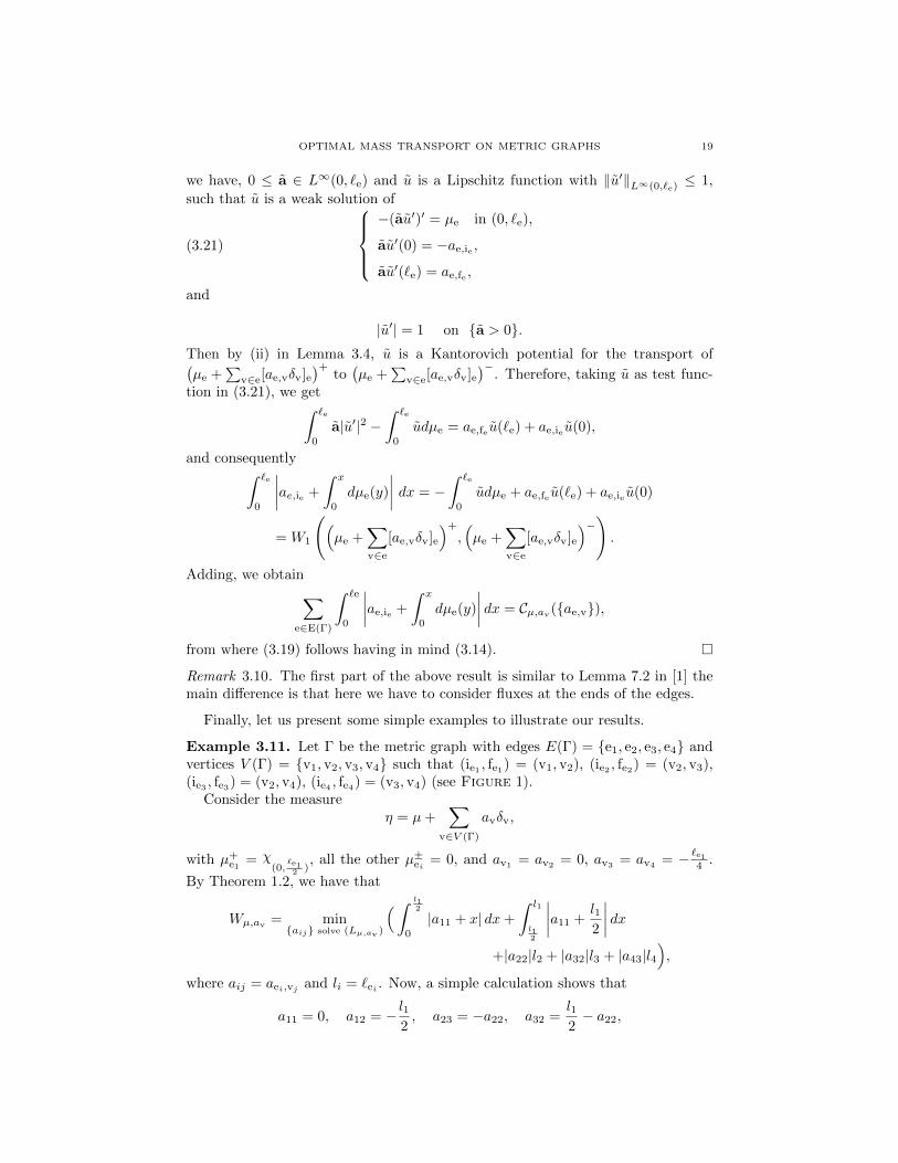
Example 3.11. Let Γ be the metric graph with edges E(Γ) = e1, e2, e3, e4 andvertices V (Γ) = v1, v2, v3, v4 such that (ie1

, fe1) = (v1, v2), (ie2

, fe2) = (v2, v3),

(ie3, fe3

) = (v2, v4), (ie4, fe4

) = (v3, v4) (see Figure 1).Consider the measure

η = µ+∑

v∈V (Γ)

avδv,

with µ+e1

= χ(0,

è12 )

, all the other µ±ei = 0, and av1= av2

= 0, av3= av4

= − è1

4 .

By Theorem 1.2, we have that

Wµ,av= minaij solve (Lµ,av )

(∫ l12

0

|a11 + x| dx+

∫ l1

l12

∣∣∣∣a11 +l12

∣∣∣∣ dx+|a22|l2 + |a32|l3 + |a43|l4

),

where aij = aei,vj and li = èi . Now, a simple calculation shows that

a11 = 0, a12 = − l12, a23 = −a22, a32 =

l12− a22,


and

a34 = a22 −l12, a43 = a22 −

l14, a44 =

l14− a22.

Hence, the total cost is given by

Wµ,av= mina22∈R

(3

8l21 + |a22|l2 +

∣∣∣∣a22 −l12

∣∣∣∣ l3 +

∣∣∣∣a22 −l14

∣∣∣∣ l4) .We have different values for the minimum depending on the values of l2, l3, l4:

(1) If l2 > l3 + l4 then the minimum is attained at a22 = 0. Consequently, asexpected, the route of the optimal transport is given in Figure 1. Note that weare not sending mass trough e2, but instead we use e3 until we reach v4 where wedeposit half of the mass and then continue trough e4 until reaching v3 with theother half of the mass.

v1

v2

v4

v3

e1

e2

e3

e4

Figure 1. Optimal transport path for l2 > l3 + l4

In this case, the optimal transport cost is given by

Wµ,av=

3

8l1

2 +1

2l1l2 +

1

4l1l4 =

1

2l1

3

4l1 +

1

4l1l3 +

1

4l1(l3 + l4).

(2) If l3 > l2 + l4 then the minimum is attained at a22 = l12 . Hence a32 = 0 and

consequently, in this case, the best strategy is not to use e3 to transport mass.

(3) In other case, the minimum is attained at a22 = l14 . Hence a43 = a44 = 0,

therefore, here we split the mass in two equal parts when we arrive to v2 and sendthem to v3 and v4 using e2 and e3. Now, we are not using e4.

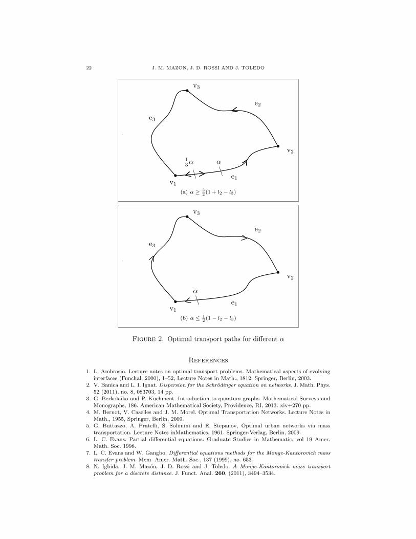
Example 3.12. Let Γ be the metric graph with edges E(Γ) = e1, e2, e3 andvertices V (Γ) = v1, v2, v3 such that (ie1 , fe1) = (v1, v2), (ie2 , fe2) = (v2, v3),(ie3 , fe3) = (v3, v1) (see Figure 2). Take è1 = 1.

Consider the measureη = µ+

∑v∈V (Γ)

avδv,


with µ+e1

= χ(0,α), 0 < α ≤ 1, all the other µ±ei = 0, and av1

= av2= av3

= −α3 . ByTheorem 1.2, we have that

Wµ,av= minaij solve (Lµ,av )

(∫ α

0

|a11 + x| dx

+ |a11 + α| (1− α) + |a22|l2 + |a31|l3),

where aij = aei,vj and li = èi . Now, a simple calculation shows that

a12 = −a11−α, a22 = a11 +2

3α, a23 = −a22, a31 = −a11−

1

3α, a33 = −a31.

Therefore,

Wµ,av= mina11∈R

(∫ α

0

|a11 + x| dx+∣∣∣a11 + α

∣∣∣(1− α)

+∣∣∣a11 +

2

3α∣∣∣l2 +

∣∣∣a11 +1

3α∣∣∣l3).

We have different values for the minimum depending on the values of l2, l3 and α.In fact, preforming a tedious computation we get the following:

(1) If α ≥ 32 (1 + l2 − l3) then the minimum is attained at a11 = − 1

3α. This impliesthat

a12 = −2

3α, a22 =

1

3α, a23 = −1

3α, a31 = a33 = 0.

The path of the optimal transport is given in Figure 2 (a).Note that we are not sending mass trough e3, but instead we use e1 until we reach

v2 where we deposit 13α of the mass and then continue trough e2 until reaching v3

with the other 13α of the mass.

(2) If 34 (1 + l2 − l3) < α < 3

2 (1 + l2 − l3) then the minimum is attained at a11 =12 (l3 − l2 − 1) ∈

(− 2

3α,−13α). Therefore, all the aij 6= 0 and consequently in this

case it is necessary to use all the edges.

(3) If 34 (1− l2− l3) ≤ α ≤ 3

4 (1+ l2− l3) then the minimum is attained at a11 = − 23α.

Hence,

a12 = −1

3α, a22 = a23 = 0, a31 = −1

3α a33 =

1

3α.

Consequently, in this case, the best strategy is not to use e2 to transport mass.

(4) If 12 (1 − l2 − l3) < α < 3

4 (1 − l2 − l3) then the minimum is attained at a11 =12 (l3 + l2 − 1) ∈

(−α,− 2

3α). In this case, the best strategy is not to use e3 to

transport mass.

(5) If α ≤ 12 (1− l2 − l3) then the minimum is attained at a11 = −α. Then, we get

a12 = 0, a22 = −1

3α, a23 =

1

3α, a31 =

2

3α, a33 = −2

3.

In this case we are sending all the mass trough v1 and then use e3 and e2 to deliverit to its final destination at v3 and v2 (see Figure 2 (b)).


v1

v3

v2

e1

e3

e2

13α α

(a) α ≥ 32

(1 + l2 − l3)

v1

v3

v2

e1

e3

e2

α

(b) α ≤ 12

(1 − l2 − l3)

Figure 2. Optimal transport paths for different α

References

1. L. Ambrosio. Lecture notes on optimal transport problems. Mathematical aspects of evolving

interfaces (Funchal, 2000), 1–52, Lecture Notes in Math., 1812, Springer, Berlin, 2003.

2. V. Banica and L. I. Ignat. Dispersion for the Schrodinger equation on networks. J. Math. Phys.52 (2011), no. 8, 083703, 14 pp.

3. G. Berkolaiko and P. Kuchment. Introduction to quantum graphs. Mathematical Surveys and

Monographs, 186. American Mathematical Society, Providence, RI, 2013. xiv+270 pp.4. M. Bernot, V. Caselles and J. M. Morel. Optimal Transportation Networks. Lecture Notes in

Math., 1955, Springer, Berlin, 2009.

5. G. Buttazzo, A. Pratelli, S. Solimini and E. Stepanov, Optimal urban networks via masstransportation. Lecture Notes inMathematics, 1961. Springer-Verlag, Berlin, 2009.

6. L. C. Evans. Partial differential equations. Graduate Studies in Mathematic, vol 19 Amer.Math. Soc. 1998.

7. L. C. Evans and W. Gangbo, Differential equations methods for the Monge-Kantorovich mass

transfer problem. Mem. Amer. Math. Soc., 137 (1999), no. 653.8. N. Igbida, J. M. Mazon, J. D. Rossi and J. Toledo. A Monge-Kantorovich mass transport

problem for a discrete distance. J. Funct. Anal. 260, (2011), 3494–3534.


9. V. Kostrykin, R. Schrader, Kirchhoff’s Rule for Quantum Wires. J. Phys. A 32 (1999), no. 4,

595–630.

10. P. Kuchment, Quantum graphs: I. Some basic structures, Waves Random Media 14 (2004),S107–S128.

11. J. M. Mazon, J. D. Rossi and J. Toledo. An optimal transportation problem with a cost

given by the Euclidean distance plus import/export taxes on the boundary. Revista MatematicaIberoamericana. 30 (2014), 277–308.

12. J. M. Mazon, J. D. Rossi and J. Toledo. An optimal matching problem for the Euclidean

distance. SIAM J. Math. Anal. 46, (2014), 233–255.13. J. M. Mazon, J. D. Rossi and J. Toledo. Mass transport problems for the Euclidean distance

obtained as limits of p−Laplacian type problems with obstacles. J. Diff. Equations, 256 (2014),

3208–3244.14. J. M. Mazon, J. D. Rossi and J. Toledo. Mass transport problems obtained as limits of

p−Laplacian type problems with spatial dependence. Adv. Non. Anal. 3(3), (2014), 133–140.15. O. Post, Spectral Analysis on Graph-Like Spaces. Lecture Notes in Mathematics. 2012.

16. C. Villani. Topics in Optimal Transportation. Graduate Studies in Mathematics. Vol. 58, 2003.

17. C. Villani. Optimal transport. Old and new. Grundlehren der MathematischenWissenschaften(Fundamental Principles of Mathematical Sciences), vol. 338. Springer, Berlin (2009).

J. M. Mazon: Departament d’Analisi Matematica, Universitat de Valencia, Valencia,

Spain. [email protected]

J. D. Rossi: CONICET and Depto de Matematica, FCEyN, Universidad de Buenos

Aires, Pab. I, Ciudad Universitaria (1428), Buenos Aires, Argentina. [email protected]

J. Toledo: Departament d’Analisi Matematica, Universitat de Valencia, Valencia,

Spain. [email protected]

Documents

OPTIMAL MASS TRANSPORT ON METRIC GRAPHS - …mate.dm.uba.ar/~jrossi/TransportQuatumGraphs_11_11… · · 2014-11-12OPTIMAL MASS TRANSPORT ON METRIC GRAPHS J. M. MAZON, ... of p