Optimal learning and experimentation in bandit …steele/Courses/900/Library/Bandits/...Journal of Economic Dynamics & Control 27 (2002) 87–108 Optimal learning and experimentation

Journal of Economic Dynamics & Control27 (2002) 87–108

www.elsevier.com/locate/econbase

Optimal learning and experimentation inbandit problems

Monica Brezzia, Tze Leung Laib;∗;1aDipartimento per le politiche di sviluppo e coesione, Ministero del Tesoro Via Nerva

1-00187 Rome, ItalybDepartment of Statistics, Sequoia Hall, Stanford University, Stanford,

CA 94305-4065, USA

Received 10 January 2000; accepted 2 April 2001

Abstract

This paper studies how and how much active experimentation is used in discountedor 0nite-horizon optimization problems with an agent who chooses actions sequen-tially from a 0nite set of actions, with rewards depending on unknown parametersassociated with the actions. Closed-form approximations are developed for the optimalrules in these ‘multi-armed bandit’ problems. Some re0nements and modi0cations ofthe basic structure of these approximations also provide a nearly optimal solution tothe long-standing problem of incorporating switching costs into multi-armed bandits.c© 2002 Elsevier Science B.V. All rights reserved.

JEL classi.cation: C44; C63; D83

Keywords: Optimal stopping; Corrected binomial algorithm; Multi-armed bandits;Switching costs; Incomplete learning

1. Introduction

In many situations, rational economic agents face the dilemma betweenthe objective of reward maximization and the need for experimentation with

∗ Corresponding author. Tel.: +1-650-723-2622; fax: +1-650-725-8977.E-mail address: [email protected] (T.L. Lai).1 Research supported by the National Science Foundation and the Center for Advanced Study

in the Behavioral Sciences.

0165-1889/02/$ - see front matter c© 2002 Elsevier Science B.V. All rights reserved.PII: S0165-1889(01)00028-8

88 M. Brezzi, T.L. Lai / Journal of Economic Dynamics & Control 27 (2002) 87–108

potentially suboptimal actions to learn about their expected rewards. Proto-typical examples are multi-armed bandit problems, in which an agent choosesactions sequentially from a 0nite set {a1; : : : ; ak} such that the reward R(aj) ofaction aj has a probability distribution depending on an unknown parameter�j which has a prior distribution �(j). The agent’s objective is to maximizethe total discounted reward∫

: : :∫

E�1 ;:::;�k

{ ∞∑t=0

tR(Xt+1)

}d�(1)(�1) : : : d�(k)(�k); (1)

where 0¡¡ 1 is a discount factor and Xt denotes the action chosen by theagent at time t. The optimal solution to this problem, commonly called the‘discounted multi-armed bandit problem’, was shown by Gittins and Jones(1974) and Gittins (1979) to be the ‘index rule’ that chooses at each stagethe action with the largest ‘dynamic allocation index’ (DAI). In Section 2a precise de0nition of the DAI of action aj at stage t is given, and it is acomplicated function of the posterior distribution of �j given the rewards, upto stage t, at the times when action aj is used. We develop in Section 2a simple and easily interpretable approximation of the DAI. It is based onnumerical solution of an optimal stopping problem for a limiting diIusion.A computational method to solve this optimal stopping problem, which hasbeen studied analytically via free boundary problems for the heat equationand integral representations by Chang and Lai (1987) and Brezzi and Lai(1999), is also given.In the 0nite-horizon version of bandit problems, the agent’s objective is to

maximize the total reward∫: : :∫

E�1 ;:::;�k

{N−1∑t=0

R(Xt+1)

}d�(�1; : : : ; �k); (2)

where � is a prior distribution of the vector (�1; : : : ; �k). Even when the �i

are independent under � (so that � is a product of marginal distributionsas in (1)), the optimal rule that maximizes (2) does not reduce to an indexrule. In principle, one can use dynamic programming to maximize (2). Forthe case k=2 and (�1; �2) ∈ {(�; �); (�; �)}, where � and � are known numberswith �(�)¿�(�), Feldman (1962) found by this approach that the optimalrule chooses a1 or a2 at stage n + 1 if �(1)

n ≥ 1=2 or �(1)n ¡ 1=2, where �(1)

n

is the posterior probability in favor of (�; �) at the end of stage n. In thecase of k = 2 Bernoulli populations with independent Beta priors for theirparameters, Fabius and van Zwet (1970) and Berry (1972) studied the dy-namic programming equations analytically and obtained several qualitativeresults concerning the optimal rule. Beyond the two-point priors consideredby Feldman, optimal rules in the 0nite-horizon multi-armed bandit problemare de0ned only implicitly by the dynamic programming equations, whosenumerical solution becomes formidable for large horizon N . Re0ning the

M. Brezzi, T.L. Lai / Journal of Economic Dynamics & Control 27 (2002) 87–108 89

earlier work of Lai and Robbins (1985), Lai (1987) showed that althoughindex rules do not provide exact solutions to the optimization problem (2),they are asymptotically optimal as N → ∞, and have nearly optimal perfor-mance from both the Bayesian and frequentist viewpoints for moderate andsmall values of N . Section 3 gives a brief review of these nearly optimalindex rules in the 0nite-horizon case, which are easily implementable andwhose indices can be interpreted as certain upper con0dence bounds for theexpected rewards of a1; : : : ; ak . Making use of these simple approximationsto the optimal policy, we analyze the value of experimentation in Section 3,where our results show that unless the horizon N or the discount factor islarge enough, experimentation does not have much value since the optimalrule that involves active learning by experimentation has little improvementover the myopic rule that chooses the action with the largest posterior meanreward. On the other hand, Section 3 also shows that for large horizon Nor for close to 1, the ineKciency of the myopic rule due to inadequatelearning is much more pronounced.The theory of multi-armed bandits has been applied to pricing under de-

mand uncertainty (cf. Rothschild, 1974), decision making in labor markets(cf. Jovanovich, 1979; Mortensen, 1985), general search problems (cf. Gittins,1989; Banks and Sundaram, (1992)), and resource allocation among compet-ing projects (cf. Gittins, 1989). Banks and Sundaram (1994) have pointedout the need to incorporate switching costs into bandit problems, since ‘itis diKcult to imagine a relevant economic decision problem in which thedecision-maker may costlessly move between alternatives’. They show thatunfortunately it is not possible to de0ne indices which have the propertythat the resulting index strategy is optimal when there are switching costs.In Section 4 we assume a cost of switching from one arm to another inmulti-armed bandits. Although the index rules in Sections 2 and 3 are nolonger applicable, they provide important insights into how and how muchactive experimentation is used by optimal rules to generate information aboutthe unknown parameters of the diIerent actions. Making use of these insights,we develop in Section 4 nearly optimal and easily implementable proceduresfor bandit problems with switching costs. Some concluding remarks are givenin Section 5.

2. Gittins indices in discounted multi-armed bandits

As pointed out in Section 1, the optimal solution to the discounted k-armedbandit problem (1) is the ‘index rule’ that chooses at each stage the actionwith the largest dynamic allocation index (also called the ‘Gittins index’).Speci0cally, at stage t, let nt(j) =

∑ti=1 1{Xi=aj} denote the total number of

times that action aj has been used so far, and let �(j)nt( j) denote the posterior


distribution of �j based on Yj;1; : : : ; Yj;nt( j), where the Yj; i denote the rewardsat the successive times when aj is used. The index rule chooses at stage t theaction aj with the largest �(�( j)

nt( j)), where �(·) is the Gittins index, de0ned by(3) below, associated with the posterior distribution. Here and in the sequel,1A denotes the indicator variable of an event A (i.e., 1A = 1 or 0 dependingon whether A occurs or not).Let R(aj) have distribution function F�j (depending on the unknown param-

eter �j) so that Yj;1; Yj;2; : : : are independent random variables with commondistribution function F�j . Let �(j) be a prior distribution on �j. The Gittinsindex �(�(j)) associated with �(j) is de0ned as

�(�(j)) = sup�

∫E�j

(∑�−1i=0

iYj; i+1

)d�(j)(�j)∫

E�j

(�−1∑i=0

i

)d�(j)(�j)

; (3)

where the supremum is over all stopping times � ≥ 1 de0ned on {Yj;1; Yj;2; : : :}(cf. Gittins, 1979). As is well known, the conditional distribution of (�j; Yj;n+1;Yj;n+2; : : :) given (Yj;1; : : : ; Yj;n) can be described by that Yj;n+1; Yj;n+2; : : : whichare independent having common distribution function F�j and that �j hasdistribution �(j)

n , which is the posterior distribution of �j given (Yj;1; : : : ; Yj;n).Letting �(�j) = E�j(R(aj)), it then follows that for m¿n,

E[Yj;m|Yj;1; : : : ; Yj;n] =∫

�(�j) d�( j)n (�j) = E[�(�j)|Yj;1; : : : ; Yj;n]: (4)

The Gittins index (3) of �(j) can be equivalently de0ned as the in0mum ofthe set of solutions M of the equation

sup�

∫E�j

{�−1∑n=0

n∫

�(�j) d�( j)n (�j) +M

∞∑n=�

n

}d�(j)(�j) =M

∞∑n=0

n;

(5)

where we set �( j)0 =�(j) (cf. Whittle, 1980).

Chapter 7 of Gittins (1989) describes computational methods to calculateGittins indices for normal, Bernoulli and exponential F�, with the prior distri-bution of � belonging to a conjugate family. These methods involve approx-imating the in0nite horizon in the optimal stopping problem (5) by a 0nitehorizon N and using backward induction. When is near 1, a good approx-imation requires a very large N and becomes computationally prohibitive. Inthis case, we can get around the computational diKculties by using a diIu-sion approximation, which involves the Gittins index for a Wiener processand is described in the next three subsections.


2.1. Gittins index for a Wiener process

Let w(t); t ≥ 0, be a Wiener process with drift coeKcient � which has anormal distribution with mean u0 and variance v0. The posterior distributionof � given {w(s); s ≤ t} is normal with variance vt satisfying v−1

t = v−10 + t

and mean ut = vt{w(t) + u0=v0}. In analogy with (5), where we set = e−c,de0ne the Gittins index Mc(u0; v0) as the in0mum of the set of solutions Mof the equation

supT≥0

Eu0 ;v0

{∫ T

0ute−ct dt +M

∫ ∞

Te−ct dt

}=M

∫ ∞

0e−ct dt; (6)

where the supremum is taken over all stopping times T ≥ 0. Under the changeof variables

v= (v−10 + t)−1; Y (v) = ut − u0; s= v=c; Z(s) = Y (cs)=

√c;

z0 = (u0 −M)=√c; s0 = v0=c; (7)

{Z(s); 0¡s ≤ s0} is a Brownian motion in the −s scale and (6) can berewritten as

z0e−1=s0 = inf SE[Z(S)e−1=S |Z(s0) = z0]; (8)

where inf S is over all stopping times (in the −s scale) of the Brownianmotion with initial value Z(s0)= z0. The optimal stopping rule S∗ that attainsthe in0mum in the right-hand side of (8) has a continuation region C of theform

C= {(z; s): z¿− b(s)}; (9)

in which b(·) is a nonnegative function such that

b(s) = (2−1=2 + o(1))s as s → 0;

= {2s[log s− 12 log log s− 1

2 log 16�+ o(1)]}1=2 as s → ∞; (10)

see Chang and Lai (1987). Since (8) is equivalent to z0=−b(s0) (i.e., (z0; s0)belongs to the boundary of C), the Gittins index can be represented via (7) as

Mc(u0; v0) = u0 +√cb(v=c): (11)

We can therefore determine the values of the Gittins indices Mc(· ; ·) bycomputing the optimal stopping boundary −b(·).

2.2. Numerical computation of the optimal stopping boundary

To compute the optimal stopping boundary for the Brownian motion Z(s)(in the −s scale) corresponding to the loss function L(s; z) = ze−1=s, we use


the corrected binomial method due to ChernoI and Petkau (1986) togetherwith a representation of the optimal value function given in Brezzi and Lai(1999) to initialize the algorithm. Letting +(s; z)= inf SE[L(S; Z(S))|Z(s)= z]be the optimal value function, the procedure is described below.The basic idea of the ChernoI–Petkau method is to approximate Brown-

ian motion (in the −s scale) by a symmetric Bernoulli random walk withtime increment −, and space increment

√,Yi, where the Yi are independent

Bernoulli random variables with P(Yi = 1) = 1=2 = P(Yi =−1) so that + canbe approximated by the recursion

+(si; z) = min{L(si; z); [+(si−1; z +√,) + +(si−1; z −

√,)]=2} (12)

with si = i, (so that si − , = si−1) and z ∈ Z, : ={√,n: n is an integer}.

The subtle point in the present problem is that because L converges to 0exponentially fast as s → 0, initializing the recursion (12) at s0(= 0) with theobvious boundary condition +(0; z) = 0 leads to numerical diKculties due to0nite-precision arithmetic. We can get around these diKculties by initializingat some si0 ¿ 0 and using the following representation of + derived in Brezziand Lai (1999):

+(s; z) =∫ s

0E{g(t; z +√

s− tZ)1{z+√s−tZ≤−b(t)}} dt if z¿− b(s);

= L(s; z) if z ≤ −b(s); (13)

where g(s; z) = ((1=2)@2=@z2 − @=@s)L(s; z) = −s−2ze−1=s and Z is a standardnormal random variable. Although representation (13) involves the optimalstopping boundary −b(·) which is to be determined, we can use the approx-imation b(t) = t=

√2 given by (10) for t ≤ s when s = si0 (=i0,) is small.

The integrand in (13) can be expressed in terms of the standard normal den-sity and distribution functions and the integral can be evaluated by numericalintegration. In our implementation, we take ,= 3× 10−5 and si0 = 5× 10−3.Each point z ∈ Z, can be determined to be a stopping or continuation

point at time si depending on whether +(si; z) = L(si; z) or +(si; z)¡L(si; z).We use the following continuity correction, proposed by ChernoI and Petkau(1986), to compute the optimal stopping boundary for the Brownian motion.Let b,(si) = max{z ∈ Z,: +(si; z) = L(si; z)}, b,;0(si) = b,(si) +

√,; b,;1(si) =

b,(si) + 2√,, and de0ne

Dj(xi) = L(si; b,; j(si))− +(si; b,; j(si)) for j = 0; 1:

The continuity correction involves√,; D0(si) and D1(si), and subtracting it

from b,;0(si) yields

b(si) = b,;0(si)−√,|D1(si)={2D1(si)− 4D0(si)}|: (14)


Fig. 1. Optimal stopping boundary (solid curve) and its approximation (dotted curve).

2.3. Closed-form approximations to Gittins indices

Fig. 1 plots the optimal stopping boundary computed by the above method.The plot and the asymptotic behavior (10) suggest the closed-form approxi-mation b(s) :=

√s (s), where

(s) =

√s=2 if s ≤ 0:2;

0:49− 0:11s−1=2 if 0:2¡s ≤ 1;

0:63− 0:26s−1=2 if 1¡s ≤ 5;

0:77− 0:58s−1=2 if 5¡s ≤ 15;

{2log s− log log s− log 16�}1=2 if s¿ 15:

The approximation√s (s) is also plotted in Fig. 1 (dotted curve) and is in

good agreement with the solid curve representing b(s). Putting this approx-imation in (11) yields the following approximation to the Gittins index forthe Wiener process w(t):

Mc(u0; v0):= u0 +

√v0 (v0=c): (15)

We now use (15) to provide closed-form approximations to the Gittinsindex �(�( j)

n ), de0ned in (3), of the posterior distribution �( j)n of �j given


Yj;1; : : : ; Yj;n. Let �j;n and vj;n denote the mean and variance, respectively,of �( j)

n . Under mild regularity conditions, �( j)n is asymptotically normal

N(�j;n; vj;n) as n → ∞, with probability 1 (cf. LeCam, 1953). Let 32(�j)be the variance of F�j , which may depend on the unknown parameter �j, andlet = e−c. Then the functional central limit theorem can be used to showthat as n → ∞ and → 1 (or equivalently c → 0), �(�( j)

n )− �j;n is asymp-totically equivalent to

√c3(�j;n)Mc(0; vj;n=c32(�j;n)), where Mc(u0; v0) is the

Gittins index of the prior normal distribution N(u0; v0) for the drift coeKcientof a Wiener process (as de0ned in Section 2.1). The approximation (15) forMc(· ; ·) therefore yields

�(�( j)n ) := �j;n +

√vj;n (vj;n=c32(�j;n)) (16)

for large n and small c.

Example 1. Let Y1; Y2; : : : be independent random variables from a Bernoullidistribution whose parameter p has a Beta prior distribution. Then the pos-terior distribution of p is also a Beta distribution. Table 1 gives the absolutevalue of the diIerence between the Gittins index of a Beta(a; b) distribution,computed by Gittins (1989) in his Table 8, and the approximation (16), for

Table 1DiIerence (absolute value) between the Gittins index and its approximation for a Beta (a; b)prior distribution when = 0:8

a 12 14 16 18 20 Index

b min max

2 0.0111 0.0105 0.0100 0.0093 0.0087 0.8756 0.91834 0.0072 0.0072 0.0074 0.0069 0.0064 0.7730 0.84636 0.0060 0.0059 0.0061 0.0060 0.0059 0.6901 0.78368 0.0057 0.0059 0.0056 0.0054 0.0053 0.6226 0.729110 0.0059 0.0054 0.0054 0.0053 0.0051 0.5666 0.681412 0.0056 0.0054 0.0053 0.0052 0.0049 0.5195 0.639414 0.0054 0.0049 0.0047 0.0049 0.0047 0.4797 0.602116 0.0052 0.0047 0.0050 0.0047 0.0043 0.4455 0.568918 0.0049 0.0049 0.0048 0.0045 0.0041 0.4158 0.539020 0.0046 0.0045 0.0043 0.0041 0.0044 0.3897 0.512022 0.0044 0.0041 0.0045 0.0042 0.0039 0.3666 0.487724 0.0041 0.0043 0.0040 0.0037 0.0040 0.3460 0.465626 0.0043 0.0040 0.0036 0.0038 0.0041 0.3276 0.443328 0.0039 0.0041 0.0037 0.0040 0.0036 0.3111 0.426830 0.0041 0.0037 0.0039 0.0036 0.0037 0.2961 0.409732 0.0037 0.0038 0.0035 0.0036 0.0033 0.2825 0.393834 0.0037 0.0034 0.0036 0.0038 0.0033 0.2701 0.379236 0.0033 0.0035 0.0036 0.0033 0.0034 0.2587 0.365638 0.0034 0.0036 0.0032 0.0033 0.0035 0.2482 0.352940 0.0034 0.0032 0.0033 0.0034 0.0029 0.2386 0.3411


= 0:8. To compare the magnitude of each diIerence with the actual index,we also summarize the range of Gittins indices for each row of Table 1. Asshown in the tables of Gittins (1989), the Gittins index of Beta(a; b) is anincreasing function of a for each 0xed value of b. In order to not presentan overly large table with similar results, we only consider in Table 1 evenvalues of a and b on page 226 of Gittins (1989), c whose Table 8 consistsof four pages. The approximation diIers from the index by less than 1.5%.Moreover, with the exception of b = 2, for which the mean a=(a + b) isclose to the Gittins index when a lies in the range considered in Table 1,incorporating the second summand in (16) reduces the approximation errorof the simple approximation using only the 0rst summand (which is equal toa=(a+b) in the present example) by a factor between 51% and 75%. Similarresults, not reported in Table 1, also hold for other values of a and b inTable 8 of Gittins (1989) and for his other tables dealing with =0:9; 0:95and 0:99. This shows that (16) provides good closed-form approximations toGittins indices for ≥ 0:8 and min(a; b) ≥ 4. There is also closer agreementbetween the Gittins index and the approximation (16) as increases throughthese values.

3. The value of experimentation

Brezzi and Lai (2000) give the following upper and lower bounds for�(�( j)

n ) involving only �j;n and the posterior variance vj;n:

�j;n ≤ �(�( j)n ) ≤ �j;n +

√vj;n =(1− ) (17)

and use these bounds to give a simple proof of the incomplete learning the-orem for k-armed bandits with k ≥ 2: With positive probability, the optimalrule chooses the optimal action only a 0nite number of times and it canestimate consistently only one of the �j. This generalizes the results of Roth-schild (1974), McLennan (1984) and Banks and Sundaram (1992). Since theoptimal rule is an index rule that chooses at stage t the action aj with thelargest �(�( j)

Nt( j)), (16) and (17) show the extent of experimentation in the

optimal rule. When is small, (17) shows that �(�( j)n ) diIers little from

the posterior mean �j;n, so the index rule has very little active experimen-tation. On the other hand, as (= e−c) → 1; (vj;n=c32(�j;n)) → ∞ and (16)shows that the diIerence between �j;n and �(�( j)

n ) becomes in0nite, suggest-ing continued experimentation with aj to reduce the variance of the posteriordistribution of �j.The expected total discounted reward (1) involves an in0nite series of

rewards and is not easy to compute directly by Monte Carlo simulations forthe performance analysis of diIerent allocation strategies. We have to 0rst


replace the in0nite series∑∞

t=0 by a 0nite sum∑N−1

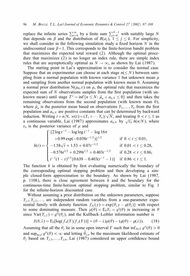
t=0 with suitably large Nthat depends on and the distribution of R(aj), 1 ≤ j ≤ k. For simplicity,we shall consider in the following simulation study a 0xed horizon N in theundiscounted case =1. This corresponds to the 0nite-horizon bandit problemthat maximizes the expected total reward (2). Although the optimal proce-dure that maximizes (2) is no longer an index rule, there are simple indexrules that are asymptotically optimal as N → ∞, as shown by Lai (1987).The starting point in Lai’s approximation is to consider the normal case.

Suppose that an experimenter can choose at each stage n(≤ N ) between sam-pling from a normal population with known variance 1 but unknown mean �and sampling from another normal population with known mean 0. Assuminga normal prior distribution N(�0; v) on �, the optimal rule that maximizes theexpected sum of N observations samples from the 0rst population (with un-known mean) until stage T ∗ = inf{n ≤ N : �n + an;N ≤ 0} and then takes theremaining observations from the second population (with known mean 0),where �n is the posterior mean based on observations Y1; : : : ; Yn from the 0rstpopulation and an;N are positive constants that can be determined by backwardinduction. Writing t=n=N; w(t)=(Y1+ · · ·Yn)=

√N , and treating 0¡t ≤ 1 as

a continuous variable, Lai (1987) approximates an;N by√vn h(n=N ), where

vn is the posterior variance of � and

h(t) =

{2 log t−1 − log log t−1 − log 16�

+0:99 exp(−0:038t−1=2)}1=2 if 0¡t ≤ 0:01;

−1:58√t + 1:53 + 0:07t−1=2 if 0:01¡t ≤ 0:28;

−0:576t3=2 + 0:299t1=2 + 0:403t−1=2 if 0:28¡t ≤ 0:86;

t−1(1− t)1=2{0:639− 0:403(t−1 − 1)} if 0:86¡t ≤ 1:

The function h is obtained by 0rst evaluating numerically the boundary ofthe corresponding optimal stopping problem and then developing a sim-ple closed-form approximation to the boundary. As shown by Lai (1987,p. 1108), there is close agreement between h and the boundary for thecontinuous-time 0nite-horizon optimal stopping problem, similar to Fig. 1for the in0nite-horizon discounted case.Without assuming a prior distribution on the unknown parameters, suppose

Yj;1; Yj;2; : : : ; are independent random variables from a one-parameter expo-nential family with density function f�j(y) = exp{�jy − g(�j)} with respectto some dominating measure. Then �(�) = E�Y1 = g′(�) is increasing in �since Var(Yj;1) = g′′(�j), and the Kullback–Leibler information number is

I(�; +) = E�[log(f�(Y )=f+(Y ))] = (�− +)�(�)− (g(�)− g(+)): (18)

Assuming that all the �j lie in some open interval 9 such that inf �∈9 g′′(�)¿ 0and sup�∈9 g′′(�)¡∞ and letting �j; n be the maximum likelihood estimate of�j based on Yj;1; : : : ; Yj;n, Lai (1987) considered an upper con0dence bound


for �(�j) of the form �(�∗j; n), where

� ∗j; n = inf{� ∈ 9: � ≥ �j; n; 2nI(�j; n; �) ≥ h2(n=N )}: (19)

Note that nI(�j; n; �0) is the generalized likelihood ratio statistic for testing�=�0, so the above upper con0dence bound adopts the usual construction ofcon0dence limits by inverting a generalized likelihood ratio test.De0ne the regret of an allocation rule at (�1; : : : ; �k) by

rN (�1; : : : ; �k) = N max1≤i≤k

�(�i)− E�1 ;:::;�k

{N−1∑t=0

R(Xt+1)

}: (20)

Note that the problem of maximizing the expected value of∑N−1

t=0 R(Xt+1)is equivalent to that of minimizing the regret. Lai and Robbins (1985) de-rived the following asymptotic lower bound for the regret rN (�1; : : : ; �k) ofuniformly good rules:

rN (�1; : : : ; �k) ≥ (logN )∑

j:�j¡� ∗

{�(� ∗)− �(�j)

I(�j; � ∗)+ o(1)

}; (21)

where � ∗ = max1≤i≤k �i, and a rule is said to be ‘uniformly good’ ifrN (�1; : : : ; �k) = O(logN ) for any 0xed (�1; : : : ; �k) ∈ 9k . Lai (1987) showedthat the preceding upper con0dence bound rule is uniformly good and attainsthe lower bound (21) not only at 0xed (�1; : : : ; �k) as N → ∞ (so that the ruleis asymptotically optimal from the frequentist viewpoint), but also uniformlyover a wide range of parameter con0gurations, which can be integrated toshow that the rule is asymptotically Bayes with respect to a large class ofprior distributions � for (�1; : : : ; �k).

This asymptotic theory for the 0nite-horizon undiscounted case is closelyrelated to the asymptotic theory, as the discount factor approaches 1, forthe discounted multi-armed bandit problem, in which the discounted regret ofan allocation rule at (�1; : : : ; �k) is de0ned by

r(�1; : : : ; �k) = E�1 ;:::;�k

[ ∞∑t=0

t{max1≤i≤k

�(�i)− R(Xt+1)}]

: (22)

Making use of (21) with N ∼ (1− )−1, Chang and Lai (1987) showed thatas → 1,

r(�1; : : : ; �k) ≥ |log(1− )|∑

j:�j¡� ∗

{�(� ∗)− �(�j)

I(�j; � ∗)+ o(1)

}(23)


for every rule that satis0es r(�′1; : : : ; �′k)=O(|log(1−)|) for all (�′1; : : : ; �′k) ∈

9k . They also showed that Gittins’ index rule and its approximation thatreplaces the Gittins indices by the simpler upper con0dence bounds (19)with h(n=N ) replaced by ({(1− )n}−1) attain the asymptotic lower bound(23) and are also asymptotically Bayes with respect to a large class of priors(not necessarily assuming independence among �1; : : : ; �k).While the regret of the preceding upper con0dence bound rule is of log-

arithmic order as N → ∞ in the 0nite-horizon case or as → 1 in the dis-counted case, the regret of the myopic rule that chooses the action with thelargest posterior mean reward (or the largest sample average reward withoutassuming a prior distribution on the unknown parameters) has regret of orderN (in the 0nite-horizon case) or order (1 − )−1 (in the discounted case);see Kumar (1985). Therefore the upper con0dence bound rule is consider-ably more eKcient than the myopic rule for large horizons N or for discountfactors approaching 1, showing the importance of active experimentation inthese cases. On the other hand, it is diKcult to improve on the myopic rulewhen N is moderate or small, or when there is substantial discounting, sincethe long-term bene0t of active experimentation to improve future performancecannot be realized when there is not much time left before the 0nal actionor when future values become insigni0cant after discounting.

Example 2. To illustrate this point, consider the case of Bernoulli banditswith k = 2 (arms) and a = b = 1 for the parameters of the prior Beta dis-tribution. The Bayesian myopic (BM) rule chooses the arm with the largerposterior mean at each stage, using randomization in the case of ties. Thefrequentist myopic (M) rule does not assume the Beta(1; 1) (or uniform)prior distribution for �1 or �2, and replaces the posterior mean in the BMrule by the sample mean. The upper con0dence bound (UCB) rule describedabove uses the upper con0dence bound (19) in lieu of the posterior mean.Table 2 gives the regret (20) of each rule at diIerent values of (�1; �2) forN = 20; 100; 300; 3000. Also given in Table 2 is the Bayes regret∫ 1

0

∫ 1

0rN (�1; �2) d�1 d�2 =N

∫ 1

0

∫ 1

0max(�1; �2) d�1 d�2 − R�

=2N=3− R� (24)

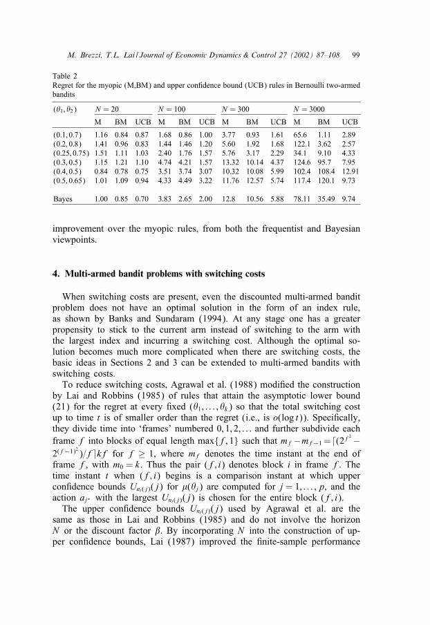
for each rule, where R� is the Bayes reward de0ned by (2) with uniform�. Each result in the table is based on 1000 simulations. Table 2 shows thatall three rules M, BM and UCB are nearly Bayes for N = 20, as they havesmall Bayes regret. While the regret function and the Bayes regret increaseslowly with N for the UCB rule, they grow much faster with N for themyopic rules M and BM. For N = 3000, the UCB rule that incorporates anappropriate amount of active experimentation in a simple way shows great


Table 2Regret for the myopic (M,BM) and upper con0dence bound (UCB) rules in Bernoulli two-armedbandits

(�1; �2) N = 20 N = 100 N = 300 N = 3000

M BM UCB M BM UCB M BM UCB M BM UCB

(0:1; 0:7) 1:16 0:84 0:87 1:68 0:86 1:00 3:77 0:93 1:61 65:6 1:11 2:89(0:2; 0:8) 1:41 0:96 0:83 1:44 1:46 1:20 5:60 1:92 1:68 122:1 3:62 2:57(0:25; 0:75) 1:51 1:11 1:03 2:40 1:76 1:57 5:76 3:17 2:29 34:1 9:10 4:33(0:3; 0:5) 1:15 1:21 1:10 4:74 4:21 1:57 13:32 10:14 4:37 124:6 95:7 7:95(0:4; 0:5) 0:84 0:78 0:75 3:51 3:74 3:07 10:32 10:08 5:99 102:4 108:4 12:91(0:5; 0:65) 1:01 1:09 0:94 4:33 4:49 3:22 11:76 12:57 5:74 117:4 120:1 9:73

Bayes 1:00 0:85 0:70 3:83 2:65 2:00 12:8 10:56 5:88 78:11 35:49 9:74

improvement over the myopic rules, from both the frequentist and Bayesianviewpoints.

4. Multi-armed bandit problems with switching costs

When switching costs are present, even the discounted multi-armed banditproblem does not have an optimal solution in the form of an index rule,as shown by Banks and Sundaram (1994). At any stage one has a greaterpropensity to stick to the current arm instead of switching to the arm withthe largest index and incurring a switching cost. Although the optimal so-lution becomes much more complicated when there are switching costs, thebasic ideas in Sections 2 and 3 can be extended to multi-armed bandits withswitching costs.To reduce switching costs, Agrawal et al. (1988) modi0ed the construction

by Lai and Robbins (1985) of rules that attain the asymptotic lower bound(21) for the regret at every 0xed (�1; : : : ; �k) so that the total switching costup to time t is of smaller order than the regret (i.e., is o(log t)). Speci0cally,they divide time into ‘frames’ numbered 0; 1; 2; : : : and further subdivide eachframe f into blocks of equal length max{f; 1} such that mf−mf−1=�(2f2 −2(f−1)2)=f�kf for f ≥ 1, where mf denotes the time instant at the end offrame f, with m0 = k. Thus the pair (f; i) denotes block i in frame f. Thetime instant t when (f; i) begins is a comparison instant at which uppercon0dence bounds Unt( j)(j) for �(�j) are computed for j = 1; : : : ; p, and theaction aj∗ with the largest Unt( j)(j) is chosen for the entire block (f; i).

The upper con0dence bounds Unt( j)(j) used by Agrawal et al. are thesame as those in Lai and Robbins (1985) and do not involve the horizonN or the discount factor . By incorporating N into the construction of up-per con0dence bounds, Lai (1987) improved the 0nite-sample performance


of the corresponding index-type rule in 0nite-horizon bandit problems with-out switching costs. In this connection, recall the role of N in h(n=N ) or ofc(=− log ) in (vj;n=c32(�j;n)) in determining the amount of active experi-mentation in (19) or (16). Moreover, the choice of blocks by Agrawal et al.(1988) does not involve N (or ). We can improve its performance by suit-ably incorporating this basic parameter into the de0nition of the blocks, as inthe following construction of nearly optimal allocation rules in the presenceof switching costs.

4.1. Normal two-armed bandits

To begin with, consider the 0nite-horizon bandit problem with k = 2normal arms, assuming common known variance 1 for each arm. For nota-tional simplicity let nt(1)=mt , nt(2)=nt , Yj=Yj;1, Zj=Yj;2, UY j=(Y1+· · ·+Yj)=j,UZj = (Z1 + · · ·+ Zj)=j. The generalized likelihood ratio (GLR) statistic ‘t fortesting H0 : EY1 = EZ1 based on Y1; : : : ; Ymt ; Z1; : : : ; Znt is given by

‘t =mtnt

2(mt + nt)( UYmt − UZnt)

2: (25)

Note that ‘t has the same form as the GLR statistic n UX2n=2 for testing H′

0: �=0based on i.i.d. normal X1; : : : ; Xn with mean � and variance 1, if we replacen by mtnt=(mt + nt) and UX n by UYmt − UZnt . As noted by Lai (1987), the uppercon0dence bound (19) in the UCB rule can be constructed by inverting aGLR test, and for the 0nite-horizon problem of choosing between a normalpopulation �1 with unknown mean � and another normal population �2

with known mean 0, a nearly optimal rule samples from the population withunknown mean until stage

T = inf{n ≤ N : 2nI( UX n; 0) ≥ h2(n=N )}= inf{n ≤ N : n UX

2n ≥ h2(n=N )}; (26)

and then samples the remaining N −T observations from �1 or �2 dependingon whether UX T ¿ 0 or UX T ¡ 0.Note that n UX n=w(n), where w(·) is a Wiener process with drift coeKcient

�. Letting � = EY1 − EZ1, Robbins and Siegmund (1974) have shown thatthe random sequences {mn( UYm − UZn)=(m + n)} and {w(mn=(m + n))} havethe same joint distribution for any sequence of integer pairs (m; n) which isnondecreasing in each coordinate. This suggests that in analogy with (26),after stage

�= inf{t: mt + nt ≤ N;

mtnt

mt + nt( UYmt − UZnt)

2 ≥ h2(

mtnt

(mt + nt)N

)};

(27)


we can stop sampling from Y or Z depending on whether UYm� ¡ UZn�or UZn� ¡ UYm� . Prior to stage �, we can use an adaptive sampling rule thatcarries out active experimentation with an apparently inferior population inblocks of consecutive time periods to reduce switching costs. This is the basicidea underlying the following sampling scheme.Take an even integer b (depending on the horizon N ) and partition time

into blocks so that the length of the jth block is bj −bj−1. In the 0rst block,sample b=2 observations 0rst from Y and then from Z with probability 1=2,and sample b=2 observations 0rst from Z and then from Y with probability1=2. For the jth block (j ≥ 2), we de0ne the leading population as thathaving the maximum of the two sample means at the end of the (j − 1)stblock. Sample the 0rst (bj − bj−1)=2 observations of the jth block from theleading population. Then switch to sampling from the other population untilstage

�j = inf{t: mt + nt ≤ bj; mtnt( UYmt − UZnt)2=(mt + nt)

≥ h2(mtnt=N (mt + nt))}: (28)

If the set in (28) is non-empty, stop experimentation and sample the remainingN − �j observations from Y (or Z) if UYm�j

¿ (or¡) UZn�j . In particular, if�j occurs at the time of switching with the leading population still havingthe larger sample mean, then no switching actually occurs as the apparentlyinferior population is eliminated from further sampling. If the set in (28) isempty, let �j = bj and note by induction that in this case we have sampledbj=2 observations from each population at the end of the jth block. If N =bJ for some integer J , the preceding de0nition applies to all J blocks. IfbJ−1 ¡N ¡bJ , we modify the de0nition of the J th block by proceeding asbefore until the N th (instead of the bJ th) observation. We shall call thisrule the block experimentation (BE) rule. It experiments with an apparentlyinferior population within blocks of consecutive times to reduce switchingcosts. The amount of experimentation is similar to that of the UCB rule, asillustrated in the following.

Example 3. The regret (20) of the BE rule that uses b = 10 to form theblocks is compared with that of the UCB rule and the frequentist myopic(M) rule described in Section 3, where the Bernoulli populations in Example2 are replaced by normal populations. Note that the 0rst block of the BE ruleconsists of the 0rst 10 stages, the second block consists of stages 11 through100, etc. Let � = EY1 − EZ1. Table 3 gives the results for various values of� and for N = 100 or 1000. They show that the BE rule has a somewhatlarger regret than the UCB rule but a substantially smaller regret than themyopic rule when N = 1000, although the regret of the myopic rule is onlyslightly larger than that of the BE rule when N =100. The expected number


Table 3Regret and expected number of switches for the myopic (M), upper con0dence bound (UCB)and block experimentation (BE) rules in normal two-armed bandits

� N = 100 N = 1000

Switch # Regret Switch # Regret

M UCB BE BE(2) M UCB BE BE(2) M UCB BE M UCB BE

1 2:31 5:01 3:90 5:82 12:35 4:12 8:72 7:30 2:89 8:60 3:90 95:5 6:6 10:20:8 2:38 5:94 3:78 6:22 10:97 4:85 9:17 7:59 2:41 11:1 3:83 82:3 7:7 11:50:6 2:55 6:98 3:69 6:58 11:46 5:06 9:44 8:21 2:43 14:1 3:74 118:2 8:8 14:30:4 2:65 9:33 3:36 7:22 11:35 6:08 10:07 7:85 2:71 17:8 4:03 104:3 10:5 16:10:2 2:82 10:55 3:23 7:87 8:33 5:75 7:08 6:49 2:79 28:6 4:42 72:5 19:4 28:40:1 2:85 11:79 3:12 7:87 4:96 3:93 4:25 3:55 3:08 34:9 4:32 41:8 22:5 27:0

of switches of the UCB rule, however, is considerably larger than that of theBE rule or the myopic rule.Unlike the rigid choice of frames and blocks in the rule of Agrawal et al.

(1988), the choice of b in the BE rule can depend on N and the switchingcost. In particular, it will be shown in Theorem 1 below that as N → ∞,by choosing b ∼ (logN )? with 1=2¡?¡ 1, the expected number of switchesconverges to 3.5 for 0xed � �= 0, while the regret of the BE rule is asymp-totically equivalent to that of the UCB rule. On the other hand, for moderatevalues of N and relatively small switching costs, it may be desirable to chooseb as small as 2. In particular, for the case N =100 in Table 3, the rule BE(2)

uses b=2. Its regret is closer to that of the UCB rule than that of BE (whichuses b= 10) while the expected number of switches increases substantially.

4.2. Extension to the exponential family and general k

The preceding block experimentation and sequential GLR testing ideas canbe readily generalized to k populations �1; : : : ; �k such that �i has densityfunction f�i(y)=exp{�iy− g(�i)} with respect to some common dominatingmeasure for i=1; : : : ; k. Let b be a positive integer divisible by k and partitiontime into frames such that the length of the jth frame is b for j = 1 and isbj−bj−1 for j ≥ 2. The jth frame is further subdivided into k blocks of equallength so that (j; i) refers to the ith block in frame j. Let (3(1); : : : ; 3(k)) be arandom permutation of (1; : : : ; k) (i.e., all k! permutations are equally likely).The block (1; i) in the 0rst frame is devoted to sampling from �3(i). For thejth frame (j ≥ 2), denote the population with the ith largest sample meanamong all populations not yet eliminated at the end of the (j−1)st frame by�3j(i). Let Ij denote the number of such populations and let i= 3j(i). Let �i∗

denote the population with the largest sample mean among all populations notyet eliminated at the end of the block (j; i − 1), where the end of the block


(j; 0) means the end of the frame j − 1. Let Yi;1; Yi;2; : : : denote successiveobservations from �i and UY i; t be the sample mean based on Yi;1; : : : ; Yi; t . Forthe block (j; i), which will be denoted by Bj; i (with 1 ≤ i ≤ Ij), we samplefrom �i until stage

�= inf

{t ∈ Bj; i: ‘( UY i∗ ; nt(i∗); UY i;nt(i); nt(i∗); nt(i))

≥ 12h2(

nt(i∗)nt(i)N [nt(i∗) + nt(i)]

)}; (29)

where � is de0ned as the largest number in Bj; i if the set in (29) is empty,and ‘( UY k;m; UY i;n;m; n) is the GLR statistic for testing H0: EYk = EYi basedon Yk;1; : : : ; Yk;m; Yi;1; : : : ; Yi;n and is given by (30) below. If the set in (29) isnon-empty, eliminate �i (or �i∗) from further sampling if UY i;n�(i) ¡ (or ¿)UY i∗ ; n�(i∗), and the remaining observations in the block (j; i) are sampled from�i∗ (or �i). Note that (29) reduces to (28) in the normal case, for which theGLR statistics are given by (25). For Ij ¡ i ≤ k, the block (j; i) is devotedto sampling from the population with the largest sample mean among allpopulations not yet eliminated at the end of block (j; Ij). We call this rulethe BE rule for the k-armed bandit problem.If N = bJ for some integer J , the preceding de0nition of the BE rule

applies to all J frames. If bJ−1 ¡N ¡bJ , we modify the de0nition of theJ th frame by proceeding as before until the N th observation. The follow-ing theorem, whose proof is given in the appendix, shows that the BE rulehas an asymptotically optimal regret and also gives the asymptotic behav-ior of its expected number of switches. As in Lai (1987), our analysis ofboundary crossing probabilities of GLR statistics in the proof of the theo-rem requires the regularity condition that �1; : : : ; �k all belong to an openinterval 9 = (�; �∗) such that −∞ ≤ �¡�∗ ≤ ∞, inf �−,¡�¡�∗+,g′′(�)¿ 0,sup�−,¡�¡�∗+, g

′′(�)¡∞ and g′′ is uniformly continuous on (� − ,; �∗ + ,)for some ,¿ 0. Note that this condition is satis0ed in the normal case with� = −∞ and �∗ = ∞. The maximum likelihood estimate of �(�i) based onYi;1; : : : ; Yi;m is �(�) ∨ ( UY i;m ∧ �(�∗)), where ∨ and ∧ denote maximum andminimum, respectively, and the GLR statistic for testing H0 :�(�k) = �(�i)based on Yk;1; : : : ; Yk;m; Yi;1; : : : ; Yi;n is

‘( UY k;m; UY i;n;m; n) =mL( UY k;m) + nL( UY i;n)

− (m+ n)L((m UY k;m + n UY i;n)=(m+ n)) (30)

with L(y)= L(�(�)∨ (y∧�(�∗))) and L(z)= z�−1(z)−g(�−1(z)), noting thatthe function �=g′ is continuous and increasing and therefore has an inverse.


Moreover, for this asymptotic theory, we can replace, as in Lai (1987), thespeci0c form of h in Section 3 by more general positive functions on (0; 1]such that for some B¿− 3=2,

h2(t) ∼ 2 log t−1 and h2(t)=2 ≥ log t−1 + B log log t−1 as t → 0:

(31)

Theorem 1. In the BE rule above; suppose b ∼ (logN )? for some 1=2¡?¡ 1and h : (0; 1] → (0;∞) satis.es (31) for some B¿− 3=2. Let I(�; +) denotethe Kullback–Leibler information number de.ned in (18). De.ne the re-gret rN (�1; : : : ; �k) of the BE rule by (20); and let sN (�1; : : : ; �k) denote itsexpected number of switches up to stage N . Let � ∗ =max1≤i≤k �i.(i) At every .xed (�1; : : : ; �k) ∈ 9k; as N → ∞;

rN (�1; : : : ; �k) ∼ (logN )∑

j:�j¡� ∗(�(� ∗)− �(�j))=I(�j; � ∗);

sN (�1; : : : ; �k) → 2k − k−1 if � ∗ = �i for only one i.(ii) Let #N (j) denote the expected number of observations from �j and

SN (j) denote the expected number of switches to and from �j up to stageN. Then as � ∗ − �j → 0 but N (� ∗ − �j)2 → ∞;

#N (j) ∼ (log[N (� ∗ − �j)2])=I(�j; � ∗);

SN (j) =O(max{1; | log(� ∗ − �j) | =log logN}):

Parts (i) and (ii) of Theorem 1 can be used to show that the Bayes re-gret

∫: : :∫rN (�1; : : : ; �k) d�(�1; : : : ; �k) is asymptotically minimal over a large

class of prior distributions �, as in Lai (1987).

4.3. Discounted bandit problems with switching costs

We can easily modify the BE rule for the in0nite-horizon discounted banditproblem with regret r(�1; : : : ; �k) de0ned by (22). Simply replace N in (29)by (1− )−1 and remove the upper bound J on the number of frames. Thismodi0ed rule will be denoted by BE. The analogue of sN (�1; : : : ; �k) in thediscounted problem is

s(�1; : : : ; �k) = E�1 ;:::;�k

[ ∞∑t=1

t1{a switch occurs at time t}

]:


Theorem 2. Suppose h : (0;∞) → (0;∞) satis.es (31) for some B¿ − 3=2and b ∼ | log(1− ) |? for some 1=2¡?¡ 1 in the BE rule. Then at every.xed (�1; : : : ; �k) ∈ 9k; as → 1;

r(�1; : : : ; �k) ∼ | log(1− ) |∑

j:�j¡� ∗(�(� ∗)− �(�j))=I(�j; � ∗);

s(�1; : : : ; �k) → 2k − k−1 if � ∗ = �i for only one i:

Moreover; the conclusion of Theorem 1(ii) also holds for the rule BE.

5. Conclusion

In Section 2, we provide closed-form approximations to Gittins indices sothat the optimal index rule can be easily implemented for discounted banditproblems. Although index rules are no longer optimal for 0nite-horizon (in-stead of discounted in0nite-horizon) multi-armed bandit problems, they areasymptotically optimal from both Bayesian and frequentist viewpoints forlarge horizons. They also perform well for small or moderate values of thehorizon N , for which even the myopic rule that does not incorporate activeexperimentation is shown to perform well in Section 3. When switching costsare present, even the discounted multi-armed bandit problem does not havean optimal solution in the form of an index rule, as shown by Banks andSundaram (1994). Nevertheless, Section 4 has shown how index rules can bemodi0ed by not switching within prespeci0ed blocks of time to come up withasymptotically optimal rules in the discounted or 0nite-horizon multi-armedbandit problem with switching costs.The incomplete learning theorem for discounted multi-armed bandits estab-

lished by Rothschild (1974), Banks and Sundaram (1992) and Brezzi and Lai(1999b) shows that in feedback control of a system with unknown parameters,the control objective may preclude full knowledge of the parameter valuesin the long run. However, one still needs suKcient information about theunknown parameters to come up with an appropriate action at every stage.A good control rule therefore introduces adjustments into the myopic ruleso that some active experimentation is used to generate information aboutthe unknown parameters. For discounted or 0nite-horizon multi-armed ban-dits, we have shown how such adjustments can be implemented by usingan index which replaces the sample estimates of the parameters by suitableupper con0dence bounds. In view of the duality between con0dence intervalsand hypothesis testing, we can also perform these adjustments by testing thehypothesis whether an apparently superior action is indeed superior. In par-ticular, we have used this hypothesis testing approach in Section 4 to addressthe long-standing problem of switching costs in multi-armed bandits.


Appendix.

Proof of Theorem 1. Consider the special case k=2, as the general case canbe treated by a similar argument. Without loss of generality, we shall assumethat �1 ¿�2. Let d= �1 − �2. In view of (31), we can make use of Lemma2:6 of Zhang (1992) on boundary crossing probabilities of GLR statistics(with a modi0cation of the statement to accommodate unequal sample sizesfrom the two populations but with essentially the same proof) to show thatas Nd2 → ∞ with O¡d= o((logN )1=2),

P{‘( UY 1; nt(1); UY 2; nt(2); nt(1); nt(2)) ≥ 12h2 (nt(1)nt(2)=N [nt(1) + nt(2)])

and UY 1; nt(1) ¡ UY 2; nt(2) for some t ≤ N}=O((Nd2)−1(logNd2)−B−1=2):

(A.1)

Consider the event F = {Population 1 is not eliminated at any stage t ≤ N},and let Fc denote its complement. Since Fc is a subset of the event in (A.1),P(Fc) =O((Nd2)−1) by (A.1). Note that

E{nN (2)1F} ≤ #N (2) ≤ NP(Fc) + E{nN (2)1F}=E{nN (2)1F}+O(d−2(logNd2)−B−1=2): (A.2)

Since B¿−3=2, it follows from (A.2) that #N (2)−E{nN (2)1F}=o(d−2logNd2).First consider the case of 0xed d¿ 0, as in part (i) of the theorem. By

standard large deviation bounds for sample means from an exponential family,there exists E¿ 0 such that

P{ UY 1;m ¡ UY 2; n}=O(e−Em + e−En) as m → ∞ and n → ∞: (A.3)

For the BE rule, nb(1)=nb(2)=b=2 ∼ (logN )?=2. On F ∩{ UY 1; nb(1) ¿ UY 2; nb(2)},the BE rule samples from �1 for stages nb(1) + 1; : : : ; nb(1) + (b2 − b)=2and then switches to sampling from �2 until the end of the second frameor the elimination of �2, whichever occurs sooner. Let �i = �(�i). SinceL′(y) = �−1(y), it follows that as m=n → ∞,

L(m�1 + n�2

m+ n

)= L(�1) +

nm+ n

(�2 − �1)�1 +O(( n

m

)2):

Since I(�2; �1)= (�2−�1)�2− (g(�2)−g(�1)) and L(�i)=�i�i −g(�i), it thenfollows that

mL(�1) + nL(�2)− (m+ n)L((m�1 + n�2)=(m+ n))

=n{L(�2)− L(�1)− (�2 − �1)�1 +O(n=m)}=n{I(�2; �1) +O(n=m)} (A.4)


as m=n → ∞. Noting that mn=(m + n) ∼ n as m=n → ∞ and using (31)and (A.4) together with the law of large numbers, it can be shown thatwith probability 1, �2 is eliminated at some stage t in frame 2 with nt(2) ∼(logN )=I(�2; �1). Uniform integrability arguments can then be used to showthat

E{nN (2)1F∩{ UY 1; nb(1)¿UY 2; nb(2)}} ∼ (logN )=I(�2; �1): (A.5)

Making use of exponential bounds for the large deviation probabilities ofsample means and noting that nN (2)¡b2 on the event that �2 is eliminatedin the second frame, we obtain that

E{nN (2)1F∩{ UY 1; nb(1)≤ UY 2; nb(2)}} ≤ b2e−Eb +O(Ne−Eb2); (A.6)

where the second summand on the right hand side simply bounds nN (2) byN . Since b2 ∼ (logN )2? and 2?¿ 1, it then follows that

E{nN (2)1F}= E{nN (2)1F∩{ UY 1; nb(1)¿UY 2; nb(2)}}+ o(1) ∼ (logN )=I(�2; �1):

The preceding proof also shows that on F ∩ { UY 1; nb(1) ¿ UY 2; nb(2)}, there aretwo switches in the second frame, to and from �2, with probability 1 asN → ∞. There is also one switch in the middle of the 0rst frame, and withprobability 1=2 one more switch at the end of the 0rst frame (when �1 ischosen at the beginning). Uniform integrability arguments and bounds of thetype in (A.6) then show that sN (�1; �2) → 3:5 in this case.We next consider the case d → 0 but Nd2 → ∞, as in part (ii) of the

theorem. In this case, (A.2) still holds and �2 is eliminated at some staget belonging to some frame j with nt(2) ∼ (logNd2)=I(�2; �1), with prob-ability approaching 1 as Nd2 → ∞. At the end of frame j − 1, the BErule has sampled bj−1=2 observations from each population on the eventF . Therefore, similar uniform integrability arguments can be used to showthat E{nN (2)1F} ∼ (logNd2)=I(�2; �1). Moreover, the expected number ofswitches is O(Jd), where bJd ¿ (1+o(1))(logNd2)=I(�2; �1)¿bJd−1=2. SinceI(�2; �1) ∼ d2g′′(�1)=2, we have

Jd log(logN )? = log(logN + logd2)− logd2 +O(log logN );

yielding ?Jd ∼ (−logd2)=(log logN ) +O(1).

Proof of Theorem 2. Take any a¿ 0 and choose a positive integer N (a) ∼a(1 − )−1. We can derive the desired conclusions as → 1 by applyingTheorem 1 to the horizon N (a) with a arbitrarily large.

References

Agrawal, R., Hegde, M.V., Teneketzis, D., 1988. Asymptotically eKcient adaptive allocationrules for the multiarmed bandit problem with switching costs. IEEE Transactions onAutomatic Control 33, 899–906.


Banks, J.S., Sundaram, R.K., 1992. Denumerable-narmed bandits. Econometrica 60, 1071–1096.Banks, J.S., Sundaram, R.K., 1994. Switching costs and the Gittins index. Econometrica 62,

687–694.Berry, D.A., 1972. A Bernoulli two-armed bandit. Annals of Mathematical Statistics 43,

871–897.Brezzi, M., Lai, T.L., 1999. Optimal stopping for Brownian motion in bandit problems and

sequential analysis, Working Paper, Department of Statistics, Stanford University.Brezzi, M., Lai, T.L., 2000. Incomplete learning from endogenous data in dynamic allocation.

Econometrica 68, 1511–1516.Chang, F., Lai, T.L., 1987. Optimal stopping and dynamic allocation. Advances of Applied

Probability 19, 829–853.ChernoI, H., Petkau, A.J., 1986. Numerical solutions for Bayes sequential decision problems.

SIAM Journal of Scienti0c and Statistical Computing 7, 46–59.Fabius, J., van Zwet, W.R., 1970. Some remarks on the two-armed bandit. Annals of

Mathematical Statistics 41, 1906–1916.Feldman, D., 1962. Contributions to the two-armed bandit problem. Annals of Mathematical

Statistics 33, 847–856.Gittins, J.C., 1979. Bandit processes and dynamic allocation indices. Journal of the Royal

Statistical Society, Series B 41, 148–177.Gittins, J.C., 1989. Multi-Armed Bandit Allocation Indices. Wiley, New York.Gittins, J.C., Jones, D.M., 1974. A dynamic allocation index for the sequential design of

experiments. In: Gani, J., Sarkadi, K., Vineze, I. (Eds.), Progress in Statistics. North-Holland,Amsterdam, pp. 241–266.

Jovanovich, B., 1979. Job-search and the theory of turnover. Journal of Political Economy 87,972–990.

Kumar, P.R., 1985. A survey of some results in stochastic adaptive control. SIAM Journal ofControl and Optimization 23, 329–380.

Lai, T.L., 1987. Adaptive treatment allocation and the multi-armed bandit problem. Annals ofStatistics 15, 1091–1114.

Lai, T.L., Robbins, H., 1985. Asymptotically eKcient adaptive allocation rules. Advances inApplied Mathematics 6, 4–22.

LeCam, L., 1953. On some asymptotic properties of maximum likelihood estimates and relatedBayes estimates. University of California Publications in Statistics 1, 277–330.

McLennan, A., 1984. Price disperson and incomplete learning in the long run. Journal ofEconomic Dynamics and Control 7, 331–347.

Mortensen, D., 1985. Job-search and labor market analysis. In: Ashenfelter, O., Layard, R.(Eds.),, Handbook of Labor Economics, Vol. 2. North Holland, Amsterdam, pp. 849–919.

Robbins, H., Siegmund, D., 1974. Sequential tests involving two populations. Journal of theAmerican Statistical Association 69, 132–139.

Rothschild, M., 1974. A two-armed bandit theory of market pricing. Journal of EconomicTheory 9, 185–202.

Whittle, P., 1980. Multi-armed bandits and the Gittins index. Journal of the Royal StatisticalSociety, Series B 42, 143–149.

Zhang, L., 1992. Asymptotically optimal sequential tests of linear hypotheses in multiparameterexponential families. Ph.D. Dissertation, Department of Statistics, Stanford University.

Documents

Optimal learning and experimentation in bandit …steele/Courses/900/Library/Bandits/...Journal of Economic Dynamics & Control 27 (2002) 87–108 Optimal learning and experimentation