Int. J. Production Economics 133 (2011) 451–457

Contents lists available at ScienceDirect

Int. J. Production Economics

0925-52

doi:10.1

n Corr

E-m

(Y. Mi

journal homepage: www.elsevier.com/locate/ijpe

Optimal inventory control of empty containers in inlandtransportation system

Won Young Yun a,n, Yu Mi Lee a, Yong Seok Choi b

a Department of Industrial Engineering, Pusan National University, Busan, Republic of Koreab Department of Logistics, Sunchon National University, Jeollanam-Do, Republic of Korea

a r t i c l e i n f o

Available online 8 July 2010

Keywords:

Empty containers

Inventory level

(s, S) inventory policy

Arena

OptQuests

73/$ - see front matter & 2010 Elsevier B.V. A

016/j.ijpe.2010.06.016

esponding author. Tel.: +82 51 510 2421; fax

ail addresses: wonyun@pusan.ac.kr (W. Youn

Lee), drasto@sunchon.ac.kr (Y. Seok Choi).

a b s t r a c t

In this paper, we deal with an inventory control problem of empty containers in an inland transportation

system. In inland container transportation, freights (containers) are transported between terminal and the

customer’s location by trucks, trains and barges. Empty containers are an important logistic resource and

shipping companies try to operate and manage empty containers efficiently. Because of the trade imbalance

between hub ports, empty containers should be periodically repositioned from surplus areas to shortage

areas. However, it is not easy to exactly forecast the demand of empty containers, and we therefore need to

build an efficient way to reposition the empty containers. In this paper, we consider a shortage area and

propose an efficient inventory policy to control empty containers. We assume that demands per unit time

are independent and identically distributed random variables. To satisfy the demand of empty containers,

we reposition empty containers from other hubs based on the (s, S) inventory policy, and also consider the

lease of empty containers with zero lead time. For the leased containers, we should return the number of

empty containers leased to the leaser after the specified period. For a given policy, simulation is used to

estimate the expected cost rate and we use the optimization tool, OptQuests in Arena to obtain the near

optimal (s, S) policy in numerical examples.

& 2010 Elsevier B.V. All rights reserved.

1. Introduction

The transportation demand of containers is rapidlyincreasing nowadays and the demand for empty containers isalso increasing accordingly. Because of the trade imbalance,empty containers should be repositioned between shortage andsurplus areas periodically and shipping companies need tohave an inventory control policy to reposition the emptycontainers. Shipping companies reposition empty containersbetween hub areas, ports and depots. Because it usually takes along time to reposition empty containers between hub areas andan efficient management of the empty containers is an importantfactor that can contribute to raising the productivity of shippingcompanies.

Crainic et al. (1993) dealt with the allocation problem of emptycontainers according to the dynamic and uncertainty of demand.Cheung and Chen (1998) considered how the dynamic containerallocation problem can be formulated as a two-stage stochasticnetwork model. They also studied optimization problems forrepositioning empty containers and determined how many leasedcontainers are needed at ports. Shen and Khoong (1995) proposed

ll rights reserved.

: +82 51 512 7603.

g Yun), ymlee@pusan.ac.kr

a network optimization model between ports and solved theproblem using A Mathematical Programming Language (AMPL).Lam et al. (2007) proposed dynamic and stochastic models for asimple two-port and two-voyage problem. Li et al. (2004), (2007)proposed a new (u, d) policy for the distribution problem of emptycontainers between ports.

In this paper, we consider a port area that needs more emptycontainers, known as a shortage area (for example, Busan, Korea).Suppose that we should prepare a suitable number of emptycontainers to satisfy the customer’s seasonally fluctuatingdemand. To satisfy the required number of empty containers,we can either reposition empty containers from the surplus areawith a long lead time or lease empty containers. Thus, weconsider the ordering (repositioning) and leasing policy underprobabilistic demand and supply, with high and low demandseasons for the demand of empty containers. Holding, leasing andordering costs are considered and we obtain optimum inventorypolicies to minimize the expected cost rate (long-run average costper unit time) by an ARENA simulation.

2. Inventory control model

Fig. 1 shows an inland transportation network. Shippingcompanies store empty containers in depots, provide the empty

Lease Company

TerminalDepot Terminal

CustomersFull container movement

Empty container movement

Fig. 1. Inland transportation network.

Fig. 2. Ordering and leasing policy using the (s, S) ordering policy.

W. Young Yun et al. / Int. J. Production Economics 133 (2011) 451–457452

containers for transportation of freights between terminal andcustomer locations, and sometimes lease empty containers if theyneed more empty containers immediately. In this paper, we considera hub area, in which more empty containers are needed because thedemand of empty containers is greater than the supply. To solve theimbalance problem, we should periodically reposition emptycontainers from surplus areas to a shortage area. In this paper, aninventory control problem of empty containers under probabilisticdemand is studied under the following assumptions.

Assumptions

(1)

40 ft dry containers are considered. (2) There are two seasons: low and high demand seasons. (3) Demand and supply of empty containers per week are

independent and identically distributed random variables.

(4) (s, S) ordering policy is used. (5) There is a type of lease with zero lead time. (6) The lead time of repositioning is constant.

Notation

S1 order-up-to level at low demand seasons1 order point at low demand seasonS2 order-up-to level at high demand seasons2 order point at high demand seasonLT lead time of repositioningDi customer’s demand in period i

Oi order amount in period i

Li lease amount in period i

Hi stock level in period i

Ni net stock at the beginning in period i

Ii inventory level during the lead time in period i

Vi return amount from customers in period i

Cf fixed-ordering costCo ordering cost on each unitCl leasing cost on each unitCn inventory holding cost on each unitTCi total cost in period i

W. Young Yun et al. / Int. J. Production Economics 133 (2011) 451–457 453

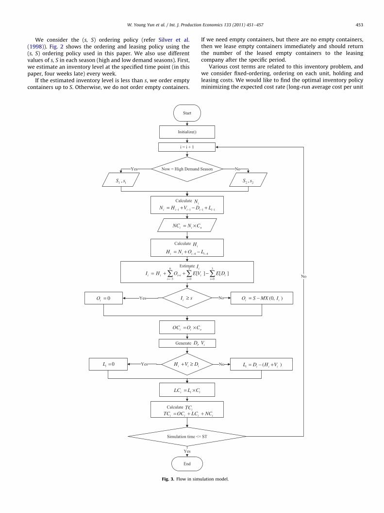
We consider the (s, S) ordering policy (refer Silver et al.(1998)). Fig. 2 shows the ordering and leasing policy using the(s, S) ordering policy used in this paper. We also use differentvalues of s, S in each season (high and low demand seasons). First,we estimate an inventory level at the specified time point (in thispaper, four weeks late) every week.

If the estimated inventory level is less than s, we order emptycontainers up to S. Otherwise, we do not order empty containers.

Fig. 3. Flow in sim

If we need empty containers, but there are no empty containers,then we lease empty containers immediately and should returnthe number of the leased empty containers to the leasingcompany after the specific period.

Various cost terms are related to this inventory problem, andwe consider fixed-ordering, ordering on each unit, holding andleasing costs. We would like to find the optimal inventory policyminimizing the expected cost rate (long-run average cost per unit

ulation model.

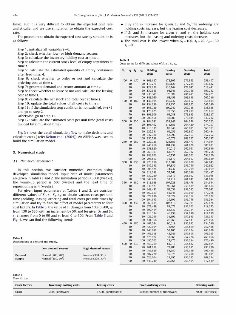
Table 3Costs terms for different values of S1, s1, S2, s2.

S1 s1 S2 s2 Holdingcosts

Leasingcosts

Orderingcosts

Totalcosts

100 0 130 0 103,147 173,307 276,953 553,407

10 20 110,275 146,123 277,224 533,622

30 40 122,652 116,744 279,045 518,441

50 60 132,915 93,541 282,756 509,212

70 80 139,380 76,685 288,209 504,275

90 100 143,060 68,459 293,698 505,216

150 0 180 0 143,994 146,237 268,662 558,894

10 20 154,289 124,235 268,825 547,349

30 40 168,729 100,240 269,718 538,688

50 60 178,625 78,955 271,287 528,867

70 80 191,306 63,088 273,933 528,327

90 100 203,468 48,589 278,144 530,202

200 0 230 0 184,341 138,147 264,278 586,765

10 20 198,402 111,885 264,420 574,707

30 40 213,339 89,949 265,015 568,303

50 60 225,581 69,056 265,847 560,484

70 80 237,388 52,696 267,167 557,252

90 100 250,788 40,072 269,327 560,187

250 0 280 0 227,725 124,885 261,473 614,084

W. Young Yun et al. / Int. J. Production Economics 133 (2011) 451–457454

time). But it is very difficult to obtain the expected cost rateanalytically, and we use simulation to obtain the expected costrate.

The procedure to obtain the expected cost rate by simulation isas follows:

Step 1: initialize all variables t¼0.Step 2: check whether low- or high-demand season.Step 3: calculate the inventory holding cost at time t.Step 4: calculate the current stock level of empty containers attime t.Step 5: calculate the estimated quantity of empty containersafter lead time, 4.Step 6: check whether to order or not and calculate theordering cost at time t.Step 7: generate demand and return amount at time t.Step 8: check whether to lease or not and calculate the leasingcost at time t.Step 9: calculate the net stock and total cost at time t.Step 10: update the total values of all costs to time t.Step 11: if the simulation stop condition is not satisfied, t¼t+1and go to step 2.Otherwise, go to step 12.Step 12: calculate the estimated costs per unit time (total costsdivided by simulation time).

Fig. 3 shows the detail simulation flow to make decisions andcalculate costs ( refer Kelton et al. (2004)). An ARENA was used tobuild the simulation model.

10 20 240,766 104,237 261,628 606,631

30 40 258,820 80,016 262,061 600,896

50 60 269,303 63,573 262,382 595,258

70 80 283,101 46,757 263,301 593,160

90 100 298,853 36,179 264,507 599,539

300 0 330 0 270,656 112,387 259,600 642,643

10 20 285,333 97,832 259,756 642,922

30 40 305,524 74,747 259,789 640,059

50 60 318,338 57,763 260,396 636,497

70 80 332,220 39,816 261,062 633,098

90 100 348,207 31,717 261,747 641,672

350 0 380 0 318,688 107,528 258,478 684,694

10 20 336,523 90,661 258,489 685,674

30 40 349,483 69,053 258,545 677,082

50 60 362,013 51,245 259,000 672,258

70 80 379,736 37,624 259,362 676,722

90 100 394,633 29,192 259,758 683,584

400 0 430 0 363,019 102,416 257,393 722,828

10 20 377,449 84,672 257,153 719,275

30 40 397,464 62,837 257,324 717,625

50 60 413,334 46,739 257,716 717,789

70 80 429,266 34,192 257,935 721,393

90 100 441,356 26,269 257,443 726,068

3. Numerical study

3.1. Numerical experiment

In this section, we consider numerical examples usingdeveloped simulation model. Input data of model parametersare given in Tables 1 and 2. The simulation period is 5000 (weeks),the warm-up period is 500 (weeks) and the lead time ofrepositioning is 4 (weeks).

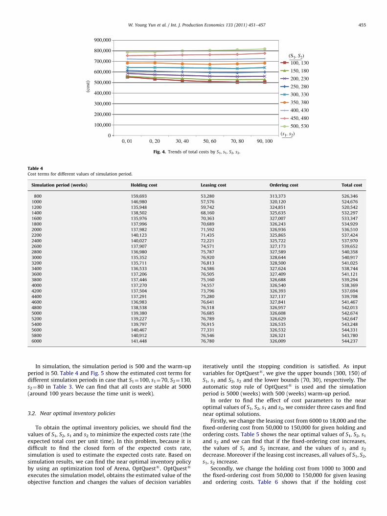
For given input parameters at Tables 1 and 2, we considerdifferent values of S1, s1, S2, s2, to obtain various costs per unittime (holding, leasing, ordering and total costs per unit time) bysimulation and try to find the effect of model parameters to fourcost factors. In Table 3, the value of S1 changes from 100 to 500, S2

from 130 to 530 with an increment by 50, and for given S1 and S2,s1 changes from 0 to 90 and s2 from 0 to 100. From Table 3 andFig. 4, we can find the following trends:

Table 2Costs factors.

Costs factors Inventory holding costs Leasing costs

Costs 2000 (unit/week) 12,000 (unit/mont

Table 1Distributions of demand and supply.

Low demand season High demand season

Demand Normal (200, 202) Normal (300, 302)

Supply Normal (150, 202) Normal (220, 302)

�

h)

4

5

If s1 and s2 increase for given S1 and S2, the ordering andholding costs increase, but the leasing cost decreases.

� If S1 and S2 increase for given s1 and s2, the holding cost

increases, but the leasing and ordering costs decrease.

� The total cost is the lowest when S1¼100, s1¼70, S2¼130,

s2¼80.

Fixed-ordering costs Ordering costs

50,000 (number of times/week) 4000 (unit/week)

50 0 480 0 407,344 90,619 256,833 754,796

10 20 422,064 78,464 256,899 757,428

30 40 446,080 58,165 256,724 760,970

50 60 463,018 43,541 256,806 763,365

70 80 475,477 33,363 257,226 766,066

90 100 495,702 23,475 257,314 776,490

00 0 530 0 450,769 81,013 255,822 787,604

10 20 461,658 72,483 256,095 790,236

30 40 489,616 53,680 256,169 799,466

50 60 507,720 39,075 256,290 803,085

70 80 523,604 29,395 256,235 809,234

90 100 540,730 20,365 256,454 817,549

900,000

(cos

t)

800,000

100, 130(S1, S2)

700,000

150, 180600,000200, 230

500,000250, 280

400,000 300, 330

350, 380300,000400, 430

200,000450, 480

500, 530100,000

0 (s1, s2)

0, 01 0, 20 30, 40 50, 60 70, 80 90, 100

Fig. 4. Trends of total costs by S1, s1, S2, s2.

Table 4Cost terms for different values of simulation period.

Simulation period (weeks) Holding cost Leasing cost Ordering cost Total cost

800 159,693 53,280 313,373 526,346

1000 146,980 57,576 320,120 524,676

1200 135,948 59,742 324,851 520,542

1400 138,502 68,160 325,635 532,297

1600 135,976 70,363 327,007 533,347

1800 137,996 70,689 326,243 534,929

2000 137,982 71,592 326,936 536,510

2200 140,123 71,435 325,865 537,424

2400 140,027 72,221 325,722 537,970

2600 137,907 74,571 327,173 539,652

2800 136,980 75,787 327,589 540,358

3000 135,352 76,920 328,644 540,917

3200 135,711 76,813 328,500 541,025

3400 136,533 74,586 327,624 538,744

3600 137,206 76,505 327,409 541,121

3800 137,446 75,160 326,688 539,294

4000 137,270 74,557 326,540 538,369

4200 137,504 73,796 326,393 537,694

4400 137,291 75,280 327,137 539,708

4600 136,983 76,641 327,841 541,467

4800 138,538 76,518 326,957 542,013

5000 139,380 76,685 326,608 542,674

5200 139,227 76,789 326,629 542,647

5400 139,797 76,915 326,535 543,248

5600 140,467 77,331 326,532 544,331

5800 140,912 76,546 326,321 543,780

6000 141,448 76,780 326,009 544,237

W. Young Yun et al. / Int. J. Production Economics 133 (2011) 451–457 455

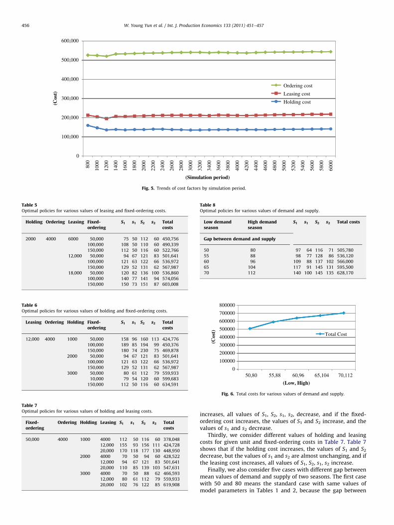
In simulation, the simulation period is 500 and the warm-upperiod is 50. Table 4 and Fig. 5 show the estimated cost terms fordifferent simulation periods in case that S1¼100, s1¼70, S2¼130,

s2¼80 in Table 3. We can find that all costs are stable at 5000(around 100 years because the time unit is week).

3.2. Near optimal inventory policies

To obtain the optimal inventory policies, we should find thevalues of S1, S2, s1 and s2 to minimize the expected costs rate (theexpected total cost per unit time). In this problem, because it isdifficult to find the closed form of the expected costs rate,simulation is used to estimate the expected costs rate. Based onsimulation results, we can find the near optimal inventory policyby using an optimization tool of Arena, OptQuests. OptQuests

executes the simulation model, obtains the estimated value of theobjective function and changes the values of decision variables

iteratively until the stopping condition is satisfied. As inputvariables for OptQuests, we give the upper bounds (300, 150) ofS1, s1 and S2, s2 and the lower bounds (70, 30), respectively. Theautomatic stop rule of OptQuests is used and the simulationperiod is 5000 (weeks) with 500 (weeks) warm-up period.

In order to find the effect of cost parameters to the nearoptimal values of S1, S2, s1 and s2, we consider three cases and findnear optimal solutions.

Firstly, we change the leasing cost from 6000 to 18,000 and thefixed-ordering cost from 50,000 to 150,000 for given holding andordering costs. Table 5 shows the near optimal values of S1, S2, s1

and s2 and we can find that if the fixed-ordering cost increases,the values of S1 and S2 increase, and the values of s1 and s2

decrease. Moreover if the leasing cost increases, all values of S1, S2,s1, s2 increase.

Secondly, we change the holding cost from 1000 to 3000 andthe fixed-ordering cost from 50,000 to 150,000 for given leasingand ordering costs. Table 6 shows that if the holding cost

600,000

(Cos

t)500,000

400,000

300,000

Ordering cost

Leasing cost

Holding cost

200,000

100,000

0

(Simulation period)

800

1000

1200

1400

1600

1800

2000

2200

2400

2600

2800

3000

3200

3400

3600

3800

4000

4200

4400

4600

4800

5000

5200

5400

5600

5800

6000

Fig. 5. Trends of cost factors by simulation period.

Table 5Optimal policies for various values of leasing and fixed-ordering costs.

Holding Ordering Leasing Fixed-ordering

S1 s1 S2 s2 Totalcosts

2000 4000 6000 50,000 75 50 112 60 450,756

100,000 108 50 110 60 490,339

150,000 112 50 116 60 522,766

12,000 50,000 94 67 121 83 501,641

100,000 121 63 122 66 536,972

150,000 129 52 131 62 567,987

18,000 50,000 120 82 136 100 536,860

100,000 140 77 141 94 574,056

150,000 150 73 151 87 603,008

Table 6Optimal policies for various values of holding and fixed-ordering costs.

Leasing Ordering Holding Fixed-ordering

S1 s1 S2 s2 Totalcosts

12,000 4000 1000 50,000 158 96 160 113 424,776

100,000 189 85 194 99 450,376

150,000 180 74 230 75 469,878

2000 50,000 94 67 121 83 501,641

100,000 121 63 122 66 536,972

150,000 129 52 131 62 567,987

3000 50,000 80 61 112 79 559,933

10,000 79 54 120 60 599,683

150,000 112 50 116 60 634,591

Table 7Optimal policies for various values of holding and leasing costs.

Fixed-ordering

Ordering Holding Leasing S1 s1 S2 s2 Totalcosts

50,000 4000 1000 4000 112 50 116 60 378,048

12,000 155 93 156 111 424,728

20,000 170 118 177 130 448,950

2000 4000 70 50 94 60 428,522

12,000 94 67 121 83 501,641

20,000 110 85 139 103 547,631

3000 4000 70 50 88 62 466,593

12,000 80 61 112 79 559,933

20,000 102 76 122 85 619,908

Table 8Optimal policies for various values of demand and supply.

Low demandseason

High demandseason

S1 s1 S2 s2 Total costs

Gap between demand and supply

50 80 97 64 116 71 505,780

55 88 98 77 128 86 536,120

60 96 109 88 137 102 566,000

65 104 117 91 145 131 595,500

70 112 140 100 145 135 628,170

800000

(Cos

t)

700000

600000

500000

400000 Total Cost

300000

200000

100000

0

(Low, High)

50,80 55,88 60,96 65,104 70,112

Fig. 6. Total costs for various values of demand and supply.

W. Young Yun et al. / Int. J. Production Economics 133 (2011) 451–457456

increases, all values of S1, S2, s1, s2, decrease, and if the fixed-ordering cost increases, the values of S1 and S2 increase, and thevalues of s1 and s2 decrease.

Thirdly, we consider different values of holding and leasingcosts for given unit and fixed-ordering costs in Table 7. Table 7shows that if the holding cost increases, the values of S1 and S2

decrease, but the values of s1 and s2 are almost unchanging, and ifthe leasing cost increases, all values of S1, S2, s1, s2 increase.

Finally, we also consider five cases with different gap betweenmean values of demand and supply of two seasons. The first casewith 50 and 80 means the standard case with same values ofmodel parameters in Tables 1 and 2, because the gap between

W. Young Yun et al. / Int. J. Production Economics 133 (2011) 451–457 457

mean demand and supply is 50 and 80 for two seasons. For otherfour cases, we make the gap larger by increasing the meandemands of two seasons.

Table 8 and Fig. 6 show that if the gap between demand andsupply increases in each season, then all values of S1, s1 and, S2, s2

increase and the total cost also increase.

4. Conclusions

In this paper, we considered an inventory control problem ofempty containers. For probabilistic demand of empty containerswith low and high seasons in a hub area, we used the (s, S)inventory policy to order empty containers from other hub areas.While there is a lead time for repositioning, we can lease emptycontainers immediately. Holding, leasing and ordering costs areconsidered and the expected cost rate (long-run average cost perunit time) is an optimization criterion. Simulation is used toobtain the expected cost rate and some numerical examples arestudied. For given values of model parameters, OptQuests isused to find the near optimal inventory policy based onsimulation results.

For further studies, we will consider coordinate inventoryproblems of empty containers in multi-depot cases and in thispaper, an independent and identical distribution is assumed forprobabilistic demand, but more complicate stochastic processescan also be used and similar inventory problems can be studied.

Acknowledgements

‘‘This work was supported by the Grant of the Korean Ministryof Education, Science and Technology (The Regional Core ResearchProgram/Institute of Logistics Information Technology)’’ (TheRegional Research Universities Program/Research Center forLogistics Information Technology).

References

Cheung, R.K., Chen, C.Y., 1998. A two-stage stochastic network model and solutionmethods for the dynamic empty container allocation problem. TransportationScience 32, 142–166.

Crainic, T.G., Gedreau, M., Dejax, P., 1993. Dynamic and stochastic models for theallocation of empty containers. Operations Research Society of America 41,102–125.

Kelton, W.D., Sadowski, R.P., Sturrock, D.T., 2004. Simulation with Arena, third ed.McGraw-Hill.

Li, J.A., Liu, K., Leung, Stephen C.H., Lai, K.K., 2004. Empty container management ina port with long-run average criterion. Mathematical and Computer Modeling40, 85–100.

Li, J.A., Leung, Stephen C.H., Wu, Y., Liu, K., 2007. Allocation of empty containersbetween multi-ports. European Journal of Operational Research 182, 400–412.

Lam, S.W., Lee, L.H., Tang, L.C., 2007. An approximate dynamic programmingapproach for the empty container allocation problem. Transportation ResearchPart C 15, 265–277.

Silver, E.A., Pyke, D.F., Peterson, R., 1998. Inventory Management and ProductionPlanning and Scheduling, third ed. John Wiley & Sons.

Shen, W.S., Khoong, C.M., 1995. A DSS for empty container distribution planning.Decision Support Systems 15, 75–82.