OPTIMAL INEQUALITIES IN PROBABILITY THEORY: A · PDF fileThe idea that optimization methods and duality theory can be used to address moment-type inequalities in probability ﬁrst

SIAM J. OPTIM. c© 2005 Society for Industrial and Applied MathematicsVol. 15, No. 3, pp. 780–804

OPTIMAL INEQUALITIES IN PROBABILITY THEORY: A CONVEXOPTIMIZATION APPROACH∗

DIMITRIS BERTSIMAS† AND IOANA POPESCU‡

Abstract. We propose a semidefinite optimization approach to the problem of deriving tightmoment inequalities for P (X ∈ S), for a set S defined by polynomial inequalities and a random vectorX defined on Ω ⊆ Rn that has a given collection of up to kth-order moments. In the univariate case,we provide optimal bounds on P (X ∈ S), when the first k moments of X are given, as the solutionof a semidefinite optimization problem in k + 1 dimensions. In the multivariate case, if the sets Sand Ω are given by polynomial inequalities, we obtain an improving sequence of bounds by solvingsemidefinite optimization problems of polynomial size in n, for fixed k.

We characterize the complexity of the problem of deriving tight moment inequalities. We showthat it is NP-hard to find tight bounds for k ≥ 4 and Ω = Rn and for k ≥ 2 and Ω = Rn

+, when thedata in the problem is rational. For k = 1 and Ω = Rn

+ we show that we can find tight upper boundsby solving n convex optimization problems when the set S is convex, and we provide a polynomialtime algorithm when S and Ω are unions of convex sets, over which linear functions can be optimizedefficiently. For the case k = 2 and Ω = Rn, we present an efficient algorithm for finding tight boundswhen S is a union of convex sets, over which convex quadratic functions can be optimized efficiently.

Key words. probability bounds, Chebyshev inequalities, semidefinite optimization, convexoptimization

AMS subject classifications. 60E15, 90C22, 90C25

DOI. 10.1137/S1052623401399903

1. Introduction. The problem of deriving bounds on the probability that acertain random variable belongs in a given set, given information on some of itsmoments, has a very rich and interesting history, which is very much connected withthe development of probability theory in the twentieth century. The inequalities due toMarkov, Chebyshev, and Chernoff are some of the classical and widely used results ofmodern probability theory. Natural questions, however, that arise are the following:

1. Are such bounds “best possible”; i.e., do there exist distributions that matchthem?

2. Can such bounds be generalized in multivariate settings, and in what circum-stances can they be explicitly and/or algorithmically computed?

3. Is there a general theory based on optimization methods to address in a unifiedmanner moment-inequality problems in probability theory?

In this paper, we formulate the problem of obtaining best possible bounds as anoptimization problem and use modern optimization theory, in particular convex andsemidefinite programming, to give concrete answers to the questions above. We firstintroduce some notation. Let κ = (k1, . . . , kn)′ with kj ∈ Z+ nonnegative integers.We use the notation σκ = σk1,...,kn

and Jk = κ = (k1, . . . , kn)′ | k1+· · ·+kn ≤ k, kj ∈Z+, j = 1, . . . , n. We next introduce the notion of a feasible moment sequence.

∗Received by the editors December 18, 2001; accepted for publication (in revised form) June 29,2004; published electronically April 8, 2005.

http://www.siam.org/journals/siopt/15-3/39990.html†Sloan School of Management, Rm. E53-363, Massachusetts Institute of Technology, Cambridge,

MA 02139 ([email protected]). The research of this author was partially supported by NSF grantDMI-9610486 and the MIT-Singapore Alliance.

‡INSEAD, Fontainebleau Cedex 77305, France ([email protected]).

780

OPTIMAL PROBABILITY BOUNDS 781

Definition 1.1. A sequence σ = (σκ, κ ∈ Jk) is a feasible (n, k,Ω)-momentvector (or sequence), if there is a random vector X = (X1, . . . , Xn)′ defined on Ω ⊆ Rn

endowed with its Borel sigma algebra of events, whose moments are given by σ, thatis, σκ = σk1,...,kn = E

[Xk1

1 · · ·Xknn

]for all κ ∈ Jk. We say that any such random

variable X has a σ-feasible distribution and denote this as X ∼ σ.Throughout the paper, the underlying probability space is implicitly assumed

to be Ω ⊆ Rn endowed with its Borel sigma algebra of events. We denote byM = M(n, k,Ω) the set of feasible (n, k,Ω)-moment vectors. For the univariatecase (n = 1), the problem of deciding if σ = (M1,M2, . . . ,Mk)

′ is a feasible (1, k,Ω)-moment vector is the classical moment problem. This problem has been completelycharacterized by necessary and sufficient conditions by Stieltjes [43], [44] in 1894-95,who adopts the “moment” terminology from mechanics (see also Karlin and Shapley[18], Akhiezer [1], Siu, Sengupta, and Lind [38], and Kemperman [21]). For univariate,nonnegative random variables (Ω = R+), these conditions can be written as Rk 0and Rk−1 0, where for any integer l ≥ 0 we define

R2l =

⎛⎜⎜⎜⎝

1 M1 . . . Ml

M1 M2 . . . Ml+1

......

. . ....

Ml Ml+1 . . . M2l

⎞⎟⎟⎟⎠ , R2l+1 =

⎛⎜⎜⎜⎝

M1 M2 . . . Ml+1

M2 M3 . . . Ml+2

......

. . ....

Ml+1 Ml+2 . . . M2l+1

⎞⎟⎟⎟⎠ .

For univariate random variables with Ω = R, the necessary and sufficient condi-tion (given by Hamburger [12], [13] in 1920-21) for a vector σ = (M1,M2, . . . ,Mk)

′ tobe a feasible (1, k,R)-moment sequence is that R2 k

2 0 . In the multivariate case,

the formulation of the problem can be traced back to Haviland [14], [15] in 1935-36(see also Godwin [10]). To date, the sufficiency part of the moment problem has notbeen completely resolved in the multivariate case, although substantial progress hasbeen made in the last decade by Schmudgen [37] and Putinar [34].

Suppose that σ is a feasible moment sequence and X has a σ-feasible distribution.We now define the central problem that this paper addresses.

The (n, k, Ω)-bound problem. Given a sequence σκ, κ = (k1, k2, . . . , kn)′ ∈ Jkof up to kth-order moments

σκ = E[Xk1

1 Xk22 · · ·Xkn

n

], κ ∈ Jk

of a random vector X = (X1, X2, . . . , Xn)′ on Ω ⊆ Rn endowed with its Borel sigmaalgebra, find the “best possible” or “tight” upper and lower bounds on P (X ∈ S), formeasurable events S ⊆ Ω.

The term “best possible” or “tight” upper (and by analogy lower) bound aboveis defined as follows.

Definition 1.2. We say that γ is a tight upper bound on P (X ∈ S) if γ =supX∼σ P (X ∈ S).

Note that a bound can be tight without necessarily being exactly achievable (i.e.,there is a random variable X(0) ∼ σ for which P (X(0) ∈ S) = γ), but only asymptot-ically (i.e., there exists a sequence of random variables X(i)i≥1 such that X(i) ∼ σand limi→∞ P (X(i) ∈ S) = γ).

The well-known inequalities due to Markov, Chebyshev, and Chernoff, which arewidely used if we know the first moment, the first two moments, and all moments(i.e., the generating function) of a random variable, respectively, are feasible butnot necessarily optimal solutions to the (n, k,Ω)-bound problem; i.e., they are notnecessarily tight bounds.

782 DIMITRIS BERTSIMAS AND IOANA POPESCU

Literature and historical perspective. The history of the developments inthe area of (n, k,Ω)-bound problems, sometimes referred to as generalized Chebyshevinequalities, can be traced back to the work of Gauss, Cauchy, Chebyshev, Markov,etc., and has witnessed an unexpected evolution. The problem of finding boundson univariate distributions under moment constraints was proposed and formulatedwithout proof initially by Chebyshev [6] in 1874 and resolved ten years later by hisstudent Markov [25] in his Ph.D. thesis, using continued fractions techniques. In the1950s and 1960s there was a revival of the interest in this area, that resulted in alarge literature on Chebyshev systems and inequalities. Surveys of early literaturecan be found in Shohat and Tamarkin [40] and Godwin [9], [10]. A detailed, unifiedaccount of the evolution of Chebyshev systems is given by Karlin and Studden [19] intheir 1966 monograph (see in particular Chapters 12 and 13 that deal with (n, k,Ω)-type bounds). In particular, they summarize the results of Marshall and Olkin [27],[28] who computed tight, explicit bounds on probabilities given first- and second-order moments (the (n, 2,Ω) problem in our context), thus generalizing Chebyshev’sinequality to a multivariate setting.

Not for the first time in its history, and in the words of Shohat and Tamarkinin1943 [40, p. 10], “the problem of moments lay dormant for more than 20 years.” Itrevived briefly in the 1980s, with the book on probability inequalities and multivariatedistributions of Tong [45] in 1980, who also published a monograph on probabilityinequalities in 1984. The latter notably contains, among others, a generalization ofMarkov’s inequality for multivariate tails, due to Marshall [26]. A volume in Momentsin Mathematics edited by Landau in 1987 includes a background survey by the sameauthor [23], as well as relevant papers of Kemperman [22] and Diaconis [7].

The idea that optimization methods and duality theory can be used to addressmoment-type inequalities in probability first appeared in 1960, and is due indepen-dently and simultaneously to Isii [16] and Karlin (lecture notes at Stanford, see [19,p. 472]), who showed via strong duality results that certain types of Chebyshev in-equalities for univariate random variables are sharp. Isii [17] extended these dualityresults for random vectors on complete regular spaces. Thirty two years after Isii’s [17]original multivariate proof, Smith [42] rederived the duality result and proposed newinteresting applications in decision analysis, dynamic programming, statistics, and fi-nance. Shapiro [39] provided a rigorous discussion of necessary topological conditionsfor strong duality to hold, in that sense relaxing the compactness assumptions under-lying Isii’s proof. For an in-depth account of strong duality and sensitivity analysisfor a general class of semi-infinite programming problems see Bonnans and Shapiro[3, Section 5.4].

For a broader investigation of the optimization framework underlying this typeof problem, we refer the interested reader to Borwein and Lewis [4], [5] who providean in-depth analysis of partially finite convex programming.

Despite its long and scattered history, the common belief among researchers isstill that “the theory [of moment problems] is not up to the demands of applications”(Diaconis [7, p. 129]). The same author suggested that one of the reasons couldbe the high complexity of the problem: “numerical determination . . . is feasible for asmall number of moments, but appears to be quite difficult in general cases.” Anotherreason, as identified by Kemperman (see [22, p. 20]), is the lack of a general algorithmicapproach:

“. . . a deep study of algorithms has been rare so far in the theoryof moments, except for certain very specific practical applications, for


instance, to crystallography, chemistry and tomography. No doubt,there is a considerable need for developing reasonably good numer-ical procedures for handling the great variety of moment problemswhich do arise in pure and applied mathematics and in the sciencesin general . . . .”

In an attempt to address Kemperman’s criticism, Smith [42] actually introduced acomputational procedure for the (n, k,Rn)-bound problem, although he does not referto it in this way. Unfortunately, the procedure is far from a formal algorithm, as thereis no proof of convergence, and no investigation (theoretical or experimental) of itsefficiency. It is fair to say that a thorough understanding of the algorithmic aspectsand the complexity of the (n, k,Ω)-bound problem is still lacking.

Yet another criticism brought by Smith is the lack of simple, closed-form solutionsfor the (n, k,Rn)-bound problem: “the bounds given by Chebyshev’s inequalities . . .are quite loose. The more general versions are rarely used because of the lack ofsimple closed-form expressions for the bounds” (see [42, p. 808]).

Goals and contributions. The previous discussion motivates our desire in thepresent paper to understand the complexity of deriving tight moment inequalities,search for efficient algorithms in a general framework, and, when possible, derivesimple closed-form bounds. In particular, we characterize which classes of (n, k,Ω)-bound problems are efficiently solvable and which are NP-hard.

Let us remark that the theory of polynomial solvability and NP-hardness assumea rational computational model. For this reason, as far as complexity results areconcerned, we work under the assumption that the problem data is rational; i.e.,moments are rational numbers and the sets Ω and S are specified in terms of rationalnumbers. Specifically, they are defined by semialgebraic sets (i.e., sets that are definedin terms of polynomial inequalities), whose parameters are rational numbers. Inaddition, throughout the paper we refer to an efficient, or polynomial time algorithmwhen it takes polynomial time in the problem data and log(1/ε), and it computes abound within ε of the tight bound for all ε > 0.

More concretely, the contributions and structure of the paper are as follows.

1. In section 3, we investigate in detail the univariate case, i.e., the (1, k,Ω)-bound problem for Ω = R,R+. We show that tight bounds can be computed effi-ciently by solving a single semidefinite optimization problem. We also derive tightbounds for tail probability events in closed form, when up to three moments are given.For k = 1, we recover the Markov inequality, which also shows that the Markov boundis tight. For k = 2, we recover a strict improvement of the Chebyshev inequality thatretains the simplicity of the bound. This inequality dates back at least to Uspensky’sbook (see [46, p. 198]) from 1937, who proposed it as an exercise. Despite its simplic-ity, the bound has been strangely ignored in the recent literature and textbooks. Fork = 3, we present closed-form tight bounds that appear to be new.

2. In section 4, we generalize the results of the previous section to the multivari-ate (n, k,Ω)-bound problem. For a fairly general class of semialgebraic sets S and Ω(not necessarily convex), we propose a sequence of increasingly stronger, asymptoti-cally exact upper bounds by solving semidefinite optimization problems of polynomialsize in n. This includes the case when Ω is a bounded polyhedron, or a semialgebraicset such that Ω ⊆ x ∈ Rn | x′x ≤ M2 and M is known a priori. The proposed ap-proach gives rise to a family of semidefinite relaxations whose size is polynomial in n.We also show that the (n, k,Rn

+), (n, k,Rn)-bound problems for k ≥ 2, respectivelyk ≥ 4, are NP-hard.


Table 1

The landscape of the (n, k,Ω)-problem (BP refers to the current paper).

n = 1 nS convex set S union of convex sets

k = 1 Theorem 3.3 Theorem 5.1 Algorithm A, section 5.2Markov [25] Marshall [26], BP BP

k = 2 Theorem 3.3 Theorem 6.1 Algorithm B, section 6.2Chebyshev [6] Marshall and Olkin [27] BP

k Theorem 3.2: SDP Theorem 4.3: SDP; Propositions 4.5, 4.6: NP-hardnessBP BP

3. In section 5, we address the (n, 1,Ω) problem. We show that if the set S inthe definition of the (n, 1,Rn)-bound problem is convex, we find best possible boundsfor P (X ∈ S) explicitly as a solution of n convex optimization problems. We alsoprovide a polynomial time algorithm to solve the (n, 1,Ω) problem, when the setsS and Ω are the union of disjoint convex sets, over which a linear function can beefficiently optimized. These bounds represent natural extensions of the inequalitiesdue to Markov in the univariate case, and Marshall [26] for multivariate tails.

4. In section 6, we first review the work of Marshall and Olkin [27] who showedthat the (n, 2,Rn)-bound problem can be solved as a single convex optimization prob-lem. We provide an efficient algorithm for the case when S is a union of disjoint convexsets, over which a convex quadratic function can be optimized efficiently.

Table 1 summarizes the contributions of the paper to the (n, k,Ω)-bound problem.

2. Primal and dual formulations of the (n, k, Ω)-bound problem. In thissection, we formulate the (n, k,Ω)-upper bound problem as an optimization problem,where Ω ∈ Rn is the domain of the random variables under consideration. We examinethe corresponding dual problem and present weak and strong duality results thatpermit us to develop algorithms for the problem. The same approach and resultsapply to the (n, k,Ω)-lower bound problem.

We use the notation zκ = zk11 · · · zkn

n , where z = (z1, . . . , zn)′ and κ = (k1, . . . , kn)′,kj ∈ Z+. Recall that Jk = κ = (k1, . . . , kn)′ | k1 + · · · + kn ≤ k, kj ∈ Z+, j =1, . . . , n. The (n, k,Ω)-upper bound problem can be formulated as the following op-timization problem:

ZP = maxµ

∫S

1 dµ

subject to

∫Ω

zκdµ = σκ ∀κ ∈ Jk.(2.1)

The variable of the infinite-dimensional optimization problem (2.1) is the probabilitymeasure µ (so implicitly dµ(z) ≥ 0 a.e.). We assume that σ0,...,0 = 1, correspondingto the probability mass constraint. If problem (2.1) is feasible, then σ is a feasiblemoment sequence, and any feasible distribution µ is a σ-feasible distribution. Thefeasibility problem is exactly the classical multidimensional moment problem.

In the spirit of linear programming duality theory, we associate a dual variableyκ = yk1,...,kn

with each equality constraint of the primal and we obtain

ZD = miny∈R|Jk|

∑κ∈Jk

yκσκ

subject to g(z) =∑κ∈Jk

yκzκ ≥ 1 ∀z ∈ S,

(2.2)


g(z) =∑κ∈Jk

yκzκ ≥ 0∀z ∈ Ω.

While in principle the dual constraints may only need to hold a.e., this is equiv-alent to solving (2.2) since polynomial positivity holds a.e. if and only if it holdseverywhere.

In general, the optimum in problem (2.1) may not be achievable. Wheneverthe primal optimum is achieved, we call the corresponding distribution an extremaldistribution. In the case when only (say upper) bounds on moments σκ are known,then in the dual problem we add the inequalities yκ ≥ 0. Thus, our results (specificallyTheorems 3.2 and 4.3 below) regarding efficient solvability of the underlying problemgeneralize to the case when only bounds on moments are known. We next establishweak duality.

Theorem 2.1 (weak duality). ZP ≤ ZD.Proof. Let µ be a primal feasible solution and let yκ, κ ∈ Jk, be a dual feasible

solution. From dual feasibility we have that for all z ∈ Ω, g(z) =∑

κ∈Jkyκz

κ ≥ χS(z),where χS(z) = 1 if z ∈ S, and 0, otherwise. Then

ZP =

∫S

1dµ =

∫Ω

χS(z)dµ ≤∫

Ω

g(z)dµ =∑κ∈Jk

yκ

∫Ω

zκdµ =∑κ∈Jk

yκσκ = ZD.

Theorem 2.1 indicates that by solving the dual problem (2.2) we obtain an upperbound on the primal objective, and hence on the probability we are trying to estimate.If the moment vector σ is an interior point of the set of feasible moment vectors, thedual bound turns out to be tight. This strong duality result follows from a univariateresult due to Karlin and Isii in 1960 (see Karlin and Studden [19, p. 472]), andgeneralized by Isii in 1963 [17] for random vectors defined on complete regular spaces.Shapiro [39, Proposition 3.4] provides a modern proof based on conic linear duality,under a general topological structure. The following theorem is a consequence of theirwork, and holds for general distributions of X (discrete, continuous, with or withoutatoms, etc.) over a metric space Ω endowed with its Borel sigma algebra.

Theorem 2.2 (strong duality). If the moment vector σ is an interior point ofthe set M of feasible moment vectors, then ZP = ZD.

If the dual is unbounded, it is immediate from weak duality that the multidi-mensional moment problem is infeasible. On the other hand, if the common optimalvalue is finite, then the set of dual optimal solutions is nonempty and bounded (seeIsii [17], Kemperman [20], or Shapiro [39]). Furthermore, if σ is a boundary pointof M, then it can be shown that the σ-feasible distributions are concentrated on asubset Ω0 of Ω, and strong duality holds provided we relax the dual to Ω0 (see Isii[17, p. 190] or Smith [42, p. 824]). These authors also prove that it is equivalent tooptimize only over discrete distributions that are concentrated on m+2 points, wherem is the number of moment constraints.

In the univariate case, Isii [16] proves that if σ is a boundary point of M, thenexactly one σ-feasible distribution exists. Kemperman [20] proves that for almostevery σ (with respect to the Lebesgue measure) such that the dual is finite, the dualsolution is unique (see also Shapiro [39, Proposition 3.5]). In Chapter 5.4 of theirrecent book, Bonnans and Shapiro [3] provide necessary and sufficient conditions forthe uniqueness of the optimal distribution, as well as sensitivity results.

If strong duality holds, then by optimizing over problem (2.2) we obtain a tightbound on P (X ∈ S). On the other hand, it is worthwhile to remark that under


certain technical conditions (see Grotschel, Lovasz, and Schrijver [11]) solving problem(2.2) is equivalent to solving the corresponding separation problem, which amountsto verifying polynomial positivity conditions over S and Ω.

3. The (1, k, Ω)-bound problem. In this section, we restrict our attention tounivariate random variables. Given the first k moments M1, . . . ,Mk (we let M0 = 1)of a real random variable X with domain Ω ⊆ R, we are interested in deriving tightbounds on P (X ∈ S). This is the (1, k,Ω)-bound problem. Our main result in thissection is that tight bounds can be derived as a solution to a single semidefiniteoptimization problem. We also derive closed-form tight bounds when up to the firstthree moments are given.

3.1. Tight bounds as semidefinite optimization problems. In the one-dimensional case, problem (2.2) becomes

minimizek∑

r=0

yrMr

subject to

k∑r=0

yrxr ≥ 1 ∀x ∈ S,

k∑r=0

yrxr ≥ 0 ∀x ∈ Ω.

(3.1)

Problem (3.1) naturally leads us to investigate conditions for polynomials to be non-negative. When S and Ω are intervals on the real line, we show in the next propo-sition that the feasible region of problem (3.1) can be expressed using semidefiniteconstraints. Semidefinite optimization problems are efficiently solvable using inte-rior point methods. For a review of semidefinite optimization see Wolkowicz, Saigal,and Vandenberghe [47]. The results and the proofs in the following proposition areinspired by Nesterov [31] (see also Ben-Tal and Nemirovski [2, pp. 140–142]).

Proposition 3.1. (a) The polynomial g(x) =∑2k

r=0 yrxr satisfies g(x) ≥ 0 for

all x ∈ R if and only if there exists a positive semidefinite matrix X = [xij ]i,j=0,...,k,such that

yr =∑

i,j:i+j=r

xij , r = 0, . . . , 2k, X 0.(3.2)

(b) The polynomial g(x) =∑k

r=0 yrxr satisfies g(x) ≥ 0 for all x ≥ 0 if and only

if there exists a positive semidefinite matrix X = [xij ]i,j=0,...,k, such that

0 =∑

i,j:i+j=2l−1

xij , l = 1, . . . , k,

yl =∑

i,j:i+j=2l

xij , l = 0, . . . , k,

X 0.

(3.3)


(c) The polynomial g(x) =∑k

r=0 yrxr satisfies g(x) ≥ 0 for all x ∈ [0, a] if and

only if there exists a positive semidefinite matrix X = [xij ]i,j=0,...,k, such that

0 =∑

i,j:i+j=2l−1

xij , l = 1, . . . , k,

l∑r=0

yr

(k − r

l − r

)ar =

∑i,j:i+j=2l

xij , l = 0, . . . , k,

X 0.

(3.4)

(d) The polynomial g(x) =∑k

r=0 yrxr satisfies g(x) ≥ 0 for all x ∈ [a,∞) if and


0 =∑

i,j:i+j=2l−1

xij , l = 1, . . . , k,

k∑r=l

yr

(r

l

)ar−l =

∑i,j:i+j=2l

xij , l = 0, . . . , k,

X 0.

(3.5)

(e) The polynomial g(x) =∑k

r=0 yrxr satisfies g(x) ≥ 0 for all x ∈ (−∞, a] if

and only if there exists a positive semidefinite matrix X = [xij ]i,j=0,...,k, such that

0 =∑

i,j:i+j=2l−1

xij , l = 1, . . . , k,

(−1)lk∑

r=l

yr

(r

l

)ar−l =

∑i,j:i+j=2l

xij , l = 0, . . . , k,

X 0.

(3.6)

(f) The polynomial g(x) =∑k

r=0 yrxr satisfies g(x) ≥ 0 for all x ∈ [a, b] if and


0 =∑

i,j:i+j=2l−1

xij , l = 1, . . . , k,

l∑m=0

k+m−l∑r=m

yr

(r

m

)(k − r

l −m

)ar−mbm =

∑i,j:i+j=2l

xij , l = 0, . . . , k,

X 0.

(3.7)

Proof.(a) Suppose (3.2) holds. Let x(k) = (1, x, x2, . . . , xk)′. Then

g(x) =2k∑r=0

∑i+j=r

xijxr

=

k∑i=0

k∑j=0

xijxixj

= x′(k)Xx(k)

≥ 0,


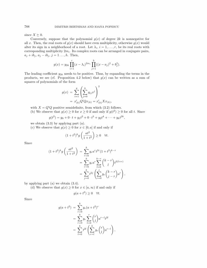
since X 0.Conversely, suppose that the polynomial g(x) of degree 2k is nonnegative for

all x. Then, the real roots of g(x) should have even multiplicity, otherwise g(x) wouldalter its sign in a neighborhood of a root. Let λi, i = 1, . . . , r, be its real roots withcorresponding multiplicity 2mi. Its complex roots can be arranged in conjugate pairs,aj + ibj , aj − ibj , j = 1 . . . , h. Then,

g(x) = y2k

r∏i=1

(x− λi)2mi

h∏j=1

((x− aj)2 + b2j ).

The leading coefficient y2k needs to be positive. Thus, by expanding the terms in theproducts, we see (cf. Proposition 4.2 below) that g(x) can be written as a sum ofsquares of polynomials of the form

g(x) =

p∑i=1

⎛⎝ k∑

j=0

qijxj

⎞⎠

2

= x′(k)Q

′Qx(k) = x′(k)Xx(k),

with X = Q′Q positive semidefinite, from which (3.2) follows.(b) We observe that g(x) ≥ 0 for x ≥ 0 if and only if g(t2) ≥ 0 for all t. Since

g(t2) = y0 + 0 · t + y1t2 + 0 · t3 + y2t

4 + · · · + ykt2k,

we obtain (3.3) by applying part (a).(c) We observe that g(x) ≥ 0 for x ∈ [0, a] if and only if

(1 + t2)kg

(at2

1 + t2

)≥ 0 ∀t.

Since

(1 + t2)kg

(at2

1 + t2

)=

k∑r=0

yrart2r(1 + t2)k−r

=

k∑r=0

yrark−r∑l=0

(k − r

l

)t2(l+r)

=

k∑j=0

t2j

(j∑

r=0

yr

(k − r

j − r

)ar

),

by applying part (a) we obtain (3.4).(d) We observe that g(x) ≥ 0 for x ∈ [a,∞) if and only if

g(a + t2) ≥ 0 ∀t.Since

g(a + t2) =

k∑r=0

yr(a + t2)r

=

k∑r=0

yr

r∑l=0

(r

l

)ar−lt2l

=

k∑l=0

t2l

(k∑

r=l

yr

(r

l

)ar−l

),


by applying part (a) we obtain (3.5).

(e) We observe that g(x) ≥ 0 for x ∈ (−∞, a] if and only if

g(a− t2) ≥ 0 ∀t.

Since

g(a− t2) =

k∑r=0

yr(a− t2)r

=

k∑r=0

yr

r∑l=0

(r

l

)ar−l(−t2)l

=

k∑l=0

t2l

((−1)l

k∑r=l

yr

(r

l

)ar−l

),


(f) We observe that g(x) ≥ 0 for x ∈ [a, b] if and only if

(1 + t2)kg

(a + (b− a)

t2

1 + t2

)≥ 0 ∀t.

Since

(1 + t2)kg

(a + (b− a)

t2

1 + t2

)=

k∑r=0

yr(a + bt2)r(1 + t2)k−r

=

k∑r=0

yr

r∑m=0

(r

m

)ar−mbmt2m

k−r∑j=0

(k − r

j

)t2j

=

k∑l=0

t2l

(l∑

m=0

k+m−l∑r=m

yr

(r

m

)(k − r

l −m

)ar−mbm

),


We next show that problem (3.1) can be written as a semidefinite optimizationproblem. Corresponding formulations, which we omit here for the sake of conciseness,can be obtained similarly for the problem of establishing lower bounds, i.e., problem(2.1) in which we replace maximization by minimization.

Theorem 3.2. Given the first k moments (M1, . . . ,Mk) (we let M0 = 1) of arandom variable X defined on Ω we obtain the following tight upper bounds.

(a) If Ω = R+, the tight upper bound on P (X ≥ a) is given as the solution of the


semidefinite optimization problem

minimizek∑

r=0

yrMr

subject to 0 =∑

i,j:i+j=2l−1

xij , l = 1, . . . , k,

(y0 − 1) +

k∑r=1

yrar = x00,

k∑r=l

yr

(r

l

)ar−l =

∑i,j:i+j=2l

xij , l = 1, . . . , k,

0 =∑

i,j:i+j=2l−1

zij , l = 1, . . . , k,

l∑r=0

yr

(k − r

l − r

)ar =

∑i,j:i+j=2l

zij , l = 0, . . . , k,

X,Z 0.

(3.8)

If Ω = R, then the last equation in (3.8) should be replaced by

(−1)lk∑

r=l

yr

(r

l

)ar−l =

∑i,j:i+j=2l

zij , l = 0, . . . , k.

(b) If Ω = R+, the tight upper bound on P (a ≤ X ≤ b) is given as the solutionof the semidefinite optimization problem

minimize

k∑r=0

yrMr

subject to 0 =∑

i,j:i+j=2l−1

xij , l = 1, . . . , k,

l∑m=0

k+m−l∑r=m

yr

(r

m

)(k − r

l −m

)ar−mbm=

(k

l

)+

∑i,j:i+j=2l

xij , l = 0, . . . , k,

0 =∑

i,j:i+j=2l−1

zij , l = 1, . . . , k,

yl =∑

i,j:i+j=2l

zij , l = 0, . . . , k,

X,Z 0.

(3.9)

If Ω = R, then the last equation in (3.9) should be replaced by

(−1)lk∑

r=l

yr

(r

l

)ar−l =

∑i,j:i+j=2l

zij , l = 0, . . . , k,


and the following equations added:

0 =∑

i,j:i+j=2l−1

uij , l = 1, . . . , k,

k∑r=l

yr

(r

l

)br−l =

∑i,j:i+j=2l

uij , l = 0, . . . , k,

U 0.

Proof.(a) The feasible region of problem (3.1) for S = [a,∞) and Ω = R+ becomes

g(x) =

k∑r=0

yrxr ≥ 1 ∀x ∈ [a,∞) and g(x) ≥ 0 ∀x ∈ [0, a).

By applying Proposition 3.1(c), (d) we obtain (3.8). If Ω = R, we apply Proposi-tion 3.1(d), (e).

(b) The feasible region of problem (3.1) for S = [a, b] and Ω = R+ becomes

g(x) =

k∑r=0

yrxr ≥ 1 ∀x ∈ [a, b] and g(x) ≥ 0 ∀x ∈ [0,∞).

By applying Proposition 3.1(b), (f) we obtain (3.9). If Ω = R, we apply Proposi-tion 3.1(d), (e), (f).

3.2. Closed-form bounds. In this section, we present closed-form bounds whenmoments up to third order are given. We define the squared coefficient of variation

C2M =

M2−M21

M21

, and the third-order coefficient of variation D2M =

M1M3−M22

M41

. Let

δ > 0.Theorem 3.3. The following bounds in Table 2 are tight for k = 1, 2, 3.The bounds marked with an asterisk (∗) assume that δ < 1 (the other case is

trivial). The following definitions are used:

f1(C2M , D2

M , δ) =

⎧⎪⎪⎪⎨⎪⎪⎪⎩

min

(C2

M

C2M + δ2

,1

1 + δ· D2

M

D2M + (C2

M − δ)2

), if δ > C2

M ,

1

1 + δ· D2

M + (1 + δ)(C2M − δ)

D2M + (1 + C2

M )(C2M − δ)

, if δ ≤ C2M ,

f2(C2M , D2

M , δ) = 1 − (C2M + δ)3

(D2M + (C2

M + 1)(C2M + δ))(D2

M + (C2M + δ)2)

,

f3(C2M , D2

M , δ) = min

(1, 1 + 33 D2

M + C4M − δ2

4 + 3(1 + 3δ2) + 2(1 + 3δ2)32

).

The proof of the theorem is given in Popescu [33].

4. The (n, k, Ω)-bound problem: Semidefinite formulations and com-plexity. In this section, we generalize the results of the previous section to the mul-tivariate case by investigating the (n, k,Ω)-bound problem. For a fairly general class


Table 2

Tight bounds for the (1, k,Ω)-problem for k ≤ 3.

(k, Ω) P (X > (1 + δ)M1) P (X < (1 − δ)M1) P (|X −M1| > δM1)

(1,R+) 11+δ

1∗ 1∗

(2,R)C2

M

C2M

+δ2C2

M

C2M

+δ2min

(1,

C2Mδ2

)

(3,R+) f1(C2M , D2

M , δ) f2(C2M , D2

M , δ)∗ f3(C2M , D2

M , δ)∗

of semialgebraic sets S and Ω, i.e., sets that are given as intersections of inequali-ties involving polynomials, we propose a sequence of increasingly stronger, asymp-totically exact upper bounds by solving semidefinite optimization problems. Thisincludes the case when Ω is a bounded polyhedron, or a semialgebraic set such thatΩ ⊆ x ∈ Rn | x′x ≤ M2 and M is known a priori. Note that it is not necessaryfor the sets S and Ω to be convex. We expect that in general an exact semidefiniteformulation, if it exists, may be exponential in n even for fixed k. This fact shouldnot be surprising, given that in section 4.2 we prove that it is NP-hard to find bestpossible bounds for the (n, k,Rn)-bound problem for k ≥ 4. We also show that it isNP-hard to find best possible bounds for the (n, k,Rn

+)-bound problem for k ≥ 2.

4.1. Semidefinite programming formulations. The approach we follow inthis section has its origin in the work of Shor [41]. Recently it has been used byLasserre [24] and Parrilo [32] to provide semidefinite relaxations for discrete opti-mization and nonconvex optimization problems.

In dimension n = 1, we have seen in the proof of Proposition 3.1 that a polynomialin one dimension is nonnegative if and only if it can be written as a sum of squares ofpolynomials. Clearly, in multiple dimensions if a polynomial can be written as a sum ofsquares of other polynomials, then it is nonnegative. Hilbert, in a nonconstructive way,has shown that it is possible for a polynomial in higher dimensions to be nonnegativewithout being a sum of squares. Motzkin (see Reznick [35]) has shown that thepolynomial

M(x, y, z) = x4y2 + x2y4 + z6 − 3x2y2z2

is nonnegative without being a sum of squares of polynomials. The connection betweennonnegative polynomials and sum of squares representations has a long history thatis nicely outlined in Reznick [35]. In this paper we will rely on the following theoremdue to Putinar [34].

Theorem 4.1 (Putinar [34]). Suppose that the set

K = x ∈ Rn | gi(x) ≥ 0, i ∈ I

is compact and there exists a polynomial h(x) of the form

h(x) = h0(x) +∑i∈I

hi(x)gi(x),

such that x ∈ Rn | h(x) ≥ 0 is compact and hi(x), i ∈ I ∪ 0 are polynomials thathave a sum of squares representation. Then, for any polynomial g(x) that is strictly


positive for all x ∈ K, there exist pi(x), i ∈ I ∪ 0, that are sums of squares suchthat

g(x) = p0(x) +∑i∈I

pi(x)gi(x).(4.1)

Putinar [34] shows that the conditions for Theorem 4.1 to hold are relatively mild. Inparticular, examples of sets K that satisfy the conditions of Theorem 4.1 include thefollowing.

(a) One of the defining inequalities of K represents a compact set x ∈ Rn |gl(x) ≥ 0. This is the case, for example, when gl(x) = c − (x − x0)

′Q(x − x0), andQ 0.

(b) K is a bounded polyhedron.(c) K is compact, and there is a bound M a priori known such that K ⊆ x ∈

Rn | x′x ≤ M2.While Theorem 4.1 guarantees the existence of the representation in (4.1), it does

not give any information on the degree of the polynomials pi(x). From Theorem 4.1 itis natural to investigate when a polynomial is a sum of squares. Let x(d) be the vectorof all monomials in the variables x1, . . . , xn of degree d and below. For example, forn = 2, d = 2,

x(2) = (1, x1, x2, x21, x1x2, x

22)

′.

There are a =(n+dd

)such monomials.

Proposition 4.2. The polynomial f(x) of degree 2d has a sum of squares de-composition if and only if there exists a positive semidefinite matrix Q for whichf(x) = x

′(d)Qx(d).

Proof. To simplify notation, let x = x(d) throughout the proof. An arbitrarypolynomial of degree 2d can be written as f(x) = x

′Qx for some a× a matrix Q (thematrix Q is not unique, however). If Q 0, then Q = HH ′ for some H, and thus,

f(x) = x′HH ′

x =

a∑i=1

(H ′x)2i .

Since (H ′x)i is a polynomial, we have expressed f(x) as a sum of squares of the

polynomials (H ′x)i.

Conversely, suppose that f(x) has a sum of squares decomposition

f(x) =

l∑i=1

hi(x)2 =

l∑i=1

(h′ix)2 =

l∑i=1

x′(hih

′i)x = x

′

(l∑

i=1

(hih′i)

)x = x

′Qx,

where hi is the vector of coefficients of the polynomial hi(x). Since Q =∑l

i=1(hih′i)

0, the proposition follows.Therefore, if the sets Ω and S satisfy the conditions of Theorem 4.1, by applying

Proposition 4.2, we can express problem (2.2) as a semidefinite optimization problem.Suppose that the sets Ω and S are semialgebraic sets, given by

Ω =

x ∈ Rn | ωi(x) =

∑κ∈Jl

ωiκx

κ ≥ 0, i = 1, . . . , r

,

S =

x ∈ Rn | si(x) =

∑κ∈Jt

siκxκ ≥ 0, i = 1, . . . ,m

,


where ωiκ, siκ ∈ R, that is Ω and S are defined by polynomial inequalities. We use

the notation δκ,0 = 1 if κ = 0, and zero, otherwise.Theorem 4.3. If the sets Ω and S satisfy the conditions of Theorem 4.1, then

for every ε > 0 there exists a nonnegative integer d ∈ Z+ (representing the degree ofthe polynomials in (4.1)), such that the objective function value ZD in problem (2.2)satisfies |ZD − ZD(d)| ≤ ε, where ZD(d) is the value of the following semidefiniteprogram:

ZD(d) = min∑κ∈Jk

yκσκ

subject to yκ − δκ,0 = q0κ +

m∑i=1

∑η ∈Jd, θ ∈Jt

η+θ = κ

qiηsiθ ∀κ ∈ Jk,

0 = q0κ +

m∑i=1

∑η ∈Jd, θ ∈Jt

η + θ = κ

qiηsiθ ∀κ ∈ Js+d \ Jk,

yκ = p0κ +

r∑i=1

∑η ∈Jd, θ ∈Jl

η + θ = κ

piηωiθ ∀κ ∈ Jk,

0 = p0κ +

r∑i=1

∑η ∈Jd, θ ∈Jl

η + θ = κ

piηωiθ ∀κ ∈ Jl+d \ Jk,

qiκ =∑

η,θ∈Jd ,η+θ=κ

qiη,θ ∀κ ∈ Jd, i = 0, 1, . . . ,m,

piκ =∑

η,θ∈Jd, η+θ=κ

piη,θ ∀κ ∈ Jd, i = 0, 1, . . . ,m,

Qi = [qiη,θ]η,θ∈Jd 0, i = 0, 1, . . . , r,

P i = [piη,θ]η,θ∈Jd 0, i = 0, 1, . . . ,m.

(4.2)

Proof. We first remark that the value of the dual problem (2.2) equals that of thefollowing strict inequality formulation:

ZD = infy∈R|Jk|

∑κ∈Jk

yκσκ

subject to g(x) =∑κ∈Jk

yκxκ > 1 ∀x ∈ S,

g(x) =∑κ∈Jk

yκxκ > 0 ∀x ∈ Ω.

(4.3)

This problem may not admit an optimal solution. However, for any ε > 0 there existsa feasible polynomial gε resulting in an objective value that is less than ZD + ε. Fixε > 0 and let g = gε. For this particular g, from Theorem 4.1 and Proposition 4.2,the above feasibility constraint g(x) > 0 for all x ∈ Ω is equivalent to

g(x) = p0(x) +

m∑i=1

pi(x)ωi(x),


where pi(x) = x′P i

x, P i 0, and x includes monomials up to a certain degree d0.Writing

pi(x) =∑η∈Jd

piηxη, ωi(x) =

∑θ∈Jl

ωiθx

θ,

we have that g(x) > 0 for x ∈ Ω if and only if

g(x) :=∑κ∈I

yκxκ =

∑η∈Jd

p0ηx

η +

r∑i=1

⎛⎝∑

η∈Jd

piηxη

⎞⎠(∑

θ∈Jl

ωiθx

θ

).

Equating terms, we obtain the third and fourth sets of linear constraints in problem(4.2), corresponding to the degree d0.

Similarly, one can translate the feasibility constraint g(x)−1 > 0 for all x ∈ S intothe first two sets of constraints in problem (4.2), corresponding to a certain degree d1.It follows that the vector of coefficients y of the polynomial g is feasible for problem(4.2) with degree d = max(d0, d1), so ZD(d) ≤ ZD + ε.

On the other hand, for any d, problem (4.2) is a restriction of problem (4.3) forfeasible polynomials of degree d, so ZD(d) ≥ ZD, and the desired result follows.

Theorem 4.3 gives an asymptotically exact sequence of semidefinite formulations(4.2) of problem (2.2). Unfortunately, the sizes of these formulations are not boundedby a polynomial in n, even for fixed k, as they depend on the degree d of the polyno-mials appearing in (4.1). This is not surprising, given our NP-hardness results in thenext section. Nevertheless, we can obtain increasingly better upper bounds on ZP bysolving semidefinite problems of size polynomially bounded in n for fixed k. Indeed,since any g that can be represented using sums of squares of polynomials of degree dcan clearly also be represented using sums of squares of polynomials of degree d + 1,we obtain a family of semidefinite relaxations as follows.

Corollary 4.4. ZP = ZD ≤ ZD(d) ≤ · · · ≤ ZD(2) ≤ ZD(1).

4.2. On the complexity of the (n, k, Ω)-bound problem. In this section,we show that the separation problem associated with problem (2.2) for the cases(n, k,Rn

+), (n, 2k,Rn) are NP-hard for k ≥ 2. By the equivalence of optimizationand separation (see Grotschel, Lovasz, and Schrijver [11]), solving problem (2.2) isNP-hard as well in these cases. Finally, since strong duality (Theorem 2.2) holdsin these instances, solving the (n, k,Rn

+)-bound problems for k ≥ 2 and solving the(n, k,Rn)-bound problems with k ≥ 4 is NP-hard.

The (n, 2k + 1,Rn)-bound problem does not make a case on its own, since anodd degree polynomial cannot be nonnegative over all of Rn. This means that inthe corresponding dual problem, the variables y corresponding to (2k + 1)-degreecoefficients must be zero for the problem to be feasible. Thus the (n, 2k + 1,Rn)-bound problem reduces to the (n, 2k,Rn)-bound problem. In other words, if thehighest-order moments that are known are of odd order, they can be disregarded asthey will not improve the bound.

4.2.1. The complexity of the (n, k,Rn+)-bound problem. The separation

problem is equivalent to the following problem.Problem k-SEP+: Given a multivariate polynomial g(x) with rational coefficients

and degree k, and a (nonempty) set S ⊆ Rn+, does there exist x ∈ Rn

+ such thatg(x) < χS(x)?


Proposition 4.5. Problem k-SEP+ is NP-hard for k ≥ 2, even for polyhedralsets S.

Proof. Consider the following problem of checking if a given matrix is not copos-itive.

Problem COPOS: Given a matrix H with rational entries, does there exist x ∈ Rn+

such that x′Hx < 0?This problem is NP-hard (see Murty and Kabadi [29]). We will prove that the

problem COPOS reduces to Problem k-SEP+. Since COPOS is NP-hard, so is k-SEP+.

Consider first the case k = 2, g(x) = x′Hx + 1, where H has rational entries,and S = Rn

+. Problem 2-SEP+ is equivalent to the question of whether the matrixH is not copositive. Now, for arbitrary k ≥ 2, consider the k-degree polynomialg(x) = xk

n + (x1, . . . , xn−1)H(x1, . . . , xn−1)′ + 1, where H has rational entries, and

S = Rn+. The separation problem k-SEP+ amounts in this case to checking g(x) < 1

for some nonnegative x, which is equivalent to checking if matrix H is not copositive,therefore it is NP-hard.

4.2.2. The complexity of the (n, 2k,Rn)-bound problem for k ≥ 2. Fork ≥ 2, the separation problem can be formulated as follows.

Problem 2k-SEP: Given a multivariate polynomial g(·) with rational coefficientsand degree 2k ≥ 4, and a (nonempty) set S ⊆ Rn, does there exist x ∈ Rn such thatg(x) < χS(x)?

Proposition 4.6. Problem 2k-SEP is NP-hard for k ≥ 2 even for polyhedral setsS.

Proof. As in the previous proof, we show that the problem COPOS polynomialtime reduces to Problem 2k-SEP for k ≥ 2. Since COPOS is NP-hard (see Murty andKabadi [29]), it follows that 2k-SEP is also NP-hard.

Consider first the case k = 2, g(x) = (x21, . . . , x

2n)′H(x2

1, . . . , x2n) + 1, where H

has rational entries, and S = Rn. Problem 4-SEP is equivalent to the question ofwhether the matrix H is not copositive. Now, for arbitrary k ≥ 2, consider the2k-degree polynomial g(x) = x2k

n + (x21, . . . , x

2n−1)H(x2

1, . . . , x2n−1)

′ + 1, where H hasrational entries, and S = Rn. The separation problem 2k-SEP amounts in this caseto checking g(x) < 1 for some x ∈ Rn, which is equivalent to checking if matrix H isnot copositive; therefore it is NP-hard.

5. The (n, 1, Ω)-bound problem. In this section, we address the (n, 1,Ω)-bound problem. For convex sets S, the tight bound for the (n, 1,Rn

+)-bound problemis computed in (5.2) as the solution of n convex optimization problems. We presenta polynomial time algorithm for more general sets.

Given a vector M > 0 representing the means of a random vector X defined inRn

+, we would like to find tight bounds on P (X ∈ S) for a convex set S. Marshall[26] derived a tight bound for the case that S = xi ≥ (1 + δi)Mi, i = 1, . . . , n (see(5.3) below).

Theorem 5.1. The tight (n, 1,Rn+)-upper bound for a convex event S is given by

supX∼M

P (X ∈ S) = min

(1,

1

infx∈S maxi=1,...,nxi

Mi

).(5.1)

Proof. Since only first moments are given, the condition that the vector of mo-ments is in the interior is trivially satisfied, and thus Theorem 2.2 applies. The


corresponding dual problem (2.2) is

ZD = min a′M + b

subject to a′x + b ≥ 1 ∀x ∈ S,

a′x + b ≥ 0 ∀x ∈ Rn+.

If the optimal solution (a0, b0) satisfies minx∈S a′0x + b0 = κ > 1, then the solution(a0

κ , b0κ ) has value ZD/κ < ZD. Therefore, infx∈S a′0x+b0 = 1. By a similar argument

we have that b0 ≤ 1. Moreover, since a′x + b ≥ 0 for all x ∈ Rn+, a ≥ 0, and b ≥ 0.

We thus obtain

ZD = min a′M + b

subject to infx∈S

a′x = 1 − b,

a ≥ 0, 0 ≤ b ≤ 1.

Let a = λv, where λ ≥ 0 is a scalar, and v ≥ 0 is a vector with ‖v‖ = 1. We obtain

ZD = min (1 − b)v′M

infx∈S v′x+ b

subject to v ≥ 0, ‖v‖ = 1, 0 ≤ b ≤ 1.

Thus,

ZD = min

(1, min

‖v‖=1,v≥0

v′M

infx∈S v′x

)

= min

(1,

1

max‖v‖=1,v≥0 infx∈Sv′xv′M

)

= min

(1,

1

infx∈S max‖v‖=1,v≥0v′xv′M

)

= min

(1,

1


Mi

).

We exchanged the order of max and inf (see [36, p. 382]); then we relied on the fact

that max‖v‖=1,v≥0v′xv′M is attained at v = ej , where

xj

Mj= maxi=1,...,n

xi

Mi.

Denote φ(x) = maxi=1,...,nxi

Mi, so φ(x) = xi

Miwhenever x ∈ Si. The last term in

(5.1) can be written as

1

infx∈S φ(x)= max

i=1,...,nsupx∈Si

1

φ(x)= max

i=1,...,nsupx∈Si

Mi

xi= max

i=1,...,n

Mi

infx∈Si xi.

This shows that the bound in Theorem 5.1 can be obtained by solving n convexoptimization problems:

supX∼M

P (X ∈ S) = min

(1, max

i=1,...,n

Mi

infx∈Sixi

),(5.2)

where Si = x ∈ S | xi

Mi≥ xj

Mj∀j = i is the convex subset of S for which the

mean-rescaled ith coordinate is largest. Remark that infx∈Si xi = 0 for some i if andonly if 0 is a boundary point of S, in which case the bound is trivially 1.


When we specialize bound (5.2) for the set S = x | xi ≥ (1 + δi)Mi, ∀i =1, . . . , n, we obtain

supX∼M

P (X1 ≥ (1 + δ1)M1, . . . , Xn ≥ (1 + δn)Mn) = mini=1,...,n

1

1 + δi,(5.3)

which represents a multidimensional generalization of Markov’s inequality due toMarshall [26]. In particular, for a univariate random variable, in the case thatS = [(1 + δ)M,∞), this is exactly Markov’s inequality:

supX∼M

P (X ≥ (1 + δ)M) =1

1 + δ.

5.1. Extremal distributions for the (n, 1,Rn+)-bound problem. In this

section, we construct a distribution that achieves bound (5.1). We will say that thebound (5.1) is achievable, when there exists an x∗ ∈ S such that

min

(1,

1


Mi

)=

Mi

x∗i

< 1.

In particular, the bound is achievable when the set S is closed and M /∈ S.Theorem 5.2. (a) If M ∈ S or if the bound (5.1) is achievable, then there is an

extremal distribution that exactly achieves it.(b) Otherwise, there is a sequence of distributions defined on Rn

+ with mean M ,that asymptotically achieves it.

Proof. (a) If M ∈ S, then the extremal distribution is simply P (X = M) = 1.Now suppose that M /∈ S and the bound (5.1) is achievable. We assume withoutloss of generality that the bound equals M1

x∗1< 1, and it is achieved at x∗ ∈ S with

x∗1

M1= maxi=1,...,n

x∗i

Mi, i.e., x∗ ∈ S1. The random variable

X =

⎧⎪⎪⎨⎪⎪⎩x∗, with probability p =

M1

x∗1

,

v =x∗

1M −M1x∗

x∗1 −M1

, with probability 1 − p = 1 − M1

x∗1

,

has mean E[X] = M and is nonnegative: vi =Mix

∗1−M1x

∗i

x∗1−M1

≥ 0 for all i sincex∗1

M1=

maxi=1,...,nx∗i

Mi. Moreover, v /∈ S, or else convexity of S implies M = px∗+(1−p)v ∈ S,

a contradiction. Therefore,

P (X ∈ S) = P (X = x∗) =M1

x∗1

.

(b) If M /∈ S and the bound (5.1) is not achievable, then we construct a sequenceof nonnegative distributions with mean M that approach it. Suppose without loss of

generality that infx∈S maxi=1,...,nxi

Mi= infx∈S

x1

M1=

x∗1

M1. Thus, bound (5.1) equals

min(1, M1

x∗1

). Consider a sequence xk ∈ S1 with xk1 → x∗

1, so limk→∞ maxi=1,...,nxki

Mi=

limk→∞xk1

M1=

x∗1

M1, and a sequence pk, 0 < pk < min(1, M1

xk1

) so that pk → min(1, M1

x∗1

).

Therefore the random variables

Xk =

⎧⎪⎨⎪⎩xk, with probability pk,

vk =M − pkx

k

1 − pk, with probability 1 − pk,


are nonnegative with mean E[Xk] = M . Also vk /∈ S or else M ∈ S, so P (Xk ∈S) = P (Xk = xk) = pk → min(1, M1

x∗1

). This shows that the sequence of nonnegative

distributions Xk with mean M asymptotically achieves the bound (5.1).

5.2. A polynomial time algorithm for unions of convex sets. In thissection, we present a polynomial time algorithm that computes a tight (n, 1,Ω)-boundfor events S and Ω that can be decomposed as a disjoint union of a polynomial (in n)number of convex sets such that we can solve linear optimization problems over themin polynomial time. Examples include polyhedra and sets defined by semidefiniteconstraints. Our overall strategy is to formulate the problem as an optimizationproblem, consider its dual, and exhibit an algorithm that solves the correspondingseparation problem in polynomial time.

In this case we are given the mean vector M = (M1, . . . ,Mn) of an n-dimensionalrandom variable X with domain Ω that can be decomposed in a polynomial (in n)number of convex sets, and we want to derive tight bounds on P (X ∈ S). Problem(2.2) can be written as follows:

ZD = min y′M + y0

subject to g(x) = y′x + y0 ≥ χS(x) ∀x ∈ Ω.(5.4)

The separation problem associated with problem (5.4) is defined as follows: given avector a and a scalar b we want to check whether g(x) = a′x+b ≥ χS(x), for all x ∈ Ω,and if not, we want to exhibit a violated inequality. The following algorithm achievesthis goal.

Algorithm A.1. Solve the problem infx∈Ω g(x) (note that the problem involves a polynomial

number of convex optimization problems; in particular if Ω is polyhedral, thisis a linear optimization problem). Let z0 be the optimal solution value andlet x0 ∈ Ω be an optimal solution.

2. If z0 < 0, then we have g(x0) = z0 < 0; this constitutes a violated inequality.3. Otherwise, we solve infx∈S g(x) (again, the problem involves a polynomial

number of convex optimization problems, while if S is polyhedral, this is alinear optimization problem). Let z1 be the optimal solution value and letx1 ∈ S be an optimal solution.(a) If z1 < 1, then for x1 ∈ S we have g(x1) = z1 < 1; this constitutes a

violated inequality.(b) If z1 ≥ 1, then a, b are feasible.

The above algorithm solves the separation problem in polynomial time, and thus the(n, 1,Ω)-upper bound problem is polynomially solvable (see Nesterov and Nemirovskii[30] and Grotschel, Lovasz, and Schrijver [11]).

6. The (n, 2,Rn)-bound problem. In this section, we address the (n, 2,Rn)-bound problem. Rather than assuming that E[X] and E[XX ′] are known, we assumeequivalently that the vector M = E[X] and the covariance matrix Γ = E[(X −M)(X −M)′] are known and that Γ is invertible. Given a set S ⊆ Rn, we find tightupper bounds, denoted by supX∼(M,Γ) P (X ∈ S), on the probability P (X ∈ S) forall random vectors X defined on Rn with mean M = E[X] and covariance matrixΓ = E[(X − M)(X − M)′]. If the set S is convex, we review the work of Marshalland Olkin [27], who solved the problem as a convex optimization problem. If the setS is a union of convex sets, over which we can optimize a convex quadratic functionefficiently, we provide a polynomial time algorithm.


6.1. The (n, 2,Rn)-bound problem for a convex set. The following resultis due to Marshall and Olkin [27], who give a constructive proof. An alternative,optimization based proof is provided in Popescu [33].

Theorem 6.1 (Marshall and Olkin [27]). The tight (n, 2,Rn)-upper bound for aconvex event S is given by

supX∼(M,Γ)

P (X ∈ S) =1

1 + d2,(6.1)

where d2 = infx∈S(x−M)′Γ−1(x−M) is the squared distance from M to the set S,under the norm induced by the matrix Γ−1.

The actual formulation provided by Marshall and Olkin [27] is the following:

supX∼(0,Γ)

P (X ∈ S) = infa∈S⊥

1

1 + (a′Γa)−1,(6.2)

where S⊥ = a ∈ Rn | a′x ≥ 1 ∀x ∈ S, is the so-called antipolar of S (a.k.a“blocker”, or “upper-dual”). The above result is with zero mean, but can be easilyextended for nonzero mean by a simple transformation (see [27, p. 1013, eqs. (7.8)–(7.9)], or the first part of the proof of Theorem 6.2). Given that (a′Γa)(x′Γ−1x) ≥(a′x)2 ≥ 1 for all x ∈ S, a ∈ S⊥, one can easily see that the bound (6.1) is at leastas tight as (6.2). Equality follows from nonlinear gauge duality principles (see Freund[8]).

Marshall and Olkin [27] construct an extremal distribution of a random variableX ∼ (M,Γ), so that P (X ∈ S) = 1/(1 + d2) with d2 = infx∈S(x −M)′Γ−1(x −M).We will say that the bound d is achievable, when there exists an x∗ ∈ S such thatd2 = (x∗ −M)′Γ−1(x∗ −M). In particular, d is achievable if the set S is closed.

Theorem 6.2 (see [27]).(a) If M /∈ S and if d2 = infx∈S(x−M)′Γ−1(x−M) is achievable, then there is

an extremal distribution that exactly achieves the bound (6.1).(b) Otherwise, if M ∈ S or if d2 is not achievable, then there is a sequence of

(M,Γ)-feasible distributions that asymptotically approach the bound (6.1).

Bounds on tail probabilities. Given a vector M = (M1, . . . ,Mn)′, and ann×n positive definite, full rank matrix Γ, we derive next tight bounds on the followingupper, lower, and two-sided tail probabilities of a random vector X = (X1, . . . , Xn)′

with mean M = E[X] and covariance matrix Γ = E[(X −M)(X −M)′]:

P (X > Me+δ) =P (Xi > (1 + δi)Mi ∀i = 1, . . . , n),

P (X < Me−δ) =P (Xi < (1 − δi)Mi ∀i = 1, . . . , n),

P (X > Me+δ or X < Me−δ) =P (Xi −Mi > δiMi ∀i, or Xi −Mi < −δiMi ∀i),

where δ = (δ1, . . . , δn)′, and we denote Mδ = (δ1M1, . . . , δnMn)′. In order to obtainnontrivial bounds we require that not all δiMi ≤ 0, which expresses the fact that thetail event does not include the mean vector.

The one-sided Chebyshev inequality. In the following, we find a tight boundfor P (X > Me+δ). The bound immediately extends to P (X < Me−δ).

Proposition 6.3. (a) The tight multivariate one-sided (n, 2,Rn)-Chebyshevbound is

supX∼(M,Γ)

P (X > Me+δ) =1

1 + d2,(6.3)


where d2 is given by

d2 = min x′Γ−1x(6.4)

subject to x ≥ Mδ,

or alternatively d2 is given by the gauge dual problem of (6.4)

1

d2= min x′Γx(6.5)

subject to x′Mδ = 1,

x ≥ 0.

(b) If Γ−1Mδ ≥ 0, then the tight bound is expressible in closed form:

supX∼(M,Γ)

P (X > Me+δ) =1

1 + M ′δΓ

−1Mδ.(6.6)

Proof. (a) Applying the bound (6.1) for S = x | xi > (1 + δi)Mi ∀i = 1, . . . , n,and changing variables we obtain (6.3). The alternative expression (6.5) for d2 followsfrom elementary gauge duality theory (see Freund [8]).

(b) The Kuhn–Tucker conditions for problem (6.4) are as follows:

2Γ−1x− λ = 0, λ ≥ 0, x ≥ Mδ, λi(xi − (Mδ)i) = 0 ∀i.

The choice x = Mδ, λ = 2Γ−1Mδ ≥ 0 (by assumption) satisfies the Kuhn–Tuckerconditions, which are sufficient (this is a convex quadratic optimization problem).Thus, d2 = M ′

δΓ−1Mδ, and hence, (6.6) follows.

The two-sided Chebyshev inequality. The following result provides a tightbound for P (X > Me+δ or X < Me−δ).

Proposition 6.4 (see [27]).(a) The tight multivariate two-sided (n, 2,Rn)-Chebyshev bound is

supX∼(M,Γ)

P (X > Me+δ or X < Me−δ) = min(1, t2),(6.7)

where

t2 = min x′Γx(6.8)

subject to x′Mδ = 1,

x ≥ 0.

(b) If Γ−1Mδ ≥ 0, then the tight bound is expressible in closed-form:

supX∼(M,Γ)

P (X > Me+δ or X < Me−δ) = min

(1,

1

M ′δΓ

−1Mδ

).(6.9)

This formulation follows via gauge duality principles from the original zero-meanresult of Marshall and Olkin [28].

In the univariate case Mδ = δM and Γ = σ2. Therefore, Γ−1Mδ = δMσ2 ≥ 0, and

the closed-form bound applies, i.e.,

P (X > (1 + δ)M) ≤ C2M

δ2 + C2M

,(6.10)


where C2M = σ2

M2 is the coefficient of variation of the random variable X. The usual

Chebyshev inequality is given by P (X > (1+ δ)M) ≤ C2M

δ2 . Inequality (6.10) is alwaysstronger. Moreover, there exist extremal distributions that satisfy it with equality(see Theorem 6.2). The original univariate result can be traced back to the 1937 bookof Uspensky [46], and is mentioned later by Marshall and Olkin (1960) [27], [28], buthas not received much attention in modern probability textbooks.

6.2. The tight (n, 2,Rn)-bound for unions of convex sets. We are givenfirst- and second-order moment information (M,Γ) on the n-dimensional randomvariable X, and we would like to compute supX∼(M,Γ) P (X ∈ S). Recall that thecorresponding dual problem can be written as

ZD = minY,y,y0

Y • Γ + y′M + y0

subject to g(x) = x′Y x + y′x + y0 ≥ χS(x) ∀x ∈ Rn.(6.11)

We consider convex sets for which we can solve a convex quadratic optimizationproblem over them in polynomial time. Examples include polyhedra and sets definedby semidefinite constraints. The separation problem corresponding to problem (6.11)can be stated as follows: Given a matrix H, a vector c, and a scalar d, we need tocheck whether g(x) = x′Hx + c′x + d ≥ χS(x) for all x ∈ Rn, and, if not, we need tofind a violated inequality. Notice that we can assume without loss of generality thatthe matrix H is symmetric.

The following algorithm solves the separation problem in polynomial time.Algorithm B.1. If H is not positive semidefinite, then one can exhibit a polynomial size

x0 ∈ Qn so that x′0Hx0 < −1. Let c0 = c′x0, so g(λx0) < −λ2 + λc0 + d

for any scalar λ. Choosing λ large enough (e.g., λ > |c0| +√|d|) so that

g(λx0) < 0, produces a violated inequality.2. Otherwise, if H is positive semidefinite, then we do the following:

(a) We test if g(x) ≥ 0 for all x ∈ Rn by solving the convex optimizationproblem

infx∈Rn

g(x).

Let z0 be the optimal value. If z0 < 0, we find x0 such that g(x0) < 0,which represents a violated inequality.

(b) Otherwise, we test if g(x) ≥ 1 for all x ∈ S by solving a polynomialcollection of convex optimization problems

infx∈S

g(x).

Let z1 be the optimal value. If z1 ≥ 1, then g(x) ≥ 1 for all x ∈ S, andthus (H, c, d) is feasible. If not, we exhibit an x1 such that g(x1) < 1,and thus we identify a violated inequality.

Since we can solve the separation problem in polynomial time, we can also solve(within ε) the (n, 2,Rn)-bound problem in polynomial time (in the problem data andlog 1

ε ).

7. Concluding remarks. In this paper we characterized the (n, k,Ω)-boundproblem. We provided polynomial time algorithms via semidefinite programming algo-rithms for the (1, k,Ω)-bound problem, and via convex optimization methods, for the


(n, 1,Rn+), (n, 2,Rn)-bound problems. We showed that the (n, k,Rn

+) and (n, k,Rn)-bound problems are NP-hard for k ≥ 2, respectively k ≥ 4. We also provided a familyof semidefinite relaxations of polynomial size for the general (n, k,Ω)-bound problemthat provide increasingly stronger bounds.

Acknowledgments. The authors thank Michael Todd and two reviewers formany valuable comments. We would like to thank Jim Dyer, Guillermo Gallego,James Primbs, Alexander Shapiro, and James Smith for pointers to the literatureand for insightful comments on an earlier version of the paper.

REFERENCES

[1] N. I. Akhiezer, The Classical Moment Problem, Hafner, New York, 1965.[2] A. Ben-Tal and A. Nemirovski, Lectures on Modern Convex Optimization: Analysis, Al-

gorithms, and Engineering Applications, MPS/SIAM Ser. Optim. 2, SIAM, Philadelphia,2001.

[3] F. Bonnans and A. Shapiro, Perturbation Analysis of Optimization Problems, Springer, NewYork, 2000.

[4] J. M. Borwein and A. S. Lewis, Partially finite convex programming, part I: Quasi relativeinteriors and duality theory, Math. Program., 57 (1992), pp. 15–48.

[5] J. M. Borwein and A. S. Lewis, Partially finite convex programming, part II: Explicit latticemodels, Math. Program., 57 (1992), pp. 49–83.

[6] P. Chebyshev, Sur les valeurs limites des integrales, J. Math. Pure. Appl., 19 (1874), pp. 157–160.

[7] P. Diaconis, Application of the method of moments in probability and statistics, in Momentsin Mathematics, Proc. Sympos. Appl. Math. 37, H. J. Landau, ed., AMS, Providence, RI,1987, pp. 125–139.

[8] R. Freund, Dual gauge programs, with applications to quadratic programming and theminimum-norm problem, Math. Program., 38 (1987), pp. 47–67.

[9] H. J. Godwin, On generalizations of Tchebycheff’s inequality, J. Amer. Statist. Assoc., 50(1955), pp. 923–945.

[10] H. J. Godwin, Inequalities on distribution functions, in Griffin’s Statistical Monographs andCourses 16, M. G. Kendall, ed., Charles Griffin and Co., London, 1964.

[11] M. Grotschel, L. Lovasz, and A. Schrijver, Geometric Algorithms and CombinatorialOptimization, Algorithms and Combinatorics, Springer, Berlin, Heidelberg, 1988.

[12] H. Hamburger, Ueber eine erweiterung der Stieltjes’schen momentenproblems, Math. Ann.,81 (1920), pp. 235–319.

[13] H. Hamburger, Ueber eine erweiterung der Stieltjes’schen momentenproblems, Math. Ann.,82 (1921), pp. 120–164, 168–187.

[14] E. K. Haviland, On the momentum problem for distributions in more than one dimension,Amer. J. Math., 57 (1935), pp. 562–568.

[15] E. K. Haviland, On the momentum problem for distribution functions in more than onedimension, Amer. J. Math., 58 (1936), pp. 164–168.

[16] K. Isii, The extrema of probability determined by generalized moments. I. Bounded randomvariables, Ann. Inst. Statist. Math., 12 (1960), pp. 119–133.

[17] K. Isii, On the sharpness of Chebyshev-type inequalities, Ann. Inst. Statist. Math., 14 (1963),pp. 185–197.

[18] S. Karlin and L. S. Shapley, Geometry of moment spaces, Mem. Amer. Math. Soc., 12(1953).

[19] S. Karlin and W. J. Studden, Tchebycheff Systems: With Applications in Analysis andStatistics, Pure Appl. Math. 15, Interscience, John Wiley and Sons, New York, 1966.

[20] J. H. B. Kemperman, The general moment problem, a geometric approach, Ann. Math. Statist.,39 (1968), pp. 93–122.

[21] J. H. B. Kemperman, On the role of duality in the theory of moments, in Semi-infinite Pro-gramming and Applications, Lecture Notes in Econom. and Math. Systems 215, Springer,Berlin, New York, 1983, pp. 63–92.

[22] J. H. B. Kemperman, Geometry of the moment problem, in Moments in Mathematics, Proc.Sympos. Appl. Math. 37, H. J. Landau, ed., AMS, Providence, RI, 1987, pp. 16–53.

[23] H. J. Landau, Classical background on the moment problem, in Moments in Mathematics,Proc. Sympos. Appl. Math. 37, H. J. Landau, ed., AMS, Providence, RI, 1987, pp. 1–15.


[24] J. B. Lasserre, Global optimization with polynomials and the problem of moments, SIAM J.Optim., 11 (2001), pp. 796–817.

[25] A. Markov, On Certain Applications of Algebraic Continued Fractions, Ph.D. thesis, St.Petersburg, 1884 (in Russian).

[26] A. Marshall, Markov’s inequality for random variables taking values in a linear topologicalspace, in Inequalities in Statistics and Probability, IMS Lecture Notes Monogr. Ser. 5, Y. L.Tong, ed., Institute of Mathematical Statistics, Hayward, CA, 1984, pp. 104–108.

[27] A. Marshall and I. Olkin, Multivariate Chebyshev inequalities, Ann. Math. Statist., 31(1960), pp. 1001–1014.

[28] A. Marshall and I. Olkin, A one-sided inequality of the Chebyshev type, Ann. Math. Statist.,31 (1960), pp. 488–491.

[29] K. G. Murty and S. N. Kabadi, Some NP-complete problems in quadratic and nonlinearprogramming, Math. Program., 39 (1987), pp. 117–129.

[30] Y. Nesterov and A. Nemirovskii, Interior Point Polynomial Algorithms in Convex Program-ming, SIAM Stud. Appl. Math. 13, SIAM, Philadelphia, 1994.

[31] Yu. Nesterov, Structure of Non-Negative Polynomial and Optimization Problems, PreprintDP 9749, Louvain-la-Neuve, Belgium, 1997.

[32] P. Parrilo, Structured Semidefinite Programs and Semialgebraic Geometry Methods in Ro-bustness and Optimization, Ph.D. thesis, Caltech, 2000.

[33] I. Popescu, Applications of Optimization in Probability, Finance and Revenue Management,Ph.D. Dissertation, Applied Mathematics Department and Operations Research Center,MIT, Cambridge, MA, 1999.

[34] M. Putinar, Positive polynomials on compact semi-algebraic sets, Indiana Univ. Math. J., 42(1993), pp. 969–984.

[35] B. Reznick, Some concrete aspects of Hilbert’s 17th problem, in Real Algebraic Geometry andOrdered Structures, Contemp. Math. 253, C. N. Delzell and J. J. Madden, eds., AMS,Providence, RI, 2000, pp. 251–272.

[36] R. T. Rockafellar, Convex Analysis, Princeton University Press, Princeton, NJ, 1970.[37] K. Schmudgen, The k-moment problem for compact semialgebraic sets, Math. Ann., 289

(1991), pp. 203–206.[38] S. Sengupta, W. Siu, and N. C. Lind, A linear programming formulation of the problem of

moments, Z. Angew. Math. Mech., 10 (1979), pp. 533–537.[39] A. Shapiro, On duality theory of conic linear problems, in Semi-Infinite Programming: Recent

Advances, Miguel A. Goberna and Marco A. Lopez, eds., Kluwer, Massachusetts, 2001, pp.135–165.

[40] J. A. Shohat and J. D. Tamarkin, The Problem of Moments, AMS, New York, 1943.[41] N. Z. Shor, Class of global minimum bounds of polynomial functions, Cybernetics, 23 (1987),

pp. 731–734.[42] J. Smith, Generalized Chebyshev inequalities: Theory and applications in decision analysis,

Oper. Res., 43 (1995), pp. 807–825.[43] T. J. Stieltjes, Recherches sur les fractions continues, Ann. Fac. Sci. Toulouse Math. (6), 8

(1894), pp. 1–122.[44] T. J. Stieltjes, Recherches sur les fractions continues, Ann. Fac. Sci. Toulouse Math. (6), 9

(1895), pp. 5–47.[45] Y. L. Tong, Probability Inequalities in Multivariate Distributions, Academic Press, New York,

1980.[46] J. V. Uspensky, Introduction to Mathematical Probability, McGraw–Hill, New York, 1937.[47] H. Wolkowicz, R. Saigal, and L. Vandenberghe, eds., Handbook of Semidefinite Program-

ming: Theory, Algorithms and Applications, Kluwer, Massachusetts, 2000.

Documents

OPTIMAL INEQUALITIES IN PROBABILITY THEORY: A · PDF fileThe idea that optimization methods and duality theory can be used to address moment-type inequalities in probability ﬁrst