Optimal Exchange Rate Policy:

The Influence of Price-Setting and Asset Markets

Charles Engel

University of Washington and NBER

Abstract

This paper examines optimal exchange-rate policy in two-country sticky-price generalequilibrium models in which households and firms optimize over an infinite horizon in an environmentof uncertainty. The models are in the vein of the “new open-economy macroeconomics” asexemplified by Obstfeld and Rogoff (1995, 1998, 2000). The conditions under which fixed or floatingexchange rates yield higher welfare, or the optimal foreign exchange intervention rule, depend on theexact nature of price stickiness and on the degree of risk-sharing opportunities. This paper presentssome preliminary empirical evidence on the behavior of consumer prices in Mexico that suggestsfailures of the law of one price are important. The evidence on price setting and risk-sharingopportunities is not refined enough to make definitive conclusions about the optimal exchange-rateregime for that country.

This version: March 27, 2000

This paper is prepared for the conference on “Optimal Monetary Institutions for Mexico,” atITAM, Mexico City, December 3-4, 1999. I would like to thank the sponsors of the conference. Alsothanks to Elisabeth Huybens, Marco del Negro and Barry Eichengreen for helpful comments on anearlier version of this paper, and Mick Devereux with whom I have collaborated on closely relatedwork. Support for this paper was provided in part from a National Science Foundation grant to theNational Bureau of Economic Research.

1

What is the optimal exchange rate policy for Mexico? Is replacing pesos with U.S. dollars or

adopting a currency board that permanently fixes the peso to the U.S. dollar? Should the peso have a

fully flexible exchange rate with the dollar? Or should Mexican monetary policy be used to target the

peso/dollar exchange rate, allowing for neither fully fixed nor fully flexible rates?

The traditional approach to fixed versus floating exchange rate questions examines the short

run stabilizing properties of each regime. Friedman’s (1953) famous argument for floating exchange

rates stipulates that in the long run the exchange rate system does not have significant real

consequences. His reasoning is that the exchange rate system is ultimately a choice of monetary

regimes. In the end, monetary policy does not matter for real quantities, he argues, but in the short run

it does. He comments:

If internal prices were as inflexible as exchange rates, it would make littleeconomic difference whether adjustments were brought about by changes in exchangerates or by equivalent changes in internal prices. But this condition is clearly notfulfilled. The exchange rate is potentially flexible in the absence of administrative actionto freeze it. At least in the modern world, internal prices are highly inflexible.

Friedman, of course, makes the case for flexible exchange rates as a vehicle for achieving rapid

changes in international relative prices.

Buiter (1999) also contends that the choice of exchange-rate regime is also pertinent only to

short-run stabilization questions:

The theory of optimal currency areas is one of the low points of post-World WarII monetary economics. Its key failure is a chronic confusion between transitory nominalrigidities and permanent real rigidities. The result is a greatly overblown account of thepower of monetary policy to affect real economic performance, for good or for bad.

While Buiter is overstating the irrelevance of monetary regimes for longer-run economic performance,

examination of the short-run effects of monetary regimes is certainly more squarely in the tradition of

modern macroeconomic thinking.

2

Friedman wrote at a time in which there was little capital mobility among even the richest

countries. Floating exchange rates maintained a zero current account balance, thus shutting off any

channel for transmission of foreign shocks. In a series of papers, Mundell (1960, 1961b, 1963)

demonstrated that the insulation properties of floating exchange rates are diminished in the presence of

capital mobility. The answer to the question of which is better – fixed or floating exchange rates –

became more complicated, depending on whether the source of shocks was monetary or real; the

degree of capital and other factor mobility; and the relative size of countries.

Both Friedman and Mundell assumed nominal prices are sticky in the short run. Friedman

argued that the choice of exchange rate system would be irrelevant if all nominal prices adjusted

instantaneously to shocks. Subsequent to Friedman and Mundell, a large number of authors examined

the choice of exchange-rate regime under the assumption of some sort of nominal price or wage

stickiness. These studies extended Mundell by incorporating expectations of future price and exchange

rate changes. In that analysis, the choice of exchange rate regime was based on ad hoc criteria, such as

minimization of the variance of output. Examples of contributors to that literature include Turnovsky

(1976, 1983), Fischer (1977), Hamada and Sakurai (1978), Flood (1979), Flood and Marion (1982),

Weber (1981), Kimbrough (1983), Aizenman and Frenkel (1985), Flood and Hodrick (1986) and Glick

and Wihlborg (1990).

Related work is on “optimum currency areas”. This literature addresses the question of

whether countries should share a single currency. Mundell (1961a) was the pioneer in this field. Other

contributors include McKinnon (1963), Kenen (1969), Ingram (1969), Tower and Willett (1976),

Eichengreen (1990, 1992, 1993, 1994), Bayoumi and Eichengreen (1994, 1997a, 1997b, 1998) and

Ghironi and Giavazzi (1998). Recent surveys include Masson and Taylor (1993) and Willett (1999).

This literature argues that countries should consider having their own currency when they are large,

and not very open. Smaller open economies are candidates for a currency union. Exchange-rate

3

flexibility is desirable between countries that are subject to idiosyncratic real supply and demand

shocks. When factor mobility is high between a pair of countries, the case for a common currency is

stronger because the factor mobility provides an alternative means of adjustment to real shocks if the

exchange-rate channel is eliminated. In addition, two countries are good candidates for a single

currency if there is a high degree of fiscal integration, and there are fiscal mechanisms in place to allow

redistribution.

Here, we investigate the optimality of exchange rate regimes from a welfare maximization

standpoint. We are not the first to study the welfare properties of alternative exchange-rate systems.

Prior studies include Lapan and Enders (1980), Helpman (1981), Helpman and Razin (1982), Eaton

(1985), Aizenman (1994), Chinn and Miller (1998), and Neumeyer (1998). These papers, however, do

not assume any sort of nominal price stickiness, and therefore do not follow directly in the tradition of

Friedman and Mundell.

This paper builds two-country (the U.S. and Mexico) economic models in which agents are

forward looking and optimize in an environment of uncertainty, but in which there are short-run

nominal price rigidities. The models are extensions of the New Open-Economy Macroeconomic

models of Obstfeld and Rogoff (1998, 2000). Those models, which fully incorporate uncertainty into

the dynamic open-economy sticky-price general equilibrium literature, build on many precursors

including, most directly, Corsetti and Pesenti (1997) and Obstfeld and Rogoff (1995). These models

are examples of recent international models with optimizing agents and prices that are sticky but in

which the law of one price holds for traded goods. Other examples include Svensson and van

Wijnbergen (1989), Kollman (1996), Rankin (1998), and Hau (1998).

While most of the aforementioned papers assume that the law of one price holds for all traded

goods, the models in this paper make other pricing assumptions, building directly on the papers of

Devereux and Engel (1998) and Devereux, Engel and Tille (1999). They are also related to the work

4

of Bacchetta and van Wincoop (1998) and Betts and Devereux (1996, 1998, 2000). Other recent

general equilibrium models in which prices are sticky, but in which the law of one price does not hold,

include Chari, Kehoe and McGrattan (1997) and Tille (1998a, 1998b).

Most studies of Latin American economies ignore the empirical evidence of failures of the law

of one price, even for traded goods. Section 1 of this paper provides some broad statistical evidence

that suggests strongly that there are significant deviations from the law of one price for Mexican

consumer goods. Indeed, it appears that these deviations are much more important in accounting for

real exchange rate movements in the 1990s than changes in the relative price of traded to nontraded

goods. Many studies -- including some of those at this conference, such as Cooley and Quadrini

(1999), Mendoza (1999), and Schmitt-Grohé and Uríbe (1999) – assume that the law of one price holds

for traded goods.

In the models presented in section 2, there are a large number of monopolistic firms in each of

Mexico and the U.S. Each firm must set nominal prices for its goods one period in advance.

Following Obstfeld and Rogoff (1998), firms set prices optimally to maximize the value of the firm.

However, there are three types of ways in which prices can be sticky: firms can set prices in their own

currencies; they can set prices in consumers’ currencies; or, some firms could set prices in producers’

currencies while others set them in consumers’ currencies. The standard models in which prices are

set in producers’ currencies assume that the law of one price holds: the price of the good is fixed in the

country where the goods is produced, but the price varies one-for-one with the nominal exchange rate

for foreign consumers. The evidence of section 1 shows that this is a bad assumption for Mexico.

Two possible alternatives are to assume that producers set prices in consumers’ currencies, or that all

U.S. produced goods are priced in U.S. dollars while Mexican firms set prices in consumers’

currencies. The former assumption implies that consumer prices are not responsive to changes in

nominal exchange rates in the short run. The law of one price fails for all goods when there are

5

unanticipated nominal exchange rate shocks. The latter assumption means that the law of one price

holds for U.S. produced goods. As the peso depreciates, the peso cost of U.S. goods increases. This is

consistent with the widespread belief that Mexican producers benefit compared to foreign producers

when the peso depreciates. But under this assumption, the law of one price fails for Mexican-produced

goods, which could possibly account for the empirical evidence presented in section 1.

There simply has not been sufficient study of goods pricing in Mexico (and other Latin

American countries). While there has been a lot of focus on how the relative price of traded to

nontraded goods change within countries, very little work has been done to investigate nominal

rigidities and the law of one price. But, we shall see that the choice of exchange-rate policy depends

critically on how nominal prices react in the short run to exchange-rate changes.

Another important issue in determining optimal exchange rate policy is the degree to which

individuals can insure against exchange-rate changes under more flexible regimes. One notable

shortcoming of the old fixed but adjustable currency peg in Mexico was the risk of occasional large

devaluations. That risk may also exist under the current regime of controlled floating exchange rates.

The problem is that there are not enough hedging instruments to allow agents to insure fully against

these abrupt changes in exchange rates. In a world of perfectly flexible prices, a nominal devaluation

would not necessarily imply any real changes in wealth. But in the short run with sticky nominal

prices, nominal devaluations are inevitably real devaluations.

The new open-economy macroeconomics literature has not addressed these issues. In some

models (Corsetti and Pesenti (1997), Obstfeld and Rogoff (1998)), the law of one price holds for all

goods. Devaluations do not impose any purchasing power risk. Indeed, in the set-up of Obstfeld and

Rogoff (1998), because exchange-rate changes immediately cause changes in prices consumers pay,

terms of trade fluctuations insure against all real shocks. Just as in the flexible-price model of Cole

and Obstfeld (1991), there is no need for formal insurance markets since terms of trade changes

6

effectively completely insure. In practice, however, the law of one price fails in the short run.

Nominal exchange rate fluctuations are associated with real exchange rate changes for consumers.

However, the model of Devereux and Engel (1998) assumes complete (nominally-denominated)

contingent claims. It cannot address the concerns of missing financial markets.

This paper takes a first step toward addressing the traditional concerns of macroeconomic

stability in fixed versus floating exchange rate regimes, but in a model with limited insurance markets.

The model takes into account how fixed exchange rate regimes eliminate the need for insurance

against nominal exchange rate shocks that lead to deviations from the law of one price. The policy

conclusions are compared with the recommendations reached under the assumption of a complete

market in nominal contingent claims.

Finally, a standard approach to calibrating some general equilibrium models is to take linear

approximations around the long-run steady state. In the context of the models of this paper, that

amounts to assuming that policy-makers care only about the variance of consumption. But, we shall

see that exchange-rate policy can affect the expected level of consumption and leisure as well.1 The

policy recommendations are very different if policy-makers seek only to minimize the second moment

of consumption. Perhaps this suggests that we are not yet at the stage where we can expect to give

accurate policy recommendations based solely on miniature general equilibrium models. A more

fruitful avenue would be to use macroeconomic theory as a guide to some of the issues that arise in the

choice of optimal monetary institutions for Mexico, while recognizing that accurate answers await

better empirical evidence and more sophisticated modeling.

1 In the models of this paper, leisure enters utility linearly, so the variance of leisure does not matter.

7

1. Empirical Evidence of Local-Currency Pricing

This section follows Engel (1999) in producing measures of the importance of deviations of the

law of one price in overall variation of the real exchange rate between Mexico and the United States.2

The evidence is not direct evidence on nominal price stickiness, but is suggestive of the role of local-

currency pricing. Taken in conjunction with Rogers (1999), the evidence is strongly consistent with

the hypothesis that prices are set in the short-run in consumers’ currencies and real exchange rate

variation is due to fluctuating nominal exchange rates on top of sticky nominal prices.

Write the log of consumer prices in Mexico as a weighted average of traded goods and

nontraded goods prices:

Ntt

Tttt pbpbp +−= )1( , (1.1)

where tp equals the log of the consumer price level, Ttp is the log of traded goods prices, N

tp is the

log of nontraded goods prices, and tb is the weight on nontraded goods.

Similarly in the U.S.:

Ntt

Tttt pbpbp **** )1( +−= (1.2)

where starred (*) variables represent U.S. values.

Define the real exchange rate as the relative price of Mexican goods:

tttt ppsq −+≡ * . (1.3)

2 Much of my work in this area is inspired by Mussa (1986).

8

From equations (1.1)-(1.3), the real exchange rate can be written as:

ttt yxq += , (1.4)

where

Tt

Tttt ppsx −+≡ * (1.5)

)()( *** Tt

Ntt

Tt

Nttt ppbppby −−−= . (1.6)

In the model of this paper, all goods are traded. Changes in the real exchange rate come only

from movements in tx – i.e., from deviations from the law of one price. The model focuses on the

short-run properties of fixed versus floating exchange rate regimes. (The values of real variables in the

long run are unaffected by the choice of exchange-rate regime.) In this section, the question addressed

is: Are short-run Mexican/U.S. real exchange rate variations primarily coming from deviations from

the law of one price?

The alternative possibility is that ty accounts for much of the short-run variation in real

exchange rates. That is the channel implicit in almost all theoretical models of real exchange rate

behavior for Latin America, but that channel is missing from the model of this paper. Is it reasonable

to exclude short-run changes in ty in describing short-run real exchange rate behavior?

The statistic jϕ measures the fraction of the variance of j-month real exchange rate changes

that is attributable to the variance of tx :

9

)(

)(

tjt

tjtj qqVar

xxVar

−

−=

+

+ϕ . (1.7)

There are other possible ways to decompose the variance of the real exchange rate into a part

attributable to tx and a part attributable to ty , depending on how the covariance of the two

components is treated. This measure tends to understate the importance of the tx as long as the

covariance term is positive (which it is at most short horizons), but any alternative treatment of the

covariance has very little effect on the measured relative importance of the tx component.

Engel (1999) decomposes the mean-squared error of real exchange rate movements rather than

the variance. (The difference is that the mean-squared error includes the squared mean change.) In

practice, that also makes little difference in the calculated share of movement assigned to tx . Only the

variance decomposition is reported here, for convenience.

If the law of one price holds, jϕ should be zero at all horizons. Although one would not expect

the tx to be zero literally in all horizons in the data, one expects jϕ to be small if the relative price of

nontraded goods is the chief mover of the real exchange rate.

Mexican official statistics report a (seasonally unadjusted) series for consumer prices of traded

goods. The data was obtained from Datastream, and is monthly from September 1991 – August 1999.

For the U.S., the consumer price of “commodities” is used as the price of traded goods. (Consumer

prices in the U.S. are split into commodities and services.) The exchange rate is the monthly average

market rate. Measures of the overall consumer price indexes are taken from the same sources.

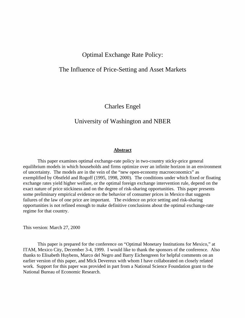
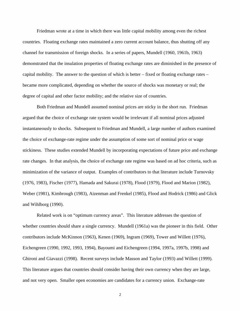
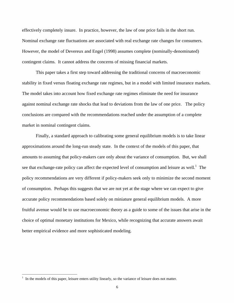
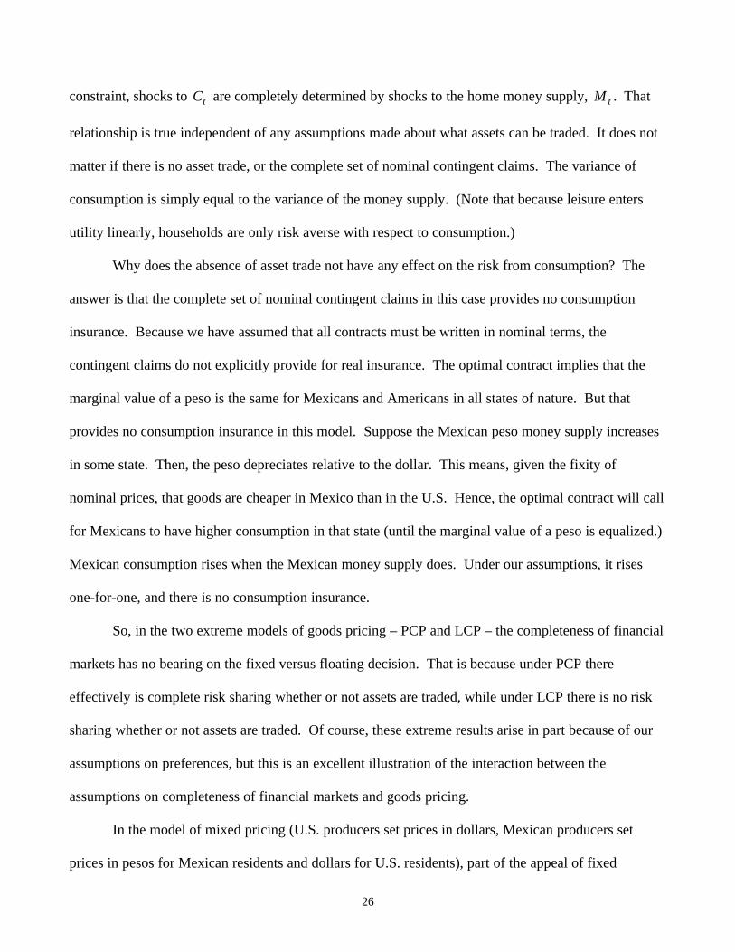
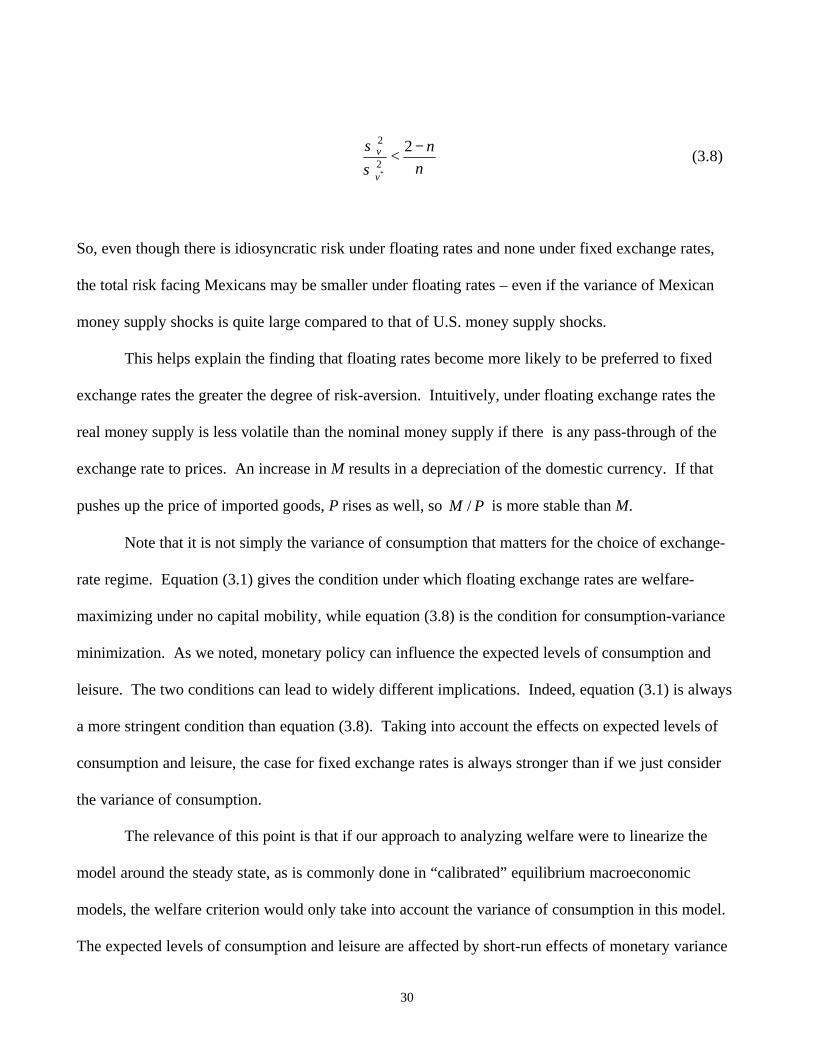
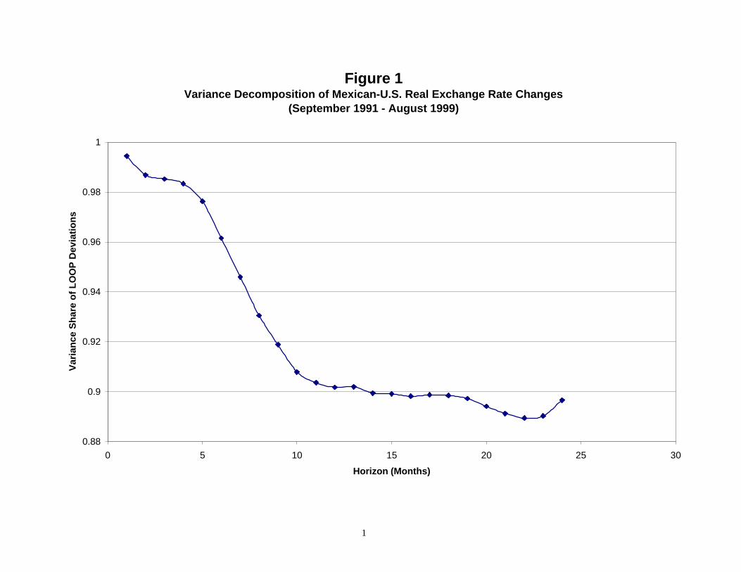
Figure 1 plots jϕ for 24,...2,1=j . Given that there are only eight years of monthly data, one

must treat the estimated longer variances with some skepticism.

10

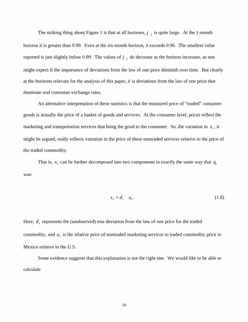
The striking thing about Figure 1 is that at all horizons, jϕ is quite large. At the 1-month

horizon it is greater than 0.99. Even at the six-month horizon, it exceeds 0.96. The smallest value

reported is just slightly below 0.89. The values of jϕ do decrease as the horizon increases, as one

might expect if the importance of deviations from the law of one price diminish over time. But clearly

at the horizons relevant for the analysis of this paper, it is deviations from the law of one price that

dominate real consumer exchange rates.

An alternative interpretation of these statistics is that the measured price of “traded” consumer

goods is actually the price of a basket of goods and services. At the consumer level, prices reflect the

marketing and transportation services that bring the good to the consumer. So, the variation in tx , it

might be argued, really reflects variation in the price of these nontraded services relative to the price of

the traded commodity.

That is, tx can be further decomposed into two components in exactly the same way that tq

was:

ttt udx += . (1.8)

Here, td represents the (unobserved) true deviation from the law of one price for the traded

commodity, and tu is the relative price of nontraded marketing services to traded commodity price in

Mexico relative to the U.S.

Some evidence suggests that this explanation is not the right one. We would like to be able to

calculate

11

)(

)(~

tjt

tjtj qqVar

ddVar

−

−=

+

+ϕ .

Assume the true deviations from the law of one price, td , are uncorrelated with tu and ty . Then,

( ))(

)(

),( 22

tjtjtjt

tjttjtj uuVar

yyVar

yyxxCov−=

−

−−≡ +

+

++ ρθ .

jθ measures the “explained” variance in a regression of tjt xx −+ on tjt yy −+ . jρ is the correlation

coefficient between tjt uu −+ and tjt yy −+ . (The measure of the ty component is derived from tx

and tq : ttt xqy −= .)

This statistic can be used in two ways to get a sense of how plausible the marketing story is.

First, assume 1=ρ , so that the relative price of nontraded marketing services to commodities is

perfectly correlated with the general relative price of nontraded goods. Then,

)(

)(~

tjt

jtjtj qqVar

xxVar

−

−−=

+

+ θϕ .

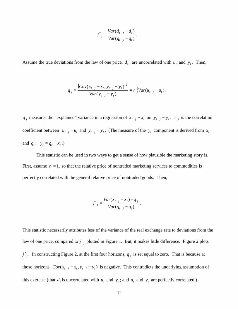
This statistic necessarily attributes less of the variance of the real exchange rate to deviations from the

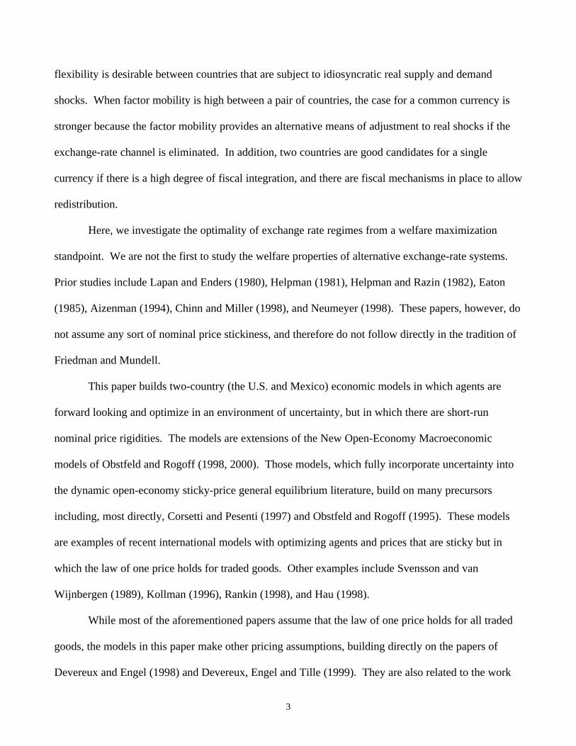
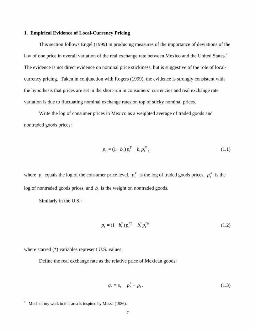
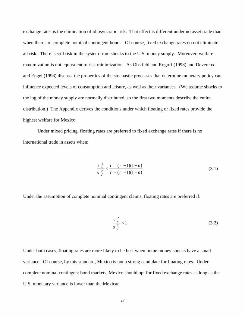
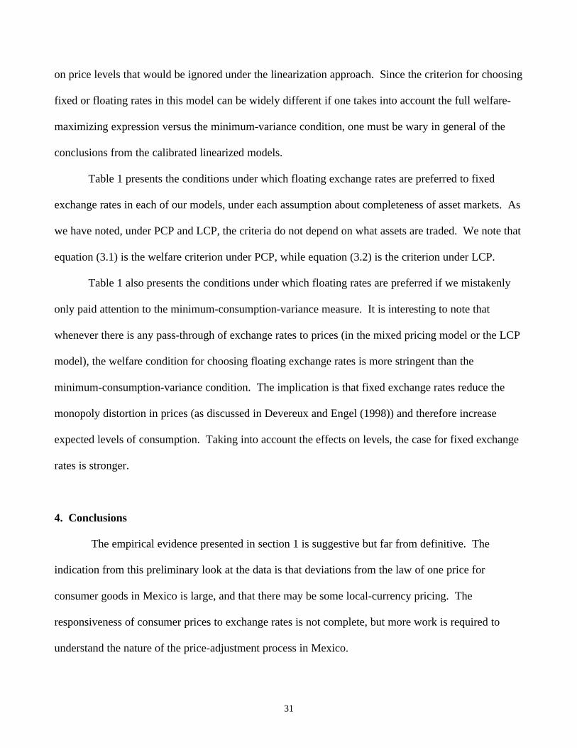
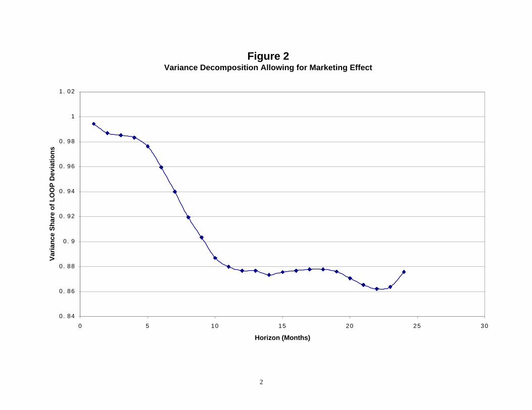
law of one price, compared to jϕ plotted in Figure 1. But, it makes little difference. Figure 2 plots

jϕ~ . In constructing Figure 2, at the first four horizons, jθ is set equal to zero. That is because at

those horizons, ),( tjttjt yyxxCov −− ++ is negative. This contradicts the underlying assumption of

this exercise (that td is uncorrelated with tu and ty ; and tu and ty are perfectly correlated.)

12

The lesson from Figure 2 is that if the relative price of nontraded marketing services behaves

just like the relative price of other nontraded goods, it cannot be a very large component of tx since

),( tjttjt yyxxCov −− ++ is quite small at all horizons.

Perhaps a fairer test of the marketing hypothesis would be to allow the correlation of tu and ty

to be less than perfect. That correlation is not easily identified. But, note more generally

)(

)/()(~2

tjt

jjtjtj qqVar

xxVar

−

−−=

+

+ ρθϕ .

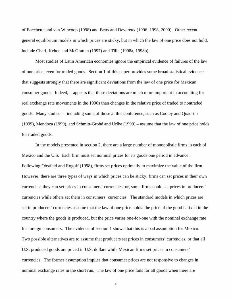
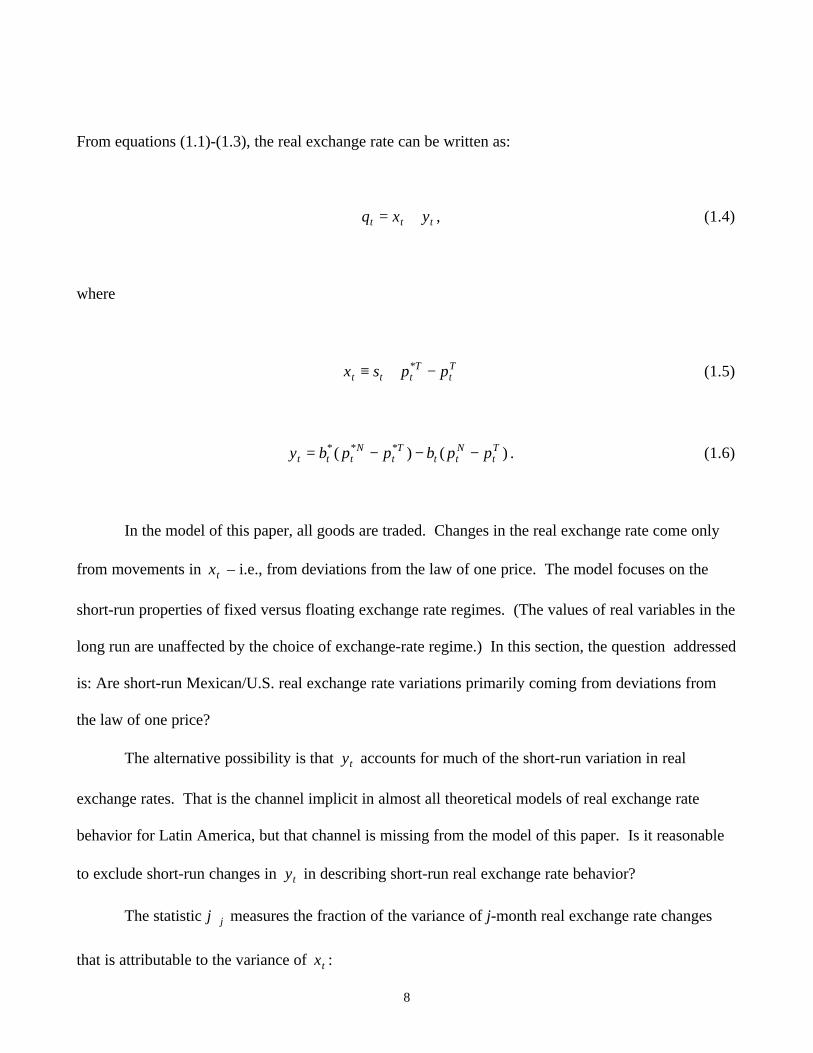
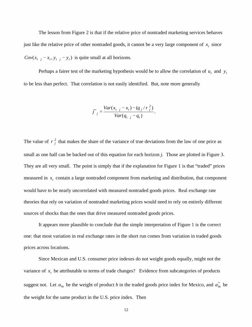
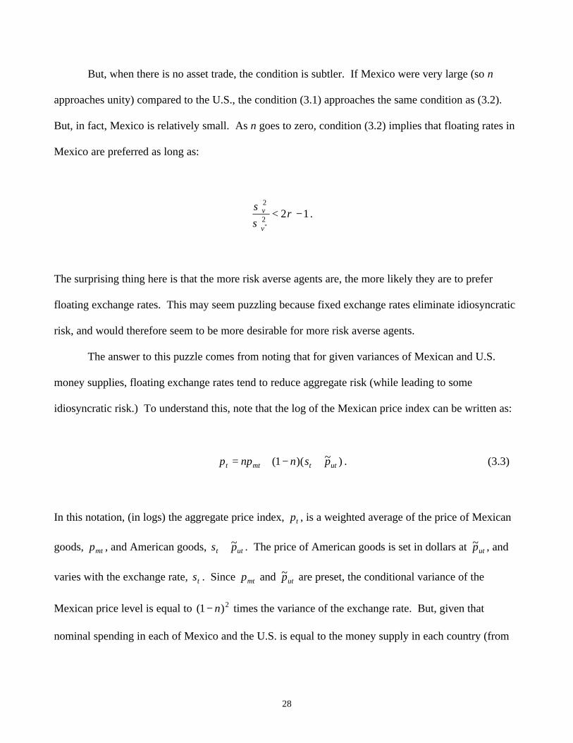
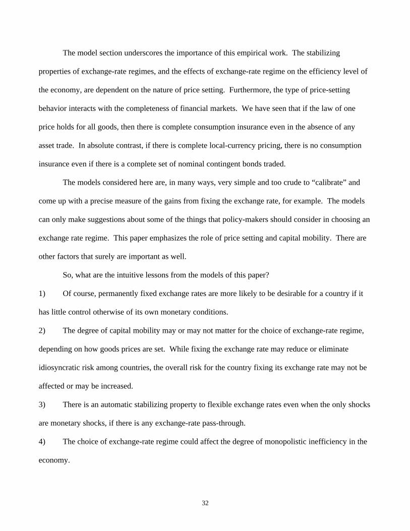
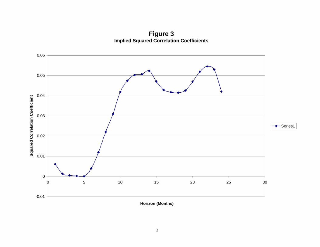
The value of 2jρ that makes the share of the variance of true deviations from the law of one price as

small as one half can be backed out of this equation for each horizon j. Those are plotted in Figure 3.

They are all very small. The point is simply that if the explanation for Figure 1 is that “traded” prices

measured in tx contain a large nontraded component from marketing and distribution, that component

would have to be nearly uncorrelated with measured nontraded goods prices. Real exchange rate

theories that rely on variation of nontraded marketing prices would need to rely on entirely different

sources of shocks than the ones that drive measured nontraded goods prices.

It appears more plausible to conclude that the simple interpretation of Figure 1 is the correct

one: that most variation in real exchange rates in the short run comes from variation in traded goods

prices across locations.

Since Mexican and U.S. consumer price indexes do not weight goods equally, might not the

variance of tx be attributable to terms of trade changes? Evidence from subcategories of products

suggest not. Let hta be the weight of product h in the traded goods price index for Mexico, and *hta be

the weight for the same product in the U.S. price index. Then

13

∑ =+=

k

iiti

hth

Tt papap

1, hi ≠

∑ =+=

k

ii

tih

thT

t papap1

***** , hi ≠

It follows that

ht

htt wvx += ,

where tx is defined as in equation (1.5), and

ht

htt

ht ppsv −+≡ * ,

∑∑ ==−−−≡

k

iht

iti

k

ih

ti

tiht ppappaw

11*** )()( .

If the law of one price holds for all goods, then 0=htv and

∑ =−−≡

k

iht

itii

ht ppaaw

1* ))(( .

When the law of one price holds for all goods, changes in the real exchange rate only occur when the

relative price of individual traded goods change, and those traded goods have different weights in the

U.S. and Mexican price indexes. For example, if food has a higher weight in the Mexican traded

14

consumer price index compared to the U.S., then an increase in the price of food relative to other

traded goods will raise the Mexican traded consumer price index relative to that in the U.S.

If the law of one price holds, the statistic hjϕ̂ , defined by

)(

)(ˆ

tjt

ht

hjth

j xxVar

vvVar

−

−=

+

+ϕ

should be zero at all horizons. Conversely, if the law of one price does not hold, hjϕ̂ should be large

for many goods.

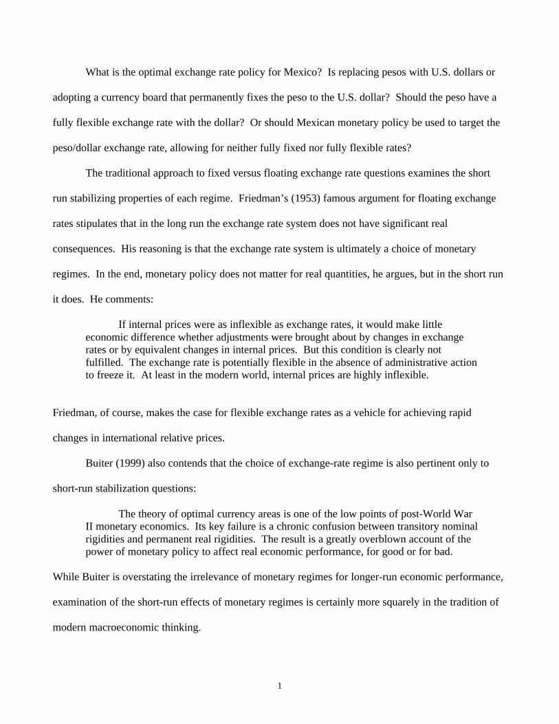
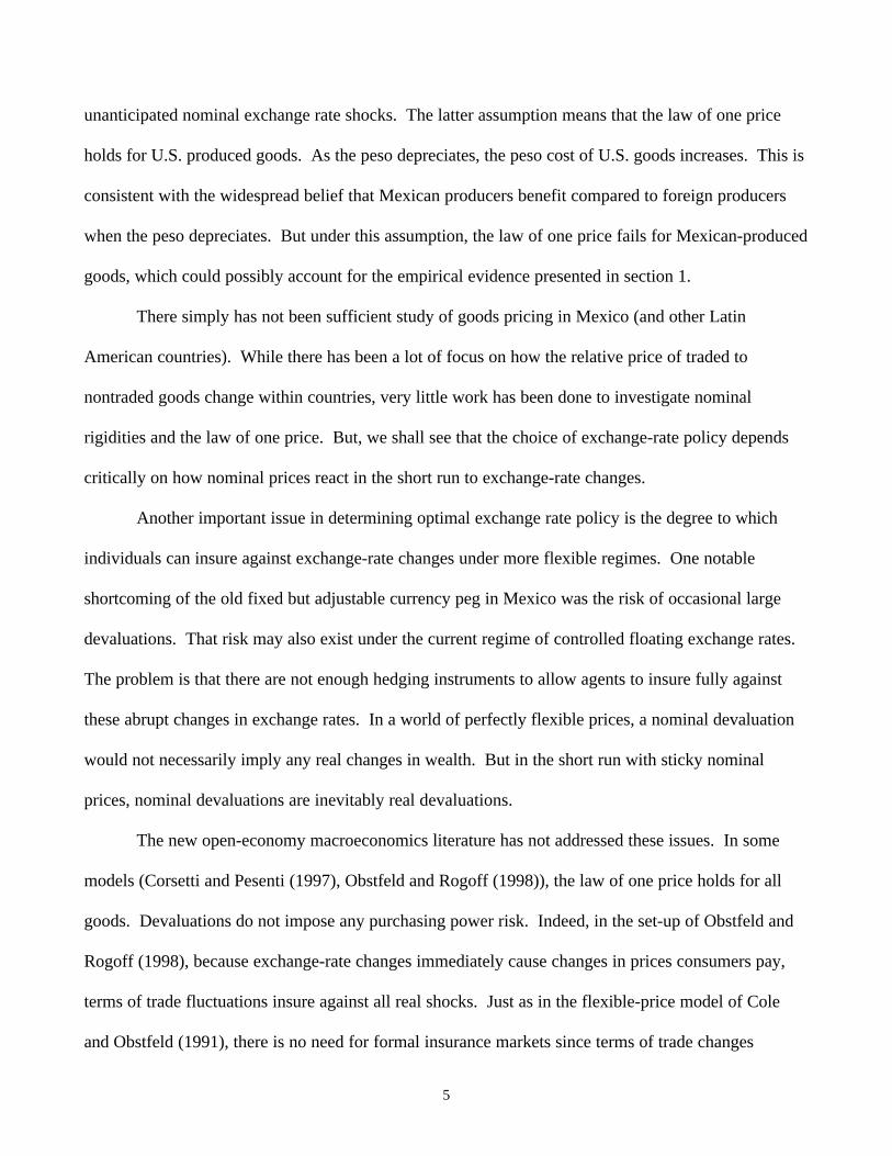
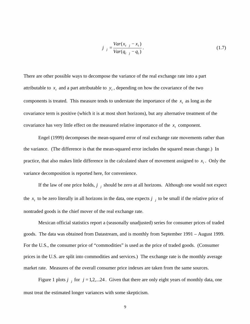
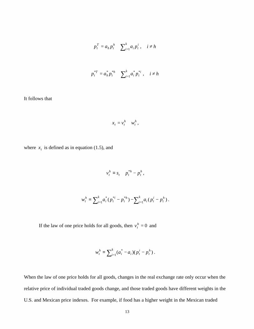
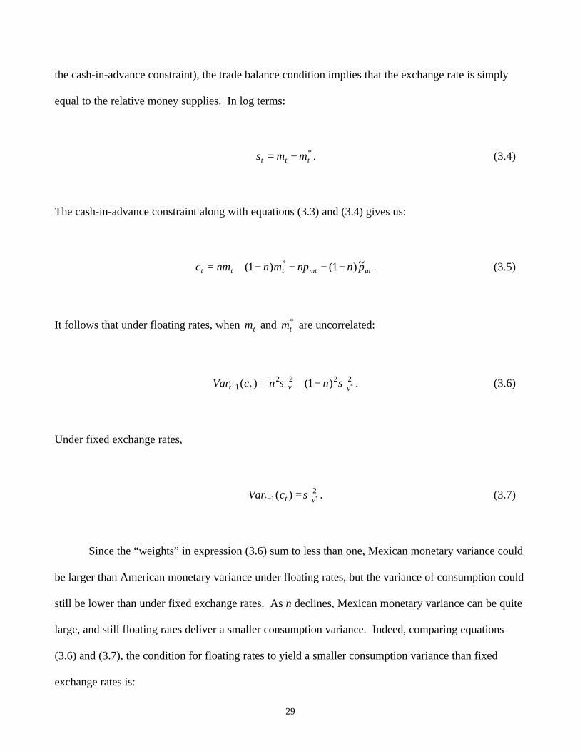
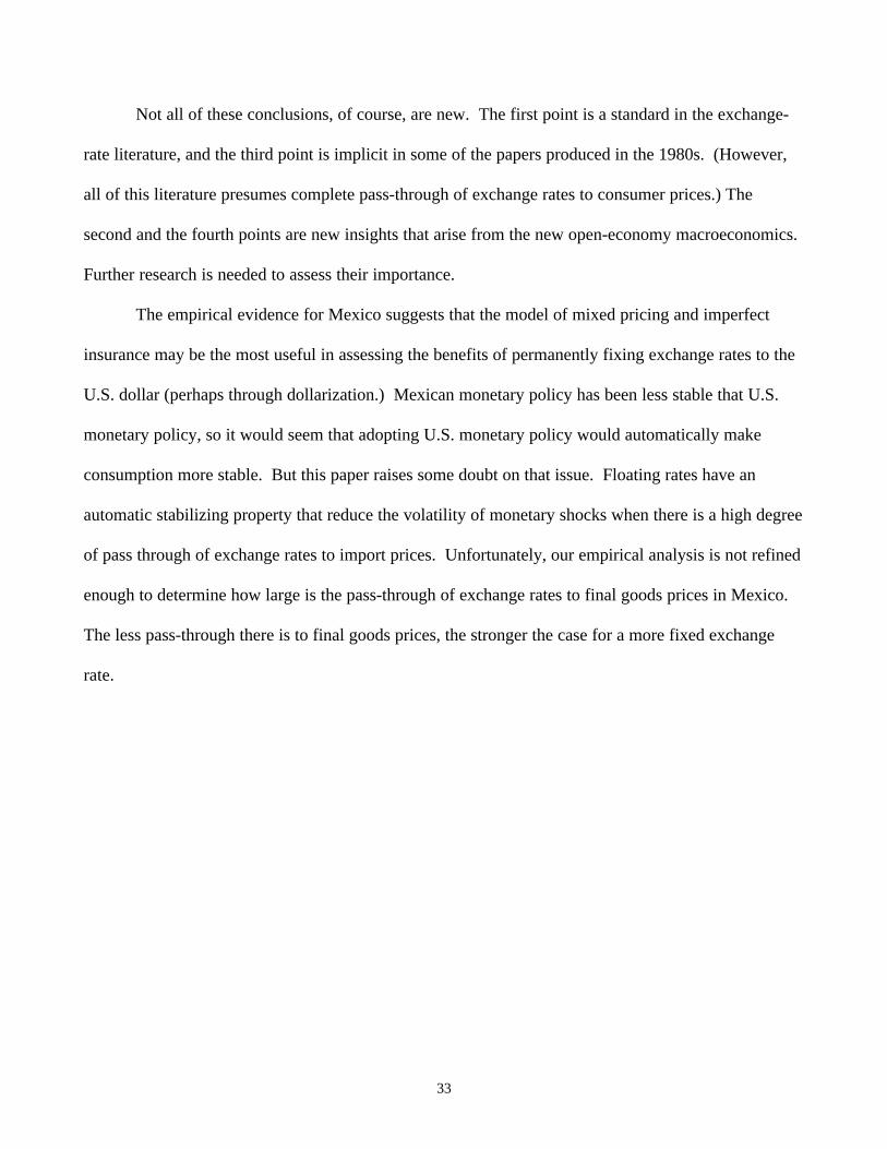
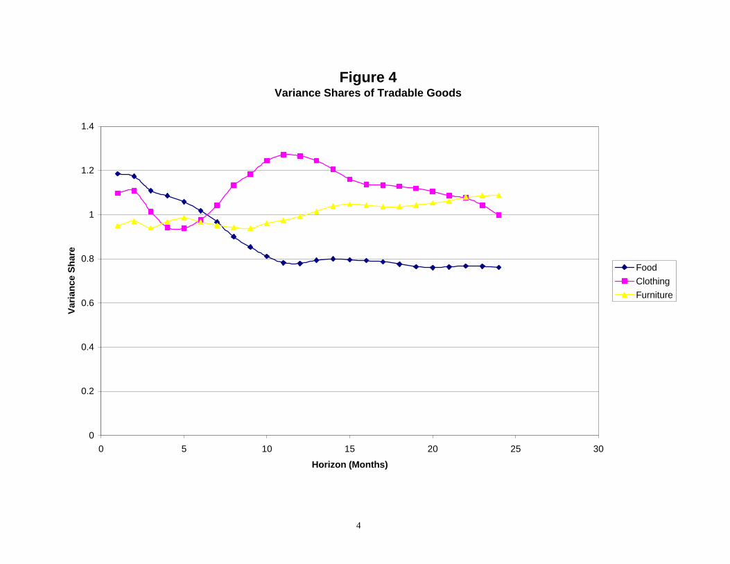
Figure 4 plots hjϕ̂ for 24,...2,1=j . The plots are for three categories of goods that are

primarily traded: food, household furnishings, and apparel. The data sources and dates are the same as

those described above.

The evidence from Figure 4 supports the presumption that movement in tx in the short run

comes from deviations from the law of one price. At all horizons plotted, for all three categories of

goods, hjϕ̂ is large – not at all close to zero.

Of course, it is possible that at some finer level of disaggregation, there are significant changes

in relative traded goods prices within Mexico and the U.S. that are driving movements in hjϕ̂ . At some

level this is tautologically true: goods sold to consumers in Mexico and in U.S. are different goods

because the location the good is sold is part of the characteristic of the good. But the statistics

presented in Figures 1-4 limit the types of models of real exchange rate behavior one might appeal to if

one rejects the interpretation that failures of the law of one price drive the real exchange rate.

15

Finally, if the law of one price fails, is it because of local-currency pricing? The models

considered in this paper assume that for some goods there is local-currency pricing. That is, at least

some producers set nominal prices in consumers’ currencies.

There are two pieces of evidence that appear to support the local-currency-pricing story. First

is Rogers’s (1999) study of consumer prices in Mexico, the U.S. and Canada. In his study, data on

aggregate consumer prices for cities in those three countries is examined. He finds that distance

between cities explains much of the variation in relative price levels. That evidence supports the

notion that the law of one price fails because of transportation costs and other real factors that drive a

wedge between prices in different locations. But, even taking into account distance, relative price

levels vary to a much greater degree for city pairs that lie across national borders than for city pairs

that lie within a country.3 This evidence is consistent with the local-currency pricing effect. Indeed,

the relative sizes of the U.S./Mexico, U.S./Canada, and Canada/Mexico border effects are nearly

identical to the relative sizes of the nominal exchange rate variance for those countries.

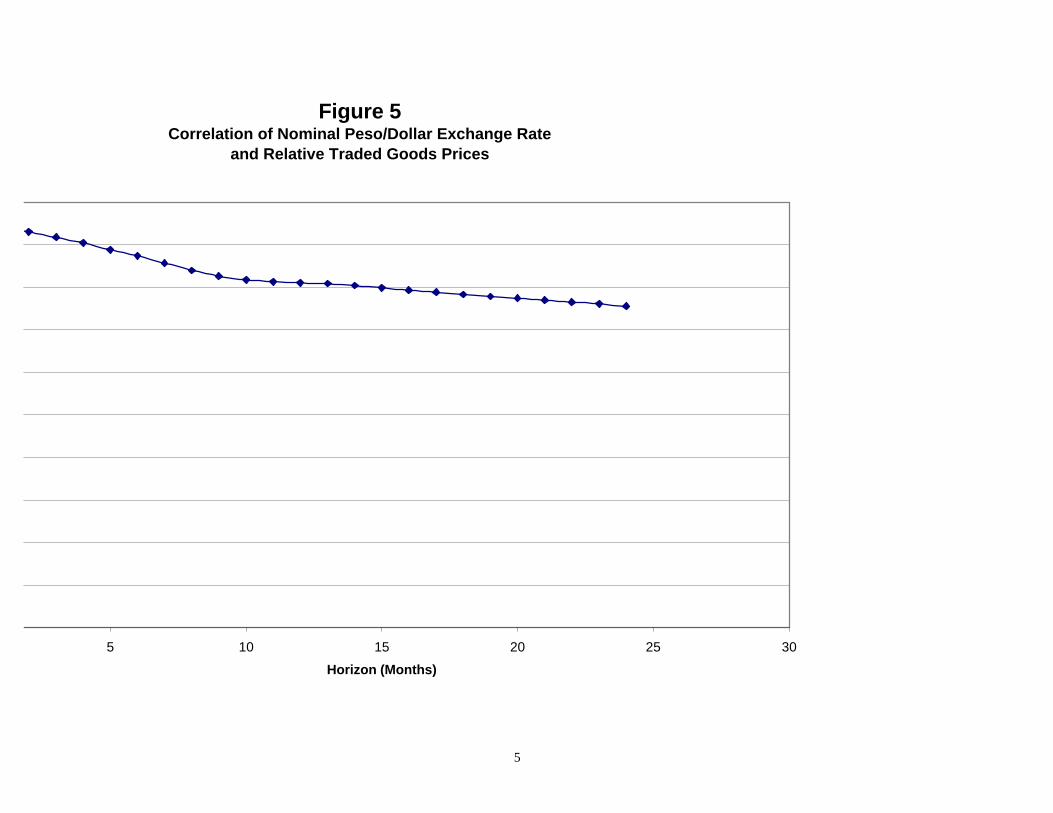
Some simple direct evidence comes from examining the correlation of the nominal exchange

rate with tx . Figure 5 plots values of the correlation of tjt xx −+ with tjt ss −+ . It shows that at

horizons 24,...2,1=j , the correlation is greater than 0.75. At shorter horizons, the correlation exceeds

0.90. So, an approximately accurate description of the data is that Ttp and T

tp* are constant or very

slow moving, while ts varies much more over time.

That does not necessarily imply that nominal prices are sticky, in the sense that they are not

responding to forces of supply and demand. Perhaps it is the case that Ttp and T

tp* are relatively

constant over time because monetary policy does a good job in stabilizing nominal prices. Under this

3 Rogers (1999) thus extends the analysis of Engel and Rogers (1996) to include Mexico, and finds similar results. Notehowever that Rogers (1999) uses only aggregate consumer prices, while Engel and Rogers (1996) use somewhatdisaggregated price indexes.

16

theory, movement in tx really does represent changes in the real forces that segment Mexican and

American markets. But this explanation has a curious implication. Since monetary policy is

stabilizing Ttp and T

tp* , the nominal exchange rate must do all of the adjustment in response to these

changes in market segmentation. In short, it is a theory under which nominal exchange rate changes

are entirely determined by transportation costs! This is an implausible alternative to the simple

conclusion that Ttp and T

tp* are stable because consumer prices adjust more slowly than nominal

exchange rates.

The data is consistent with the local-currency pricing assumption. Perhaps other models can

explain the consumer price data as well, but, inescapably, they would be unusual theories.

2. The Models

In this section, we investigate two-country models. We label the countries Mexico and the

United States. The models of this section assume that all goods produced are final consumer goods.

The goods are produced in monopolistically competitive markets. In each country there are a large

number of goods produced, each of which is an imperfect substitute for all other goods. Producers

must set prices one period in advance.

As is well known from the menu-cost literature, the monopolistic assumption has several

advantages for motivating sticky-price models in which output is demand-determined in the short run.

In the first place, the notion that firms can set prices, in itself, implies some market power for

producers. A producer in competitive markets must take market prices as given and cannot announce a

price in advance. But monopolistic producers are able to set prices for their products, and may not

change those preset prices in response to supply or demand shocks if there are menu costs and the size

17

of the shocks is sufficiently small. Since producers are monopolists, they set prices above marginal

costs. If there is an increase in demand for the product, the producer is willing to increase output to

satisfy demand at preset prices as long as the increase in demand does not push into a region where

marginal costs exceed the price. So, the monopolistic setting offers a rationale for demand-determined

output. This “New Keynesian” approach also offers a rationale for macroeconomic policies that might

stimulate output. Because monopolistic producers choose inefficiently low output levels, policies that

can increase average output might be desirable.

The only source of uncertainty in these models is monetary uncertainty. It is straightforward to

introduce other types of uncertainty – for example, uncertainty arising from productivity shocks or

fiscal shocks. There are three reasons why we restrict attention to monetary shocks. First, the

consensus of the papers of this conference is that the chief reason for Mexico to consider alternative

monetary institutions is dissatisfaction with Mexico’s control of monetary policy in recent years.

Monetary shocks (perhaps arising from the banking sector) seem more significant than real

productivity or spending shocks. Second, a major aim of this paper is to demonstrate how difficult it is

to arrive at definitive conclusions about monetary policy in the absence of good emprical evidence on

how goods prices are set and how agents can insure against foreign exchange rate changes. That point

comes through even in models with only monetary shocks. Third, algebraically the model is

complicated enough with only monetary shocks. Other shocks would make things worse.

Households

Households in Mexico are assumed to maximize expected utility over an infinite horizon. They

get utility from consumption and leisure (or, rather, they get disutility from work.) The households

maximize

18

= ∑

∞

=

−

tss

tstt uEU β , 10 << β

where

sss LCu ηρ

ρ −−

= −1

1

1, 0>ρ .

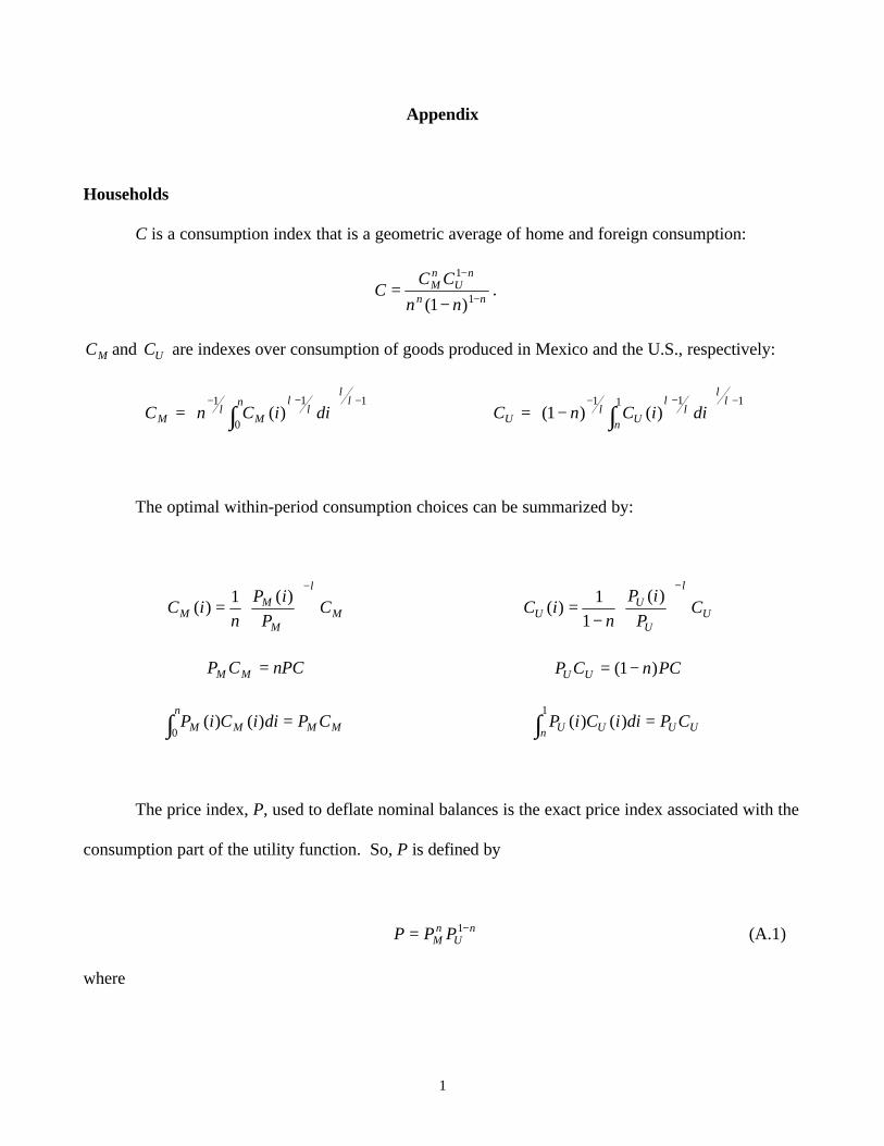
C is a consumption index that is a geometric average of home and foreign consumption, MC and UC .

MC receives a weight of n. There are n identical individuals in Mexico, 10 << n , and n−1 identical

individuals in the U.S., so the weight goods produced in each country receive in the utility function is

equal to the populations proportions. In turn, MC and UC are indexes over continuums of goods

produced in Mexico and the U.S., respectively. (Consumption of the good produced, for example, by

firm i in Mexico is )(iCM .) There is a constant elasticity of substitution between goods produced

within a country, λ , which is greater than 1. Note that following Corsetti and Pesenti’s (1997)

innovation to the Obstfeld and Rogoff (1995) framework, this utility function does not impose that the

elasticity of substitution between goods produced within a country is the same as consumers’ elasticity

of substitution for goods produced in different countries. (See the Appendix for further discussion of

the utility function of consumption.)

L is the labor supply of the representative home agent. U.S. households have preferences

similar to Mexicans’. They have identical preferences over Mexican and American-produced goods.

Labor enters the utility function linearly, but of course Americans get disutility from their own labor.

We impose a cash-in-advance constraint on consumers in both countries. P is the exact price

index for Mexican consumption, so PC equals total nominal spending in Mexico. Mexicans need

peso balances to buy all goods, so we impose:

ttt CPM = ,

19

where M are nominal peso balances. There is an analogous constraint for U.S. households, who must

hold U.S. dollars.

We consider two extreme models of the menu of assets available to households. In the first,

agents can neither borrow nor lend. The budget constraint for the typical Mexican is:

tttttttt TMLWMCP +++=+ −1π .

Agents are endowed with equal ownership in each of their own country’s firms. tπ is the

representative agent’s share of profits from Mexican firms. tT are monetary transfers from the

government. tW is the wage rate.

In the second model, we assume there is a complete set of nominal state-contingent bonds

available to all households in both countries. That is, there is an asset traded for each state of the

world, but payoffs are settled in nominal terms. Agents must then use money payoffs to buy goods at

the nominal prices that are set for them. See Devereux and Engel (1998) for details of this set-up.

Firms

Firms produce output using labor. The production function for a typical Mexican firm is given

by:

tt LY = .

20

The objective of the Mexican firms is to set prices to maximize the expected utility of the firm

owners. Mexican firms are owned by Mexican residents. Firms must set prices for period t before any

information on the stochastic variables – Mexican and American money supply and cost shocks – is

known. No state-contingent pricing is allowed. As Obstfeld and Rogoff (1998) show, this problem

can be expressed as maximizing the expected discounted value of profits using the consumption

discount factor.

We consider the following models for pricing:

1) Producer-currency pricing (PCP). Under this model, the Mexican firm sets prices in peso terms

for sale to both Mexican and American consumers, and American firms set prices in dollars for sale to

both sets of consumers. Of course, the price that Americans actually pay for Mexican goods is a dollar

price, and that price varies instantaneously with changes in the nominal exchange rate. Likewise, the

peso price that Mexicans pay for American goods varies with the exchange rate.

While, in principal, the Mexican firm could set a different peso price for sale to Mexicans and

Americans, given the assumption of identical preferences it is clear it will choose the same ex ante

price. Given the stationarity of the model, firm i in Mexico chooses )(iPMt to maximize:

( )[ ]

+−

−−

−−

− )()())(( *

1

11 iXiXWiP

CP

PCE MtMttMt

tt

ttt ρ

ρβ.

In this expression, )()( inCiX MtMt ≡ represents total sales of the Mexican good to Mexicans, and

)()1()( ** iCniX MtMt −≡ are total sales of the Mexican good to Americans. American firms face an

analogous problem. The optimal pricing rules are derived in the Appendix.

21

2) Local-currency pricing (LCP). In this model, the Mexican firm chooses a peso price for

Mexican consumers and a dollar price for American consumers, ex ante. The prices are set one period

in advance and do not change when the exchange rate changes. Likewise, American firms set a dollar

price for American consumers and a peso price for Mexicans.

Firm i in Mexico chooses )(iPMt (the price Mexicans pay for Mexican goods) and )(* iPMt (the

dollar price that Americans pay for Mexican goods) to maximize:

( )[ ]

+−+

−−

−−

− )()()()()()( ***

1

11 iXiXWiXiPSiXiP

CP

PCE MtMttMtMttMtMt

tt

ttt ρ

ρβ.

In this expression, tS is the peso/dollar exchange rate.

3) Mixed pricing. In this model, it is assumed that Mexican producers set a dollar price for U.S.

consumers and a peso price for Mexican consumers, but U.S. producers set all prices in dollars. So,

Mexican firms are LCP pricers, but U.S. firms are PCP pricers.

While the empirical evidence of section 1 indicates the law of one price does not hold for all

goods, the data is not nearly refined enough to distinguish between pricing assumption (2) and (3).

The mixed pricing assumption might be plausible given the commonly-held observation that

depreciation of the peso helps Mexican producers relative to U.S. producers. Under the mixed pricing

model, the price Mexicans pay for Mexican-produced goods is unaffected by exchange-rate changes

but the peso price of U.S. goods increases when the peso depreciates.

22

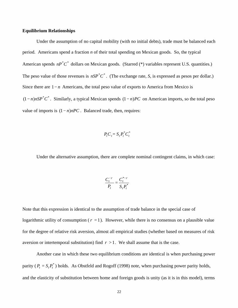
Equilibrium Relationships

Under the assumption of no capital mobility (with no initial debts), trade must be balanced each

period. Americans spend a fraction n of their total spending on Mexican goods. So, the typical

American spends **CnP dollars on Mexican goods. (Starred (*) variables represent U.S. quantities.)

The peso value of those revenues is **CnSP . (The exchange rate, S, is expressed as pesos per dollar.)

Since there are n−1 Americans, the total peso value of exports to America from Mexico is

**)1( CnSPn− . Similarly, a typical Mexican spends PCn)1( − on American imports, so the total peso

value of imports is nPCn)1( − . Balanced trade, then, requires:

**ttttt CPSCP =

Under the alternative assumption, there are complete nominal contingent claims, in which case:

*

*

tt

t

t

t

PS

C

P

C ρρ −−

=

Note that this expression is identical to the assumption of trade balance in the special case of

logarithmic utility of consumption ( 1=ρ ). However, while there is no consensus on a plausible value

for the degree of relative risk aversion, almost all empirical studies (whether based on measures of risk

aversion or intertemporal substitution) find 1>ρ . We shall assume that is the case.

Another case in which these two equilibrium conditions are identical is when purchasing power

parity ( *ttt PSP = ) holds. As Obstfeld and Rogoff (1998) note, when purchasing power parity holds,

and the elasticity of substitution between home and foreign goods is unity (as it is in this model), terms

23

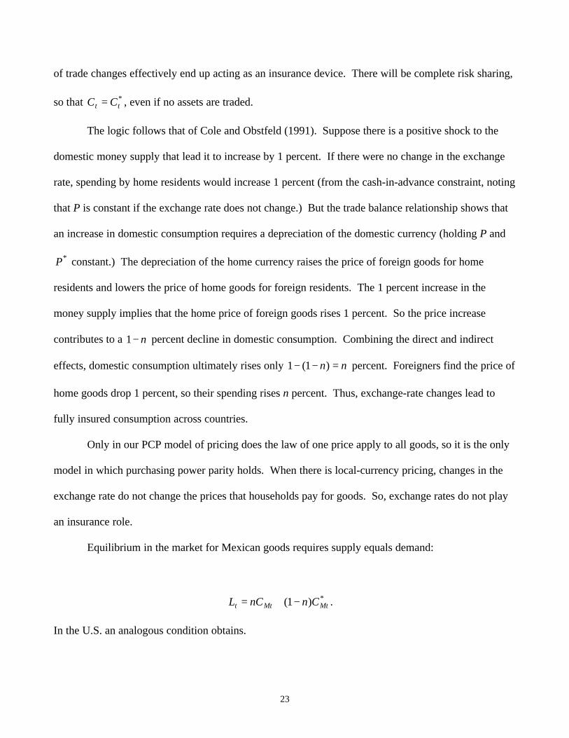
of trade changes effectively end up acting as an insurance device. There will be complete risk sharing,

so that *tt CC = , even if no assets are traded.

The logic follows that of Cole and Obstfeld (1991). Suppose there is a positive shock to the

domestic money supply that lead it to increase by 1 percent. If there were no change in the exchange

rate, spending by home residents would increase 1 percent (from the cash-in-advance constraint, noting

that P is constant if the exchange rate does not change.) But the trade balance relationship shows that

an increase in domestic consumption requires a depreciation of the domestic currency (holding P and

*P constant.) The depreciation of the home currency raises the price of foreign goods for home

residents and lowers the price of home goods for foreign residents. The 1 percent increase in the

money supply implies that the home price of foreign goods rises 1 percent. So the price increase

contributes to a n−1 percent decline in domestic consumption. Combining the direct and indirect

effects, domestic consumption ultimately rises only nn =−− )1(1 percent. Foreigners find the price of

home goods drop 1 percent, so their spending rises n percent. Thus, exchange-rate changes lead to

fully insured consumption across countries.

Only in our PCP model of pricing does the law of one price apply to all goods, so it is the only

model in which purchasing power parity holds. When there is local-currency pricing, changes in the

exchange rate do not change the prices that households pay for goods. So, exchange rates do not play

an insurance role.

Equilibrium in the market for Mexican goods requires supply equals demand:

*)1( MtMtt CnnCL −+= .

In the U.S. an analogous condition obtains.

24

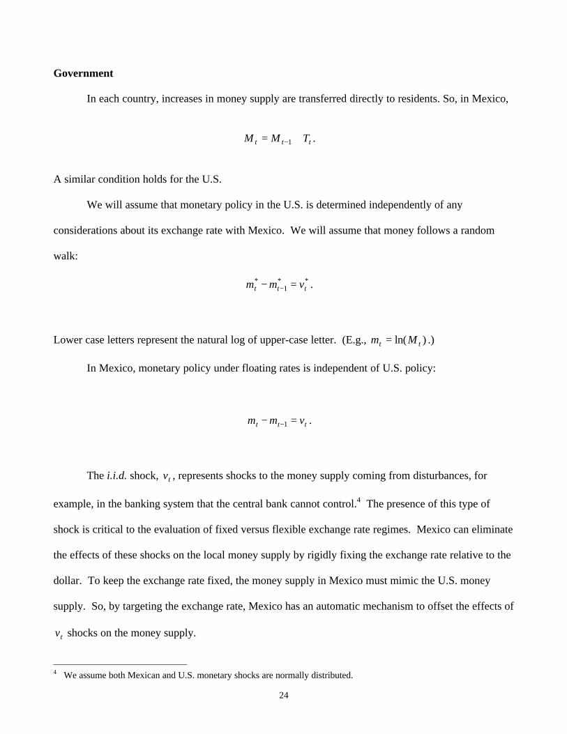
Government

In each country, increases in money supply are transferred directly to residents. So, in Mexico,

ttt TMM += −1 .

A similar condition holds for the U.S.

We will assume that monetary policy in the U.S. is determined independently of any

considerations about its exchange rate with Mexico. We will assume that money follows a random

walk:

**1

*ttt vmm =− − .

Lower case letters represent the natural log of upper-case letter. (E.g., )ln( tt Mm = .)

In Mexico, monetary policy under floating rates is independent of U.S. policy:

ttt vmm =− −1 .

The i.i.d. shock, tv , represents shocks to the money supply coming from disturbances, for

example, in the banking system that the central bank cannot control.4 The presence of this type of

shock is critical to the evaluation of fixed versus flexible exchange rate regimes. Mexico can eliminate

the effects of these shocks on the local money supply by rigidly fixing the exchange rate relative to the

dollar. To keep the exchange rate fixed, the money supply in Mexico must mimic the U.S. money

supply. So, by targeting the exchange rate, Mexico has an automatic mechanism to offset the effects of

tv shocks on the money supply.

4 We assume both Mexican and U.S. monetary shocks are normally distributed.

25

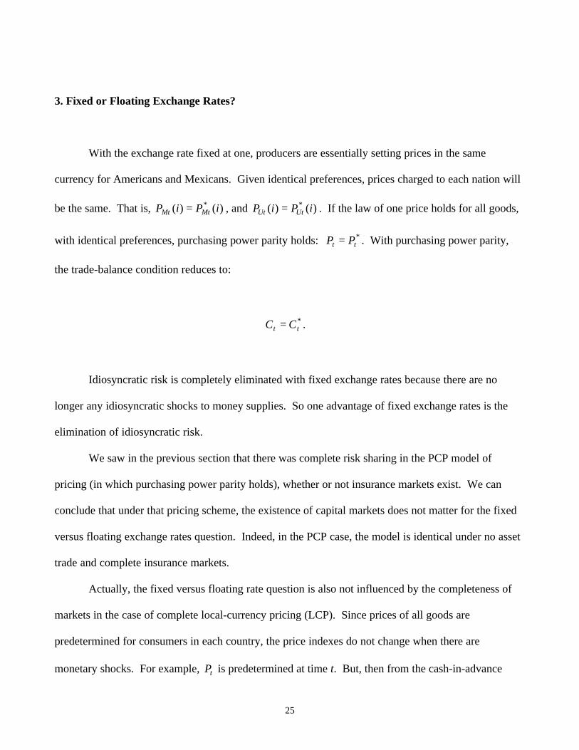
3. Fixed or Floating Exchange Rates?

With the exchange rate fixed at one, producers are essentially setting prices in the same

currency for Americans and Mexicans. Given identical preferences, prices charged to each nation will

be the same. That is, )()( * iPiP MtMt = , and )()( * iPiP UtUt = . If the law of one price holds for all goods,

with identical preferences, purchasing power parity holds: *tt PP = . With purchasing power parity,

the trade-balance condition reduces to:

*tt CC = .

Idiosyncratic risk is completely eliminated with fixed exchange rates because there are no

longer any idiosyncratic shocks to money supplies. So one advantage of fixed exchange rates is the

elimination of idiosyncratic risk.

We saw in the previous section that there was complete risk sharing in the PCP model of

pricing (in which purchasing power parity holds), whether or not insurance markets exist. We can

conclude that under that pricing scheme, the existence of capital markets does not matter for the fixed

versus floating exchange rates question. Indeed, in the PCP case, the model is identical under no asset

trade and complete insurance markets.

Actually, the fixed versus floating rate question is also not influenced by the completeness of

markets in the case of complete local-currency pricing (LCP). Since prices of all goods are

predetermined for consumers in each country, the price indexes do not change when there are

monetary shocks. For example, tP is predetermined at time t. But, then from the cash-in-advance

26

constraint, shocks to tC are completely determined by shocks to the home money supply, tM . That

relationship is true independent of any assumptions made about what assets can be traded. It does not

matter if there is no asset trade, or the complete set of nominal contingent claims. The variance of

consumption is simply equal to the variance of the money supply. (Note that because leisure enters

utility linearly, households are only risk averse with respect to consumption.)

Why does the absence of asset trade not have any effect on the risk from consumption? The

answer is that the complete set of nominal contingent claims in this case provides no consumption

insurance. Because we have assumed that all contracts must be written in nominal terms, the

contingent claims do not explicitly provide for real insurance. The optimal contract implies that the

marginal value of a peso is the same for Mexicans and Americans in all states of nature. But that

provides no consumption insurance in this model. Suppose the Mexican peso money supply increases

in some state. Then, the peso depreciates relative to the dollar. This means, given the fixity of

nominal prices, that goods are cheaper in Mexico than in the U.S. Hence, the optimal contract will call

for Mexicans to have higher consumption in that state (until the marginal value of a peso is equalized.)

Mexican consumption rises when the Mexican money supply does. Under our assumptions, it rises

one-for-one, and there is no consumption insurance.

So, in the two extreme models of goods pricing – PCP and LCP – the completeness of financial

markets has no bearing on the fixed versus floating decision. That is because under PCP there

effectively is complete risk sharing whether or not assets are traded, while under LCP there is no risk

sharing whether or not assets are traded. Of course, these extreme results arise in part because of our

assumptions on preferences, but this is an excellent illustration of the interaction between the

assumptions on completeness of financial markets and goods pricing.

In the model of mixed pricing (U.S. producers set prices in dollars, Mexican producers set

prices in pesos for Mexican residents and dollars for U.S. residents), part of the appeal of fixed

27

exchange rates is the elimination of idiosyncratic risk. That effect is different under no asset trade than

when there are complete nominal contingent bonds. Of course, fixed exchange rates do not eliminate

all risk. There is still risk in the system from shocks to the U.S. money supply. Moreover, welfare

maximization is not equivalent to risk minimization. As Obstfeld and Rogoff (1998) and Devereux

and Engel (1998) discuss, the properties of the stochastic processes that determine monetary policy can

influence expected levels of consumption and leisure, as well as their variances. (We assume shocks to

the log of the money supply are normally distributed, so the first two moments describe the entire

distribution.) The Appendix derives the conditions under which floating or fixed rates provide the

highest welfare for Mexico.

Under mixed pricing, floating rates are preferred to fixed exchange rates if there is no

international trade in assets when:

)1)(1(

)1)(1(2

2

* n

n

v

v

−−−−−+

<ρρρρ

σσ

. (3.1)

Under the assumption of complete nominal contingent claims, floating rates are preferred if:

12

2

*

<v

v

σσ

. (3.2)

Under both cases, floating rates are more likely to be best when home money shocks have a small

variance. Of course, by this standard, Mexico is not a strong candidate for floating rates. Under

complete nominal contingent bond markets, Mexico should opt for fixed exchange rates as long as the

U.S. monetary variance is lower than the Mexican.

28

But, when there is no asset trade, the condition is subtler. If Mexico were very large (so n

approaches unity) compared to the U.S., the condition (3.1) approaches the same condition as (3.2).

But, in fact, Mexico is relatively small. As n goes to zero, condition (3.2) implies that floating rates in

Mexico are preferred as long as:

122

2

*

−< ρσσ

v

v .

The surprising thing here is that the more risk averse agents are, the more likely they are to prefer

floating exchange rates. This may seem puzzling because fixed exchange rates eliminate idiosyncratic

risk, and would therefore seem to be more desirable for more risk averse agents.

The answer to this puzzle comes from noting that for given variances of Mexican and U.S.

money supplies, floating exchange rates tend to reduce aggregate risk (while leading to some

idiosyncratic risk.) To understand this, note that the log of the Mexican price index can be written as:

)~)(1( uttmtt psnnpp +−+= . (3.3)

In this notation, (in logs) the aggregate price index, tp , is a weighted average of the price of Mexican

goods, mtp , and American goods, utt ps ~+ . The price of American goods is set in dollars at utp~ , and

varies with the exchange rate, ts . Since mtp and utp~ are preset, the conditional variance of the

Mexican price level is equal to 2)1( n− times the variance of the exchange rate. But, given that

nominal spending in each of Mexico and the U.S. is equal to the money supply in each country (from

29

the cash-in-advance constraint), the trade balance condition implies that the exchange rate is simply

equal to the relative money supplies. In log terms:

*ttt mms −= . (3.4)

The cash-in-advance constraint along with equations (3.3) and (3.4) gives us:

utmtttt pnnpmnnmc ~)1()1( * −−−−+= . (3.5)

It follows that under floating rates, when tm and *tm are uncorrelated:

22221 *)1()( vvtt nncVar σσ −+=− . (3.6)

Under fixed exchange rates,

21 *)( vtt cVar σ=− . (3.7)

Since the “weights” in expression (3.6) sum to less than one, Mexican monetary variance could

be larger than American monetary variance under floating rates, but the variance of consumption could

still be lower than under fixed exchange rates. As n declines, Mexican monetary variance can be quite

large, and still floating rates deliver a smaller consumption variance. Indeed, comparing equations

(3.6) and (3.7), the condition for floating rates to yield a smaller consumption variance than fixed

exchange rates is:

30

n

n

v

v −<

22

2

*σσ

(3.8)

So, even though there is idiosyncratic risk under floating rates and none under fixed exchange rates,

the total risk facing Mexicans may be smaller under floating rates – even if the variance of Mexican

money supply shocks is quite large compared to that of U.S. money supply shocks.

This helps explain the finding that floating rates become more likely to be preferred to fixed

exchange rates the greater the degree of risk-aversion. Intuitively, under floating exchange rates the

real money supply is less volatile than the nominal money supply if there is any pass-through of the

exchange rate to prices. An increase in M results in a depreciation of the domestic currency. If that

pushes up the price of imported goods, P rises as well, so PM / is more stable than M.

Note that it is not simply the variance of consumption that matters for the choice of exchange-

rate regime. Equation (3.1) gives the condition under which floating exchange rates are welfare-

maximizing under no capital mobility, while equation (3.8) is the condition for consumption-variance

minimization. As we noted, monetary policy can influence the expected levels of consumption and

leisure. The two conditions can lead to widely different implications. Indeed, equation (3.1) is always

a more stringent condition than equation (3.8). Taking into account the effects on expected levels of

consumption and leisure, the case for fixed exchange rates is always stronger than if we just consider

the variance of consumption.

The relevance of this point is that if our approach to analyzing welfare were to linearize the

model around the steady state, as is commonly done in “calibrated” equilibrium macroeconomic

models, the welfare criterion would only take into account the variance of consumption in this model.

The expected levels of consumption and leisure are affected by short-run effects of monetary variance

31

on price levels that would be ignored under the linearization approach. Since the criterion for choosing

fixed or floating rates in this model can be widely different if one takes into account the full welfare-

maximizing expression versus the minimum-variance condition, one must be wary in general of the

conclusions from the calibrated linearized models.

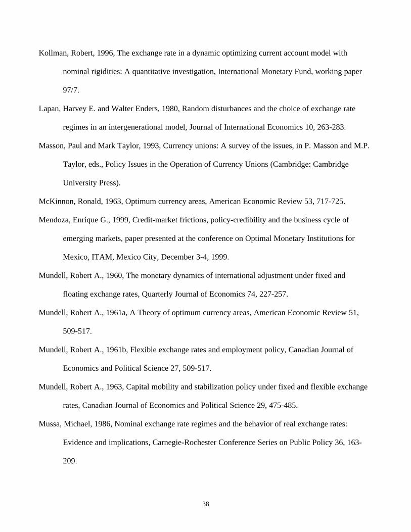
Table 1 presents the conditions under which floating exchange rates are preferred to fixed

exchange rates in each of our models, under each assumption about completeness of asset markets. As

we have noted, under PCP and LCP, the criteria do not depend on what assets are traded. We note that

equation (3.1) is the welfare criterion under PCP, while equation (3.2) is the criterion under LCP.

Table 1 also presents the conditions under which floating rates are preferred if we mistakenly

only paid attention to the minimum-consumption-variance measure. It is interesting to note that

whenever there is any pass-through of exchange rates to prices (in the mixed pricing model or the LCP

model), the welfare condition for choosing floating exchange rates is more stringent than the

minimum-consumption-variance condition. The implication is that fixed exchange rates reduce the

monopoly distortion in prices (as discussed in Devereux and Engel (1998)) and therefore increase

expected levels of consumption. Taking into account the effects on levels, the case for fixed exchange

rates is stronger.

4. Conclusions

The empirical evidence presented in section 1 is suggestive but far from definitive. The

indication from this preliminary look at the data is that deviations from the law of one price for

consumer goods in Mexico is large, and that there may be some local-currency pricing. The

responsiveness of consumer prices to exchange rates is not complete, but more work is required to

understand the nature of the price-adjustment process in Mexico.

32

The model section underscores the importance of this empirical work. The stabilizing

properties of exchange-rate regimes, and the effects of exchange-rate regime on the efficiency level of

the economy, are dependent on the nature of price setting. Furthermore, the type of price-setting

behavior interacts with the completeness of financial markets. We have seen that if the law of one

price holds for all goods, then there is complete consumption insurance even in the absence of any

asset trade. In absolute contrast, if there is complete local-currency pricing, there is no consumption

insurance even if there is a complete set of nominal contingent bonds traded.

The models considered here are, in many ways, very simple and too crude to “calibrate” and

come up with a precise measure of the gains from fixing the exchange rate, for example. The models

can only make suggestions about some of the things that policy-makers should consider in choosing an

exchange rate regime. This paper emphasizes the role of price setting and capital mobility. There are

other factors that surely are important as well.

So, what are the intuitive lessons from the models of this paper?

1) Of course, permanently fixed exchange rates are more likely to be desirable for a country if it

has little control otherwise of its own monetary conditions.

2) The degree of capital mobility may or may not matter for the choice of exchange-rate regime,

depending on how goods prices are set. While fixing the exchange rate may reduce or eliminate

idiosyncratic risk among countries, the overall risk for the country fixing its exchange rate may not be

affected or may be increased.

3) There is an automatic stabilizing property to flexible exchange rates even when the only shocks

are monetary shocks, if there is any exchange-rate pass-through.

4) The choice of exchange-rate regime could affect the degree of monopolistic inefficiency in the

economy.

33

Not all of these conclusions, of course, are new. The first point is a standard in the exchange-

rate literature, and the third point is implicit in some of the papers produced in the 1980s. (However,

all of this literature presumes complete pass-through of exchange rates to consumer prices.) The

second and the fourth points are new insights that arise from the new open-economy macroeconomics.

Further research is needed to assess their importance.

The empirical evidence for Mexico suggests that the model of mixed pricing and imperfect

insurance may be the most useful in assessing the benefits of permanently fixing exchange rates to the

U.S. dollar (perhaps through dollarization.) Mexican monetary policy has been less stable that U.S.

monetary policy, so it would seem that adopting U.S. monetary policy would automatically make

consumption more stable. But this paper raises some doubt on that issue. Floating rates have an

automatic stabilizing property that reduce the volatility of monetary shocks when there is a high degree

of pass through of exchange rates to import prices. Unfortunately, our empirical analysis is not refined

enough to determine how large is the pass-through of exchange rates to final goods prices in Mexico.

The less pass-through there is to final goods prices, the stronger the case for a more fixed exchange

rate.

34

References

Aizenman, Joshua, 1994, Monetary and real shocks, productive capacity and exchange-rate regimes,

Economica, 407-434.

Aizenman, Joshua, and Jacob A. Frenkel, 1985, Optimal wage indexation, foreign exchange

intervention and monetary policy, American Economic Review 75, 402-423.

Bacchetta, Philippe, and Eric van Wincoop, 1998, Does exchange rate stability increase trade and

capital flows, Federal Reserve Bank of New York, working paper no. 9818.

Bayoumi, Tamim, and Barry Eichengreen, 1994, One Money or Many? Analyzing the Prospects for

Monetary Unification in Various Parts of the World, Princeton Studies in International Finance,

76.

Bayoumi, Tamim, and Barry Eichengreen, 1997a, Optimum currency area and exchange rate volatility:

theory and evidence compared, in B.J. Cohen, ed., International Trade and Finance: New

Frontiers in Research, (Cambridge: Cambridge University Press).

Bayoumi, Tamim, and Barry Eichengreen, 1997b, Ever closer to heaven? An optimum currency area

index for European countries, European Economic Review 41, 761-770.

Bayoumi, Tamim, and Barry Eichengreen, 1998, Exchange rate volatility and intervention:

implications of the theory of optimum currency areas, Journal of International Economics 45,

191-209.

Betts, Caroline and Michael B. Devereux, 1996, The exchange rate in a model of pricing-to-market,

European Economic Review 40, 1007-1021.

Betts, Caroline and Michael B. Devereux, 1998, The international effects of monetary and fiscal policy

in a two-country model, University of Southern California, working paper.

35

Betts, Caroline, and Michael B. Devereux, 2000, Exchange rate dynamics in a model of pricing-to-

market, Journal of International Economics 50, 215-244.

Buiter, Willem, 1999, The EMU and the NAMU: What is the case for North American Monetary

Union?, Canadian Journal of Economics, forthcoming.

Chari, V.V.; Patrick J. Kehoe; and, Ellen McGrattan, 1997, Monetary policy and the real exchange rate

in sticky price models of the international business cycle, National Bureau of Economic

Research, working paper no. 5876.

Chinn, Daniel M., and Preston J. Miller, 1998, Fixed vs. floating rates: A dynamic general equilibrium

analysis, European Economic Review 42, 1221-1249.

Cole, Harold L., and Maurice Obstfeld, 1991, Commodity trade and international risk sharing: How

much do financial markets matter?, Journal of Monetary Economics 23, 377-400.

Cooley, Thomas F. and Vincent Quadrini, 1999, The costs of losing monetary independence: The case

of Mexico, paper presented at the conference on Optimal Monetary Institutions for Mexico,

ITAM, Mexico City, December 3-4, 1999.

Corsetti, Giancarlo, and Paolo Pesenti, 1997, Welfare and macroeconomic interdependence, National

Bureau of Economic Research, working paper no. 6307.

Devereux, Michael B., and Charles Engel, 1998, Fixed vs. floating exchange rates: How price setting

affects the optimal choice of exchange-rate regime, National Bureau of Economic Research,

working paper no. 6867.

Devereux, Michael B.; Engel, Charles; and, Cedric Tille, 1999, Exchange rate pass-through and the

welfare effects of the euro, National Bureau of Economics, working paper no. 7382.

Eaton, Jonathan, 1985, Optimal and time consistent exchange rate management in an overlapping

generations economy, Journal of International Money and Finance 4, 83-100.

36

Eichengreen, Barry, 1990, One money for Europe? Lessons from the U.S. currency union, Economic

Policy 10, 117-187.

Eichengreen, Barry, 1992, Is Europe an optimum currency area?, in H. Grubel and S. Border, eds., The

European Community after 1992: Perspectives from the Outside (Basingstoke, England:

Macmillan).

Eichengreen, Barry, 1993, European monetary unification, Journal of Economic Literature 31, 1321-

1357.

Eichengreen, Barry, 1994, Fiscal policy and EMU, in B. Eichengreen and J. Frieden, eds., The Political

Economy of European Monetary Unification (Boulder, Co.: Westview Press).

Engel, Charles, 1999, Accounting for U.S. real exchange rate changes, Journal of Political Economy

107, 507-538.

Engel, Charles, 2000, Local-currency pricing and the choice of exchange-rate regime, European

Economic Review, forthcoming.

Engel, Charles, and John H. Rogers, 1996, How wide is the border?, American Economic Review 86,

1112-1125.

Fischer, Stanley, 1977, Stability and exchange rate systems in a monetarist model of the balance of

payments, in Robert Z. Aliber, ed., The Political Economy of Monetary Reform (Montclair, NJ:

Allanheld, Oemun).

Flood, Robert P., 1979, Capital mobility and the choice of exchange rate regime, International

Economic Review 2, 405-416.

Flood, Robert P., and Robert J. Hodrick, 1986, Real aspects of exchange rate regime choice with

collapsing fixed rates, Journal of International Economics 21, 215-232.

Flood, Robert P. and Nancy P. Marion, 1982, The transmission of disturbances under alternative

exchange-rate regimes with optimal indexing, Quarterly Journal of Economics 96, 43-66.

37

Frankel, Jeffrey, 1999, No single currency regime is right for all countries or at all times, National

Bureau of Economic Research, working paper no. 7338.

Friedman, Milton, 1953, The case for flexible exchange rates, in Essays in Positive Economics

(Chicago: University of Chicago Press), 157-203.

Ghironi, Fabio and Francesco Giavazzi, 1998, Currency areas, international monetary regimes, and the

employment-inflation tradeoff, Journal of International Economics 45, 259-296.

Glick, Reuven, and Clas Wihlborg, 1990, Real exchange rate effects of monetary shocks under fixed

and flexible exchange rates, Journal of International Economics 28, 267-290.

Hamada, Koichi, and Makoto Sakurai, 1978, International transmission of stagflation under fixed and

flexible exchange rates, Journal of Political Economy 86, 877-895.

Hau, Harald, 1998, Exchange rate determination: The role of factor prices and market segmentation,

Journal of International Economics, forthcoming.

Helpman, Elhanan, 1981, An exploration in the theory of exchange-rate regimes, Journal of Political

Economy 10, 263-283.

Helpman, Elhanan, and Assaf Razin, 1982, A comparison of exchange rate regimes in the presence of

imperfect capital markets, International Economic Review 23, 365-388.

Ingram, James, 1969, The currency area problem, in R.A. Mundell and A.K. Swoboda, eds., Monetary

Problems of the International Economy (Chicago: University of Chicago Press).

Kenen, Peter, 1969, The theory of optimal currency areas: an eclectic view, in R.A. Mundell and A.K.

Swoboda, eds., Monetary Problems of the International Economy (Chicago: University of

Chicago Press).

Kimbrough, Kent, 1983, The information content of the exchange rate and the stability of real output

under alternative exchange-rate regimes, Journal of International Money and Finance 2, 27-38.

38

Kollman, Robert, 1996, The exchange rate in a dynamic optimizing current account model with

nominal rigidities: A quantitative investigation, International Monetary Fund, working paper

97/7.

Lapan, Harvey E. and Walter Enders, 1980, Random disturbances and the choice of exchange rate

regimes in an intergenerational model, Journal of International Economics 10, 263-283.

Masson, Paul and Mark Taylor, 1993, Currency unions: A survey of the issues, in P. Masson and M.P.

Taylor, eds., Policy Issues in the Operation of Currency Unions (Cambridge: Cambridge

University Press).

McKinnon, Ronald, 1963, Optimum currency areas, American Economic Review 53, 717-725.

Mendoza, Enrique G., 1999, Credit-market frictions, policy-credibility and the business cycle of

emerging markets, paper presented at the conference on Optimal Monetary Institutions for

Mexico, ITAM, Mexico City, December 3-4, 1999.

Mundell, Robert A., 1960, The monetary dynamics of international adjustment under fixed and

floating exchange rates, Quarterly Journal of Economics 74, 227-257.

Mundell, Robert A., 1961a, A Theory of optimum currency areas, American Economic Review 51,

509-517.

Mundell, Robert A., 1961b, Flexible exchange rates and employment policy, Canadian Journal of

Economics and Political Science 27, 509-517.

Mundell, Robert A., 1963, Capital mobility and stabilization policy under fixed and flexible exchange

rates, Canadian Journal of Economics and Political Science 29, 475-485.

Mussa, Michael, 1986, Nominal exchange rate regimes and the behavior of real exchange rates:

Evidence and implications, Carnegie-Rochester Conference Series on Public Policy 36, 163-

209.

39

Neumeyer, Pablo A., 1998, Currencies and the allocation of risk: The welfare effects of a monetary

union, American Economic Review 88, 246-259.

Obstfeld, Maurice and Kenneth Rogoff, 1995, Exchange rate dynamics redux, Journal of Political

Economy 103, 624-660.

Obstfeld, Maurice and Kenneth Rogoff, 1996, Foundations of International Macroeconomics

(Cambridge: MIT Press).

Obstfeld, Maurice and Kenneth Rogoff, 1998, Risk and exchange rates, National Bureau of Economic

Research, working paper no. 6694.

Obstfeld, Maurice and Kenneth Rogoff, 2000, New directions for stochastic open economy models,

Journal of International Economic 50, 117-153..

Rankin, Neil, 1998, Nominal rigidity and monetary uncertainty in a small open economy, Journal of

Economic Dynamics and Control 22, 679-702.

Rogers, John H., 1999, How wide is the Rio Grande?, Board of Governors of the Federal Reserve

System, notes.

Schmitt-Grohé, Stephanie and Martin Uríbe, 1999, Stabilization policy and the costs of dollarization,

paper presented at the conference on Optimal Monetary Institutions for Mexico, ITAM, Mexico

City, December 3-4, 1999.

Svensson, Lars E.O., and Sweder van Wijnbergen, 1989, Excess capacity, monopolistic competition,

and international transmission of monetary disturbances, Economic Journal 99, 785-805.

Tille, Cédric, 1998a, The international and domestic welfare effects of monetary shocks under pricing-

to-market, Federal Reserve Bank of New York, working paper.

Tille, Cédric, 1998b, The welfare effects of monetary shocks under pricing-to-market: A general

framework, Federal Reserve Bank of New York, working paper.

40

Tower, Edward and Thomas Willett, 1976, The Theory of Optimum Currency Areas and Exchange

Rate Flexibility, Princeton Special Papers in International Finance, 11.

Turnovsky, Stephen, 1976, The relative stability of alternative exchange rate systems in the presence

of random disturbances, Journal of Money, Credit and Banking 8, 29-50.

Turnovsky, Stephen, 1983, Wage indexation and exchange market intervention in a small open

economy, Canadian Journal of Economics 16, 574-592.

Weber, Warren, 1981, Output variability under monetary policy and exchange-rate rules, Journal of

Political Economy 89, 733-75.

Willett, Thomas, 1999, The OCA approach to exchange rate regimes: A perspective on recent

developments, Claremont Graduate University, working paper.

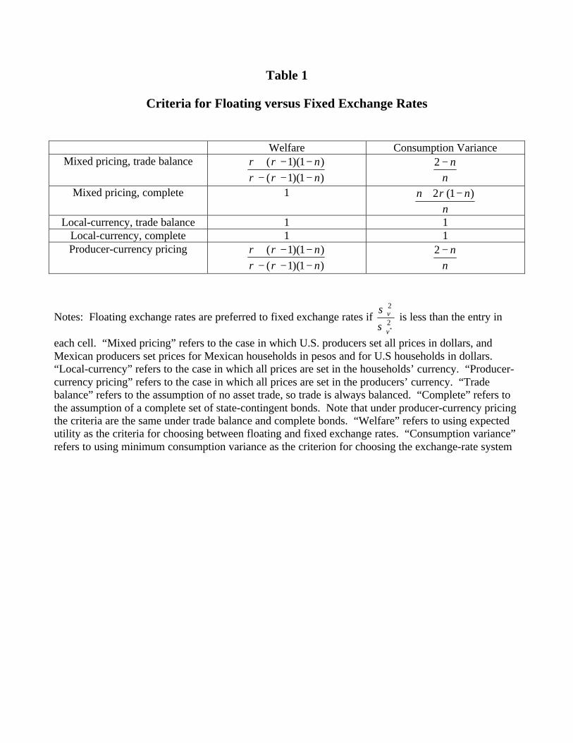
Table 1

Criteria for Floating versus Fixed Exchange Rates

Welfare Consumption VarianceMixed pricing, trade balance

)1)(1(

)1)(1(

n

n

−−−−−+

ρρρρ

n

n−2

Mixed pricing, complete 1

n

nn )1(2 −+ ρ

Local-currency, trade balance 1 1Local-currency, complete 1 1Producer-currency pricing

)1)(1(

)1)(1(

n

n

−−−−−+

ρρρρ

n

n−2

Notes: Floating exchange rates are preferred to fixed exchange rates if 2

2

*v

v

σσ

is less than the entry in

each cell. “Mixed pricing” refers to the case in which U.S. producers set all prices in dollars, andMexican producers set prices for Mexican households in pesos and for U.S households in dollars.“Local-currency” refers to the case in which all prices are set in the households’ currency. “Producer-currency pricing” refers to the case in which all prices are set in the producers’ currency. “Tradebalance” refers to the assumption of no asset trade, so trade is always balanced. “Complete” refers tothe assumption of a complete set of state-contingent bonds. Note that under producer-currency pricingthe criteria are the same under trade balance and complete bonds. “Welfare” refers to using expectedutility as the criteria for choosing between floating and fixed exchange rates. “Consumption variance”refers to using minimum consumption variance as the criterion for choosing the exchange-rate system

1

Figure 1Variance Decomposition of Mexican-U.S. Real Exchange Rate Changes

(September 1991 - August 1999)

0.88

0.9

0.92

0.94

0.96

0.98

1

0 5 10 15 20 25 30

Horizon (Months)

Var

ian

ce S

har

e o

f L

OO

P D

evia

tio

ns

2

Figure 2Variance Decomposition Allowing for Marketing Effect

0. 84

0. 86

0. 88

0. 9

0 . 92

0. 94

0. 96

0. 98

1

1. 02

0 5 10 15 20 25 30

Horizon (Months)

Var

ian

ce S

har

e o

f L

OO

P D

evia

tio

ns

3

Figure 3Implied Squared Correlation Coefficients

-0.01

0

0.01

0.02

0.03

0.04

0.05

0.06

0 5 10 15 20 25 30

Horizon (Months)

Sq

uar

ed C

orr

elat

ion

Co

effi

cien

t

Series1

4

Figure 4Variance Shares of Tradable Goods

0

0.2

0.4

0.6

0.8

1

1.2

1.4

0 5 10 15 20 25 30

Horizon (Months)

Var

ian

ce S

har

e

Food

Clothing

Furniture

5

Figure 5Correlation of Nominal Peso/Dollar Exchange Rate

and Relative Traded Goods Prices

5 10 15 20 25 30

Horizon (Months)

1

Appendix

Households

C is a consumption index that is a geometric average of home and foreign consumption:

nn

nU

nM

nn

CCC −

−

−=

1

1

)1(.

MC and UC are indexes over consumption of goods produced in Mexico and the U.S., respectively:

1

0

11)(

−−−

= ∫

λλ

λλ

λn

MM diiCnC11 11

)()1(−−−

−= ∫

λλ

λλ

λn UU diiCnC

The optimal within-period consumption choices can be summarized by:

MM

MM C

P

iP

niC

λ−

=

)(1)( U

U

UU C

P

iP

niC

λ−

−

=)(

1

1)(

nPCCP MM = PCnCP UU )1( −=

∫ =n

MMMM CPdiiCiP0

)()( ∫ =1

)()(n UUUU CPdiiCiP

The price index, P, used to deflate nominal balances is the exact price index associated with the

consumption part of the utility function. So, P is defined by

nU

nM PPP −= 1 (A.1)

where

2

λλ

−−

= ∫

11

0

1)(1 n

MM diiPn

Pλ

λ−

−

−= ∫

11

1 1)(1

1n UU diiP

nP

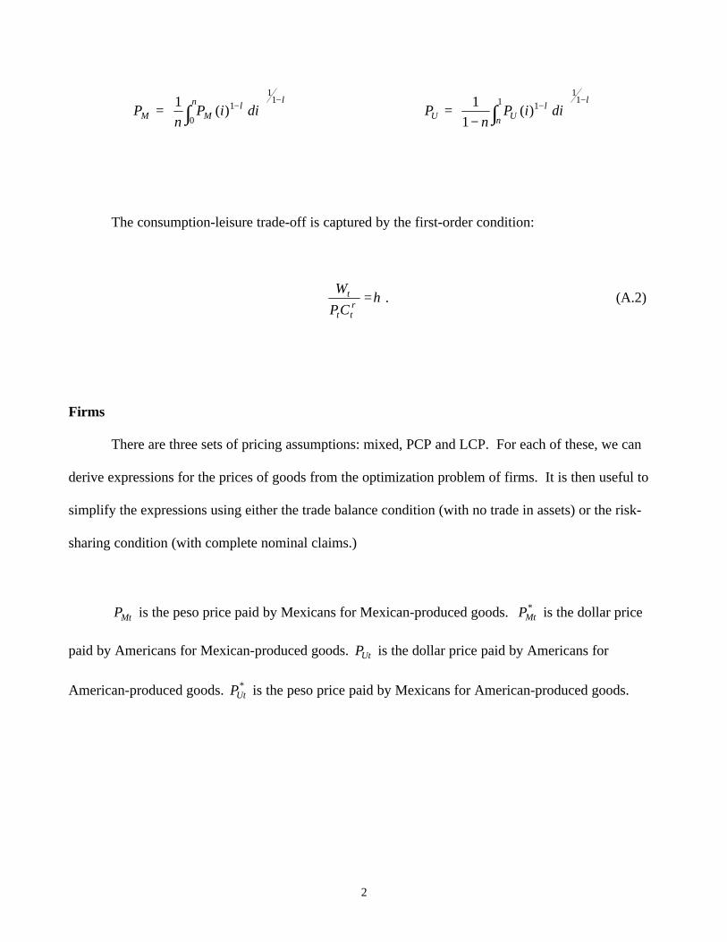
The consumption-leisure trade-off is captured by the first-order condition:

ηρ =tt

t

CP

W. (A.2)

Firms

There are three sets of pricing assumptions: mixed, PCP and LCP. For each of these, we can

derive expressions for the prices of goods from the optimization problem of firms. It is then useful to

simplify the expressions using either the trade balance condition (with no trade in assets) or the risk-

sharing condition (with complete nominal claims.)

MtP is the peso price paid by Mexicans for Mexican-produced goods. *MtP is the dollar price

paid by Americans for Mexican-produced goods. UtP is the dollar price paid by Americans for

American-produced goods. *UtP is the peso price paid by Mexicans for American-produced goods.

3

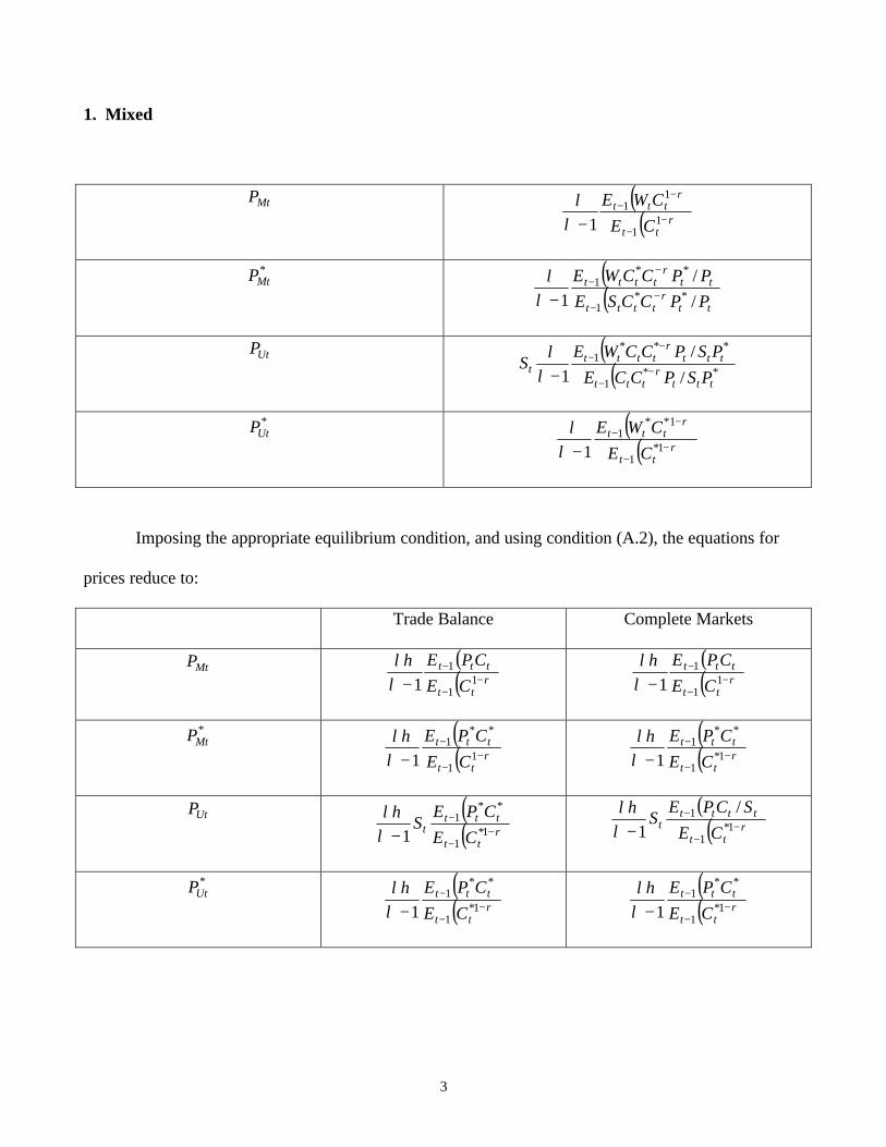
1. Mixed

MtP ( )( )ρ

ρ

λλ

−−

−−

− 11

11

1 tt

ttt

CE

CWE

*MtP ( )

( )tttttt

tttttt

PPCCSE

PPCCWE

/

/

1 **1

**1

ρ

ρ

λλ

−−

−−

−

UtP ( )( )**

1

***1

/

/

1 tttttt

tttttttt

PSPCCE

PSPCCWES ρ

ρ

λλ

−−

−−

−

*UtP ( )

( )ρ

ρ

λλ

−−

−−

− 1*1

1**1

1 tt

ttt

CE

CWE

Imposing the appropriate equilibrium condition, and using condition (A.2), the equations for

prices reduce to:

Trade Balance Complete Markets

MtP ( )( )ρλ

λη−

−

−

− 11

1

1 tt

ttt

CE

CPE ( )( )ρλ

λη−

−

−

− 11

1

1 tt

ttt

CE

CPE

*MtP ( )

( )ρλλη

−−

−

− 11

**1

1 tt

ttt

CE

CPE ( )( )ρλ

λη−

−

−

− 1*1

**1

1 tt

ttt

CE

CPE

UtP ( )( )ρλ

λη−

−

−

− 1*1

**1

1 tt

tttt

CE

CPES

( )( )ρλ

λη−

−

−

− 1*1

1 /

1 tt

ttttt

CE

SCPES

*UtP ( )

( )ρλλη

−−

−

− 1*1

**1

1 tt

ttt

CE

CPE ( )( )ρλ

λη−

−

−

− 1*1

**1

1 tt

ttt

CE

CPE

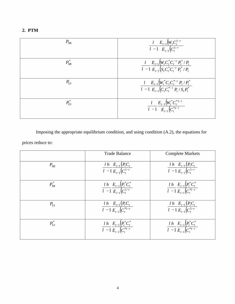
4

2. PTM

MtP ( )( )ρ

ρ

λλ

−−

−−

− 11

11

1 tt

ttt

CE

CWE

*MtP ( )

( )tttttt

tttttt

PPCCSE

PPCCWE

/

/

1 **1

**1

ρ

ρ

λλ

−−

−−

−

UtP ( )( )**

1

***1

/

/

1 tttttt

tttttt

PSPCCE

PPCCWEρ

ρ

λλ

−−

−−

−

*UtP ( )

( )ρ

ρ

λλ

−−

−−

− 1*1

1**1

1 tt

ttt

CE

CWE

Imposing the appropriate equilibrium condition, and using condition (A.2), the equations for

prices reduce to:

Trade Balance Complete Markets

MtP ( )( )ρλ

λη−

−

−

− 11

1

1 tt

ttt

CE

CPE ( )( )ρλ

λη−

−

−

− 11

1

1 tt

ttt

CE

CPE

*MtP ( )

( )ρλλη

−−

−

− 11

**1

1 tt

ttt

CE

CPE ( )( )ρλ

λη−

−

−

− 1*1

**1

1 tt

ttt

CE

CPE

UtP ( )( )ρλ

λη−

−

−

− 1*1

1

1 tt

ttt

CE

CPE ( )( )ρλ

λη−

−

−

− 11

1

1 tt

ttt

CE

CPE

*UtP ( )

( )ρλλη

−−

−

− 1*1

**1

1 tt

ttt

CE

CPE ( )( )ρλ

λη−

−

−

− 1*1

**1

1 tt

ttt

CE

CPE

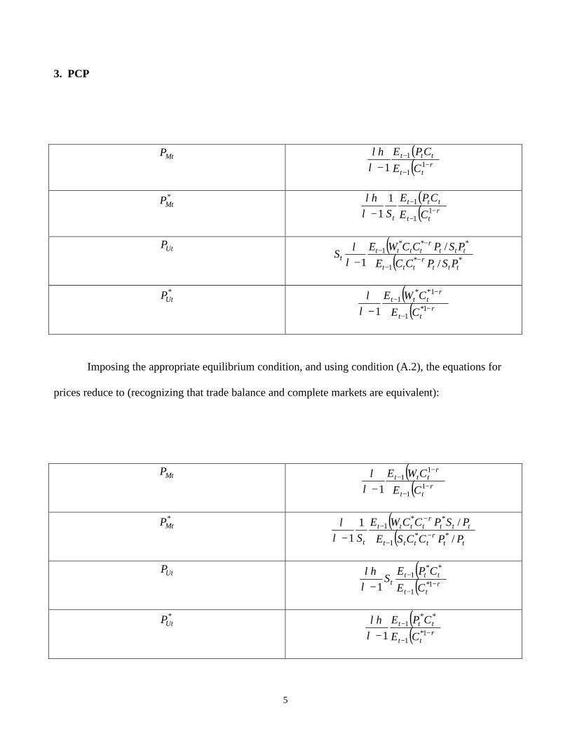
5

3. PCP

MtP ( )( )ρλ

λη−

−

−

− 11

1

1 tt

ttt

CE

CPE

*MtP ( )

( )ρλλη

−−

−

− 11

11

1 tt

ttt

t CE

CPE

S

UtP ( )( )**

1

***1

/

/

1 tttttt

tttttttt

PSPCCE

PSPCCWES ρ

ρ

λλ

−−

−−

−

*UtP ( )

( )ρ

ρ

λλ

−−

−−

− 1*1

1**1

1 tt

ttt

CE

CWE

Imposing the appropriate equilibrium condition, and using condition (A.2), the equations for

prices reduce to (recognizing that trade balance and complete markets are equivalent):

MtP ( )( )ρ

ρ

λλ

−−

−−

− 11

11

1 tt

ttt

CE

CWE

*MtP ( )

( )tttttt

ttttttt

t PPCCSE

PSPCCWE

S /

/1

1 **1

**1

ρ

ρ

λλ

−−

−−

−

UtP ( )( )ρλ

λη−

−

−

− 1*1

**1

1 tt

tttt

CE

CPES

*UtP ( )

( )ρλλη

−−

−

− 1*1

**1

1 tt

ttt

CE

CPE

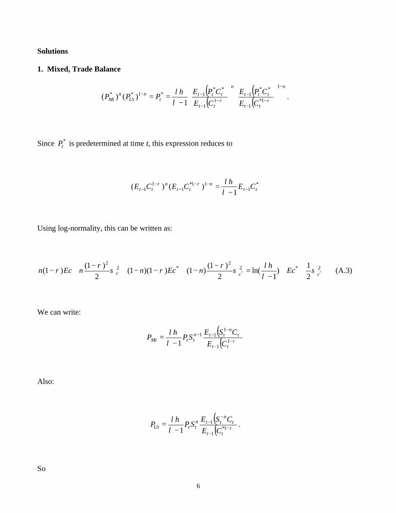
6

Solutions

1. Mixed, Trade Balance

( )( )

( )( )

n

tt

ttt

n

tt

tttt

nUt

nMt

CE

CPE

CE

CPEPPP

−

−−

−−

−

−−

−

==1

1*1

**1

11

**1*1**

1)()( ρρλ

λη.

Since *tP is predetermined at time t, this expression reduces to

*1

11*1

11 1

)()( ttn

ttn

tt CECECE −−−

−−

− −=

λληρρ

Using log-normality, this can be written as:

2*22

*22

**

2

1)

1ln(

2

)1()1()1)(1(

2

)1()1( ccc EcnEcnnEcn σ

λλη

σρ

ρσρ

ρ ++−

=−

−+−−+−

+− (A.3)

We can write:

( )( )ρλ

λη−

−

−−−

−=

11

111

1 tt

tn

ttnttMt

CE

CSESPP

Also:

( )( )ρλ

λη−

−

−−

−=

1*1

1

1 tt

tn

ttnttUt

CE

CSESPP .

So

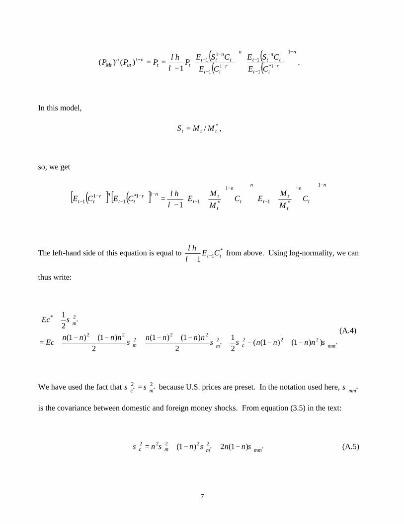
7

( )( )

( )( )

n

tt

tn

tt

n

tt

tn

tttt

nut

nMt

CE

CSE

CE

CSEPPPP

−

−−

−−

−−

−−−

−

==1

1*1

11

1

111

1)()( ρρλ

λη.

In this model,

*/ ttt MMS = ,

so, we get

( )[ ] ( )[ ]n

t

n

t

tt

n

t

n

t

tt

n

tt

n

tt CM

MEC

M

MECECE

−−

−

−

−−−

−−

−

−

=

1

*1

1

*1

11*1

11 1λ

ληρρ

The left-hand side of this equation is equal to *11 tt CE −−λ

λη from above. Using log-normality, we can

thus write:

**

*

))1()1((2

1

2

)1()1(

2

)1()1(

2

1

222222

222

2*

mmcmm

m

nnnnnnnnnnnn

Ec

Ec

σσσσ

σ

−+−−+−+−

+−+−

+=

+(A.4)

We have used the fact that 22** mc σσ = because U.S. prices are preset. In the notation used here, *mmσ

is the covariance between domestic and foreign money shocks. From equation (3.5) in the text:

** )1(2)1( 22222mmmmc nnnn σσσσ −+−+= (A.5)

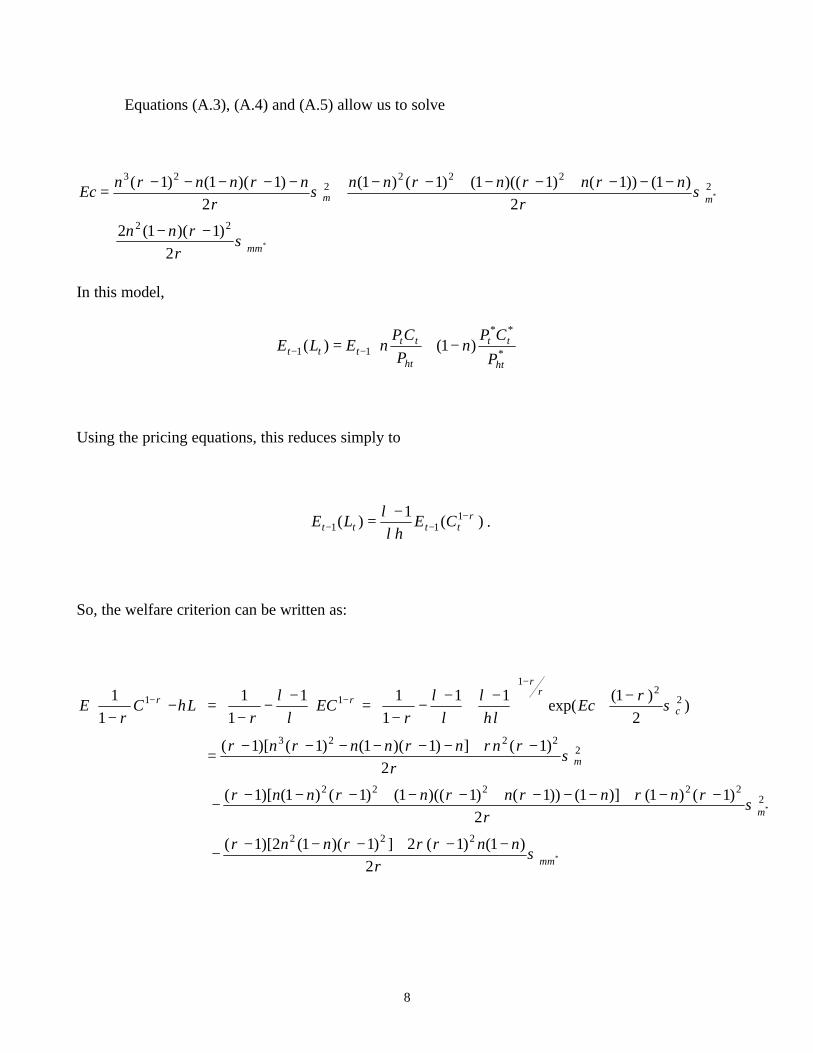
8

Equations (A.3), (A.4) and (A.5) allow us to solve

*

*

2

)1)(1(2

2

)1())1()1)((1()1()1(

2

)1)(1()1(

22

2222

223

mm

mm

nn

nnnnnnnnnEc

σρ

ρ

σρ

ρρρσ

ρρρ

−−+

−−−+−−+−−+

−−−−−=

In this model,

−+= −− *

**

11 )1()(ht

tt

ht

ttttt

P

CPn

P

CPnELE

Using the pricing equations, this reduces simply to

)(1

)( 111

ρ

ληλ −

−−−

= tttt CELE .

So, the welfare criterion can be written as:

*

*

2

)1()1(2])1)(1(2)[1(

2

)1()1()]1())1()1)((1()1()1()[1(

2

)1(])1)(1()1()[1(

)2

)1(exp(

11

1

11

1

1

1

1

222

222222

22223

22

1

11

mm

m

m

c

nnnn

nnnnnn

nnnnn

EcECLCE

σρ

ρρρρ

σρ

ρρρρρρ

σρ

ρρρρρ

σρ

ηλλ

λλ

ρλλ

ρη

ρ

ρρ

ρρ

−−+−−−−

−−+−−−+−−+−−−−

−+−−−−−−=

−+

−

−−

−=

−−

−=

−

−

−

−−

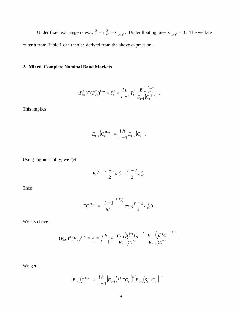
9

Under fixed exchange rates, **22

mmmm σσσ == . Under floating rates 0* =mmσ . The welfare

criteria from Table 1 can then be derived from the above expression.

2. Mixed, Complete Nominal Bond Markets

( )( )ρλ

λη−

−

−−

−==

1*1

*1**1**

1)()(

tt

tttt

nUt

nMt

CE

CEPPPP .

This implies

( ) ( )*1

1*1 1 tttt CECE −

−− −

=λληρ .

Using log-normality, we get

22***

2

2

2

2mcEc σ

ρσ

ρ −=

−=

Then

)2

1exp(

1 2

1

1**mEC σ

ρηλ

λ ρρ

ρ −

−=

−

− .

We also have

( )( )

( )( )

n

tt

tn

tt

n

tt

tn

tttt

nut

nMt

CE

CSE

CE

CSEPPPP

−

−−

−−

−−

−−−

−

==1

11

11

1

111

1)()( ρρλ

λη.

We get

( ) ( )[ ] ( )[ ] n

tn

tt

n

tn

tttt CSECSECE−−

−−

−−

− −=

1

11

11

1 1λληρ .

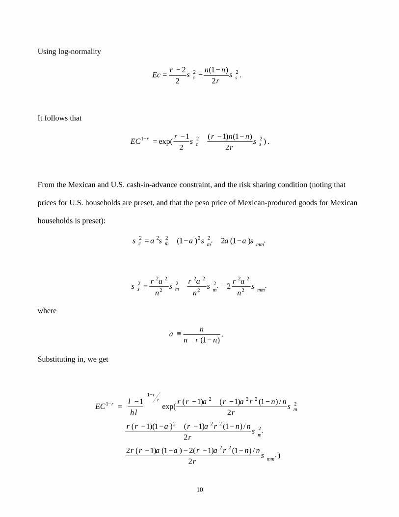
10

Using log-normality

22

2

)1(

2

2sc

nnEc σ

ρσ

ρ −−

−= .

It follows that

)2

)1()1(

2

1exp( 221

scnn

EC σρ

ρσ

ρρ −−+

−=− .

From the Mexican and U.S. cash-in-advance constraint, and the risk sharing condition (noting that

prices for U.S. households are preset, and that the peso price of Mexican-produced goods for Mexican

households is preset):

** )1(2)1( 22222mmmmc σαασασασ −+−+=

** 2

222

2

222

2

222 2 mmmms

nnnσ

αρσ

αρσ

αρσ −+=

where

)1( nn

n

−+≡

ρα .

Substituting in, we get

)2

/)1()1(2)1()1(2

2

/)1()1()1)(1(

2

/)1()1()1(exp(

1

*

*

22

2222

2222

1

1

mm

m

m

nn

nn

nnEC

σρ

ραρααρρ

σρ

ραραρρ

σρ

ραραρρηλ

λ ρρ

ρ

−−−−−+

−−+−−+

−−+−

−=

−

−

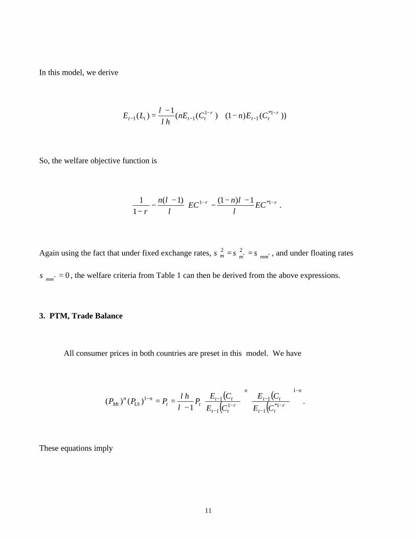
11

In this model, we derive

))()1()((1

)( 1*1

111

ρρ

ληλ −

−−

−− −+−

= tttttt CEnCnELE

So, the welfare objective function is

ρρ

λλ

λλ

ρ−− −−

−

−−

−1*1 1)1()1(

1

1EC

nEC

n.

Again using the fact that under fixed exchange rates, **22

mmmm σσσ == , and under floating rates

0* =mmσ , the welfare criteria from Table 1 can then be derived from the above expressions.

3. PTM, Trade Balance

All consumer prices in both countries are preset in this model. We have

( )( )

( )( )

n

tt

tt

n

tt

tttt

nUt

nMt

CE

CE

CE

CEPPPP

−

−−

−−

−

−−

−

==1

1*1

11

1

11

1)()( ρρλ

λη.

These equations imply

12

( )[ ] ( )[ ] ( )tt

n

tt

n

tt CECECE 1

11*1

11 1 −

−−−

−− −

=λληρρ .

Similarly

( )[ ] ( )[ ] ( )*1

11*1

11 1 tt

n

tt

n

tt CECECE −−−

−−

− −=

λληρρ .

From these, we obtain

−++=

−+−−+

−+−

1ln

2

1)

2

)1()1)((1()

2

)1()1(( 22

2*2

2

*

λλη

σσρ

ρσρ

ρ mmm EcEcnEcn

−++=

−+−−+

−+−

1ln

2

1)

2

)1()1)((1()

2

)1()1(( 2*2

2*2

2

**

λλη

σσρ

ρσρ

ρ mmm EcEcnEcn .

Here we have used the fact that in this model 22mc σσ = and 22

** mc σσ = . Solving these we get

)2

)1)(1(

2

))1)(1(1)(1(exp(

1 22

2

1

1*mm

nnEC σ

ρσ

ρρηλ

λ ρρ

ρ −−−

−−+−

−=

−

− .

Again in this model

)(1

)( 111

ρ

ληλ −

−−−

= tttt CELE

So the welfare expression is given by

13

ρρ

λλ

ρη

ρ−−

−−

−=

−

−11 1

1

1

1

1ECLCE

We can arrive at the welfare criteria for fixed versus floating (reported in Table 1) just as in the

previous cases. In particular, we find simply that floating rates are preferred to fixed rates when

22*mm σσ < .

4. PTM, Complete Nominal Bond Markets

Here we have

( )( )

( )( )

n

tt

tt

n

tt

tttt

nUt

nMt

CE

CE

CE

CEPPPP

−

−−

−−

−

−−

−

==1

11

11

1

11

1)()( ρρλ

λη,

so

( ) ( )tttt CECE 11

1 1 −−

− −=

λληρ .

Similarly,

( ) ( )*1

1*1 1 tttt CECE −

−− −

=λληρ .

We can solve these to find

)2

1exp(

1 2

1

1mEC σ

ρηλ

λ ρρ

ρ −

−=

−

−

and

)2

1exp(

1 2

1

1**mEC σ

ρηλ

λ ρρ

ρ −

−=

−

− ,

14

where we have used the fact that in this model 22mc σσ = and 22

** mc σσ = . Since in this model

))()1()((1

)( 1*1

111

ρρ

ληλ −

−−

−− −+−

= tttttt CEnCnELE ,

we have the utility term is:

ρρ

λλ

λλ

ρ−− −−

−

−−

−1*1 1)1()1(

1

1EC

nEC

n.

We arrive at the results in Table 1 as in the previous sections.

5. PCP

As in case 4, we get

( )( )

( )( )

n

tt

tn

tt

n

tt

tn

tttt

nut

nMt

CE

CSE

CE

CSEPPPP

−

−−

−−

−−

−−−

−

==1

11

11

1

111

1)()( ρρλ

λη

which implies

( ) ( )[ ] ( )[ ] n

tn

tt

n

tn

tttt CSECSECE−−

−−

−−

− −=

1

11

11

1 1λληρ ,

and thus

)2

)1()1(

2

1exp( 221

scnn

EC σρ

ρσ

ρρ −−+

−=− .

Since in this model */ ttt MMS = and *tt CC = , we have

** )1(2)1( 22222mmmmc nnnn σσσσ −+−+=

and

** 2222mmmms σσσσ −+= .

15

Plugging in, we get

)2

)1()1(2)1()1(2

2

)1()1()1)(1(

2

)1()1()1(exp(

1

*

*2

2

22

1

1

mm

m

m

nnnn

nnn

nnnEC

σρ

ρρρ

σρ

ρρρ

σρρρρ

ηλλ ρ

ρ

ρ

−−−−−+

−−+−−+

−−+−

−=

−

−

Also, since *tt CC = ,

)(1

)( 111

ρ

ληλ −

−−−

= tttt CELE

and the welfare criterion reduces to maximizing

ρρ

λλ

ρη

ρ−−

−−

−=

−

−11 1

1

1

1

1ECLCE .

Using the expressions above, we arrive at the welfare criteria presented in Table 1.