Optimal dynamic control of invasions: applying a

Ecological Applications, 25(4), 2015, pp. 1131–1141� 2015 by the Ecological Society of America

Optimal dynamic control of invasions: applying a systematicconservation approach

VANESSA M. ADAMS1

AND SAMANTHA A. SETTERFIELD

Research Institute for the Environment and Livelihoods and National Environmental Research Program Northern Australia Hub,Charles Darwin University, Darwin, NT 0909 Australia

Abstract. The social, economic, and environmental impacts of invasive plants are wellrecognized. However, these variable impacts are rarely accounted for in the spatialprioritization of funding for weed management. We examine how current spatially explicitprioritization methods can be extended to identify optimal budget allocations to botheradication and control measures of invasive species to minimize the costs and likelihood ofinvasion. Our framework extends recent approaches to systematic prioritization of weedmanagement to account for multiple values that are threatened by weed invasions with amulti-year dynamic prioritization approach. We apply our method to the northern portion ofthe Daly catchment in the Northern Territory, which has significant conservation values thatare threatened by gamba grass (Andropogon gayanus), a highly invasive species recognized bythe Australian government as a Weed of National Significance (WONS). We interfaceMarxan, a widely applied conservation planning tool, with a dynamic biophysical model ofgamba grass to optimally allocate funds to eradication and control programs under twobudget scenarios comparing maximizing gain (MaxGain) and minimizing loss (MinLoss)optimization approaches. The prioritizations support previous findings that a MinLossapproach is a better strategy when threats are more spatially variable than conservationvalues. Over a 10-year simulation period, we find that a MinLoss approach reduces futureinfestations by ;8% compared to MaxGain in the constrained budget scenarios and ;12% inthe unlimited budget scenarios. We find that due to the extensive current invasion and rapidrate of spread, allocating the annual budget to control efforts is more efficient than fundingeradication efforts when there is a constrained budget. Under a constrained budget, applyingthe most efficient optimization scenario (control, minloss) reduces spread by ;27% comparedto no control. Conversely, if the budget is unlimited it is more efficient to fund eradicationefforts and reduces spread by ;65% compared to no control.

Key words: Andropogon gayanus; connectivity; invasive species management; Marxan; scheduling;systematic conservation planning; vulnerability.

INTRODUCTION

The impact of invasive species on natural values can

be significant including alteration of ecosystem processes

and species composition (Ehrenfeld 2010). Invasive

species are often listed as a threat to biodiversity and

have been linked to species extinctions (Kingsford et al.

2009, Butchart et al. 2010). While the risks of invasive

species to biodiversity are recognized, effective control

or eradication programs may require long periods of

funding with large associated costs and there are limited

budgets to support such actions (Panetta 2007, Simberl-

off 2009, Panetta et al. 2011).

Given that environmental damages caused by invasive

species can be significant (Pimentel et al. 2005), it is

critical to allocate limited financial resources carefully.

Yet, despite the widespread acceptance of systematic

conservation approaches around the world, and the

demonstrated cost effectiveness and accountability of

these methods, application to regional weed manage-

ment has only just begun (Januchowski-Hartley et al.

2011). Januchowski-Hartley et al. (2011) demonstrated

the financial benefits of using a spatially explicit

planning framework and accounting for the variable

costs of different actions. However, this study was

limited to a single time step, with the authors

highlighting the need to extend this approach to a

multi-year scheduling approach.

Limited resources require managers to schedule

management actions across space and time (Possingham

et al. 2009), but systematic approaches to scheduling

optimal location of control efforts are limited (Epan-

chin-Niell and Wilen 2012). Two iterative heuristics

commonly applied to scheduling problems include

minimizing loss (MinLoss), which prioritizes sites that

are both important for meeting objectives and likely to

be lost without intervention, and maximizing gain

(MaxGain), which prioritizes sites only based on values

Manuscript received 4 June 2014; revised 17 October 2014;accepted 22 October 2014. Corresponding Editor: R. A.Hufbauer

1 E-mail: [email protected]

1131

contributing to objectives and not whether the site is

under threat or not. Studies have found that MinLossoutperforms MaxGain for retaining conservation fea-

tures when habitat loss is considered (Wilson et al.2006). It has been demonstrated that high habitat-loss

rates can amplify the differences between good and poorapproaches to scheduling management actions (Presseyet al. 2004, Visconti et al. 2010a, b). Given invasive

species can have high rates of spread, previous researchfindings suggest that a MinLoss approach may outper-

form a MaxGain approach to scheduling invasivemanagement when spread is considered.

Scheduling management of invasive species requiresan understanding of the spatial distribution of infesta-

tions through time as well as the variable costs andbenefits of management (Epanchin-Niell and Hastings

2010, Epanchin-Niell and Wilen 2012). We build uponthe framework presented by Januchowski-Hartley et al.

(2011) by extending the decision making process from asingle time step to a multi-year scheduling problem and

explore the performance of these two heuristics. Weaddress the following two research questions: (1) Is

minimizing loss better than maximizing gain when thespatial spread of the invasive species is considered? (2)

Does eradication or control perform best under con-strained and unconstrained budgets?

Based on our results, we provide recommendationsfor optimal scheduling of management actions and

demonstrate the utility of a multi-year dynamic ap-proach.

METHODS

Study species

Invasive grasses, such as the African grass Andropo-

gon gayanus Kunth. (gamba grass), pose a major threatto savannas (Brooks et al. 2004, Setterfield et al. 2010).

Gamba grass is a perennial C4 grass that forms largetussocks in excess of 3 m high and displaces the much

shorter native vegetation (Brooks et al. 2010). Gambagrass is one of five species of tropical invasive grasses

that have been listed as a national Key ThreateningProcess (KTP) for Australia and has recently been listedas an Australian Weed of National Significance

(WONS). Significant ecological impacts result fromgamba grass invasions including increases in fire severity

leading to a reduction in tree canopy and severe impactson the understory (Rossiter et al. 2003, Brooks et al.

2010, Setterfield et al. 2010). Rapid spread of gambagrass has been observed from initial source paddocks in

northern Australia and suggests explosive rates ofspread analogous to highly invasive plants elsewhere.

Modelling predicts that most of Australia’s mesicsavanna is suitable for invasion, including ;380 000

km2 of the Australia’s Northern Territory (NorthernTerritory Government 2009), as well as large savanna

areas in Queensland and Western Australia (Hutley andSetterfield 2008). The current known area of gamba

grass infestations in the Northern Territory extends

south approximately 350 km from Darwin to Katherine

in the Daly River Catchment. It is estimated that gamba

grass covers 1–1.5 million ha of the Northern Territory

(DLRM 2014) and is abundant in the Darwin rural

region including a core infestation in Litchfield National

Park (;100 km south of Darwin).

Study region

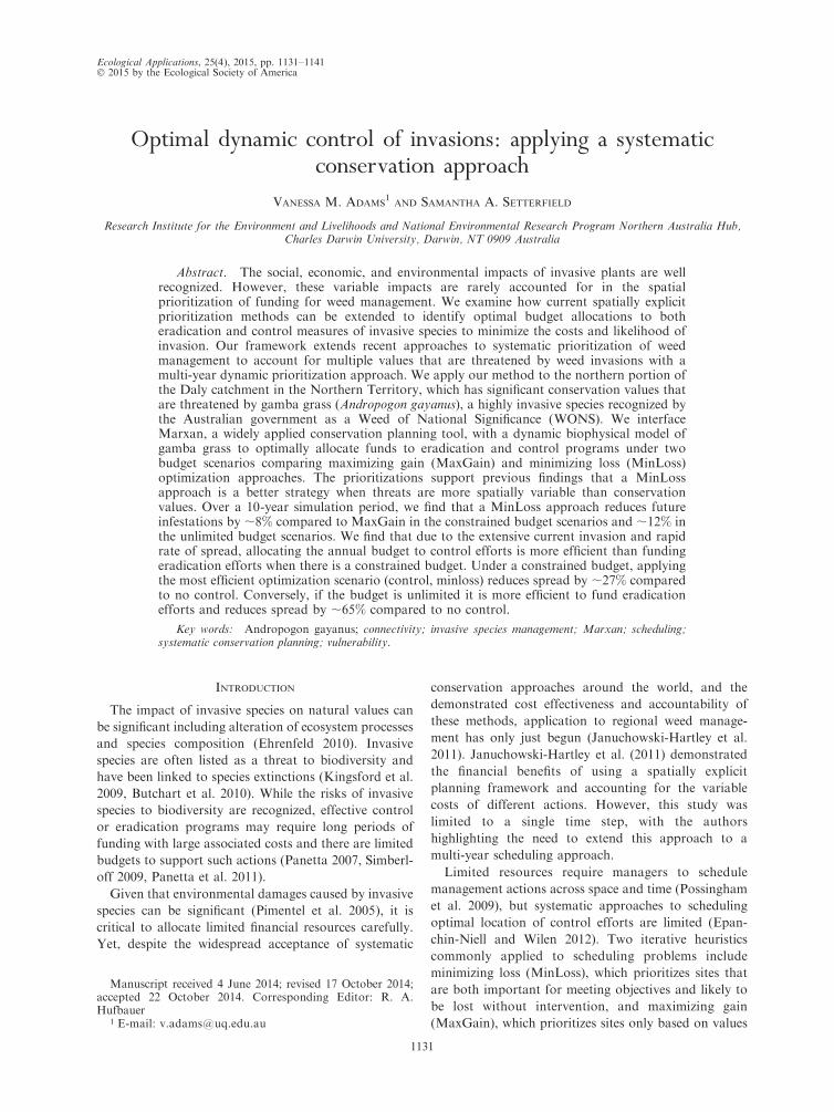
We select our study region to include key environ-

mental assets with significant gamba grass infestations,

such as Litchfield National Park. The study region

covers ;1.2 million ha and includes the northernmost

portion of the Daly catchment, which encompasses

Litchfield National Park as well as the Daly River (Fig.

1). The Daly catchment is a priority for both develop-

ment and conservation, with notable features such as the

Daly River, one of northern Australia’s largest rivers

with unusually consistent year-round flow, extensive

gallery (rainforest) vegetation, and five recognized sites

of conservation significance (NRETAS 2009). We

consider seven conservation features that are high

priority for gamba grass management including the

protected areas region in Litchfield, which is recognized

for high biodiversity (biodiversity zone), a region in

Litchfield recognized for its tourism sites (tourist zone),

rainforest vegetation, and three sites of conservation

significance (Anson Bay and associated coastal flood-

plains, Finnis River coastal floodplain, and Daly River

middle reaches). Within the study region, there are seven

significant stakeholders who control 99% of the land

area including managers of national parks, aboriginal

land trusts, pastoral properties and crown lease land.

The remaining 1% of land area is held predominantly by

small landholders with an average parcel size of 150 ha.

Aerial surveys for the region provide a distribution map

of infestations; however, we updated the existing aerial

survey data to include other survey data provided by

local property managers to provide a more comprehen-

sive distribution map.

Planning units

The current distribution of gamba grass infestations

for the Northern Territory was developed based on a

250-m grid for the region (Petty et al. 2012). We

therefore create a uniform 250-m grid across our study

region (n¼ 313 544) to be consistent with existing maps

and models available for gamba grass. We use the 6.25-

ha cells as our planning units and calculate the costs and

benefits of managing the infestation in each grid cell

separately.

Simulation approach

We extended the recent approaches to systematic

prioritization of weed management (Januchowski-Hart-

ley et al. 2011) to a multi-year scheduling problem. We

set explicit objectives for management of gamba grass

taking into account spatially heterogeneous environ-

mental values. We followed the framework detailed by

VANESSA M. ADAMS AND SAMANTHA A. SETTERFIELD1132 Ecological ApplicationsVol. 25, No. 4

Adams and Setterfield (2012) for designing multi-year

weed management programs as described here. For each

year we simulate growth and spread of gamba grass and

management of gamba grass in the study region. The

simulation annual cycle followed these steps: (1) Select

planning units for management. We consider two

budget scenarios. For each budget scenario we select

planning units until the budget is exhausted. (2)

Simulate gamba grass spread. (3) Simulate gamba grass

density growth. (4) Update maps for selection strategy.

At the end of each annual time step we update the map

of gamba grass available for management, calculate the

costs of eradication and control (which are a function of

size and density of infestation and year of treatment),

and update the vulnerability matrix (used for the

MinLoss strategy).

We interfaced Marxan (for selection of planning units

in step 1) to our dynamic biophysical model (steps 2–4)

using Matlab (R2012b, Version 8.0; MathWorks,

Natick Massachusetts, USA).

Each simulation is run for 10 years to reflect a 10-year

management plan for gamba grass. We also run the

simulation in the absence of any management for 10

years and consider this the baseline. The performance of

each simulation is measured with several criteria. First,

we calculate the total spread prevented across the full

study region regardless of conservation status as the

final area infested in the baseline of no management

minus the final area infested in the management

scenario. We also record the present value of expendi-

tures using a 5% discount rate for each scenario and

calculate the cost of avoided infestations as the present

value divided by total spread prevented. Last, for each

conservation feature in the final time step of each

scenario, we record the total area that is infested and not

being managed, the total area under active management

(control of eradication) and the total area that was

eradicated during the 10-year management period and is

clean in the final time step. Lastly, we consider two static

scenarios in which a one-off investment is provided for

complete management of all infestations regardless of

conservation status and calculate the present value of

management costs for control and eradication as well as

the avoided infestations and cost of avoided infestations.

FIG. 1. Study area in the northwest portion of the Daly Catchment, Australia. On the left, the Daly Catchment cadastre,national parks, and rivers are shown to provide regional context. The inset shows the Australian states in gray, Northern Territoryin white, and the Daly catchment in black. On the right, the study region is shown enlarged with conservation features: sites ofconservation significance, rainforest galleries, protected areas, high biodiversity value region in Litchfield, and high tourism valueregion in Litchfield. Mapped gamba grass infestations identified from aerial surveys are shown in black.

June 2015 1133DYNAMIC CONTROL OF INVASIONS

Scenario design

When selecting planning units for management (step

1) we consider two potential management actions: local

control and local eradication of gamba grass infesta-

tions. Local control is defined as the management of

gamba grass to prevent spread and prevent further

increases in size and density and includes actions such as

chemical treatment of the boundaries of infestations.

Control efforts must occur in perpetuity in order to

effectively stop increases in size of gamba grass

infestations. Local eradication of gamba grass is defined

as the total elimination (including accumulated seed

bank) of gamba grass within a planning unit through

intense chemical treatment of the infestation over a

timeframe of 6–8 years depending on the size and

density (for details, see Adams and Setterfield 2013). We

consider two scheduling approaches: MaxGain and

MinLoss. In the context of invasive species manage-

ment, MaxGain is similar to asset recovery in that

infested planning units that are important to meeting

objectives will be prioritized, while MinLoss will

prioritize both asset recovery and prevention by

selecting infested planning units of high priority and

planning units that threaten important assets.

Combining the two scheduling approaches with the

two management actions results in four scheduling

scenarios: scenario 1, MinLoss and local control;

scenario 2, MaxGain and local control; scenario 3,

MinLoss and local eradication; scenario 4, MaxGain

and local eradication.

Biophysical model of gamba grass growth, spread,

and control

We model the growth of gamba grass as a determin-

istic increase in the density class of each infested

planning unit. The deterministic growth model as a

function of time since first infested is

dðtÞ ¼1; t � 7

2; 7 , t � 11

3; t . 11

8<:

where density class 1 is scattered infestation (,10%cover), 2 is medium infestation (10–50% cover) and 3 is

dense infestation (.50% cover). The deterministic

growth model is based on discussions with experts

(scientists and land managers highly familiar with

gamba grass) and examination of a time series of aerial

photographs.

We adapted the spread model approach presented by

Williams et al. (2008), which combines dispersal

direction based on cardinal direction from wind data,

dispersal distance using a negative exponential distri-

bution and habitat suitability to constrain establish-

ment; we simulated spread events stochastically using

this parameterization as opposed to estimating prob-

ability of infestation at a site (for a similar application

see Steel et al. 2014). Thus, for each time step the

number of spread events from a planning unit was

estimated using a Poisson distribution (the Poisson

distribution is a commonly applied count distribution

for estimating fecundity, e.g., see Buckley et al. [2005]),

distance of each spread event was estimated using a

negative exponential distribution, direction of each

spread event was estimated using a cardinal direction

distribution and establishment in a new planning unit

was constrained by habitat suitability. We estimated

spread rate based on historic distribution (mean

number of spread events estimated to be 50 based on

historic and current distribution of gamba grass taking

into account average suitability in the region). We used

a published mean spread distance of 500 m (Petty et al.

2012). We estimated the cardinal direction distribution

based on the approach presented by Steel et al. (2014)

where the proportion of wind blowing in each direction

during time of seeding (June–July) was recorded based

on data from the Bureau of Meteorology (prevailing

south easterly winds). We constrained establishment in

planning units using modelled habitat suitability (see

Appendix). To reflect the known biology of gamba

grass, infested cells had to reach an age of 7 years in

order to spread (based on known reproduction time of

a minimum of 2 years of age and investigation of aerial

photos in which new infestations were only detected

after neighboring infestations were approximately 7

years old).

We assume that once a planning unit is selected for

control or eradication that it does not grow or spread.

We also assume that once a planning unit is selected for

management, it must remain under management for the

duration of the simulation (for control) or until the

management time period is completed (for eradication,

5–7 years depending on initial density) (for more details,

see Adams and Setterfield 2013). For eradication we

assume that density is decreasing over the time period

such that at the end of the treatment period the planning

unit is uninfested (costs are therefore time dependent,

see Cost of control and eradication).

Cost of control and eradication

We model the costs of gamba grass management using

control and eradication cost models developed by

Adams and Setterfield (2013). The cost models are a

function of infestation size, density, and year of

treatment. We define infestations as each planning unit

that is infested. This neglects that neighboring planning

units may be managed as a single infestation. Therefore

our estimated costs do not take advantage of economies

of scale of managing larger infestations, but we consider

this approach to be conservative given different land

managers may define infestations and approach man-

agement in different ways. All costs are therefore

calculated for each planning unit based on the density

class in the relevant time step and a size of 6.25 ha (250-

m grid planning units).


Management action selection strategies

We test our four different strategies for allocating

management actions under two budget scenarios. The

first budget scenario applies a constrained annual

budget of AUD$600 000 (AUD, Australian dollars)

and the second budget scenario allows an unlimited

annual budget. The annual budget of AUD$600 000 was

selected to reflect budgets received by other parks for

strategic weed management programs of high threat

species (e.g., Kakadu Mimosa team annual cost of

AUD$500 000; DEH 2004) and to reflect the likely costs

of fire management associated with regional gamba

grass infestations if there is no immediate investment in

a management program (AUD$550 000 in fire manage-

ment costs estimated for 2013 in Batchelor region;

Setterfield et al. 2014). Each of the four strategies has a

unique objective function. The objective function for all

four scenarios aims to jointly minimize the cost of

management of infestations, minimize the probability of

re-infestation of managed infestations, and meet the

targets set for management of conservation values.

Therefore each objective function contains three math-

ematical components: (1) the cost of managing the

planning units selected (ci ); (2) probability of infesta-

tion; (3) target penalty, which is equal to the cost of

raising a feature up to its target representation level.

The first two components of the equation are the same

for both the MaxGain and MinLoss strategies. We vary

the calculation of the targets and target penalty (the

third component of the equation) to produce a

MaxGain and MinLoss strategy: the MaxGain strategy

accounts for those conservation features currently

infested while the MinLoss strategy also accounts for

those conservation features that are vulnerable to

infestation. For the MaxGain strategies, we set a target

t of 100% for all conservation features j that are

currently infested Cj. This means that we want to

manage 100% of infestations within all identified

conservation features (i.e., the protected areas region

in Litchfield, Litchfield tourism zone, Litchfield biodi-

versity zone, rainforest galleries, and sites of conserva-

tion significance). Any infestations that are not within

conservation features are not targeted for on ground

management under the MaxGain objective function.

For the MinLoss strategies, in addition to the targets for

currently infested features, we also set a target t of 100%of the expected features at risk (CRj) expressed as

CRj ¼XNs

i¼1

XNs

h¼1

vihajh

where Ns is the number of planning units, vih is the

vulnerability of planning unit h due to spread from

planning unit i (calculated as the probability of spread

from i to h from the spread model) and ajh is the amount

of feature j in planning unit h. Any infestations that are

not within conservation features are not targeted for

management under the MinLoss objective function

unless they are within spread distance to a conservation

feature.

We minimize each objective function with the Marxan

software (Ball et al. 2009). Marxan uses a simulated

annealing algorithm to find good solutions to the

generalized objective function

minimize

XNs

i¼1

xici þ b

XNs

i

XNs

h

xið1� xhÞcvih

þXNf

j

FPFjFRjHðgjÞgj

tj

� �

where xi is a control variable with value 1 for selected

planning units and 0 for units not selected, ci is the cost

of planning unit i, Ns is the number of planning units, Nf

is the number of features, and tj is the target level for

feature j (Ball et al. 2009). The first part of the equation

minimizes the penalties associated with the cost of the

network and was used in our scenarios to reflect the

variable costs of eradication and control (component 1).

The second part of the equation minimizes the penalties

associated with the configuration or shape of the

network. In our case this part of the equation reflects

our objective to minimize re-infestation of managed

planning units (component 2). The parameter cvihreflects the cost of the connection, in this case the

probability of spread from planning unit i to h

calculated based upon the spread model. The parameter

b, is the boundary length modifier (BLM), a user-defined

variable that controls the importance of minimizing the

total boundary length of the selected areas. For each

scenario, we selected the BLM with the method

described by Stewart and Possingham (2005), intended

to achieve a level of connectivity between selected areas

that does not unduly increase the overall cost of the

solution. The third part of the equation minimizes the

penalties associated with shortfalls in the targets for

each feature (component 3). FPFj is the feature penalty

factor that determines the relative importance of

meeting the representation target for feature j. We apply

a FPF of 10 for all features. FRj is the cost of meeting

the target for feature j starting from no representation in

the reserve network (details in Ball et al. 2009). The

shortfall or gap in management gj for MaxGain is the

unmet representation target calculated as

gj ¼ Cj �XNs

i¼1

xi 3 Cj:

For MinLoss, the shortfall is

gj ¼ CRj �XNs

i¼1

xi 3 CRij

where CRij is the conservation value j at risk from


planning unit i calculated as

CRij ¼XNs

h¼1

vih 3 ajh

This represents the difference in expected conservation

values at risk from gamba grass invasion and thenumber of infestations in conservation features avoided

through management. The Heaviside function, H(g), is astep function taking the value of zero when g¼ 0 and 1

otherwise.

RESULTS

In the initial time step (t ¼ 0), there is 11 000 ha ofinfestations in the study region. In the absence of any

control, over the 10-year period, there is an eightfoldincrease in infestations to 94 000 ha (t¼ 10). In order to

control all initial infestations, an initial annual budget of

AUD$2.4 million is needed, which declines to arecurring annual budget of AUD$1.6 million by year 6

(present value of control of all initial infestations isAUD$13.8 million, Table 1). In order to eradicate all

infestations, an initial annual budget of AUD$6.7million is needed, which declines to AUD$0.5 million

by year 6 (present value of eradicating all initial

infestations is AUD$19.5 million, Table 1).Regardless of on-ground strategy (control or eradi-

cation) or budget, the MinLoss approach outperformedthe MaxGain approach. For example, under the limited

budget scenarios, MinLoss resulted in a ;50% increase

in prevented spread compared to MaxGain (Table 1).

Given a limited budget, it is more effective to fund

control efforts in terms of avoided infestations and cost-

effectiveness (best-performing scenario, MinLoss and

local control; Table 1). If the budget is not limited,

eradication outperforms control and is more effective in

terms of avoided infestations and cost effectiveness (best

performing scenario, MinLoss and local eradication;

Table 1).

In the constrained budget scenarios, the allocation of

budget across conservation features was similar and

reflects the original percentage of features infested

(Table 2). However, the level of management in terms

of total hectares managed was much lower in the local

eradication scenarios (scenarios 3–4) compared to the

local control scenarios (scenarios 1–2) due to the relative

cost of action per ha of eradication. The spatial

allocation of management effort within conservation

features differed between MinLoss and MaxGain

scenarios (Fig. 2), with MinLoss scenarios allocating

more effort to the boundaries of features. These patterns

are visually apparent in the Litchfield infestation: there

are fewer infestations managed under the eradication

scenarios (Fig. 2c, d) compared to control scenarios

(Fig. 2a, b) and MinLoss scenarios (Fig. 2a, c) allocate

more effort to the northwest border of the infestation to

prevent further spread into the biodiversity and tourism

zones.

The unlimited budget allocated effort to all infested

features, resulting in the same patterns of investment

across features for all scenarios. The important differ-

ence between local control and local eradication

TABLE 1. Summary statistics of runs.

Conditions

Total areainfested(ha)

Total 10 yearexpenditure(AUD$)

Total avoidedinfestations

(ha)

Totaleradicatedarea (ha)

Cost of avoidedinfestations(AUD$/ha)

Static estimates for completemanagement

All initial infestations controlled 0 13 815 000 94 000 0 147All initial infestations eradicated 0 19 541 000 94 000 11 000 208

Annual budget $600 000

Scenario 1, MinLoss and local control 69 000 4 635 000 25 000 0 185Scenario 2, MaxGain and local control 77 000 4 637 000 17 000 0 273Scenario 3, MinLoss and local

eradication74 000 4 637 000 20 000 1 300 232

Scenario 4, MaxGain and localeradication

81 000 4 635 000 13 000 1 100 357

Unlimited annual budget

Scenario 1, MinLoss and local control 33 000 12 584 000 61 000 0 206Scenario 2, MaxGain and local control 44 000 10 994 000 50 000 0 220Scenario 3, MinLoss and local

eradication33 000 11 700 000 61 000 8 400 192

Scenario 4, MaxGain and localeradication

44 000 10 154 000 50 000 8 400 203

Notes: The costs and benefits of complete control and eradication are given as static scenarios in addition to summary statisticsfor scenario runs under a constrained annual budget of AUD$600 000 (AUD, Australian dollars) and unlimited annual budget. Foreach run, the total area infested at time step 10 is given, the present value (PV) of expenditures over the 10-year period assuming a5% discount rate, the total avoided infestations in runs where there was management (the baseline no-management final infestationvalue of 94 000 ha is used for calculations), the total infested area that was eradicated in year 10 where there was local eradicationand the cost of avoided infestations (calculated as PV/total avoided infestations). Budget management scenarios are minimizingloss (MinLoss) and maximizing gain (MaxGain).


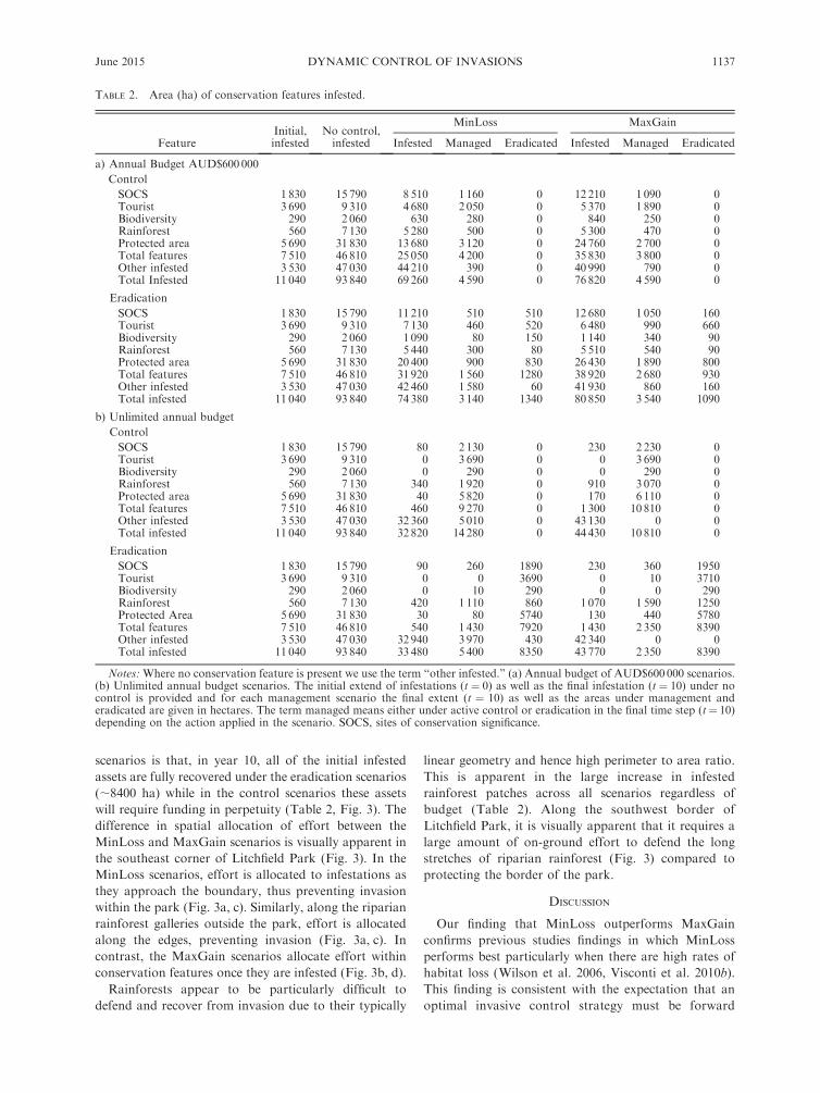
scenarios is that, in year 10, all of the initial infested

assets are fully recovered under the eradication scenarios

(;8400 ha) while in the control scenarios these assets

will require funding in perpetuity (Table 2, Fig. 3). The

difference in spatial allocation of effort between the

MinLoss and MaxGain scenarios is visually apparent in

the southeast corner of Litchfield Park (Fig. 3). In the

MinLoss scenarios, effort is allocated to infestations as

they approach the boundary, thus preventing invasion

within the park (Fig. 3a, c). Similarly, along the riparian

rainforest galleries outside the park, effort is allocated

along the edges, preventing invasion (Fig. 3a, c). In

contrast, the MaxGain scenarios allocate effort within

conservation features once they are infested (Fig. 3b, d).

Rainforests appear to be particularly difficult to

defend and recover from invasion due to their typically

linear geometry and hence high perimeter to area ratio.

This is apparent in the large increase in infested

rainforest patches across all scenarios regardless of

budget (Table 2). Along the southwest border of

Litchfield Park, it is visually apparent that it requires a

large amount of on-ground effort to defend the long

stretches of riparian rainforest (Fig. 3) compared to

protecting the border of the park.

DISCUSSION

Our finding that MinLoss outperforms MaxGain

confirms previous studies findings in which MinLoss

performs best particularly when there are high rates of

habitat loss (Wilson et al. 2006, Visconti et al. 2010b).

This finding is consistent with the expectation that an

optimal invasive control strategy must be forward

TABLE 2. Area (ha) of conservation features infested.

FeatureInitial,infested

No control,infested

MinLoss MaxGain

Infested Managed Eradicated Infested Managed Eradicated

a) Annual Budget AUD$600 000

Control

SOCS 1 830 15 790 8 510 1 160 0 12 210 1 090 0Tourist 3 690 9 310 4 680 2 050 0 5 370 1 890 0Biodiversity 290 2 060 630 280 0 840 250 0Rainforest 560 7 130 5 280 500 0 5 300 470 0Protected area 5 690 31 830 13 680 3 120 0 24 760 2 700 0Total features 7 510 46 810 25 050 4 200 0 35 830 3 800 0Other infested 3 530 47 030 44 210 390 0 40 990 790 0Total Infested 11 040 93 840 69 260 4 590 0 76 820 4 590 0

Eradication

SOCS 1 830 15 790 11 210 510 510 12 680 1 050 160Tourist 3 690 9 310 7 130 460 520 6 480 990 660Biodiversity 290 2 060 1 090 80 150 1 140 340 90Rainforest 560 7 130 5 440 300 80 5 510 540 90Protected area 5 690 31 830 20 400 900 830 26 430 1 890 800Total features 7 510 46 810 31 920 1 560 1280 38 920 2 680 930Other infested 3 530 47 030 42 460 1 580 60 41 930 860 160Total infested 11 040 93 840 74 380 3 140 1340 80 850 3 540 1090

b) Unlimited annual budget

Control

SOCS 1 830 15 790 80 2 130 0 230 2 230 0Tourist 3 690 9 310 0 3 690 0 0 3 690 0Biodiversity 290 2 060 0 290 0 0 290 0Rainforest 560 7 130 340 1 920 0 910 3 070 0Protected area 5 690 31 830 40 5 820 0 170 6 110 0Total features 7 510 46 810 460 9 270 0 1 300 10 810 0Other infested 3 530 47 030 32 360 5 010 0 43 130 0 0Total infested 11 040 93 840 32 820 14 280 0 44 430 10 810 0

Eradication

SOCS 1 830 15 790 90 260 1890 230 360 1950Tourist 3 690 9 310 0 0 3690 0 10 3710Biodiversity 290 2 060 0 10 290 0 0 290Rainforest 560 7 130 420 1 110 860 1 070 1 590 1250Protected Area 5 690 31 830 30 80 5740 130 440 5780Total features 7 510 46 810 540 1 430 7920 1 430 2 350 8390Other infested 3 530 47 030 32 940 3 970 430 42 340 0 0Total infested 11 040 93 840 33 480 5 400 8350 43 770 2 350 8390

Notes: Where no conservation feature is present we use the term ‘‘other infested.’’ (a) Annual budget of AUD$600 000 scenarios.(b) Unlimited annual budget scenarios. The initial extend of infestations (t ¼ 0) as well as the final infestation (t ¼ 10) under nocontrol is provided and for each management scenario the final extent (t ¼ 10) as well as the areas under management anderadicated are given in hectares. The term managed means either under active control or eradication in the final time step (t¼ 10)depending on the action applied in the scenario. SOCS, sites of conservation significance.


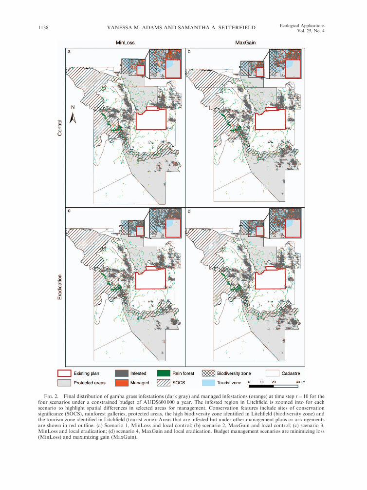
FIG. 2. Final distribution of gamba grass infestations (dark gray) and managed infestations (orange) at time step t¼ 10 for thefour scenarios under a constrained budget of AUD$600 000 a year. The infested region in Litchfield is zoomed into for eachscenario to highlight spatial differences in selected areas for management. Conservation features include sites of conservationsignificance (SOCS), rainforest galleries, protected areas, the high biodiversity zone identified in Litchfield (biodiversity zone) andthe tourism zone identified in Litchfield (tourist zone). Areas that are infested but under other management plans or arrangementsare shown in red outline. (a) Scenario 1, MinLoss and local control; (b) scenario 2, MaxGain and local control; (c) scenario 3,MinLoss and local eradication; (d) scenario 4, MaxGain and local eradication. Budget management scenarios are minimizing loss(MinLoss) and maximizing gain (MaxGain).


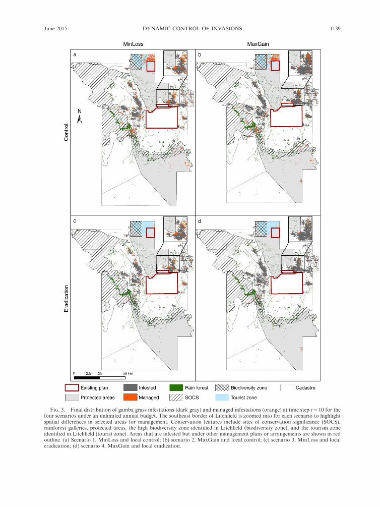
FIG. 3. Final distribution of gamba grass infestations (dark gray) and managed infestations (orange) at time step t¼ 10 for thefour scenarios under an unlimited annual budget. The southeast border of Litchfield is zoomed into for each scenario to highlightspatial differences in selected areas for management. Conservation features include sites of conservation significance (SOCS),rainforest galleries, protected areas, the high biodiversity zone identified in Litchfield (biodiversity zone), and the tourism zoneidentified in Litchfield (tourist zone). Areas that are infested but under other management plans or arrangements are shown in redoutline. (a) Scenario 1, MinLoss and local control; (b) scenario 2, MaxGain and local control; (c) scenario 3, MinLoss and localeradication; (d) scenario 4, MaxGain and local eradication.


looking to prevent the spread of the invasive species into

high value sites (Epanchin-Niell and Wilen 2012). The

relative performance of the MinLoss and MaxGain

strategies in our case study is consistent with previous

studies but is likely to reflect the rapid spread associated

with gamba grass and may not hold for other invasive

species with slower rates of spread. As such an

important next step will be to explore the generalizabil-

ity of our findings to a range of reasonable spread rates.

Given the rapid rate of spread in our study region,

under a limited budget it is best to control invasions

rather than invest in local eradication, which is

consistent with invasion management recommendations

(Panetta 2009). However, in our study region many of

the infested planning units are still at low density levels.

Therefore, it is more cost-effective to invest in eradica-

tion rather than control if there is an unlimited budget,

which is consistent with the nonspatial findings of

Adams and Setterfield (2013), which demonstrate that

for smaller infestations eradication is more cost effec-

tive. Given the rate of invasion, the size and density of

these infestations will rapidly increase such that if action

is delayed, eradication will no longer be a cost-effective

option and the costs of control will have dramatically

increased (over 10 year time frame there is an eightfold

increase in invasion given no management action). This

demonstrates the immediate need for strategic manage-

ment of gamba grass in the region in order to control the

infestations while management is still operationally

feasible and is consistent with recommendations to act

early in the invasion (Puth and Post 2005, Epanchin-

Niell and Wilen 2012).

Our study is the first study to our knowledge that

extends a static systematic conservation planning

approach (Januchowski-Hartley et al. 2011) to a multi-

year dynamic scheduling approach for strategic alloca-

tion of invasion management. By applying a systematic

conservation planning approach, we targeted planning

units that contributed to multiple targets (complemen-

tarity) thus delivering greater benefits than simply

targeting features based on cost effectiveness or simpli-

fied metrics of site value (e.g., Epanchin-Niell and Wilen

2012). In addition, by applying an existing and widely

used systematic conservation planning tool, Marxan, we

believe that our approach can be easily adapted to other

regions and species and may be more accessible to

managers. Furthermore, applying a multi-year approach

allowed us to estimate both the benefits of action in

terms of recovered and managed assets but also

prevented losses of assets from spread. It also provides

a more detailed understanding of how management

efforts will vary spatially and temporally by providing

annual allocations of efforts across planning units. For

example, if a static planning approach were taken, the

need to protect the southeast boundary of Litchfield

would not be identified as this only becomes a priority as

spread occurs from neighboring properties. In addition,

a multi-year scheduling approach allows for the

consideration of dynamic levels of management effort

and the associated costs. For example, the costs of

control are relatively stable through time while eradica-

tion costs are much larger in the first years of the

program and then dramatically decline through time. By

allocating effort through time, the variable levels of

funding through a control or eradication program can

be estimated and planned for to ensure that adequate

resources are available for the duration of treatment.

An important aspect of dynamic planning is the effect

of uncertainty on decision making and outcomes.

Visconti et al. (2010a) found that depending on

uncertainty levels, using a MaxGain approach can

deliver better results. Given our limited understanding

of rates and patterns of spread of gamba grass, our

estimated spread rate and distance for use in our

simulations have high levels of associated uncertainty.

A necessary next step would be to quantify the levels of

uncertainty associated with the spread model and

incorporate this into the decision framework to assess

the robustness of strategies to this uncertainty.

Our results are consistent with the generalized spatial-

dynamic problems explored by Epanchin-Niell and

Wilen (2012), in particular that the optimal strategy

(control or eradicate) depends both on the available

resources and the level and location of invasion relative

to the overall landscape. However, our approach also

provides insights into the utility of applying systematic

conservation planning principles. For example, we

prioritized infestations with multiple conservation fea-

tures, such as the boundary of the invasion in Litchfield

where the biodiversity and tourism zones overlap,

demonstrating a central tenet of systematic conservation

planning: complementarity (i.e., conservation areas

should be selected to maximize the differences in their

biotic content [Sarkar et al. 2006]). Our approach

provides insights into both the utility of spatial-dynamic

planning and systematic conservation planning in

prioritizing management of invasive species.

ACKNOWLEDGMENTS

This work was funded by a RIRDC National Weeds andProductivity Program research grant (PRJ-006928).

LITERATURE CITED

Adams, V. M., and S. A. Setterfield. 2012. Spatial prioritisationfor management of gamba grass (Andropogon gayanus)invasions: accounting for social, economic and environmen-tal values. Pages 49–52 in 18th Australasian Weeds Confer-ence. Weed Society of Victoria, Melbourne, Victoria,Australia.

Adams, V. M., and S. A. Setterfield. 2013. Estimating thefinancial risks of Andropogon gayanus to greenhouse gasabatement projects in northern Australia. EnvironmentalResearch Letters 8:025018.

Ball, I. R., M. E. Watts, and H. P. Possingham. 2009. Marxanand relatives: Software for spatial conservation prioritisation.Pages 185–195 in A. Moilanen, K. A. Wilson, and H. P.Possingham, editors. Spatial conservation prioritization:quantitative methods and computational tools. OxfordUniversity Press, New York, New York, USA.


Brooks, K. J., S. A. Setterfield, and M. M. Douglas. 2010.Exotic grass invasions: applying a conceptual framework tothe dynamics of degradation and restoration in Australia’stropical savannas. Restoration Ecology 18:188–197.

Brooks, M. L., C. M. D’Antonio, D. M. Richardson, J. B.Grace, J. E. Keeley, J. M. Ditomaso, R. J. Hobbs, M.Pellant, and D. Pyke. 2004. Effects of invasive alien plants onfire regimes. BioScience 54:677–688.

Buckley, Y. M., E. Brockerhoff, L. Langer, N. Ledgard, H.North, and M. Rees. 2005. Slowing down a pine invasiondespite uncertainty in demography and dispersal. Journal ofApplied Ecology 42:1020–1030.

Butchart, S. H. M., et al. 2010. Global biodiversity: indicatorsof recent declines. Science 328:1164–1168.

DEH. 2004. Managing invasive species in Australia: successstories—biological control of Mimosa. Department ofEnvironment and Heritage (DEH), Canberra, Australia.

DLRM. 2014. Weed management plan for Andropogan gayanus(Gamba grass). Northern Territory Government Departmentof Land Resource Management (DLRM), Palmerston,Australia.

Ehrenfeld, J. G. 2010. Ecosystem consequences of biologicalinvasions. Annual Review of Ecology, Evolution, andSystematics 41:59–80.

Epanchin-Niell, R. S., and A. Hastings. 2010. Controllingestablished invaders: integrating economics and spreaddynamics to determine optimal management. Ecology Letters13:528–541.

Epanchin-Niell, R. S., and J. E. Wilen. 2012. Optimal spatialcontrol of biological invasions. Journal of EnvironmentalEconomics and Management 63:260–270.

Hutley, L. B., and S. A. Setterfield. 2008. Savannas. Pages3143–3154 in S. E. Jørgensen and B. Fath, editors.Encyclopedia of ecology. Elsevier, Amsterdam, The Nether-lands.

Januchowski-Hartley, S., P. Visconti, and R. Pressey. 2011. Asystematic approach for prioritizing multiple managementactions for invasive species. Biological Invasions 13:1241–1253.

Kingsford, R. T., et al. 2009. Major conservation policy issuesfor biodiversity in Oceania. Conservation Biology 23:834–840.

Northern Territory Government. 2009. Weed risk assessmentreport: Andropogon gayanus (gamba grass). Northern Terri-tory Government, Palmerston, Australia.

NRETAS. 2009. Recognising sites of conservation significancefor biodiversity values in the Northern Territory. BiodiversityConservation Unit, Department of Natural Resources,Environment, The Arts and Sport, Palmerston, Australia.

Panetta, F. D. 2007. Evaluation of weed eradication programs:containment and extirpation. Diversity and Distributions13:33–41.

Panetta, F. D. 2009. Weed eradication—an economic perspec-tive. Invasive Plant Science and Management 2:360–368.

Panetta, F. D., S. Csurhes, A. Markula, and M. Hannan-Jones.2011. Predicting the cost of eradication for 41 class 1 declaredweeds in Queensland. Plant Protection Quarterly 26:42–46.

Petty, A. M., S. A. Setterfield, K. B. Ferdinands, and P.Barrow. 2012. Inferring habitat suitability and spreadpatterns from large-scale distributions of an exotic invasive

pasture grass in north Australia. Journal of Applied Ecology49:742–752.

Pimentel, D., R. Zuniga, and D. Morrison. 2005. Update on theenvironmental and economic costs associated with alien-invasive species in the United States. Ecological Economics52:273–288.

Possingham, H. P., A. Moilanen, and K. A. Wilson. 2009.Accounting for habitat dynamics in conservation planning.Pages 135–144 in A. Moilanen, K. A. Wilson, and H. P.Possingham, editors. Spatial conservation prioritization:quantitative methods and computational tools. OxfordUniversity Press, New York, New York, USA.

Pressey, R. L., M. E. Watts, and T. W. Barrett. 2004. Ismaximizing protection the same as minimizing loss? Efficien-cy and retention as alternative measures of the effectivenessof proposed reserves. Ecology Letters 7:1035–1046.

Puth, L. M., and D. M. Post. 2005. Studying invasion: have wemissed the boat? Ecology Letters 8:715–721.

Rossiter, N. A., S. A. Setterfield, M. M. Douglas, and L. B.Hutley. 2003. Testing the grass-fire cycle: alien grass invasionin the tropical savannas of northern Australia. Diversity andDistributions 9:169–176.

Sarkar, S., et al. 2006. Biodiversity conservation planning tools:present status and challenges for the future. Annual Reviewof Environment and Resources 31:123–159.

Setterfield, S. A., N. A. Rossiter-Rachor, M. M. Douglas, D.McMaster, V. M. Adams, and K. Ferdinands. 2014. Theimpacts of Andropogon gayanus (gamba grass) invasion onthe fire danger index and fire management at a landscapescale. Pages 125–128 in 19th Australasian Weeds Conference.Weed Society of Tasmania, Hobart, Tasmania, Australia.

Setterfield, S. A., N. A. Rossiter-Rachor, L. B. Hutley, M. M.Douglas, and R. J. Williams. 2010. Turning up the heat: theimpacts of Andropogon gayanus (gamba grass) invasion onfire behaviour in northern Australian savannas. Diversity andDistributions 16:854–861.

Simberloff, D. 2009. We can eliminate invasions or live withthem. Successful management projects. Biological Invasions11:149–157.

Steel, J., J. Weiss, and T. Morfe. 2014. Using a temporal-spatialeconomic model of serrated tussock spread to illustrate theoutcomes of different control strategies. State of VictoriaDepartment of Environment and Primary Industries, Mel-bourne, Australia.

Stewart, R. R., and H. P. Possingham. 2005. Efficiency, costsand trade-offs in marine reserve system design. Environmen-tal Modeling and Assessment 10:203–213.

Visconti, P., R. L. Pressey, M. Bode, and D. B. Segan. 2010a.Habitat vulnerability in conservation planning—when itmatters and how much. Conservation Letters 3:404–414.

Visconti, P., R. L. Pressey, D. B. Segan, and B. A. Wintle.2010b. Conservation planning with dynamic threats: the roleof spatial design and priority setting for species’ persistence.Biological Conservation 143:756–767.

Williams, N. S. G., A. K. Hahs, and J. W. Morgan. 2008. Adispersal-constrained habitat suitability model for predictinginvasion of alpine vegetation. Ecological Applications18:347–359.

Wilson, K. A., M. F. McBride, M. Bode, and H. P.Possingham. 2006. Prioritizing global conservation efforts.Nature 440:337–340.

SUPPLEMENTAL MATERIAL

Ecological Archives

The Appendix is available online: http://dx.doi.org/10.1890/14-1062.1.sm


http://dx.doi.org/10.1890/14-1062.1.sm

Documents

Optimal dynamic control of invasions: applying a